Let me start with a small library.

It has a long shelf of books. Every month, a clerk brings in a new delivery and puts the books on the shelf, one stack at a time. It takes him a few minutes.

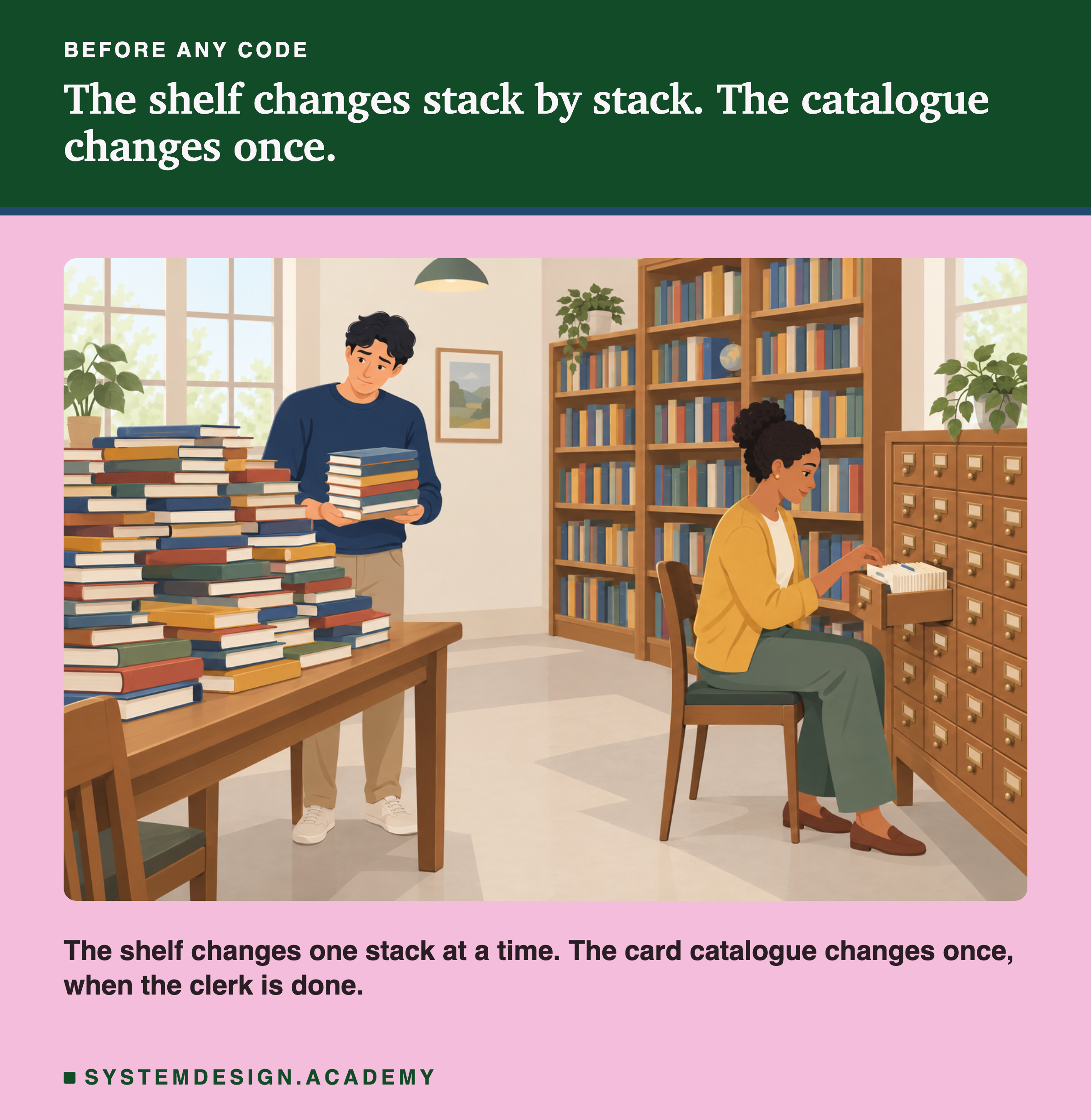
Now a visitor walks in during those few minutes. She wants to count how many books the library holds. She counts what is on the shelf. Her number is wrong. It is not last month's number, and it is not this month's number either. It is something in between, because the clerk is only part way through.

There is a second way to count. Next to the shelf there is a card catalogue. The clerk writes the new cards only when every stack is on the shelf. If the visitor counts the cards instead of the shelf, she gets last month's number before the clerk is done, and this month's number after. Never anything in between.

In this lesson, the shelf is a folder of data files. The card catalogue is a small log that lists which files belong to the table. A system built around such a log is called a lakehouse. I will show you, with real numbers, what goes wrong when you count the shelf.

This is the first lesson of a new chapter on data engineering for large systems: lakehouses, Spark, and fast analytics databases. Other lessons on this site already cover some of the ground, and I will not repeat them.

The lesson on data lakes explains schema-on-read, deciding what data means only when reading it. It also explains the bronze, silver and gold layers: raw, cleaned and ready-to-use copies. The lesson on data warehousing explains star schemas, a fact table ringed by lookup tables. ETL and ELT, two orders for copying and cleaning data, each have their own lesson. So does the data catalog, a searchable list of a company's tables. In the AI course, Data Lakes, Warehouses, and Lakehouses for ML measures four other lakehouse problems. They are a bad value in a file, a backfill, many tiny files, and old files deleted too soon.

This lesson asks one question, and measures it. What is a lakehouse, and what breaks if a "table" is just a folder of Parquet files? The answer I measured is about one thing: what a reader sees while a writer is in the middle of a change.

I explain every word first, in plain English, starting with the oldest of the three ideas: the warehouse. What problem was it built to solve?

Think about a shop. Its main database handles one sale at a time: a customer pays, one row is written. That database is fast for small, single changes. But the manager asks a different kind of question. "What were total sales per city, per month, for the last three years?" That question reads millions of old rows at once, and it slows down the database that takes the payments.

So companies built a second database just for those big questions. Every night, they copy the day's data into it. It keeps years of history. It is tuned to read huge numbers of rows quickly, not to write one row quickly. That second database is called a data warehouse, a database built for questions over history.

A warehouse is strict. Before data goes in, you must say exactly what columns it has and what type each column is. Data that does not fit is refused at the door. It also stores the data in its own private format, inside the product. To read it, you go through the warehouse's own engine.

The CIDR 2021 paper that defined the lakehouse gives Amazon Redshift and Snowflake as examples of warehouses. The strictness is a real strength: the numbers are clean and the queries are fast. But it has a cost. Storage inside a warehouse is not cheap, and some data does not fit a strict table at all: images, logs, audio, raw text.

So where did the data that did not fit go?

It went into plain files, in cheap storage. A company takes everything it has, as files, and puts it in one big storage service that charges very little per gigabyte, like Amazon S3. Any program can read the files later. Nobody checks the columns on the way in. You decide what the data means when you read it. That pile of files is called a data lake, cheap storage holding files in open formats.

For tables, a common file format in a lake is Parquet. A Parquet file stores one piece of a table, column by column, with a short description at the end. The CIDR paper describes lakes in these words: "low-cost storage systems with a file API that hold data in generic and usually open file formats". It names Parquet as one of them.

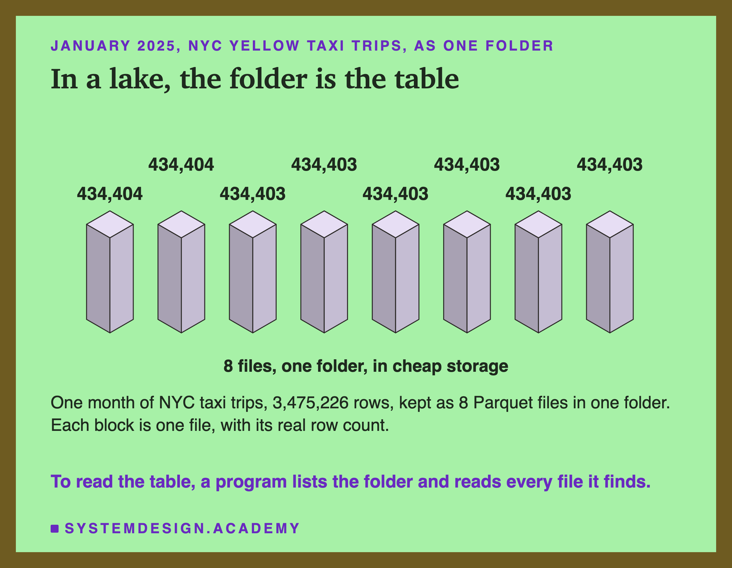
The figure shows the data this lesson uses. It is one month of real New York taxi trips, January 2025, from the city's Taxi and Limousine Commission. The month has 3,475,226 trips. I cut it into 8 Parquet files, and each file holds about one eighth. 3,475,226 divided by 8 is 434,403.25, so two files hold 434,404 rows and six hold 434,403.

In a lake, a table is often nothing more than this: a folder of Parquet files. To read the table, a program lists the folder and reads every file it finds. Keep that sentence in mind. The whole lesson is about it.

For years, many companies ran a lake and a warehouse side by side. The raw data went into the lake first, because it was cheap. Then a second job copied the cleaned part into the warehouse, because the warehouse was fast and strict. That meant two storage systems for one company's data.

The copying jobs have names. ETL means extract, transform, load: take data out, clean it, then load it in. ELT does the same steps in a different order: load first, then clean inside the warehouse. The paper puts the cost plainly: "data is first ETLed into lakes, and then again ELTed into warehouses, creating complexity, delays, and new failure modes." It also says this setup, a lake plus a warehouse, was, in the authors' experience, "used at virtually all Fortune 500 enterprises".

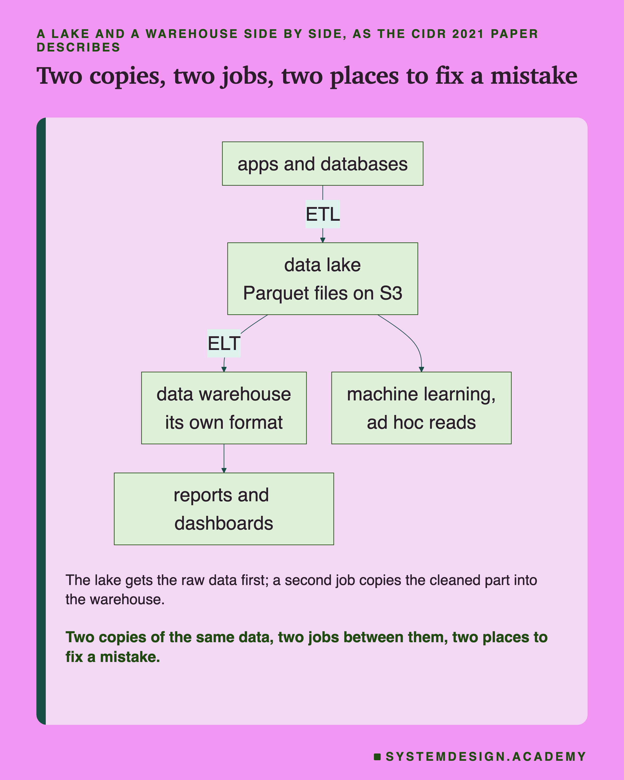
The flowchart shows the whole path. Raw data goes into the lake through ETL, and a second job, ELT, copies the cleaned part into the warehouse. Reports read the warehouse; machine learning and one-off questions often read the lake.

So a company paid twice. It stored the data twice. It ran jobs between the two copies. When a number was wrong, someone had to find out which copy was wrong, and why. And the newest data was often only in the lake, because the warehouse copy often ran only once a night.

The obvious question follows. Could one system give the cheap open files of a lake and the strict, safe tables of a warehouse at the same time?

The answer the paper gives is the lakehouse. Here is its definition, word for word. A lakehouse is "a data management system based on low-cost and directly-accessible storage that also provides traditional analytical DBMS management and performance features such as ACID transactions, data versioning, auditing, indexing, caching, and query optimization."

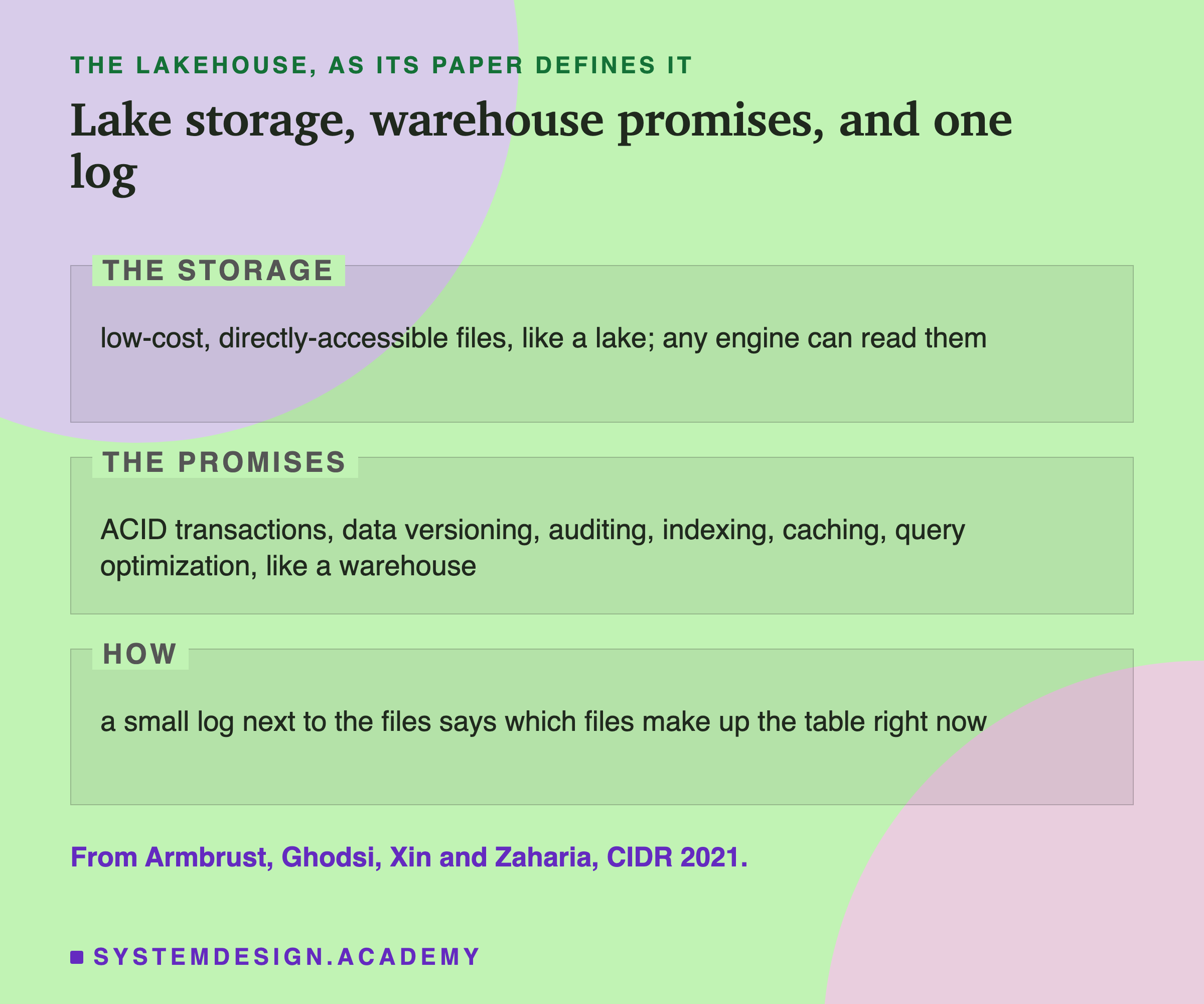
Let me take that sentence apart. "Low-cost and directly-accessible storage" means the lake's cheap files, which any program can open. The letters DBMS just stand for database management system. The rest is a list of things a warehouse promises.

The first promise on the list is the one this lesson tests. ACID is a set of four guarantees a database makes about each change, explained in the ACID properties lesson. Here I need only the first. A is for atomic: a change happens completely, or not at all. A reader never sees half of it.

So a lakehouse is a lake whose files get warehouse-style promises. A lakehouse table keeps its data in ordinary Parquet files. Something extra sits next to those files to make the promises true.

What is that extra thing, and how small can it be?

The extra thing is a list. Next to the data files, the table keeps a small folder of notes. Each note says which files were added to the table and which were taken away. Read in order, the notes give the full list of files that make up the table right now. A reader never lists the data folder. It reads the notes, and then opens only the files they name. That folder of notes is called a transaction log, the table's own list of which files count.

A writer works in two steps. First it writes its new data files. Nobody reads them yet, because no note names them. Then it adds one new note that names them. Adding that one note is called a commit, the single moment a change becomes real.

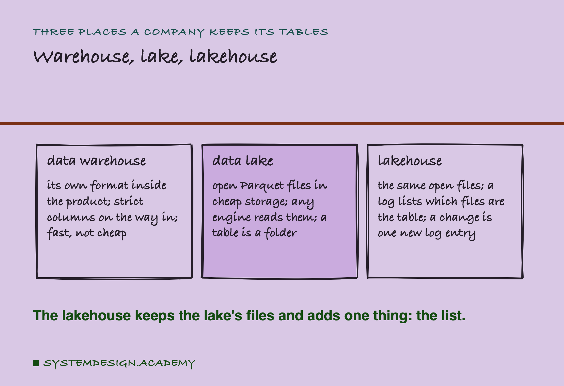
The three cards put the three ideas side by side. The warehouse keeps its own format and checks everything at the door. The lake keeps open files and checks nothing. The lakehouse keeps the lake's open files, and adds the list.

This idea has several written versions. The best known is Delta Lake. Its rule book, which every Delta tool must follow, describes the same two steps. Writers "optimistically write out new data files". Then "they commit, creating the latest atomic version of the table by adding a new entry to the log." It also says readers "only see one consistent snapshot of a table at time by using the transaction log to selectively choose which data files to process."

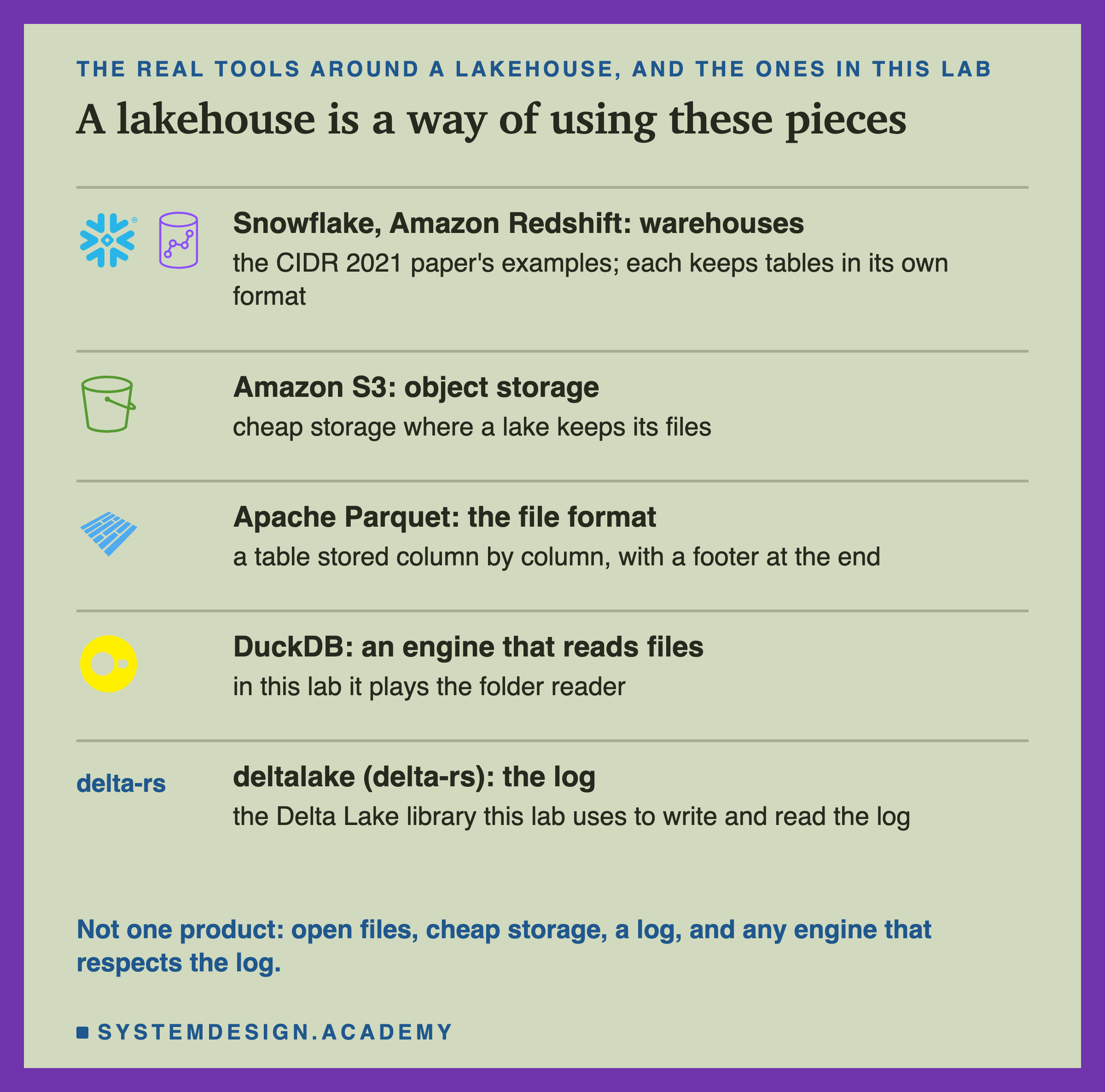
These are the real tools around a lakehouse, and the ones in my lab. A lakehouse is not one product you buy. It is the open files, in cheap storage, plus a log, plus any engine that respects the log. Delta Lake, Apache Iceberg and Apache Hudi are three formats for that log, and lesson 2 of this chapter opens each one up.

A Parquet file starts with four bytes, the letters PAR1. Then come the data, cut into blocks of rows. Each block stores its rows column by column. A block like that is called a row group, a slice of rows stored column by column.

At the very end of the file sits a short description. It says where each column of each row group starts, how many rows there are, and what type each column has. That description is called the footer, the file's table of contents at the end. After the footer come its length and PAR1 again. The Parquet documentation lays the file out in exactly that order.

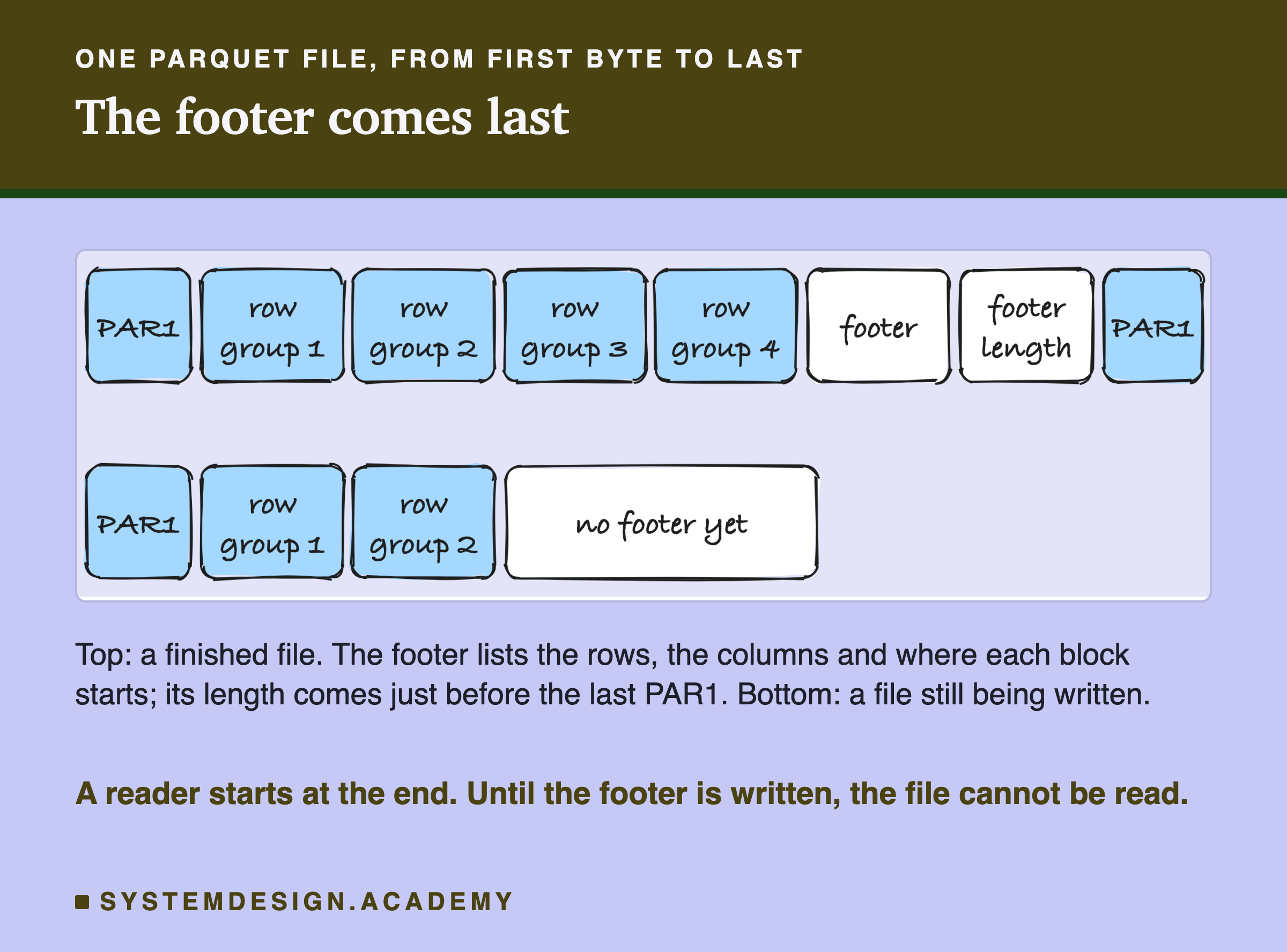
A reader starts at the end. It reads the last bytes, finds the footer, and only then knows where everything is. This is why counting rows in a Parquet file is fast: the count is in the footer, so a reader does not touch the data at all.

It also means something less pleasant. A Parquet file that is still being written has no footer yet. To a reader, it is not a smaller table. It is a broken file. The real January file from the city, for example, has 4 row groups and one footer for its 3,475,226 rows; the report script counts both.

So far: a warehouse is strict and fast, with its own format. A lake is cheap open files, where a table is a folder. A lakehouse adds a log that lists which files are the table, and a change becomes real in one commit. Now I want to test what that log actually buys you. How do I set that test up?

The test needs two programs. A writer adds data to a table. A reader counts the rows in the table. The question is simple: what does the reader see while the writer is in the middle of its work?

I used two real months of the NYC taxi data. January 2025 is the table that already exists: 3,475,226 trips. February 2025 is the new data the writer adds: 3,577,543 trips. When the writer is done, the table must hold 3,475,226 + 3,577,543 = 7,052,769 trips. Those two numbers, before and after, are the only correct answers a reader should ever get.

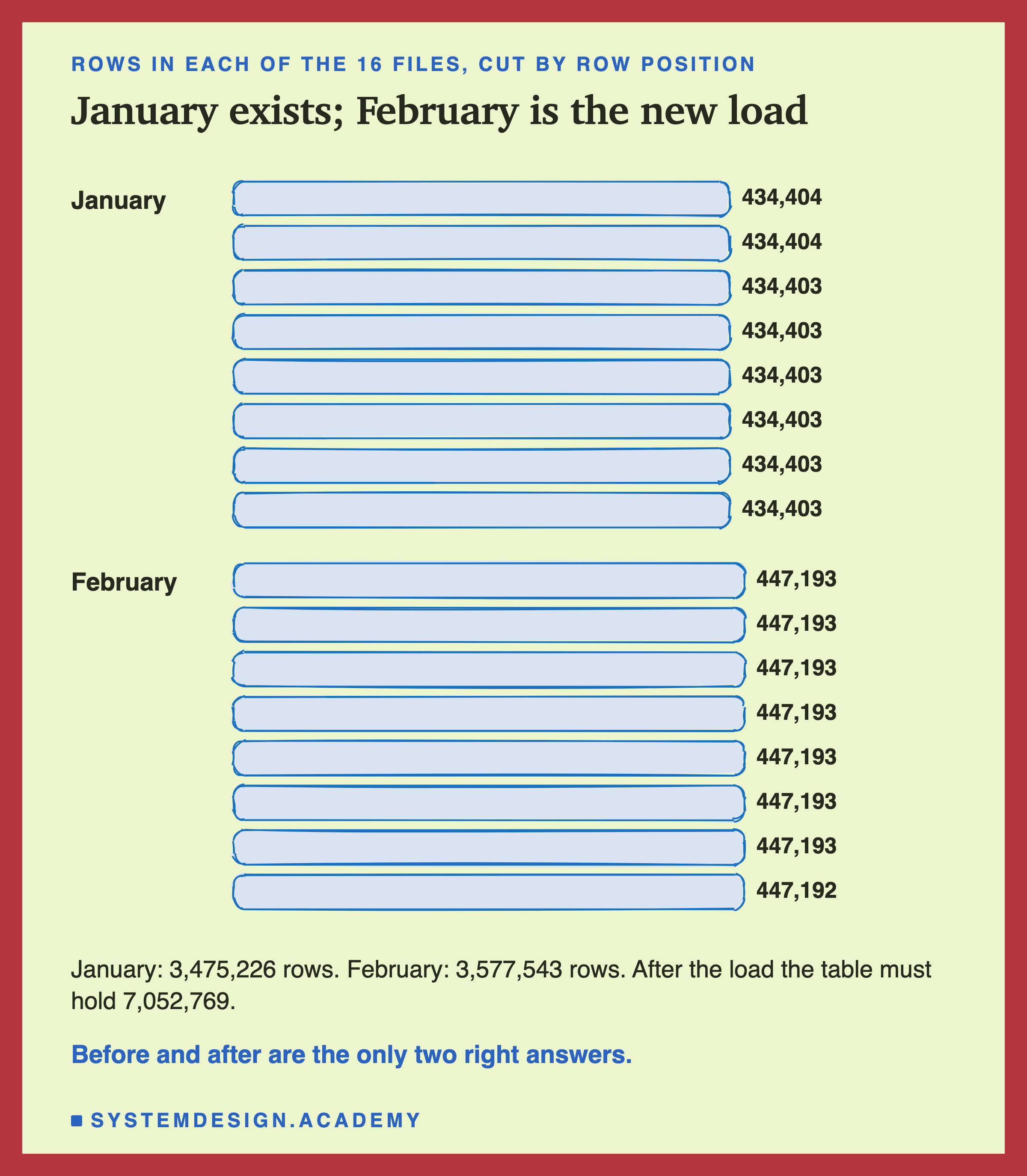
Each month is 8 files, cut by row position into nearly equal parts. February's 3,577,543 rows over 8 files gives 447,192.875, so seven files hold 447,193 rows and one holds 447,192. Writing a month as several files is normal. Big systems write many files at once so that many machines can work in parallel.

I built the table twice from the same files. The plain table is a folder of Parquet files. Its reader lists the folder and counts every row in every file it found. In the step test, it counts with DuckDB, a small database engine that reads Parquet files directly. In the race, it reads each listed file's footer with pyarrow's read_metadata and adds up the row counts written there. The Delta table is the same files plus a Delta Lake log. I built it with deltalake, the Python package of the delta-rs project. Its reader opens the log and counts only the files the log names.

I ran the test in two ways. First, step by step: the writer adds one file, stops, and the reader looks. That shows every possible moment, one by one. Second, as a real race, with nothing paused. What does the step-by-step version show for the plain folder?

Here is the plain folder. At the start, it holds January's 8 files, and the reader counts 3,475,226 rows. Correct. Then the writer adds February's first file, and the reader looks again.

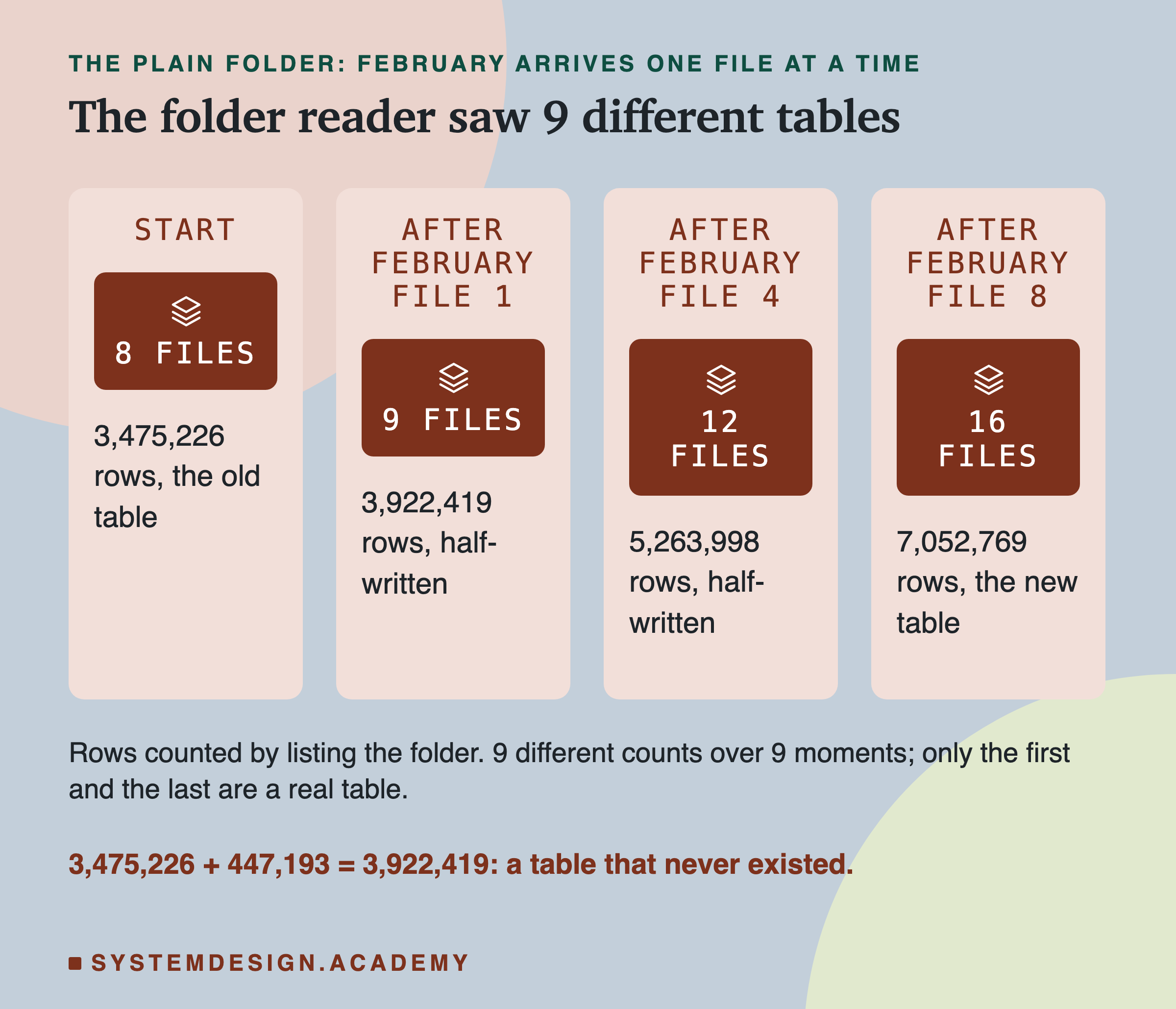
After one file, the folder holds 9 files, and the reader counts 3,475,226 + 447,193 = 3,922,419 rows. That number is not January, and it is not January plus February. No such table ever existed. After four files, it counts 5,263,998. Only after the eighth file does it reach the right answer, 7,052,769.

So the reader saw 9 different row counts: the old one, the new one, and 7 in between. I will call each of the 7 middle ones a half-written table, a table state that was never meant to exist.

Row counts may look harmless, so let me show what they do to a real answer. Suppose the reader is a dashboard that adds up the money taken, the total_amount column. January alone took $89,005,026.80. After February's first file, the dashboard shows $89,005,026.80 + $11,466,024.76 = $100,471,051.56. February's total is not in there, and neither is January's on its own. Someone in a meeting might read it as "January and early February". It is neither. It is whatever the clerk had shelved.

The folder has no way to say "wait, I am not done". The reader has no way to ask. Does the Delta table do any better with the very same files?

I ran the same steps on the Delta table. The writer wrote the same 8 February files into the table folder, one at a time. After each file, I asked two questions: what does a folder listing see, and what does a Delta reader see? Only after all 8 files existed did the writer add its one log entry.

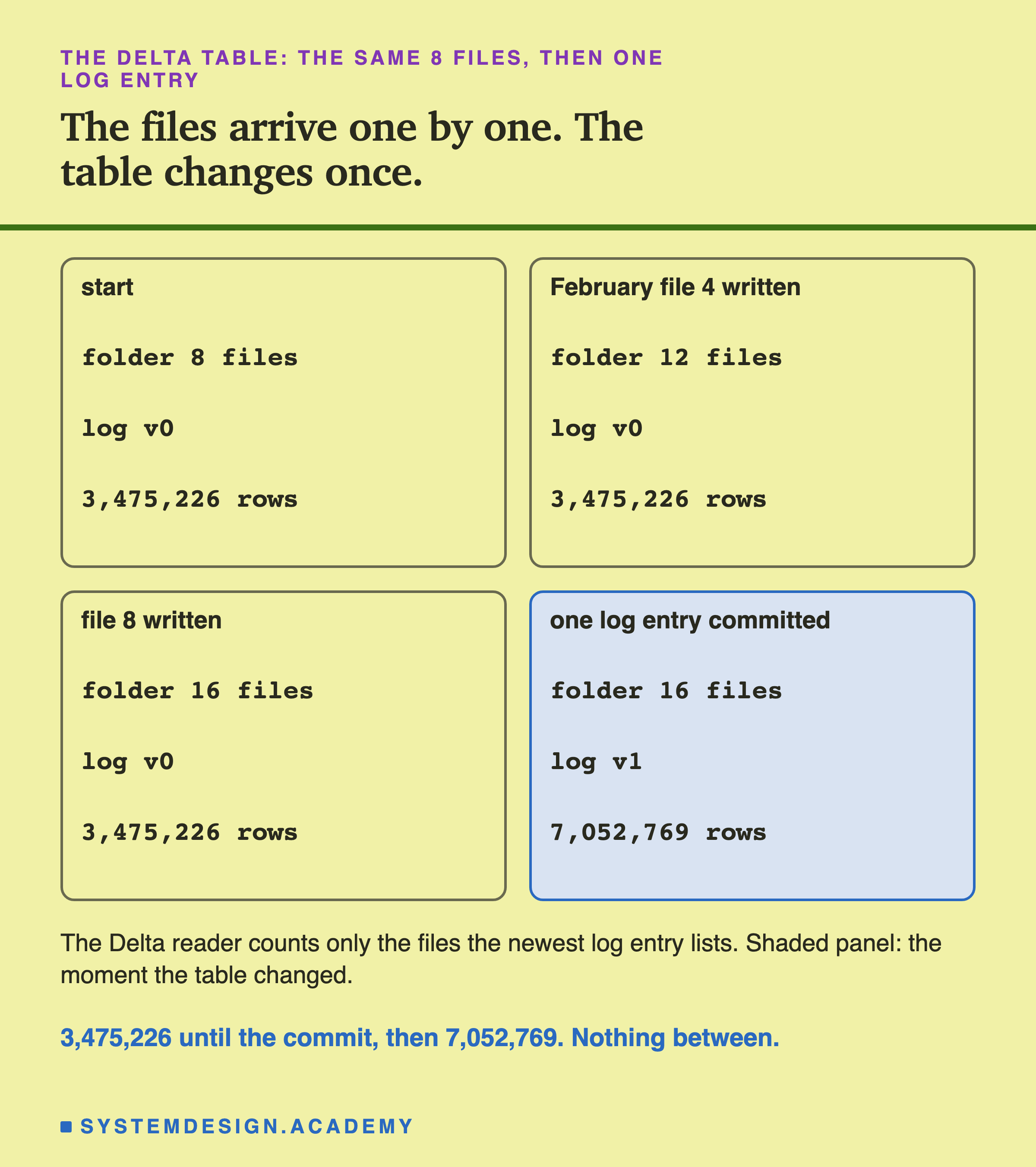
The folder listing behaved exactly like before: 9 files, then 10, then up to 16. The new files were really there, on disk, in the table's own folder. But the Delta reader did not count them. It counted 3,475,226 rows after every one of the 8 files, because the log still said "version 0, these 8 January files". Then the writer added one log file, and the next read counted 7,052,769.

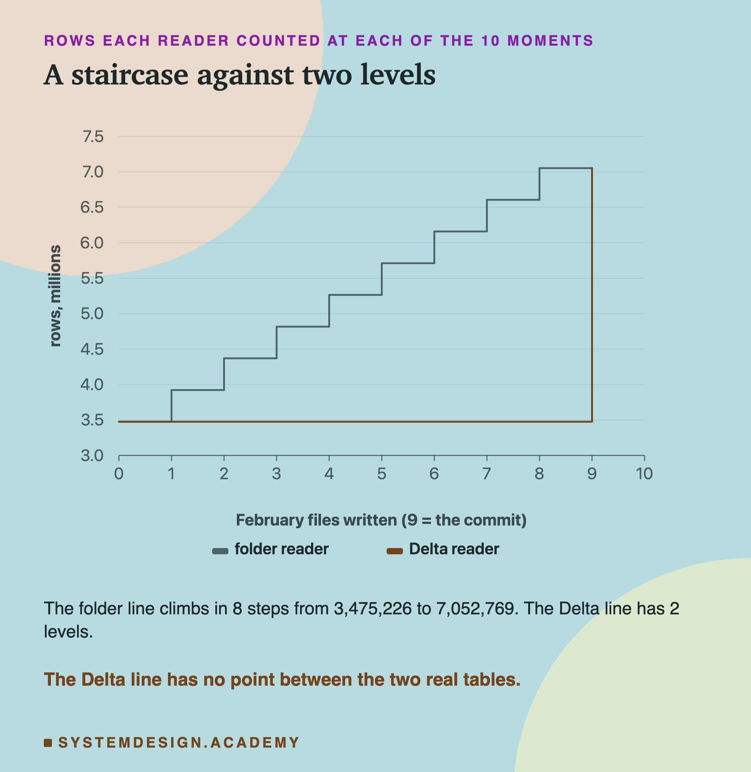
The chart puts the two readers on one axis. The folder reader climbs a staircase of 8 steps. The Delta reader has only two levels. Each level is a whole table that really existed: version 0 and version 1. A numbered state of the table like that is called a version, one complete state of the table.

A Delta version, then, is the card catalogue from the first slide. The 8 Parquet files are the stacks of books on the shelf. The visitor who reads the catalogue never counts a half-filled shelf. But what is actually inside that one log entry, and why is writing it a single step?

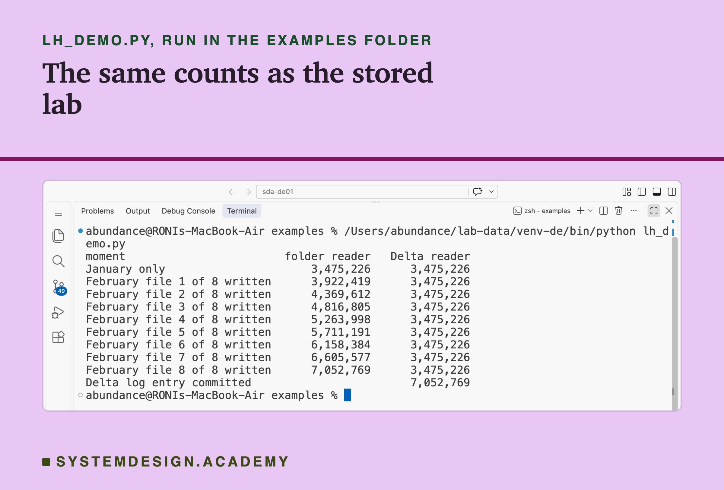
To show a real log, I ran a short script, lh_log_peek.py. It writes January with the normal deltalake call, write_deltalake, appends February with a second call, and then prints what is in the log. Here is that run, recorded in a real terminal.

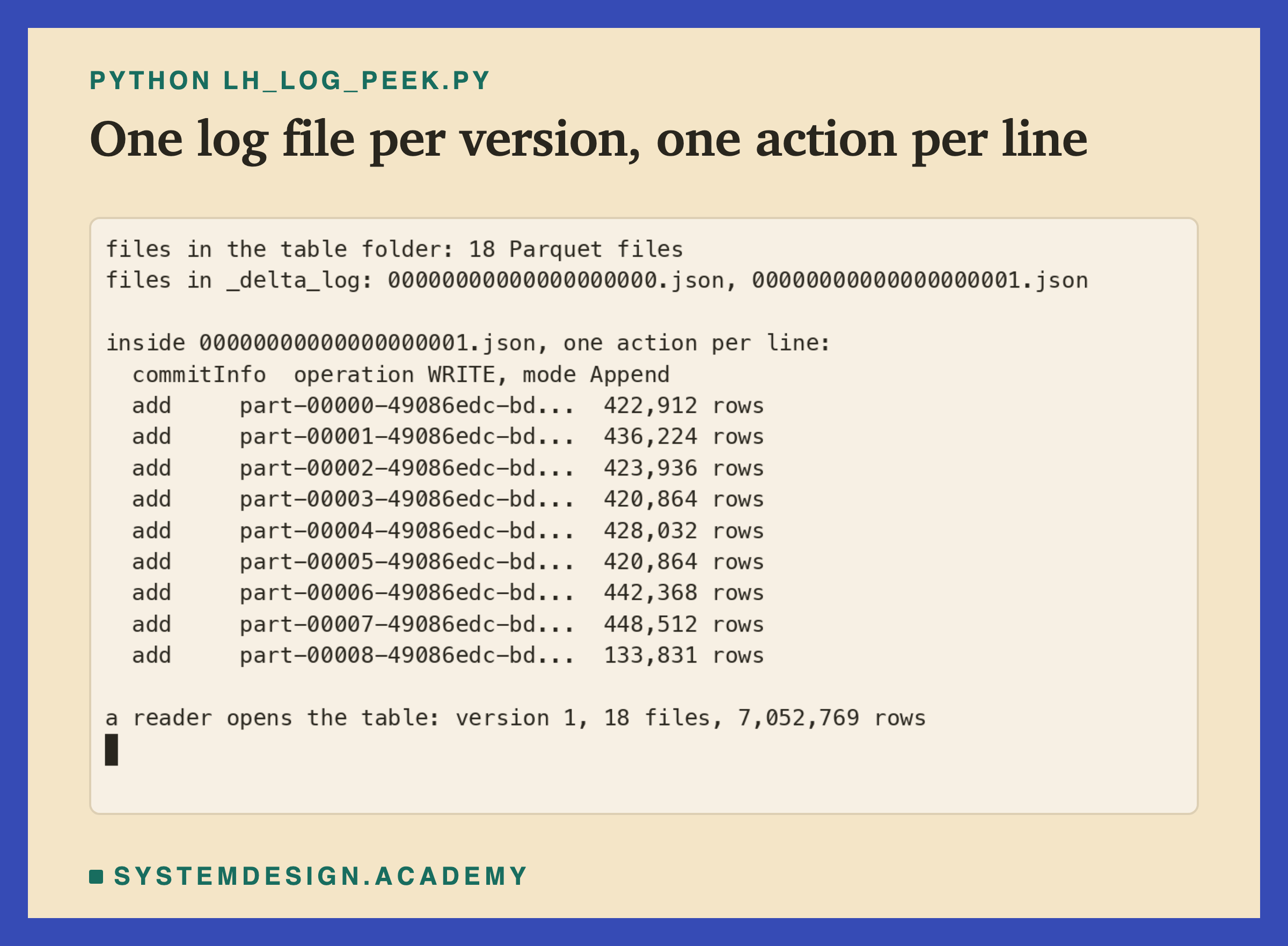
The log folder is called _delta_log. It holds one JSON file per version, named with the version number padded to 20 digits: 00000000000000000000.json is version 0, and 00000000000000000001.json is version 1. Each file is JSON, a plain text format for structured data.

Each line inside the file is one instruction. A line like that is called an action, one change in the list. An add action names a data file that is now part of the table, with its size and, usually, its row count. A remove action names a file that is no longer part of it.

Here deltalake chose its own split, 9 files for each month, so version 1 holds 9 add lines. There is also one commitInfo line, which records when, how, and with which program the entry was written. When the row counts are there, a reader can know the table size before it opens any data.

The sequence below follows one append from the writer's side and the reader's side at the same time.

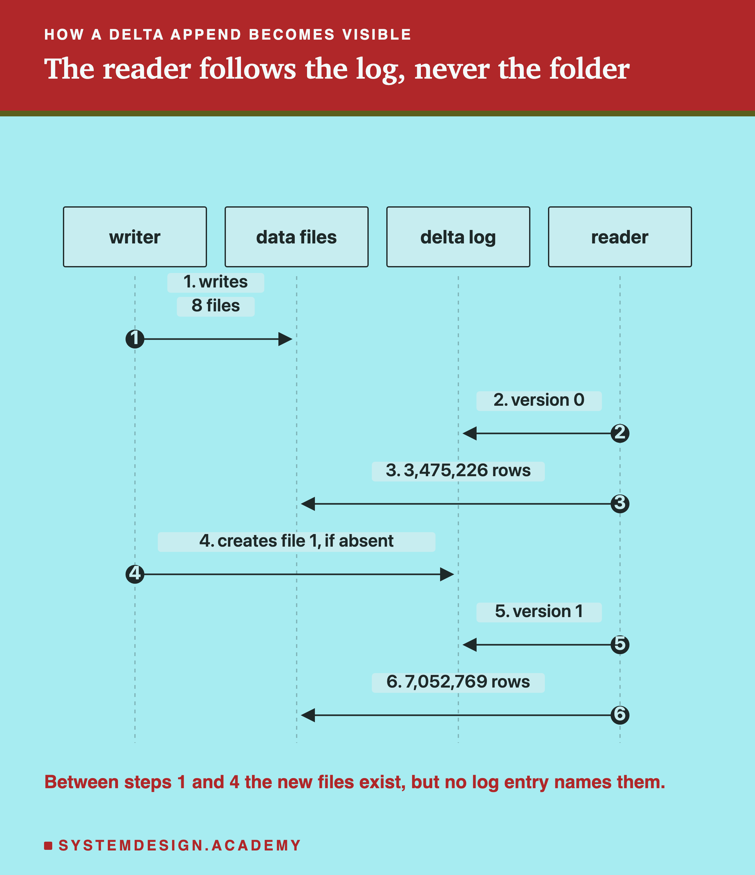
Why is a commit a single step? Because it is one new file, and one file appears at once. The Delta rule book calls these files "the unit of atomicity for a table". A writer must create version file number 1 only if no file with that name exists yet. That rule, create a file only if nobody else has, is called put-if-absent. If two writers both try to create file number 1, only one succeeds; the other learns it lost and must try again. Lesson 3 of this chapter measures exactly that fight.

So far I have only added data. Real tables also replace data. What happens when a writer needs to fix a month?

Here is a common job. January's data has a problem, and the team wants to replace it with a corrected copy. In the real January file, 144,118 trips have a fare below zero. My corrected January simply drops them: 3,475,226 − 144,118 = 3,331,108 trips. Replacing a table's old data with new data is called an overwrite.

On a plain folder, a careful writer writes the 8 corrected files first, and only then deletes the 8 old ones. That way the folder is never empty. I ran exactly that, one step at a time, and let the reader look after each of the 16 steps.

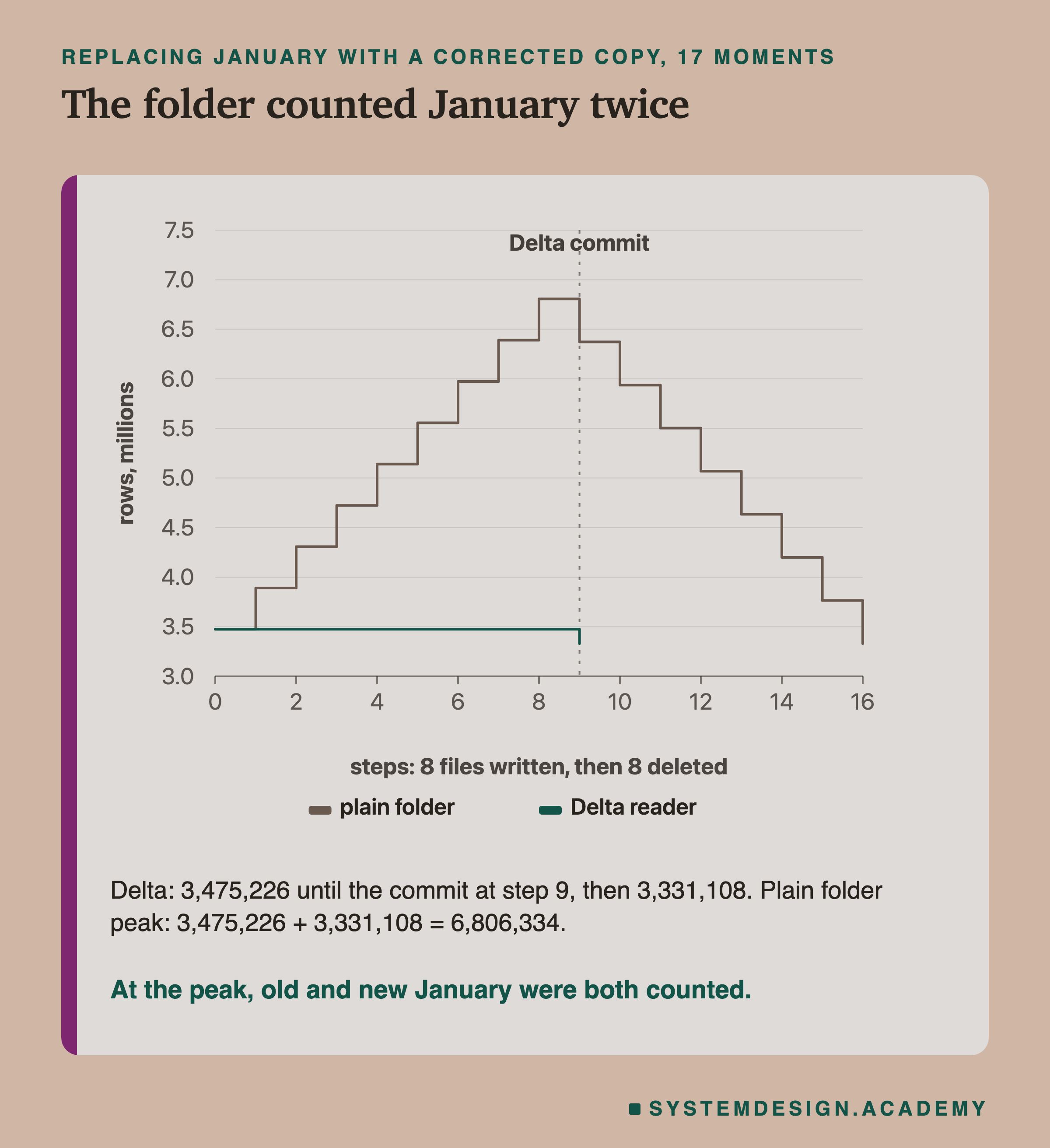
At the peak, the folder held the old and the new January together, and the reader counted 3,475,226 + 3,331,108 = 6,806,334 trips for one month. The money looked even worse. The dashboard would have shown $179,340,134.65 for January, about twice the corrected total of $90,335,107.85. Deleting the old files first and writing the new ones second would only flip the problem: the folder would be half empty instead of double full.

On the Delta table, the writer wrote the same 8 corrected files, then committed one log entry that holds 8 remove actions and 8 add actions together. The reader counted 3,475,226 until the commit, and 3,331,108 after it. Nothing between.

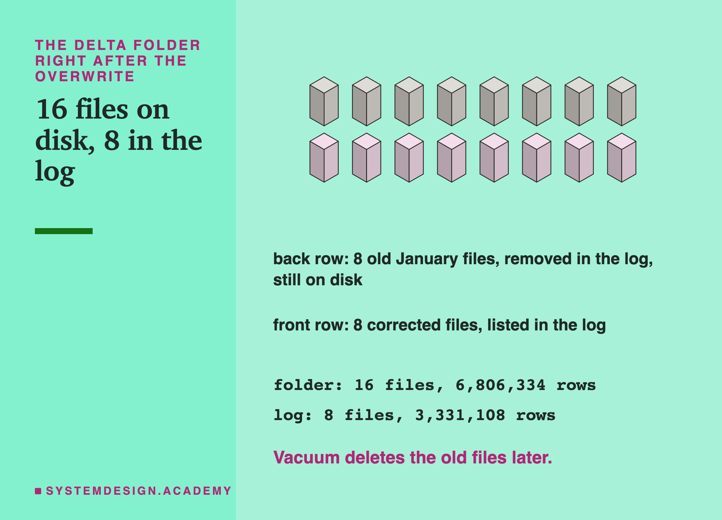
There is a catch, and it surprises people. After the commit, the old January files are still on disk. The log says they are removed, but nobody deleted them. Suppose a program lists the Delta table's folder instead of reading its log. It counts all 16 files and 6,806,334 rows, the same wrong number as the plain folder at its worst.

Two programs that run at the same time and touch the same data are in a race, where the result depends on timing. In the race test, a reader process counted rows over and over, as fast as it could. For the plain folder it read each listed file's footer; for the Delta table it opened the log. At the same time, a writer process did its job with the normal library calls.

For the plain folder, the writer saved each file with pyarrow. For the Delta table, it called write_deltalake once, which writes the files and then the log entry by itself. A race comes out a little differently every time, so I ran each of the four cases 5 times.

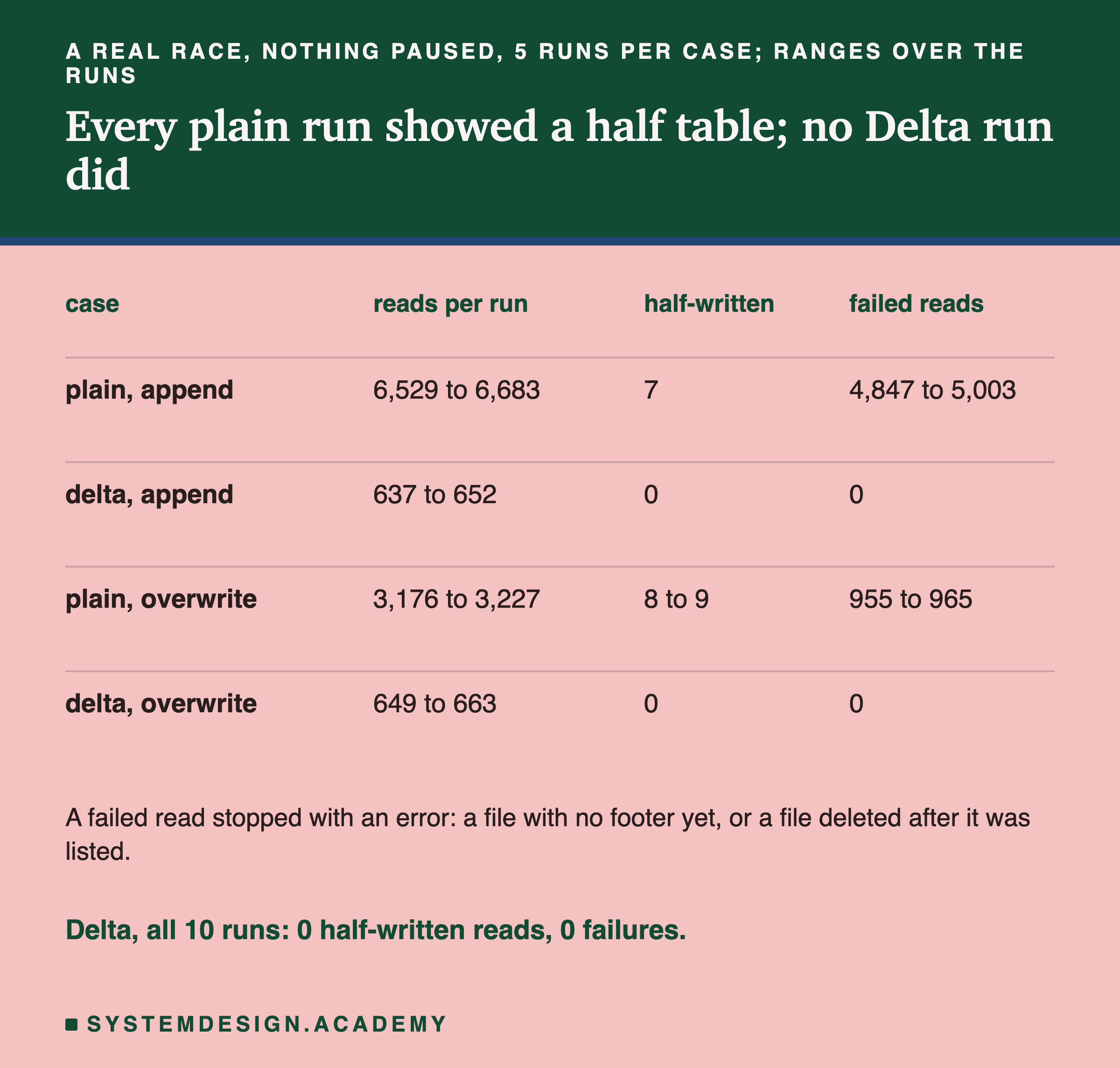
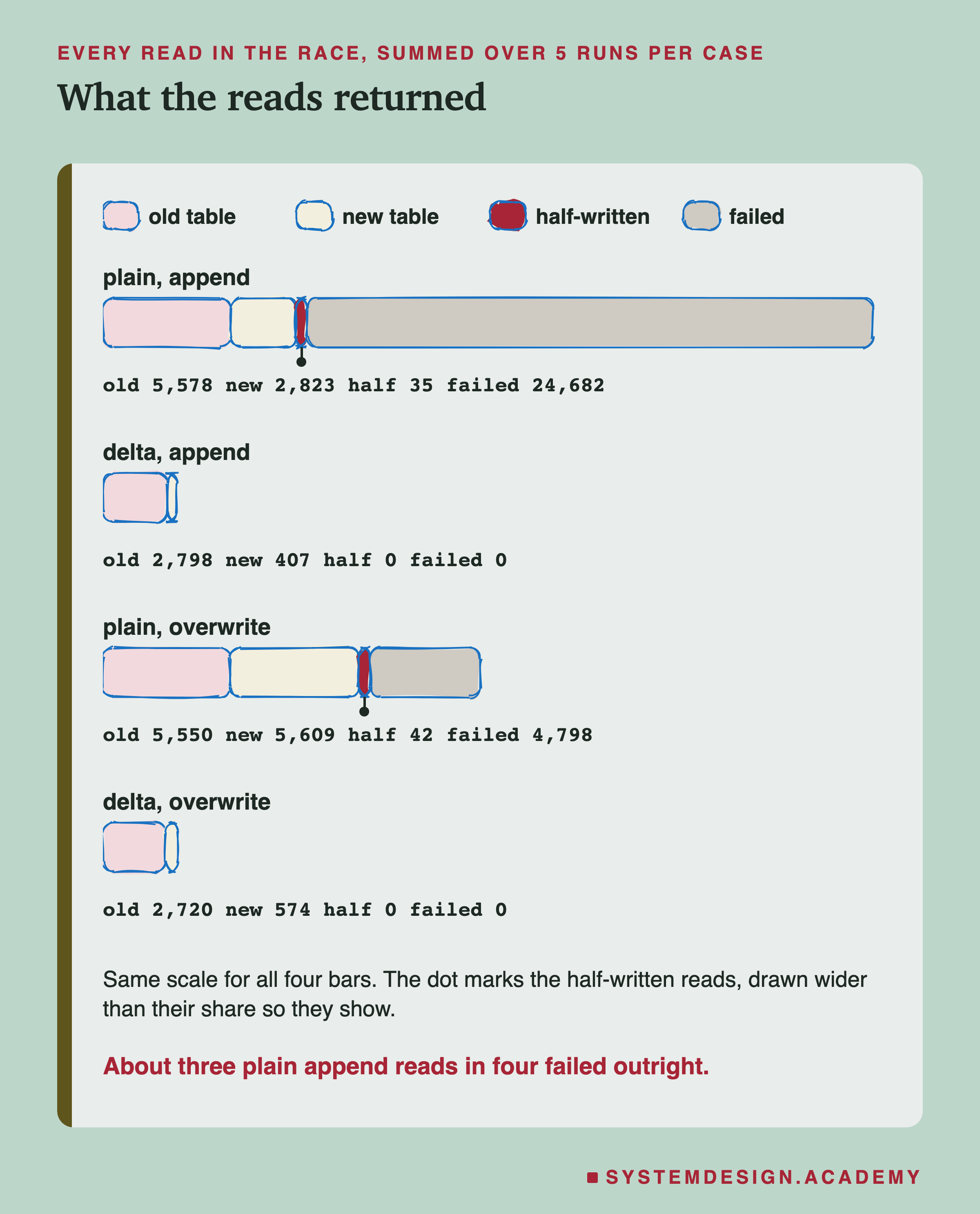
Every run of the plain folder showed the problem. In the append case, the reader saw 7 different half-written row counts in every one of the 5 runs, each one exactly once. In the overwrite case it saw 8 or 9 half-written reads per run, including the double-counted January. The Delta reader, across all 10 of its runs, saw only the old table or the new one: 0 half-written reads and 0 failures.

The failures surprised me more than the half tables. In the plain append runs, 4,847 to 5,003 reads per run did not return a number at all. That is about three of every four. They stopped with an error such as "Parquet file size is 0 bytes".

That is the footer problem from the Parquet slide. Some failed reads found a file of 0 bytes, and others found only 4 bytes, the PAR1 at the start. So pyarrow had already created the next file but had not yet written its footer. For most of the race, the folder held one file like that. In every one of the 5 overwrite runs, a second kind of failure also appeared. The reader listed a file, and the writer deleted it before the reader could read its footer.

Partly. Amazon S3 is a different kind of storage from my laptop's disk. It stores each file as one object, and its documentation makes a promise about a single object: "Updates to a single key are atomic." A reader of one object gets "either the old data or the new data, but never partial or corrupt data." So on S3, the "file size is 0 bytes" failures should not happen. An object is either fully there or not there at all.

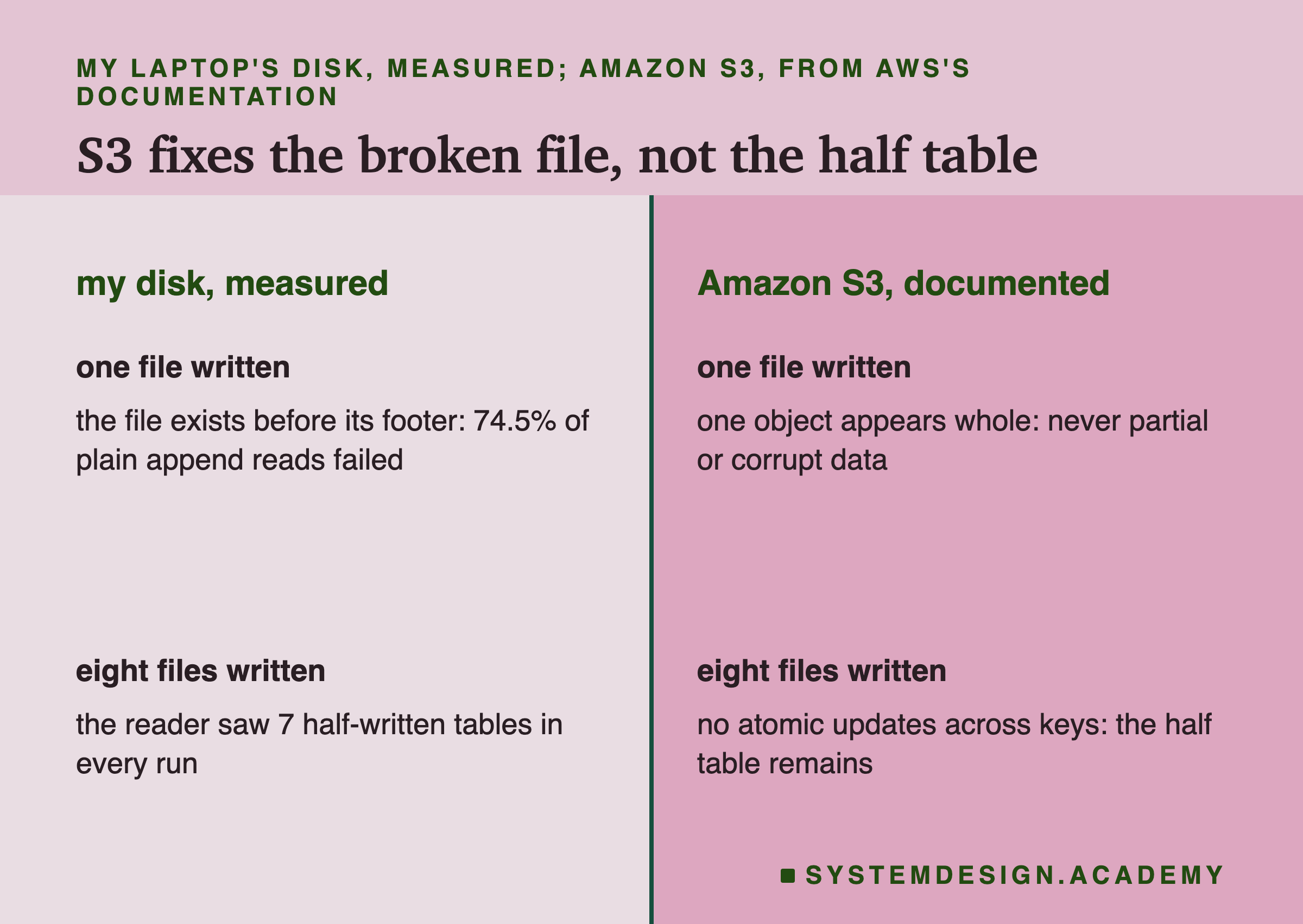
But the same page goes on: "Updates are key-based. There is no way to make atomic updates across keys." A load of 8 files is 8 separate updates. A reader that lists the bucket in the middle of them still sees some of the new files and not others. The broken-file failures go away. The half-written table, and reads that fail because a listed file was deleted, do not.

I did not run the lab on S3, so please read the right-hand column as what AWS documents, not as something I measured. The 2020 Delta Lake paper from Databricks names the same problem. It was written when S3 was still eventually consistent. In its words, "because multi-object updates are not atomic, there is no isolation between queries", and readers "will see partial updates". AWS announced on 1 December 2020 that S3 "now delivers strong read-after-write consistency automatically for all applications", but that did not make several objects change together.

For the log itself, S3 now offers conditional writes. An If-None-Match header, AWS says, "prevents overwrites of existing data by validating that there's not an object with the same key name already in your bucket". That is the put-if-absent step the commit needs. How do I know the numbers on these slides are right?

I wrote the lab's design into the docstring of scripts/labs/de-sd/lakehouse_atomicity.py before it first ran. It lists the data, the 8-file cut, the four step tests, the four race cases with 5 runs each, and my guesses about the results. It records the library versions it ran with: deltalake 1.6.6, DuckDB 1.5.6 and pyarrow 25.0.1, on Python 3.14.

One thing changed after the first run, and I want to say it plainly. In that first run, write_deltalake wrote February as 2 files, not 8. I had set its file size target from the size of the data in memory, which is much bigger than on disk. That made the race unfair: fewer files means fewer in-between moments to catch.

I changed the target to the on-disk size of one plain February file. That gave 9 files for the append and 8 for the overwrite, and I ran everything again. Every number in this lesson is from the second run. The change is written into the docstring with its date.

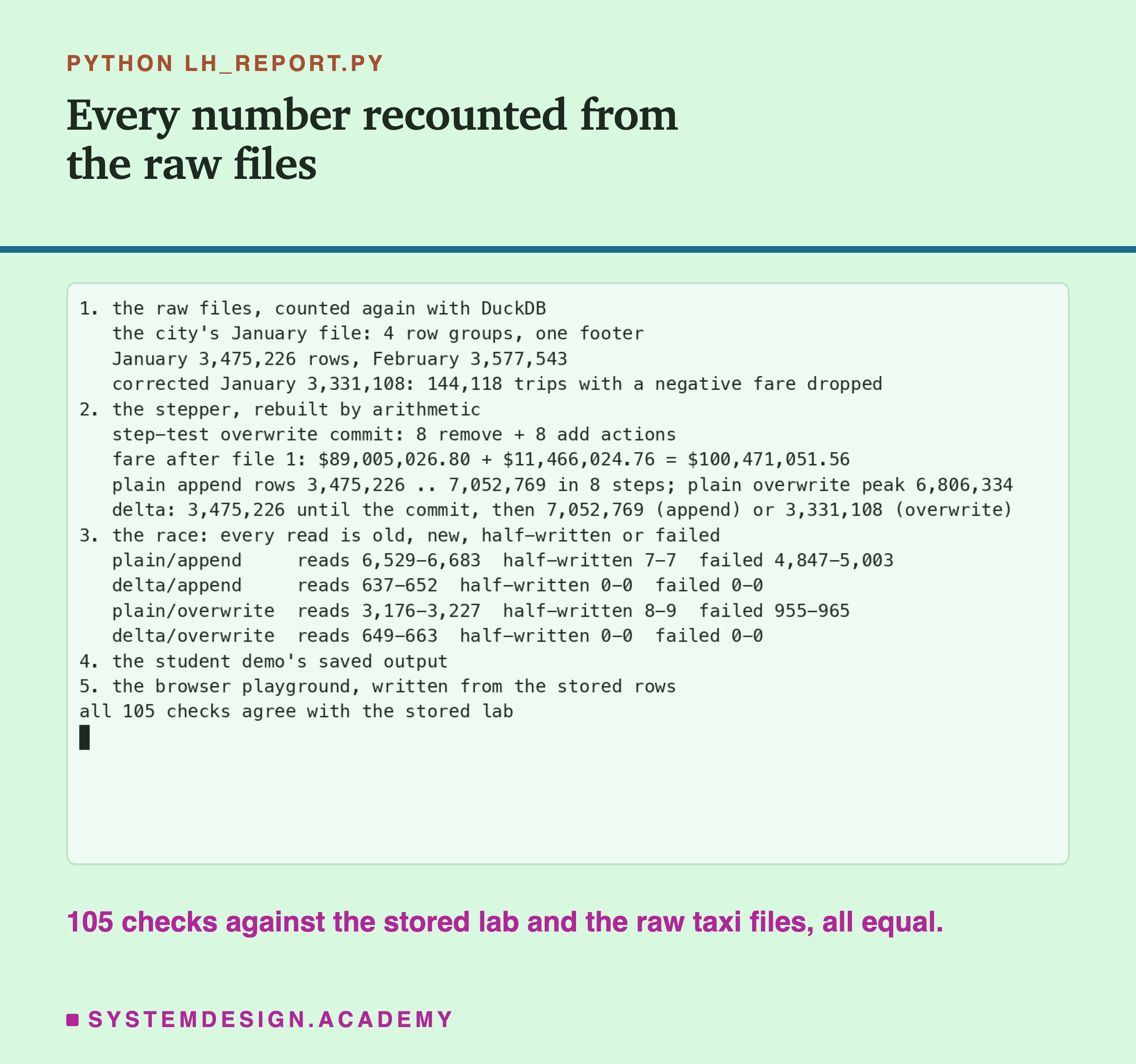
The report script, lh_report.py, does not reuse the lab's code. It counts the raw monthly files again with DuckDB, cuts them again with its own arithmetic, and works out what each reader must have seen at every step.

It checks that every race read was one of four things: the old table, the new table, a half-written table, or a failure, with nothing left over. It checks that each Delta commit holds the add and remove actions I describe, including the 8 and 8 of the step-test overwrite. It also rebuilds the fare sum after February's first file from the raw rows. I also planted a wrong number in the stored results, to see the report fail. It stopped with a mismatch and exit code 1; that run is saved as .

Before the first run, I wrote three guesses into the lab. Here they are against the results.

1. "S1/S3: the folder reader sees every in-between count (9 and 17 distinct states)." Right. The plain append showed 9 distinct row counts, and the plain overwrite 17 moments, with 17 different counts.

2. "S2/S4: the Delta reader sees 2 states only; the folder listing of the Delta table sees the uncommitted and the removed files (in S4, double the rows after the commit, until a vacuum)." Right. The Delta reader saw exactly 2 counts in both tests. A listing of the Delta folder after the overwrite counted 16 files and 6,806,334 rows.

3. "Race: plain sees in-between counts in every run and some failed reads; delta sees 0 illegal counts and 0 failed reads in every run." Right on the direction, wrong on the size. I wrote "some failed reads". In the append race, about three reads in four failed. I did not expect the footer problem to dominate the race like that.

I also did not guess one detail that the numbers show. In every plain append run, each of the 7 half-written counts was caught exactly once, no more. One possible reason, which I did not test: after pyarrow finishes one file, it creates the next empty file almost at once. So a clean in-between moment may last about as long as one read. I report it as what I saw, not as a rule.

Three guesses, three right on the main point. Now you can see the same thing on your own machine.

The full lab runs 4 step tests and 20 races. I wrote a small demo that does one slice of it: the step-by-step append, for both readers. It runs in well under a minute.

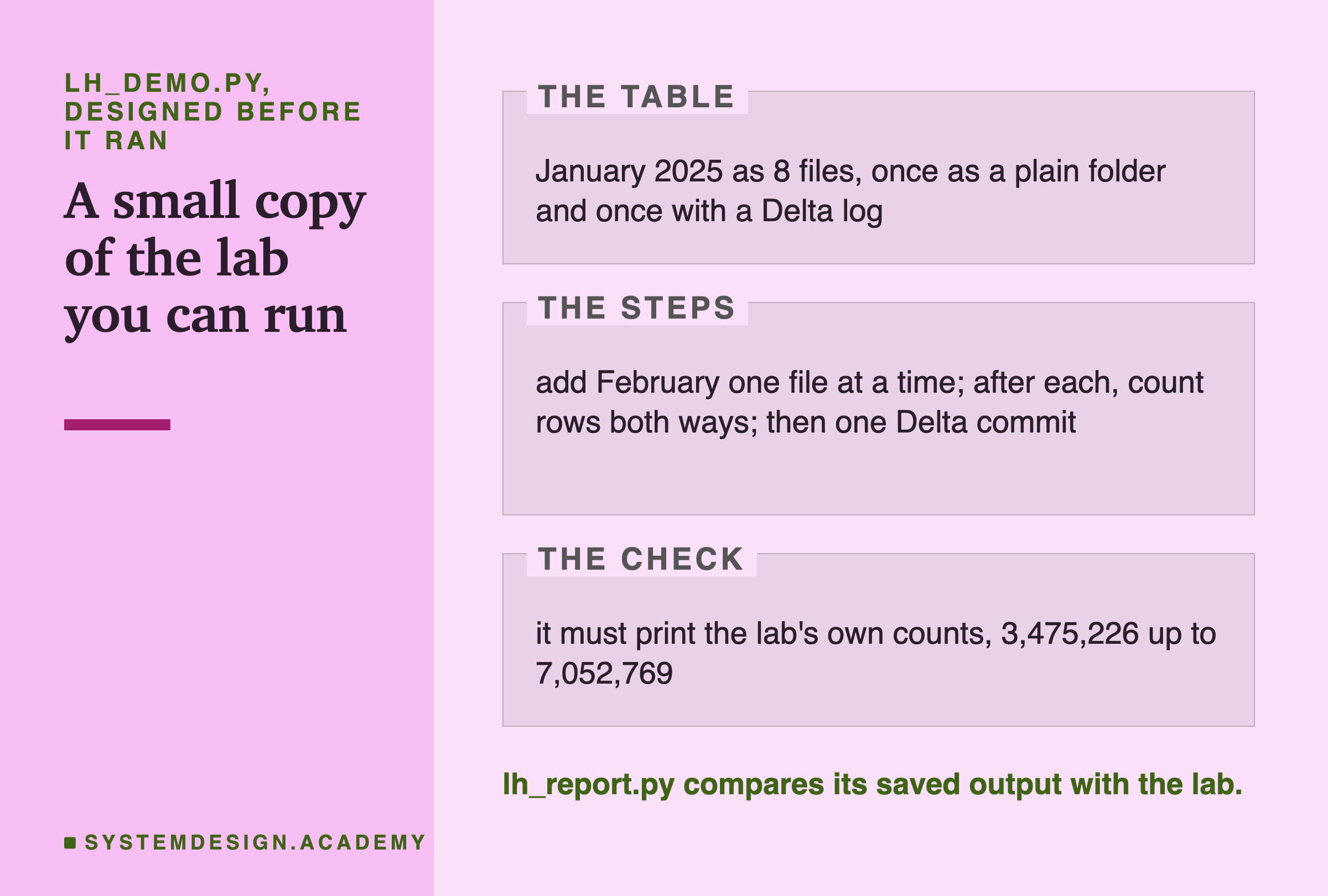
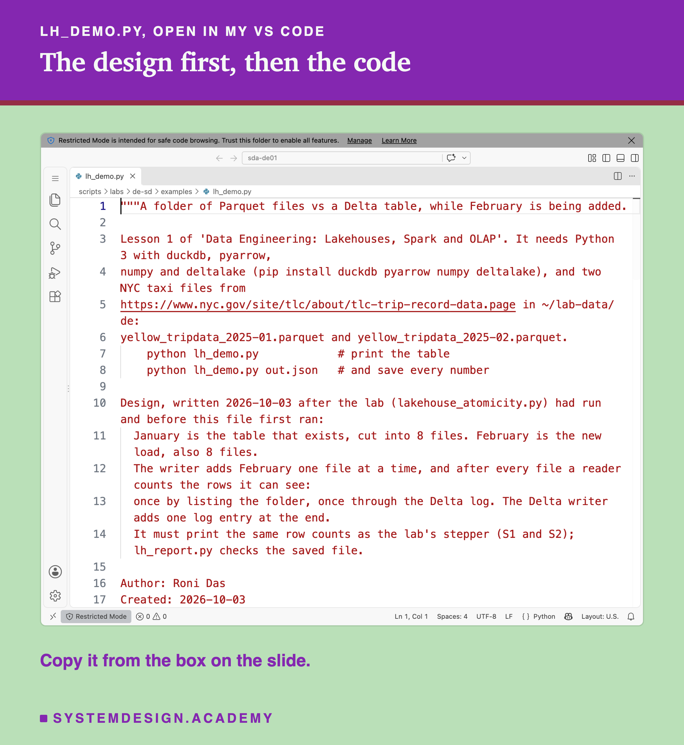
I wrote the demo's design into its docstring after the lab had run and before the demo first ran. It builds both tables in its own short way, so it is also a second check of the lab's steps S1 and S2.

Before you run this lab. You need Python 3 with four libraries: pip install duckdb pyarrow numpy deltalake. Download two monthly files of Yellow Taxi trip records, January and February 2025, from the NYC TLC trip record page. Put them in a folder called lab-data/de in your home folder. Together they are about 120 MB. The demo needs no GPU and no Java. I ran it on a Mac with the versions above. These libraries run on Windows and Linux too, but I have not checked the numbers there.

"""A folder of Parquet files vs a Delta table, while February is being added.

Lesson 1 of 'Data Engineering: Lakehouses, Spark and OLAP'. It needs Python 3 with duckdb, pyarrow,
numpy and deltalake (pip install duckdb pyarrow numpy deltalake), and two NYC taxi files from
https://www.nyc.gov/site/tlc/about/tlc-trip-record-data.page in ~/lab-data/de:
yellow_tripdata_2025-01.parquet and yellow_tripdata_2025-02.parquet.
    python lh_demo.py            # print the table
    python lh_demo.py out.json   # and save every number

Design, written 2026-10-03 after the lab (lakehouse_atomicity.py) had run and before this file first ran:
  January is the table that exists, cut into 8 files. February is the new load, also 8 files.
  The writer adds February one file at a time, and after every file a reader counts the rows it can see:
  once by listing the folder, once through the Delta log. The Delta writer adds one log entry at the end.
  It must print the same row counts as the lab's stepper (S1 and S2); lh_report.py checks the saved file.

Author: Roni Das
Created: 2026-10-03
"""
import glob
import json
import shutil
import sys
import time
from pathlib import Path

import duckdb
import numpy as np
import pyarrow.parquet as pq
from deltalake import DeltaTable, Schema
from deltalake.transaction import AddAction, create_table_with_add_actions

DATA = Path.home() / "lab-data/de"
WORK = DATA / "demo-lh"


def eight_files(month):
    t = pq.read_table(DATA / f"yellow_tripdata_2025-{month}.parquet")
    return [t.slice(int(c[0]), len(c)) for c in np.array_split(np.arange(t.num_rows), 8)]


def write(table, folder, name):
    pq.write_table(table, folder / name)
    now = int(time.time() * 1000)
    return AddAction(path=name, size=(folder / name).stat().st_size, partition_values={},
                     modification_time=now, data_change=True,
                     stats=json.dumps({"numRecords": table.num_rows}))


def folder_rows(folder):
    files = glob.glob(str(folder / "*.parquet"))
    return duckdb.sql(f"select count(*) from read_parquet({files!r})").fetchone()[0]


def delta_rows(folder):
    return DeltaTable(str(folder)).to_pyarrow_dataset().count_rows()


jan, feb = eight_files("01"), eight_files("02")
if WORK.exists():
    shutil.rmtree(WORK)
plain, delta = WORK / "plain", WORK / "delta"
plain.mkdir(parents=True)
delta.mkdir()

for i, t in enumerate(jan):
    write(t, plain, f"jan-{i}.parquet")
actions = [write(t, delta, f"jan-{i}.parquet") for i, t in enumerate(jan)]
create_table_with_add_actions(str(delta), Schema.from_arrow(jan[0].schema), actions)

out = {"plain": [folder_rows(plain)], "delta": [delta_rows(delta)]}
print(f"{'moment':28s} {'folder reader':>14s} {'Delta reader':>14s}")
print(f"{'January only':28s} {out['plain'][-1]:>14,} {out['delta'][-1]:>14,}")
new = []
for i, t in enumerate(feb):
    write(t, plain, f"feb-{i}.parquet")
    new.append(write(t, delta, f"feb-{i}.parquet"))
    out["plain"].append(folder_rows(plain))
    out["delta"].append(delta_rows(delta))
    print(f"{f'February file {i + 1} of 8 written':28s} {out['plain'][-1]:>14,} {out['delta'][-1]:>14,}")
DeltaTable(str(delta)).create_write_transaction(new, mode="append", schema=jan[0].schema)
out["delta"].append(delta_rows(delta))
print(f"{'Delta log entry committed':28s} {'':>14s} {out['delta'][-1]:>14,}")
shutil.rmtree(WORK)
if len(sys.argv) > 1:
    Path(sys.argv[1]).write_text(json.dumps(out))

This box holds the real row count of every one of the 16 files from the lab. It needs nothing but Python, so it runs in your browser. It does not read any real files. It adds up the stored counts the way each reader would.

Press Run. With the settings as they are, the writer has finished 3 of February's 8 files and has not committed. The folder reader counts January plus three February files, a half-written table. The Delta reader counts January only. Then try WRITTEN = 8 and COMMITTED = True, and both readers agree on the new table. Try COMMITTED = True with fewer than 8 files, and the box tells you the writer will not commit yet.

The report script checks that the file counts in this box are exactly the stored ones from the lab.

The lab is one file, scripts/labs/de-sd/lakehouse_atomicity.py. Here is what each part does.

split cuts a month into 8 slices of nearly equal row counts, by row position. write_files saves each slice as its own Parquet file and returns the file name, its row count and its size. add_actions turns that list into Delta add actions, each with its row count in the stats.

folder_view is the plain reader. It lists every *.parquet file in the folder and asks DuckDB for count(*) and the sum of total_amount over exactly those files. delta_view is the Delta reader. It opens the table with DeltaTable, which reads the log, and counts only the files the log names.

stepper runs the four step tests. For Delta, it writes the data files itself and then calls create_write_transaction to add the one log entry. That splits the two phases a normal write_deltalake call runs inside, so the reader can look between them.

So far: a table that is a folder shows readers every half-written moment, and a table that is a log shows them only whole versions. These are the steps I would take on a real data platform, in order.

1. Never let a reader list the data folder. Every reader goes through the table's log, by using a library or engine that understands the format. In this lab, the one wrong number that survived the Delta commit, 6,806,334 rows, came from listing a Delta folder by hand.

2. Write a change as one commit. If a load writes 8 files, all 8 go into one log entry. Eight small commits would give readers seven in-between versions, which brings back the half table in a new form.

3. Replace data in the same commit that removes it. An overwrite is one entry with its remove and add actions together, never "write new, then delete old" as two jobs.

4. Keep old files long enough. Readers that started on an old version need its files until they finish. Do not shorten the vacuum waiting period to save storage unless you know no reader runs that long.

5. If you must use a plain folder, write somewhere else first. Write the new files into a separate folder, and switch readers to it in one step, for example by changing one pointer file. That is a small, home-made log, and it is better than none.

6. Test with a reader running. A load job that passes its own checks can still show half its work to a dashboard. My lab's race is two short Python functions; a test like it fits in any pipeline.

Use a lakehouse table when more than one program reads the data while it changes. That covers almost every shared table. Think of a dashboard that refreshes every few minutes, analysts running queries all day, and a model training job at night, all reading tables that loading jobs change.

Use a lakehouse table when you need to fix or replace data. An overwrite on a plain folder showed double counts here. A log turns the fix into one step, and you can go back to the old version if the fix was wrong.

A warehouse is still a good choice when your data fits its strict tables and the team works in SQL, the standard language for asking a database questions. It also suits a team that prefers to pay for a managed product over running files and logs itself. The warehouse makes the same promises inside its own storage.

A plain folder of Parquet files is fine when nothing reads while anything writes. For example, a one-off export that you write once and then only read, or files that one script writes and the same script reads later. With no reader in the middle, there is no middle to see.

Do not use a lakehouse format as a way to avoid design work. A log stops half-written reads. It does not check that the numbers are right, and it does not choose good file sizes. It also does not replace a data catalog, which tells people what the tables mean.

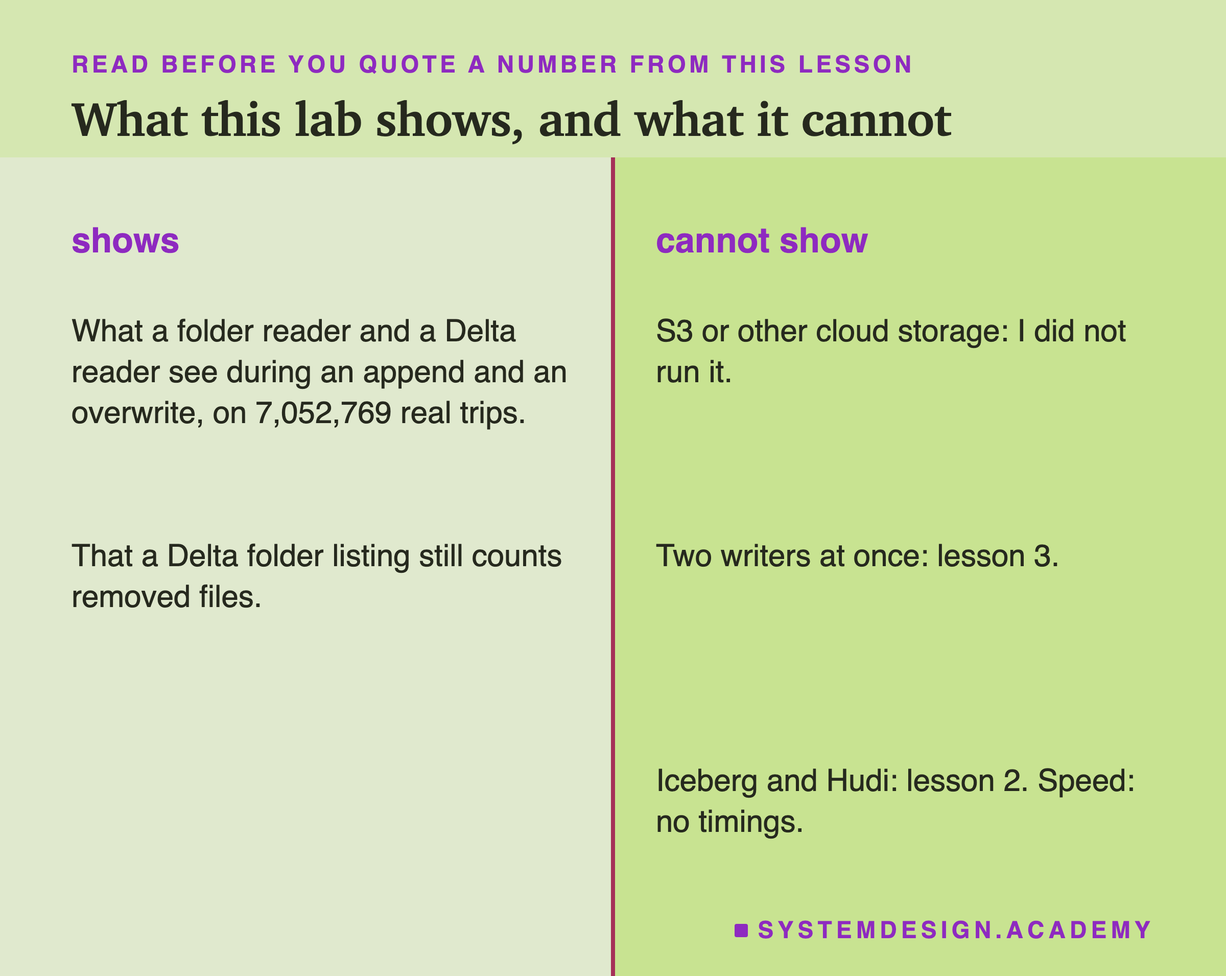
One machine, one disk. Everything ran on my laptop's own disk. Cloud storage works differently, as the S3 slide explains from AWS's documentation. The half-written tables should still appear there, because the documentation says several objects never change together, but I did not measure it.

One writer. Every test here had one writer and one reader. Two writers changing the same table at once is a different problem, with its own failure, and lesson 3 of this chapter measures it.

One format. I tested Delta Lake through the deltalake library. Apache Iceberg and Apache Hudi solve the same problem with their own logs. Their documentation says Iceberg replaces one metadata file "with an atomic swap". Hudi records every change in "a log of all actions performed on the table". Lesson 2 opens both up. I did not test them here.

The race depends on timing. The number of half-written and failed reads in a race depends on how fast each program runs, and the machine was busy. So read the race counts as "it happened in every run", not as a rate you would see elsewhere. The step-by-step test does not depend on timing at all, and it is the main evidence.

Two ways to commit. I made the step-by-step Delta commit with create_write_transaction, so I could pause between the two phases. In the race, the writer used the normal write_deltalake call, which runs the same two phases without a pause.

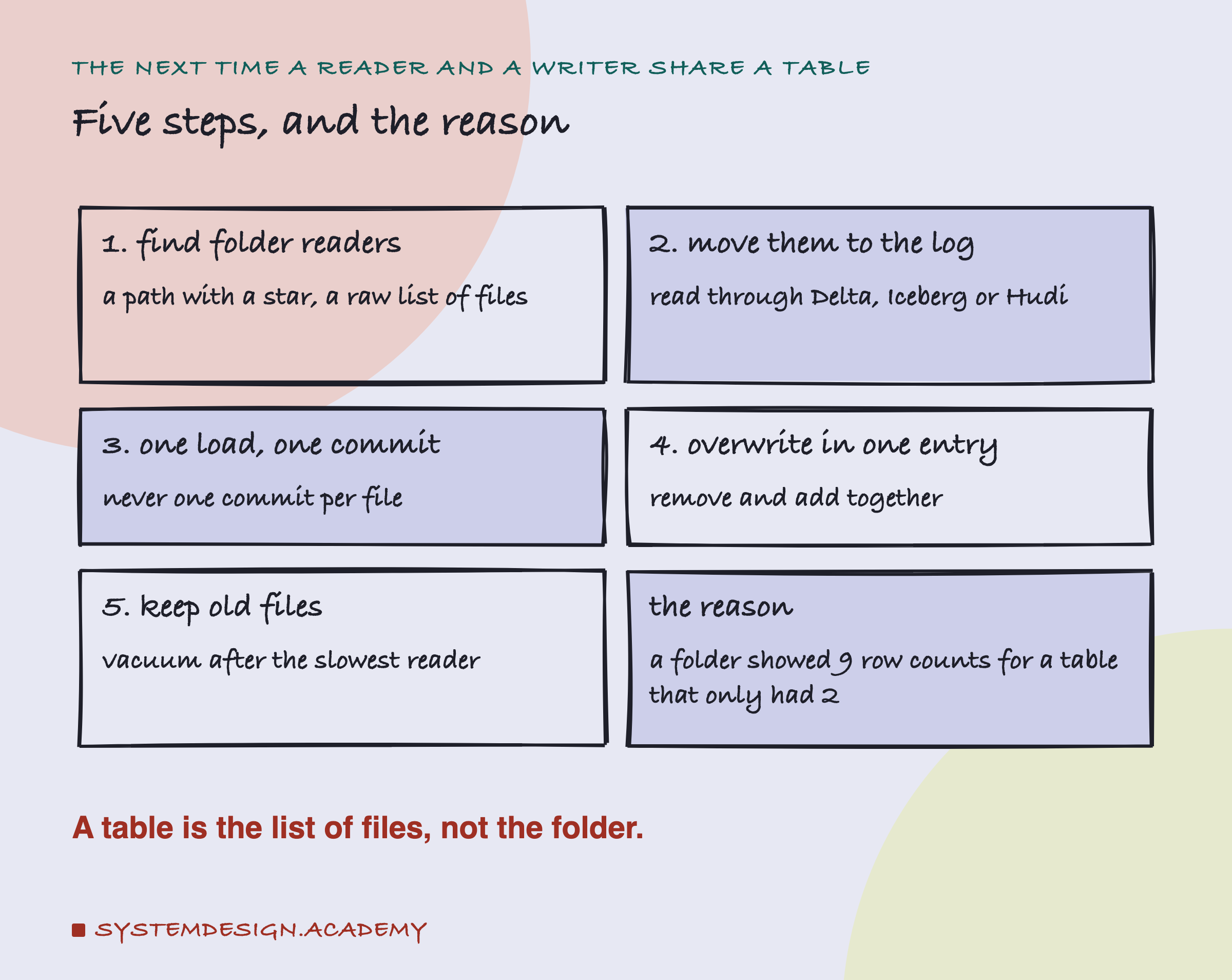
If you take one thing to work on Monday, make it this. Search your code for any reader that builds its table from a folder listing. Look for a path with a star in it, such as trips/*.parquet, or a loop over the files in a bucket. Each one can see a half-written table on any day a writer runs at the same time. In this lab, that happened in every single run.

Then move those readers to the log, one by one, starting with the dashboards people make decisions from. The writer side usually needs less work: a library like deltalake already writes one commit per call.

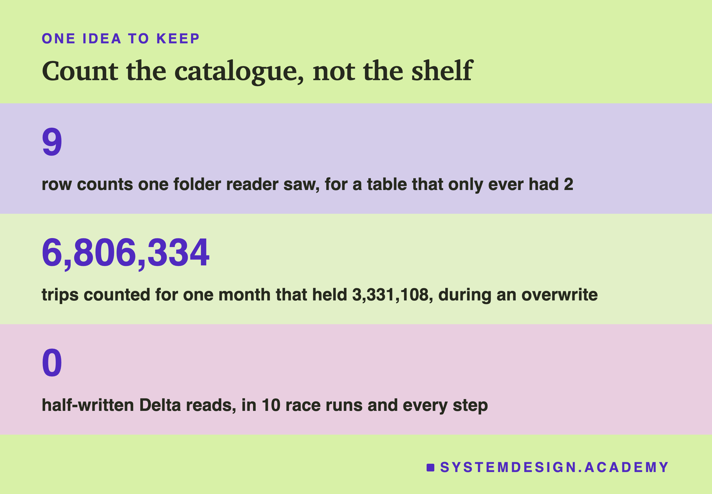
The one idea to keep: in a lake, a table is whatever a reader finds in a folder, so a reader can find a table that never existed. A lakehouse makes the table a list, and changes the list in one step. Count the catalogue, not the shelf.