Imagine a shop that keeps a box of papers for every day it has been open. The boxes go into a back room. Boxes are cheap and the room is big, so the shop keeps every one of them, going back years.

One day the owner asks a simple question: what did we sell last year? Someone goes into the back room and starts pulling out boxes. Some are labelled well and some are not. Two people filled one box at the same time, and nobody can tell whose papers are whose. One box has its numbers written 15,58 where everyone else writes 15.58. An answer comes back, and nobody trusts it.

So the shop puts a small notebook at the door. Every time a box goes in or out, one line goes into the notebook: which box was added, and which was taken away. The notebook also says what a box must look like, and the person at the door turns away a box that does not fit. Now "last year's list" has an exact meaning. Read the notebook up to the last line written on 31 December, and take exactly the boxes it names.

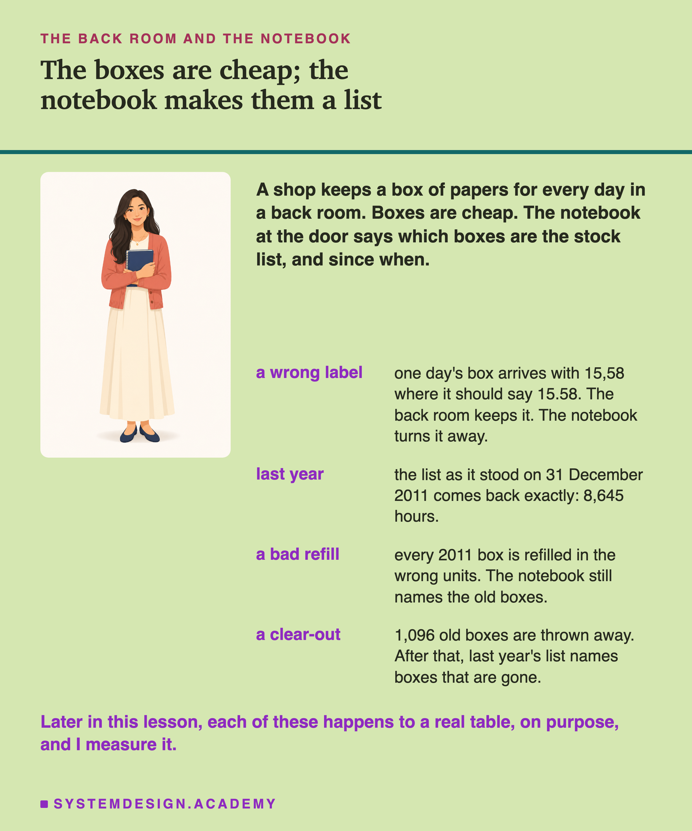
The boxes did not change, and neither did the room. The notebook turned a room full of boxes into a list you can trust. It is also a list you can ask for as it was on any day. There is one catch, in the last row of the picture. Someone tidying the room throws out the boxes the notebook no longer names. After that, an old list can name boxes that are gone.

This lesson is about the same setup in a data platform. The boxes are files of data. The back room is cheap storage. The notebook is a small log that turns a folder of files into a table. The four rows in the picture are real: later in the lesson I made each of them happen to a real table, and measured what it did.

The previous lesson, ETL vs ELT, was about when data gets cleaned: before it is loaded, or after. This lesson is about where the data sits while a model waits to learn from it. There are three common answers. A warehouse is a database that keeps clean tables for fast questions. A lake is cheap storage that keeps files exactly as they came. A lakehouse keeps the lake's files and adds the notebook from the first slide.

A model needs two things from the place its data sits. It needs a lot of data, cheaply, going back a long way. And it needs the same rows back later: the rows it learned from, exactly, when someone asks why it made a decision. The three answers give those two things in different amounts, and the lesson compares them.

The lesson has two halves. The first half explains the ideas. The first version of this lesson stopped there. For this version I checked every claim in it against the tools' own pages, their price lists and two papers, and fixed or cut what did not hold. The biggest fix was about money. The old version said a warehouse is expensive because its storage costs far more per terabyte, and the price lists say otherwise. The claims, sources and verdicts are in the lab folder, in scripts/labs/dataeng/results/lh-factcheck.json.

The second half measures. I took one real table and stored it twice: as plain files, and as files with a log. Then I did to both what a real year does to a table. A file arrived in the wrong shape. A job rewrote a year of history in the wrong units. Someone tidied up. For each event I asked what each store let me get back, and what it cost in bytes.

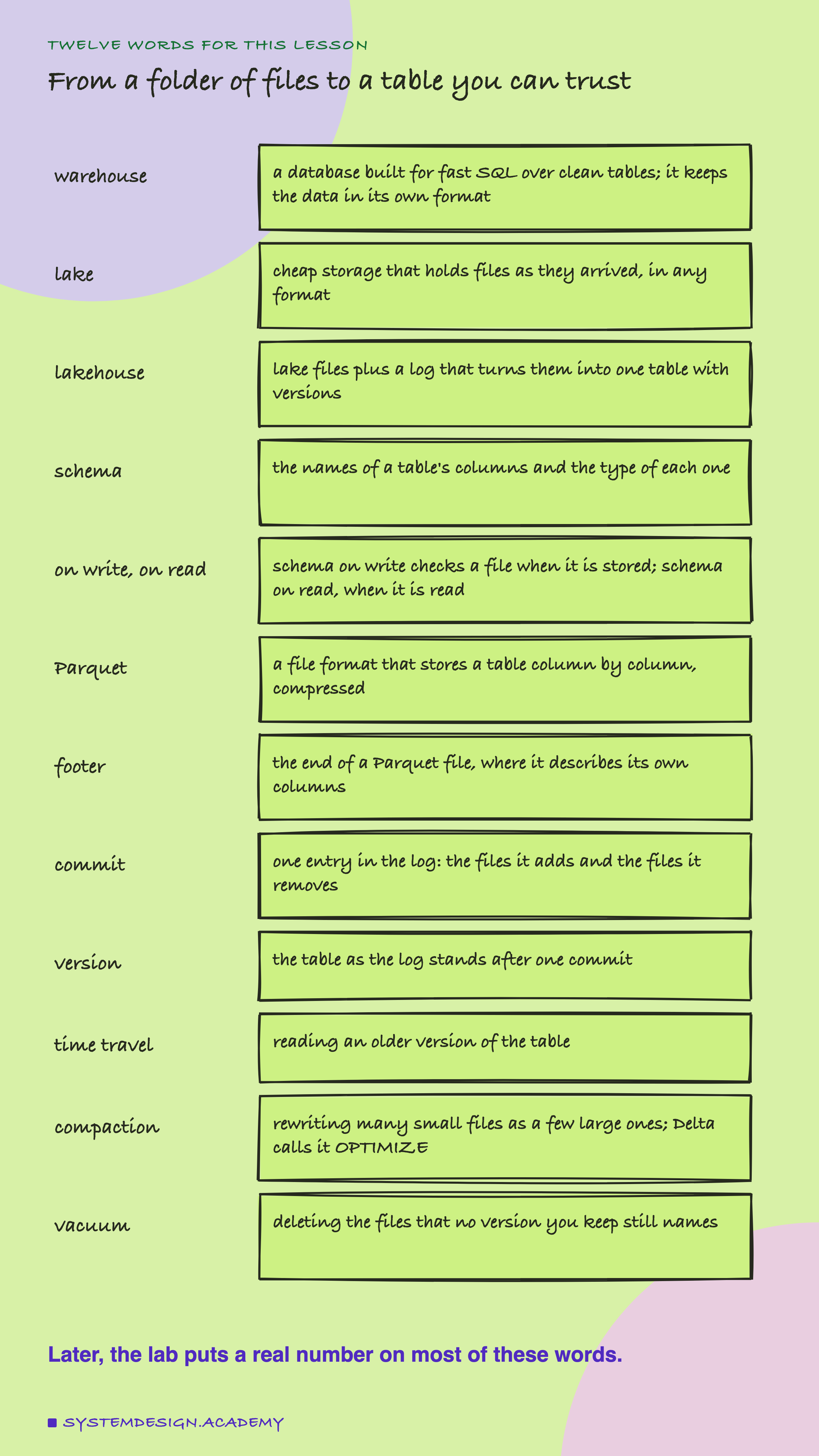
A warehouse is a database built for fast SQL over clean tables. SQL is the language most databases answer questions in. A warehouse keeps its data in its own format. A lake is cheap storage that holds files as they arrived, in any format. A lakehouse is lake files plus a log that turns them into one table with versions.

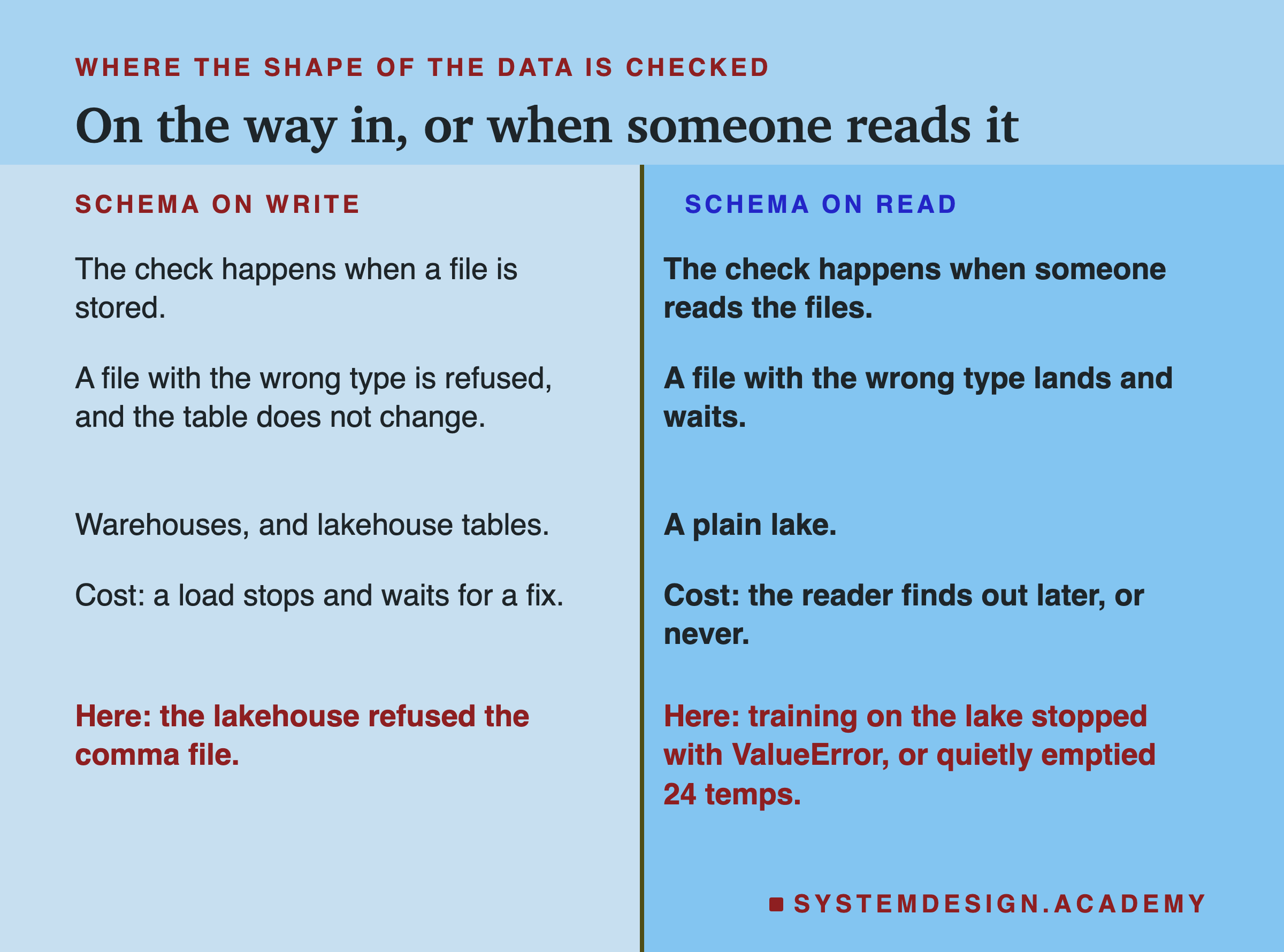
A table's schema is the names of its columns and the type of each one, such as "a number" or "text". Schema on write means the shape is checked when a file is stored. Schema on read means it is checked only when someone reads the file.

Parquet is a file format that stores a table column by column, compressed. Its footer is the part at the end of the file where it describes its own columns. CSV is the plain alternative: one line of text per row, with commas between the values.

In a lakehouse, a commit is one entry in the log: the files it adds and the files it removes. A version is the table as the log stands after one commit. Time travel is reading an older version. Compaction rewrites many small files as a few large ones; Delta Lake calls it OPTIMIZE. deletes the files that no version you keep still names.

A data warehouse is a system built for one job: fast SQL over clean, structured data. Snowflake, Google BigQuery and Amazon Redshift are the names you will meet most. Amazon's own guide calls Redshift "a fully managed, petabyte-scale data warehouse service in the cloud".

The defining trait is schema on write. You define the table's shape first. Every row you load must fit that shape, or the load stops. Think of a strict librarian at the door: nothing goes on a shelf until it is catalogued. By default both Snowflake and BigQuery stop a bulk load at the first bad row. Snowflake's COPY defaults to ABORT_STATEMENT, and BigQuery's maxBadRecords defaults to 0. Both can be told to skip bad rows, so this is a default you can change, not a law.

That strictness buys three things. Queries are fast, because the warehouse controls how the data is laid out. Snowflake's documentation says that when data is loaded, Snowflake "reorganizes that data into its internally optimized, compressed, columnar format". Data is trustworthy, because bad rows were stopped at the door, not found three steps deep in a model's inputs. And old versions are kept for a while. Snowflake's Time Travel keeps 1 day as standard and up to 90 days on its Enterprise edition. BigQuery keeps 7 days by default, and you can set anything from 2 to 7.

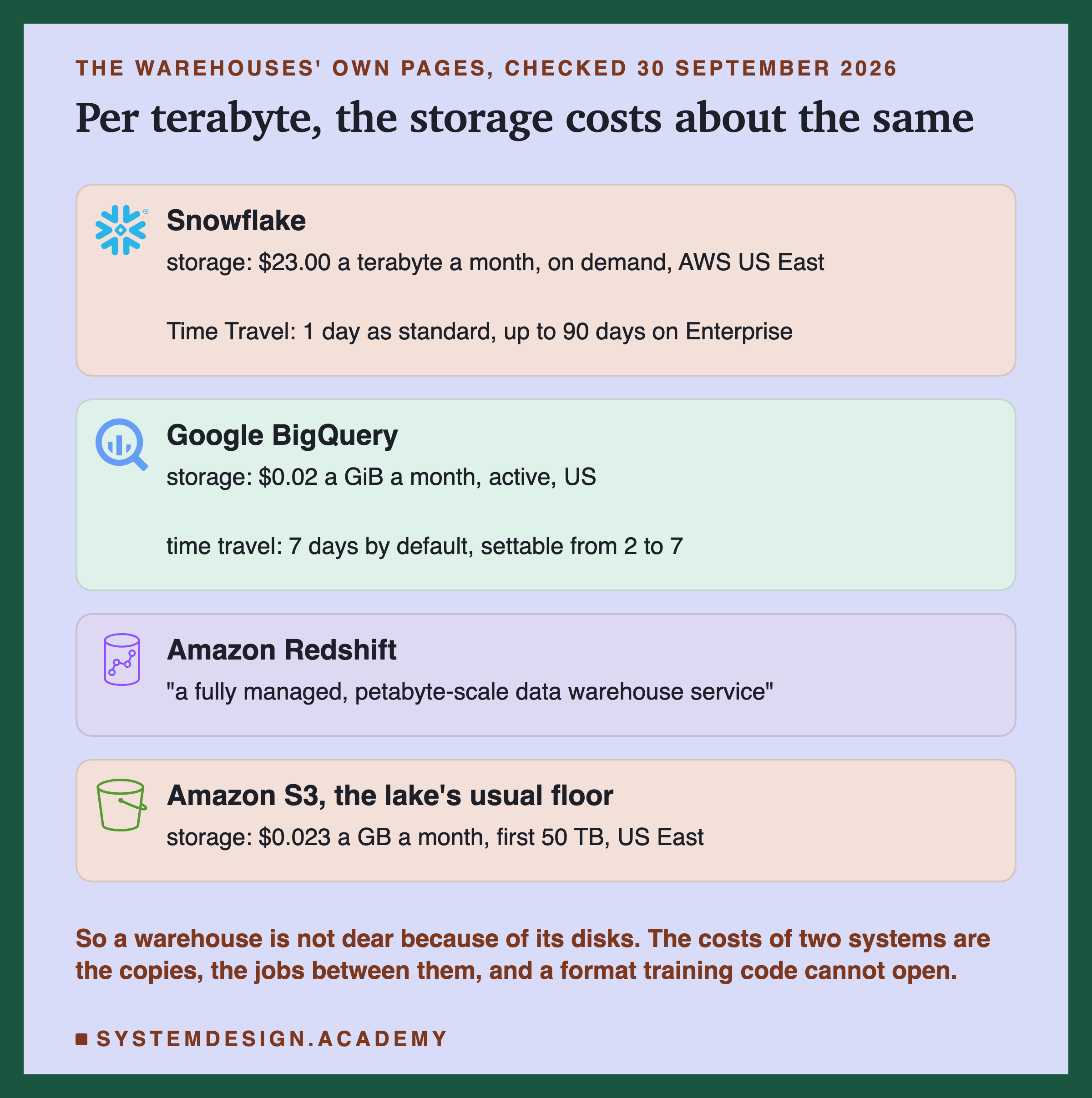
Now the claim the old version of this lesson got wrong. It said a warehouse charges "a premium per terabyte" for storage. Snowflake's own price list, effective 28 September 2026, charges $23.00 a terabyte a month on demand in AWS US East. Amazon S3, the usual floor under a lake, charges $0.023 a gigabyte a month for the first 50 terabytes in the same region. A terabyte is about a thousand gigabytes, so the two are about the same.

A data lake turns the warehouse around. Instead of a system with its own format, it is cheap object storage holding raw files in whatever format they arrived in. Object storage is a service that keeps files, called objects, and hands them back by name. Amazon S3, Google Cloud Storage and Azure Blob Storage are the big three.

The defining trait is schema on read. You store the raw bytes now and decide their shape only when something reads them. There is no librarian at the door. The boxes go straight onto the floor, to be sorted out later, if anyone ever needs them.

The economics are the point. At $0.023 a gigabyte a month, keeping years of raw history costs little. And a lake accepts anything: Parquet, CSV, JSON, images, audio, model files. So raw training data very often lives in a lake. Picture a training set of millions of images, read once a quarter by one job: a folder of files is its natural home.

But cheap and open with no rules has a failure mode, and it has a name: the data swamp. The 2020 paper that introduced Delta Lake, by Michael Armbrust and colleagues at Databricks, lists what goes wrong when a table is just files in object storage.

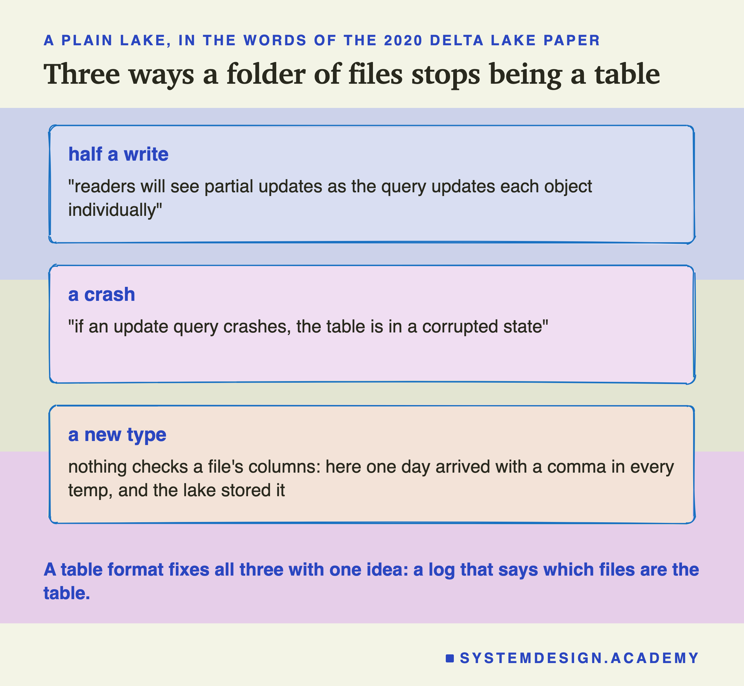
Half a write. A job that changes a table writes many files, one after another. The paper says "readers will see partial updates as the query updates each object individually".

A crash. If the job dies halfway, the paper says, "the table is in a corrupted state": some of the new files are there and some are not.

A new type. Nothing checks a file's columns. A pipeline can start writing text where there were numbers, and the lake stores it. The lab later in this lesson does exactly this, with a comma in every temperature of one day's file.

Fixing one row. Even Delta Lake's documentation says that by default, "when a single row in a data file is deleted, the entire Parquet file containing the record must be rewritten". On a plain lake you do that by hand. Delta's deletion vectors, from version 2.3.0, can mark a row deleted without the rewrite.

For years the common answer was to run both. Land everything in a lake, then copy the clean part into a warehouse for the dashboards. The 2021 paper that made the word "lakehouse" widely known calls this the two-tier architecture. Its authors are Michael Armbrust, Ali Ghodsi, Reynold Xin and Matei Zaharia, all of Databricks, and it was published at the CIDR conference.

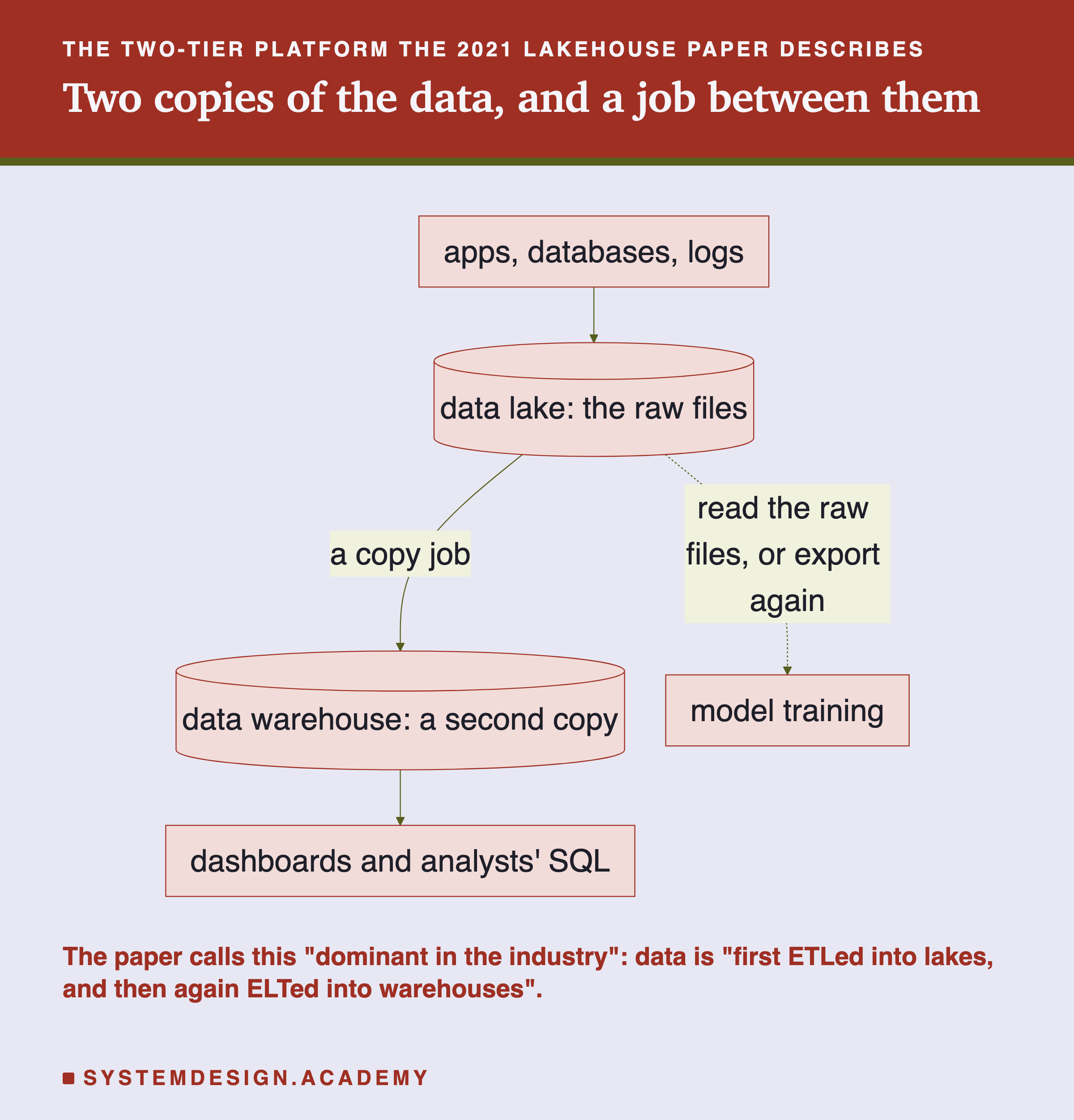
The paper says this design is "dominant in the industry in our experience (used at virtually all Fortune 500 enterprises)". Data is "first ETLed into lakes, and then again ELTed into warehouses". ETL and ELT were the last lesson: copy, clean and load, in one order or the other. The paper then lists what the second copy costs. Keeping the two consistent "is difficult and costly". The warehouse copy goes stale. And "users pay double the storage cost for data copied to a warehouse".

For machine learning the paper makes a sharper point: "none of the leading machine learning systems, such as TensorFlow, PyTorch and XGBoost, work well on top of warehouses." Those tools read large amounts of data with code that is not SQL. The paper adds that "there is no way to directly access the internal warehouse proprietary formats". So a data scientist either reads the raw lake and gets none of the warehouse's checks, or exports from the warehouse. The paper calls that export "adding a third ETL step".

Read the paper with one caution. Its authors sell the lakehouse, so this is their case for it, not a neutral survey. The problem it describes is easy to recognise, though: two copies of the truth, and a model trained on the one nobody checks. Here is the whole platform the rest of this lesson builds towards, as an interactive diagram.

The lakehouse idea is simple. Keep the lake's cheap, open files, and add a thin record on top that gives them a warehouse's guarantees. The CIDR paper's definition starts with "a data management system based on low-cost and directly-accessible storage". It then lists the database features added on top, starting with "ACID transactions" and "data versioning".

That record is an open table format. The three you will hear about are Delta Lake, Apache Iceberg and Apache Hudi. In all three, the data stays in object storage as ordinary files, usually Parquet. Beside the files, the format keeps a record of every change: which files make up the table at each version, and what its columns are.

The three keep that record in different shapes. Delta calls it a transaction log: a folder named _delta_log holding one numbered JSON file per commit. Iceberg keeps a chain of metadata files that list snapshots of the table. Metadata is data about the data: which files exist, and what their columns are. A snapshot is the table as it stood after one commit. Hudi keeps what it calls a timeline. I will call all three "the log".

Data files are never edited. To change a table, a writer first writes new files. Then it adds one entry to the log, naming the files it adds and the files it removes. The Delta Lake paper describes that last step as writing the log record for version r + 1 "if no other client has written this object. This step needs to be atomic." Atomic means all or nothing: either the entry exists, whole, or it does not exist at all.

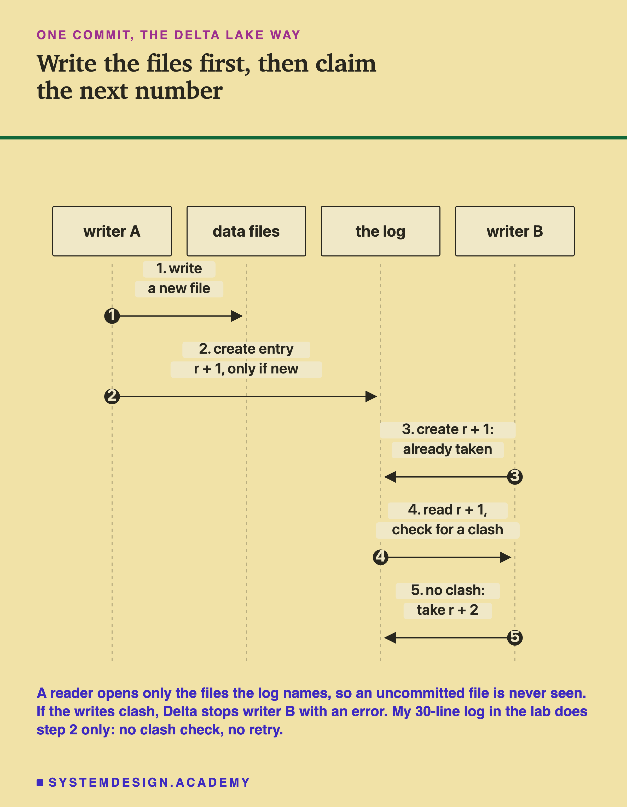
That one step gives the lake three things it never had.

ACID transactions. ACID names four promises a database makes about a change. Atomicity: it happens completely or not at all. Consistency: it leaves the table valid, schema included. Isolation: no reader sees another writer's half-finished work. Durability: once committed, it stays. Atomicity matters most here.

A lakehouse splits two things a warehouse keeps together: storage and compute. Storage is where the bytes live. Compute is the machines that run a query or a training job. In a lakehouse the data sits in object storage on its own, and engines come and go above it.

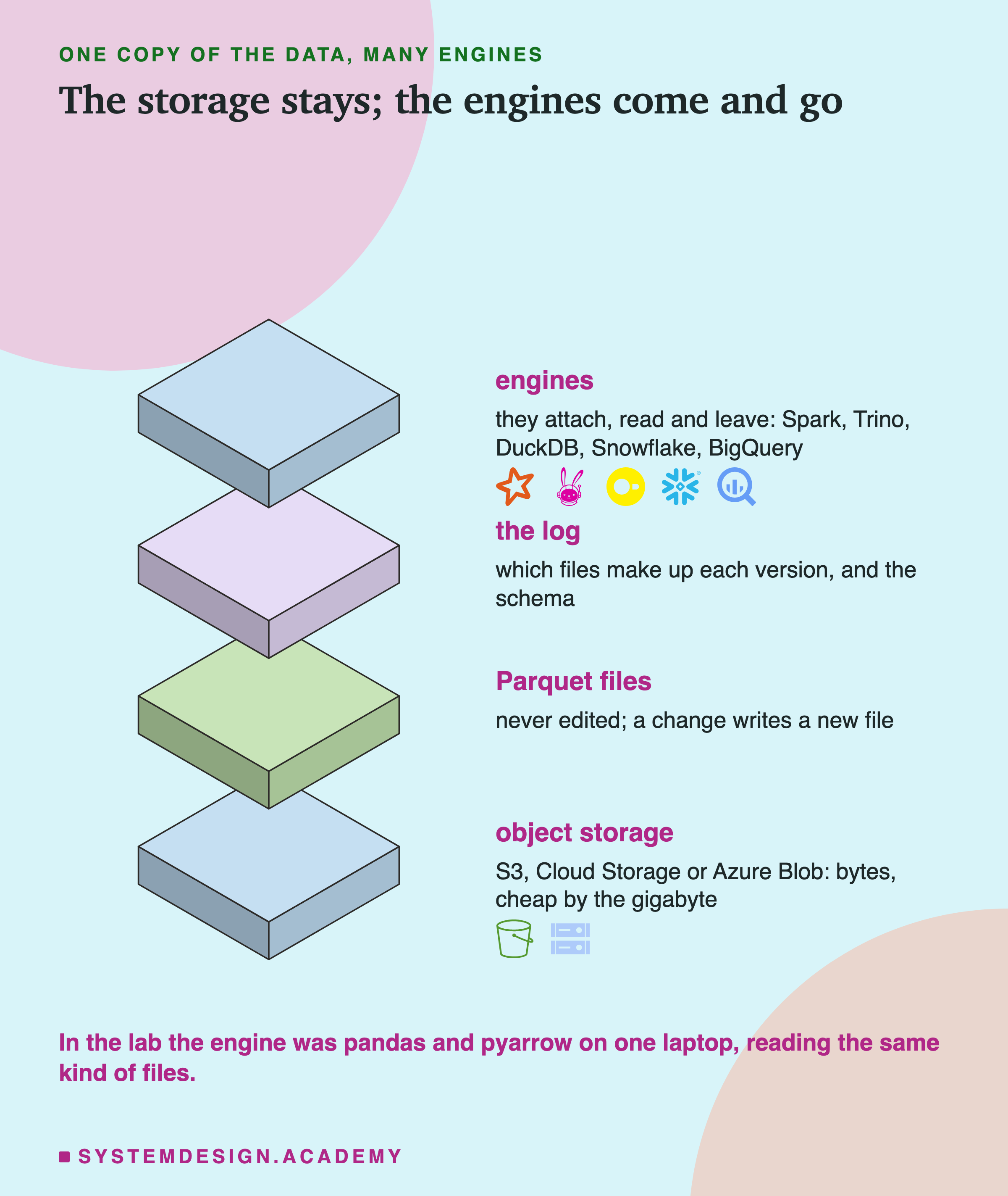
Read the stack from the bottom. Object storage holds bytes and hands them back by name. Parquet files organise those bytes by column. The log says which files make up each version, and what the columns are. At the top, engines attach, read and leave. Delta Lake's own documentation is written mostly for Spark. Trino has connectors for both Iceberg and Delta Lake, and DuckDB has extensions for both. Snowflake and BigQuery can read Iceberg tables kept in storage you manage.

You pay for storage all the time, at object storage prices. You pay for compute only while a job runs. And because no engine owns the bytes, a Spark training job and an analyst's query can read the same table without sharing one cluster. This split is also your way out of being locked in to one vendor. You can swap Spark for Trino, or add a warehouse that reads the same files, and the data never moves.

In the lab, the engine was a very small one: pandas and pyarrow, two Python libraries, on one laptop. pandas holds tables in memory, and pyarrow reads and writes Parquet. The ideas do not change with the size of the engine. What changes is how many bytes are worth reading, which the lab measures.

A lakehouse is not one pile of tables. A common discipline is to move data through three layers of quality, each its own table in the same storage. Databricks calls this the medallion architecture. Its documentation also says, fairly, that following it "is a recommended best practice but not a requirement".

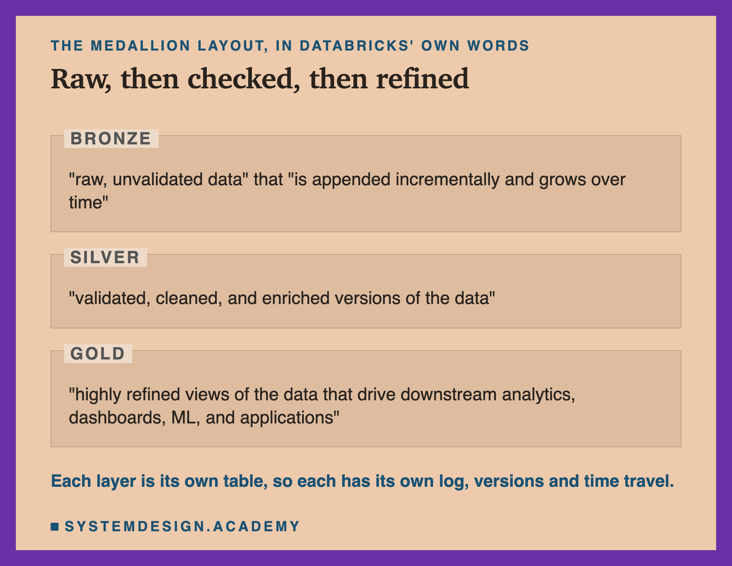
In Databricks' words, the bronze layer "contains raw, unvalidated data", and it "is appended incrementally and grows over time". Its job is not to be clean. Its job is to be complete, so that you can rebuild everything above it. If the cleaning code has a bug, you fix the code and rebuild from bronze, because the untouched source is still there.

The silver layer holds "validated, cleaned, and enriched versions of the data". This is where copies are removed, types are fixed and sources are joined. The gold layer holds "highly refined views of the data that drive downstream analytics, dashboards, ML, and applications". Databricks' page lists data scientists among the users of both silver and gold. The old version of this lesson said most machine learning inputs are built in silver; the page does not say that, so I cut it.

The point of the layout is that it adds discipline back into schema on read without giving up the lake. Raw stays raw and cheap in bronze. Structure and trust are added on purpose as data climbs. Because each layer is its own versioned table, each one can time travel.

If there is no index and the data is just files in a bucket, does every query read everything? No, and the log is why.

When an engine reads a lakehouse table, it does not list the folder and open every file. It reads the log first. The log says which files make up the version asked for, and what the columns are. It also keeps small statistics for each file. In Delta, each commit's add entry can carry a file's row count and each column's lowest and highest value. Delta collects them for the first 32 columns by default.

Two tricks follow. The first is file skipping. If a query asks for hours at 30 degrees or warmer, any file whose highest temperature is under 30 cannot hold a match, so it is never opened. The second is column pruning, which comes from Parquet. A Parquet file stores each column in its own section, called a column chunk, and describes all of them in its footer. The Parquet documentation says "readers are expected to first read the file metadata to find all the column chunks they are interested in". A query that needs 4 columns out of 14 can read just those 4.

Both are real, and the lab measured both, with my own 30-line log standing in for Delta's. File skipping worked as the documentation describes: 109 of 365 files opened, and the same 1,055 hours found as a full scan. Column pruning came with a surprise, on files this small. The single Parquet file held the model's 4 columns in 39,239 of its 98,113 bytes, yet the reader took 108,617 bytes, more than the whole file. The lab slides show why.

Notice also that a query can name a version. That is time travel, and for machine learning it is what makes a training set rebuildable. The exact rows a model learned from can be read again months later, as long as that version's files still exist.

Here is what the operations look like in Delta Lake's SQL on Spark. The point to notice is that a MERGE, which updates the rows that match and inserts the rest, commits as one change, and every version stays readable. This block comes from the first version of this lesson; I checked each statement against Delta's documentation and Spark's SQL grammar.

-- 1. Write raw events as an ACID lakehouse table on S3.
--    Under the hood: Parquet files + a _delta_log transaction log.
CREATE TABLE events
USING DELTA
LOCATION 's3://data-lake/events/'
AS SELECT * FROM raw_events;

-- 2. Nightly upsert. This whole MERGE commits atomically.
--    Readers see either the old table or the new one, never a half-written mix.
MERGE INTO events AS target
USING daily_batch AS source
  ON target.event_id = source.event_id
WHEN MATCHED THEN UPDATE SET *
WHEN NOT MATCHED THEN INSERT *;

-- 3. Time travel: read the table exactly as it was at an older version.
--    This is how a training job pins a reproducible dataset.
SELECT * FROM events VERSION AS OF 41;

-- 4. A bad load corrupted the current version? Roll back with one command.
RESTORE TABLE events TO VERSION AS OF 41;

-- 5. Housekeeping the lake needs: merge small files, then drop old ones.
OPTIMIZE events;          -- compacts many small Parquet files into fewer big ones
VACUUM events RETAIN 168 HOURS;  -- deletes files older than 7 days no longer referenced

RESTORE does not copy data back. Delta's documentation shows it as a new commit that removes the current files and adds the old ones again. It also says that "restoring a table to an older version where the data files were deleted manually or by vacuum will fail". The lab's own restore wrote no data files at all.

The last block is the tax you pay for running a lakehouse. Frequent small writes produce many small Parquet files, which slow reads down. OPTIMIZE is compaction: Delta's documentation says it improves read speed "by coalescing small files into larger ones", and it has been in open-source Delta since version 1.2.0. VACUUM deletes files that no retained version names. Iceberg has its own tools for the same jobs, rewrite_data_files and expire_snapshots. Hudi has its own too, which it calls cleaning, compaction and clustering.

The lab later in this lesson uses my own 30-line log, built the way Delta's is: a folder with one numbered JSON file per commit. Trace it on paper once: when you can replay a log by hand, time travel stops feeling like magic.

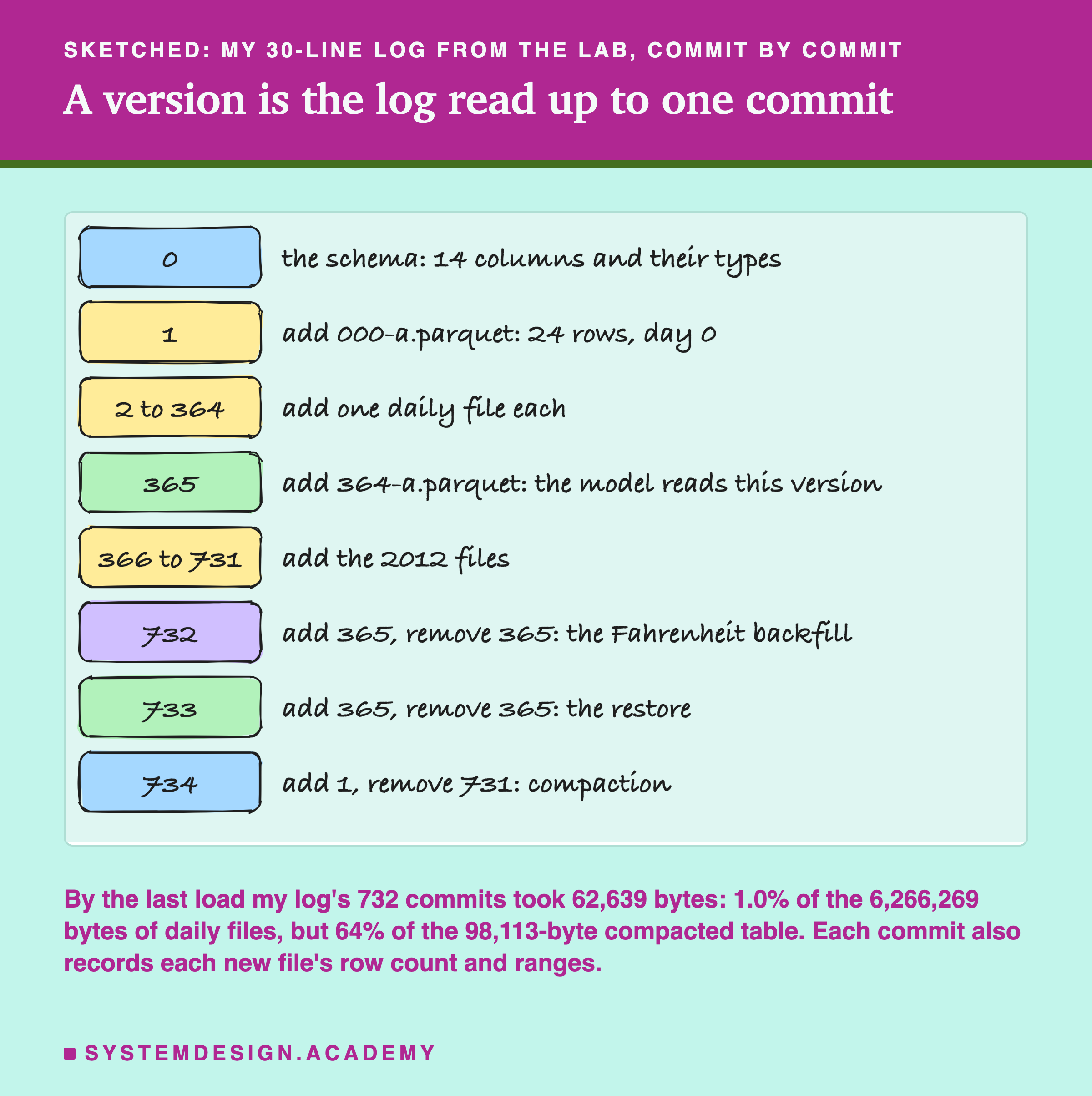
Commit 0 holds only the schema: the 14 column names and their types. Commit 1 adds the first day's file, 000-a.parquet, with its row count and its ranges. Each commit up to 365 adds one more day of 2011. The first copy of the last 2011 file was refused, so it got no version; the corrected copy became commit 365. The model learned from version 365.

To read version 365, you replay commits 0 to 365 and collect the files they add. You never look at commit 366 or later. So the pinned training set gives the same rows however many changes come after it. A version is a prefix of the log: its first entries, up to and including one commit.

Commit 732 is the Fahrenheit backfill. It adds 365 new files and removes the 365 old ones. Commit 733 is the restore: it adds the 365 old files back and removes the 365 bad ones. It wrote no data at all, because the old files were still on disk. Commit 734 is compaction: it adds 1 file and removes 731.

At the end, the storage held far more files than the latest version names. The 731 daily files and the 365 Fahrenheit files were all still there, named by old versions only. Those are exactly the files vacuum deletes. Once they are gone, replaying the log up to 365 names files that no longer exist. The same idea explains why a reader never sees a half-written table. A writer can spend minutes creating files, but readers ignore them until the one log entry that names them is written.

These are mistakes teams make when they adopt this way of storing data. The first four come from how the log works, and the lab shows several of them happening. The last comes from the price lists.

Writing to a table's folder directly. A lakehouse table is the files plus the log. If a job copies Parquet files straight into the table's folder, the log does not name them, so readers never see them. If a job deletes files by hand, the log still names them, and reads fail. Always write through the table format's own API or SQL.

Setting retention shorter than your audits need. If a model must be explainable six months later, both of Delta's windows must last six months. Those are delta.deletedFileRetentionDuration for data files, 7 days by default, and delta.logRetentionDuration for the log, 30 days by default. Raise only the first, and the version still stops reading after 30 days. In the lab, vacuum kept nothing older than the latest version, and version 365 failed with FileNotFoundError. For a very long audit, copy the training version into a table of its own.

Pinning a version but not recording it. Time travel only helps if the training run saved which version it read. Store the table version next to the model, in the same place you store the code commit.

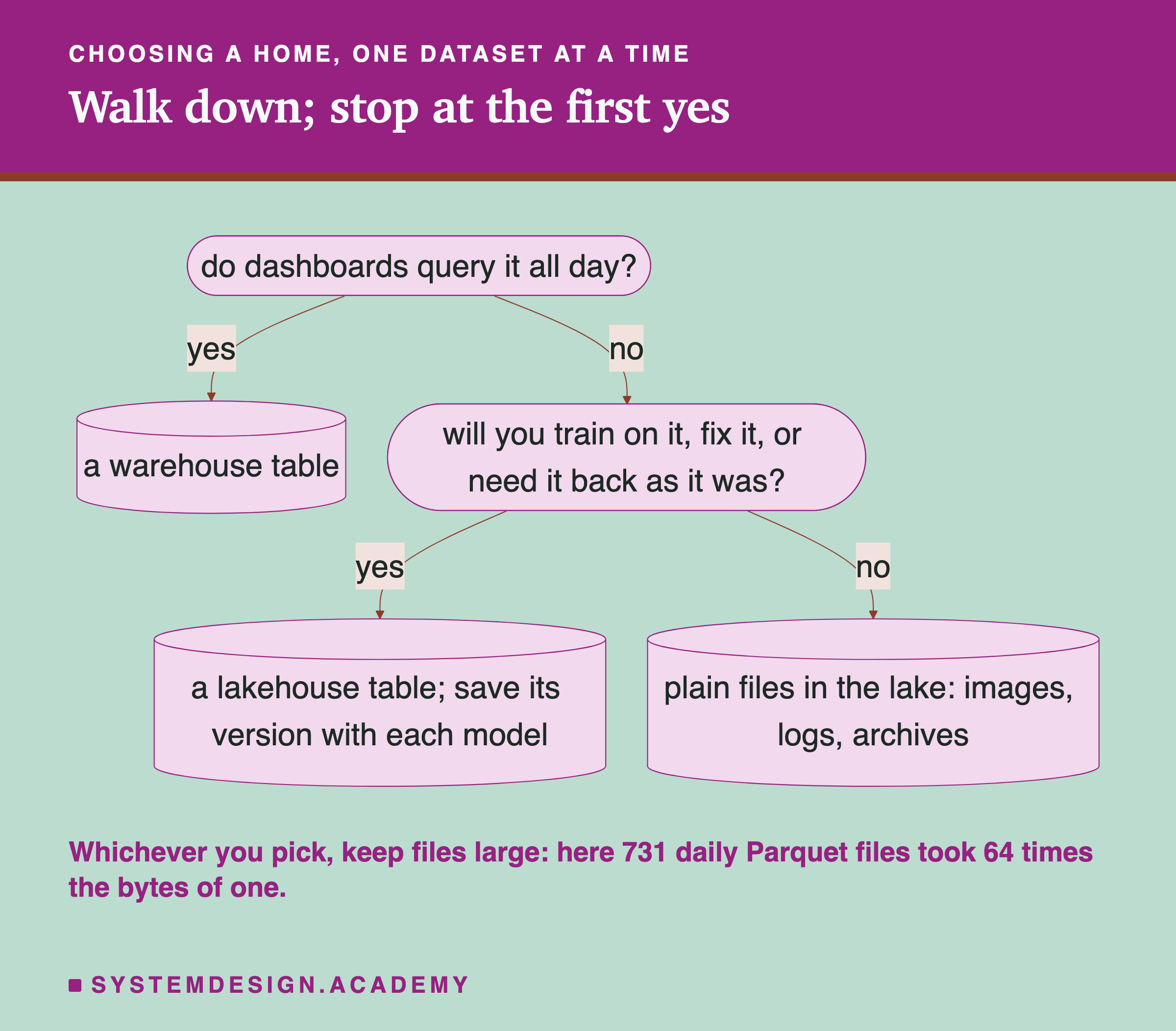
Never compacting. Many small files make every query open more files and read more of their descriptions. In the lab, 731 daily Parquet files took 64 times the bytes of the same rows in one file. Schedule compaction as a normal job, not as a fix after users complain.

Moving everything into the warehouse "to be safe". The disks cost about the same. But every row copied in means a second copy, a job to keep it fresh, and a format your training code cannot open. Keep raw files and training tables where training code can read them, and put in the warehouse only the tables dashboards hit all day.

Put the three side by side, with the facts as the vendors state them, and the difference turns out to sit somewhere unexpected. It is not the price of a disk.

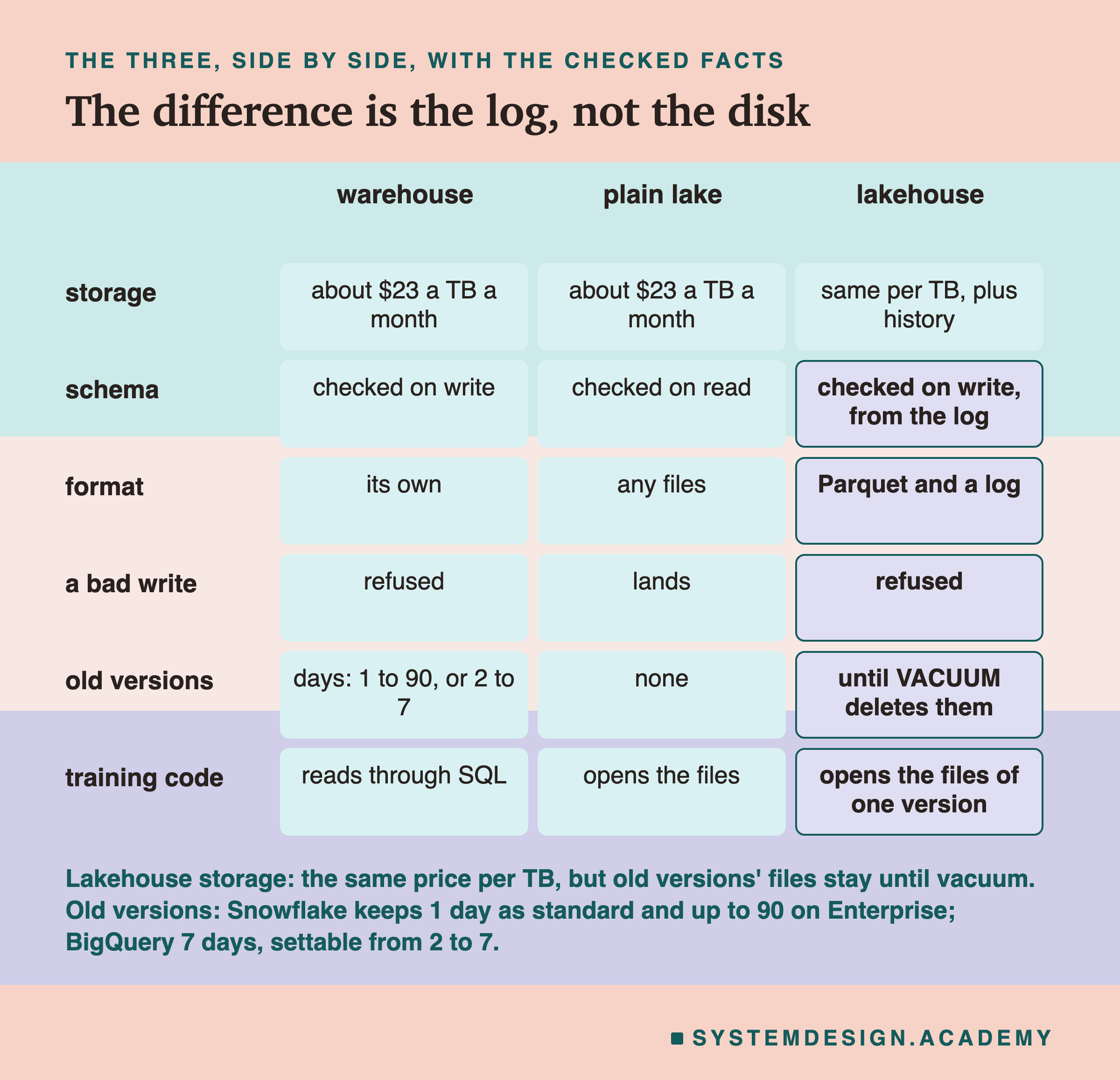
Storage costs about the same per terabyte in all three, though a lakehouse also keeps old versions' files until vacuum deletes them. The differences are in the rows below it. They are where the shape is checked, what happens to a bad write, how long old versions last, and whether training code can open the data. The lakehouse matches the warehouse on checks and keeps the lake's open files. The price is the upkeep: somebody has to run compaction and vacuum, and choose the retention.

None of this is theoretical. The three open table formats came out of three companies solving the swamp problem at scale, and their origins explain why they differ.

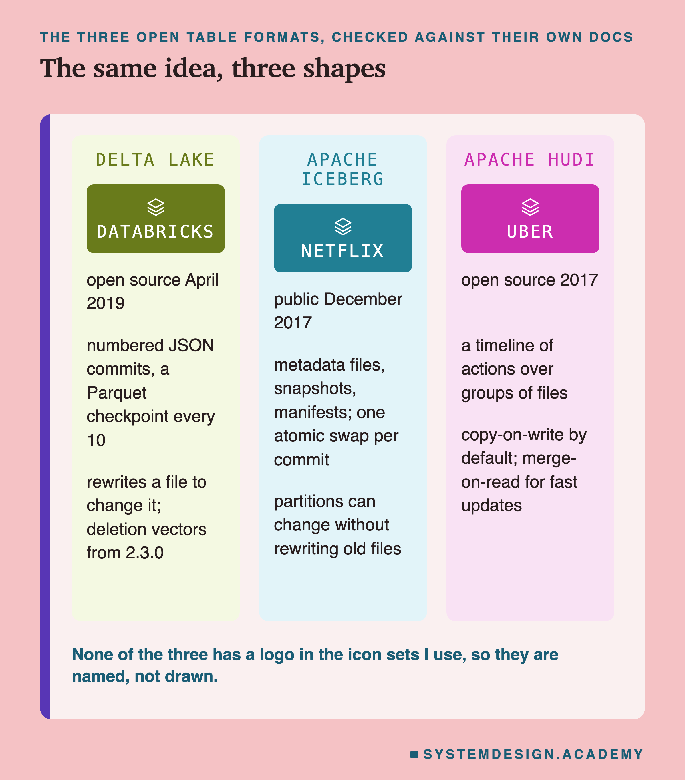
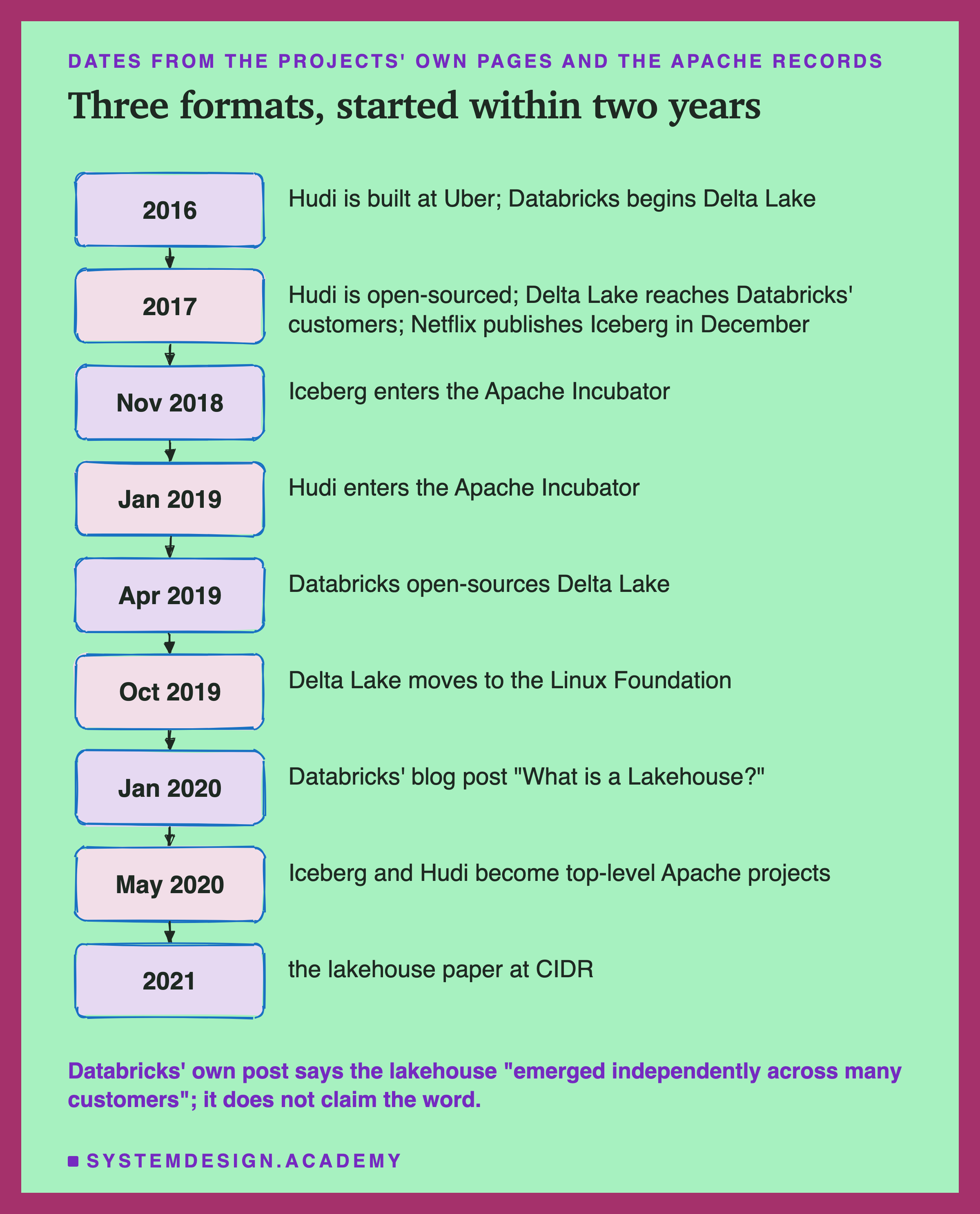
Databricks created Delta Lake. Its 2021 paper says it began building Delta Lake in 2016, and its 2020 paper that it offered Delta Lake to its customers from 2017. It open-sourced Delta Lake on 24 April 2019, and in October 2019 moved it to the Linux Foundation. Databricks' own documentation says "Delta Lake is the default format for all operations on Databricks", so if you use Databricks, you are in a lakehouse by default.

The old version of this lesson said Databricks coined the word "lakehouse". Its own January 2020 blog post does not claim that: it says the lakehouse is an architecture that "emerged independently across many customers and use cases". Databricks made the word widely known, which is a different thing.

Netflix built Apache Iceberg. The project's own page says "Iceberg was designed to solve correctness problems that affect Hive tables running in S3". Hive is an older system that tracked a table's files by listing folders. The page says that made atomic changes to a table impossible, and it also meant "many slow listing calls". Iceberg keeps a tree of metadata files instead, and each commit is one atomic swap.

Partitioning splits a table's files into groups by a column, such as one folder per day, so a query can skip whole groups. Iceberg can change how a table is partitioned without rewriting old files. Netflix published it in December 2017; it entered the Apache Incubator in November 2018 and became a top-level Apache project in May 2020.

Uber built Apache Hudi. The Apache Software Foundation's announcement spells out the name: Hadoop Upserts Deletes and Incrementals. An upsert updates a row if it exists and inserts it if not. Uber's problem was applying a constant stream of updates and deletes to huge tables, and letting later jobs read only what changed. Hudi was built at Uber in 2016, open-sourced in 2017 and became a top-level Apache project in May 2020. It offers two ways to store a table. The old version of this lesson said Hudi is "merge-on-read first". Its configuration page says the default is copy-on-write.

I wrote the lab's design at the top of its file, scripts/labs/dataeng/examples/lakehouse_demo.py, before it first ran. Every number below comes from its stored results, results/lh-demo.json. A few come from the report that rebuilds and checks them, results/lh-report.json. The parts of that report I designed after seeing the results are marked as such on each slide.

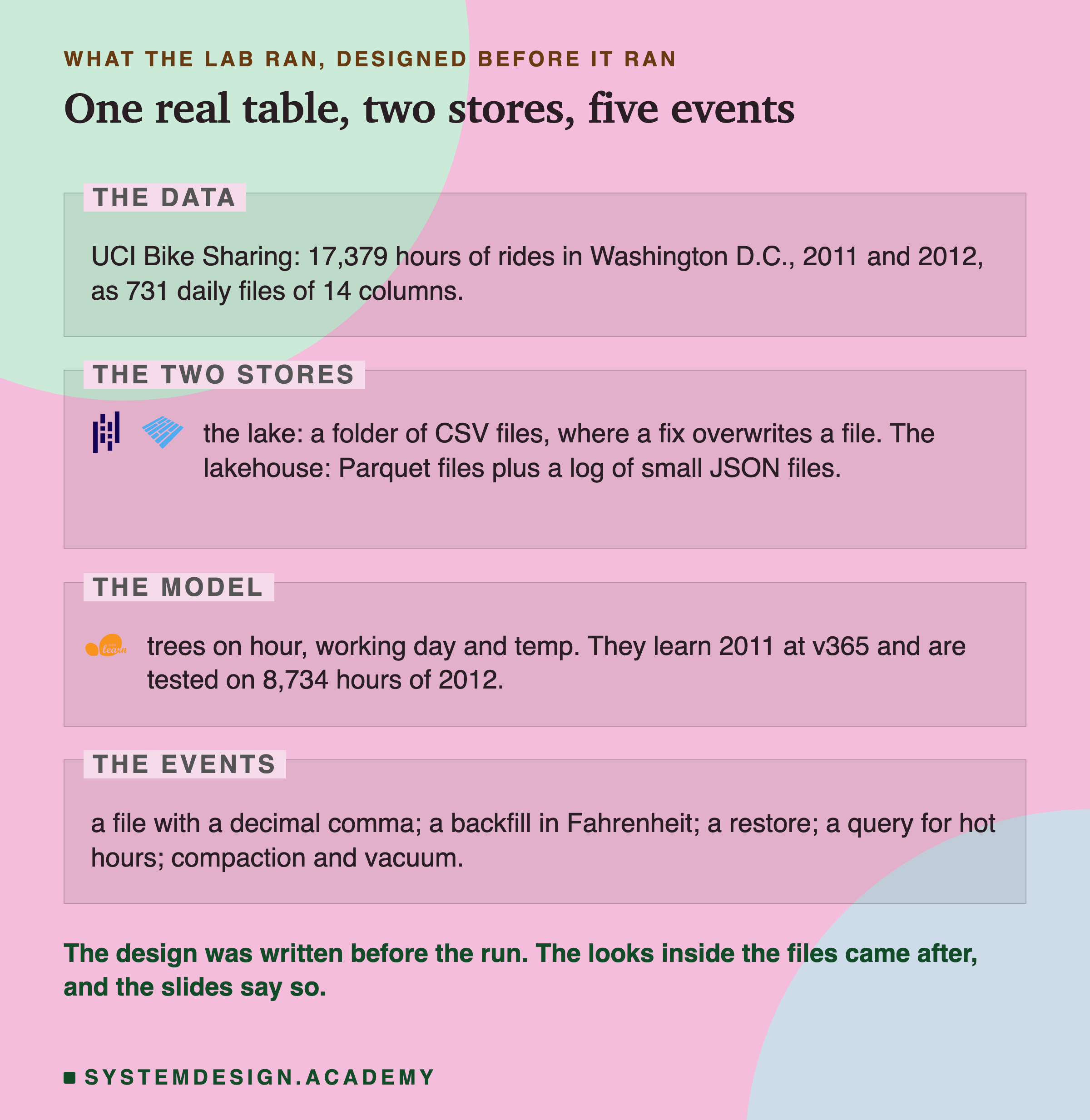
The data is UCI Bike Sharing: 17,379 hours of bike rides in Washington D.C., in 2011 and 2012, with the weather for each hour. It is small, public and real, and scikit-learn downloads it from OpenML. The file has no day of the month, so I rebuild the day from the weekday, as lesson 1 of this chapter does. That gives 731 days, each sent as one file of 14 columns.

The two stores get the same daily files. The lake is a folder of CSV files; a fix overwrites a file in place, as it would on a bare folder. The lakehouse is a folder of Parquet files plus a log, built the way Delta does it. The log holds one JSON file per commit, naming the files to add and remove. Each added file also gets its row count and its lowest and highest day and temperature. I wrote this log myself in about 30 lines, so it is Delta's idea, not Delta. A commit is written with Python's open(..., "x"), which fails if that number is already taken.

The first event came before the model ever trained. The file for 31 December 2011 arrived from an exporter that writes numbers with a comma for the decimal point, as many European settings do. So its first temperature read 15,58 instead of 15.58, and every other temperature in that file had a comma too.

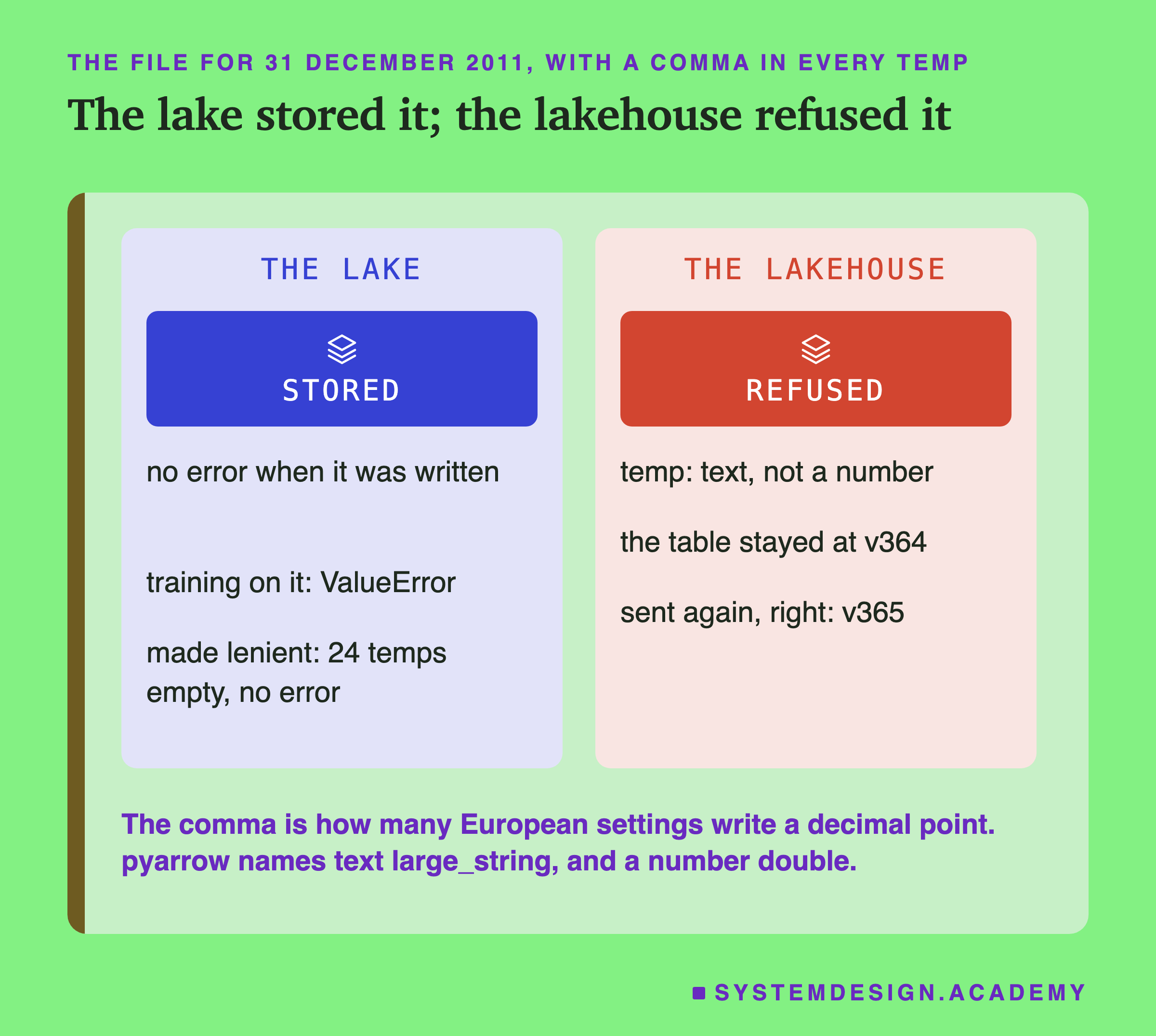
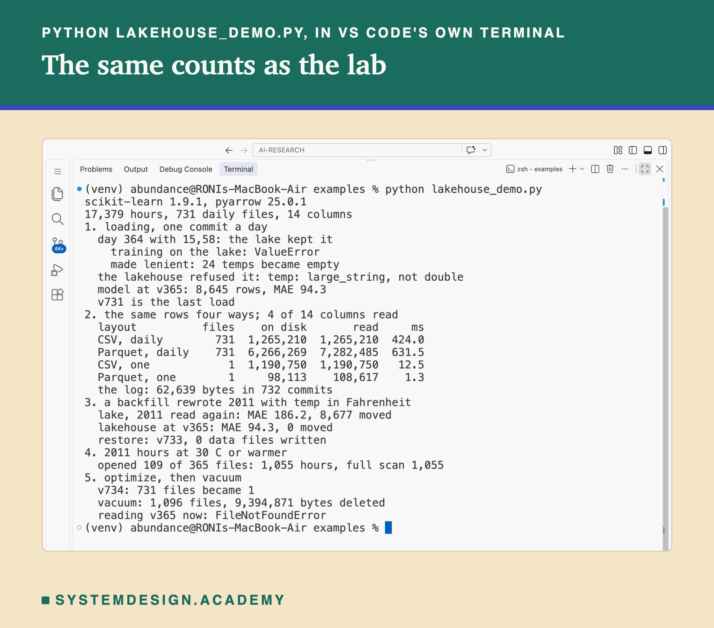
The lake stored it. Writing a CSV file into a folder checks nothing, so there was no error when the file landed. The problem waited for the first reader. When the training job read 2011 from the lake, only that last file's temperatures were text; the other 364 files held numbers. Joined together, the temperature column was a mix of numbers and text. The model then stopped with ValueError: could not convert string to float: '15,58'.

A lenient reader is worse. A common fix for that error is to force the column to numbers and turn anything that fails into an empty value, with pd.to_numeric(errors="coerce"). I tried it. All 24 temperatures of that day became empty, and the trees trained happily, because they accept empty values. No error at all: one day of 2011 now had no temperature, and nothing said so.

The lakehouse refused it. Before committing, the lakehouse compared the file's columns and types with the schema in commit 0. It stopped with temp: large_string, not double. That is pyarrow's name for text, and its name for a number with a decimal point. No file was committed, and the table stayed at version 364. When the day was sent again correctly, it became version 365, and the model learned from that.

This is schema on write and schema on read, measured. The lake is not wrong to accept the file; a landing zone should accept everything. The mistake is to train on the lake directly, where nobody checks the shape. The lakehouse did the checking once, at the door, for every reader after it.

After all 731 daily files had landed, both stores held the same 17,379 rows. I added two more copies, each a single file: the whole table as one CSV file, and as one Parquet file. Then I asked two questions of each. How many bytes does it take on disk? And how many bytes does a reader actually take from the files, to get the 4 columns the model needs out of 14?

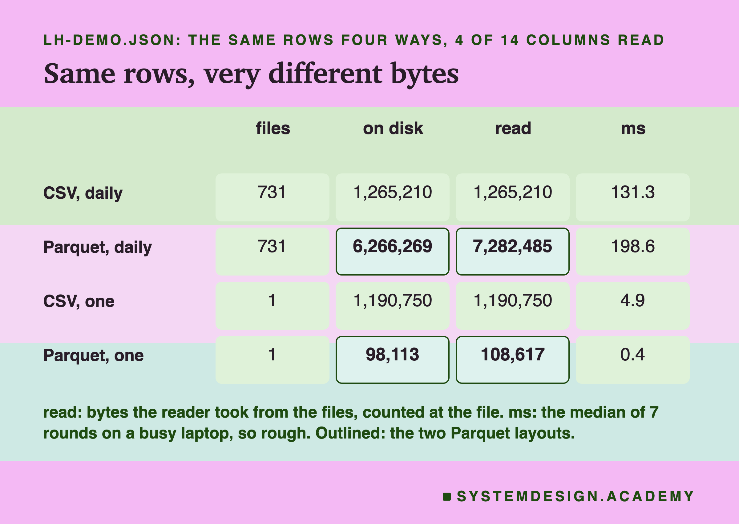
I counted the bytes read with a small wrapper around each file that adds up every byte a reader takes from it. The times are in milliseconds, thousandths of a second. Each is the median of 7 rounds, with the order of the four layouts rotated each round, so each came first at least once. They are rough, because a busy laptop is a noisy clock. The counts of bytes do not move between runs.

CSV has to be read whole. To get 4 columns from a CSV file, a reader must read every line, because the columns are mixed together in each line. So both CSV layouts read every byte they hold: 1,265,210 for the daily files and 1,190,750 for the one file.

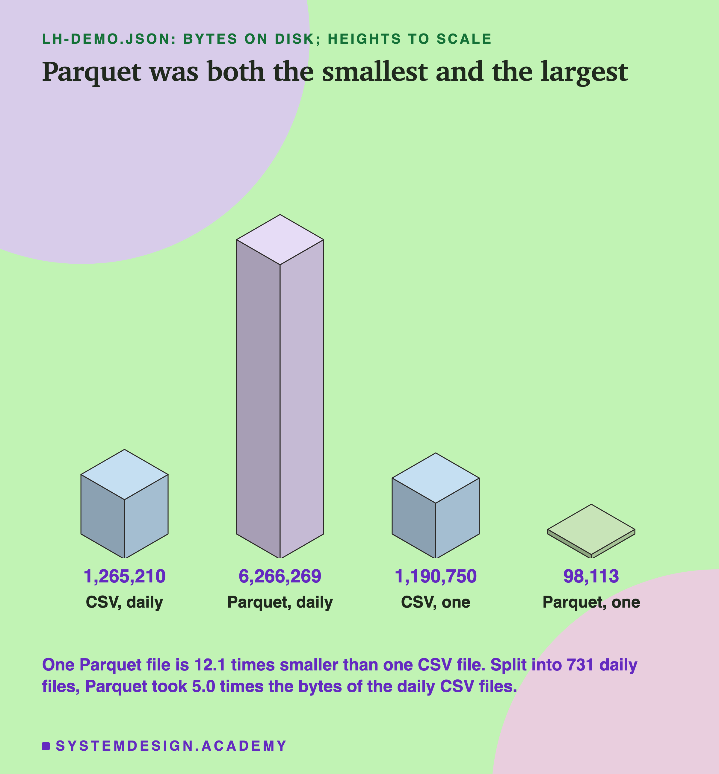
One Parquet file was the smallest by far. It held the whole table in 98,113 bytes, 12.1 times smaller than one CSV file. Parquet stores each column together and compresses it, and a column of hours or temperatures compresses well. Reading it took 0.4 milliseconds, against 4.9 for one CSV file.

731 small Parquet files were the largest by far. The same rows took 6,266,269 bytes, 5.0 times the daily CSV files and 64 times the one Parquet file. They were also the slowest to read, at 198.6 milliseconds. The format that won as one file lost when split into 731 small ones.

The table on the last slide surprised me, so I added two more parts to the report. I wrote them after seeing that table, but before the report itself first ran. They look inside the Parquet files, and log every read the reader makes. Both are in results/lh-report.json.

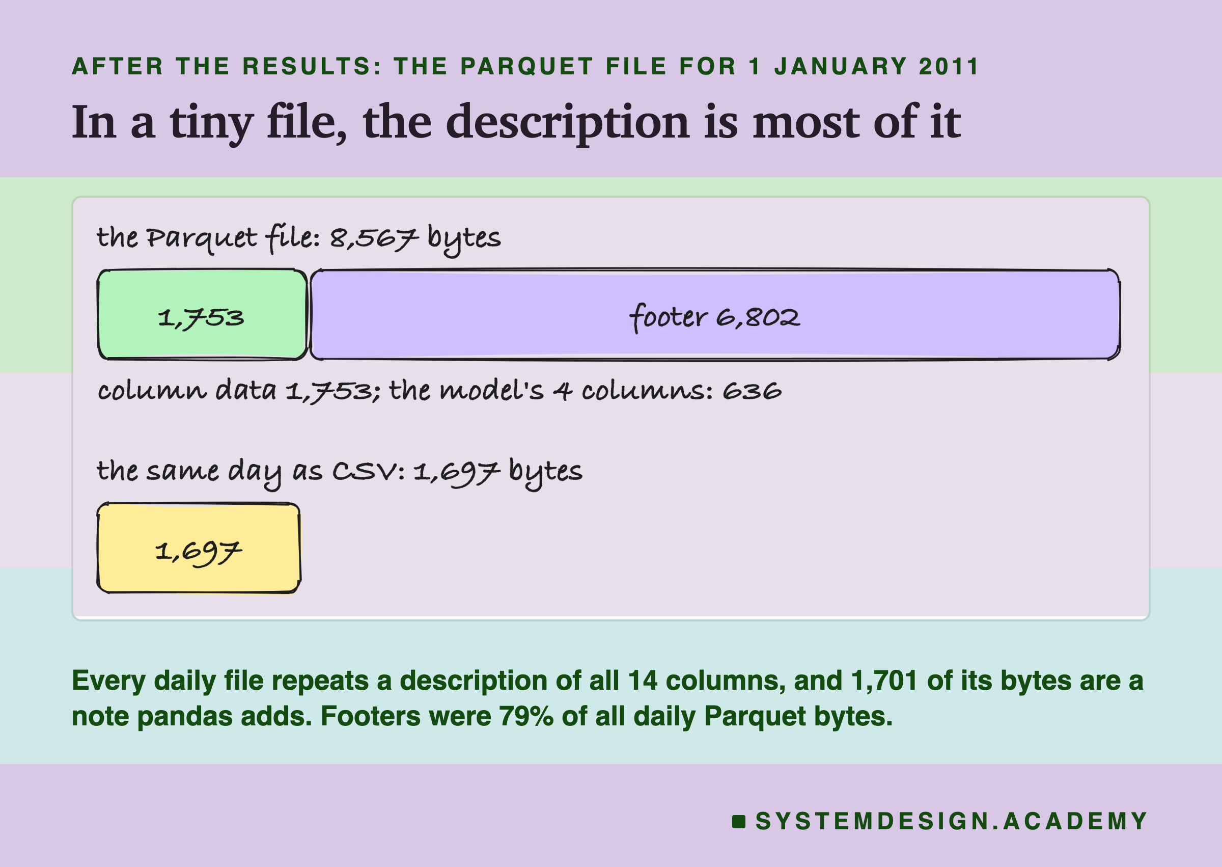
A tiny file is mostly description. The file for 1 January 2011 holds 24 rows in 8,567 bytes. The data itself, all 14 columns, is only 1,753 of them. The footer is 6,802. The other 12 bytes are Parquet's 4-byte markers at each end and the footer's length. The footer describes every column: its name, its type, where it starts, and its lowest and highest value. It also carries a 1,701-byte note that pandas adds so it can rebuild its own table later.

Every one of the 731 daily files repeats all of that, and across them footers were 79% of the bytes. The same day as CSV is 1,697 bytes.

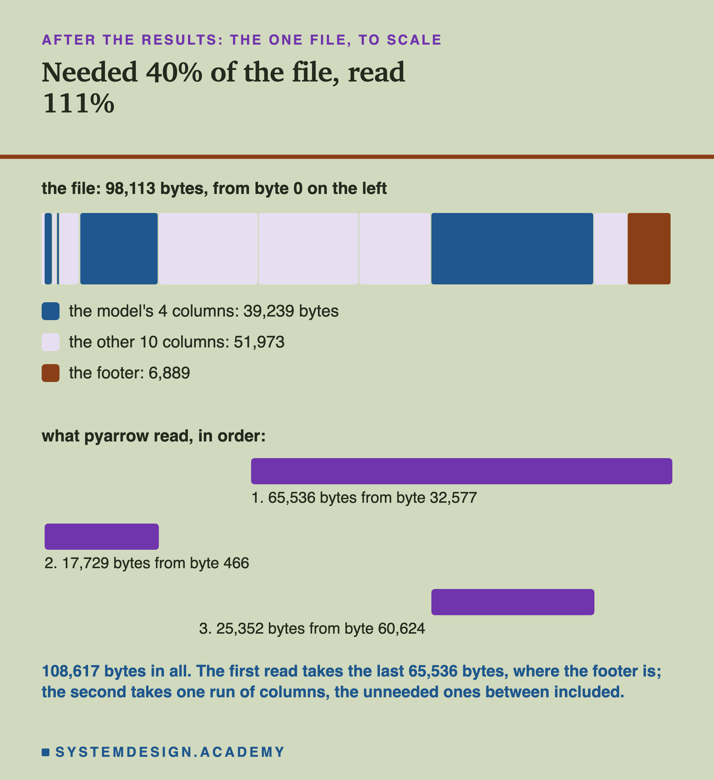
The one file shows why pruning did not save bytes here. In the single file, the model's 4 columns hold 39,239 of the file's 98,113 bytes: 40% of the file, or 43% of its 91,212 bytes of column data. A reader that took exactly those, plus the 6,889-byte footer, would need about 46,000 bytes. pyarrow took 108,617, in three reads. The first took the last 65,536 bytes of the file, where the footer is, in one go. The second took one run of columns from byte 466. That run includes three columns the model does not need, because they sit between ones it does. The third took the column.

The second event is the one the lakehouse is for. After all of 2012 had loaded, a backfill reran the 2011 job with a bug: it wrote every 2011 temperature in Fahrenheit. The rows, hours and rides were all still right, and the temperatures were all wrong.

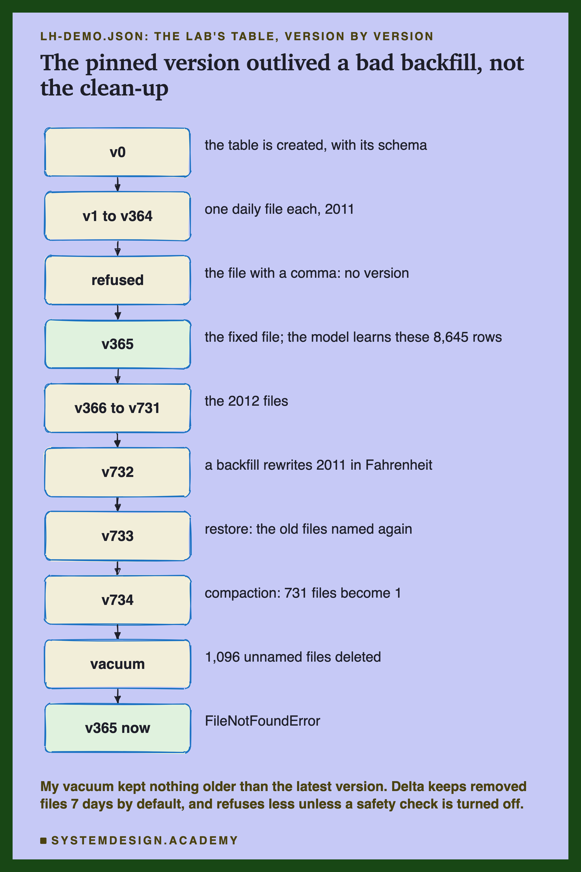
In the lake, the backfill overwrote the 365 CSV files of 2011 in place. In the lakehouse, it wrote 365 new files and one commit, version 732, which removed the old files from the latest version. The old files were still on disk, named by version 365 and earlier.

Then I did what an auditor would ask for. I retrained the same model on 2011 twice: once read from the lake, and once from the lakehouse at the pinned version, 365. Then I compared each model's guesses on the 8,734 test hours with the first model's.

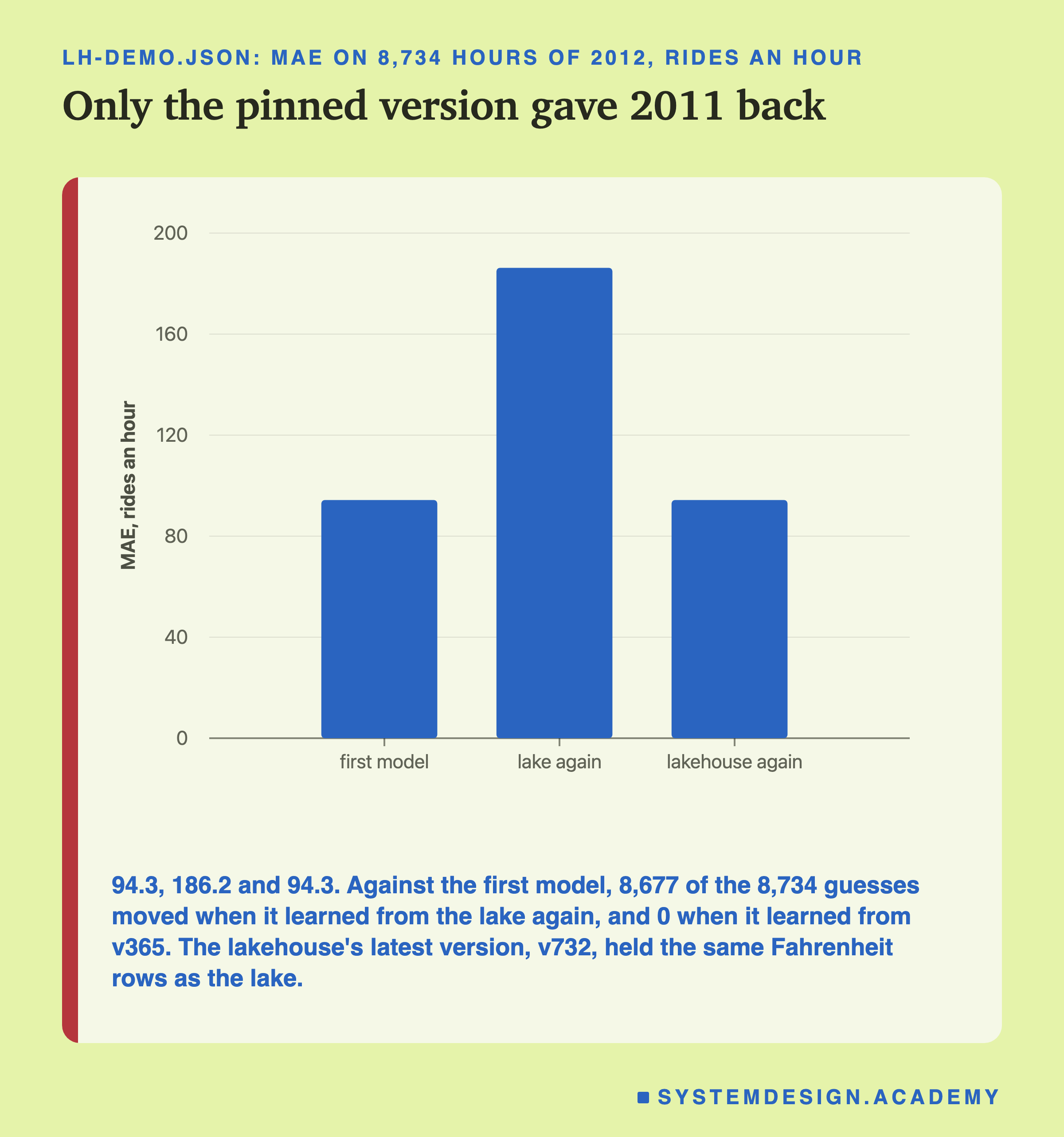
From the pinned version, nothing moved. Version 365 gave back exactly the rows the first model learned from, and the retrained model's guesses matched the first model's on all 8,734 test hours. Its MAE was 94.3, as before. The same rows are only half of that result. The trees were also built with the same code and a fixed seed, random_state=0, and all three together give the same model. Lesson 2 of the lifecycle chapter shows how much a new seed alone can move one.

The third event was a query: every 2011 hour at 30 degrees Celsius or warmer. A plain folder of files must open every 2011 file to answer it. My lakehouse does not, because each commit in my log recorded each file's lowest and highest temperature.

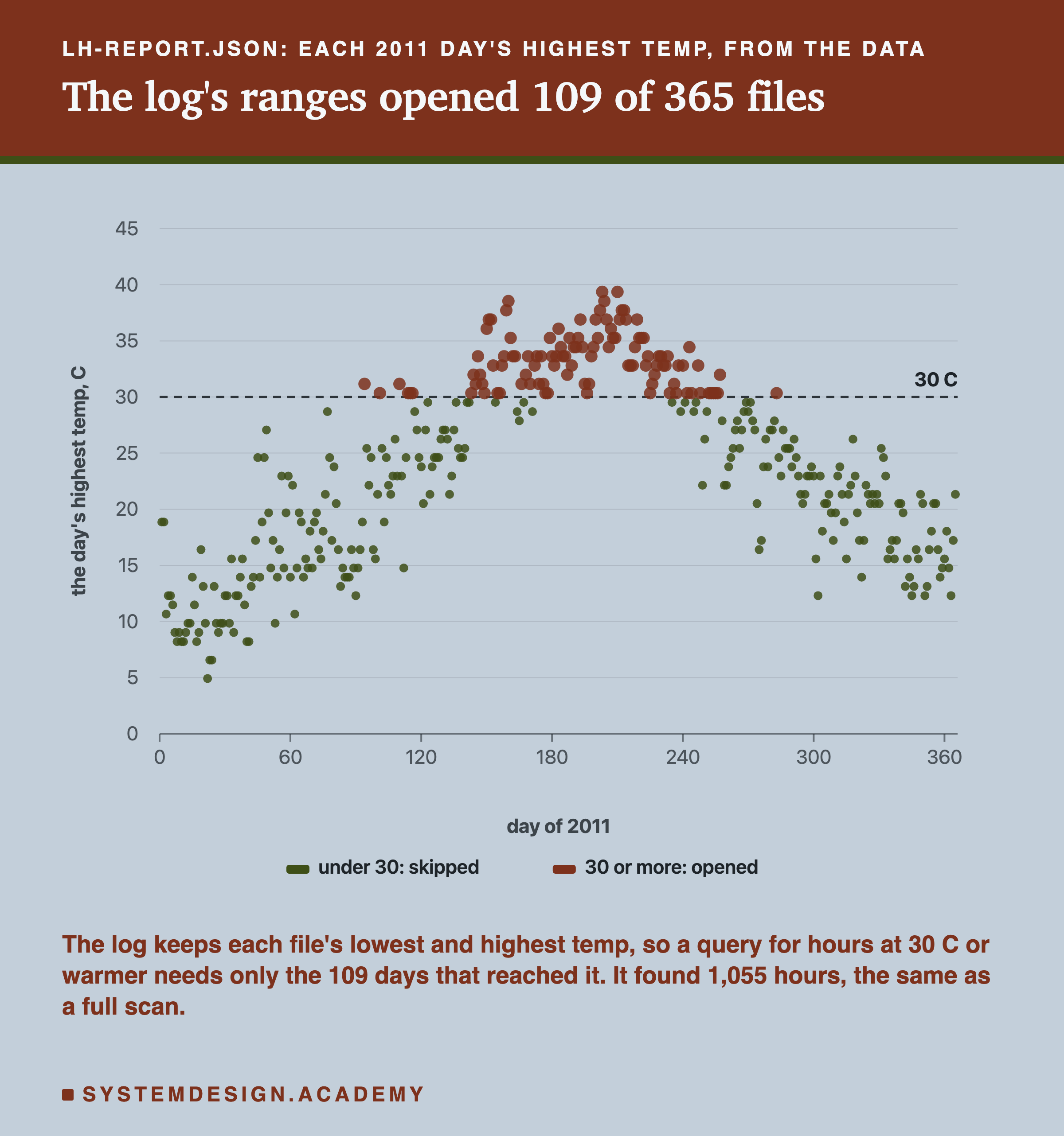
The reader looked only at the log first. Any 2011 file whose highest temperature was under 30 could not hold a match, so it stayed closed. That left 109 of the 365 files, one for each day that reached 30 degrees. Reading just those found 1,055 hours. A full scan of every file found the same 1,055.

This is file skipping, the first trick from the query slide, and it cost almost nothing: a few numbers in each commit. Real formats keep the same kind of numbers. Delta keeps them per file in its log, and Iceberg in its manifests, the files that list a snapshot's data files.

It works best when the files split along the thing you filter on. Here, each file is one day, and a day's temperatures sit close together, so the ranges are narrow. Suppose each file held a random mix of hours from the whole year. Then far more files would have a range that reaches 30, and far fewer could be skipped. I did not measure that case.

The last events were the chores from the SQL slide: compaction and vacuum. Both are good ideas, and the order and the retention decide what they cost you.

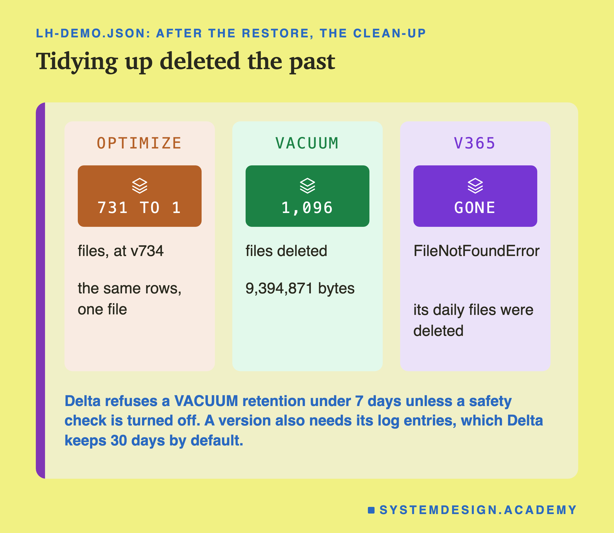
Compaction wrote the live rows as one file and committed version 734, which removed all 731 daily files from the latest version. The report checked that the rows before and after were identical. After it, the latest version needed one file of 98,113 bytes instead of 731 files and 6,266,269 bytes.

Vacuum deleted every file the latest version did not name: the 731 daily files and the 365 Fahrenheit files, 1,096 files and 9,394,871 bytes. Then I asked for version 365 again, the version the model learned from. It failed with FileNotFoundError, because every file it named was gone.

Those bytes are the price of history. The price per terabyte is the same as a lake's, but old versions are extra bytes until you vacuum. Just before vacuum, my lakehouse folder held 9,492,984 bytes of Parquet files, and only 98,113 of them made up the current table. Its log added 144,016 bytes. The lake's CSV folder held 1,273,027 bytes, with no history at all.

I chose the harshest setting on purpose: my vacuum kept nothing older than the latest version. It is not a recipe. Delta refuses a retention under 7 days unless you turn off a safety check. Its documentation warns that with too short a retention, concurrent readers can fail or, "worse, tables can be corrupted".

A real team would choose far longer windows for training tables, for both the data files and the log. But the mechanism is the same at any setting. When either window runs out, the version a model learned from stops existing, and the model can no longer be rebuilt from its data. Choose retention from how long a model must stay explainable, not from how much disk you would like back.

This script is the lab: one file, run from the top. It downloads the same data and builds the lake and the lakehouse in a temporary folder. Then it plays the five events and prints every number on the last few slides. It trains four small models, so it needs no GPU.

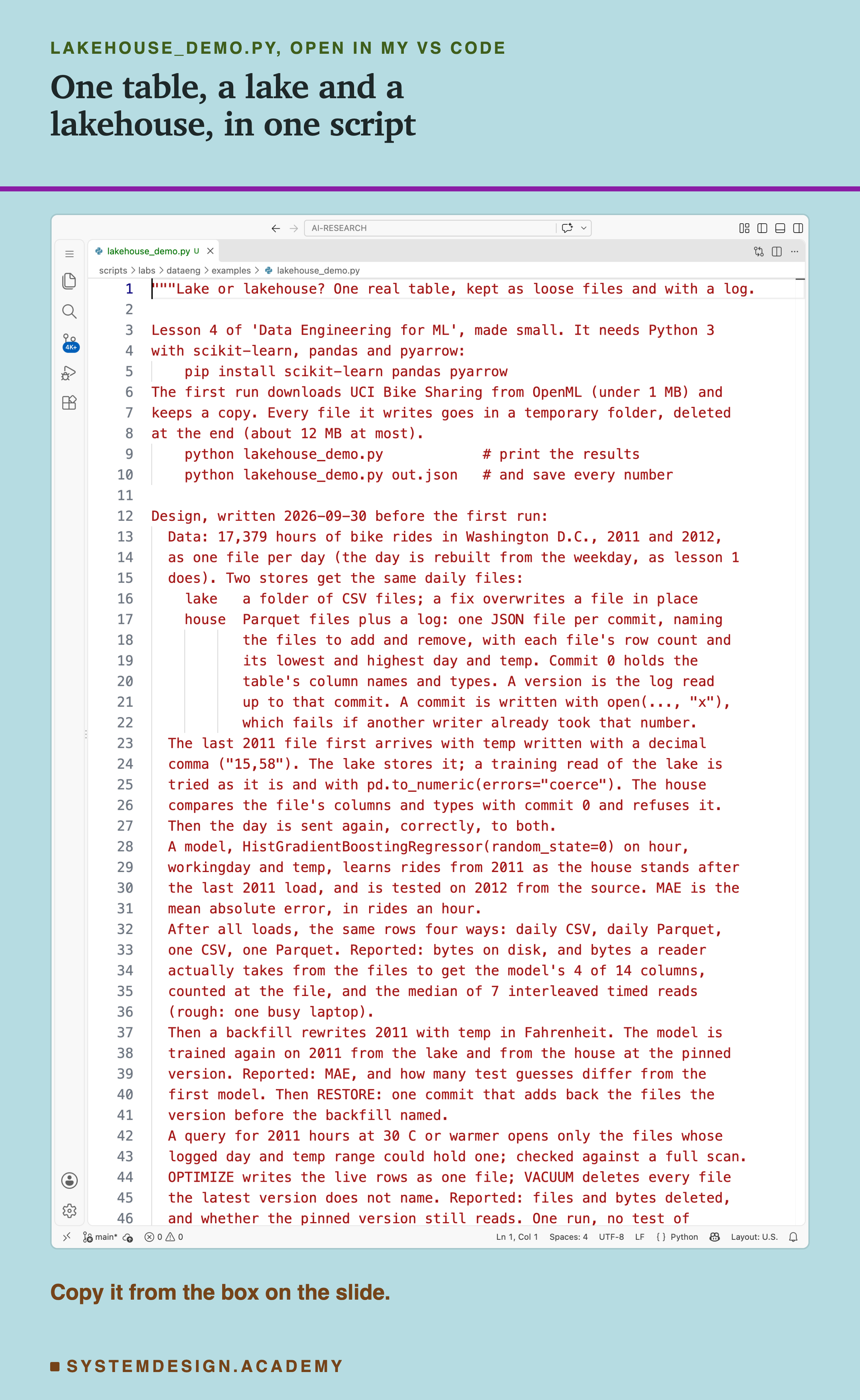
Before you run this lab. You need Python 3 and three libraries: pip install scikit-learn pandas pyarrow. scikit-learn holds the model and the download, and brings NumPy with it. pandas holds the tables, and pyarrow reads and writes Parquet. The first run downloads Bike Sharing from OpenML (under 1 MB compressed), so it needs an internet connection once. scikit-learn keeps a copy in a folder in your home directory (scikit_learn_data) for later runs.

Every file the script writes goes in a temporary folder, about 12 MB at most, and the folder is deleted when the script ends. On my Mac it took 20 to 24 seconds over three runs. I ran it with scikit-learn 1.9.1 and pyarrow 25.0.1. Other versions may give different byte counts, because the Parquet writer changes, so the first line printed is the versions. The libraries run the same way on Windows and Linux, but I have not checked the numbers there.

"""Lake or lakehouse? One real table, kept as loose files and with a log.

Lesson 4 of 'Data Engineering for ML', made small. It needs Python 3
with scikit-learn, pandas and pyarrow:
    pip install scikit-learn pandas pyarrow
The first run downloads UCI Bike Sharing from OpenML (under 1 MB) and
keeps a copy. Every file it writes goes in a temporary folder, deleted
at the end (about 12 MB at most).
    python lakehouse_demo.py            # print the results
    python lakehouse_demo.py out.json   # and save every number

Design, written 2026-09-30 before the first run:
  Data: 17,379 hours of bike rides in Washington D.C., 2011 and 2012,
  as one file per day (the day is rebuilt from the weekday, as lesson 1
  does). Two stores get the same daily files:
    lake   a folder of CSV files; a fix overwrites a file in place
    house  Parquet files plus a log: one JSON file per commit, naming
           the files to add and remove, with each file's row count and
           its lowest and highest day and temp. Commit 0 holds the
           table's column names and types. A version is the log read
           up to that commit. A commit is written with open(..., "x"),
           which fails if another writer already took that number.
  The last 2011 file first arrives with temp written with a decimal
  comma ("15,58"). The lake stores it; a training read of the lake is
  tried as it is and with pd.to_numeric(errors="coerce"). The house
  compares the file's columns and types with commit 0 and refuses it.
  Then the day is sent again, correctly, to both.
  A model, HistGradientBoostingRegressor(random_state=0) on hour,
  workingday and temp, learns rides from 2011 as the house stands after
  the last 2011 load, and is tested on 2012 from the source. MAE is the
  mean absolute error, in rides an hour.
  After all loads, the same rows four ways: daily CSV, daily Parquet,
  one CSV, one Parquet. Reported: bytes on disk, and bytes a reader
  actually takes from the files to get the model's 4 of 14 columns,
  counted at the file, and the median of 7 interleaved timed reads
  (rough: one busy laptop).
  Then a backfill rewrites 2011 with temp in Fahrenheit. The model is
  trained again on 2011 from the lake and from the house at the pinned
  version. Reported: MAE, and how many test guesses differ from the
  first model. Then RESTORE: one commit that adds back the files the
  version before the backfill named.
  A query for 2011 hours at 30 C or warmer opens only the files whose
  logged day and temp range could hold one; checked against a full scan.
  OPTIMIZE writes the live rows as one file; VACUUM deletes every file
  the latest version does not name. Reported: files and bytes deleted,
  and whether the pinned version still reads. One run, no test of
  significance; the timings are rough, the counts and bytes are exact.

Author: Roni Das
Created: 2026-09-30
"""
import atexit
import io
import json
import shutil
import sys
import tempfile
import time
from pathlib import Path

import numpy as np
import pandas as pd
import pyarrow as pa
import pyarrow.parquet as pq
import sklearn
from sklearn.datasets import fetch_openml
from sklearn.ensemble import HistGradientBoostingRegressor

data = fetch_openml("Bike_Sharing_Demand", version=2, as_frame=True,
                    parser="auto").frame
wd = data["weekday"].to_numpy()
day = np.r_[0, np.cumsum((wd[1:] - wd[:-1]) % 7)]  # a new day
table = data.assign(
    day=day, season=data["season"].astype(str),
    holiday=data["holiday"].astype(str) == "True",
    workingday=data["workingday"].astype(str) == "True",
    weather=data["weather"].astype(str))
DAYS = [g for _, g in table.groupby("day")]
FEATS = ["hour", "workingday", "temp"]
COLS = FEATS + ["count"]  # what the model reads
test = table[table["year"] == 1]
out = {"scikit_learn": sklearn.__version__, "pyarrow": pa.__version__,
       "rows": len(table), "files": len(DAYS), "columns": table.shape[1]}
print(f"scikit-learn {sklearn.__version__}, pyarrow {pa.__version__}")
print(f"{len(table):,} hours, {len(DAYS)} daily files, "
      f"{table.shape[1]} columns")

tmp = Path(tempfile.mkdtemp())
atexit.register(shutil.rmtree, tmp)  # delete everything at the end
LAKE, HOUSE = tmp / "lake", tmp / "house"
LOG = HOUSE / "_log"
LOG.mkdir(parents=True)
LAKE.mkdir()


def types(t):
    return {f.name: str(f.type) for f in t.schema}


def commit(actions):
    v = len(list(LOG.iterdir()))
    with open(LOG / f"{v:05d}.json", "x") as f:  # "x": v not taken
        json.dump(actions, f)
    return v


def live(v):
    files = {}
    for k in range(v + 1):
        c = json.loads((LOG / f"{k:05d}.json").read_text())
        files.update(c.get("add", {}))
        for name in c.get("remove", []):
            del files[name]
    return files  # file name -> its row count and ranges


def read(v, cols=COLS):
    return pd.concat([pd.read_parquet(HOUSE / n, columns=cols)
                      for n in sorted(live(v))], ignore_index=True)


def put(df, name):
    t = pa.Table.from_pandas(df, preserve_index=False)
    want = json.loads((LOG / "00000.json").read_text())["schema"]
    bad = [c for c in want if types(t).get(c) != want[c]]
    if bad:
        raise TypeError(f"{bad[0]}: {types(t)[bad[0]]}, not "
                        f"{want[bad[0]]}")
    pq.write_table(t, HOUSE / name)
    return {name: {"rows": len(df),
                   "day": [int(df["day"].min()), int(df["day"].max())],
                   "temp": [float(df["temp"].min()),
                            float(df["temp"].max())]}}


def fit(train):
    model = HistGradientBoostingRegressor(random_state=0)
    model.fit(train[FEATS], train["count"])
    guess = model.predict(test[FEATS])
    return guess, float(np.abs(guess - test["count"]).mean())


def lake_read(cols=COLS, days=None):
    names = sorted(LAKE.iterdir())[:days]
    return pd.concat([pd.read_csv(p, usecols=cols) for p in names],
                     ignore_index=True)


print("1. loading, one commit a day")
first = pa.Table.from_pandas(DAYS[0], preserve_index=False)
commit({"schema": types(first)})
n2011 = int((table.groupby("day")["year"].first() == 0).sum())
for g in DAYS[:n2011 - 1]:
    g.to_csv(LAKE / f"{g['day'].iloc[0]:03d}.csv", index=False)
    commit({"add": put(g, f"{g['day'].iloc[0]:03d}-a.parquet")})
last = DAYS[n2011 - 1]
name = f"{last['day'].iloc[0]:03d}"
comma = last.assign(temp=last["temp"].map(lambda x: f"{x}".replace(
    ".", ",")))
comma.to_csv(LAKE / f"{name}.csv", index=False)  # the lake keeps it
print(f"  day {name} with {comma['temp'].iloc[0]}: the lake kept it")
try:
    fit(lake_read())
    out["strict"] = "trained"
except ValueError as e:
    out["strict"] = type(e).__name__
print(f"    training on the lake: {out['strict']}")
soft = lake_read().assign(temp=lambda d: pd.to_numeric(
    d["temp"], errors="coerce"))
out["emptied"] = int(soft["temp"].isna().sum())
fit(soft)  # no error: the trees accept empty values
print(f"    made lenient: {out['emptied']} temps became empty")
try:
    put(comma, f"{name}-a.parquet")
except TypeError as e:
    out["refused"] = str(e)
print(f"  the lakehouse refused it: {out['refused']}")
last.to_csv(LAKE / f"{name}.csv", index=False)  # sent again, right
PIN = commit({"add": put(last, f"{name}-a.parquet")})
train = read(PIN)
guess, out["mae"] = fit(train)
print(f"  model at v{PIN}: {len(train):,} rows, MAE {out['mae']:.1f}")
for g in DAYS[n2011:]:
    g.to_csv(LAKE / f"{g['day'].iloc[0]:03d}.csv", index=False)
    LAST = commit({"add": put(g, f"{g['day'].iloc[0]:03d}-a.parquet")})
print(f"  v{LAST} is the last load")
out.update(pin=PIN, pin_rows=len(train), last_load=LAST)

print(f"2. the same rows four ways; {len(COLS)} of "
      f"{table.shape[1]} columns read")
table.to_csv(tmp / "one.csv", index=False)
pq.write_table(pa.Table.from_pandas(table, preserve_index=False),
               tmp / "one.parquet")
LAYOUT = {"CSV, daily": sorted(LAKE.iterdir()),
          "Parquet, daily": [HOUSE / n for n in sorted(live(LAST))],
          "CSV, one": [tmp / "one.csv"],
          "Parquet, one": [tmp / "one.parquet"]}


class Counted(io.FileIO):
    """A file that counts every byte a reader takes from it."""
    got = 0

    def read(self, size=-1):
        b = super().read(size)
        Counted.got += len(b)
        return b

    def readinto(self, buf):
        k = super().readinto(buf)
        Counted.got += k or 0
        return k


def take(paths, count=False):
    for p in paths:
        src = Counted(p) if count else p
        if p.suffix == ".csv":
            pd.read_csv(src, usecols=COLS)
        else:
            pq.read_table(src, columns=COLS)
        if count:
            src.close()


ms = {k: [] for k in LAYOUT}
for r in range(7):  # 7 rounds; the order rotates, 4 orders in all
    for k in list(LAYOUT)[r % 4:] + list(LAYOUT)[:r % 4]:
        t0 = time.perf_counter()
        take(LAYOUT[k])
        ms[k].append(1000 * (time.perf_counter() - t0))
out["layouts"] = {}
print(f"  {'layout':<15}{'files':>6}{'on disk':>11}{'read':>11}"
      f"{'ms':>7}")
for k, paths in LAYOUT.items():
    Counted.got = 0
    take(paths, count=True)
    size = sum(p.stat().st_size for p in paths)
    out["layouts"][k] = {"files": len(paths), "bytes": size,
                         "read": Counted.got, "ms": ms[k]}
    print(f"  {k:<15}{len(paths):>6}{size:>11,}{Counted.got:>11,}"
          f"{np.median(ms[k]):>7.1f}")
out["log_bytes"] = sum(p.stat().st_size for p in LOG.iterdir())
print(f"  the log: {out['log_bytes']:,} bytes in {LAST + 1} commits")

print("3. a backfill rewrote 2011 with temp in Fahrenheit")
old = [f"{g['day'].iloc[0]:03d}-a.parquet" for g in DAYS[:n2011]]
new = {}
for g in DAYS[:n2011]:
    f = g.assign(temp=g["temp"] * 9 / 5 + 32)
    f.to_csv(LAKE / f"{g['day'].iloc[0]:03d}.csv", index=False)
    new.update(put(f, f"{g['day'].iloc[0]:03d}-b.parquet"))
BAD = commit({"add": new, "remove": old})
g_lake, out["lake_mae"] = fit(lake_read(days=n2011))
out["lake_moved"] = int((g_lake != guess).sum())
again = read(PIN)
g_pin, out["pin_mae"] = fit(again)
out["pin_moved"] = int((g_pin != guess).sum())
out["same_rows"] = bool(again.equals(train))
print(f"  lake, 2011 read again: MAE {out['lake_mae']:.1f}, "
      f"{out['lake_moved']:,} moved")
print(f"  lakehouse at v{PIN}: MAE {out['pin_mae']:.1f}, "
      f"{out['pin_moved']:,} moved")
before = len(list(HOUSE.glob("*.parquet")))
back = live(BAD - 1)
FIX = commit({"add": {n: s for n, s in back.items()
                      if n not in live(BAD)},
              "remove": [n for n in live(BAD) if n not in back]})
out.update(bad=BAD, restore=FIX, files_written=len(
    list(HOUSE.glob("*.parquet"))) - before)
print(f"  restore: v{FIX}, {out['files_written']} data files written")

print("4. 2011 hours at 30 C or warmer")
files = live(FIX)
END = int(DAYS[n2011 - 1]["day"].iloc[0])  # the last 2011 day
hit = [n for n, s in files.items()
       if s["day"][0] <= END and s["temp"][1] >= 30]
rows = pd.concat([pd.read_parquet(HOUSE / n) for n in hit])
rows = rows[(rows["year"] == 0) & (rows["temp"] >= 30)]
full = read(FIX, None)
full = full[(full["year"] == 0) & (full["temp"] >= 30)]
out["skip"] = {"opened": len(hit), "of": n2011, "hours": len(rows),
               "same": len(rows) == len(full)}
print(f"  opened {len(hit)} of {n2011} files: {len(rows):,} hours, "
      f"full scan {len(full):,}")

print("5. optimize, then vacuum")
OPT = commit({"add": put(read(FIX, None), "all-c.parquet"),
              "remove": list(live(FIX))})
keep = live(OPT)
gone = [p for p in HOUSE.glob("*.parquet") if p.name not in keep]
out["vacuum"] = {"files": len(gone),
                 "bytes": sum(p.stat().st_size for p in gone)}
for p in gone:
    p.unlink()
print(f"  v{OPT}: {len(files)} files became 1")
print(f"  vacuum: {len(gone):,} files, "
      f"{out['vacuum']['bytes']:,} bytes deleted")
try:
    read(PIN)
    out["pin_after_vacuum"] = "read"
except FileNotFoundError as e:
    out["pin_after_vacuum"] = type(e).__name__
print(f"  reading v{PIN} now: {out['pin_after_vacuum']}")
out["optimize"] = OPT

if len(sys.argv) > 1:  # a file name was given: save every number too
    json.dump(out, open(sys.argv[1], "w"), indent=1)

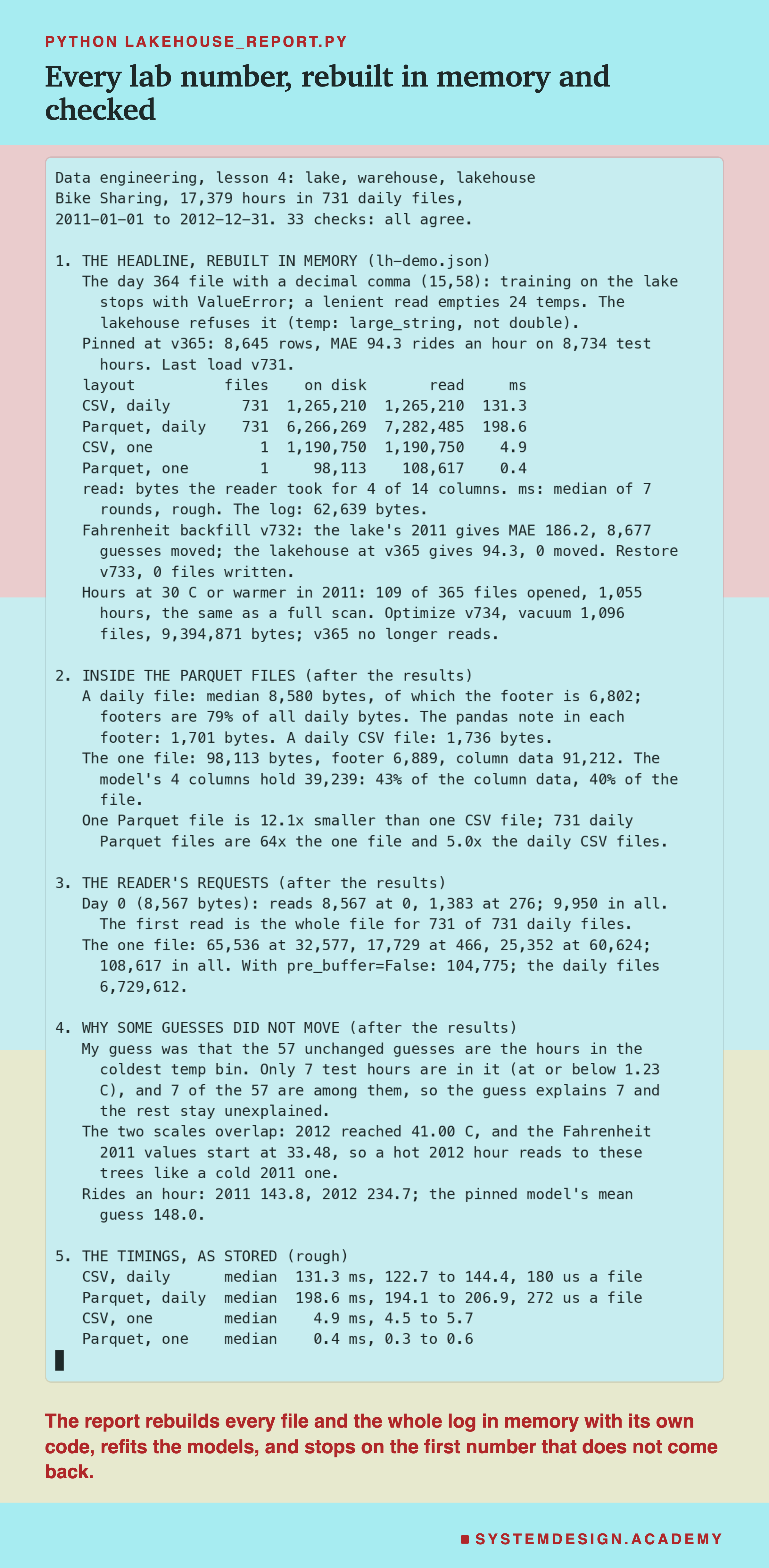
The report lives in scripts/labs/dataeng/lakehouse_report.py. It reads the demo's stored results and the Bike Sharing data from scikit-learn's local copy. It does not trust the demo's code. With its own, separately written code, it rebuilds every daily file, both single files and the whole log, all in memory, without writing a file. It counts the bytes a reader takes over those in-memory copies, and refits the models. It also checks the rebuilt calendar against every row's year, month and weekday. It stops on the first number that does not come back exactly, and all 33 checks agree. The times are not checked, because they move between runs.

Its json mode writes the numbers the figures read to . The mode checks the student script's stored run, line by line. The mode writes the playground on the next slide and checks it against the lab.

This box has no model and no Parquet in it. It holds the real temperature and rides of all 8,645 hours of 2011, one list per day, and the lab's log written in plain Python. A "file" is a list of rows that is never changed after it is written. The log is a list of commits, each naming the files it adds and removes. From those it plays the lab's 2011 story in your browser: the comma file, the pin, the Fahrenheit backfill, the restore, the hot-hours query, compaction and vacuum.

As it is, the box prints the story. The comma file is refused. Version 365 holds 8,645 hours and 1,243,103 rides, with a mean temperature of 20.05 degrees. After the backfill the latest version's mean is 68.09, in Fahrenheit, while version 365 still says 20.05. The restore writes 0 files, and the hot-hours query opens 109 of 365 files and finds 1,055 hours. Vacuum then deletes 730 files, and reading version 365 fails. The report checked each of those against the lab. The box holds 2011 only, so its versions after 365 are smaller than the lab's, and vacuum deletes 730 files, not 1,096.

Then try changing the order of the chores. Move the line GONE = vacuum() above the line OPT = optimize(FIX), and check whether version 365 still reads. Before you run it, decide what you expect, and why. Next, read live(PIN) and live(BAD) and count the files each names. Then try summary(BAD - 1), the version just before the backfill. Last, change the 30 in the hot-hours query to 35, and see how many files it opens.

Loading. fetch_openml("Bike_Sharing_Demand", version=2) downloads the data once, and reads the local copy after that. The day is rebuilt from the weekday: a new day starts wherever the weekday changes. A few columns are turned from categories into plain text or true and false, so that every file has the same simple types. DAYS holds one table per day, and test is 2012, taken straight from the source.

The two stores. LAKE is a folder of CSV files. HOUSE is a folder of Parquet files with a _log folder inside it.

commit and live. commit writes the next numbered JSON file with open(..., "x"). The "x" means create only: if another writer already took that number, it fails instead of overwriting. live(v) replays commits 0 to v, adding and removing file names, and returns the files that make up version v, each with its stats.

put. This is the schema check. It turns a day's table into an Arrow table, compares each column's type with the schema in commit 0, and refuses the file on the first mismatch. Only then does it write the Parquet file. It returns the file's name with its row count and its day and temperature ranges, ready for the next commit.

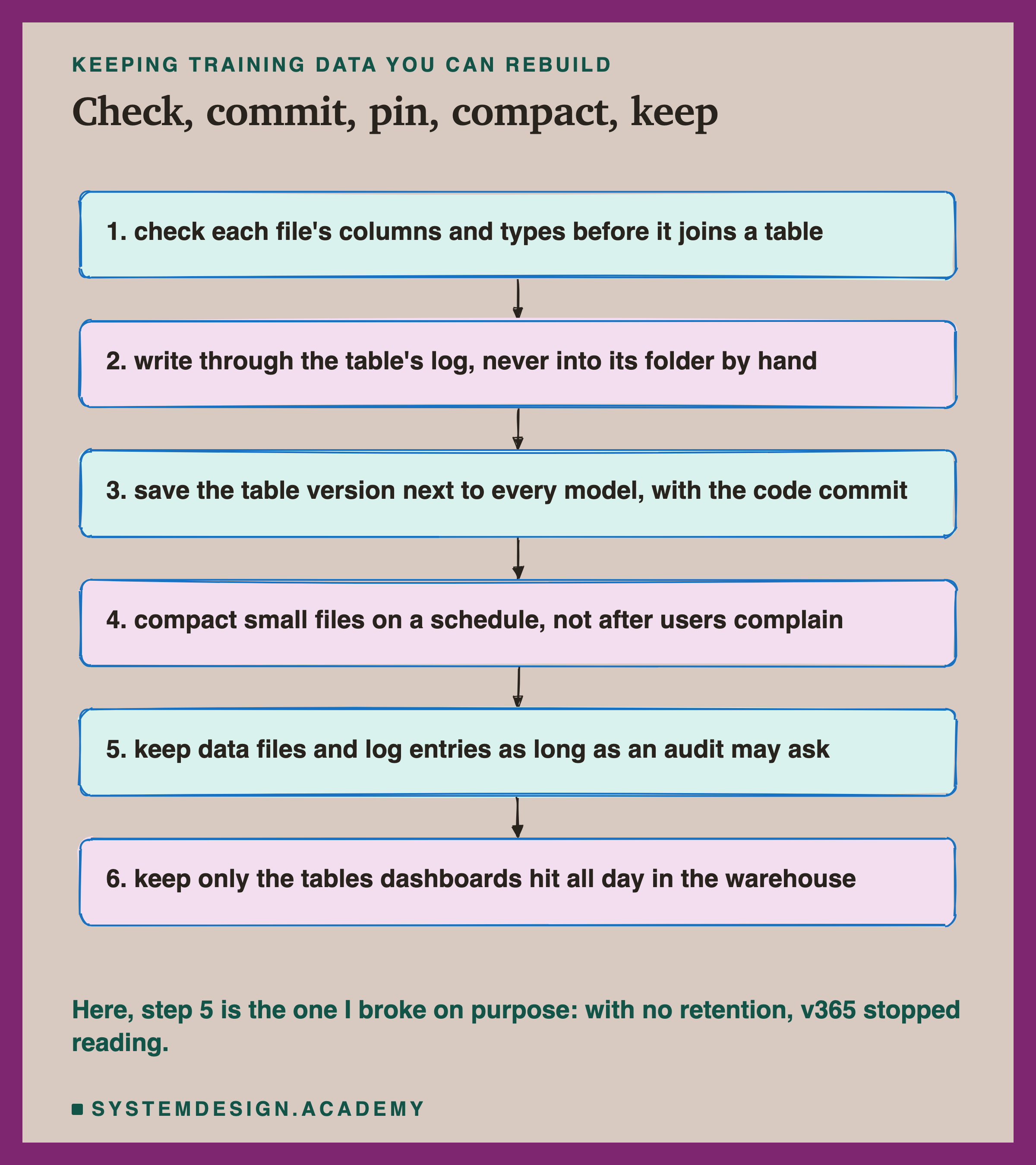
Check each file before it joins a table. Compare its columns and types with the table's schema, and refuse it on a mismatch. Land the raw file anyway, in bronze, so nothing is lost. In the lab, this check stopped the comma file that the lake stored.

Write through the log. Every change goes through the table format's API or SQL, never by copying or deleting files in the folder. A file the log does not name is invisible, and a file the log names but is gone breaks every read of that version.

Pin the version. Save the table version next to every model, in the same record as the code commit and the settings. In the lab, version 365 gave back the same 8,645 rows after a bad backfill, but only because I knew to ask for 365.

Compact on a schedule. Many small files cost bytes and time. Here, 731 daily files took 64 times the bytes of one file. Compaction is a normal job, like a backup.

Keep both windows long enough. Set delta.deletedFileRetentionDuration and delta.logRetentionDuration from how long a model must stay explainable. Both must cover it, because a version needs its data files and its log entries. For a longer audit, copy the training version into its own table with a deep clone or a plain copy, not a shallow clone. In the lab, a vacuum that kept nothing old made the pinned version unreadable.

Keep the warehouse for what needs it. The tables dashboards hit all day belong there. Training tables belong where training code can read their files, at a version.

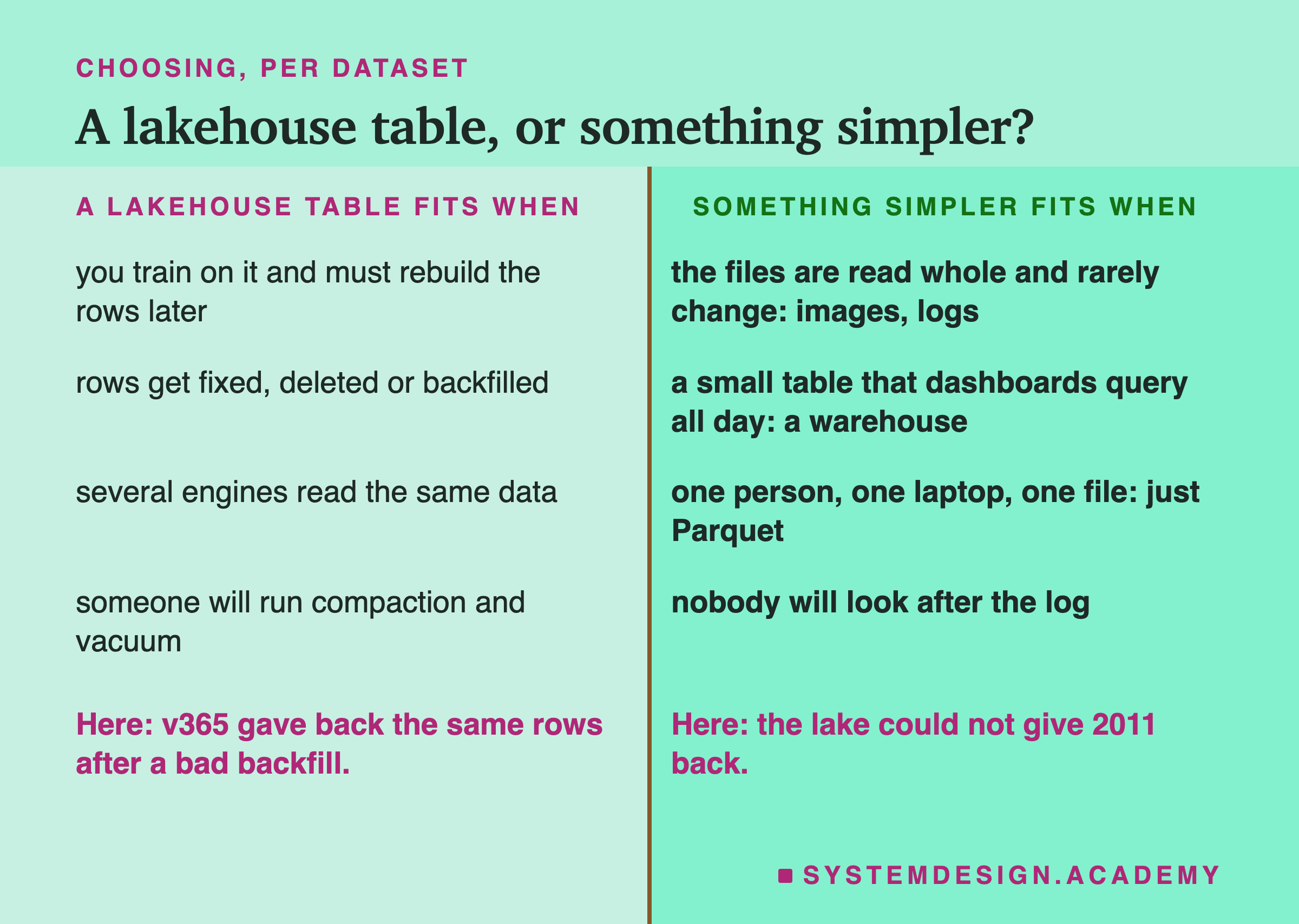
Use a lakehouse table when you train on it and must rebuild the rows later. A version you can read again is the only way to answer "what did this model learn from?" months later.

Use one when rows get fixed, deleted or backfilled. Every change is a new version, and the old one stays readable until you choose to let it go.

Use one when several engines read the same data. A Spark job, an analyst's SQL and a Python script can all read the same files, with one set of checks.

Do not use one when the files are read whole and rarely change, like images or log files. A plain lake is simpler, and a version per image adds nothing.

Do not use one for a small table that dashboards query all day. A warehouse is built for exactly that.

Do not use one if nobody will look after the log. Without compaction the files pile up, and without a chosen retention the history either grows without end or vanishes too early. And for one person working on one laptop, one Parquet file may be all you need.

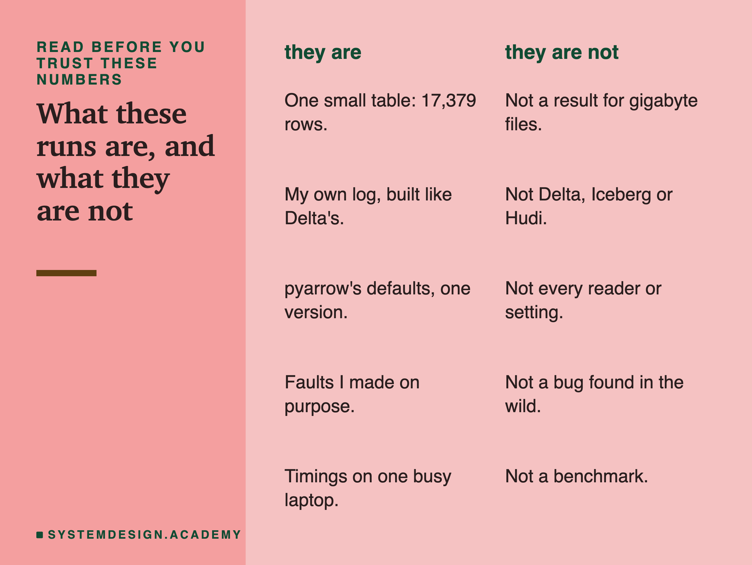
One small table. The whole table is under 1.2 MB as CSV. The byte counts are exact for it, but a table a thousand times larger would behave differently. Above all, reading only some columns saves far more on large files. The small-file cost, though, grows with the number of files, not their size.

My own log, not Delta. The lakehouse here is about 30 lines of Python that follow Delta's idea: numbered JSON commits over Parquet files. It has no checkpoints, no conflict checks between writers, and no real retention window. Real formats behave as their documentation says, and the first half of the lesson quotes it.

One reader, one version. The bytes read come from pyarrow 25.0.1 with its default settings. With pre_buffer=False the single file took 104,775 bytes instead of 108,617. Other readers make other choices.

Faults I made on purpose. The comma file, the Fahrenheit backfill and the vacuum with no retention are simulations of things that happen, not bugs I found in someone's system.

Rough timings. The milliseconds come from one busy laptop, 7 rounds each. They show that 731 files cost far more time than 1, not how much time on any other machine.

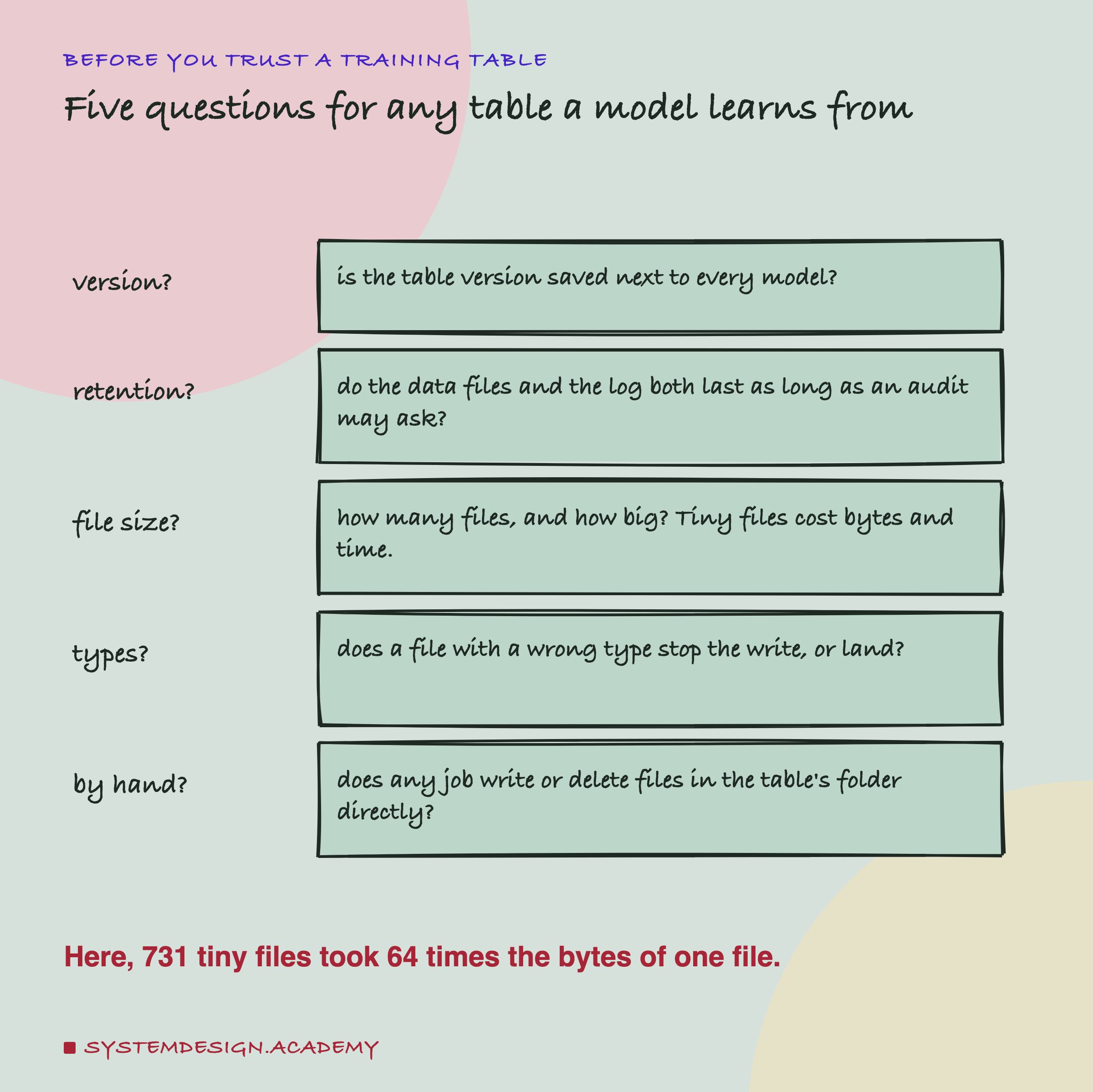
Take one table your team trains on and ask the five questions on the card. If the answer to "version?" is no, start there. Record the table version next to every model you train from today. It costs one line of code, and it is the difference between rebuilding a model and guessing at it.

Then look at the files themselves. Count how many there are and how big they are. If there are thousands of files of a few kilobytes, schedule compaction. Then find out how long the table keeps removed data files, and how long it keeps its log. Compare both with the longest time anyone may ask you to explain a model.

The next lesson, data validation and quality, picks up where the Fahrenheit backfill left off. A schema check caught the comma, but not the wrong unit. Catching that needs checks on the values themselves.

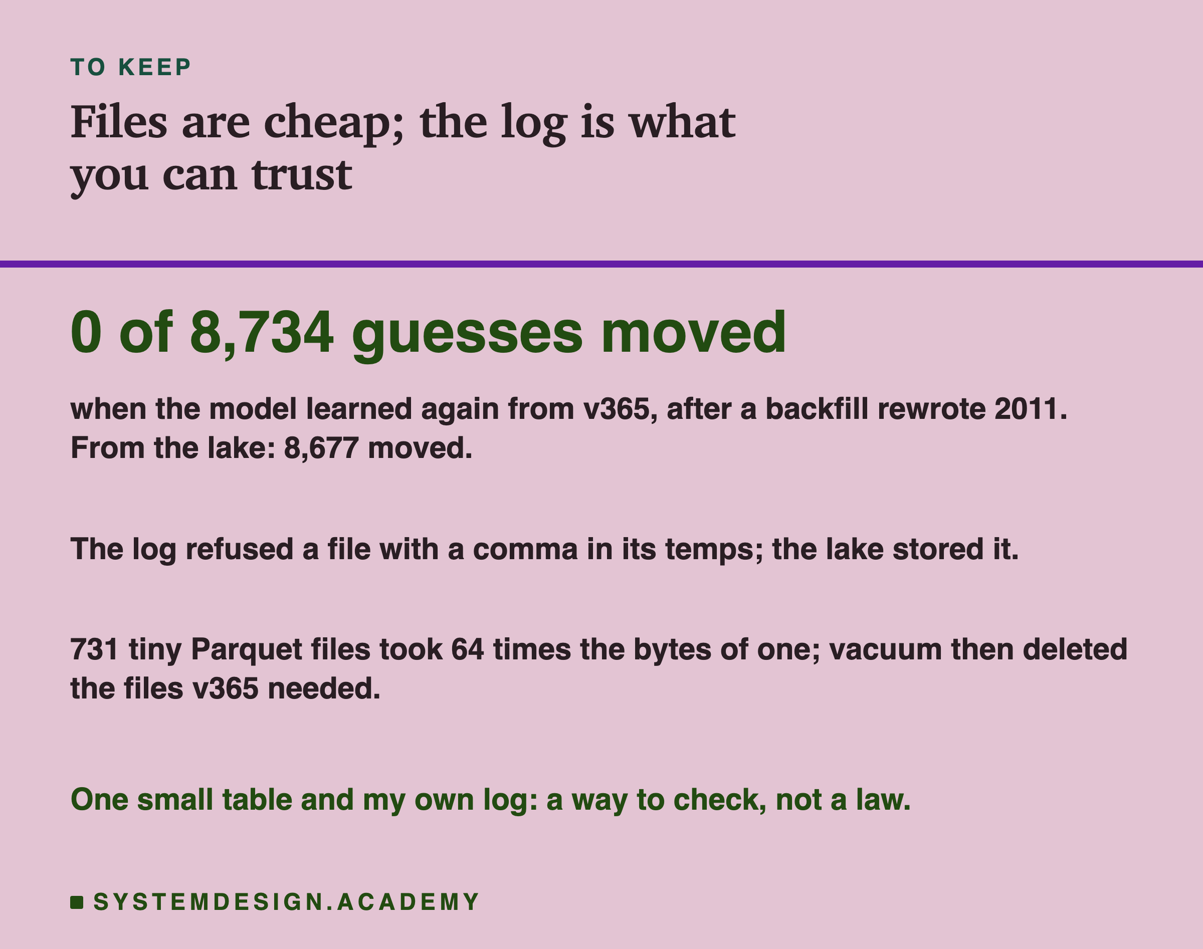
If you keep one thing from this lesson, keep the number at the top of the card. After a backfill rewrote a year of history, the model learned from version 365 again and not one of its 8,734 guesses moved. From the lake, 8,677 moved. The price per terabyte was the same either way, but history was not free: until vacuum ran, my lakehouse kept 9,394,871 bytes of old files. The log made the old rows something you could ask for. Its two retention windows decide how long you can keep asking.