Read this sentence: "The trophy did not fit in the suitcase because it was too big." What was too big? The trophy. Now change one word: "...because it was too small." Now "it" means the suitcase.

You worked that out without effort, by looking back at the earlier words and deciding which one "it" is about. A language model has to do the same kind of thing for every word it reads. The part of the model that does it is called attention.

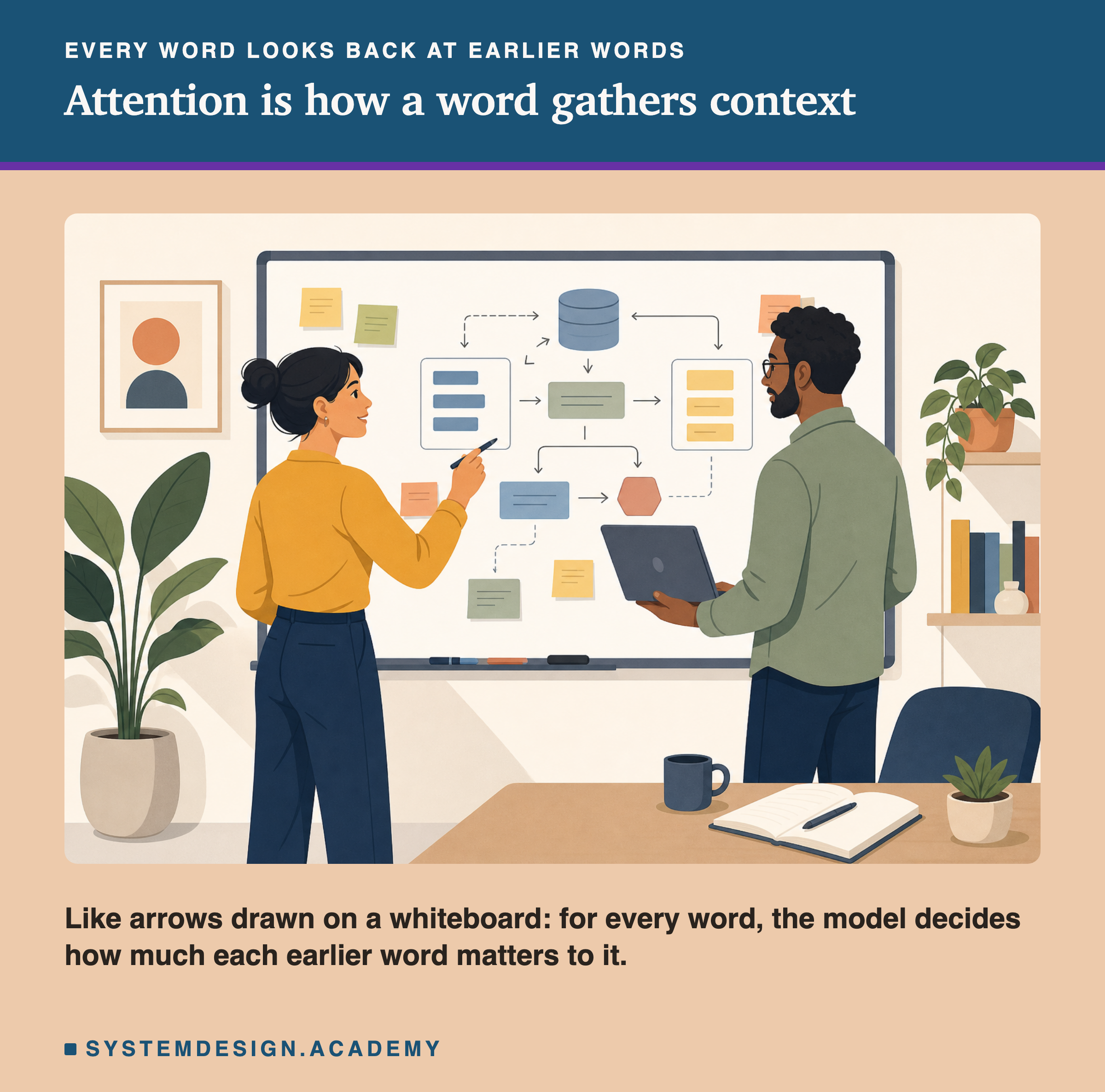
In lesson 3 you saw that the model reads a prompt quickly and writes slowly. This lesson opens up the reading step. You will work out attention by hand with a few small numbers, then read the real attention weights of a real model, and you will find that a real model does not behave exactly like the simple picture.

By the end you will be able to compute attention for one word by hand, read an attention table, explain why a word can only look backwards, and say what attention weights can and cannot tell you.

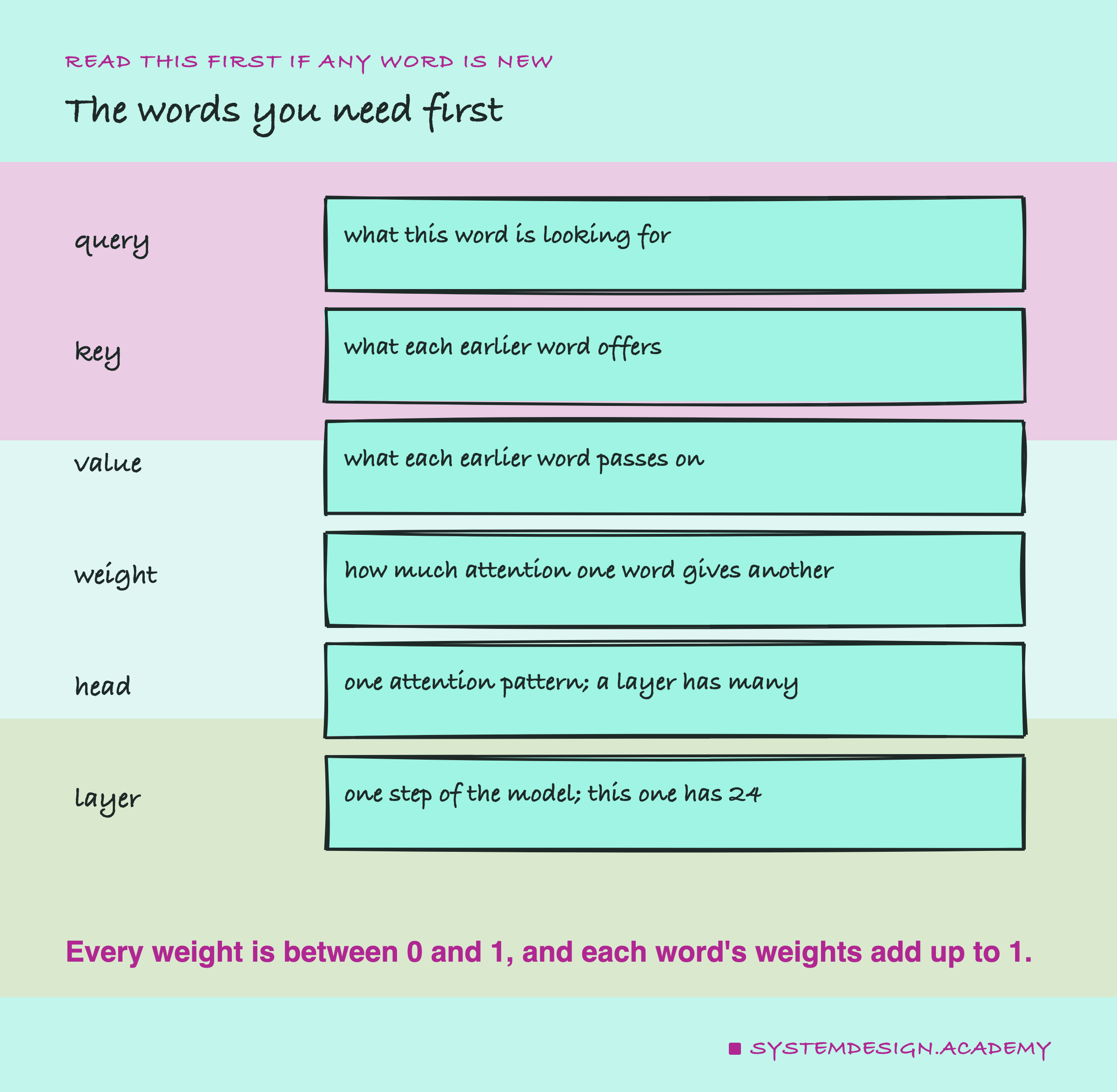
Inside the model, every word (every token, to be exact) is a list of numbers, like the embeddings from the Tokens and Embeddings chapter. Attention works on those lists.

Query. A list of numbers that describes what the current word is looking for. Think of it as a question the word asks.

Key. A list of numbers for each earlier word that describes what it offers. The query is compared with every key.

Value. A list of numbers for each earlier word that holds what it will pass on if it is chosen.

Weight. A number between 0 and 1 that says how much one word pays attention to another. For one word, all its weights add up to exactly 1.

Pronoun and adjective. A pronoun is a short word like "it" or "they" that stands for a noun mentioned elsewhere. An adjective is a describing word like "big" or "small".

Softmax. The step that turns raw scores into weights: it makes every number positive and scales them so they add up to 1. Lesson 1 showed the odds of the next token; softmax is also the step a model uses to make those odds from its scores.

Head. One complete set of queries, keys and values. Each head can learn to look for something different. The model in this lesson has 14 heads in every layer.

Layer. One step of the model. The model here has 24 layers, one after another, and every one of them has attention.

The best way to understand attention is to do it once with small numbers. Real models use hundreds of numbers per word; here each word has only two, and I made them up so the arithmetic is easy to follow.

The sentence is "The cat sat it", and we compute attention for the last word, "it". Its query is [1.0, 0.6]. The keys are: The [0.1, 0.0], cat [1.0, 0.8], sat [0.2, 0.9], it [0.6, 0.5].

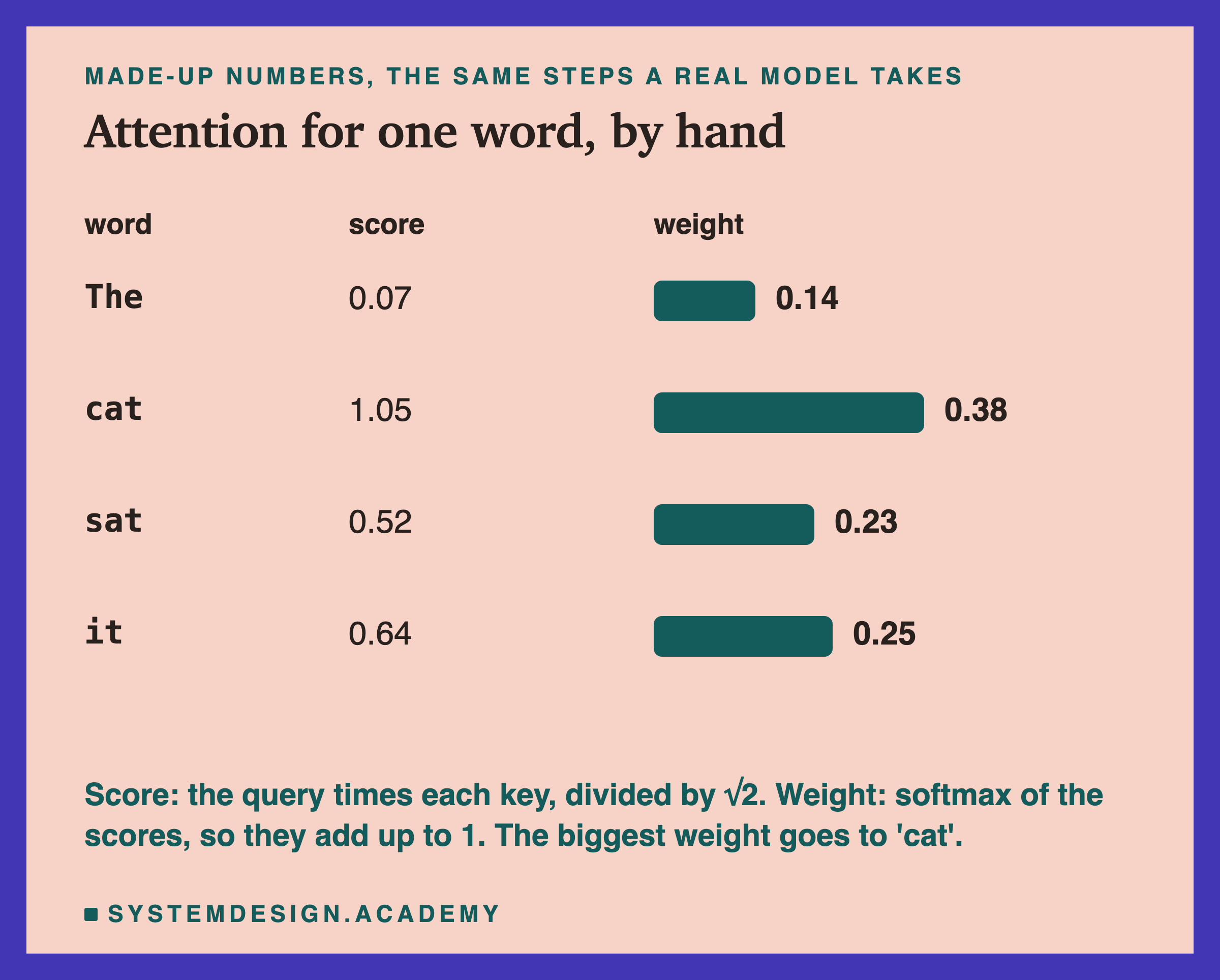
Step 1, a score for each word. Multiply the query and the key number by number, and add. This is the dot product from the Tokens and Embeddings chapter. For "cat": 1.0 × 1.0 + 0.6 × 0.8 = 1.0 + 0.48 = 1.48. Then divide by the square root of the list length, √2 ≈ 1.414: 1.48 ÷ 1.414 ≈ 1.05. The others: "The" is (1.0 × 0.1 + 0.6 × 0.0) ÷ 1.414 ≈ 0.07, "sat" is (0.2 + 0.54) ÷ 1.414 ≈ 0.52, and "it" is (0.6 + 0.3) ÷ 1.414 ≈ 0.64.

The division by √2 keeps the scores from getting too large when the lists are long. Real models divide by the square root of their list length in the same way.

Step 2, softmax. Raise e (about 2.718) to the power of each score: e^0.07 ≈ 1.07, e^1.05 ≈ 2.85, e^0.52 ≈ 1.69, e^0.64 ≈ 1.89. They add up to about 7.50. Divide each by the total: 1.07 ÷ 7.50 ≈ 0.14, 2.85 ÷ 7.50 ≈ 0.38, 1.69 ÷ 7.50 ≈ 0.23, 1.89 ÷ 7.50 ≈ 0.25. These are the weights, and 0.14 + 0.38 + 0.23 + 0.25 = 1.00.

Step 3, blend the values. The output for "it" is each word's value multiplied by its weight, then added up. With the values in the box further down, the result is [0.51, 0.37]. The word "cat" has the largest share, 0.38, but every word contributes something.

That blended list becomes the new meaning of "it" for the next layer. In plain words, "it" has pulled in some of the meaning of "cat".

Step 1 divided every score by √2. That looks like a small detail, but without it attention stops working well in a real model. Here is why, worked with the same numbers.

Without the division. The raw scores are 0.1 for "The", 1.48 for "cat", 0.74 for "sat" and 0.9 for "it". Softmax: e^0.1 ≈ 1.11, e^1.48 ≈ 4.39, e^0.74 ≈ 2.10, e^0.9 ≈ 2.46, which add up to about 10.05. The weights are 1.11 ÷ 10.05 ≈ 0.11, 4.39 ÷ 10.05 ≈ 0.44, 0.21 and 0.24. Compared with the divided version, 0.14, 0.38, 0.23 and 0.25, "cat" now takes more and the others less. Bigger scores make softmax pick a favourite more strongly.

With longer lists. A score is a sum of products, one product per number in the list. The more numbers there are, the bigger the sum tends to get. Qwen2.5-0.5B works with 896 numbers per word, split across its 14 heads, so each head's query and key have 896 ÷ 14 = 64 numbers. To see what bigger scores do, multiply our four divided scores by 8: they become 0.57, 8.37, 4.19 and 5.09. After softmax the weights are about 0.00, 0.95, 0.01 and 0.04. Almost all the weight goes to one word, and the others are nearly ignored.

That is a problem during training. When one weight is almost 1 and the rest almost 0, small changes to the other scores barely change anything, so the model learns slowly. Dividing by the square root of the list size, √64 = 8 for this model, keeps the scores in a range where softmax still spreads some weight around. It is a small, fixed division, and almost every model of this kind uses it.

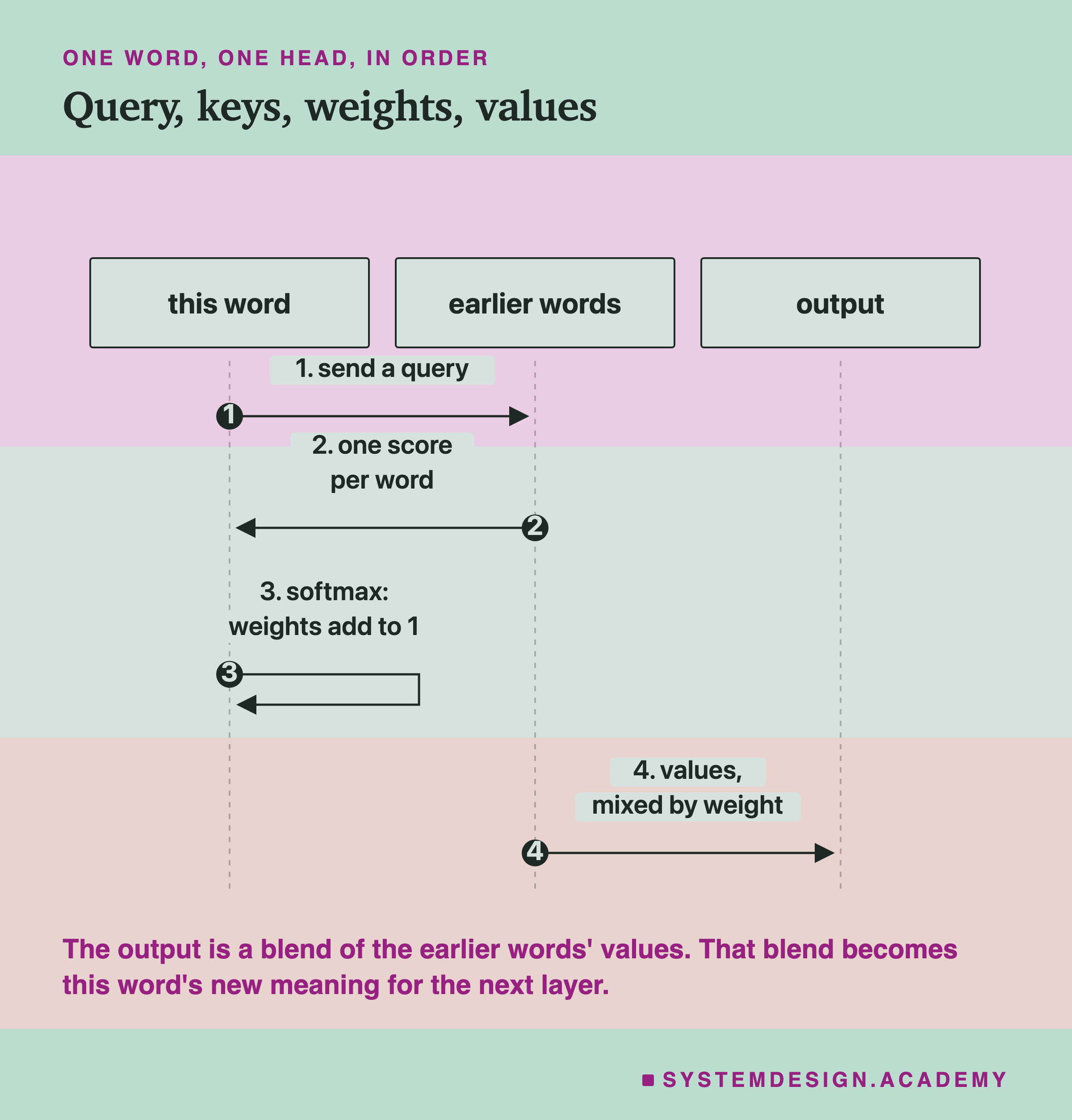
The four steps are the same in every head of every layer: compare the query with each key, turn the scores into weights with softmax, and blend the values using those weights.

Where do the queries, keys and values come from? Each is made from the word's own list of numbers by multiplying it by a table of learned numbers: one kind of table for queries, one for keys and one for values. Those tables are part of the model's weights, learned during training. Nobody writes them by hand. That is general knowledge about how these models are built, not something this lesson measured.

A head that learned tables that happen to link pronouns to nouns will give "it" a large weight on a noun. A head that learned something else will look somewhere else. With 14 heads and 24 layers, this model has 336 different attention patterns for every word.

A single set of queries, keys and values gives one way of looking back. Real models run many of these side by side, and each one is a head.

In Qwen2.5-0.5B, every layer has 14 heads. Each head takes the same words, makes its own queries with its own learned table, and produces its own blended output. The 14 outputs are then joined together into one list per word and passed on. So one layer can look back in 14 different ways at the same time: one head might follow the grammar of the sentence, another might link a word to the one just before it, another might put most of its weight on the first word.

Across 24 layers, that is 24 × 14 = 336 heads. That number matters for this lesson. When the lesson averages "the 14 heads of layer 12", it mixes 14 different patterns into one picture, which can hide what any single head does. When it picks one head out of 336, it can find a pattern that looks meaningful by chance. Both views are useful, and both need care.

One detail about this model: it has 14 query heads but only 2 sets of keys and values, and each set is shared by 7 query heads. So in this model only the queries are truly separate per head. This saves memory when the model writes, and it does not change the four steps you worked by hand.

There is one rule every model in this chapter follows: a word may look at itself and at earlier words, never at later ones.

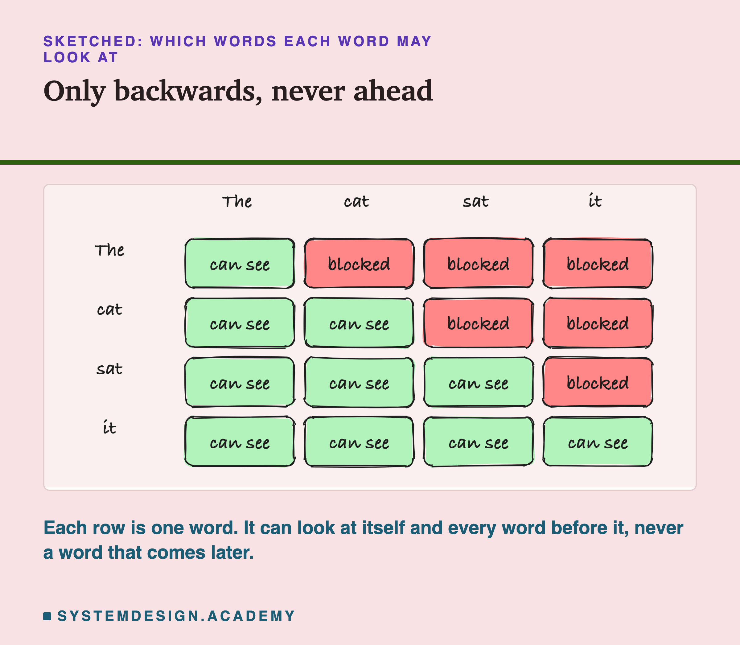
The reason is the writing loop from lesson 3. When the model writes, the later words do not exist yet, so it could never learn to depend on them. To keep reading and writing the same, the model blocks every look ahead, even while reading a prompt where the whole text is already there. In practice the model sets those blocked scores to minus infinity before softmax, so their weights come out as exactly 0.

This has a surprising result for our trophy sentence. When the model reads "it", it has not yet reached "big" or "small". So at the moment of "it", the model cannot know which one "it" means. The decision can only be made by later words, which can look back at both "it" and the adjective. The lab tests this directly.

Now to a real model. Qwen2.5-0.5B is a small model from the same family as the qwen2.5:3b of the earlier lessons. It is small enough to return every attention weight on a laptop.

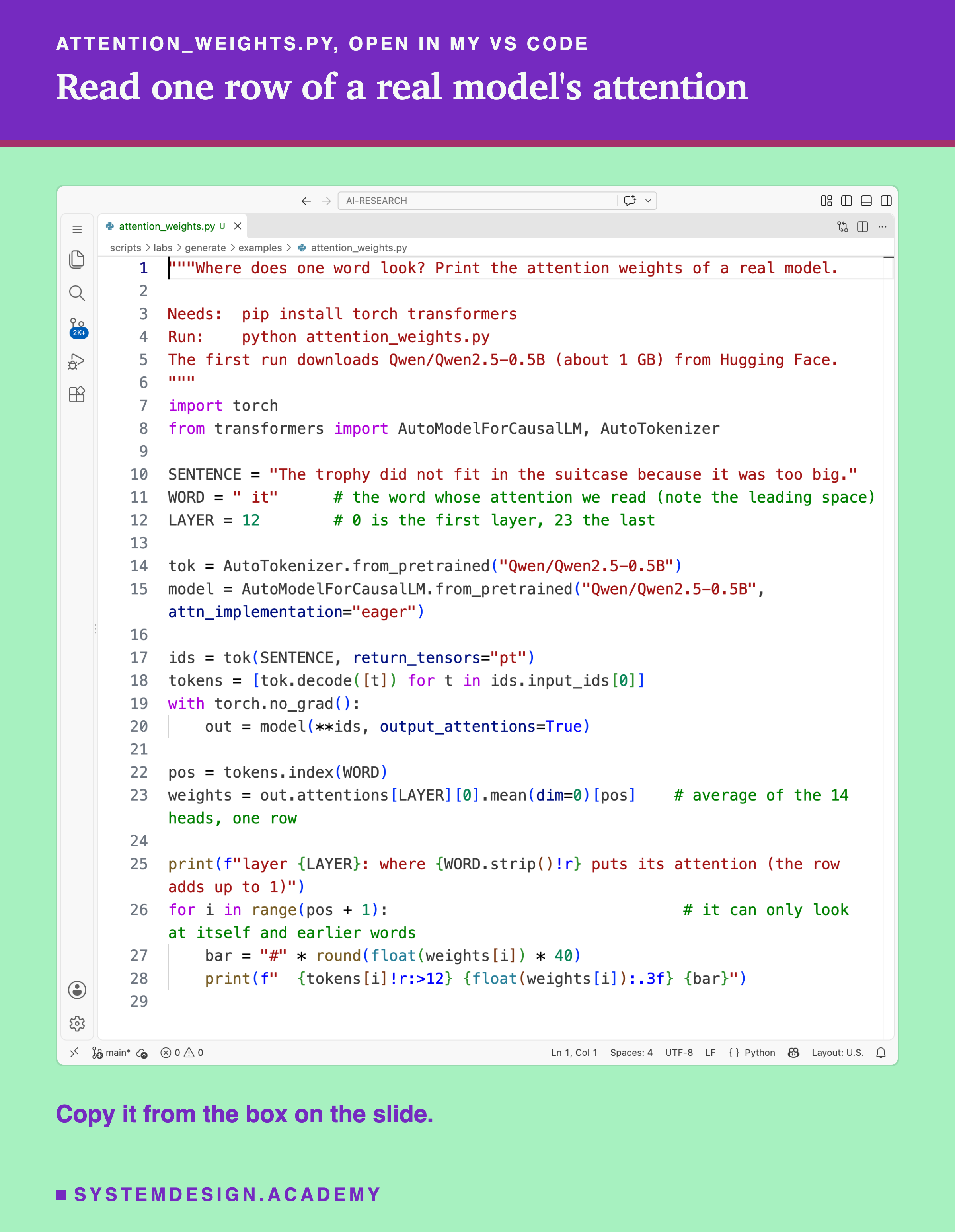
"""Where does one word look? Print the attention weights of a real model.

Needs:  pip install torch transformers
Run:    python attention_weights.py
The first run downloads Qwen/Qwen2.5-0.5B (about 1 GB) from Hugging Face.
"""
import torch
from transformers import AutoModelForCausalLM, AutoTokenizer

SENTENCE = "The trophy did not fit in the suitcase because it was too big."
WORD = " it"      # the word whose attention we read (note the leading space)
LAYER = 12        # 0 is the first layer, 23 the last

tok = AutoTokenizer.from_pretrained("Qwen/Qwen2.5-0.5B")
model = AutoModelForCausalLM.from_pretrained("Qwen/Qwen2.5-0.5B", attn_implementation="eager")

ids = tok(SENTENCE, return_tensors="pt")
tokens = [tok.decode([t]) for t in ids.input_ids[0]]
with torch.no_grad():
    out = model(**ids, output_attentions=True)

pos = tokens.index(WORD)
weights = out.attentions[LAYER][0].mean(dim=0)[pos]    # average of the 14 heads, one row

print(f"layer {LAYER}: where {WORD.strip()!r} puts its attention (the row adds up to 1)")
for i in range(pos + 1):                                # it can only look at itself and earlier words
    bar = "#" * round(float(weights[i]) * 40)
    print(f"  {tokens[i]!r:>12} {float(weights[i]):.3f} {bar}")

This is what it printed in VS Code's terminal.

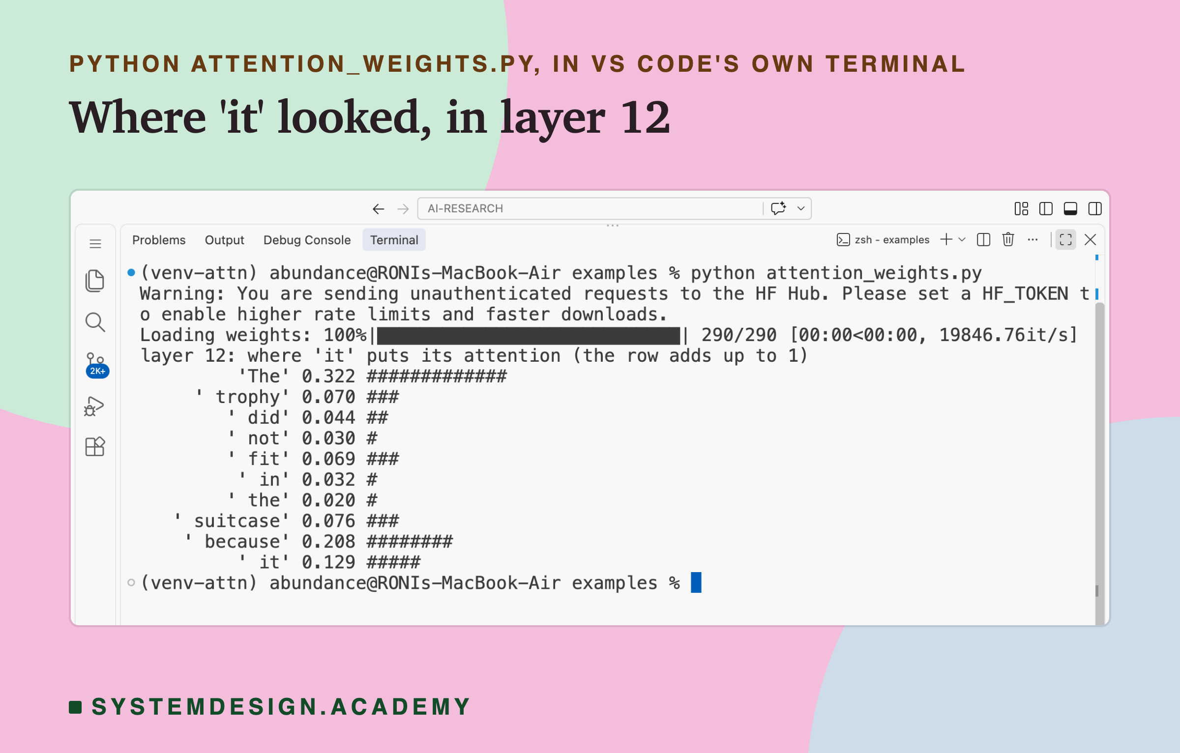
Look at the numbers. In layer 12, averaged over its 14 heads, "it" gave 0.322 of its attention to "The", 0.208 to "because" and 0.129 to itself. It gave only 0.070 to "trophy" and 0.076 to "suitcase". This layer, averaged, does not pick either noun, and the largest share goes to the first word of the sentence.

The warning at the top is harmless. Hugging Face, the site the model is downloaded from, asks for an account token for faster downloads, but the model downloads without one.

The row for "it" is one line of a bigger table. Every word has its own row, and the rows together form a grid. This grid is for layer 12, with the 14 heads averaged.

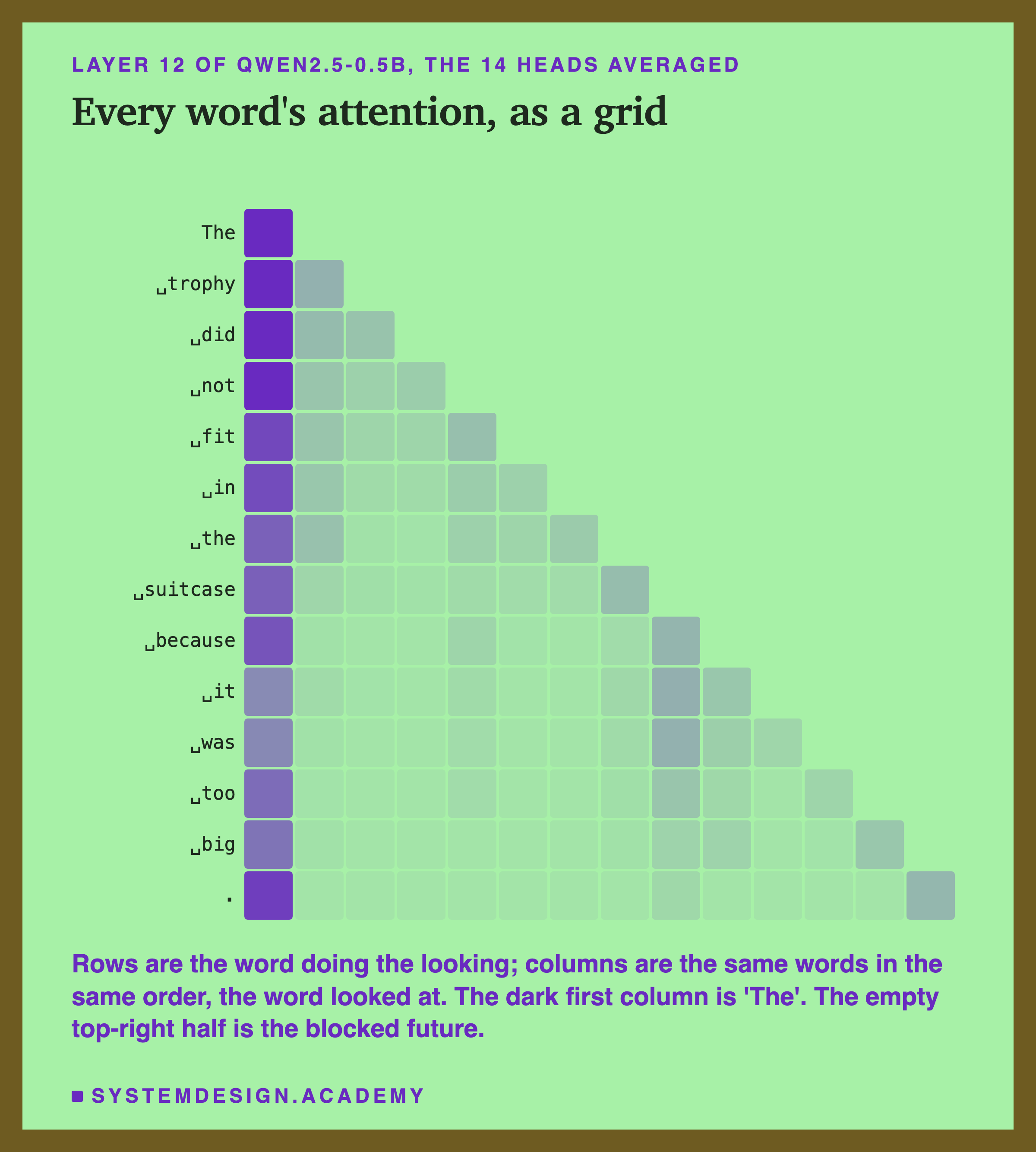
Read the grid one row at a time. Each row adds up to 1. The top-right half is empty because of the backwards-only rule. And the first column, the word "The", is dark in almost every row. That is not special to this sentence, as the next slide shows.

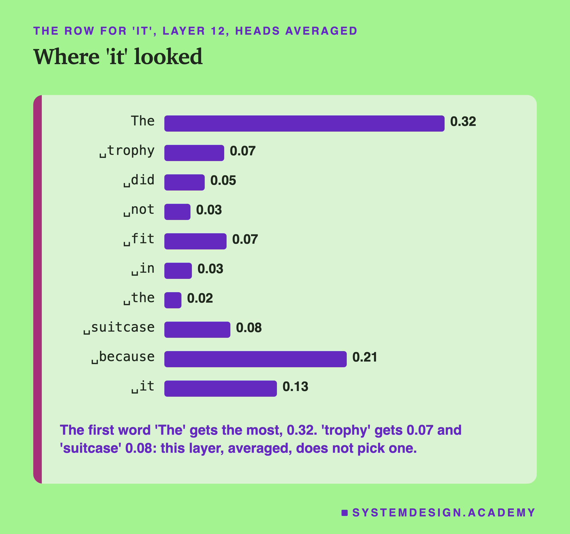
The bars show the same row as the terminal, drawn to scale. Two more things are worth noticing in the grid. First, the diagonal, where each word looks at itself: after the first word, a word's largest share often goes to itself, for example "fit" 0.15, "suitcase" 0.16 and the final full stop 0.18. Second, the column for "because" is darker in the rows below it. In this layer, several later words, including "it" and "was", give "because" a noticeable share, which fits the idea that a word joining two parts of a sentence carries information the rest of the sentence needs.

Is the large weight on "The" a quirk of one sentence? To find out, the lab took 20 real sentences from this course's own lessons and measured, for every word after the first, how much of its attention went to the very first word. That gave 398 word positions, in each of the 24 layers.

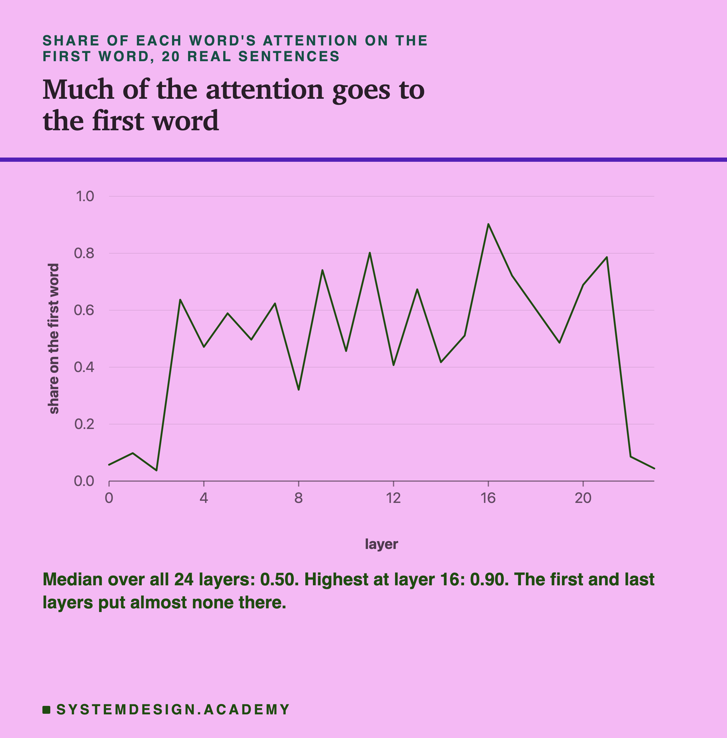
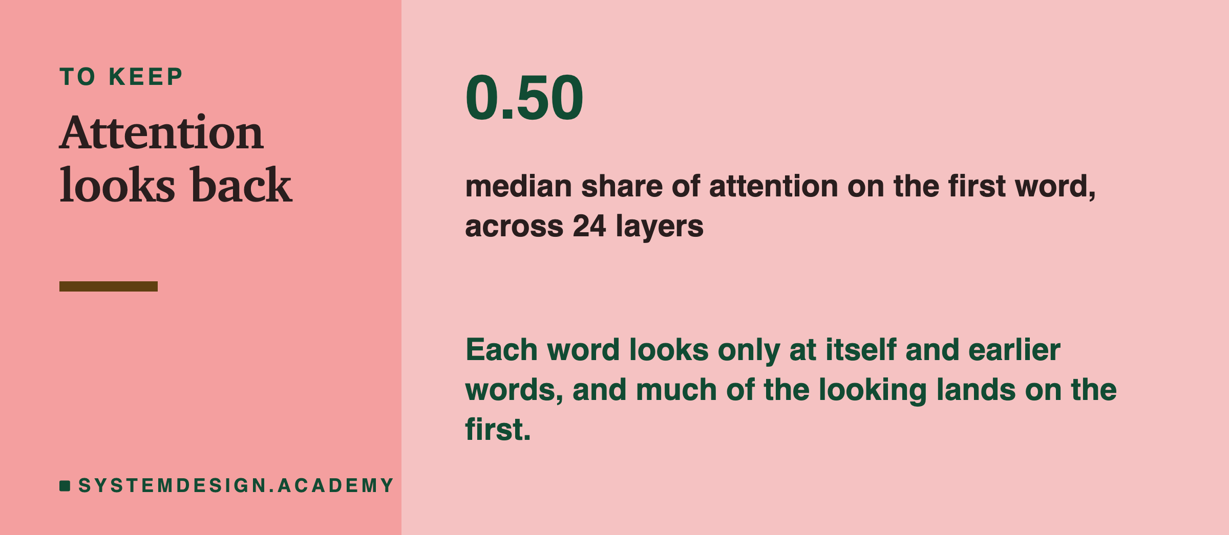
The median share, across all 24 layers, was 0.50. In other words, in a typical layer, about half of a word's attention went to the first word, whatever that word was. In layer 16 it was 0.90. Only the first three layers and the last two put little weight there.

Why would a model do that? A common explanation, which this lab did not test, goes like this. The weights must always add up to 1. When a head has nothing useful to look for in a sentence, the weight still has to go somewhere, and during training the model learns to put it on the first token, which is always present. Researchers call this an attention sink: a place where unneeded attention collects.

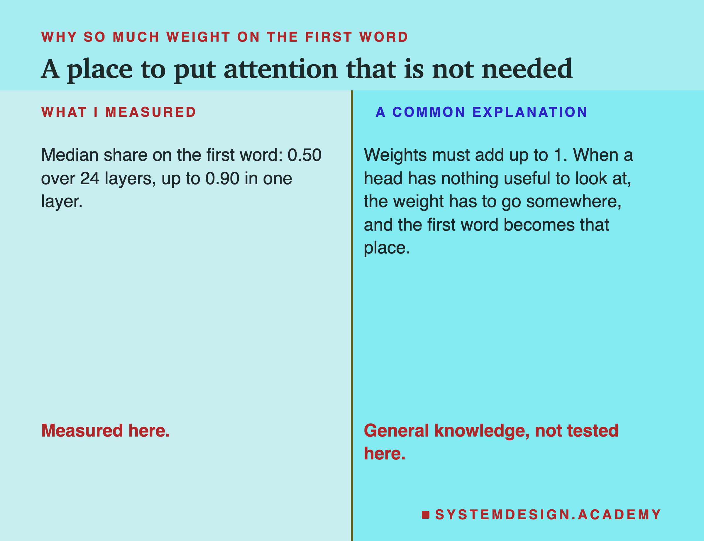
The practical point is simple. When you look at attention weights, a big weight is not automatically a meaningful one. Half the weight in a typical layer goes to a word that carries no special meaning.

The mask slide said "it" cannot see "big" or "small". The lab checked this directly.

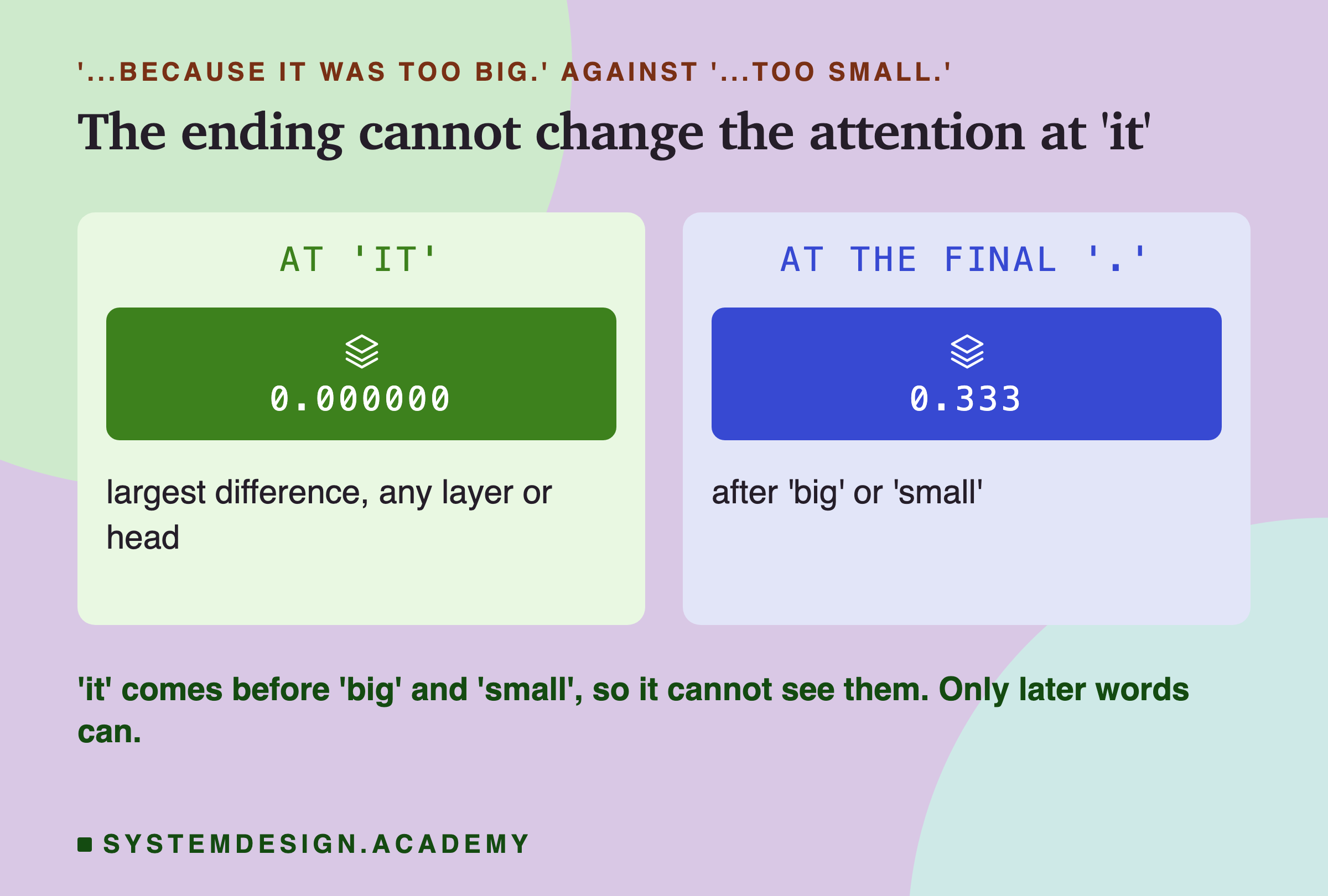
It ran both sentences, "too big" and "too small", and compared every attention weight at "it", in all 24 layers and all 14 heads. The largest difference anywhere was 0.000000. The attention at "it" was exactly the same in both sentences, as the rule predicts.

At the final full stop, which comes after the adjective, the largest difference was 0.333. The full stop can see "big" or "small", so its attention changes.

This is the clearest thing the lesson measured. Whatever the model decides about "it", it cannot decide it at "it". It has to happen later in the sentence, at words that can see both the pronoun and the clue.

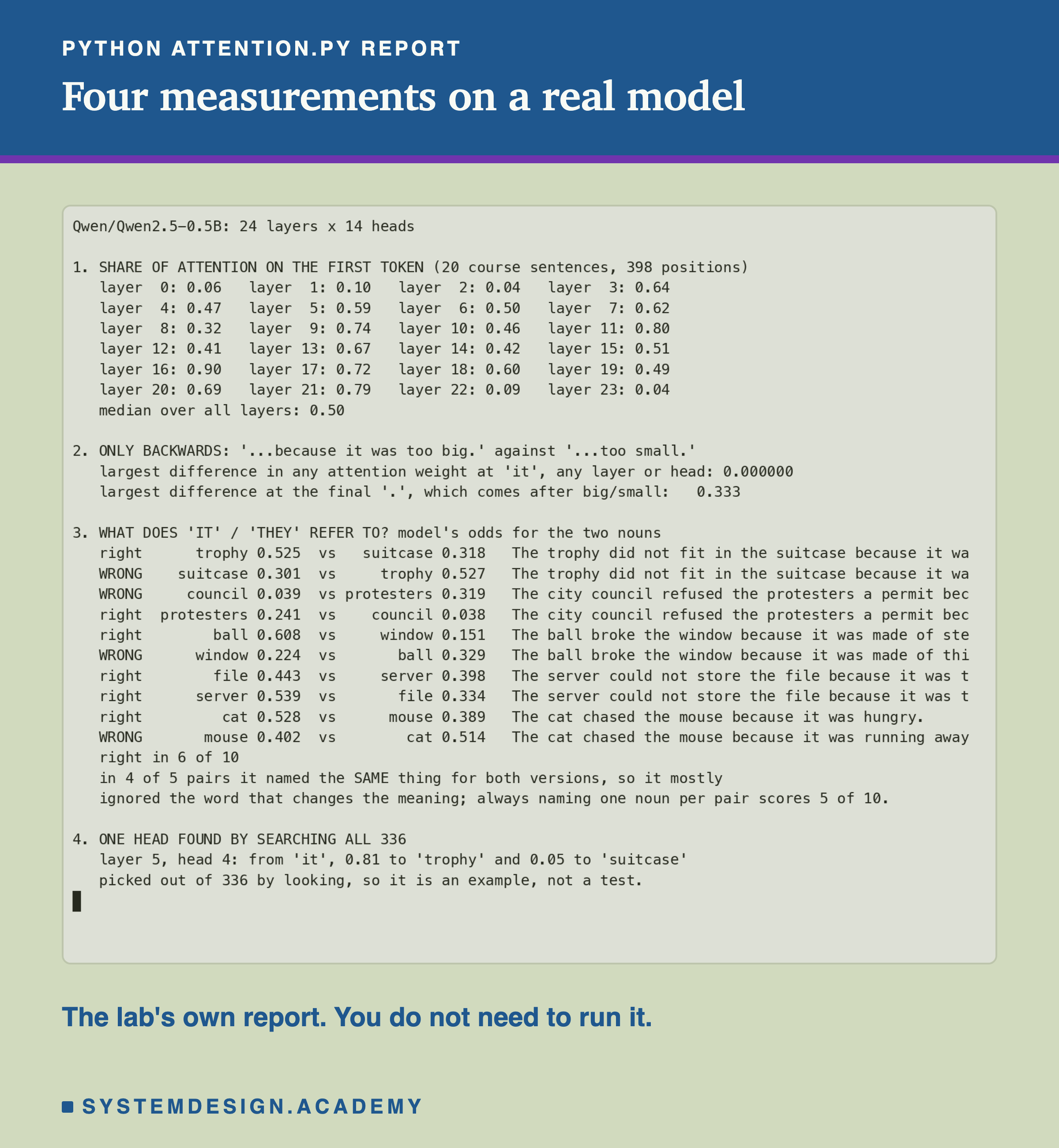
The lab, scripts/labs/generate/attention.py, makes four measurements. Section 1 is the first-word share you just saw. Section 2 is the backwards-only test. Section 3 asks whether the model resolves "it" correctly. Section 4 shows one head I found by searching. The next two slides explain sections 3 and 4.

The model was run with its "eager" attention setting, which returns every weight. The faster settings that are used in normal work compute the same result without keeping the weights. The report takes a few seconds to produce on a laptop, because the model is small and the sentences are short. Everything in it comes from one run of attention.py, saved to attention.json, so the figures in this lesson and the recording above show the same numbers.

Attention weights show where the model looked. They do not show whether it understood. So the lab asked the model directly.

It used 10 sentences, in 5 pairs. In each pair one small change flips what "it" or "they" refers to, like "too big" and "too small". After each sentence the lab added a question, "what does 'it' or 'they' refer to? Answer: the", and read the model's odds for the two nouns, the method from lesson 1.

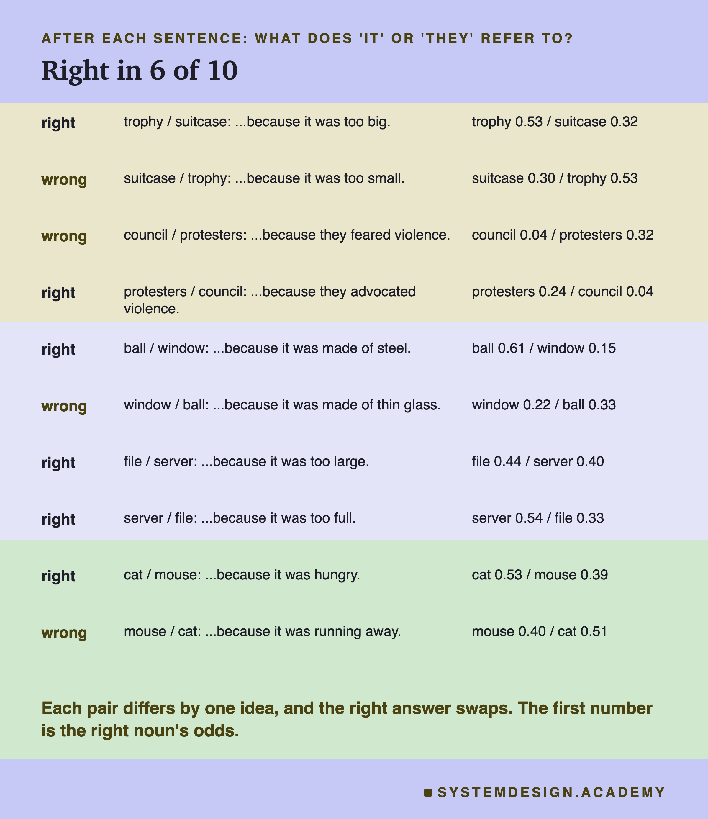
The model was right in 6 of the 10. That sounds better than guessing, but look at the pairs.

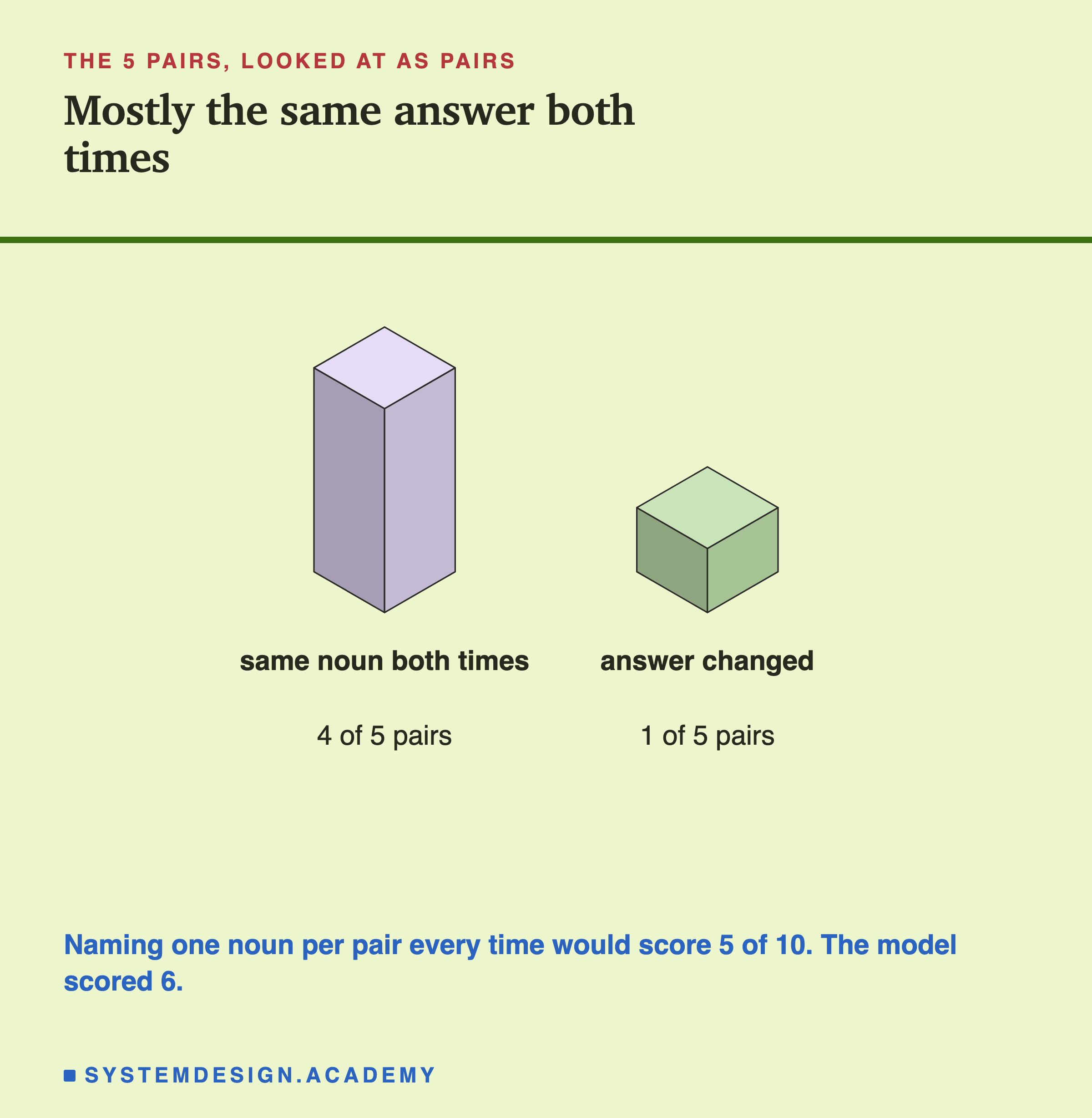
In 4 of the 5 pairs, the model gave the same noun for both versions. For the trophy pair it said "trophy" both times, and for the ball pair it said "ball" both times. In those 4 pairs it got one right and one wrong, because it gave the same noun both times. Only one pair, the server and the file, changed its answer the way it should. A model that ignored the clue completely and always named one noun per pair would score 5 of 10. This one scored 6.

This is a small model, with 0.5 billion parameters, the learned numbers inside it, and 10 sentences is a small test. Larger models are generally much better at this kind of question, though this lab did not test one. But it is a useful warning: getting some answers right is not the same as understanding the clue.

Here is the most tempting picture in the lab, and why you should be careful with it.

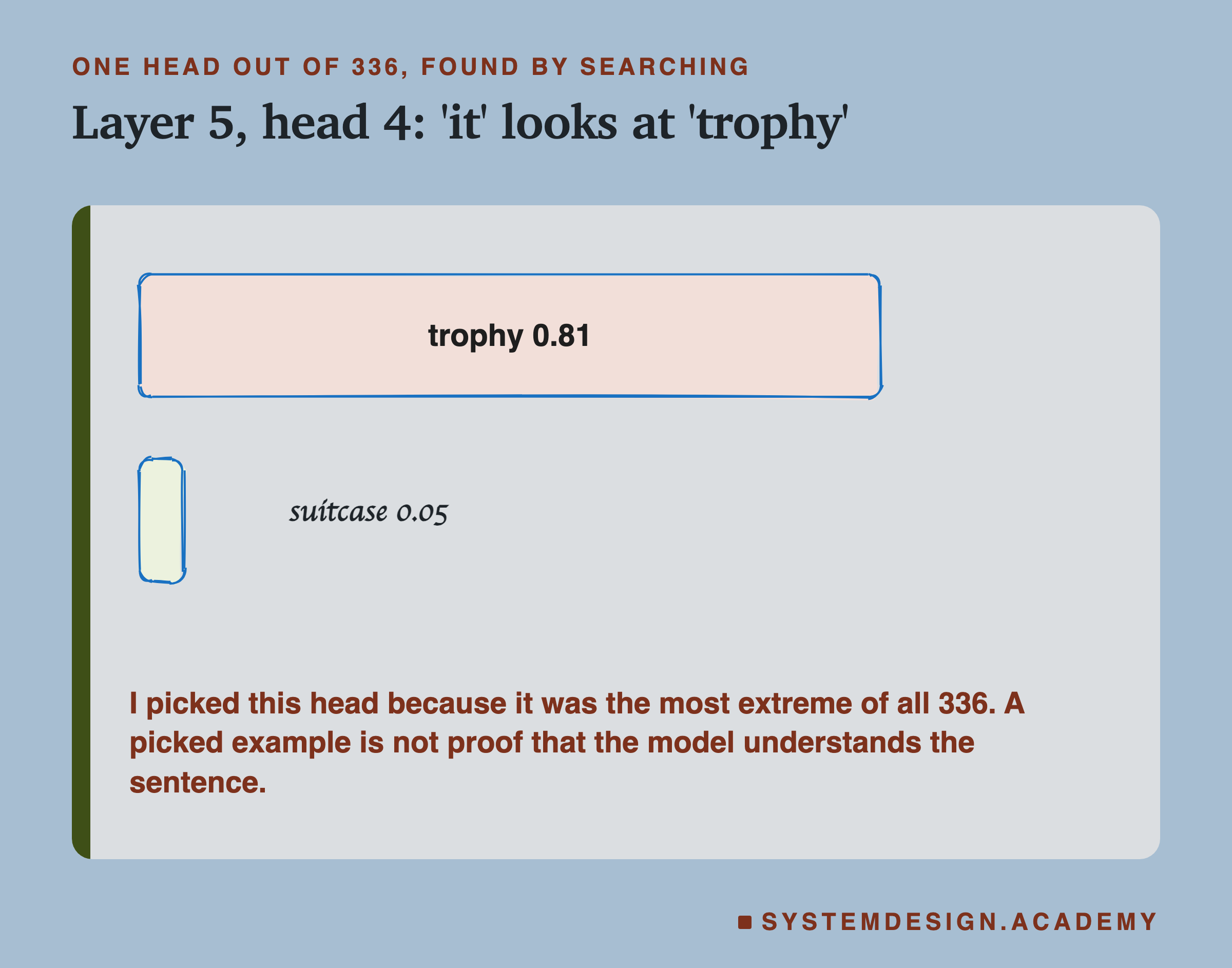
I searched all 336 heads for the one where "it" gave the most weight to "trophy" compared with "suitcase". Layer 5, head 4 gives 0.81 to "trophy" and 0.05 to "suitcase". It looks like a head that knows "it" means "trophy".

But I chose it by looking at all 336 and keeping the most extreme one. With that many heads, some will point at "trophy" by chance or for reasons unrelated to meaning. And remember the backwards test: at "it", this head cannot know whether the sentence ends in "big" or "small", so it points at "trophy" in both, including the sentence where the right answer is "suitcase". A picked example like this is a good way to explain attention, and a poor way to prove anything.

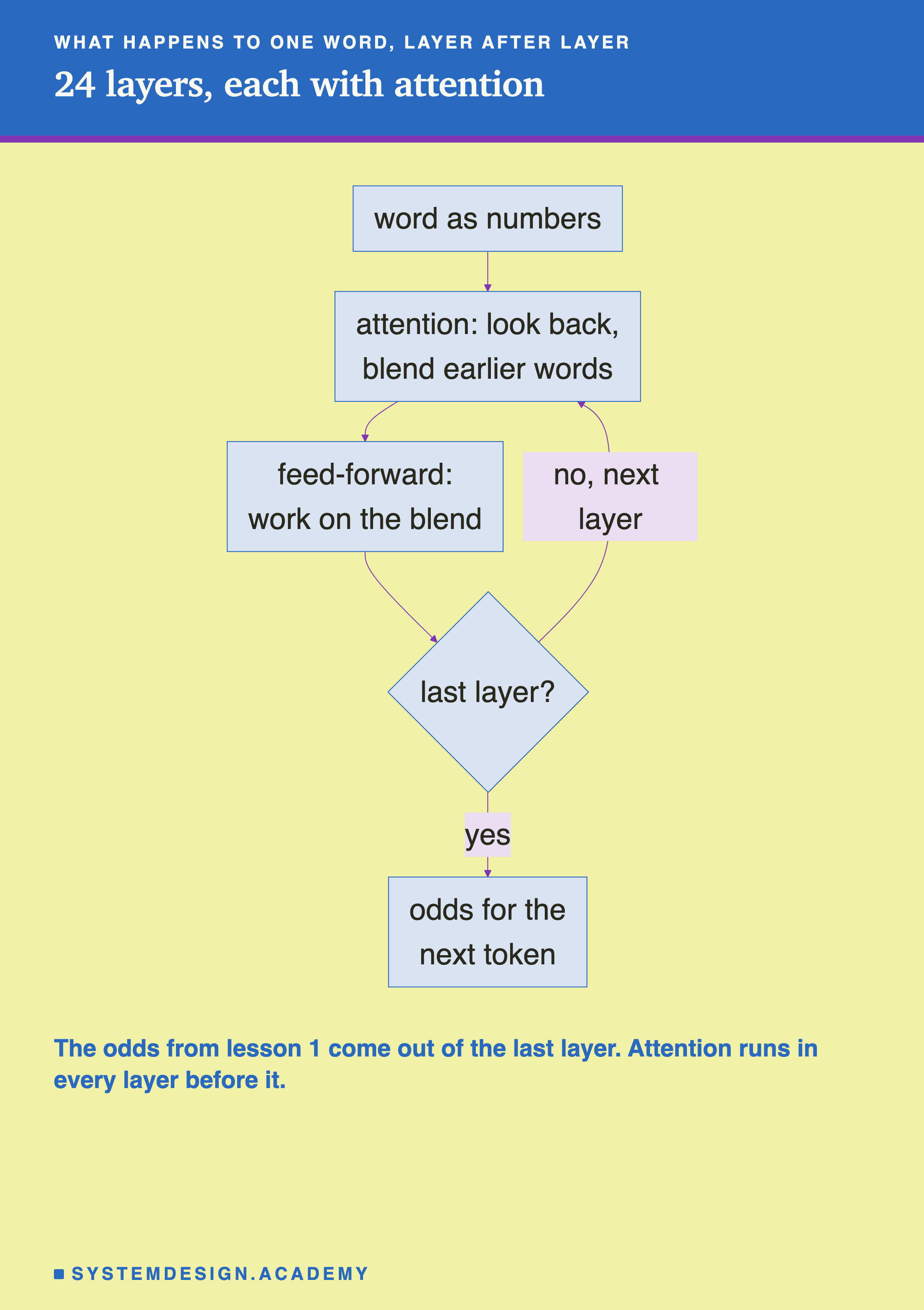
Each of the 24 layers does two things. First, attention: every word looks back and blends in the earlier words. Second, a step called feed-forward, which works on each word's blended list on its own, without looking at other words. Then the result goes to the next layer.

After the last layer, the list for the final word is turned into the odds for the next token, the odds you read in lesson 1. So every token the model writes has passed through 24 rounds of looking back.

This also connects to lesson 3. When reading a prompt, all the words go through each layer together, so the looking-back can be computed for all of them at once. When writing, each new word needs its own pass through all 24 layers, one word at a time, which is the sequential work that made writing the slow half in lesson 3.

This box does the hand calculation from earlier in Python, with no libraries. Change the query or a key and watch the weights move.

When you press Run, it prints the same four scores and weights as the hand calculation, 0.14, 0.38, 0.23 and 0.25, and the output [0.51, 0.37]. Try making the query [0.0, 1.0], so "it" is looking only for what "sat" offers most, and see the largest weight move to "sat". The last line is fixed text, so it will not change when you change the numbers; read the weights instead.

Loading. AutoTokenizer and AutoModelForCausalLM from the transformers library download the model's tokenizer and weights from Hugging Face. attn_implementation="eager" picks the plain way of computing attention, which can hand back the weights.

Running. tok(SENTENCE, return_tensors="pt") turns the sentence into token ids. model(**ids, output_attentions=True) runs all 24 layers and also returns every attention table. torch.no_grad() tells PyTorch not to keep the extra bookkeeping it would need for training, which saves memory.

Reading. out.attentions is a list with one entry per layer. Each entry is a block of numbers (PyTorch calls it a tensor) with three sides, heads × words × words: for every head, a full table like the grid on the earlier slide. [LAYER][0] picks one layer and the first (and only) sentence. .mean(dim=0) averages along the first side, the 14 heads. [pos] picks the row for "it".

Printing. The loop stops at pos, because the weights after that position are the blocked future and are all 0.

The lab. attention.py does the same reading at scale. For section 1 it loops over 20 sentences and all layers. For section 2 it runs the two trophy sentences and subtracts their weight tables at "it". For section 3 it adds the question to each sentence and reads the odds of the two nouns, the way lesson 1 read the odds for "Paris". For section 4 it subtracts, in every head, the weight on "suitcase" from the weight on "trophy" and keeps the largest.

Attention pictures are popular, and it is easy to read too much into them.

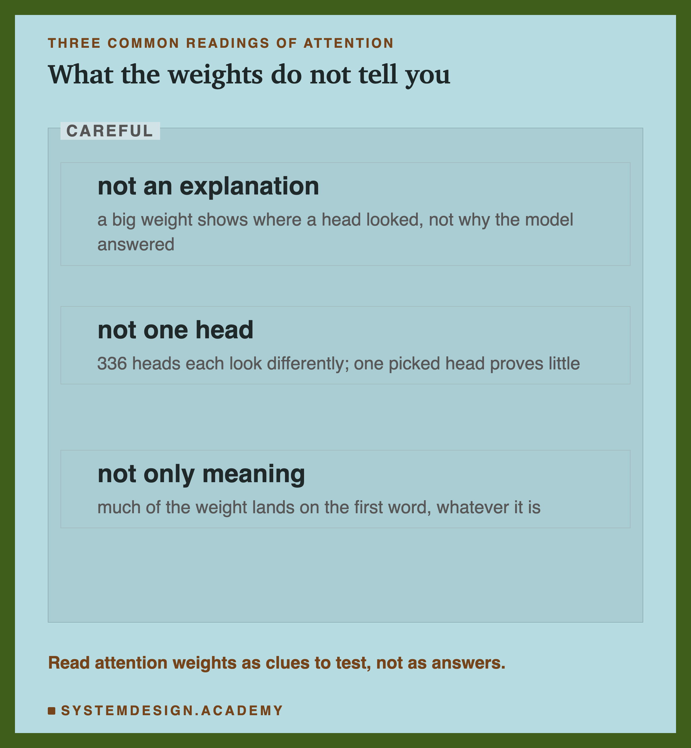
A weight is not a reason. A head can look strongly at "trophy" while the model still gives the wrong answer, as happened in the "too small" sentence. The answer comes from all 24 layers together, including the feed-forward steps, not from one weight.

One head is not the model. With 336 heads, you can almost always find one that seems to show what you hoped to see. Look at averages, or test a head across many sentences, before you believe it.

Big is not meaningful. Half the weight in a typical layer went to the first word. Look past that column, or you will wrongly think the word "The" matters most in every sentence.

Thinking a word can use words that come after it. In the models of this chapter it cannot. The meaning of "it" in the trophy sentence can only be settled at later words.

Reading one layer and one head as the answer. Look across layers and heads, and test on many sentences.

Forgetting that each row adds up to 1. A weight of 0.07 on "trophy" looks tiny. But the first word takes 0.32, and the other nine words share the remaining 0.68, about 0.076 each on average, so 0.07 is an ordinary share, not a sign that "trophy" was ignored.

Forgetting the division by √d. Here d means the number of numbers in each query and key list, and √d is its square root. In the hand calculation, skipping the √2 changes the scores and so the weights. Almost all models of this kind divide by √d.

Trusting a picked example. If you searched to find it, say so, as this lesson does for layer 5, head 4.

Using a fast attention setting and expecting weights. The default fast settings do not return the weights. Use attn_implementation="eager" when you want to read them.

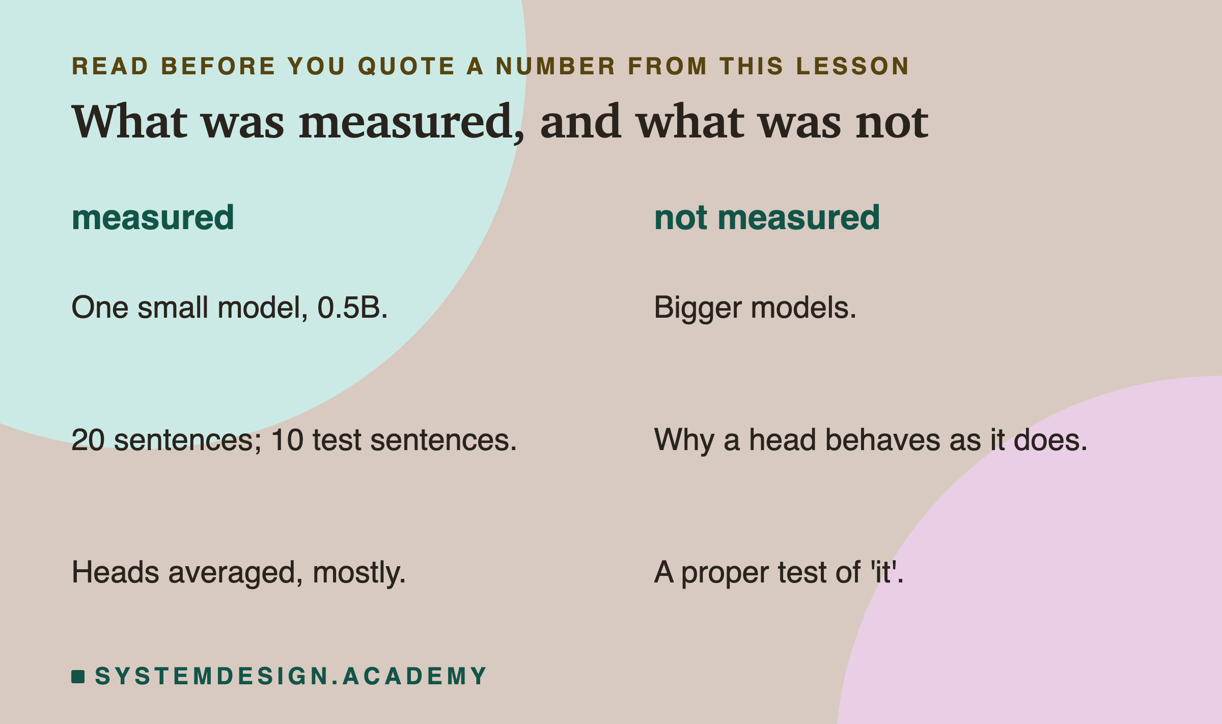
The lab looked at one small model, Qwen2.5-0.5B, with 20 real sentences for the first-word share and 10 made-up test sentences for the meaning of "it". Most results average the 14 heads of a layer.

It did not look at bigger models, where the patterns and the accuracy on sentences like the trophy pair can be quite different. It did not explain why any head behaves as it does. And 10 sentences is far too few for a proper test of whether a model resolves pronouns; it is enough only to show that this small model often did not.

Everything ran on a laptop with free tools: the model from Hugging Face, and Python with PyTorch and transformers.

Run attention_weights.py, then change LAYER and look at how the row for "it" changes from layer to layer. Try your own sentence, and try two sentences that differ by one word, the way the lab did. Every time a weight looks meaningful, ask whether it would survive the same test on ten more sentences. A good first exercise: set LAYER = 0 and then LAYER = 16, and compare how much of the row goes to the first word. The lab's chart says it should be small in layer 0 and large in layer 16.

The next lesson measures what a long prompt costs: how long the first word takes, whether writing slows down, and how much memory the model sets aside.