You can read a page of a book in a minute or two. Copying the same page out by hand takes much longer, because you have to write every word, one after another, and you cannot write the tenth word before the ninth.

A language model has the same two jobs. First it reads your prompt. Then it writes the reply, one token at a time. This lesson measures how long each job takes on a normal laptop, and explains why the two speeds are so different.

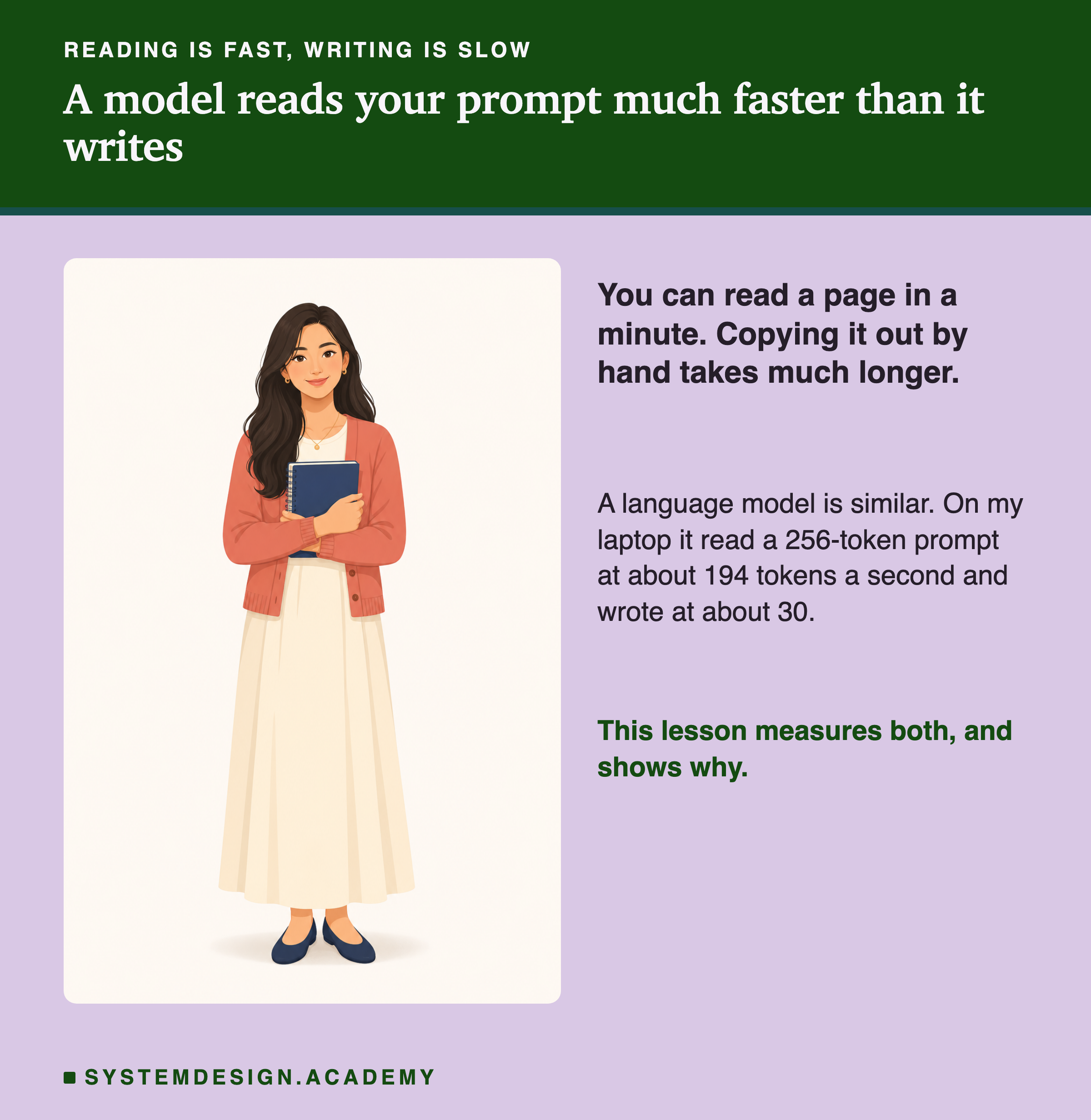
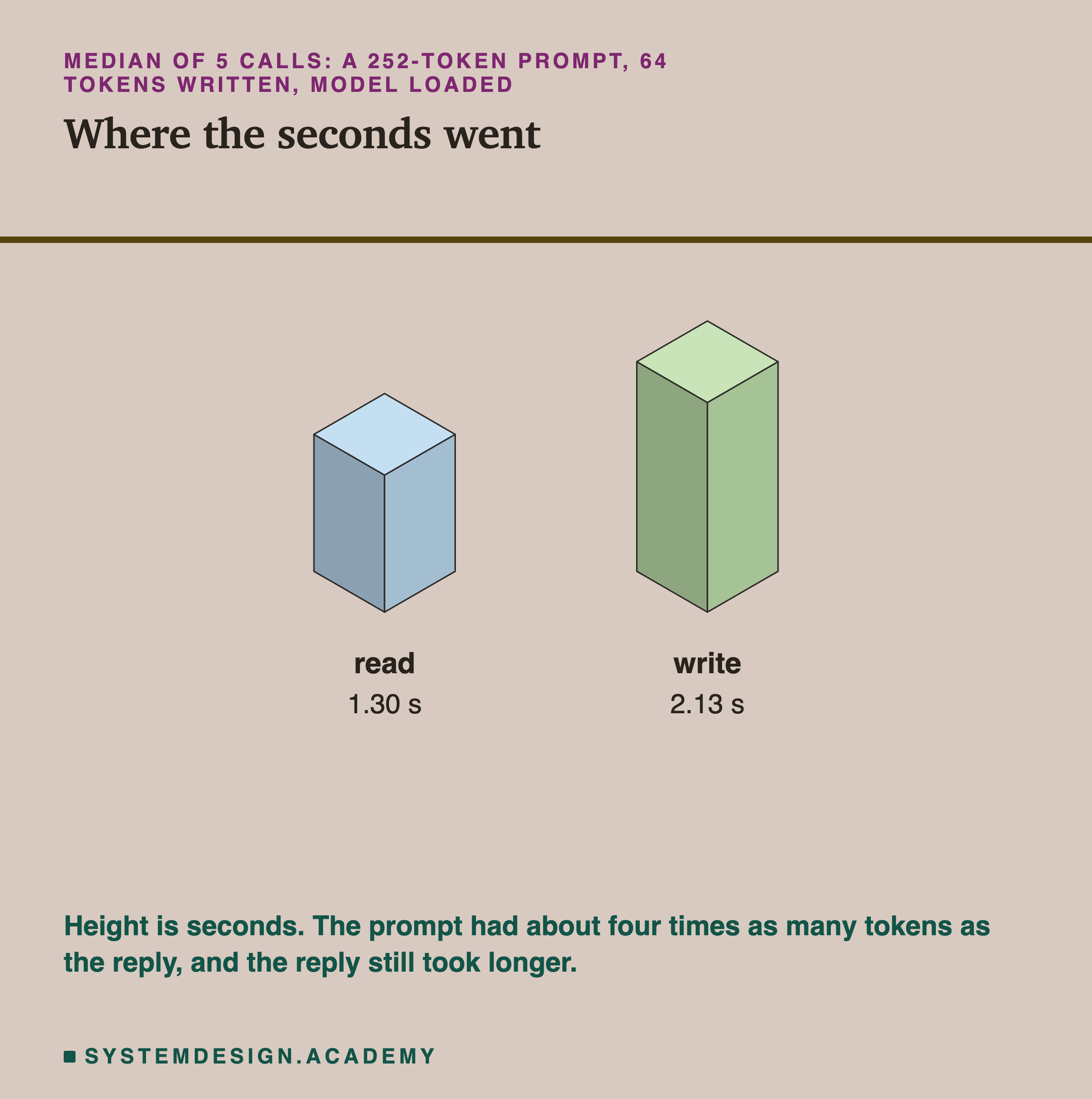
This matters because almost every decision you make when you build with a model has a time cost, and the cost is not where most people expect it. Many people think a long prompt is the slow part. On my laptop, a 1,000-token prompt was read in about 4.4 seconds, while a 192-token reply took 6.4 seconds to write. The reply, not the prompt, was where most of the time went. If you know this, you can make an app feel fast by keeping replies short and by showing words as they are written.

By the end of this lesson you will be able to read the four timings that come back with every reply, work out reading and writing speed by hand, estimate how long a call will take before you make it, and avoid the common mistakes people make when they measure speed.

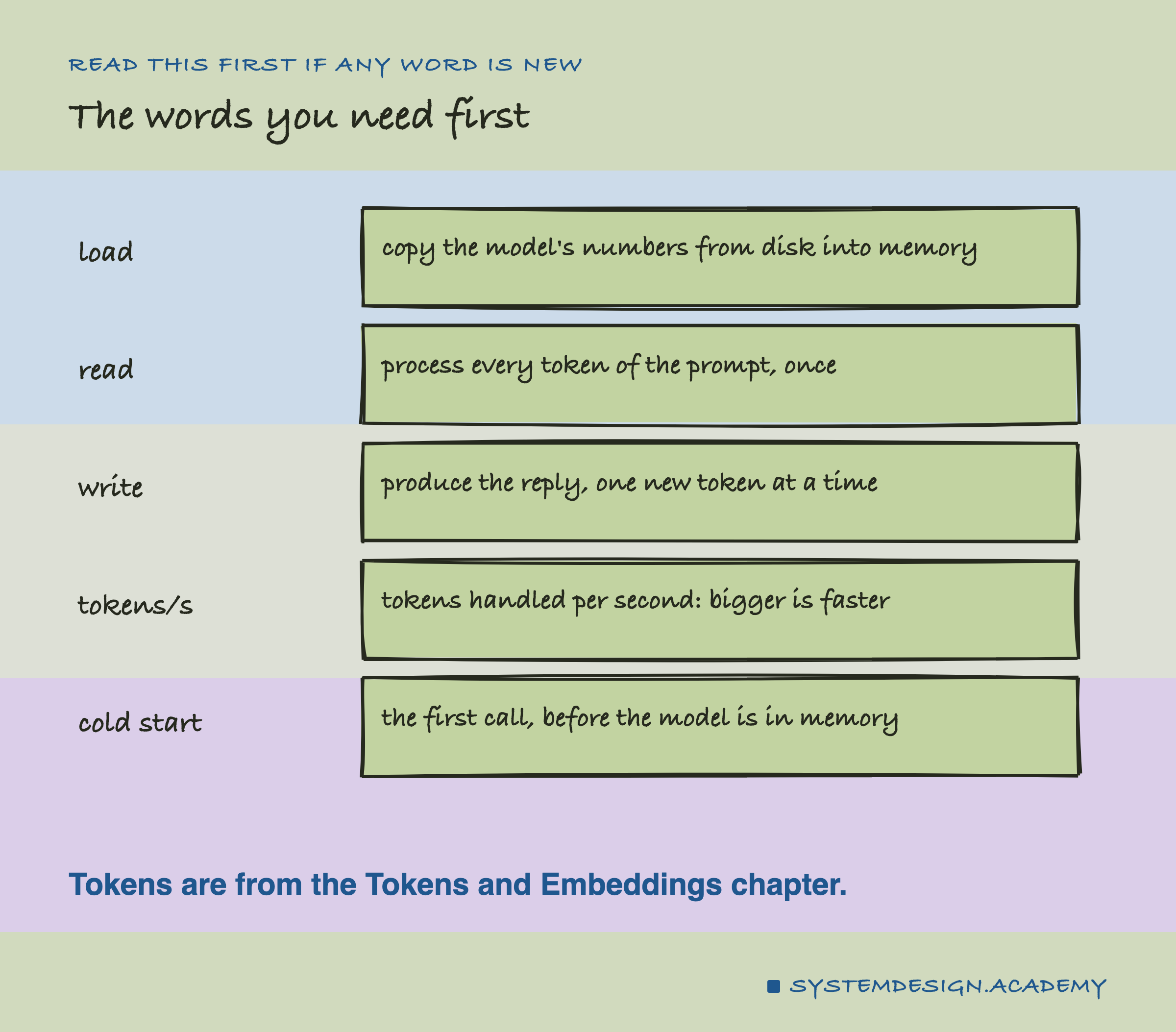
Load. Before a model can do anything, its numbers, called weights, must be copied from the disk into memory. For qwen2.5:3b that is a file of about 1.9 GB. If the file is already in memory, this takes almost no time.

Read. The model processes every token of your prompt. Engineers call this the prefill step, and Ollama calls it prompt evaluation. It happens once per call.

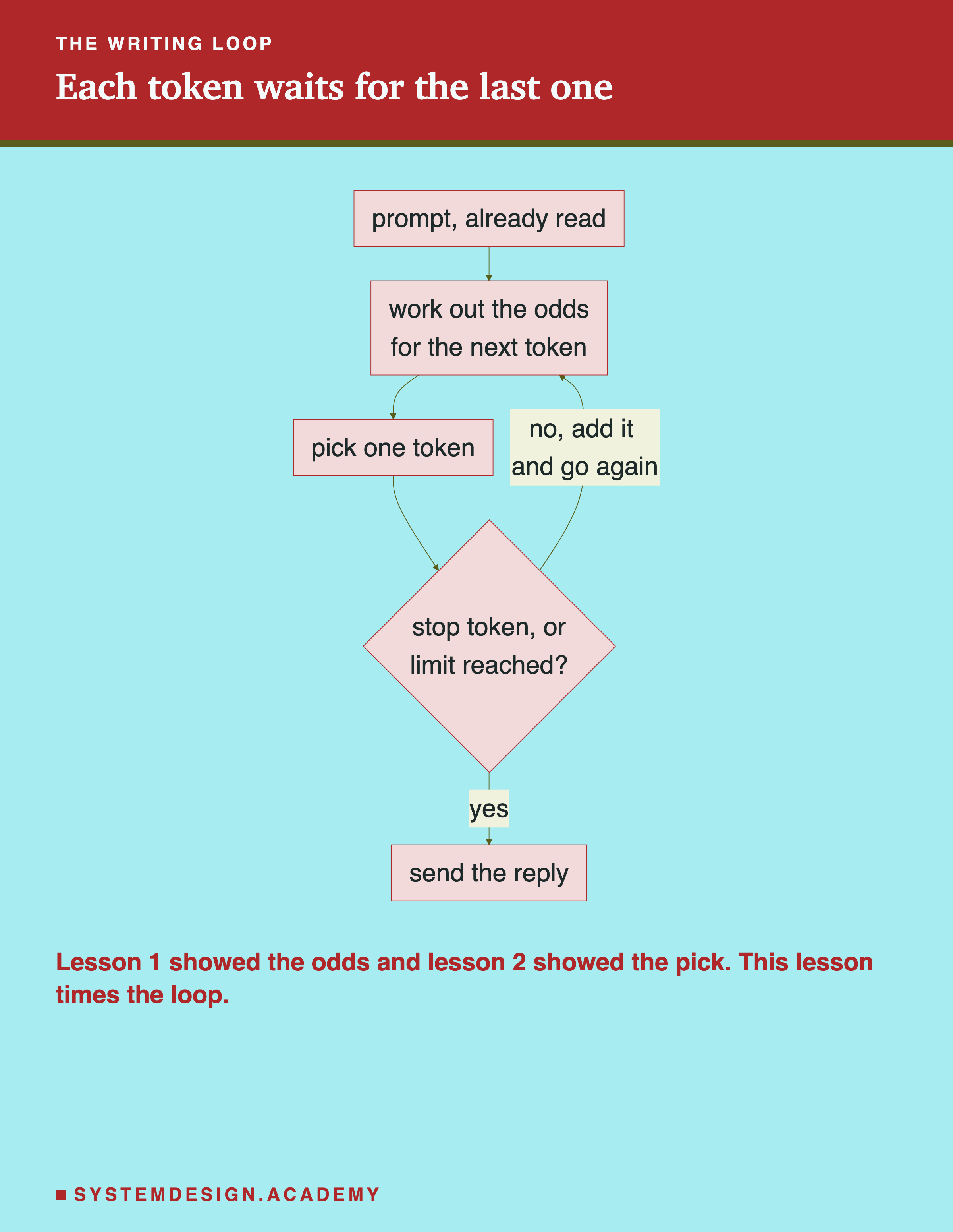
Write. The model produces the reply one token at a time. Engineers call this decoding, and Ollama calls it evaluation. Each new token is one more trip around the loop from lesson 1: work out the odds, pick a token, add it, and go again.

Tokens per second. The number of tokens handled in one second. It is the usual way to talk about speed. A bigger number is faster.

Layers and parameters. A model is built from a stack of layers, and each layer does arithmetic with a large table of learned numbers. Those numbers are the parameters, or weights. qwen2.5:3b has about 3 billion of them.

Batch. A group of items processed together in one go, instead of one at a time.

Endpoint. An address on a server that accepts requests. Ollama's /api/generate endpoint takes a prompt and returns a reply.

Latency. How long someone waits for an answer, from sending the request to getting the reply. This lesson splits latency into its parts.

Cold start. The first call after the model has been unloaded, when it still has to be loaded. Later calls are "warm".

Ollama does not only return text. Every reply from its /api/generate endpoint also carries a small set of numbers that say where the time went.

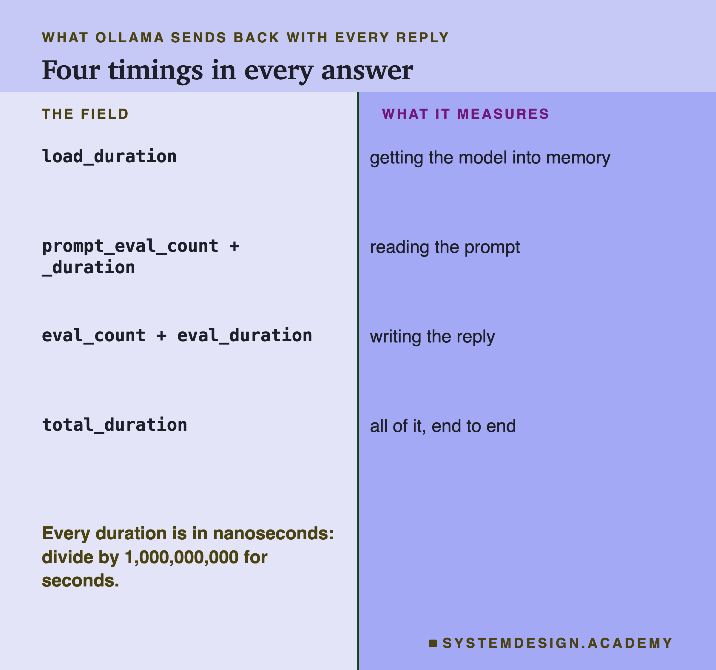
There are four groups. load_duration is the time spent getting the model into memory. prompt_eval_count and prompt_eval_duration say how many prompt tokens were read and how long that took. eval_count and eval_duration say how many tokens were written and how long that took. total_duration covers the whole request.

All the durations are in nanoseconds. A nanosecond is one billionth of a second, so you divide by 1,000,000,000 to get seconds. For example, a prompt_eval_duration of 145,722,000 nanoseconds is 145,722,000 ÷ 1,000,000,000 = 0.146 seconds.

Once you have a count and a duration, speed is a single division: tokens divided by seconds. That is all the maths this lesson needs.

Here is a small script that makes one call and prints the four timings, with both speeds worked out. It uses only the Python standard library, so there is nothing to install besides Ollama and the model.

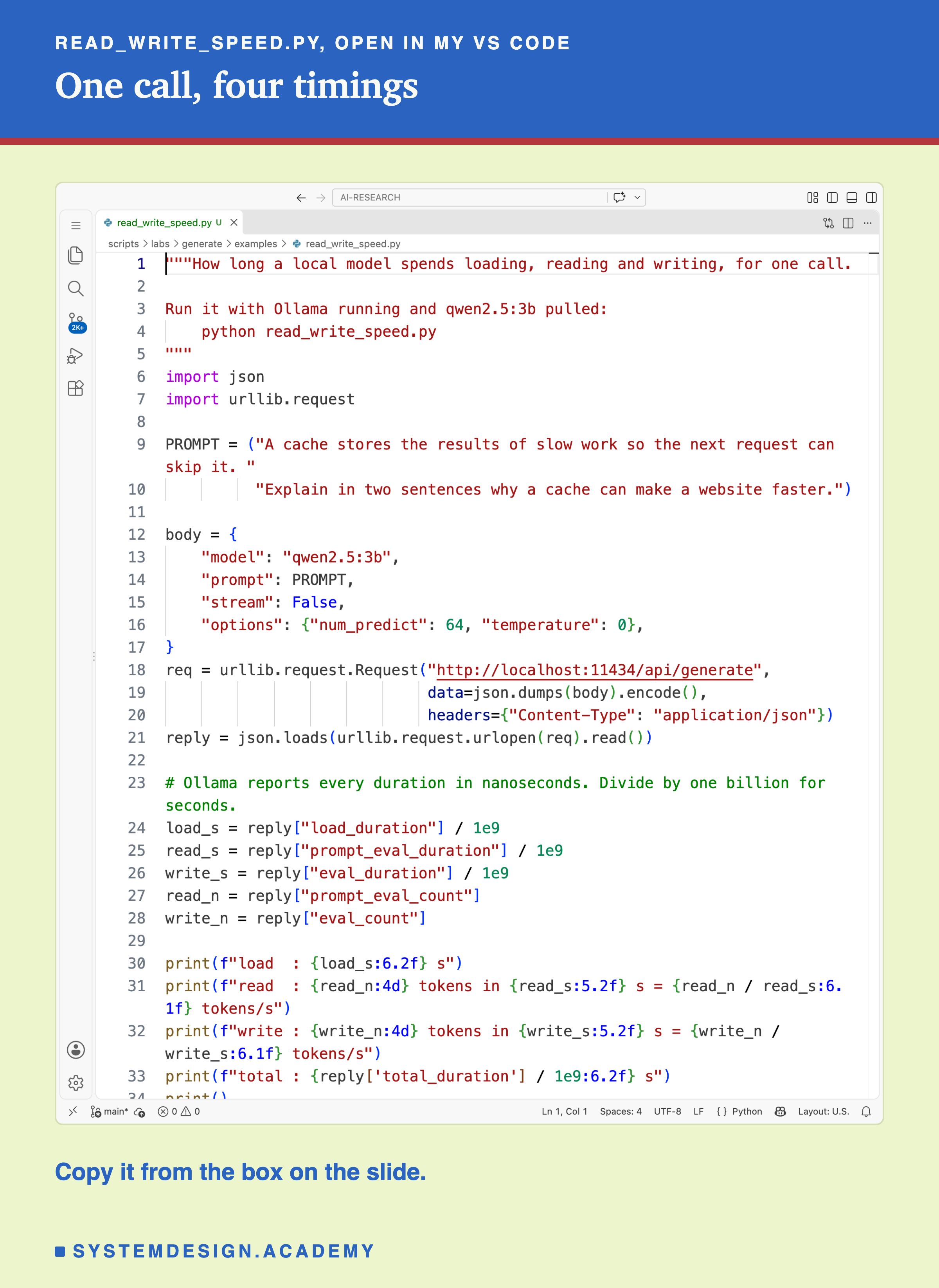
"""How long a local model spends loading, reading and writing, for one call.

Run it with Ollama running and qwen2.5:3b pulled:
    python read_write_speed.py
"""
import json
import urllib.request

PROMPT = ("A cache stores the results of slow work so the next request can skip it. "
          "Explain in two sentences why a cache can make a website faster.")

body = {
    "model": "qwen2.5:3b",
    "prompt": PROMPT,
    "stream": False,
    "options": {"num_predict": 64, "temperature": 0},
}
req = urllib.request.Request("http://localhost:11434/api/generate",
                             data=json.dumps(body).encode(),
                             headers={"Content-Type": "application/json"})
reply = json.loads(urllib.request.urlopen(req).read())

# Ollama reports every duration in nanoseconds. Divide by one billion for seconds.
load_s = reply["load_duration"] / 1e9
read_s = reply["prompt_eval_duration"] / 1e9
write_s = reply["eval_duration"] / 1e9
read_n = reply["prompt_eval_count"]
write_n = reply["eval_count"]

print(f"load  : {load_s:6.2f} s")
print(f"read  : {read_n:4d} tokens in {read_s:5.2f} s = {read_n / read_s:6.1f} tokens/s")
print(f"write : {write_n:4d} tokens in {write_s:5.2f} s = {write_n / write_s:6.1f} tokens/s")
print(f"total : {reply['total_duration'] / 1e9:6.2f} s")
print()
print(reply["response"].strip())

When I ran it in VS Code's own terminal, this is what came back.

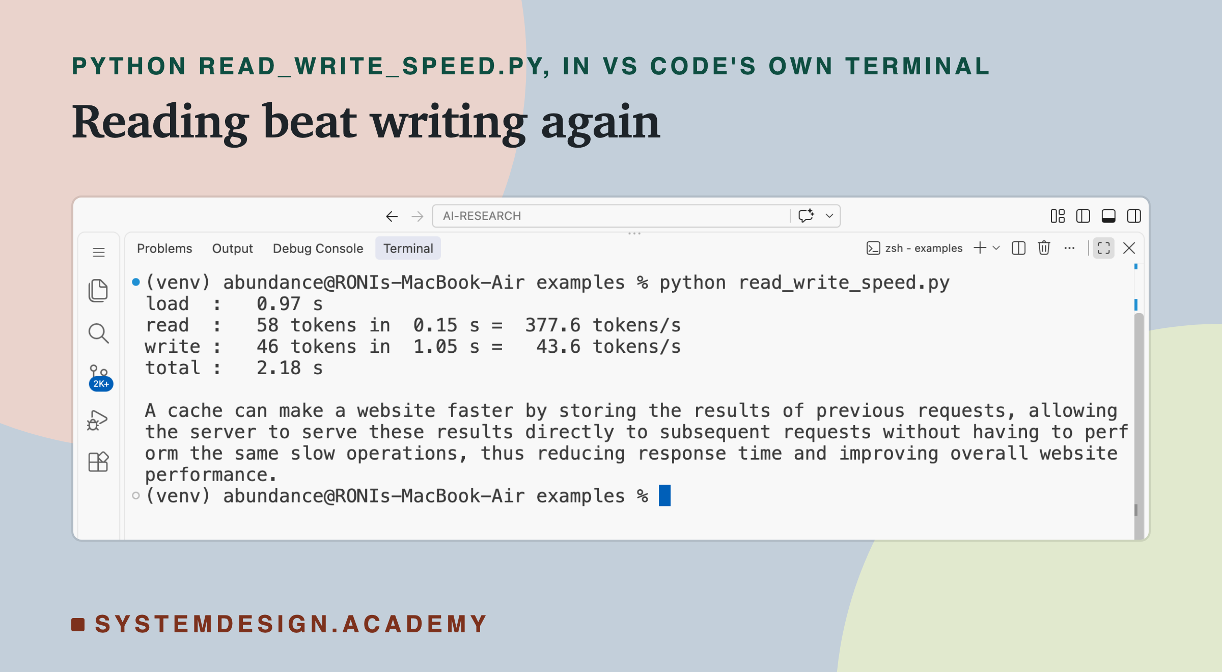
Read the three lines in the middle. Reading: 58 tokens in 0.15 seconds, about 378 tokens a second. Writing: 46 tokens in 1.05 seconds, about 44 tokens a second. So in this one call, reading was about 378 ÷ 44 ≈ 8.6 times faster per token. The model stopped at 46 tokens, before the 64-token limit, because it decided its answer was finished.

Notice one more thing. My prompt has 27 words, but the model read 58 tokens. That is because Ollama wraps a prompt in the model's chat template before the model sees it, and the template adds its own tokens. Lesson 1 showed the same effect: 5 tokens for a raw prompt, 34 once the template was added.

One call is only one call. So I measured 35 calls, in a way I describe on the lab slide, and took the median, which is the middle value once the results are sorted.

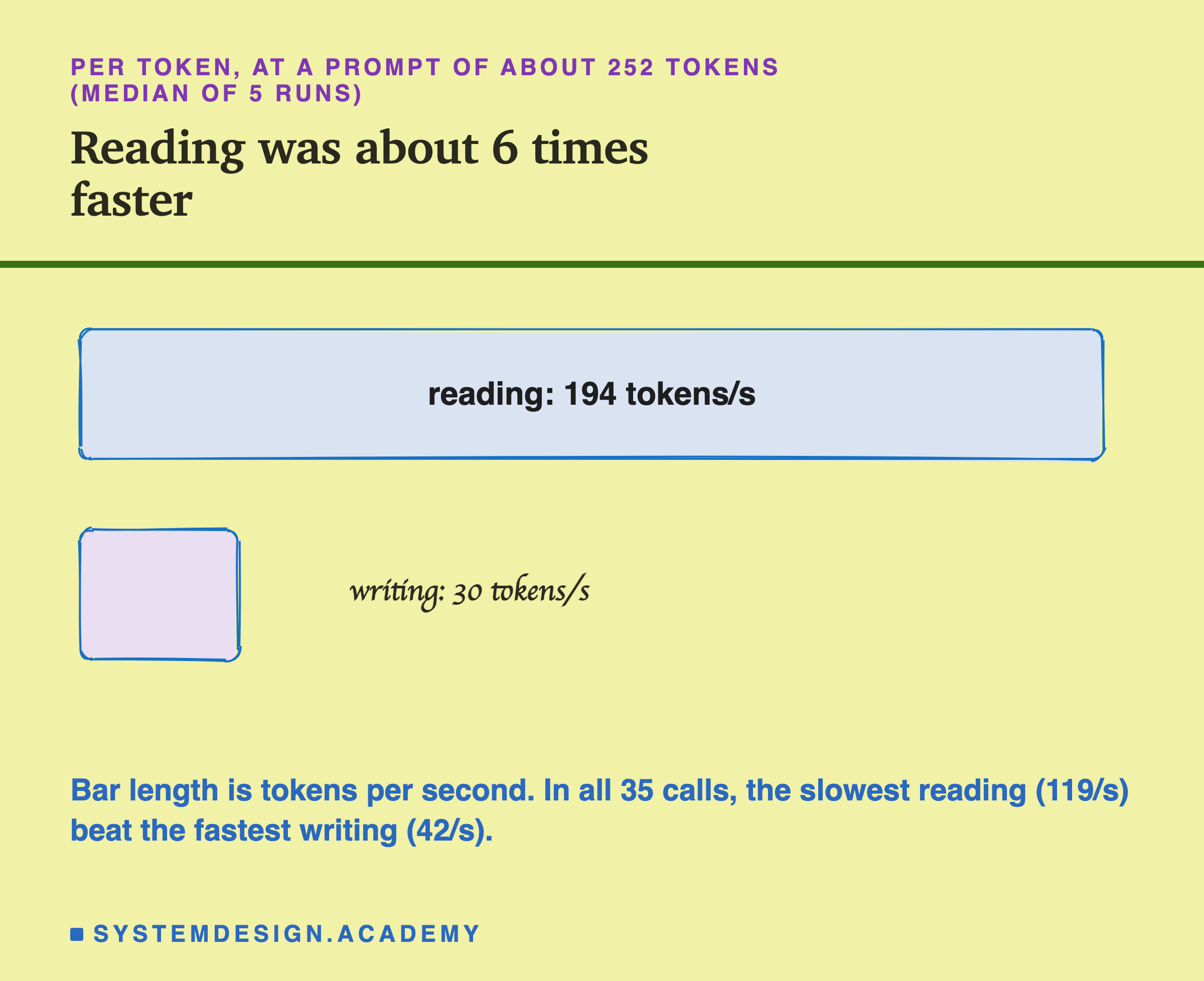
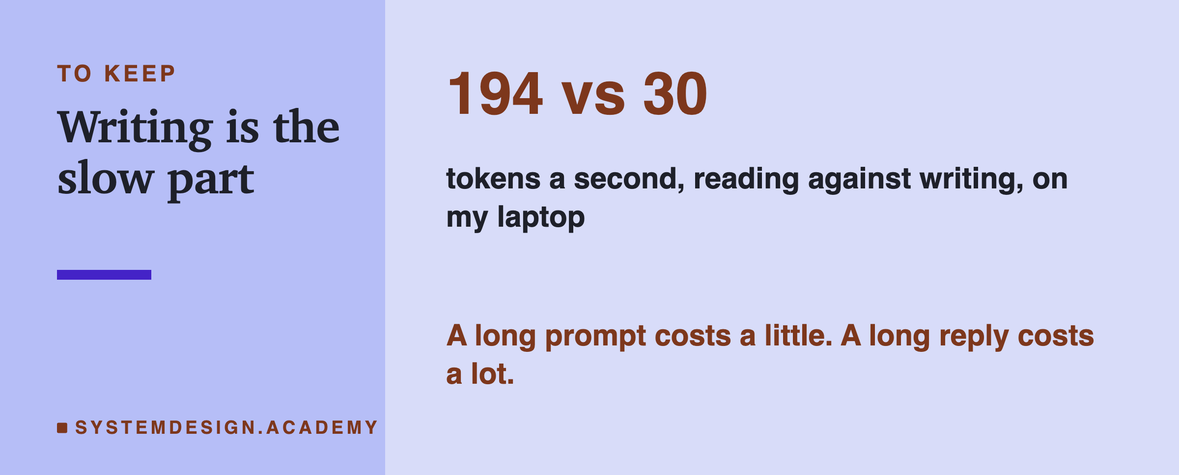
At a prompt of about 252 tokens, the median reading speed was 194 tokens a second and the median writing speed was 30. Divide one by the other: 194 ÷ 30 ≈ 6.5. So one written token took about as long as reading six or seven prompt tokens.

The medians could hide a lot, so I also checked the extremes. Across all 35 calls, the slowest reading speed of any call was 119 tokens a second, and the fastest writing speed of any call was 42. Even the worst reading beat the best writing, by 119 ÷ 42 ≈ 2.8 times. This is the part of the result I trust most, because it held in every single call, whatever else the laptop was doing.

The exact ratio will not be the same on your machine. A different model, a different chip or a busier laptop will change both numbers. The direction, reading much faster per token than writing, is what you should expect everywhere.

The difference comes from how the work is shaped, not from the model being lazy.

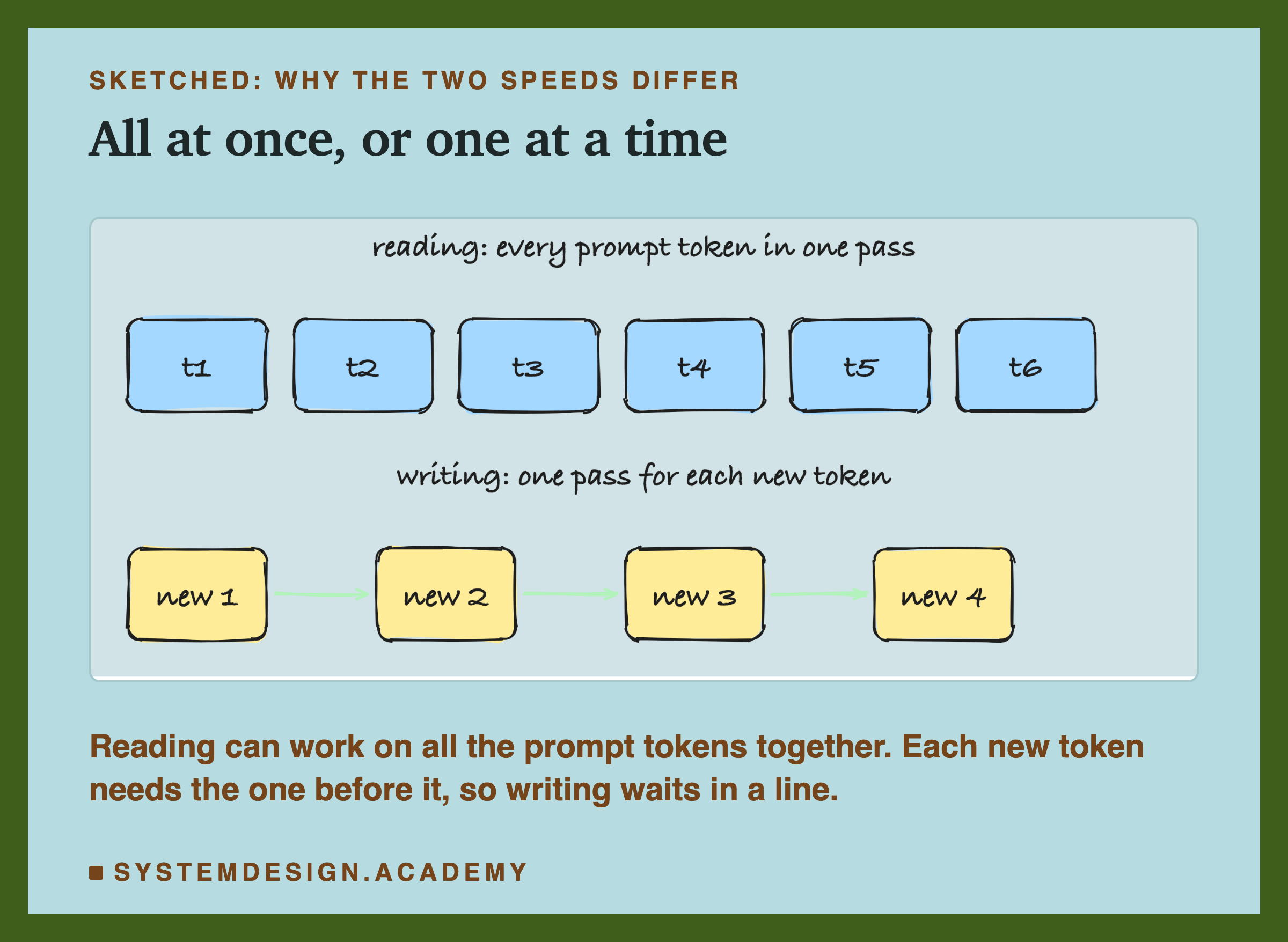
When the model reads, all the prompt tokens are already known. It can push them through its layers together, as one big batch of arithmetic. A laptop's graphics chip is built for exactly this kind of work: many multiplications at once. So reading 250 tokens costs much less than 250 separate steps.

When the model writes, it cannot work ahead. The second new token depends on the first, because the first is part of the text the model must look at to choose the second. So each written token needs its own trip through all the model's layers. That is general knowledge about how these models run, not something my lab measured directly, but it matches what the lab shows: per token, writing is several times slower.

There is a second reason, also general knowledge. For each written token, the chip has to read all of the model's weights from memory once. For a 3-billion-parameter model that is a lot of data moved for very little arithmetic, so writing is often limited by how fast memory can be read, not by how fast the chip can calculate.

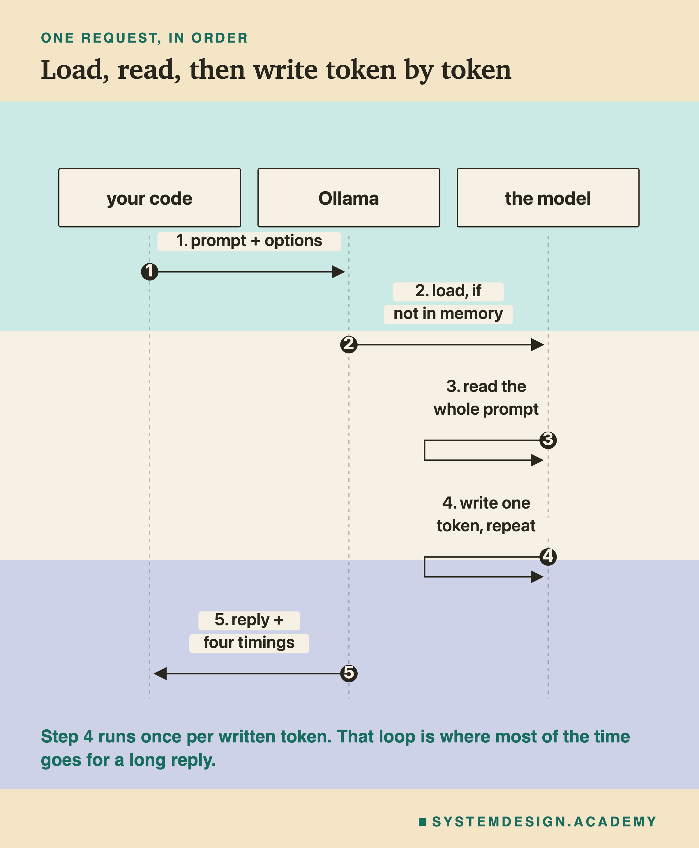
The sequence shows the order of events for one request. Steps 2 and 3 happen once. Step 4 happens once for every token in the reply, which is why the reply length matters so much.

Here is the arithmetic for one real reply, the one saved for the box further down. It is a separate call from the VS Code run above, with the same prompt, so its numbers are a little different. You can check every step with a calculator.

The fields. prompt_eval_count is 58 and prompt_eval_duration is 145,722,000 nanoseconds. eval_count is 46 and eval_duration is 1,021,285,000 nanoseconds. load_duration is 689,845,584 and total_duration is 1,858,534,084.

Step 1, seconds. Divide each duration by 1,000,000,000. Reading: 145,722,000 ÷ 1,000,000,000 ≈ 0.146 s. Writing: 1,021,285,000 ÷ 1,000,000,000 ≈ 1.021 s. Loading: about 0.690 s. Total: about 1.859 s.

Step 2, speeds. Reading: 58 ÷ 0.146 ≈ 398 tokens a second. Writing: 46 ÷ 1.021 ≈ 45 tokens a second.

Step 3, the ratio. 398 ÷ 45 ≈ 8.8. In this call, one written token cost as much time as reading almost nine prompt tokens.

Step 4, where the total went. 0.690 + 0.146 + 1.021 = 1.857 seconds. The total was 1.859, so about 0.002 seconds went to other small jobs, such as turning the prompt into tokens. Of the time that the model itself was working, writing took 1.021 ÷ (0.146 + 1.021) ≈ 0.87, or 87%.

Notice that the reply had fewer tokens than the prompt, 46 against 58, and still took about seven times as long.

One call can mislead you, so the lab, scripts/labs/generate/speed.py, measured many. It used qwen2.5:3b at temperature 0 on my Apple M4 laptop with 24 GB of memory. It sent prompts in raw mode, which skips the chat template, so the token counts are exactly the lab's text.

It ran two tests. In the reading test, the prompt grew from about 64 to about 4,096 tokens, and every call wrote 64 tokens. In the writing test, the prompt stayed at about 256 tokens, and the call was asked to write 16, 64 or 256 tokens. Each setting ran 5 times, which gives 20 reading calls and 15 writing calls, 35 in all. Then it unloaded the model three times and timed the reload.

The prompts were built from this course's own lesson text, so they read like real documents rather than a word repeated over and over.

Two details protect the numbers. First, every prompt starts with its own line, "Run 1.", "Run 2." and so on. Ollama remembers a prompt it has just read, and if the next prompt starts the same way it skips reading that part. A unique first line makes sure every prompt is read in full, and the lab checks that the token counts match. Second, all 35 calls ran in one shuffled order, not one test after the other. The next slide shows why that mattered.

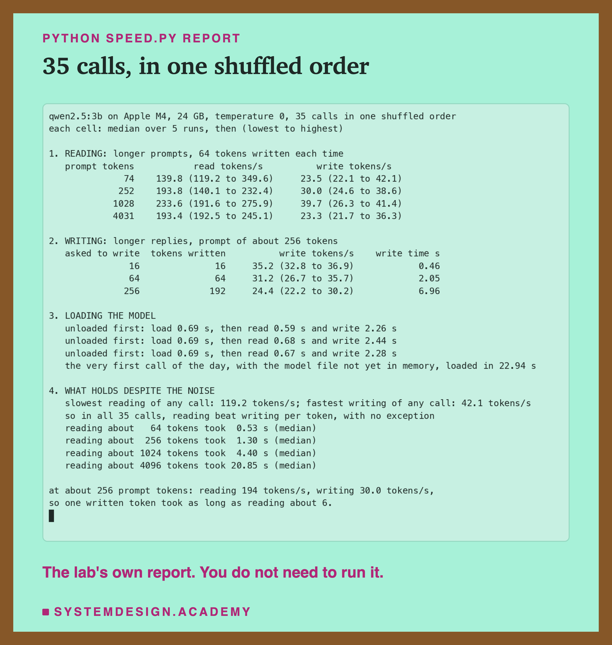
Read the report from the top. Section 1 is the reading test, section 2 the writing test, section 3 the loading test, and section 4 lists what held in every call. Each cell shows the median of 5 runs, then the lowest and highest in brackets. The brackets are wide, and the noise slide explains why.

The first question is simple: if the prompt gets longer, how much longer does the reading take?

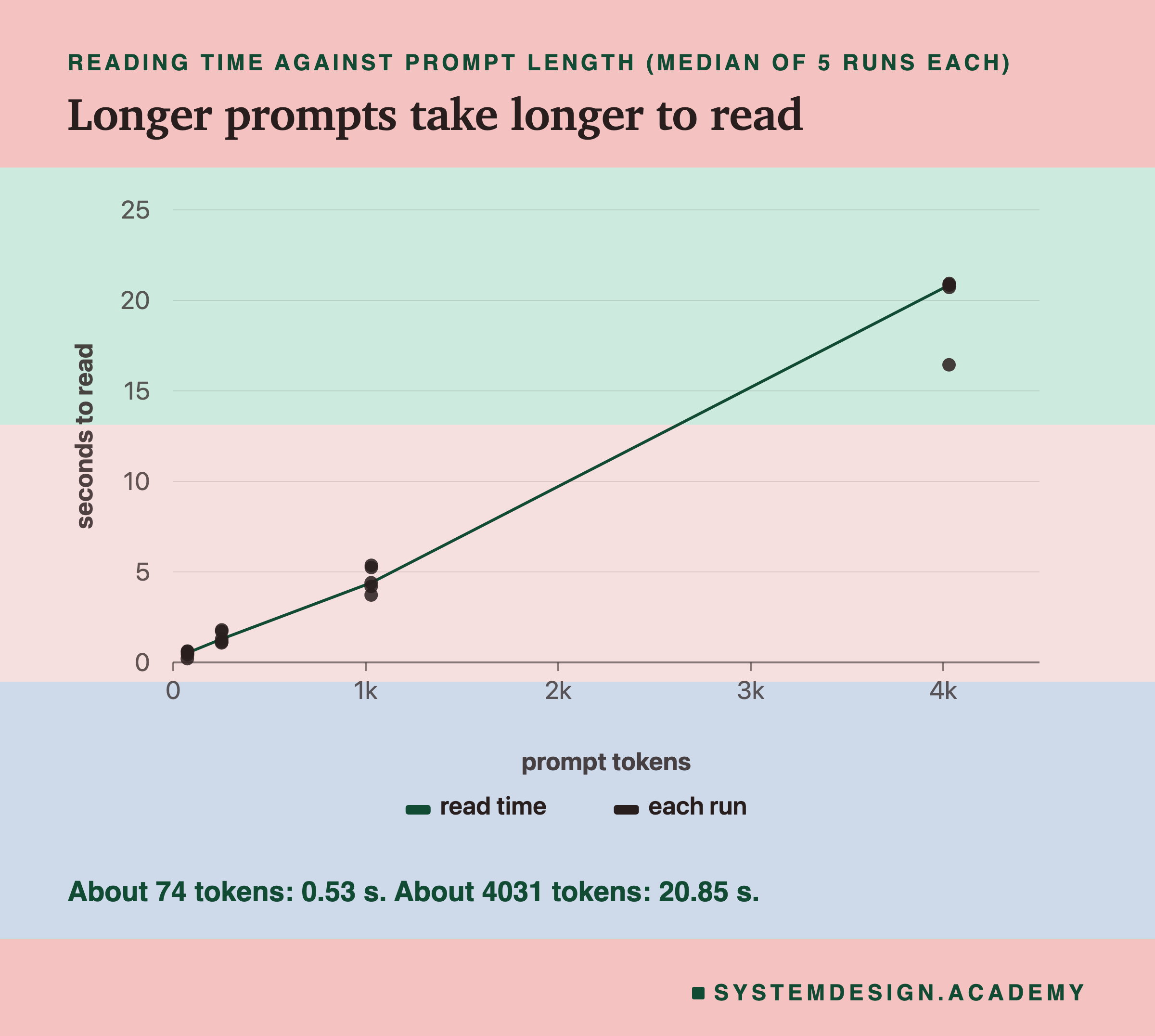
The median reading times were 0.53 seconds for about 64 tokens, 1.30 for about 256, 4.40 for about 1,024 and 20.85 for about 4,096. Reading time grows with the prompt, as you would expect.

Is the growth in proportion? At first sight the last step looks bigger: about 1,028 to about 4,031 tokens is 4,031 ÷ 1,028 ≈ 3.9 times as many, while the median time went from 4.40 to 20.85 seconds, 20.85 ÷ 4.40 ≈ 4.7 times as long. But that comparison is spoiled by the drift you will meet on the noise slide. Three of the five 1,024-token calls ran in the first ten calls, while the laptop was still fast, and only one of the five 4,096-token calls did. If you compare only calls that ran after the first ten, both lengths were read at the same speed, about 192 to 196 tokens a second. So on this laptop, above about 1,000 tokens, reading time grew roughly in proportion to the prompt.

Short prompts were a little slower per token: the 74-token prompts were read at a median of 140 tokens a second. A likely reason, which I did not measure, is that every call has some fixed work, and on a short prompt that fixed work is spread over fewer tokens.

So a very long prompt is not free. At about 4,000 tokens it took about 21 seconds on this laptop before the first word of the reply could even start. But per token, it was still read far faster than a reply is written.

The second question: if the reply gets longer, how much longer is the wait?

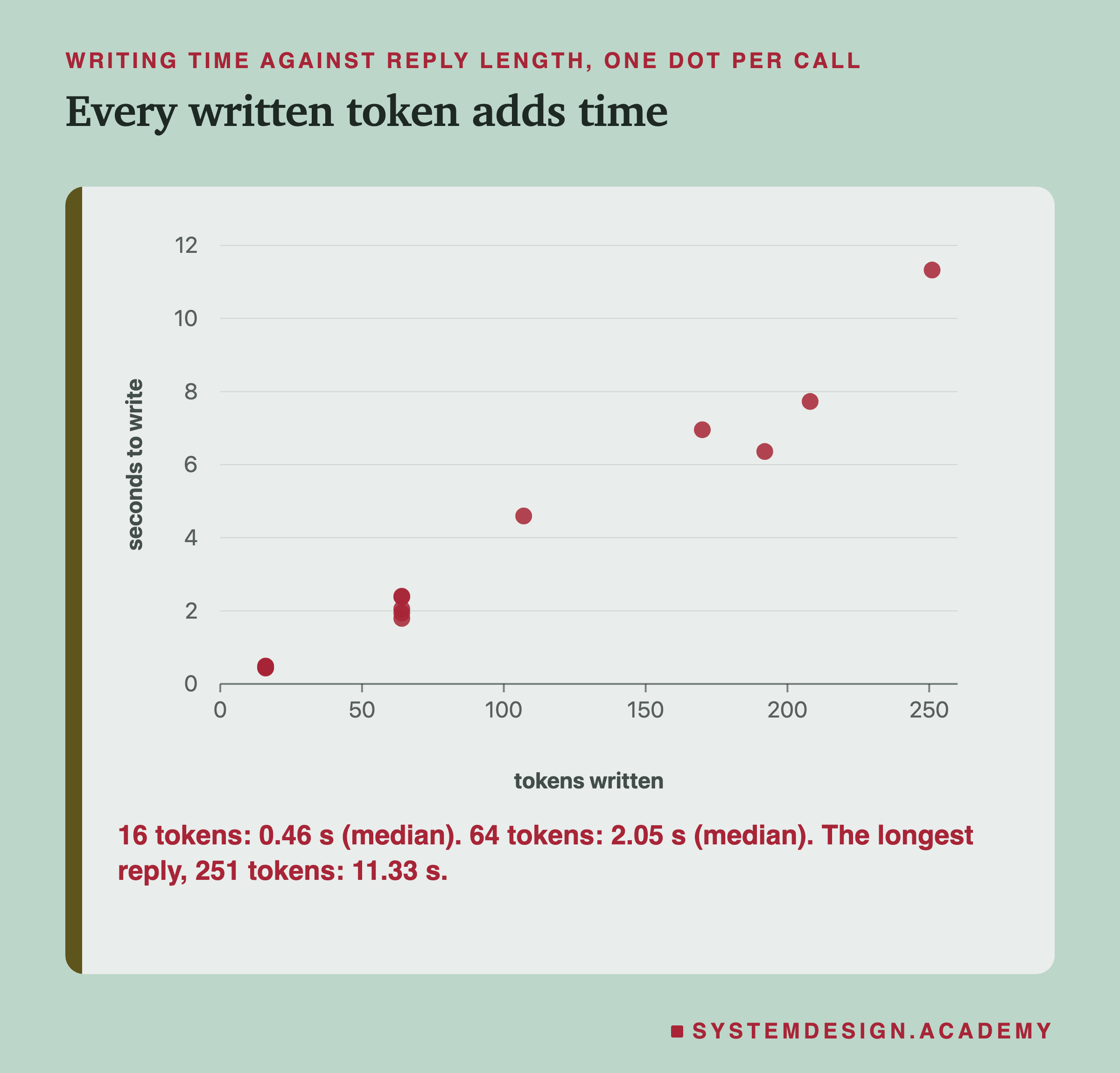
Each dot is one real call. The median writing times were 0.46 seconds for 16 tokens and 2.05 seconds for 64. The calls asked for 256 tokens did not all write 256: the model stopped on its own when it thought the answer was finished, so those five replies were 107, 170, 192, 208 and 251 tokens long. Their times were 4.60, 6.96, 6.36, 7.73 and 11.33 seconds.

The dots lie close to a straight line: more tokens, proportionally more time. From 16 to 64 tokens is 4 times as many, and 2.05 ÷ 0.46 ≈ 4.5 times as long. The 192-token reply took 6.36 seconds, which is 6.36 ÷ 2.05 ≈ 3.1 times as long as 64 tokens for 3 times as many tokens. Per token, the 16-token replies ran at a median of about 35 tokens a second and the 64-token replies at about 31, but the drift on the next slide is big enough that I would not trust that small difference.

The simplest way to make a reply faster is to make it shorter. Asking for "two sentences" instead of "a detailed explanation", or setting num_predict to cap the length, cuts the wait almost directly.

My first version of this lab ran the tests one after the other: all the reading calls, then all the writing calls. The writing speed at the same 256-token prompt came out at 40.9 tokens a second in the first block and 28.9 in the second. Same model, same prompt size, different answer.

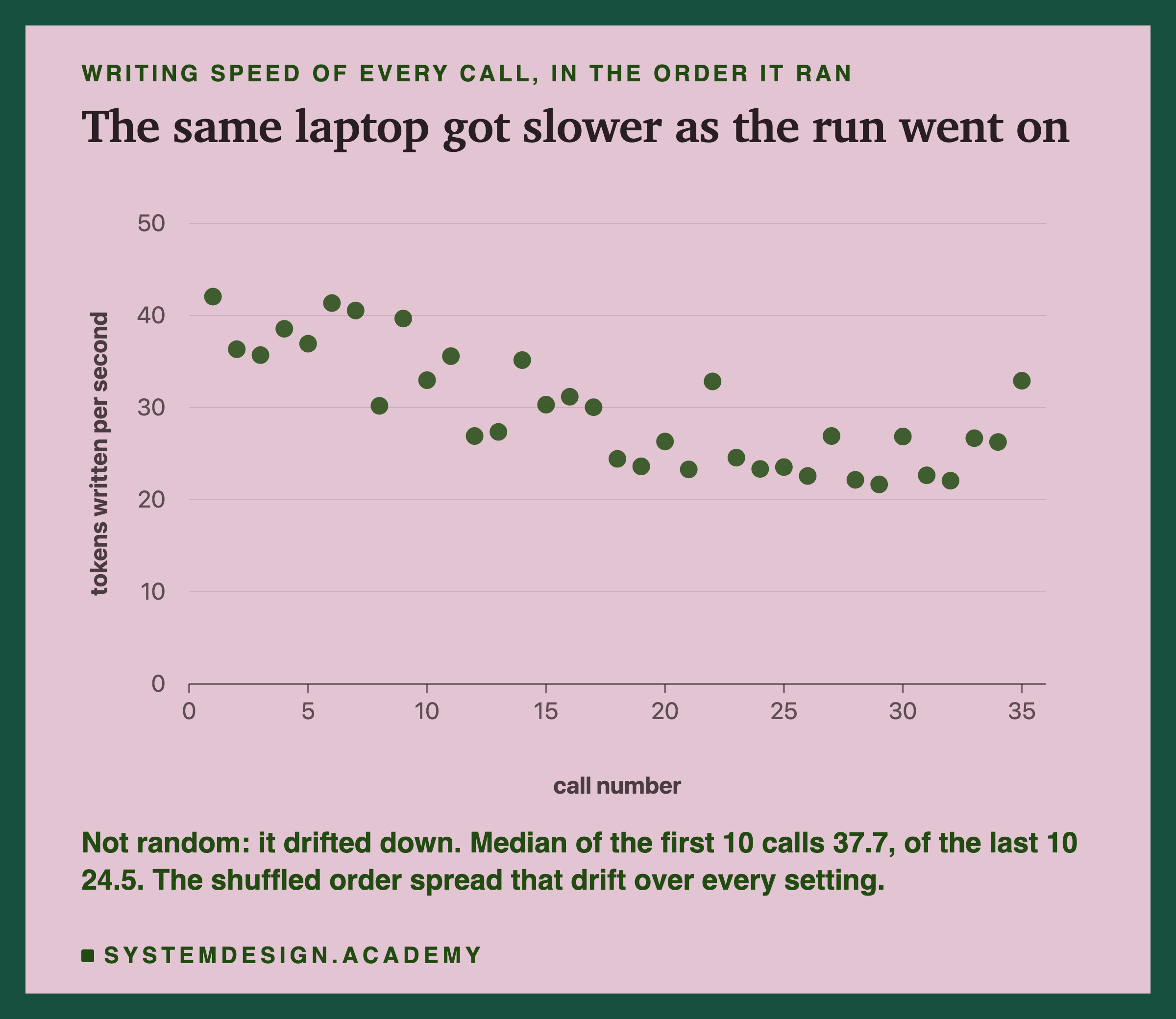
The chart shows what happened in the final run. The laptop got slower as the run went on: the median writing speed of the first 10 calls was 37.7 tokens a second, and of the last 10 it was 24.5. I do not know the exact cause. The laptop's temperature log showed no warnings, but other programs were busy at the same time, including the photo-analysis and search-indexing services macOS runs in the background, and the editor I was working in.

This drift is why the order was shuffled. If the reading test runs first and the writing test second, the drift makes writing look slower than it is. When all 35 calls are mixed in one random order, each setting gets some early, fast calls and some late, slow ones, so the drift spreads evenly instead of pretending to be a difference between settings. The random order used a fixed seed, 7, so the lab can be repeated exactly.

Three habits come out of this. Shuffle the order of the settings you compare. Repeat each setting several times and report the median and the range, not one number. And prefer a claim that holds in every call, like "the slowest reading beat the fastest writing", over a claim that depends on a small difference between medians.

Once you know the two speeds on your machine, you can predict how long a call will take, before you make it.

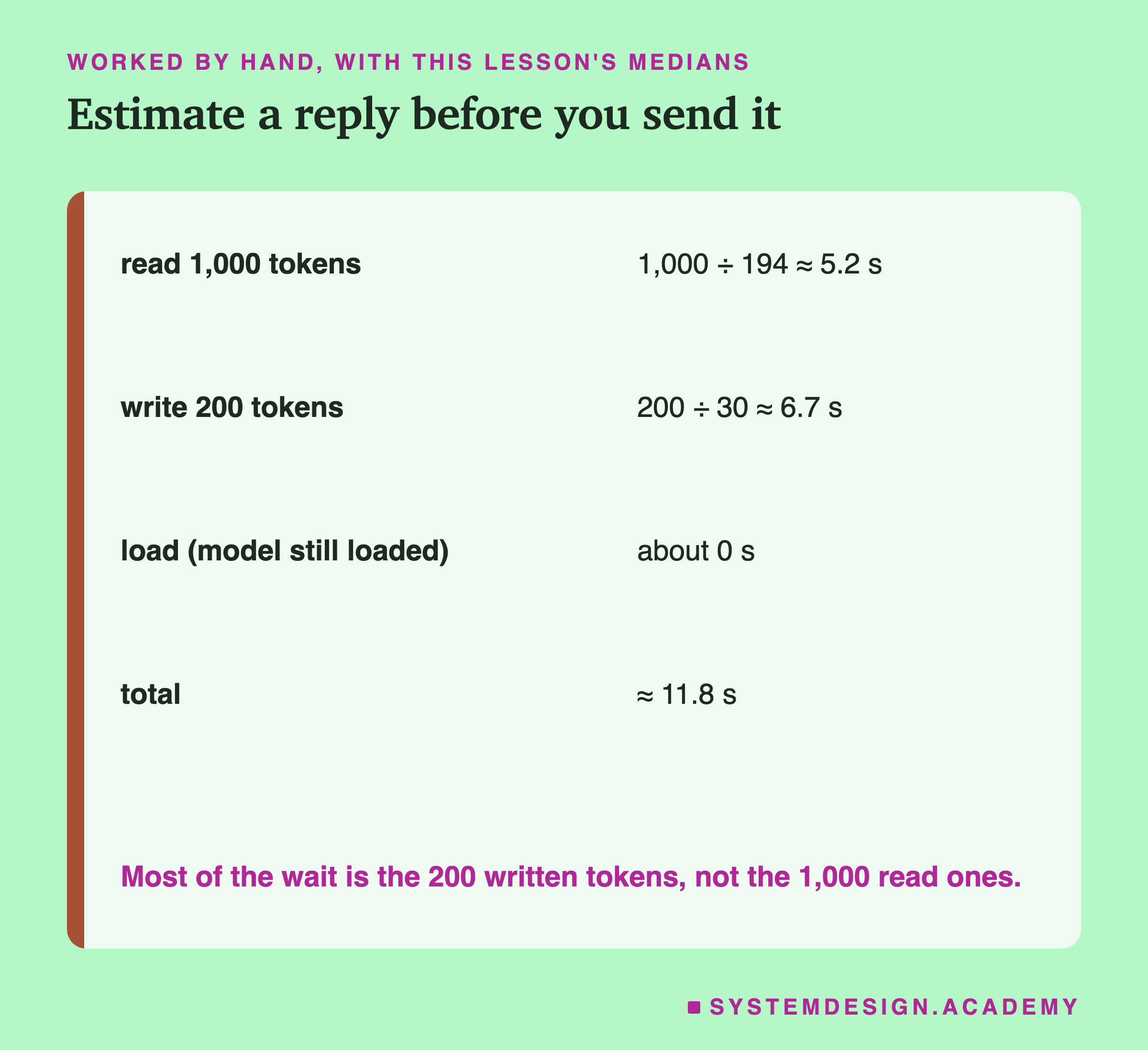
The formula is: time ≈ load + prompt tokens ÷ reading speed + reply tokens ÷ writing speed.

Worked with this lesson's medians, 194 tokens a second for reading and 30 for writing, and a model already in memory: a 1,000-token prompt with a 200-token reply takes about 1,000 ÷ 194 ≈ 5.2 seconds of reading plus 200 ÷ 30 ≈ 6.7 seconds of writing, about 11.8 seconds in all. (The two rounded parts add to 11.9; the total is worked from the unrounded values.)

Now turn it around. A 200-token prompt with a 1,000-token reply: 200 ÷ 194 + 1,000 ÷ 30 ≈ 1.0 + 33.3, about 34.4 seconds once the unrounded parts are added. The two calls handle the same 1,200 tokens in total, but the second one takes about three times as long, only because more of its tokens are written instead of read.

This estimate is rough. The speeds change with prompt length, with the machine and with whatever else is running. But it is good enough to spot a design that will feel slow before you build it.

The estimate also explains a design choice you see in almost every chat app.

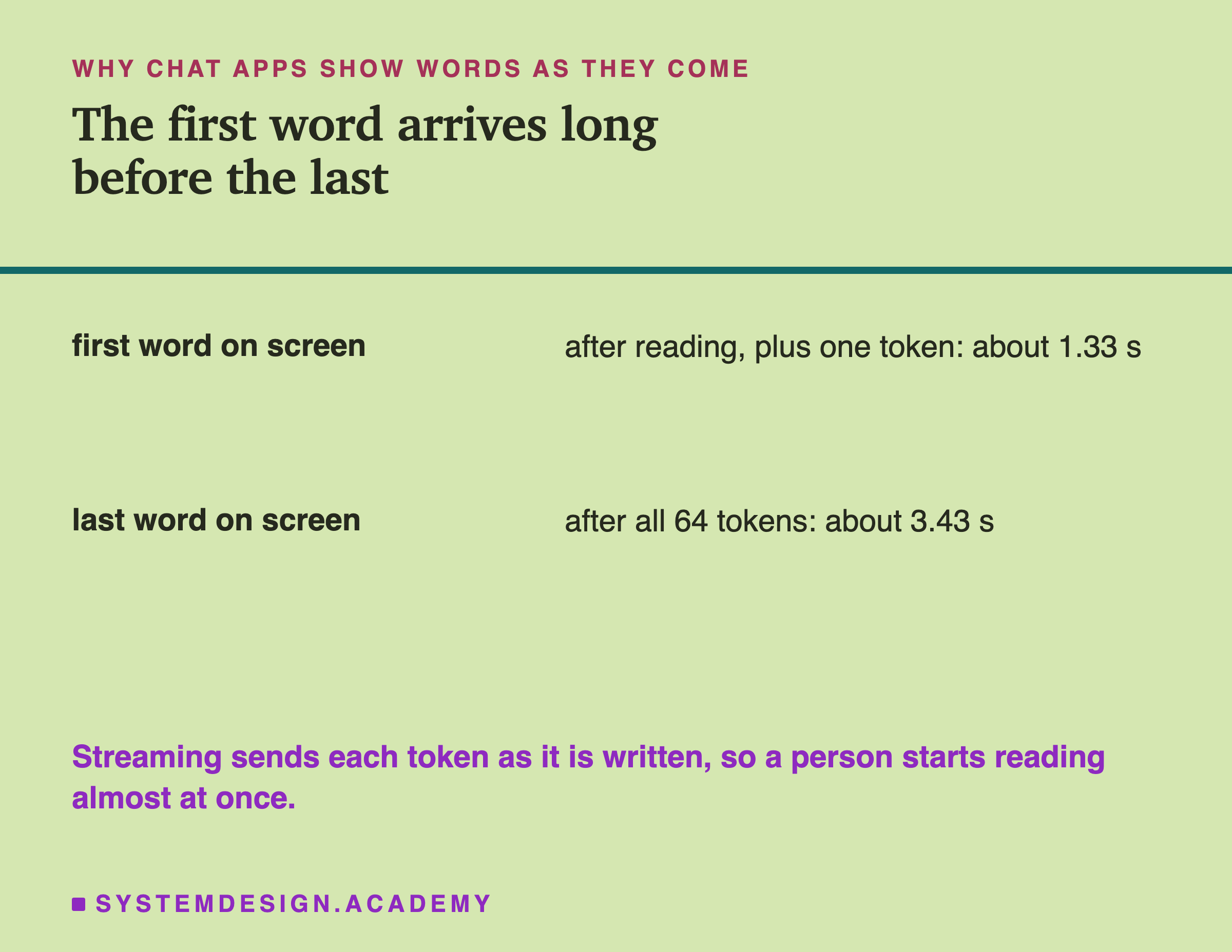
If an app waits for the whole reply before showing anything, the person stares at an empty screen for the full time. For a 256-token prompt and a 64-token reply, that is about 1.30 seconds of reading plus 64 ÷ 30 ≈ 2.1 seconds of writing, about 3.4 seconds in all.

If the app streams, it shows each token the moment it is written. The first word appears after the reading and one written token: about 1.30 + 1 ÷ 30 ≈ 1.33 seconds. The rest arrives while the person is already reading. The total time is the same, but it feels much faster.

In Ollama, streaming is the default. The scripts in this lesson set "stream": false only so that one JSON reply comes back with all the timings in it.

The third part of the wait is loading, and it can be the biggest of all.

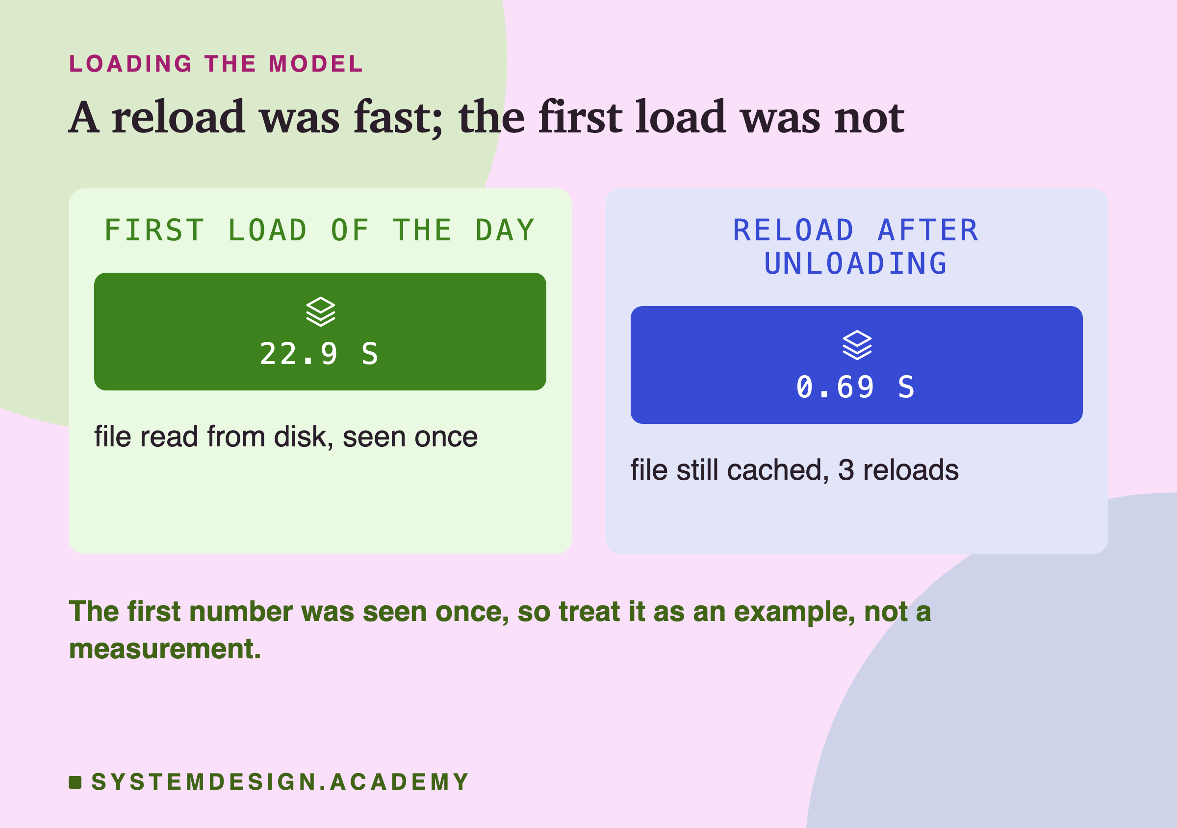
There are three situations, and they are easy to mix up. If Ollama still has the model loaded from a recent call, loading takes about 0 seconds; that is the case in the estimate above. If Ollama has unloaded the model but the laptop's operating system still keeps a copy of the file in memory, a reload is quick: in the lab I unloaded the model three times, and each reload took 0.69 seconds. If the file has to be read from the disk, loading is slow: the very first call I made that day spent 22.94 seconds loading.

I saw the 22.94-second load only once, so treat it as an example, not a measured average. Even so, it shows that the first call can be much slower than the rest. Ollama keeps a model in memory for a while after each call, five minutes by default, so a steady stream of calls stays warm. If your app is quiet for longer, the next person may hit a slow cold start.

The timings are easy to read, but a few details can fool you.

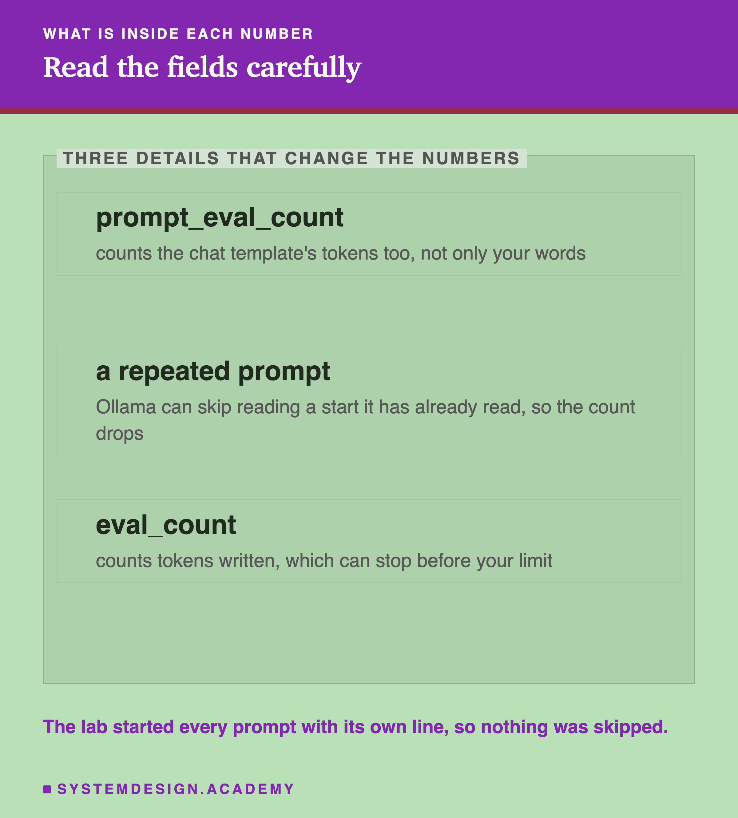
The template counts. prompt_eval_count includes the tokens of the chat template that Ollama wraps around your prompt, not only your own words. My 27-word prompt became 58 tokens.

A repeated start is skipped. If you send the same prompt twice, or two prompts that begin the same way, Ollama can reuse the reading it has already done for the shared start. Then prompt_eval_count drops and reading looks impossibly fast. A later lesson in this chapter covers this cache on purpose; for measuring speed, it is a trap.

The reply can end early. eval_count is the number of tokens actually written. The model may stop before your num_predict limit, as it did at 192 of 256. Always divide by the count, never by the limit you asked for.

This box cannot reach a model, so it holds the timing fields of one real reply, saved from my laptop. It works out the speeds by hand, then uses the lab's medians to estimate three calls.

When you press Run, it prints reading at 398 tokens a second, writing at 45.0, and a ratio of 8.8. Then it estimates 6.8, 11.8 and 34.4 seconds for the three calls. Try changing READ_PER_S and WRITE_PER_S to the numbers from your own run of read_write_speed.py, and see how your machine changes the estimates.

The request. body names the model, the prompt and two options. "num_predict": 64 caps the reply at 64 tokens. "temperature": 0 makes the pick greedy, as lesson 2 explained, so the same prompt gives the same reply and the timing is easier to compare. "stream": false asks for one JSON answer instead of a stream of pieces.

The call. urllib.request.Request builds an HTTP POST to Ollama on localhost:11434, the port Ollama listens on. urlopen sends it and waits. json.loads turns the answer into a Python dictionary.

The conversion. Each ..._duration field is divided by 1e9, which is Python's way of writing one billion, to turn nanoseconds into seconds.

The speeds. read_n / read_s and write_n / write_s are the two speeds in tokens a second. That division is the whole measurement.

The lab. speed.py does the same thing 35 times. Its measure function builds the list of settings, shuffles it with (a random order that is the same every time, because the seed, 7, is fixed), and calls Ollama once per setting with mode and a of 8,192. is the size of the model's working window in tokens, set large enough for the longest prompt. Its function prints medians and ranges, and computes the "slowest reading against fastest writing" check directly from the saved calls, so that line cannot be typed by hand.

Timing the whole request and calling it "model speed". Total time mixes loading, reading and writing. Split it using the fields, or you will not know which part to fix.

Dividing by the limit instead of the count. If you asked for 256 tokens and the model wrote 192, divide by 192.

Measuring once. One call on a laptop can be far off. The same setting in this lab ranged from 22 to 42 tokens a second for writing.

Measuring in blocks. Running one setting after another can make drift look like a difference between settings. Shuffle the order.

Repeating the same prompt. Ollama may skip reading a start it has seen, and reading then looks impossibly fast. Give each timed prompt its own start.

Including the first call. The first call may include a cold load of many seconds. Warm the model up with one call you do not count, as the lab did.

Blaming the prompt for a slow app. On this laptop a 1,000-token prompt took about 4.4 seconds to read, while a 192-token reply took 6.4 seconds to write. Check the reply length first.

When speed matters, look at the reply first. Ask for shorter answers, set num_predict, and ask for a list or a short sentence when that is all you need.

Stream whenever a person is waiting. The total does not change, but the first word arrives in about the time it takes to read the prompt.

Keep the model warm for steady traffic. Ollama's keep_alive option controls how long a model stays in memory after a call. Longer means fewer cold starts, at the cost of memory held while idle.

Do not over-trim the prompt. Cutting a 1,000-token prompt to 500 saves about 2.5 seconds at this laptop's reading speed, but it may remove the very context the answer needs. Trim the reply first.

When not to rely on these numbers. They come from one small model on one busy laptop. A server with a big graphics card, many people calling at once, or a much larger model will all change them. Measure on the machine you will actually use, with the method from this lesson.

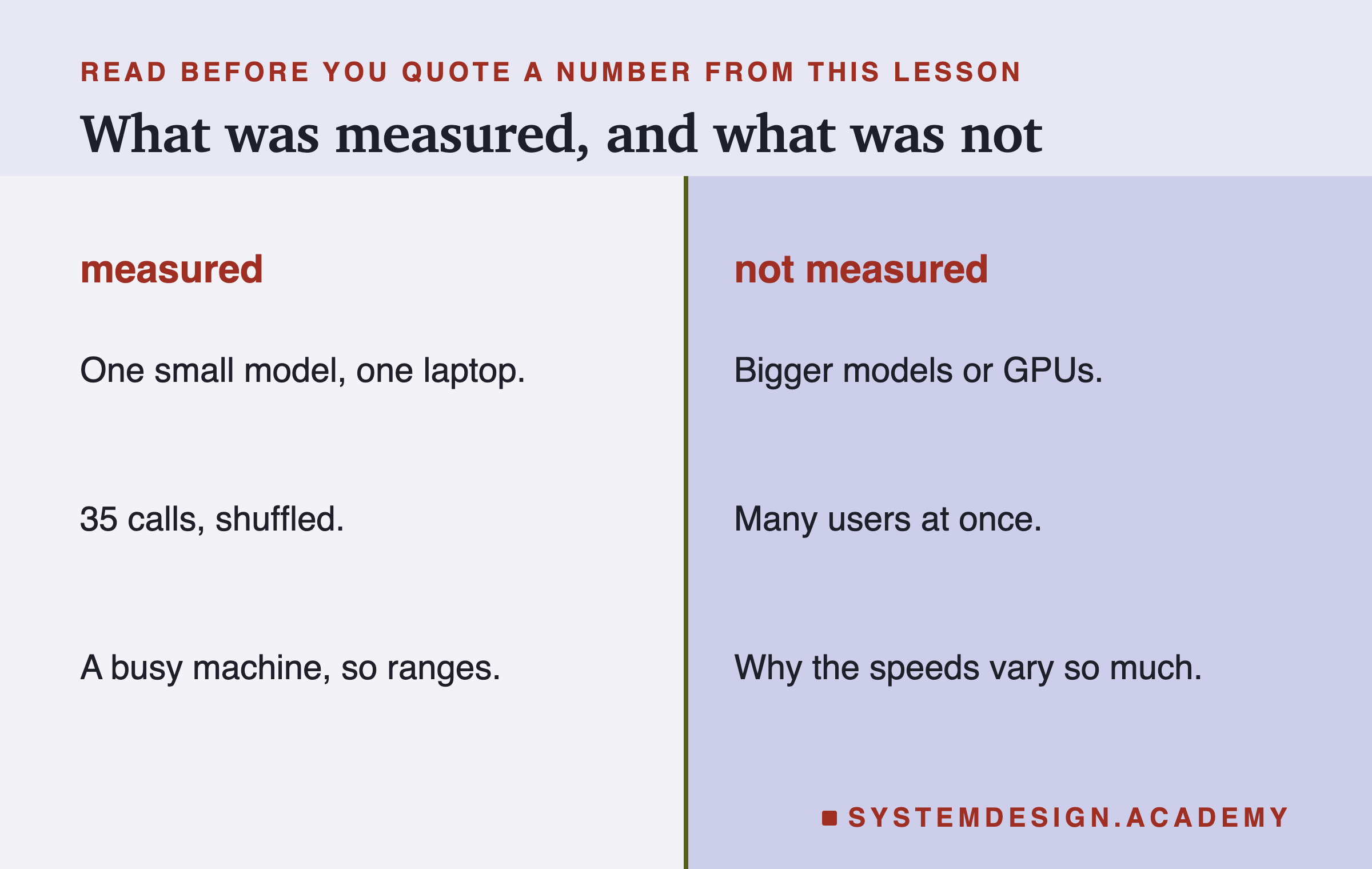
The lab measured one model, qwen2.5:3b, on one laptop, over 35 calls in a shuffled order, on a machine that was busy with other work. That is enough to show the direction clearly, reading much faster than writing, and to show how times grow with prompt and reply length.

It did not test bigger models, dedicated graphics cards, or many people using the same model at once. On a shared server, several requests can be written in the same pass, which changes the picture a lot. It also could not explain why the laptop slowed down during the run.

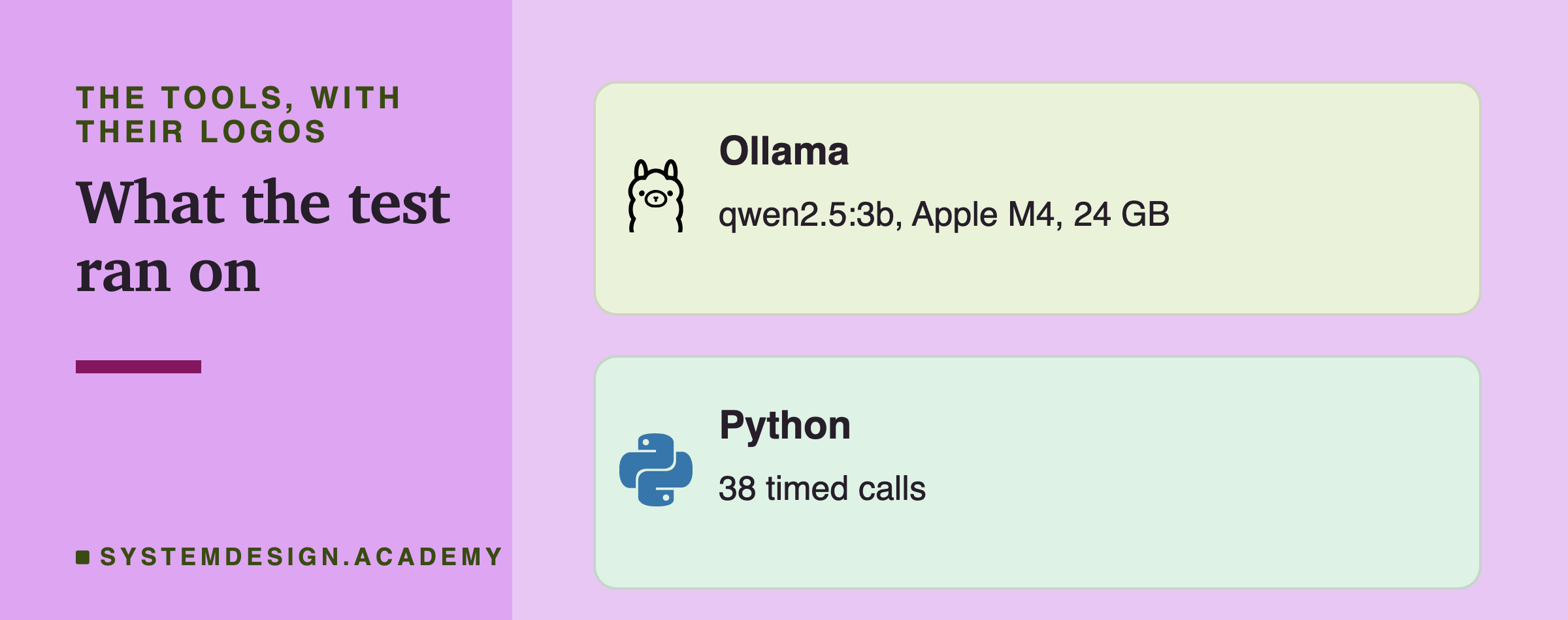
Everything ran locally with free tools, Ollama and Python: the 35 lab calls and 3 reloads, 38 timed calls in all. You can repeat the whole thing on your own machine without an account or a bill.

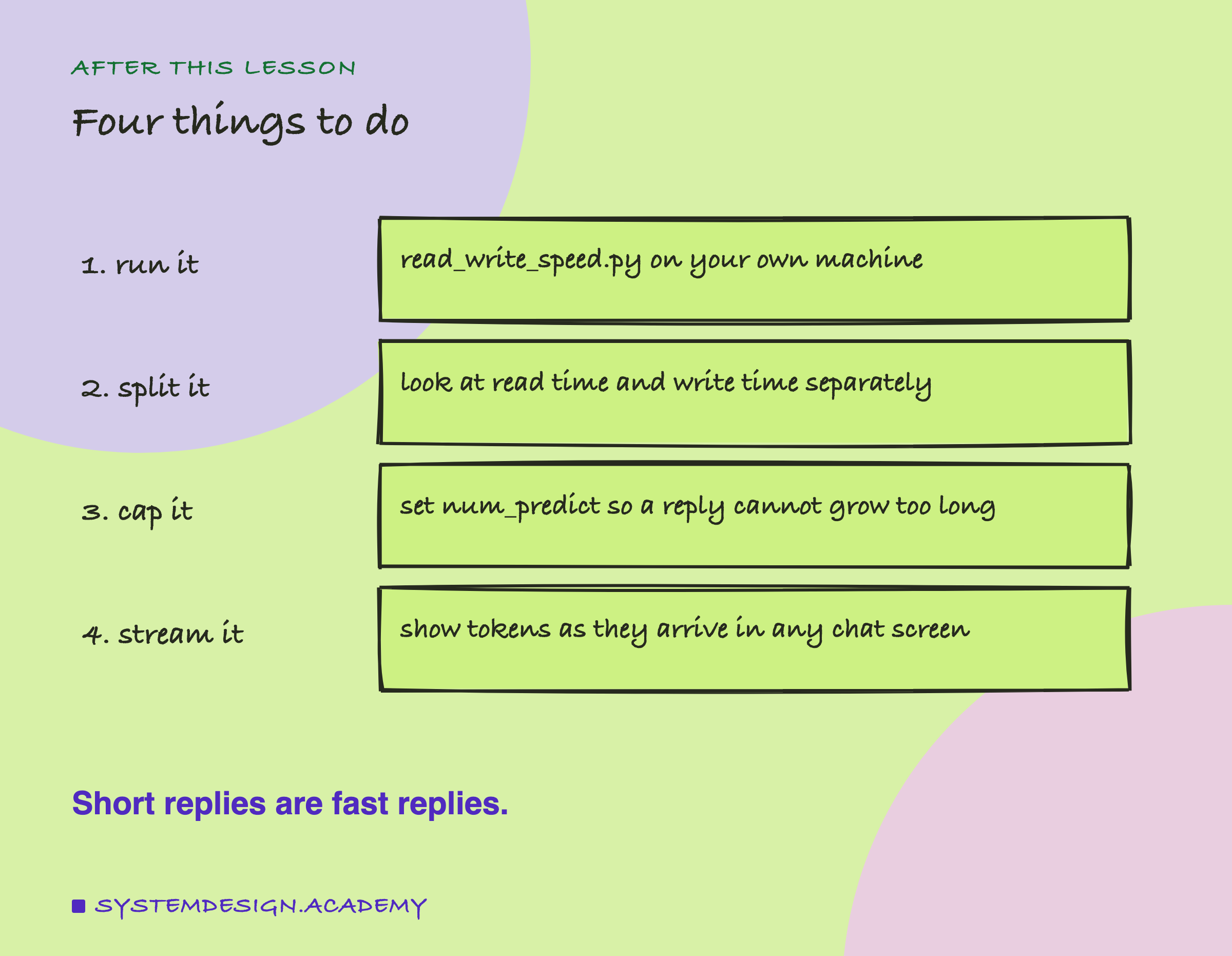
Run read_write_speed.py on your own machine and write down your two speeds. Then look at one real call in your own app and split its time into load, read and write. In most apps, the biggest part will be the writing, and the cheapest fix is a shorter reply or a streamed one.

The next lessons in this chapter go inside the reading step: what attention is, what a long prompt really costs, and how a cache lets a model skip reading what it has already read.