A Practice Test Made From the Real Exam
Let me start with a picture.
A teacher wants to know if the class is ready for the final exam. So she writes a practice test. But she writes it with the real exam paper open beside her, and copies some of its questions.
The class does well on the practice test. Is the class ready? We cannot tell. The practice test was not a fair preview of exam day, because the exam leaked into it.

Machine learning has the same trap. It is called leakage. The data you test on is supposed to stand in for new data the model has never seen. If anything learned from the test data slips into training, the test score stops meaning anything.
Everyone knows the rule "split first". What is less known is that the leak often hides in a small preparation step that runs before the split, and looks harmless. This lesson measures four of those steps. Some of them lie badly. One barely matters.
The Words You Need First
Please read this slide slowly if any word is new. Every slide after it uses these words.
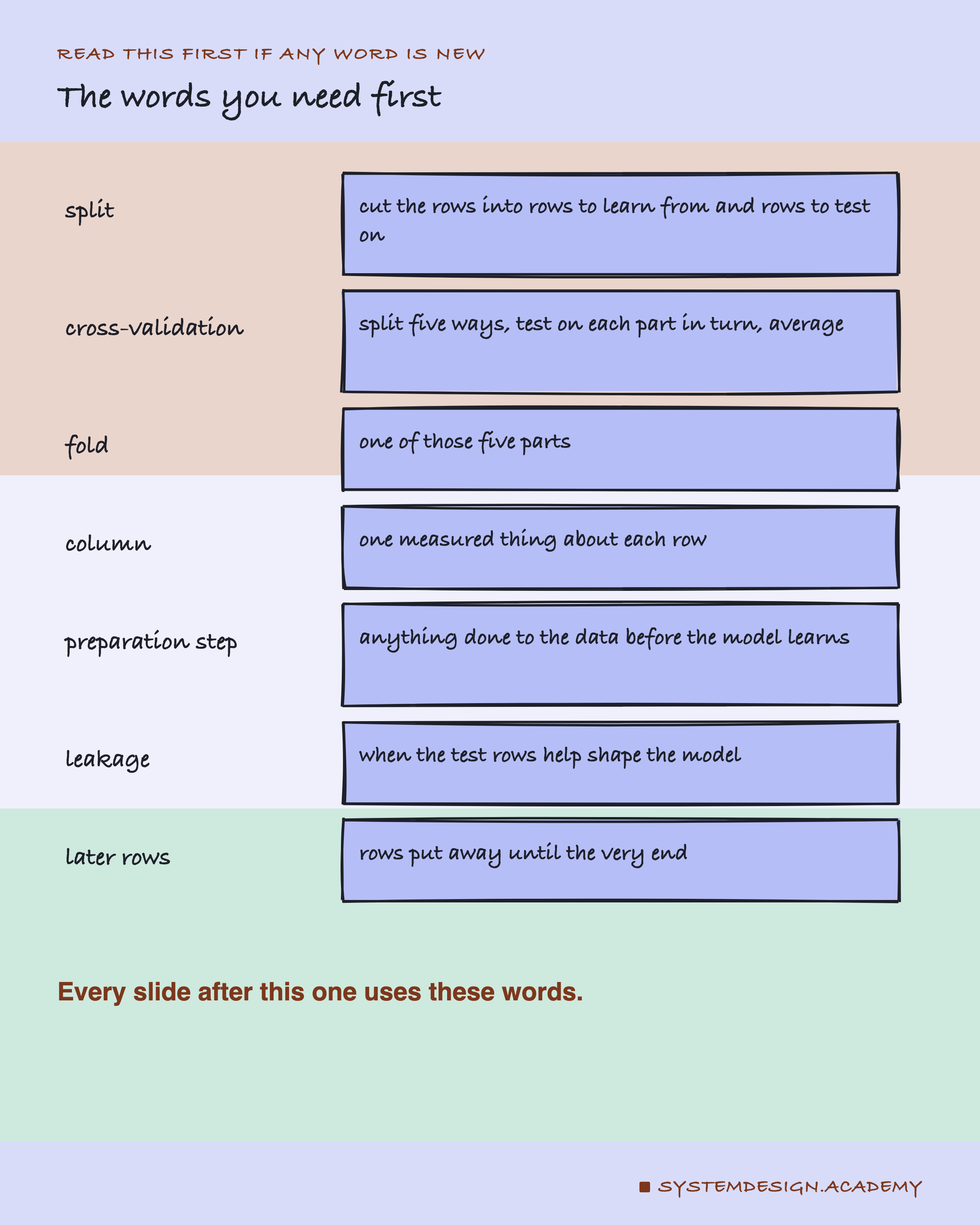
Row and column. A dataset is a table. Each row is one example, like one patient. Each column is one thing measured about it, like tumour size.
Label. The answer we want the model to learn, like "malignant" (cancerous) or "not".
Split. Cutting the rows into a part the model learns from and a part it is tested on.
Cross-validation. Splitting the rows into parts called folds, often five. Each fold takes a turn as the test part while the model learns from the others, which I call the learning rows. Those test parts are the test rows. The test scores are averaged. That average is an estimate: a guess, made before launch, of how well the model will do on new data.
Preparation step. Anything done to the data before the model learns: choosing which columns to keep, rescaling numbers, filling gaps, copying rare rows.
Leakage. When the rows used to test a model help shape it. The test score then promises more than new data will give.
Later rows. Rows put away at the very start and not touched until the end. Other books call them the test set or the holdout set. The rest of the rows, used for everything else, I call the building rows.
Seed. A number that fixes one random cut of the data, so a run can be repeated exactly.
Two Recipes, One Difference
Here are the two recipes this lesson compares. They use the same data, the same step and the same model. Only the order changes.
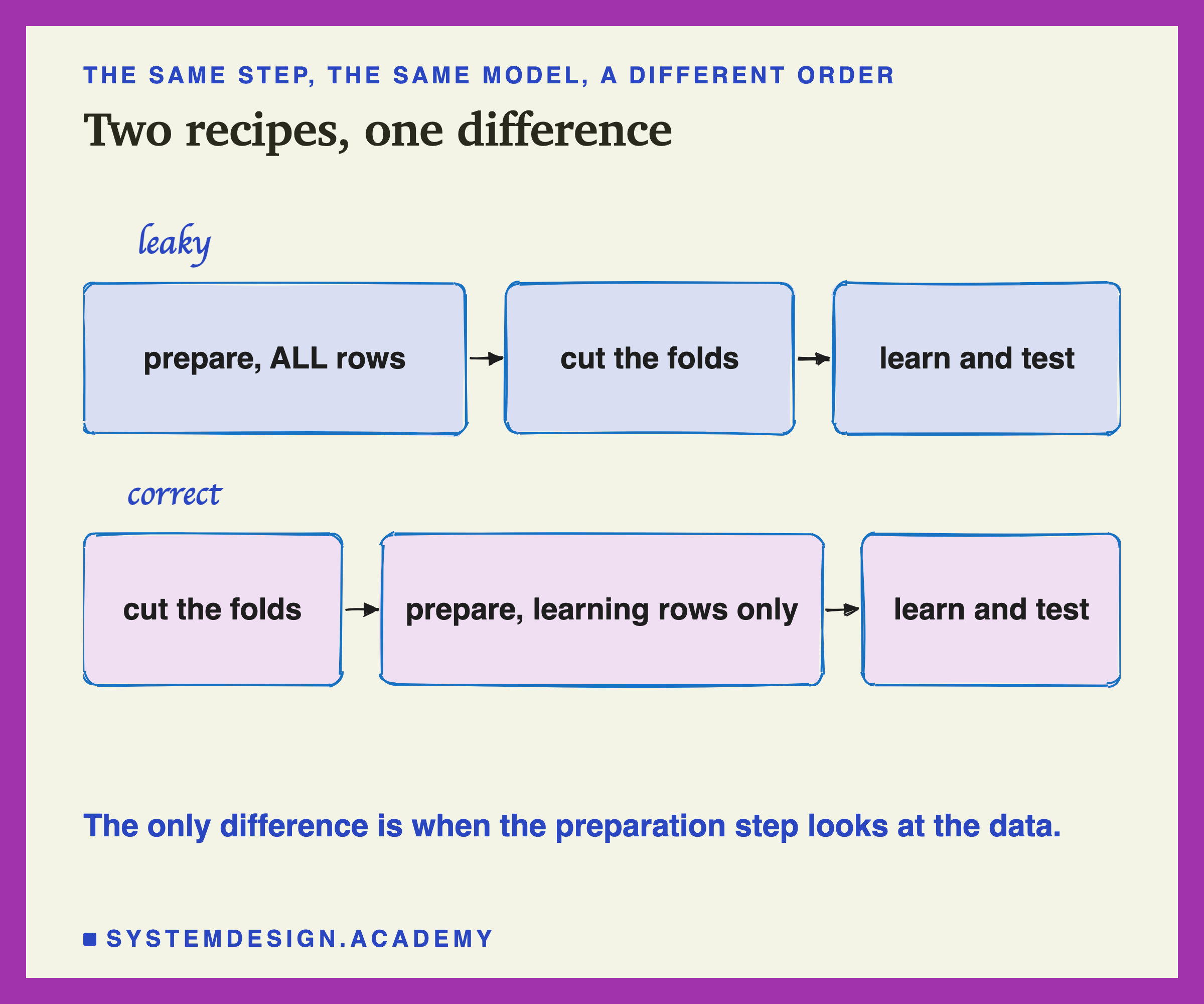
Leaky. Run the preparation step on all the rows first. Then cut the folds and cross-validate. The step has already looked at the rows that will later be used for testing.
Correct. Cut the folds first. Inside each fold, run the preparation step on the learning rows only, then apply what it learned to the test rows.
The leaky recipe is shorter to write, and it is what many notebooks do by accident. The question is how much it matters.
How the Lab Was Built
-
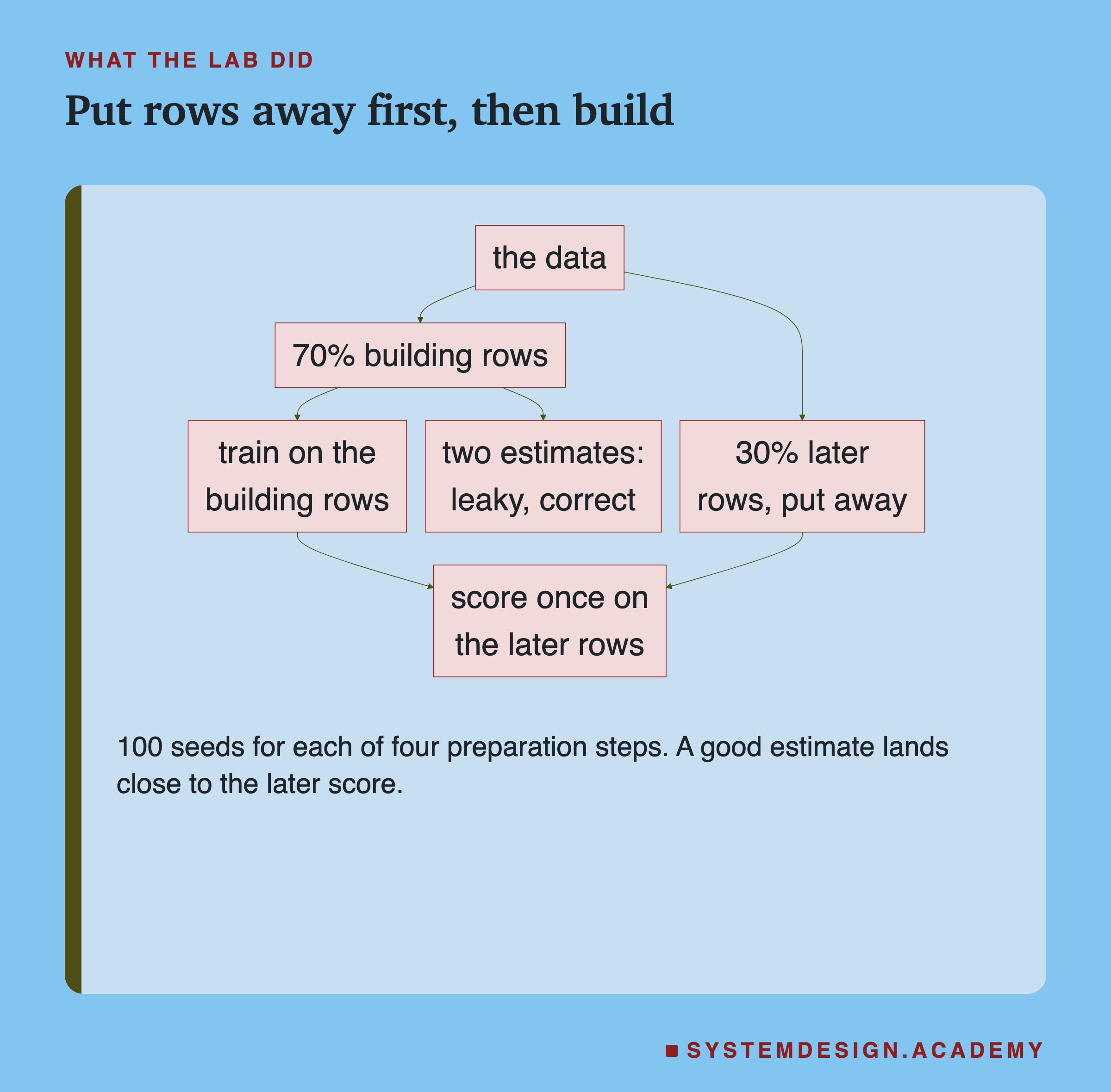
Put some rows away. Before anything else, 30% of the rows are put away and not touched. I call them the later rows. They stand in for the new data the model meets after launch.
-
Two estimates. On the other 70%, the lab cross-validates twice: once with the leaky recipe, once with the correct one.
-
The truth. Then it trains the recipe once on all of the 70%, and scores it once on the later rows. That is what you would actually get.
-
Repeat. All of that runs 100 times per step, with a different random cut each time. A seed is the number that fixes one random cut, so each run can be repeated exactly.
A good estimate lands close to the later score. The lab asks which estimate does.
The Four Preparation Steps
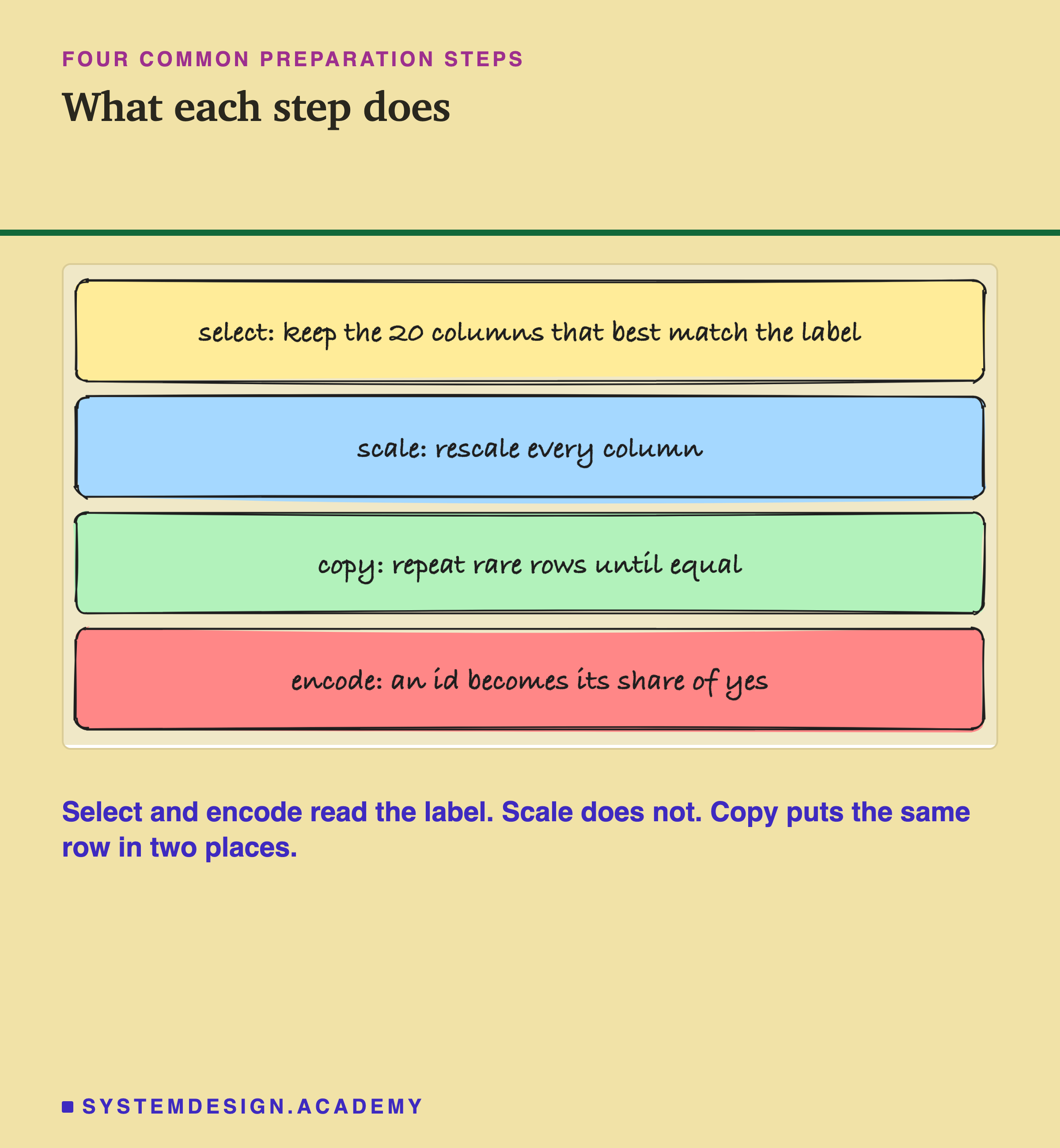
1. Select columns. Keep the 20 columns that best match the label, out of many.
2. Scale columns. Rescale every column so its average is 0 and its values usually sit within about 1 of that average.
3. Copy rare rows. When one kind of row is rare, copy those rows until there are as many as the rest.
4. Encode an id. Replace an id, like a customer number, with the share of "yes" answers among that id's rows. This is called target encoding.
Two of the steps run on pure noise, random numbers where nothing can be learned, so the honest score is known: 0.5, a coin flip. The other two run on real breast tumour data. Each step's own slide says which data and which model.
What Each Estimate Promised
| step | score | leaky | correct | later |
|---|---|---|---|---|
| select, on noise | accuracy | 0.927 | 0.495 | 0.498 |
| scale, on tumours | accuracy | 0.962 | 0.962 | 0.963 |
| copy, on tumours | F1 | 0.996 | 0.867 | 0.876 |
| encode, on noise | accuracy | 0.792 | 0.497 | 0.501 |
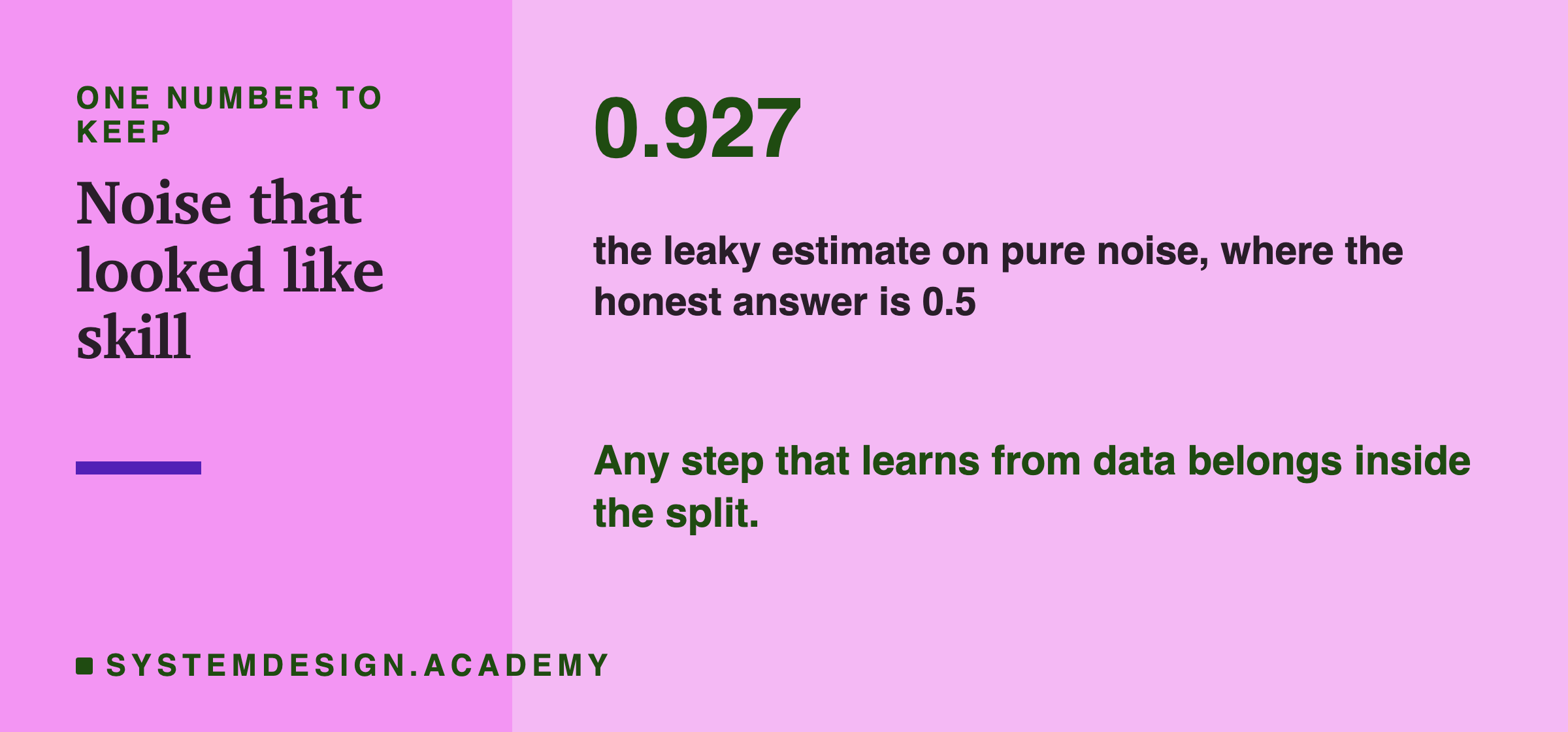
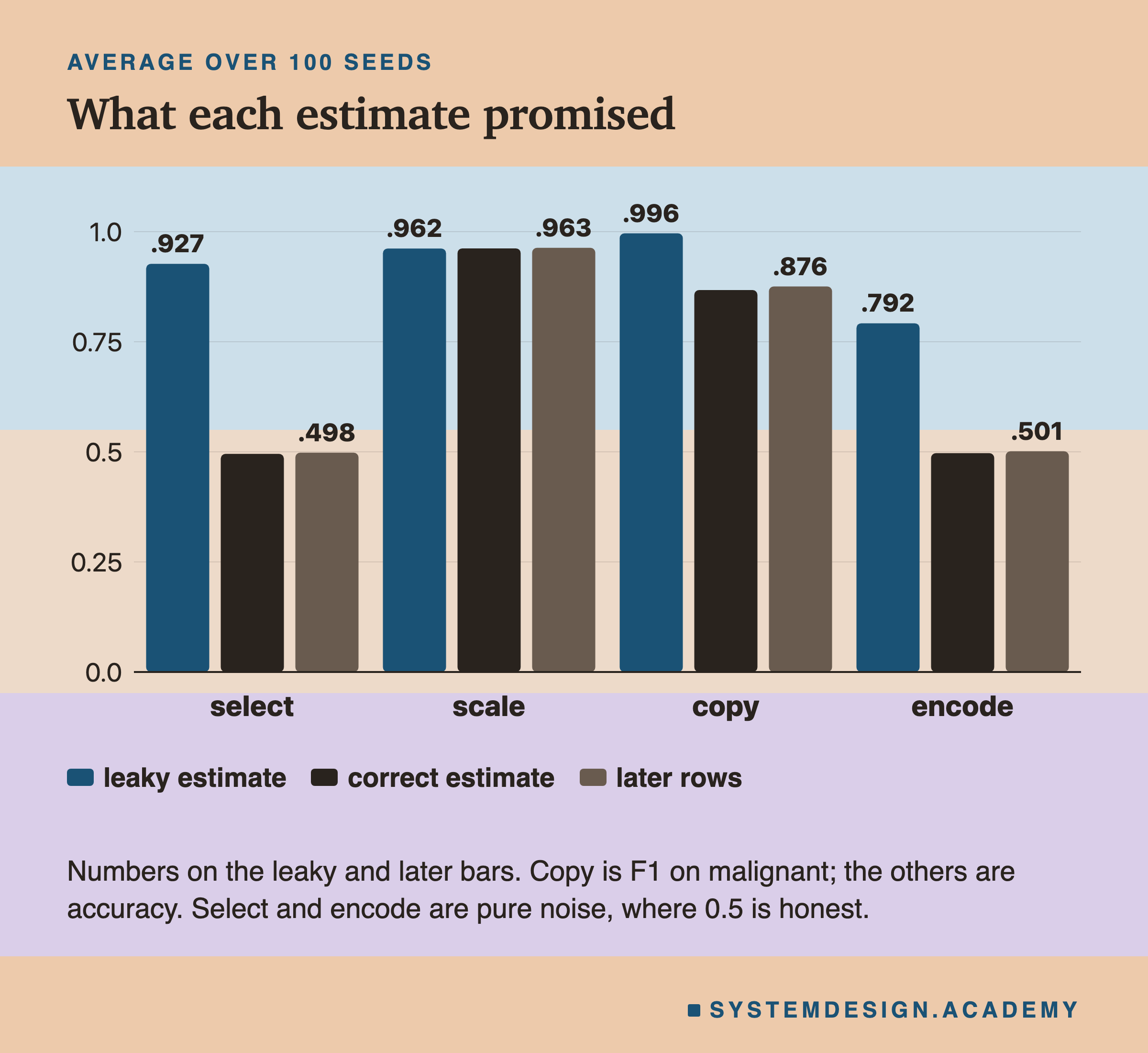
Each number is the average over 100 seeds. Accuracy is the share of rows labelled right. F1 is a score for a rare class, high only when the model finds most of the rare rows and is mostly right when it says "rare". Both run from 0 to 1. Three of the four leaky estimates promised far more than the later rows gave. On pure noise, choosing columns before the split promised 0.927 and delivered 0.498. Target encoding promised 0.792 and delivered 0.501. Copying rare rows promised an F1 of 0.996, nearly perfect, and delivered 0.876.
The Lab, Running
This is a real recording of the lab's report, printed on the laptop where the lab ran.
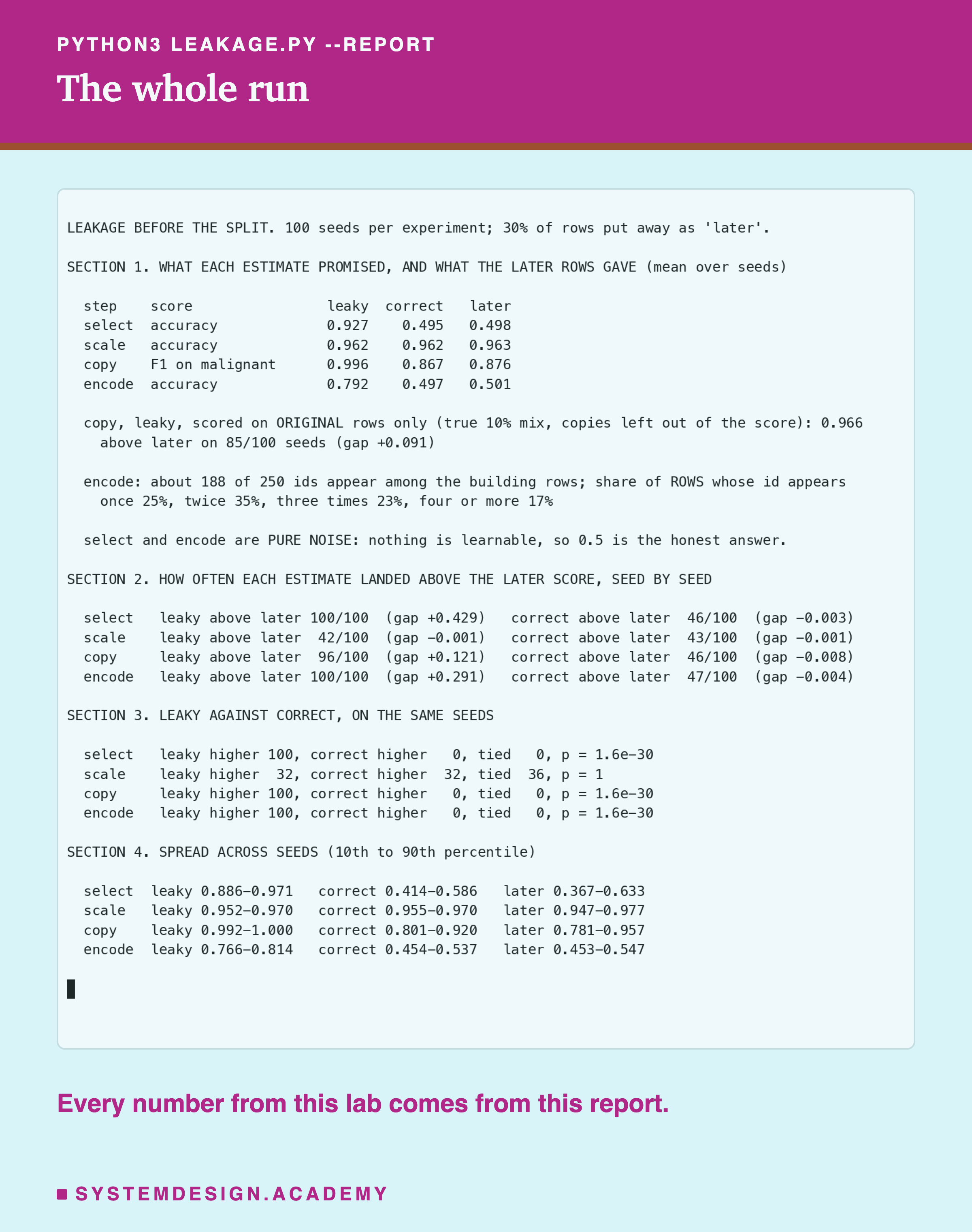
In the recording, "leaky" and "correct" are the two cross-validation estimates, and "later" is the score on the rows put away at the start. "gap" is an estimate minus the later score: above 0 means the estimate promised too much. "p" says how rarely a split this uneven would happen by luck; "1.6e-30" is far less than once in a million. "10th to 90th percentile" means the range that holds the middle 80% of the seeds, leaving out the lowest tenth and the highest tenth.
The next four slides take each step in turn and show where the false promise came from.
How Pure Noise Scored 93 Percent
The data. 100 rows of pure noise: 5,000 columns of random numbers and a random yes or no label. 30 rows are put away as later rows, which leaves 70 building rows. The model is logistic regression, a simple model that gives each column a weight, a number for how much it counts, and adds them up.
The select step ran on pure noise, where a coin flip is the honest score. The leaky estimate said 0.927: the model seemed to be right about 93 times in 100. On the later rows it scored 0.498. The correct estimate said 0.495.
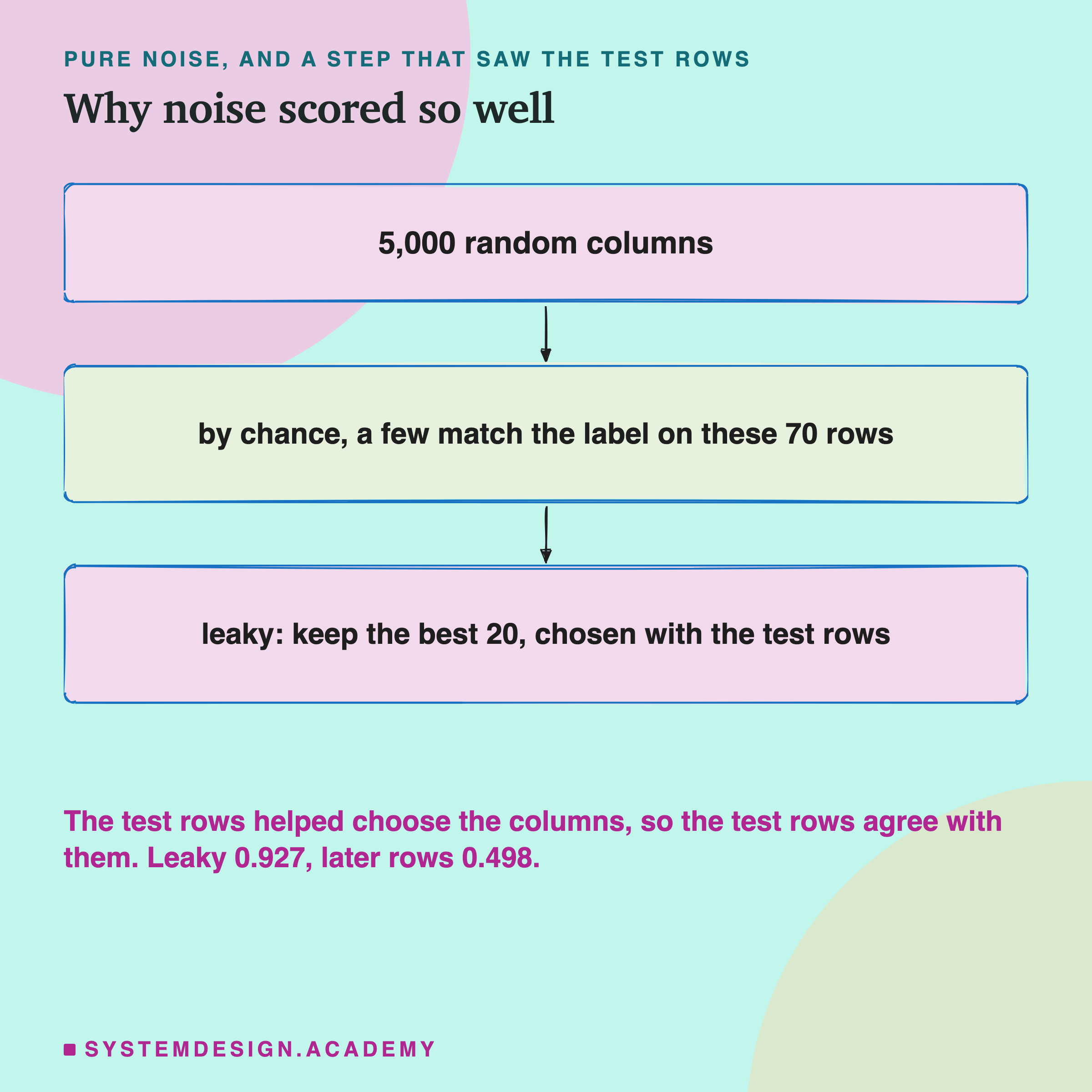
Here is why. With 5,000 random columns and only 70 building rows, some columns will line up with the label just by chance. Flip 5,000 coins 70 times each, and a few of them will match your yes and no answers far better than half the time, purely by luck. The leaky step looks at all 70 rows and keeps the 20 that line up best.
But those rows include every row that will later sit in a test fold. So the columns were chosen partly because they happen to agree with the test rows. Of course the model then scores well on them. It is the practice test copied from the exam.
The correct recipe chooses columns using the learning rows only. The lucky columns it finds are lucky only on those rows. On the test fold they are ordinary noise again, and the score falls back to a coin flip, where it belongs.
Not Once, Every Time
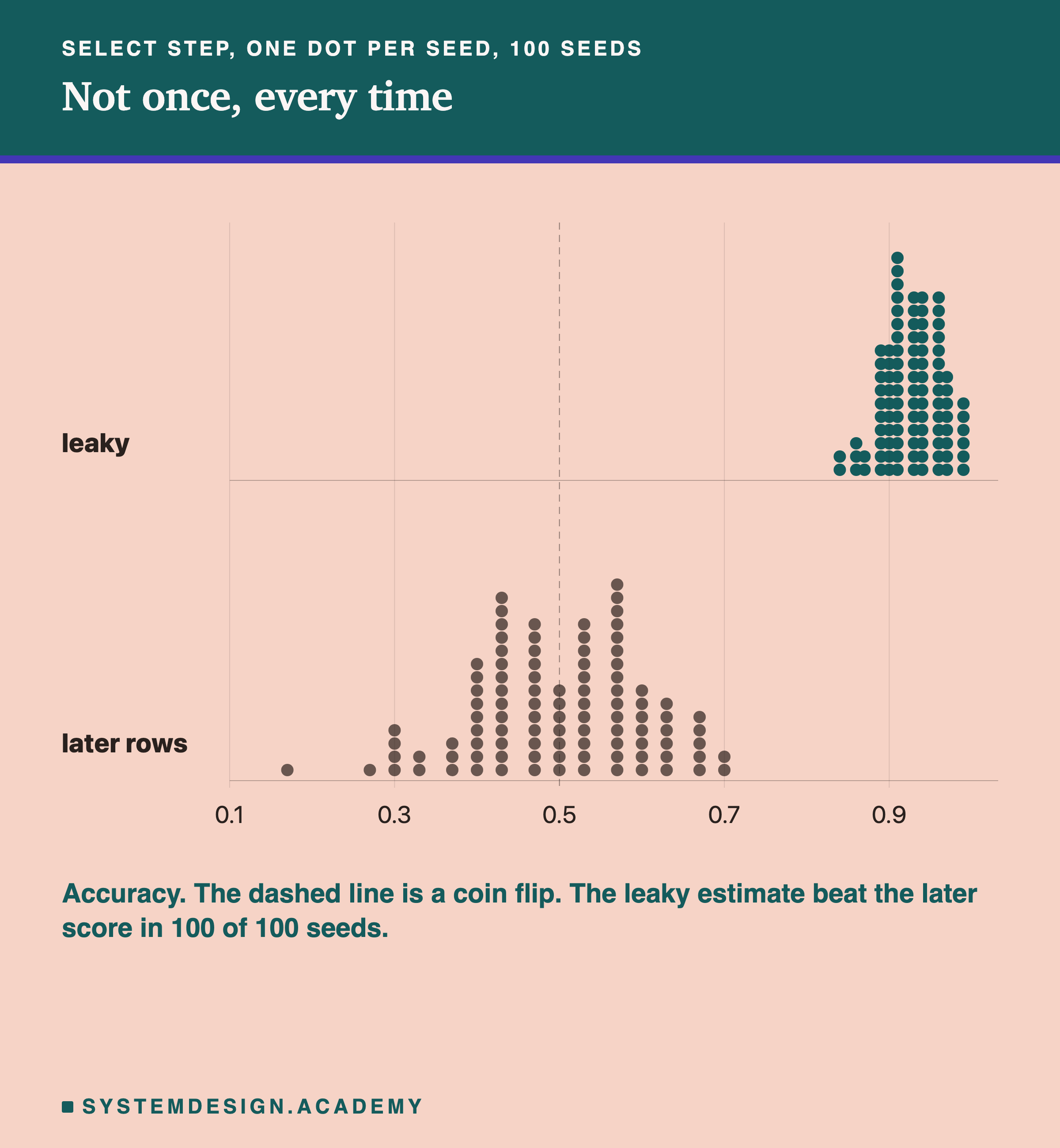
An average can hide a few wild seeds, so here is every seed.
For the select step, the leaky estimate was above the later score in 100 of 100 seeds. In the middle 80% of seeds it ran from 0.886 to 0.971. The middle 80% of later scores ran from 0.367 to 0.633, spread around a coin flip, because 30 later rows is a small test.
The correct estimate was above the later score in 46 seeds and below it in 52, and tied with it in 2. The figure shows only the leaky and later rows; the correct estimates look like the later ones. That is what an honest estimate looks like: sometimes a little high, sometimes a little low, right on average.
Comparing the two estimates seed by seed, leaky beat correct in 100 of 100. If the two recipes were equally good, each would win about half the seeds, like coin flips. A split this uneven happens by luck less than once in a million tries.
The Id That Knew the Answer
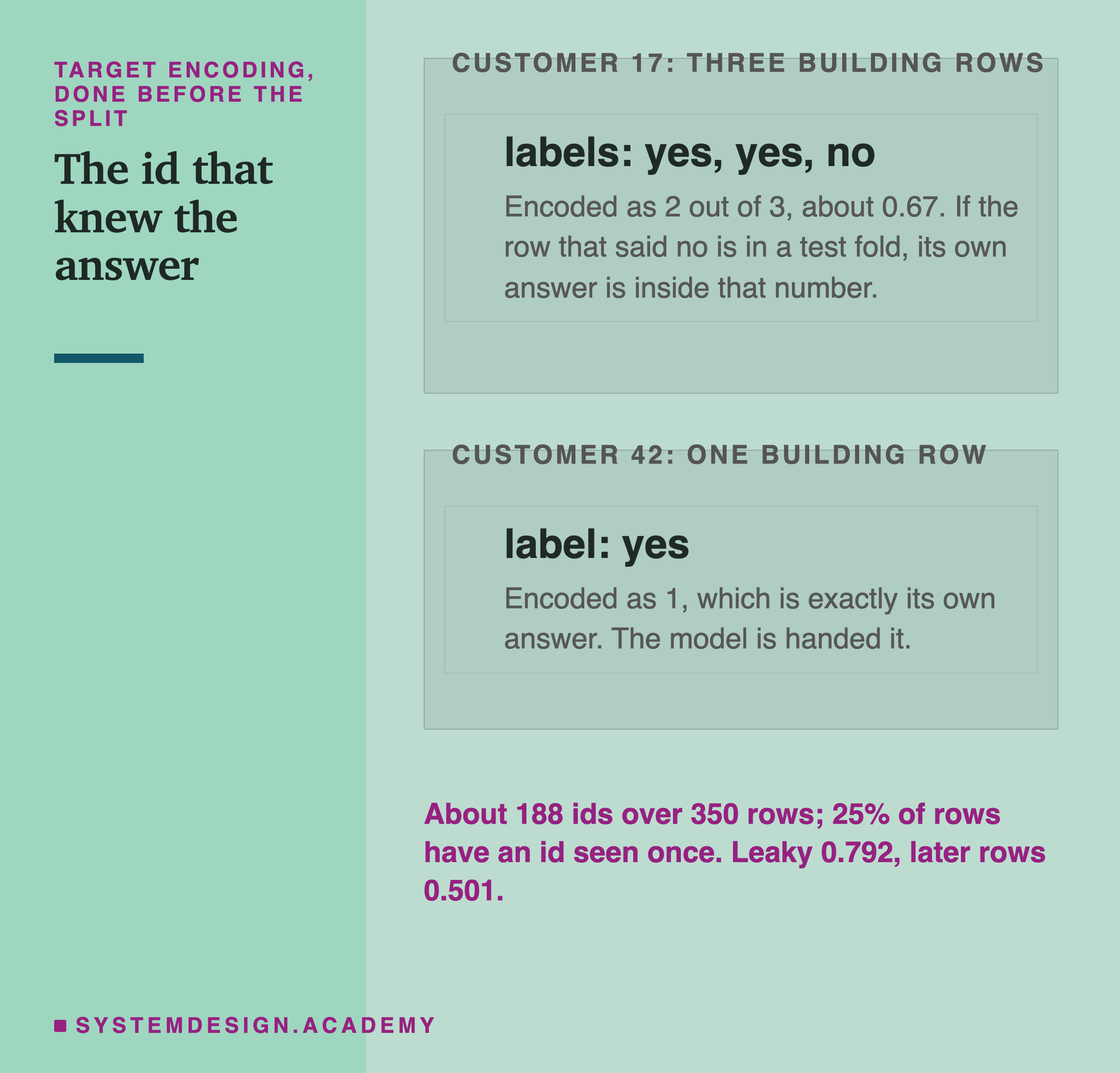
The data. 500 rows of pure noise, each with a random customer id out of 250, and a random yes or no label. The model is logistic regression again, with the encoded id as its only column.
Target encoding also ran on pure noise. The leaky estimate said 0.792. The later rows gave 0.501.
Here is why. About 188 of the 250 ids turn up among the 350 building rows, so each id has only a few rows. 25% of the rows have an id seen only once. That id's encoding is the share of yes among that one row: 1 if the row's label is yes, 0 if it is no. The model is handed the answer.
The other rows leak too, just less. An id seen two or three times still counts the row's own label inside its share, which pulls the share toward the right answer.
Done the leaky way, the encoding is worked out before the folds are cut, so a test row's own label is inside its own encoding. For an id with three rows, yes, yes and no, the encoding 0.67 was worked out from all three labels, including the test row's own answer. Done the correct way, the encoding comes from the learning rows only. A test row's id then brings only what other rows said about that id. On noise, other rows tell it nothing about this row, and the estimate falls to 0.497.
The Full Fix for Target Encoding
That makes the estimate honest, but it is not the whole fix. During training, a learning row whose id appears once still gets its own answer as its encoding, so the model learns to trust the id too much.
In practice, use TargetEncoder from scikit-learn, the most common Python library for this kind of model. When it learns, it works out each learning row's encoding from the other learning rows, and it pulls rare ids toward the overall average.
One warning. Its fit_transform call, which learns the encodings and applies them in one go, is the safe one. Learning the encodings in one call and then encoding the same training rows in a second call brings the leak back.
This leak is common in real work, because target encoding is a popular trick for columns like customer, shop or postcode.
Copies on Both Sides of the Line
The data. The 569 real breast tumours, with malignant cut down to 10% of the rows. The model is a random forest: many small decision trees, each a chain of yes-or-no questions about the columns, voting on the answer. The score is F1 on malignant: high only when the model finds most malignant rows and is mostly right when it says "malignant". It runs from 0 to 1.
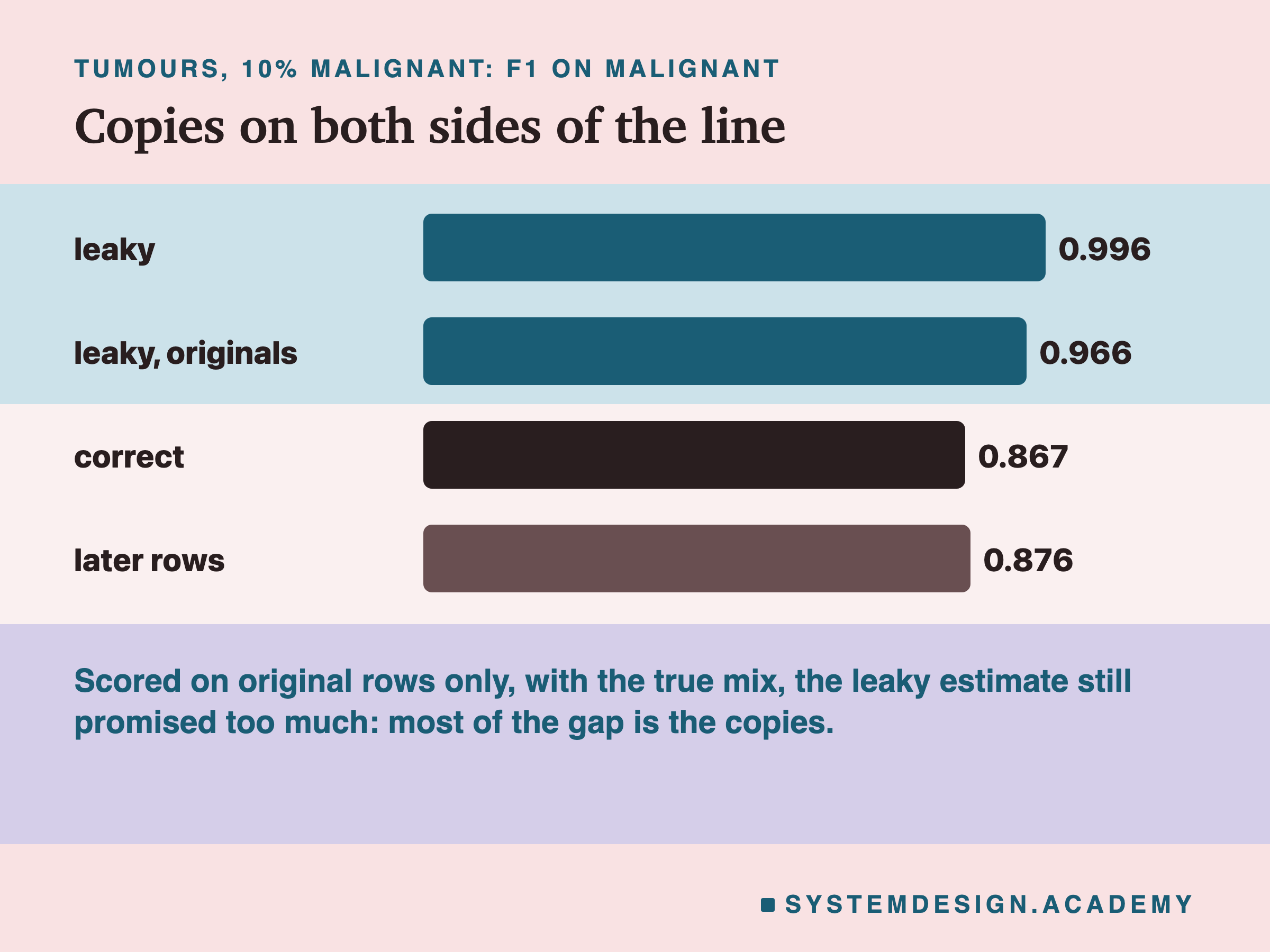
This step used real tumours, with malignant cut to 10% of the rows: about 28 malignant rows among 277 building rows. The leaky estimate was an F1 of 0.996, almost perfect. The later rows gave 0.876.
Copying before the folds are cut puts a malignant row in the learning part and its exact copy in the test part. A random forest has little trouble recognising a row it has already seen.
You might wonder if the high score is only because the test folds now hold more rare rows. That effect is real, but it is the smaller one. After copying, the test folds are about half malignant instead of 10%. F1 is easier to score then. When half the test rows are malignant, a model that says "malignant" often is right more often. To separate the two, the lab also scored the leaky model on the original rows only, which keeps the true mix. That still gave 0.966. So most of the false promise came from the copies, not from the mix.
The correct recipe copies only inside each learning part. It estimated 0.867, close to the later 0.876. It is the same copying step as lesson 108, the one before this, where it was done this correct way.
The same leak happens with no copying step at all when the raw data already holds duplicate rows. Remove exact duplicates, or keep them together on one side, before you split.
The Leak That Barely Mattered
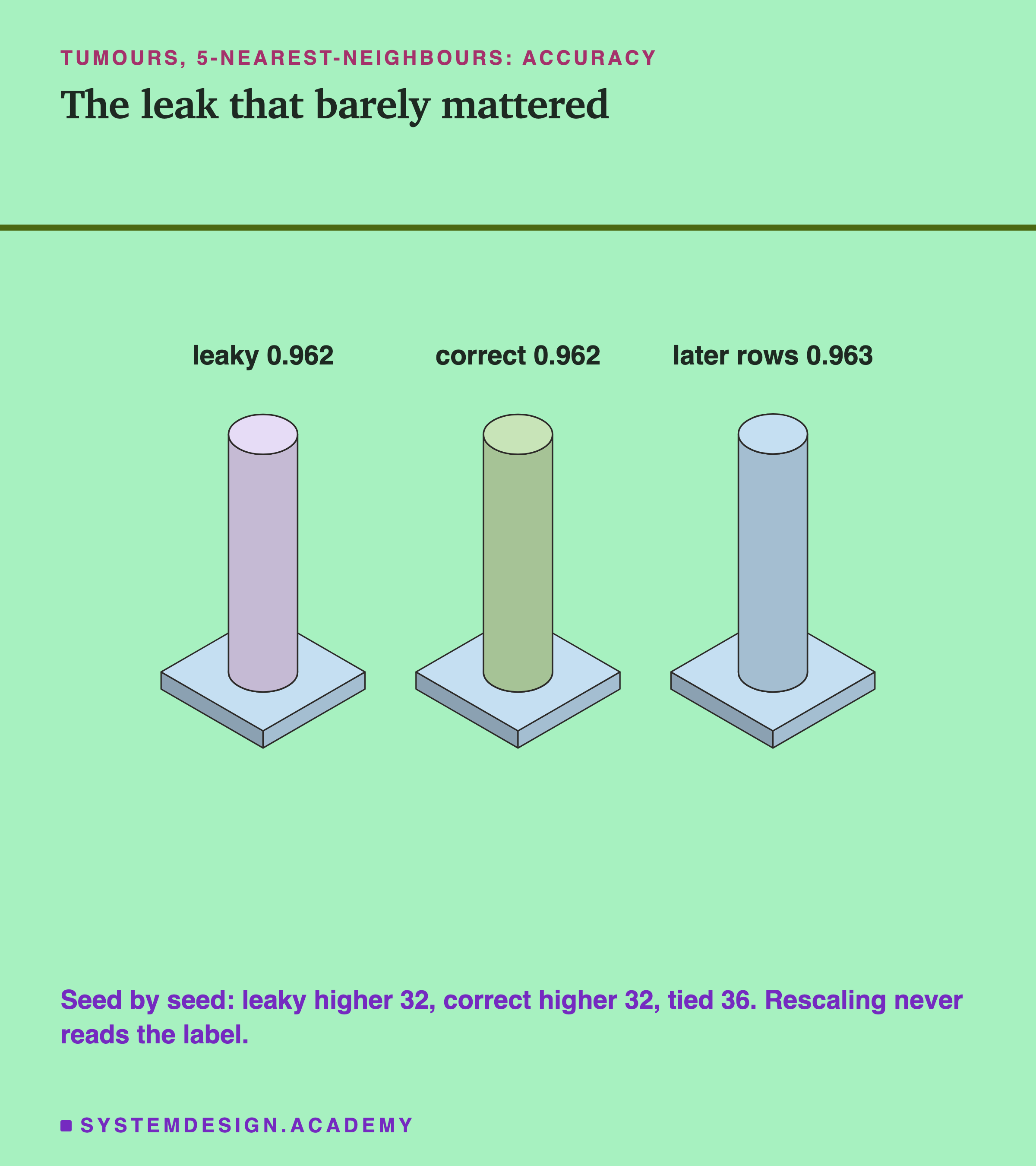
The data. 569 real breast tumours with 30 measurements each. The model is 5-nearest-neighbours: it labels a row by looking at the 5 most similar rows, so it depends heavily on how each column is scaled. The score is accuracy, the share of rows labelled right.
Rescaling leaked too, strictly speaking. The leaky version worked out each column's average and spread using rows that later sat in test folds.
But the estimates were almost the same: 0.962 leaky, 0.962 correct, 0.963 on the later rows. Seed by seed, leaky was higher in 32, correct was higher in 32, and they tied in 36.
Why so small? The average of a column over the 398 building rows hardly moves when one fold is left out, and rescaling never looks at the label. Nothing about the test rows' answers gets in.
So leaks are not all equal. The ones that hurt most read the label, like choosing columns by how well they match it, or target encoding. Or they put the same row on both sides of the line, like copying.
Still put scaling inside the split. It costs nothing, and with fewer rows, leaving one fold out moves the average and spread more, so the leak grows. Other steps that do not read the label can leak more too. Filling gaps, or squeezing many columns into a few, can leak when there are few rows. So can any step on data that changes over time, where the averages would include future rows.
Check the Promise Yourself
This box holds the lab's real results, seed by seed, for two of the steps: select and copy. For each seed there are three numbers: the leaky estimate, the correct estimate and the later score. Press Run to see how far each estimate landed from the later score.
Then find the line that starts with STEP =, near the top. Change the name inside the quotes from "select" to "copy", keep the quotes, and press Run again.
What This Lab Cannot Tell You
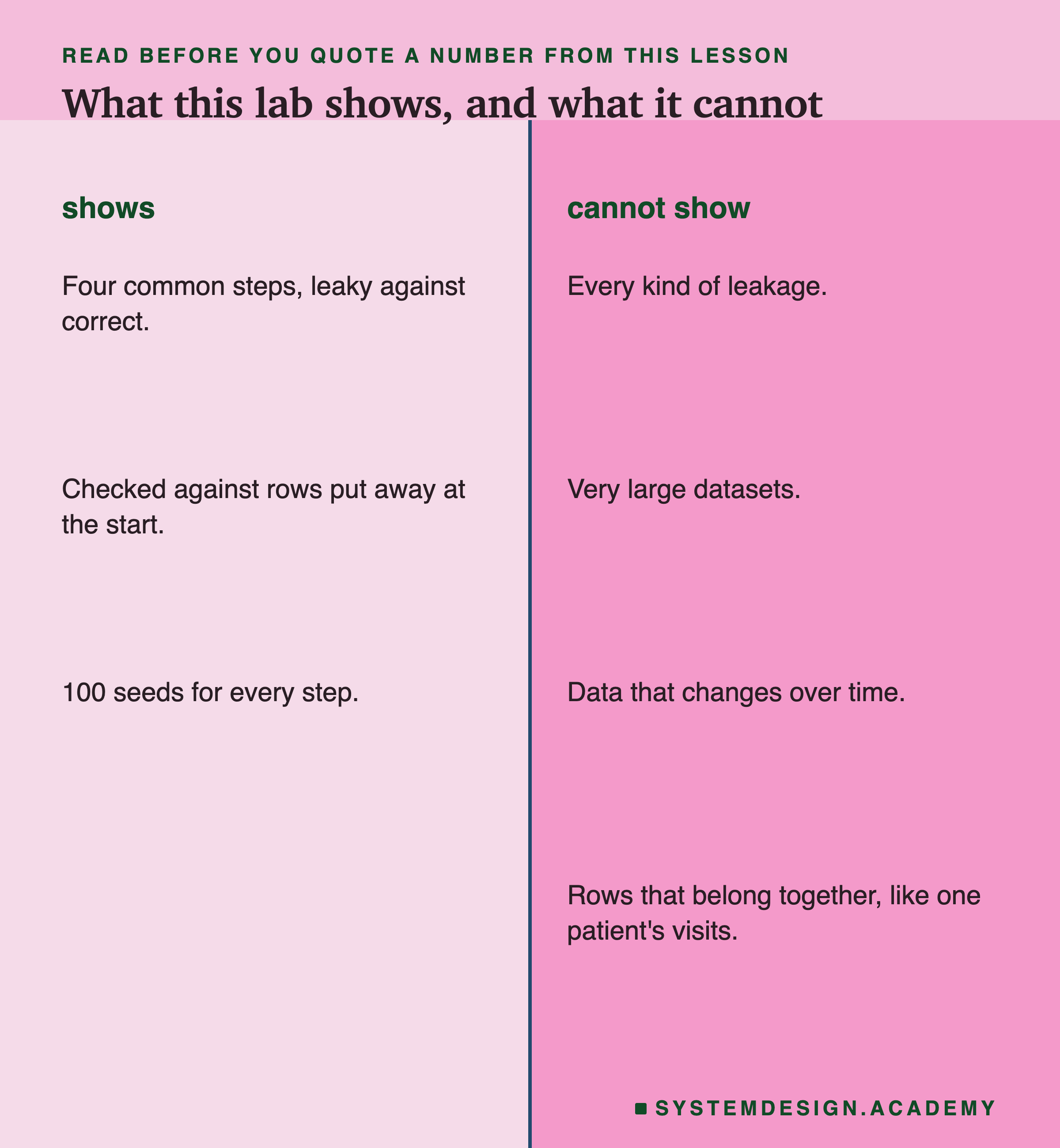
Four steps, not every kind of leakage. Filling gaps, removing unusual rows and choosing model settings are more steps that can leak. The lab did not test them.
Two of the four ran on pure noise. Noise makes a leak easy to see, because the honest answer is known. On real data the leak adds to a real pattern, and is harder to spot.
Rows that belong together. One patient's many visits, or one user's many sessions, can leak across a random split with no preparation step at all. The cure is to split by patient or by user. The lab did not test this.
Columns from the future. A column filled in after the outcome, like "account closed date" when predicting which customers leave, leaks with no preparation step at all. Moving steps inside the split will not help. For every column, ask whether it would exist at the moment the model has to predict.
Time. When data changes over time, the later rows should be the newest rows, not a random 30%.
Small data. The datasets here run from 100 to 569 rows. With many more rows some of these gaps may shrink; how much, this lab cannot say.
What to Do on Monday
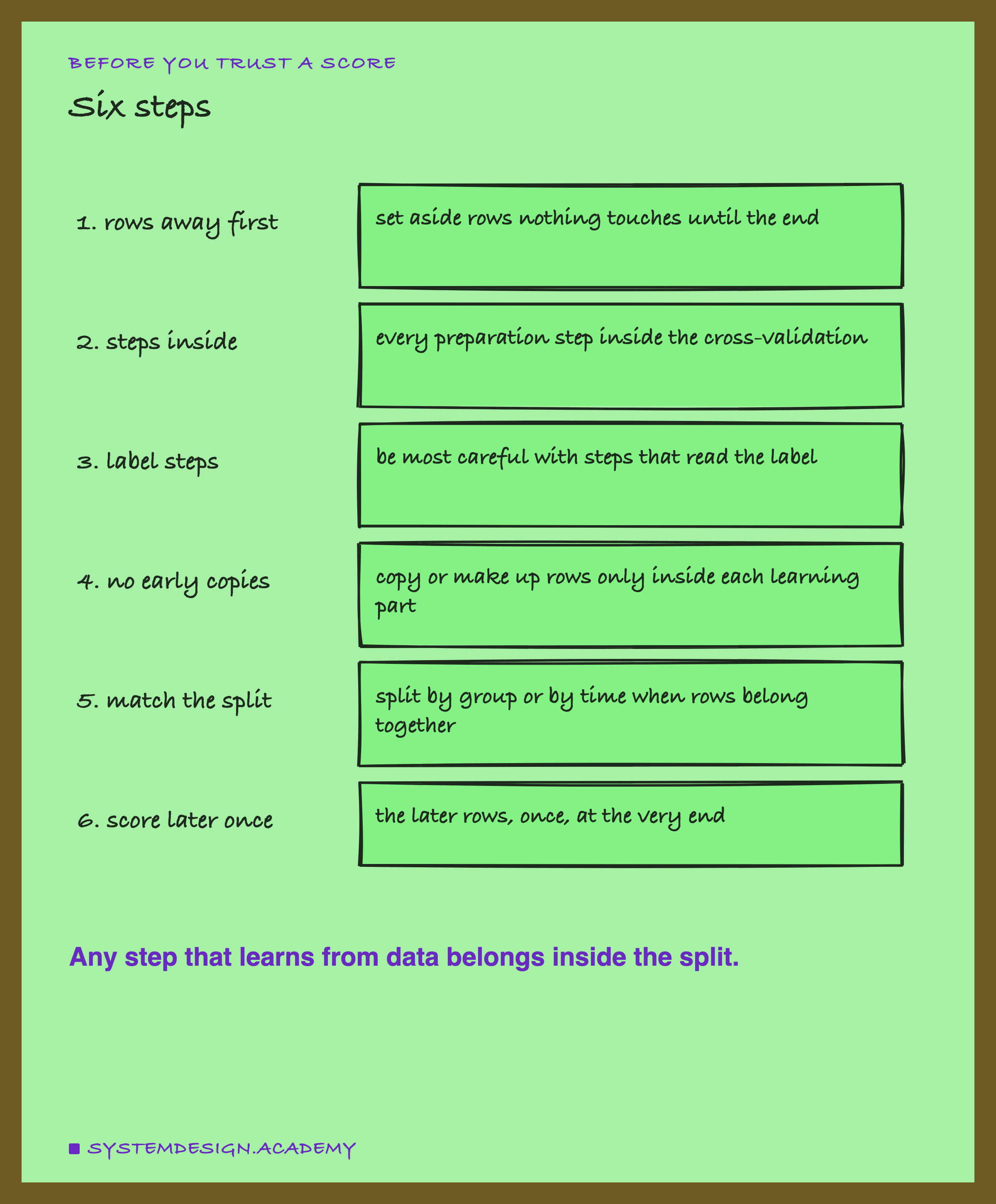
- Put later rows away first. Before any preparation, set aside rows that nothing will touch until the very end.
The names in brackets below are scikit-learn tools. You can look each one up when you need it.
-
Put every step inside the cross-validation. Build a Pipeline: one object that holds the preparation steps and the model together. Hand that whole Pipeline to the cross-validation tool (cross_val_score, or GridSearchCV when you are also trying settings), which trains it again on the learning rows of each fold. A Pipeline trained once on all the rows and then scored leaks just the same.
For copying rows, use the Pipeline from a second library, imbalanced-learn, because scikit-learn's own Pipeline cannot change the number of rows.
-
Be most careful with steps that read the label. Choosing columns by how well they match the label, and target encoding, leaked the most here. For target encoding, use TargetEncoder inside the Pipeline.
-
Never copy or make up rows before the split. Copying rows, and SMOTE, which makes up new rare rows between real ones, belong inside each learning part only.
-
Match the split to the data. If one patient or one customer has many rows, split by patient or customer (GroupKFold). If the data changes over time, test on the newest rows (TimeSeriesSplit, or a cut by date). If you choose model settings by cross-validation, the best score is itself a little too high, because the best of many tries is partly luck. Trust the later rows for the final number.
-
With a few dozen rows, that score can move by ten points on luck alone, so worry about a large gap, not a small one. If you change the recipe after looking, those rows are no longer untouched; keep a fresh set for the final check.
Knowledge Check
Knowledge Check
4 questions - Score 80% to pass
You choose the 20 best columns using all your rows, then cross-validate a model on them. The data is pure noise. What did this lab find?
Which of these preparation steps leaked the least in this lab?
Why do the steps that use the label leak the most?
How can you tell whether a cross-validation estimate is honest?