Picture an airport scanner. Almost every bag on the belt is ordinary. Once in a long while, one needs a closer look. The officer has two ways to catch more of the rare ones.
The first is to retrain the officer: show them hundreds of extra pictures of suspicious bags until those feel common. The second is simpler: turn the sensitivity dial on the machine, so it flags a bag at a lower level of suspicion.
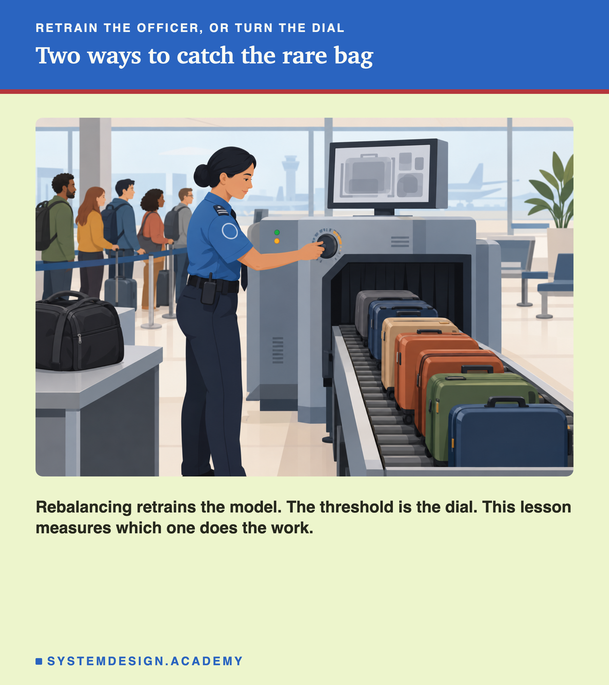
Machine learning has the same two choices when one class is rare, like fraud, disease or defects. You can rebalance the training data, or you can move the threshold, the dial. The imbalanced-data lesson describes both, and suggests starting with rebalancing and tuning the threshold last. In this lesson I measure them against each other, and the answer turns on something that lesson did not mention: how you set the dial.

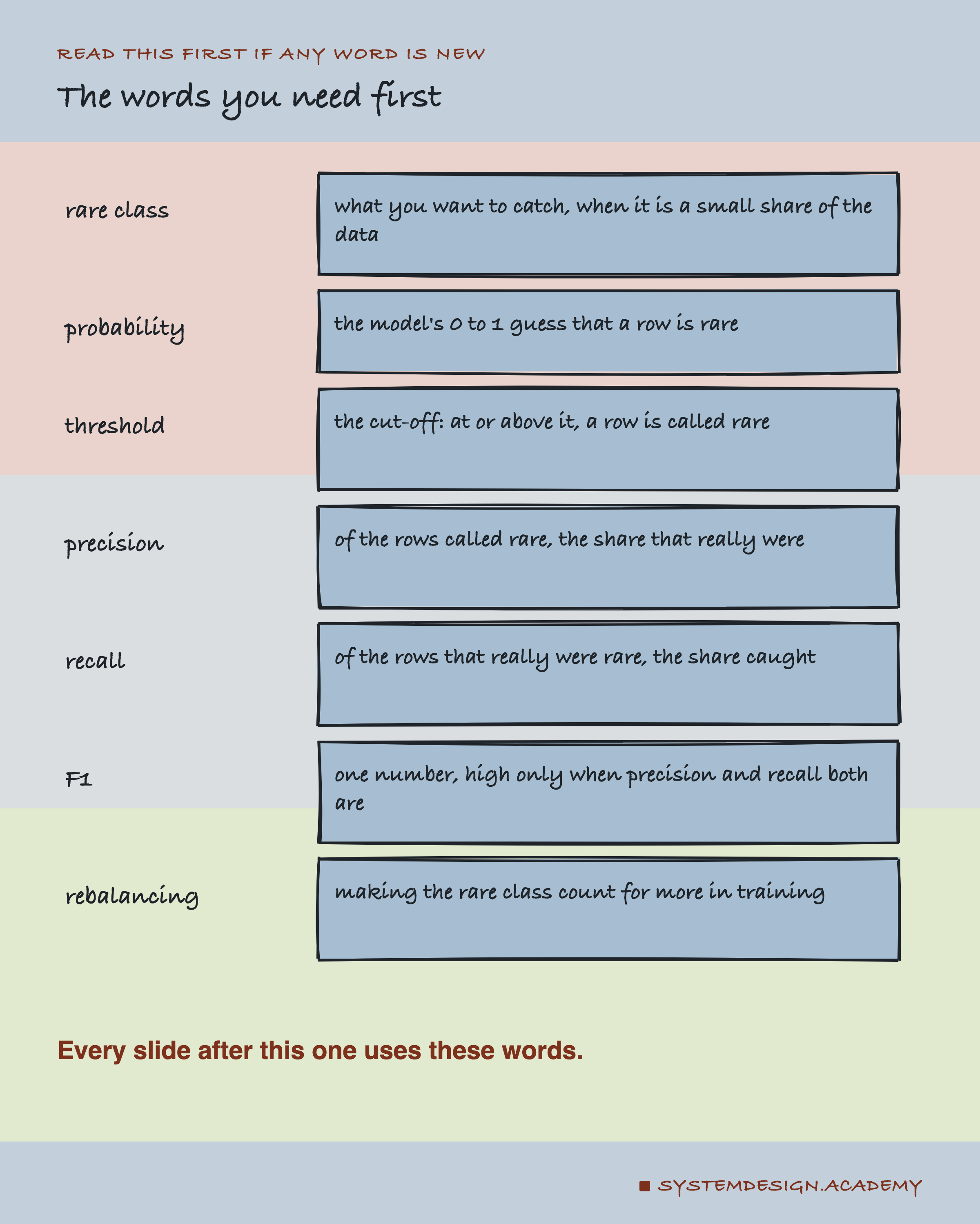
Rare class. The thing you want to catch, when it makes up only a small share of the data. Here, 2, 5 or 10 percent.
Probability. The model's output for each row: a number from 0 to 1 saying how likely it thinks the row is rare.
Threshold. The cut-off. Rows with a probability at or above it are called rare. The usual default is 0.5.
Precision. Of the rows the model called rare, the share that really were. Low precision means many false alarms.
Recall. Of the rows that really were rare, the share the model caught. Low recall means many misses.
F1. One number that combines precision and recall. It is high only when both are high.
Rebalancing. Changing the training data or the training rules so the rare class counts for more.
Training, validation and test sets. The model learns from the training set. The validation set is kept aside to make choices on, such as where to set the threshold. The test set is kept aside until the very end, to give a fair final score.
Seed. A starting number for the random shuffles, so a run can be repeated exactly. Each seed thins and splits the data differently.

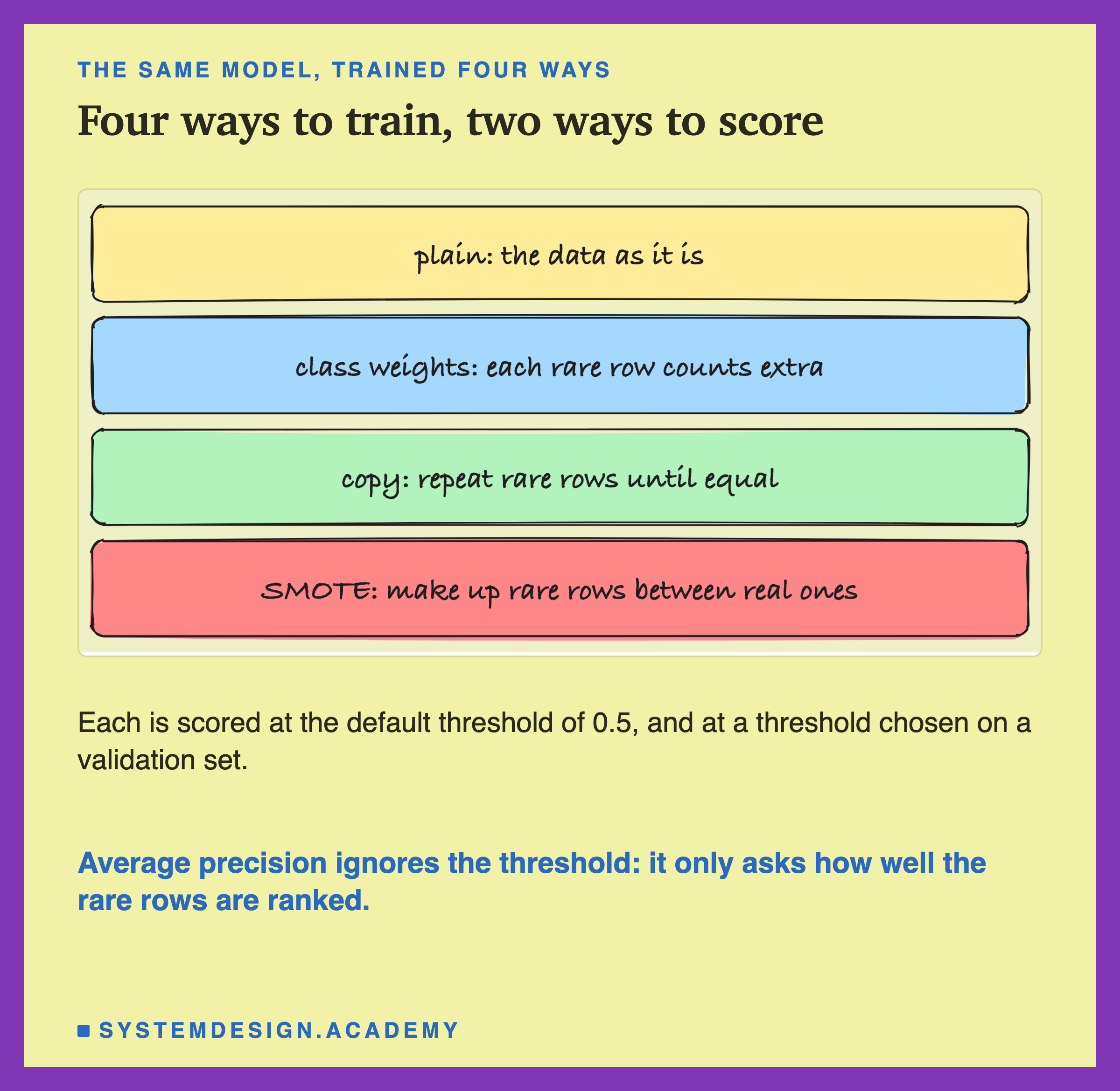
Every version uses the same kind of model, logistic regression: a simple model that draws one straight boundary between the classes and turns each row's distance from it into a probability.
Each version is scored on the test set in two ways: at 0.5, the default threshold, and tuned, at a threshold chosen without looking at the test set.
I also report average precision, or AP, the same idea as the PR-AUC from the imbalanced-data lesson. It ignores the threshold. It sorts every test row by its probability and asks how near the top the rare rows land. Two models with about the same AP can usually reach similar results, each with its own threshold.
Here is the procedure behind every "tuned" number in this lesson.
The last step is the one people skip. If you chose the threshold by looking at the test set, you would be marking your own exam.
There is a catch. If the validation set holds only one or two rare rows, many thresholds give the same F1, and the "best" one is close to a guess.
The fifth version answers that with cross-validation. It splits the training data into 5 parts. For each possible threshold, it trains a model on 4 parts, measures F1 on the fifth, repeats that for all 5 parts, and averages. It keeps the threshold with the best average, then trains one final model on all the training data and uses that threshold with it. So the threshold is judged on every rare training row, not just the one or two in validation. scikit-learn does this with a tool called TunedThresholdClassifierCV.

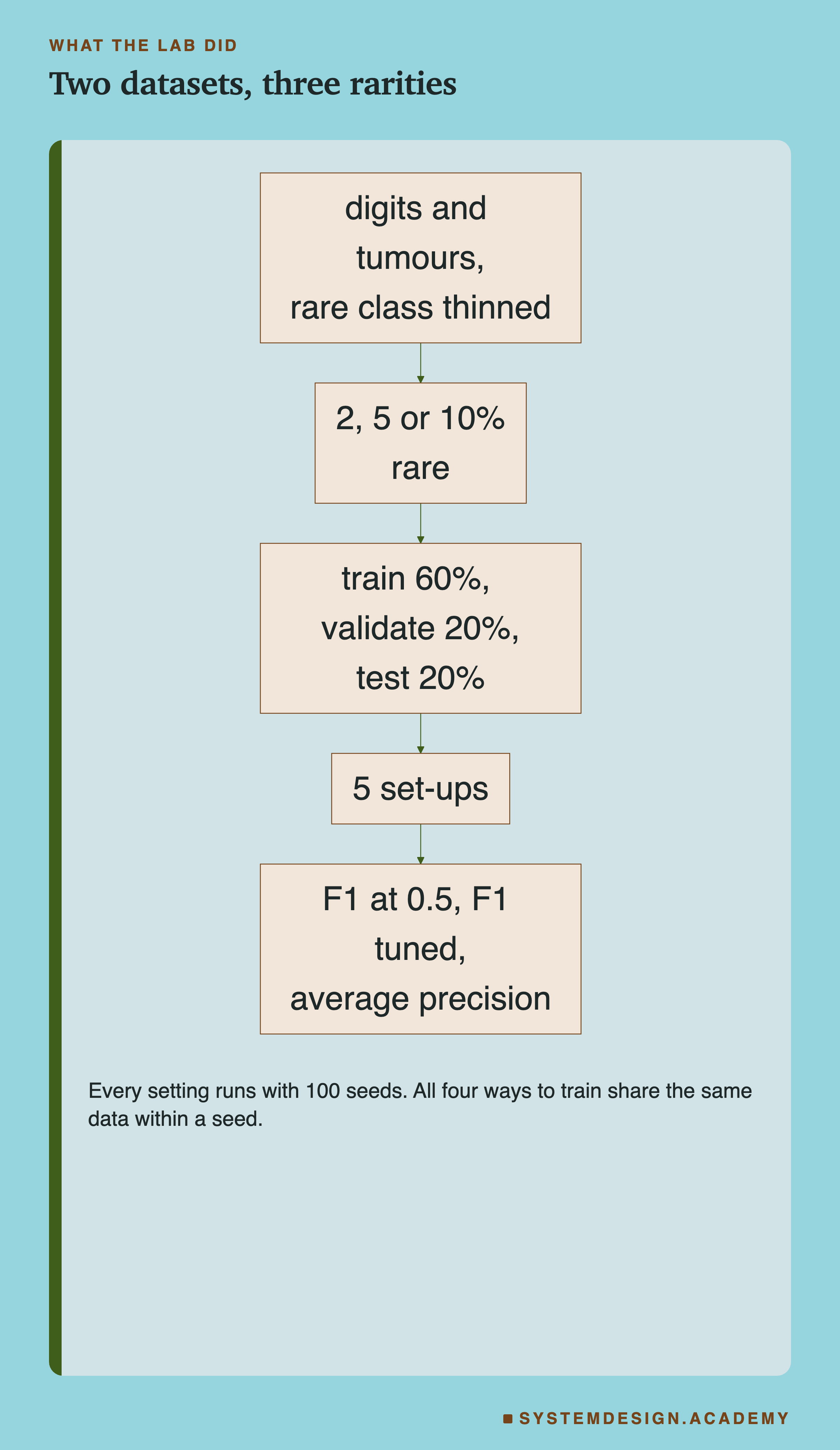
The data. Two real datasets that come with scikit-learn, a free Python library. Handwritten digits, where the rare class is the digit 9. And breast tumour measurements, where the rare class is malignant.
The rarity. I thinned out the rare class until it was 2, 5 or 10 percent of the data. This happens before splitting, so the test set is just as rare as the training set.
The split. 60 percent training, 20 percent validation, 20 percent test.
The runs. Every setting ran with 100 different seeds. All five versions share the same data within a seed, so they can be compared seed by seed.
A warning about size. The tumour dataset is small. At 2 percent rare, a test set held only about 2 rare rows, and the validation set about the same. The digits held about 7 at 2 percent. That difference turns out to matter more than anything else in this lesson.
One correction. My first run broke ties between thresholds by taking the lowest one. A reviewer showed that this pushed the tuned threshold down whenever there were few rare rows, and made tuning look worse on the tumours. Every number here comes from the corrected run.
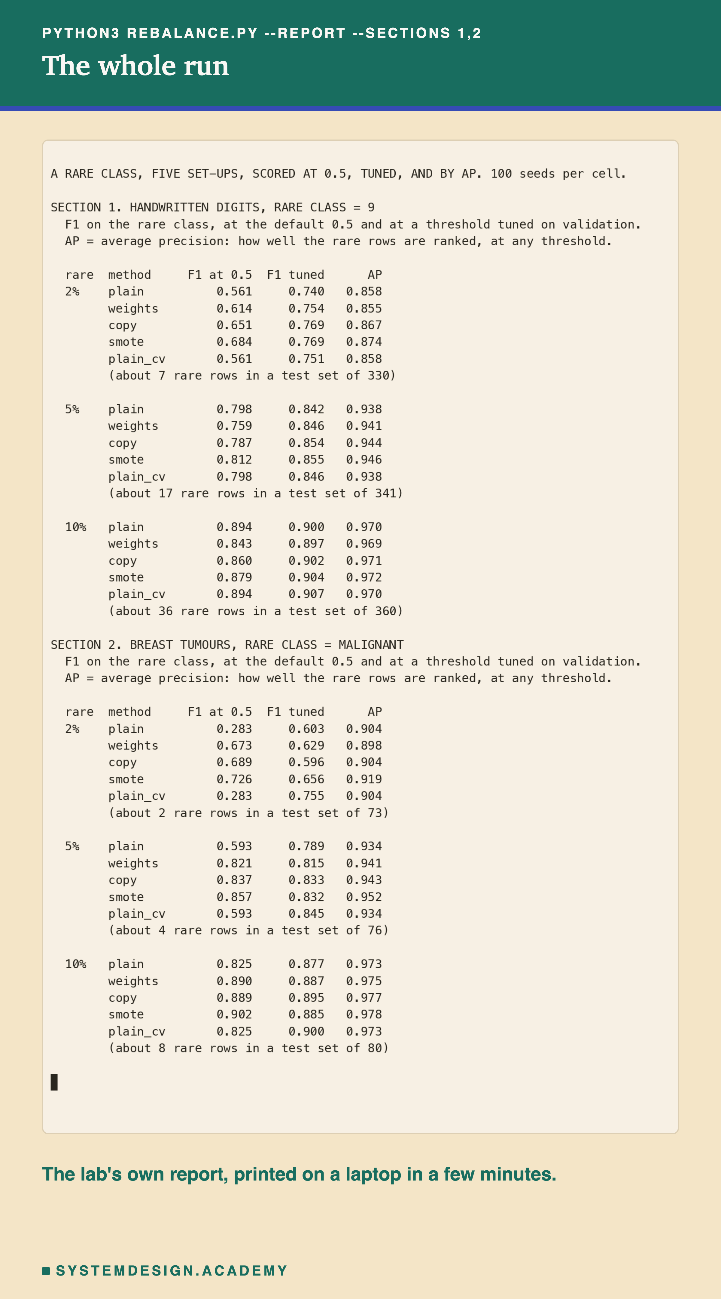
This is a real recording of the lab's report, printed on the laptop where it ran. The whole lab takes a few minutes on a laptop.

In the recording, "weights" is class weights, "copy" is copying rare rows, and "plain_cv" is the plain model with a cross-validated threshold. For plain_cv, "F1 at 0.5" is simply the plain model, since only its threshold differs.

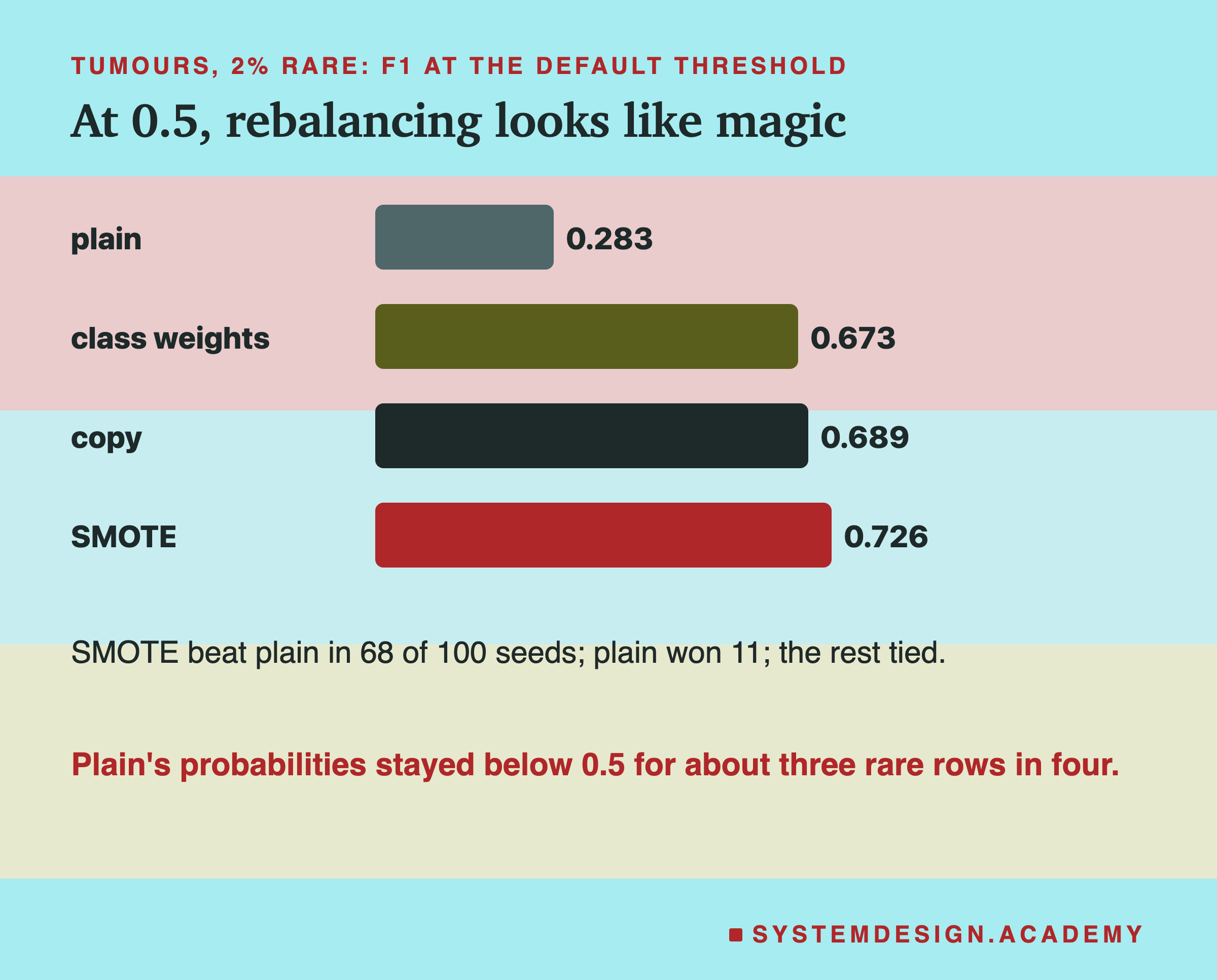
| tumours, 2% rare | plain | class weights | copy | SMOTE |
|---|---|---|---|---|
| F1 at 0.5 | 0.283 | 0.673 | 0.689 | 0.726 |
Start at the default threshold, because that is where most people stop. With 2 percent malignant tumours, the plain model scored an F1 of 0.283. Every way of rebalancing more than doubled it. SMOTE beat plain in 68 of 100 seeds, plain won 11, and the rest were ties.
Here is how to read that "by luck" idea, which comes up again below. Treat each seed as a coin flip for which method scores higher, leaving out the ties. If the two methods were truly equal, a split this uneven would happen by chance less than once in a million tries.
Why is plain so poor here? A model trained on data that is 98 percent common learns that "common" is almost always right. Its probabilities for the rare rows stay low, so at 0.5 its recall was only 0.255, about one rare tumour in four, against 0.825 for SMOTE. Rebalancing pushes those probabilities up. Moving the threshold down has the same effect on which rows get called rare, without changing any probability.

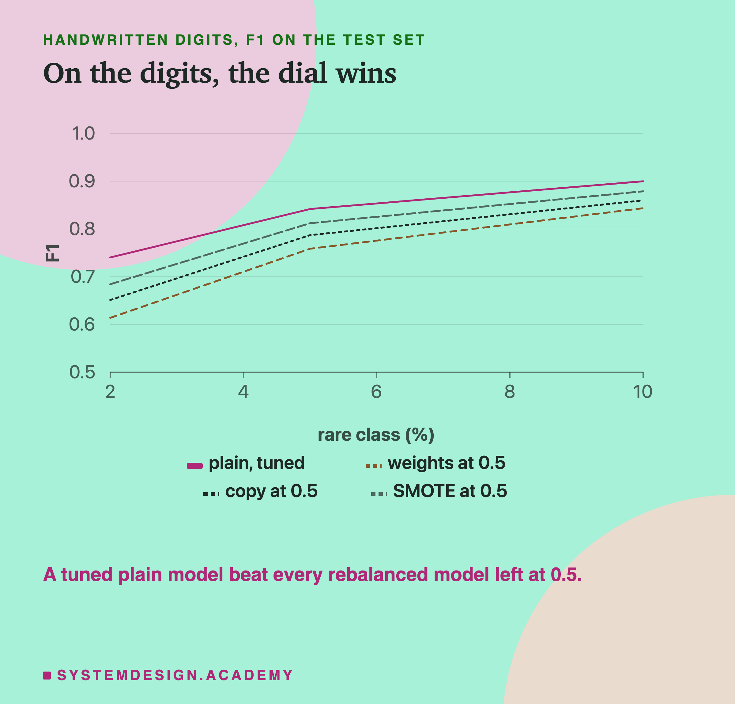
| digits | plain, tuned | weights at 0.5 | copy at 0.5 | SMOTE at 0.5 |
|---|---|---|---|---|
| 2% rare | 0.740 | 0.614 | 0.651 | 0.684 |
| 5% rare | 0.842 | 0.759 | 0.787 | 0.812 |
| 10% rare | 0.900 | 0.843 | 0.860 | 0.879 |
On the digits, a plain model with its threshold tuned on validation beat every rebalanced model left at 0.5, at every rarity. Against class weights at 2 percent, the tuned plain model was higher in 86 seeds and lower in 11. Against SMOTE at 0.5, also at 2 percent, it was higher in 68 and lower in 26.
Once each method had its own tuned threshold, the four landed close together: 0.842 for plain and between 0.846 and 0.855 for the others at 5 percent. Most of what rebalancing seemed to do at 0.5, the dial did on its own.

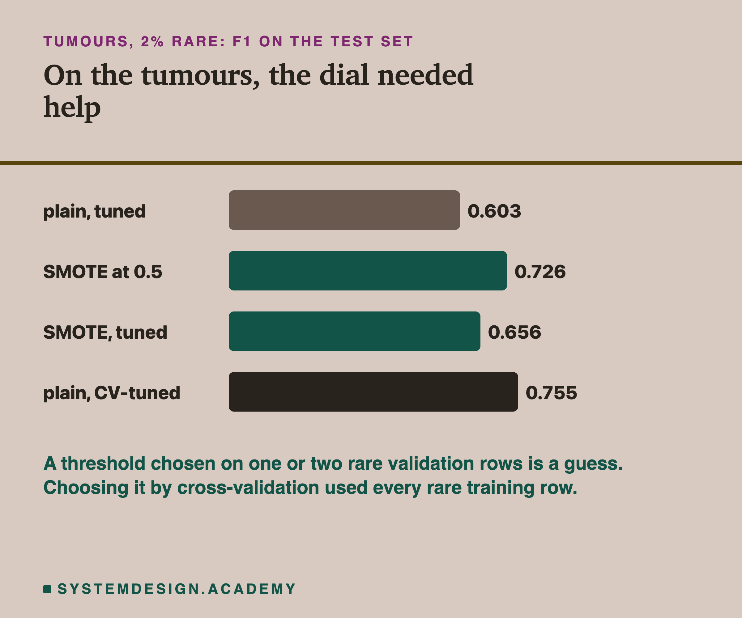
| tumours, 2% rare | F1 |
|---|---|
| plain, tuned on validation | 0.603 |
| SMOTE at 0.5 | 0.726 |
| SMOTE, tuned on validation | 0.656 |
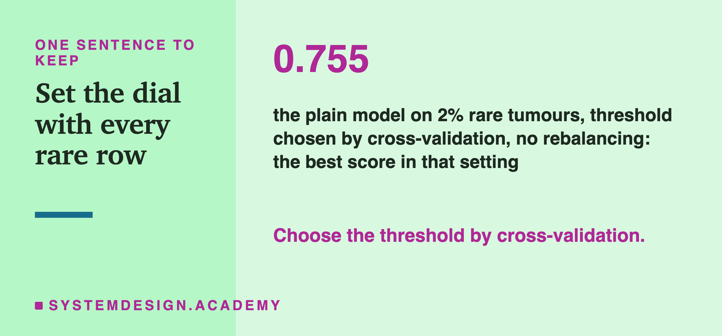
| plain, cross-validated threshold | 0.755 |
The tumours tell a different story. Tuning on validation lifted the plain model to only 0.603, below SMOTE left at 0.5, and tuning even made SMOTE worse, 0.726 down to 0.656. With one or two rare rows in the validation set, the chosen threshold was close to a guess.
The fix was not to rebalance. It was to choose the threshold on more rare rows. The plain model with a cross-validated threshold scored 0.755, the best of all. Against the plain model tuned on validation, it was higher in 44 seeds and lower in 11, which chance gives about once in 114,951 tries. Against SMOTE at 0.5 it was higher in 26 and lower in 20, about even.
On the digits, the cross-validated threshold did about as well as tuning on validation: higher in 37 seeds and lower in 32 at 2 percent, and just as even at 5 and 10 percent. So it never did worse here, and on the small tumour data it did much better.

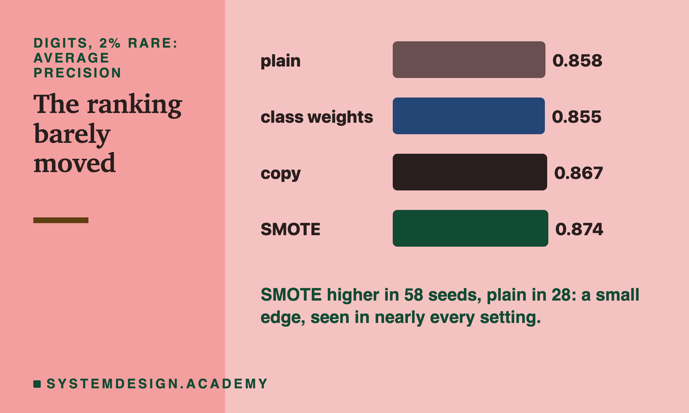
If rebalancing mostly shifts probabilities up, the ranking should hardly change, and average precision measures exactly the ranking. On the digits at 2 percent, AP was 0.858 for plain, 0.855 for class weights, 0.867 for copy and 0.874 for SMOTE.
SMOTE did nudge AP up a little almost everywhere, by up to about 0.02. On the digits at 2 percent it was higher in 58 seeds and lower in 28.
The lab made 96 seed-by-seed comparisons in all, every method against plain on every dataset, rarity and score, so one result that strong could be luck on its own. What makes it believable is that SMOTE's AP came out ahead in nearly every setting. Two reasons are possible: the made-up rows give the model a fuller picture of the rare class, or doubling the training rows weakens the model's regularisation, a built-in penalty that stops it leaning too hard on any single pixel or measurement. This lab cannot separate them.
On the tumours, treat AP as weak evidence. With one or two rare rows in a test set, the plain model scored a perfect AP of 1.0, every rare row ranked above every common one, in 75 of 100 runs at 2 percent, so AP had little room to move either way.
One cost of rebalancing is easy to miss. After it, a probability of 0.8 no longer means 8 in 10 such rows are rare, because the model was trained on a world where rare rows were common. If anything downstream reads the number as a real probability, like a risk score shown to a doctor, you must correct it again, a step called calibration. Moving the threshold leaves the probabilities honest.
At the default threshold, rebalancing was not always a help. On the digits at 10 percent rare, every method lost to plain at 0.5: 0.894 for plain, against 0.843 for class weights, 0.860 for copy and 0.879 for SMOTE.
Look at class weights at 5 percent to see why. Recall rose from 0.682 to 0.954, so it caught more 9s. But precision fell from 0.979 to 0.635, so it raised many more false alarms. When the rare class is not that rare, making it count as much as everything else overshoots. A tuned threshold pulled it back: class weights with a tuned threshold scored 0.846, against 0.842 for plain with a tuned threshold.
This box holds the lab's real per-run results for 2 and 5 percent rare: for each dataset and way to train, 100 runs of F1 at the default threshold, F1 at the tuned threshold, and average precision. Press Run to compare one version with plain, seed by seed.
Then change the settings. Try METHOD = "plain_cv" with SCORE = "f1_tuned", then DATA = "digits".
The last line is a chance written as a decimal: 3.5e-11 means far less than once in a billion, and 0.8 means 8 times in 10, which is easily luck. A tie means both scored exactly the same, which happens often when a test set holds only one or two rare rows.

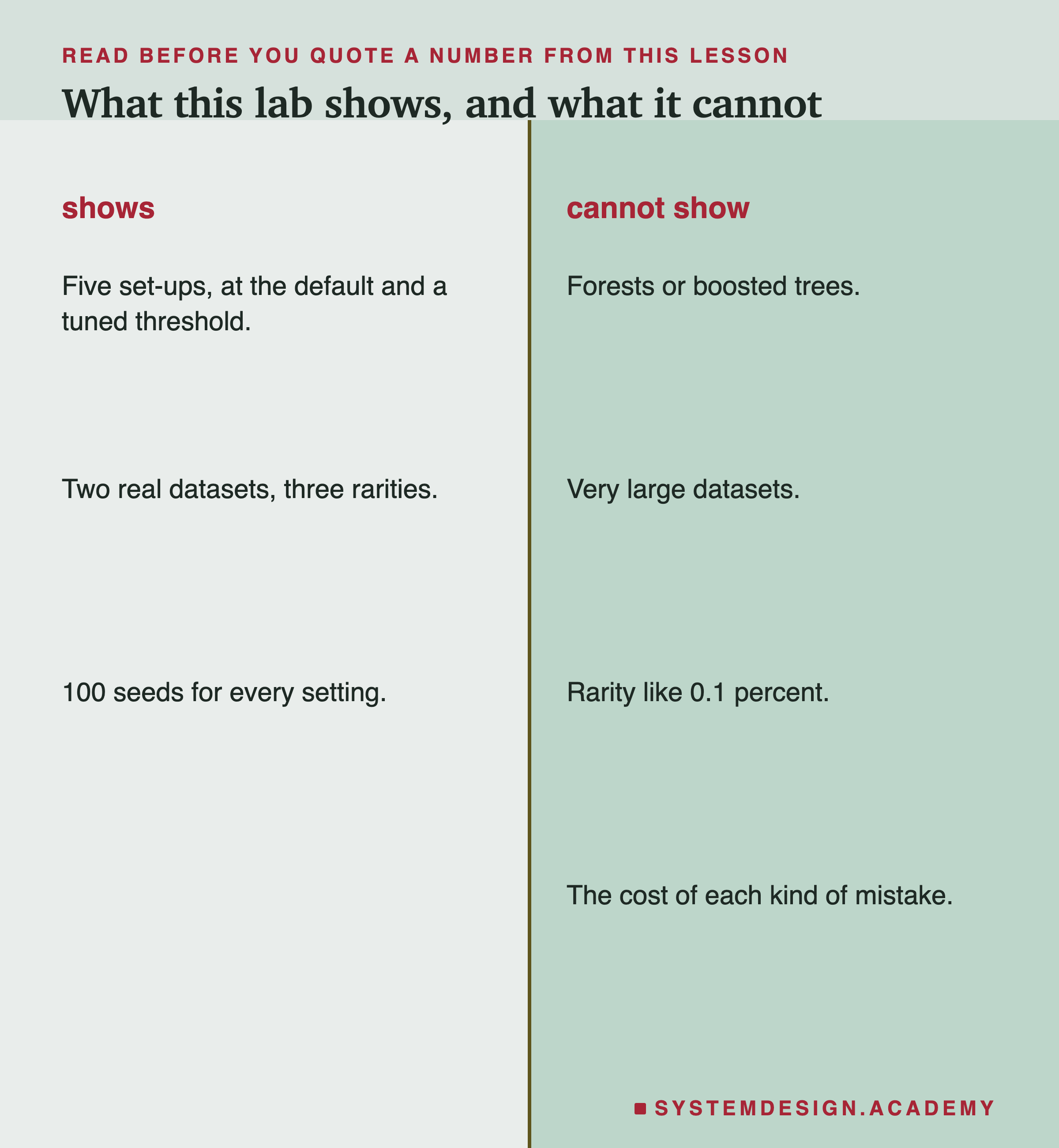
One kind of model. For logistic regression, rebalancing mostly slides every probability up by about the same amount, so it is the model most likely to show "the threshold does the same job". Random forests and boosted trees choose their splits using counts of rows, so rebalancing can change what they learn. Test the claim on your own model.
One setting for regularisation. The model's built-in penalty was not retuned for each version, and copying or SMOTE nearly doubles the training rows, which weakens that penalty.
Few rare rows, not just a low percentage. Thinning threw rare rows away, so the tumour models trained on about 4 of them at 2 percent. The count of rare rows drives these results as much as the percentage. A problem that is 0.1 percent fraud but has 5,000 fraud cases is better placed than this lab.
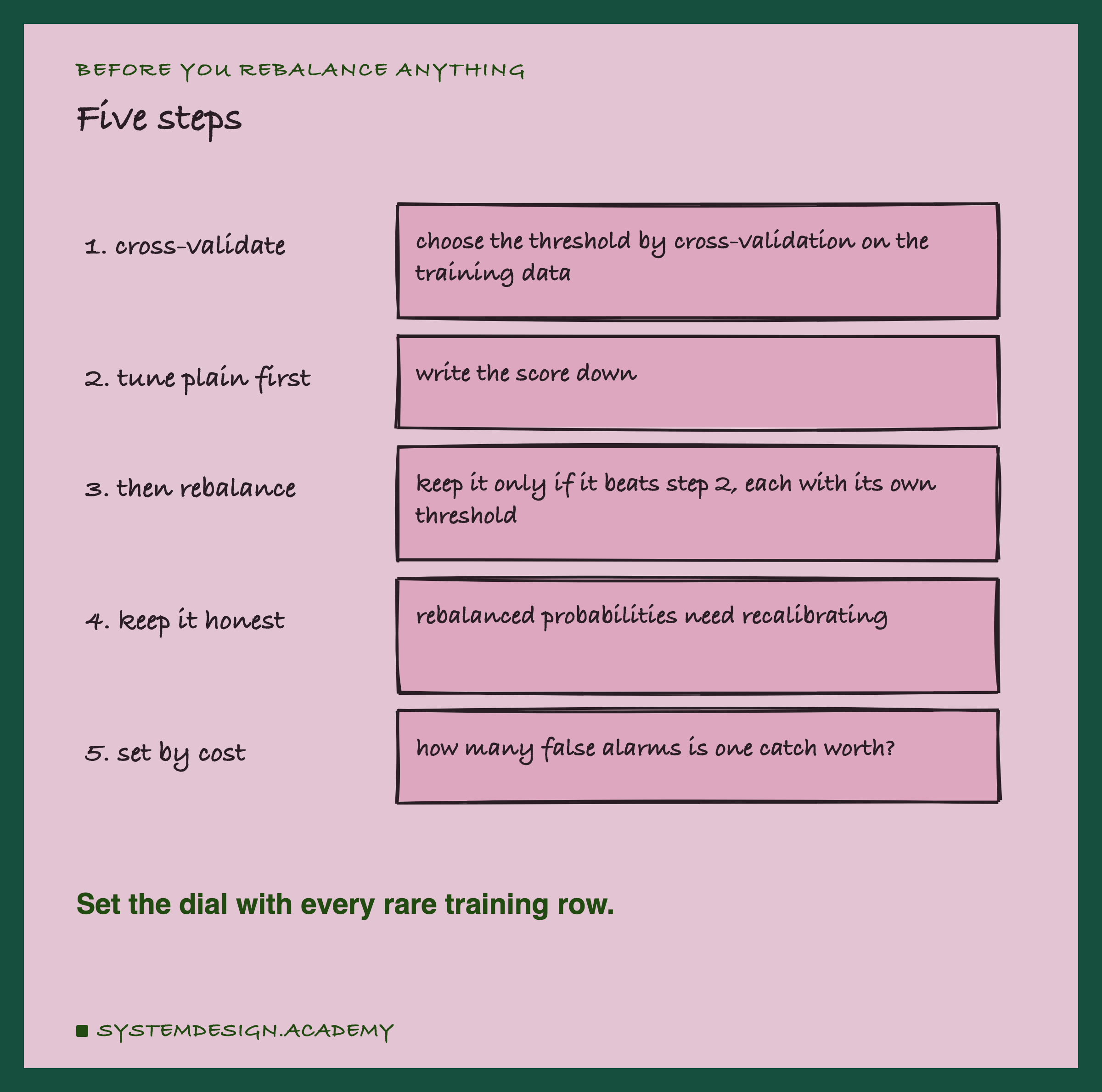
F1 treats both mistakes as equal. A missed tumour usually costs far more than a false alarm. Every threshold here was chosen for the best F1. In a real system you would choose it by cost instead, as the last step on the next slide shows.
Many comparisons. The lab made 96 seed-by-seed comparisons. A single result near "once in 100 tries" can be luck among that many.

Choose the threshold by cross-validation on the training data, for example with scikit-learn's TunedThresholdClassifierCV. Here it matched tuning on a validation set when that worked, and beat it clearly when the validation set held only a handful of rare rows.
Do that on the plain model first, and write the score down. On the digits, a tuned plain model beat every rebalanced model left at 0.5.
Then try rebalancing, each with its own well-chosen threshold, and keep it only if it beats step 2. Never judge rebalancing at the default 0.5.
Keep the probabilities honest. If anything reads the model's number as a real probability, prefer moving the threshold, or recalibrate after rebalancing.
Set the final threshold by cost, not F1. Decide what a false alarm and a miss each cost you. With honest probabilities, flag a row when its probability is above: cost of a false alarm divided by (cost of a false alarm plus cost of a miss). If a miss costs 99 times as much as a false alarm, that threshold is 0.01.

The dial did most of the work. It stumbled only when I set it using a handful of rare validation rows, and cross-validation fixed that without touching the training data.
4 questions - Score 80% to pass
At the default threshold of 0.5, a plain model on 2 percent rare tumours caught only about one rare case in four. Why?
On the tumours, a threshold tuned on the validation set did badly. What fixed it?
Why can rebalancing be a problem if a doctor reads the model's number as a risk?
Class weights raised recall but lowered F1 at 0.5 on digits at 5 percent rare. What happened?