Picture a weather forecaster in a desert town. Every morning he says the same thing: no rain today. It rains on maybe two days a year. So he is right on about 363 days out of 365, more than 99 percent of the time. He has never once warned anyone to bring an umbrella.

Is he a good forecaster? By the count of right answers, he is excellent. By the one thing people need from him, he is useless. The rare day is the whole reason to have a forecaster.

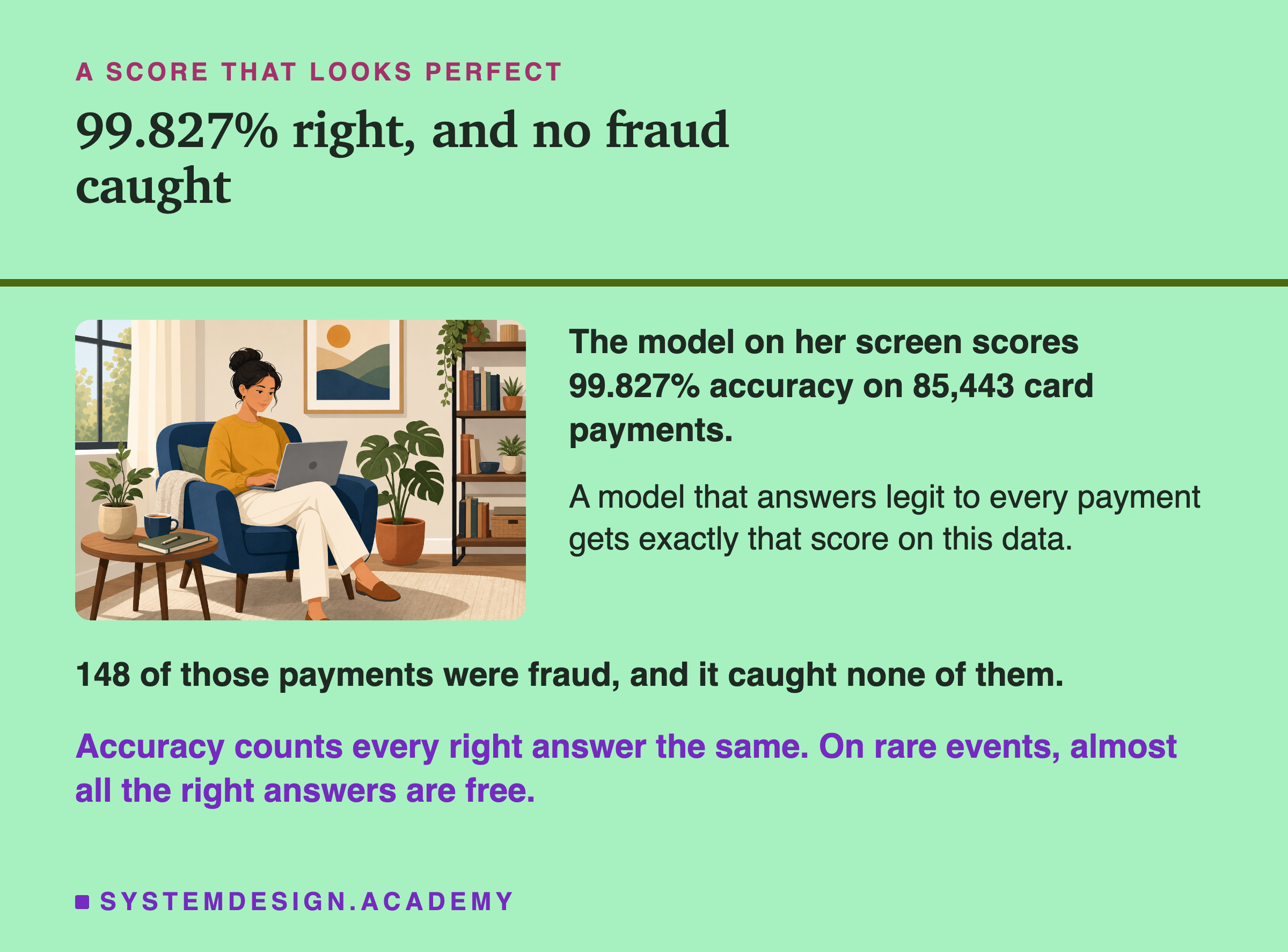
Machine learning has the same trap. When one kind of case is rare, a model can score very well by never naming it. In this lesson I measure that on real card payments. A model that calls every payment legit scores 99.827 percent on the test set and catches none of the 148 frauds.

In real work the rare case is often the one that matters: fraud, a rare disease, a broken part on a factory line. This lesson is about how to tell when a score is lying to you, which number to read instead, and what the common fixes really do. It ends with the other half of the title: messy data, such as copied rows and gaps, which can quietly bend every score you read.

This is the eighth lesson of the chapter on data engineering for machine learning. Lesson 7, on data labeling, was about where labels come from. This lesson is about what happens when one label is far rarer than the other.

Two later lessons in this chapter measure parts of this story in depth, and I build on them here rather than repeat them. Lesson 12, rebalance or threshold, compared rebalancing the data with simply moving the model's cut-off. On average, a plain model with a well-chosen cut-off beat rebalanced models left at the default. Lesson 13, leakage before the split, measured how much each preparation step leaks when it runs before the data is split.

What this rebuild corrected. An earlier version of this lesson made claims its sources do not support. Each is fixed where it comes up, and the full record is in results/ibl-factcheck.json.

• It opened with a fraud team's story. It was made up, and so were the confusion matrices and curves that followed it.
• It said fraud is "roughly 1 transaction in 1000" in a typical payments stream. I found no source. The real public data used here is 0.173 percent.
• It said ROC-AUC is "flatteringly high" on rare classes. More exactly, it does not move when only the rarity changes. That is a different problem, measured below.
• It said fitting an imputer on all rows turned a 0.95 score into 0.62 in production. Those numbers were invented, and lesson 13 measured that rescaling, a similar step, barely leaked.
• It said to start with class weights or SMOTE and tune the threshold last. Lesson 12 measured the opposite order working better.

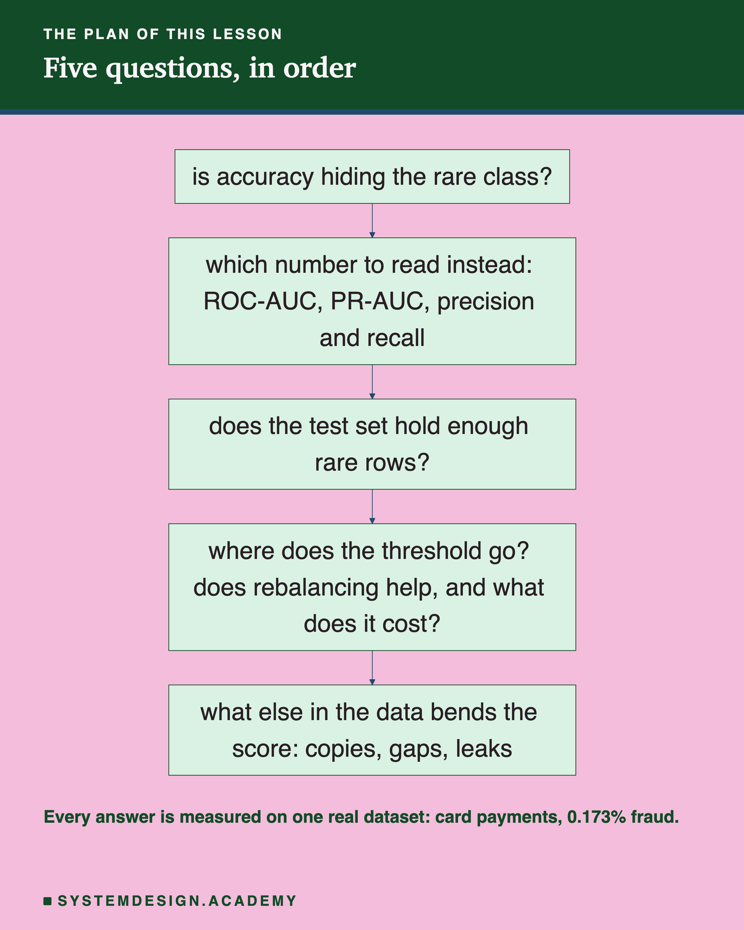
The plan follows that chart from top to bottom. First the trap itself, then the two numbers people use in place of accuracy and how they behave as the rare class gets rarer. Then the split, the cut-off and rebalancing, each with a real measurement. Last, the messy data: copies, gaps and leaks.

Accuracy is the share of all answers that were right. The rare class is the thing you want to catch, when it makes up a small share of the data. Here it is fraud.

Precision is, of the rows the model flagged as fraud, the share that really were fraud. Low precision means many false alarms. Recall is, of the rows that really were fraud, the share the model flagged. Low recall means many misses.

Most models do not answer yes or no. They give a probability, a number from 0 to 1. The threshold is the cut-off: a row above it is flagged. scikit-learn uses strictly above; this lesson's lab counts at or above, which differs only for a row exactly on the line. In scikit-learn, a popular Python library for machine learning, the default threshold is 0.5.

ROC-AUC and PR-AUC grade the ranking itself, across every threshold. I explain both properly on their own slide. A stratified split is a split that keeps the same share of rare rows on each side. Class weights make each rare row count more while the model learns. A probability is calibrated when it means what it says: rows given 0.2 turn out rare about 2 times in 10.

I wrote the lab's design into the docstring of its script, imbalance_demo.py, on 1 October 2026, before it ran. The script is the one you can copy from this lesson. Before writing the design, I loaded the data once to see its columns and count exact copies. I also fitted two models on one split to check the plan could run. Nothing else ran first.

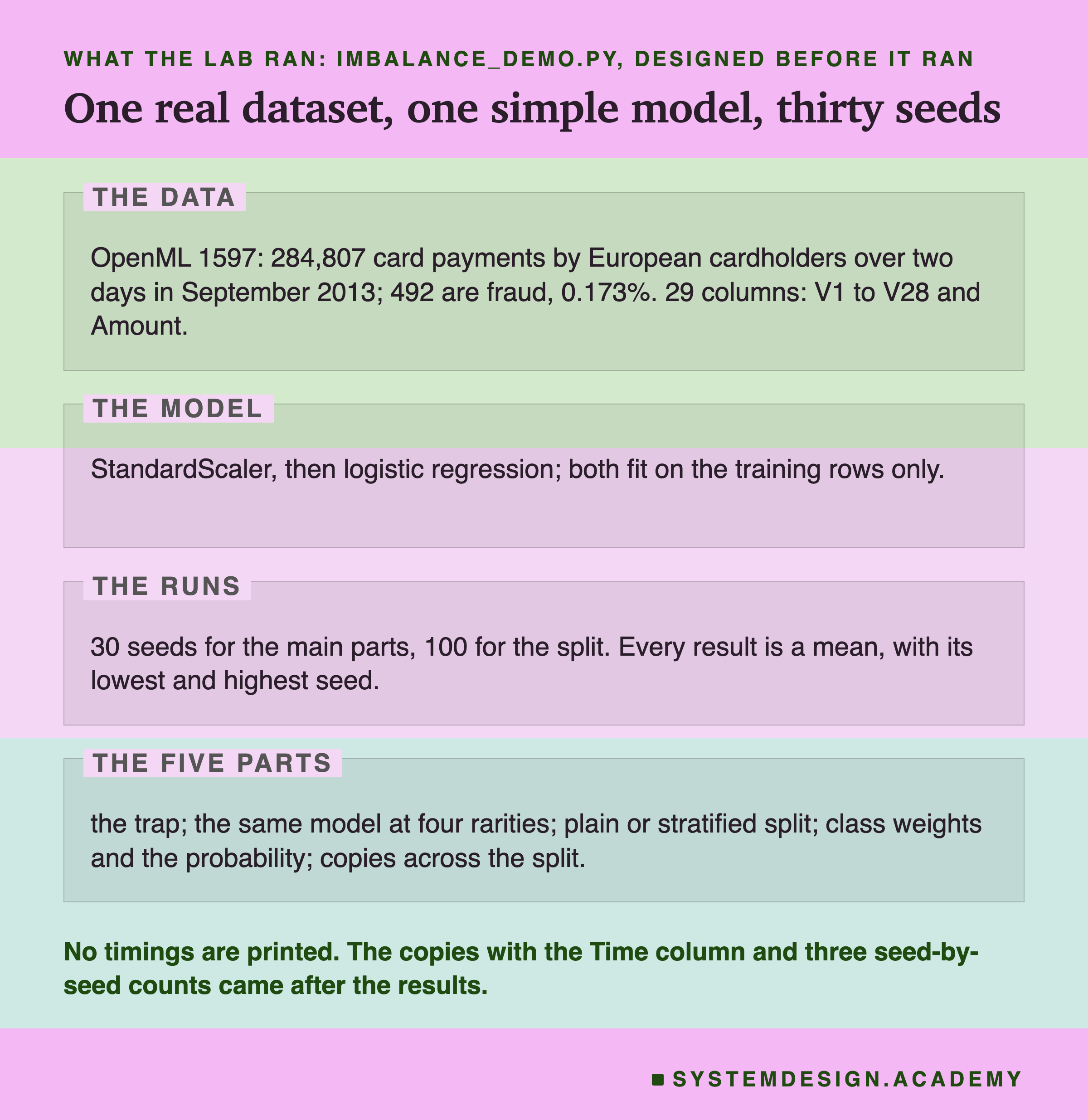
The data is a public set of card payments, published by a research group at the Université Libre de Bruxelles with the payments company Worldline. In its own words: "transactions made by credit cards in September 2013 by european cardholders", over two days, with "492 frauds out of 284,807 transactions". That is 0.173 percent fraud.

The columns are not readable. To protect the cardholders, the publishers turned the original fields into 28 new columns, V1 to V28. They used a method called PCA, which mixes the original columns into new ones. Only the time and the amount were left as they were. OpenML, the site the script downloads from, marks the time column as a row label, so scikit-learn leaves it out.

The model is logistic regression, which is a simple model that draws one straight boundary between the classes and turns each row's distance from it into a probability. Before it, a step called StandardScaler puts every column on the same scale. Both are fitted on the training rows only.

The runs. Each part runs with 30 different seeds. A seed is a starting number for the random choices, so each seed splits the data differently. One split is one draw, and one draw is not a finding, so every number below is a mean with its lowest and highest seed.

Here is the trap, measured. With seed 0, the test set held 85,443 payments, and 148 of them were fraud.

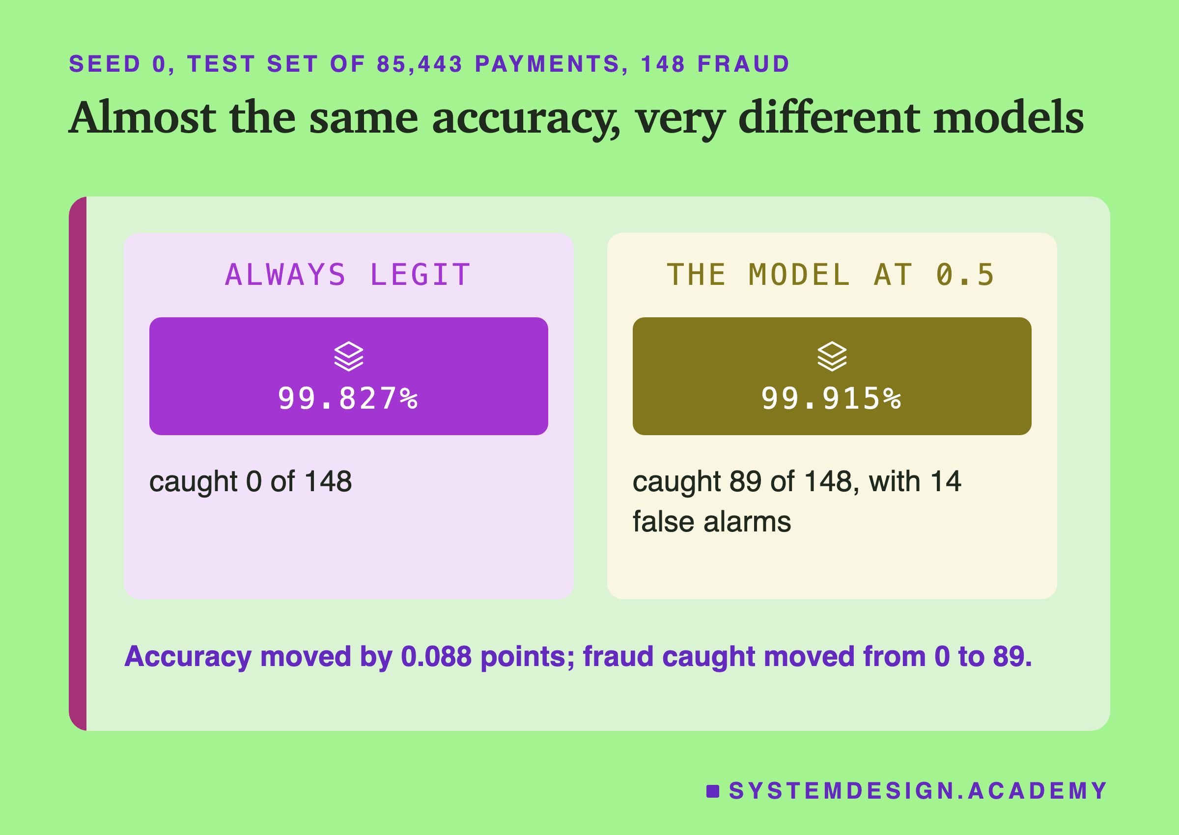
A "model" that answers legit to every payment scored 99.827 percent accuracy and caught nothing. The trained model, at the default threshold of 0.5, scored 99.915 percent. It caught 89 of the 148 frauds and raised 14 false alarms. Over all 30 seeds, the trained model averaged 99.918 percent and always-legit 99.827 percent.

So accuracy moved by less than a tenth of a point, while the number of frauds caught went from 0 to 89. If you only had the accuracy, you could barely tell a working model from one that does nothing. The dataset's own page on Kaggle, a site for sharing data, warns about exactly this: "Confusion matrix accuracy is not meaningful for unbalanced classification."

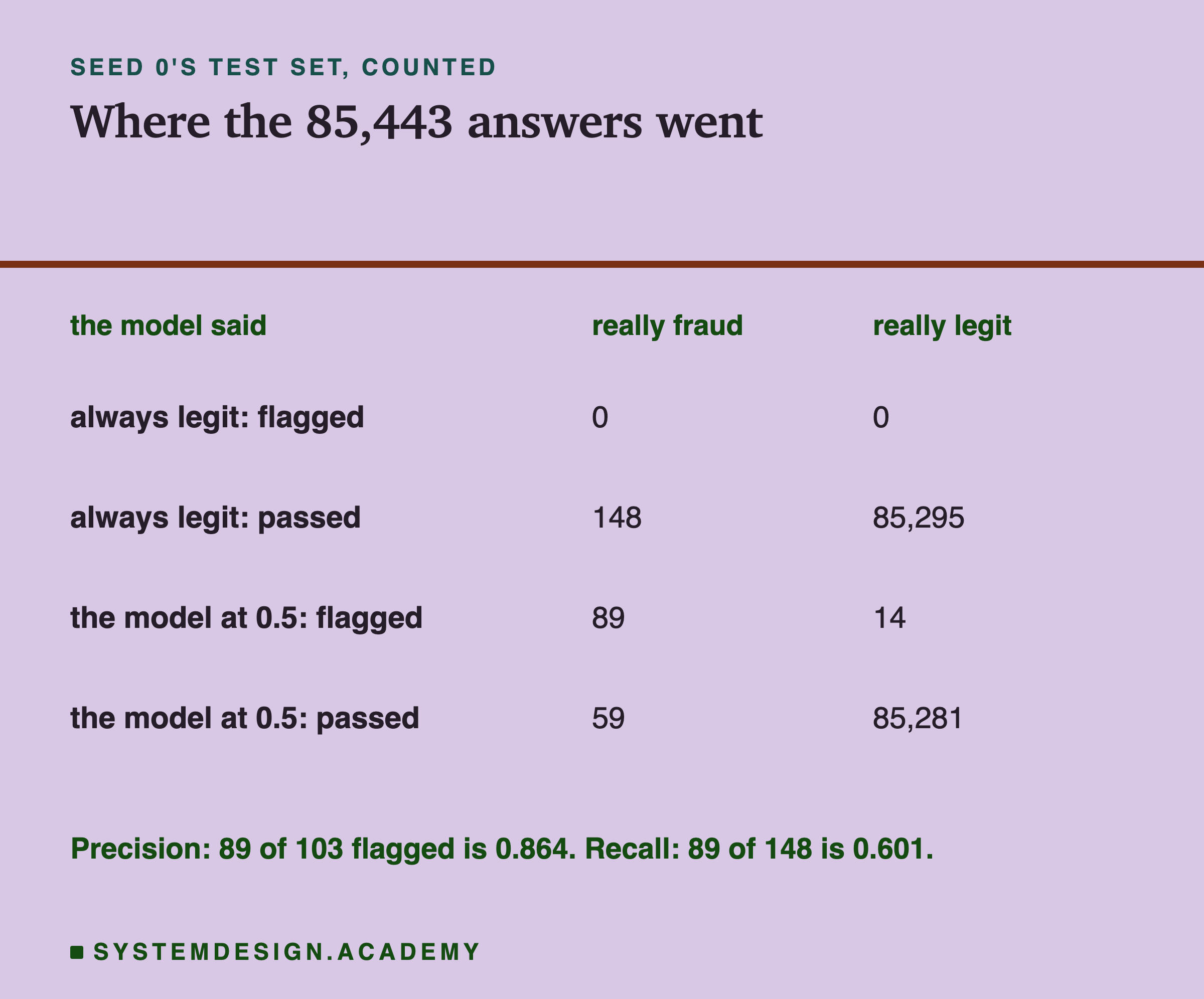
The table splits every answer by what the model said and what was true. This kind of table is called a confusion matrix. Accuracy only adds up the two "right" cells: flagged fraud and passed legit. Precision and recall look only at the fraud side of it, which is where all the useful information is.

Formulas are easier to trust once you fill them in yourself. Every number here comes from the table above.

Always legit. It flags nothing. So it gets every legit payment right, 85,295 of them, and every fraud wrong. Accuracy is 85,295 ÷ 85,443 = 0.99827, or 99.827 percent. Recall is 0 ÷ 148 = 0. Precision has no answer, because it flagged nothing: 0 ÷ 0.

The model at 0.5. It flagged 89 + 14 = 103 payments. Right answers are the 89 frauds it caught plus the legit payments it passed: 85,295 − 14 = 85,281. So accuracy is (89 + 85,281) ÷ 85,443 = 85,370 ÷ 85,443 = 0.99915, or 99.915 percent.

Now compare the two by right answers. The model got 85,370 right, and always-legit got 85,295. The difference is 75 answers, and 75 is exactly 89 − 14: it gained 89 by catching frauds and lost 14 by raising false alarms. Out of 85,443, 75 answers is less than a tenth of a percent.

Precision is 89 ÷ 103 = 0.864: about 86 of every 100 flags were real fraud. Recall is 89 ÷ 148 = 0.601: it caught about 60 of every 100 frauds. Those two numbers say what the model does. The accuracy mostly says how rare fraud is.

Precision and recall depend on the threshold. Move the threshold and both change. So people also grade the model's ranking: sort every payment by its probability, highest first, and ask how near the top the frauds landed. Two numbers do this, and they ask different questions.

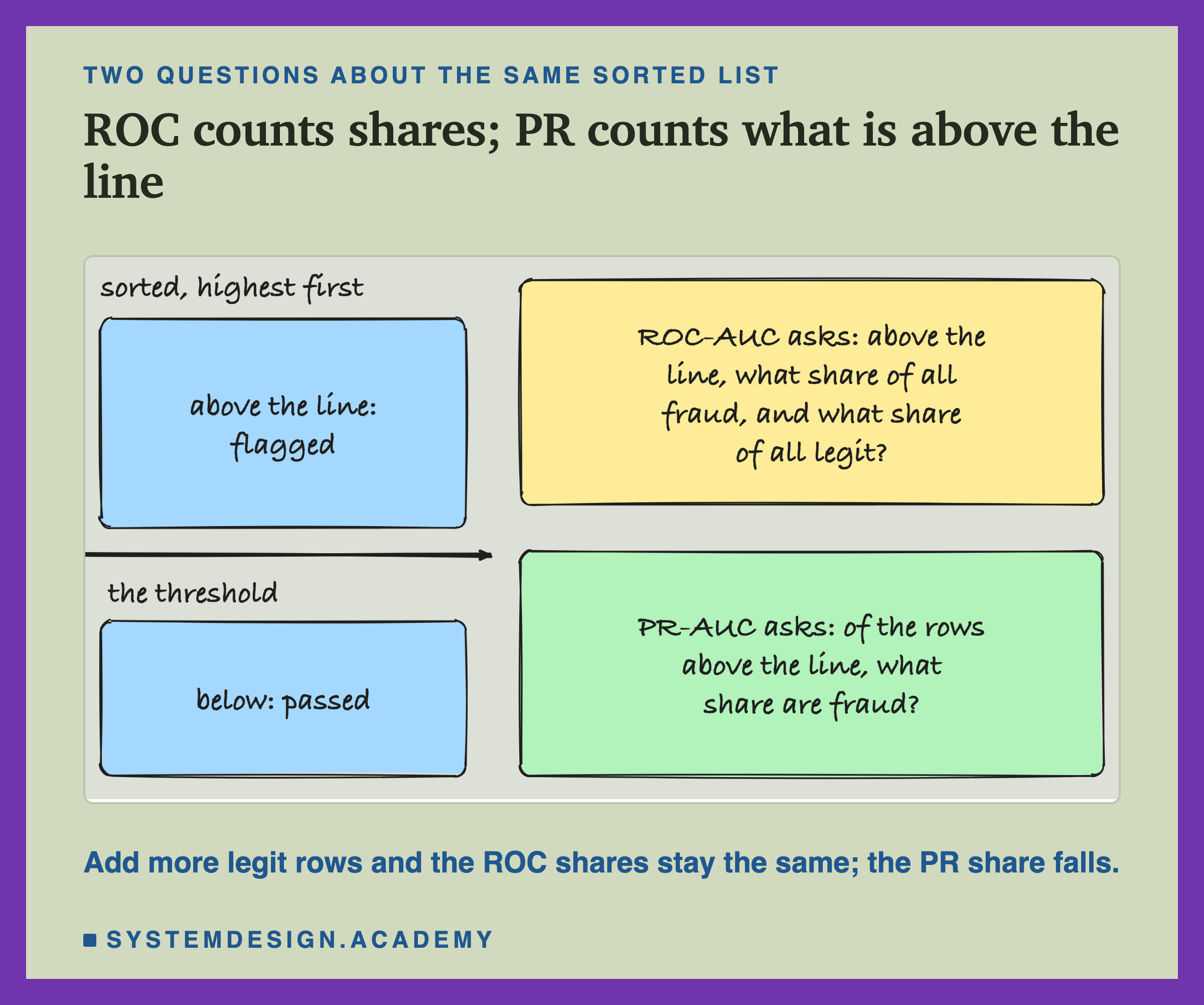
ROC-AUC looks at two shares at every threshold: the share of all frauds above the line, and the share of all legit payments above the line. Its area works out to a simple chance. It is the chance that a random fraud is ranked above a random legit payment. A ranking by coin toss scores 0.5, however rare fraud is.

PR-AUC looks at precision at every threshold: of the payments above the line, the share that are fraud. Here it means scikit-learn's average_precision_score. That sums, over each threshold, the recall gained times the precision there. scikit-learn's page says this "is different from computing the area under the precision-recall curve with the trapezoidal rule", which "can be too optimistic". A ranking by coin toss scores about the fraud share, here 0.0017.

The difference matters. ROC-AUC uses shares of each class on its own, so it does not care how many legit payments there are. PR-AUC counts every false alarm above the line against the frauds above it, so the number of legit payments matters a lot. The next slide measures exactly that.

To see how each number reacts to rarity alone, I kept everything else fixed. For each seed, the model was trained once. Then I scored its same probabilities on four test sets. Each kept all the test frauds and a different number of legit payments, so fraud made up 50, 10 or 1 percent, then the natural 0.17 percent.

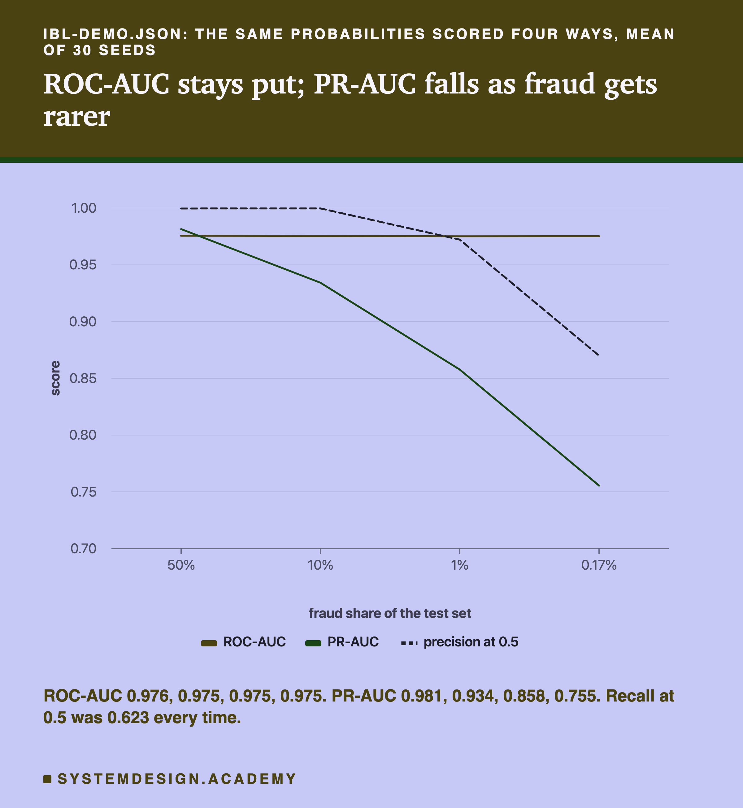
ROC-AUC barely moved: 0.976 with half the test set fraud, 0.975 at the natural 0.17 percent. PR-AUC fell from 0.981 to 0.934, then 0.858, then 0.755. Precision at 0.5 fell from 1.000 to 0.870. Recall at 0.5 stayed at 0.623 every time.

Two of these were certain before the run, and I want to say so plainly. Recall could not move, because the frauds and their probabilities were the same each time. ROC-AUC should not move, because it is built from shares of each class. What the run adds is the size of the fall in PR-AUC on real data, and the check that ROC-AUC really held. After the results, I counted seed by seed. ROC-AUC moved at most 0.007 across the four test sets of any one seed, and PR-AUC fell in all 30 seeds.

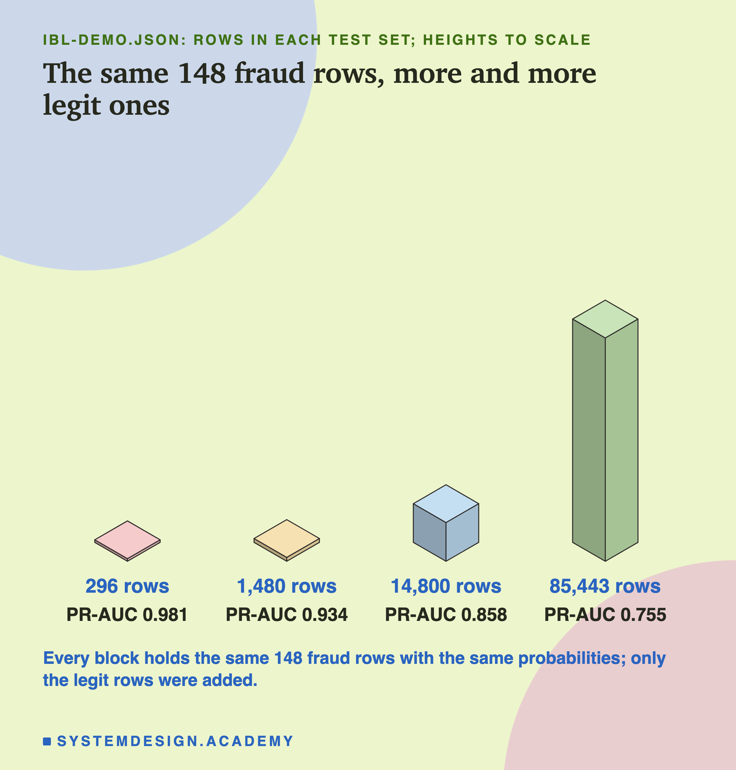
The heights are the number of payments in each test set, to scale. Every block holds the same 148 frauds. Going from left to right only adds legit payments, about 85,000 of them. Some of those get high probabilities, and each one that lands above the line is a false alarm. PR-AUC counts them. ROC-AUC only sees them as a share of all legit payments, which stays about the same.

So which one is right? Both are honest about what they measure. They answer different questions, and the mistake is to read one as if it answered the other.

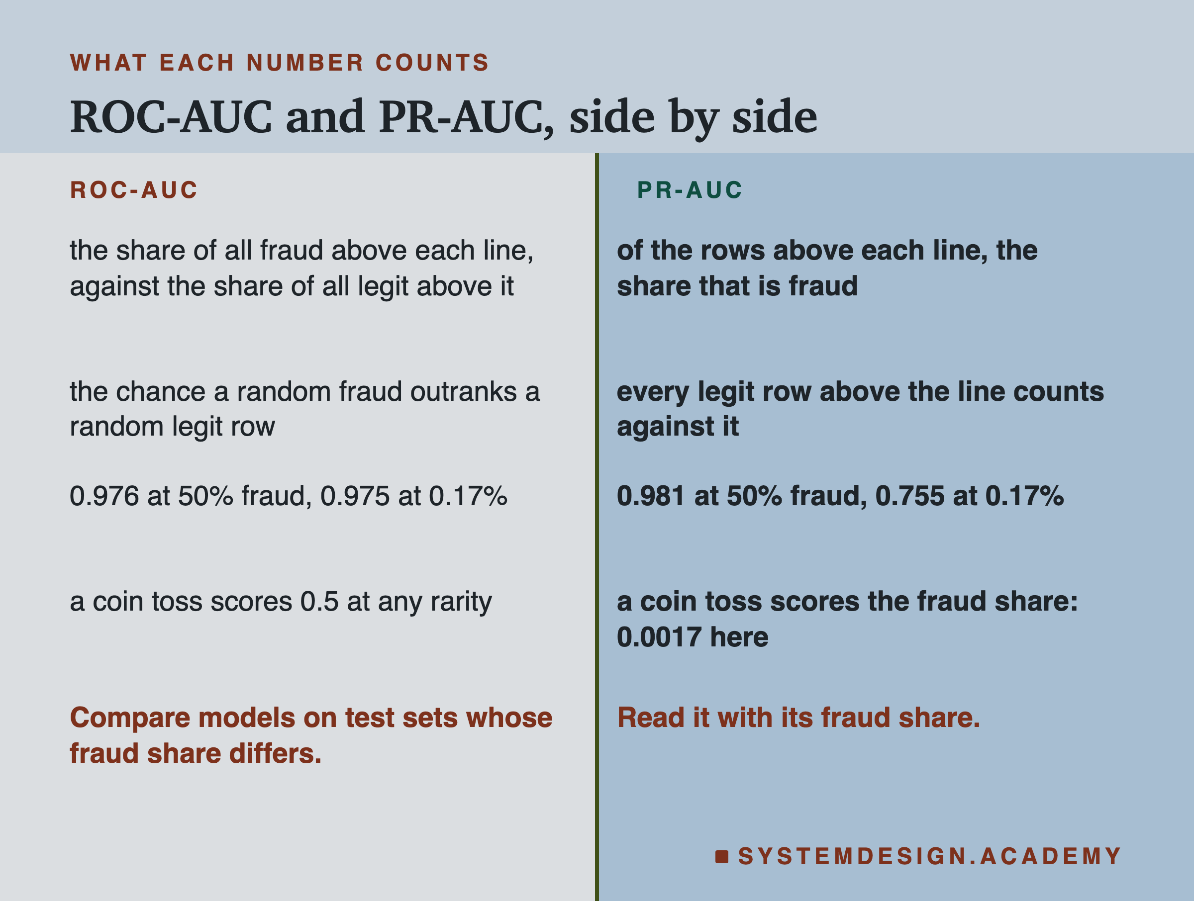
ROC-AUC tells you how well the model ranks, and it is the same whether you test it on rare or common fraud. That makes it good for comparing models on test sets whose fraud share differs. It is bad at telling you what working life will be like at a low rarity.

PR-AUC tells you how clean the top of the list will be at this rarity. If your team can only check 100 payments a day, that is the question you care about. But PR-AUC only means something next to its fraud share. 0.755 at 0.17 percent fraud is far above the coin-toss score of 0.0017. The same 0.755 at 50 percent fraud would be poor.

A 2024 paper by McDermott and others, at the NeurIPS conference, argues that PR-AUC "is not generally superior in cases of class imbalance". It also shows PR-AUC can "unduly favor model improvements in subpopulations with more frequent positive labels": groups of people where the rare class is more common. That can widen unfair gaps between groups. So I read both numbers, and then precision and recall at the threshold I will really use.

Every number so far is a mean over 30 seeds. Here is why one seed would not do.

At the natural rarity, PR-AUC ran from 0.689 on its worst seed to 0.816 on its best. Same data, same model, same code: only the split changed. If I had run one seed and got 0.69, I might have blamed the model. If I had got 0.82, I might have shipped it with too much confidence.

ROC-AUC also moved, from 0.958 to 0.989. Neither spread is a fault in the model. Each test set holds only 148 frauds, and which 148 land there changes the score. With few rare rows, the spread across seeds is part of the answer.

A plain random split can give the test set more or fewer rare rows than its share, just by luck. A stratified split fixes the count. In scikit-learn you pass stratify=y to train_test_split, and the documentation says the data is then "split in a stratified fashion, using this as the class labels".

To see what that buys, I made the problem small on purpose. For each of 100 seeds, I drew 100 frauds and 49,900 legit payments, 0.2 percent fraud. Then I split those same 50,000 rows 80 to 20 twice: once plain, once stratified.

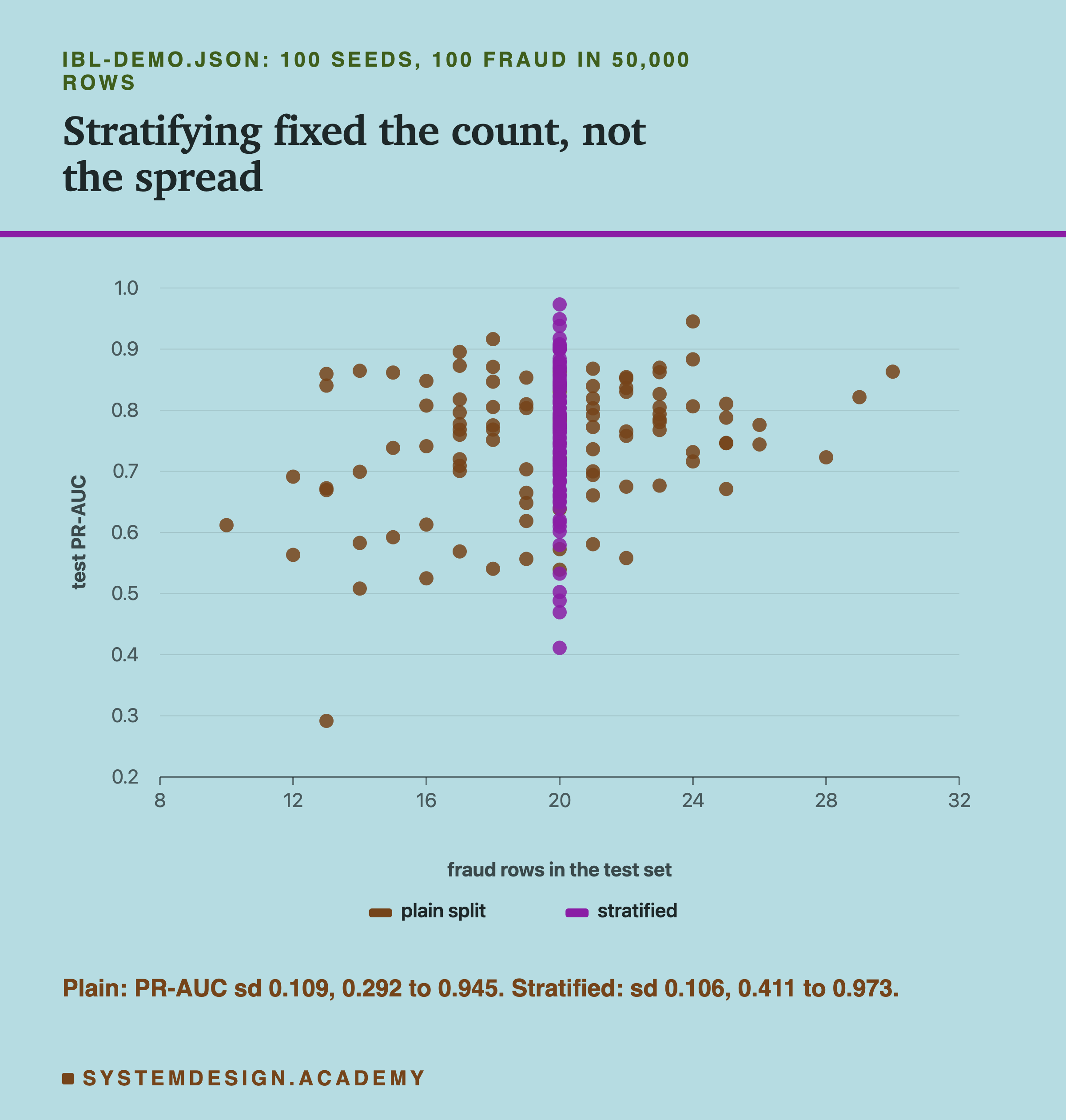
The plain split gave the test set anywhere from 10 to 30 of the 100 frauds. The stratified split gave it exactly 20 every time. That part worked as promised.

What surprised me is the spread of the score. PR-AUC had a standard deviation of 0.109 with plain splits and 0.106 with stratified ones. The standard deviation (sd) is a measure of how far results typically sit from their mean. So stratifying barely narrowed the spread. Recall's spread fell more, from 0.146 to 0.124.

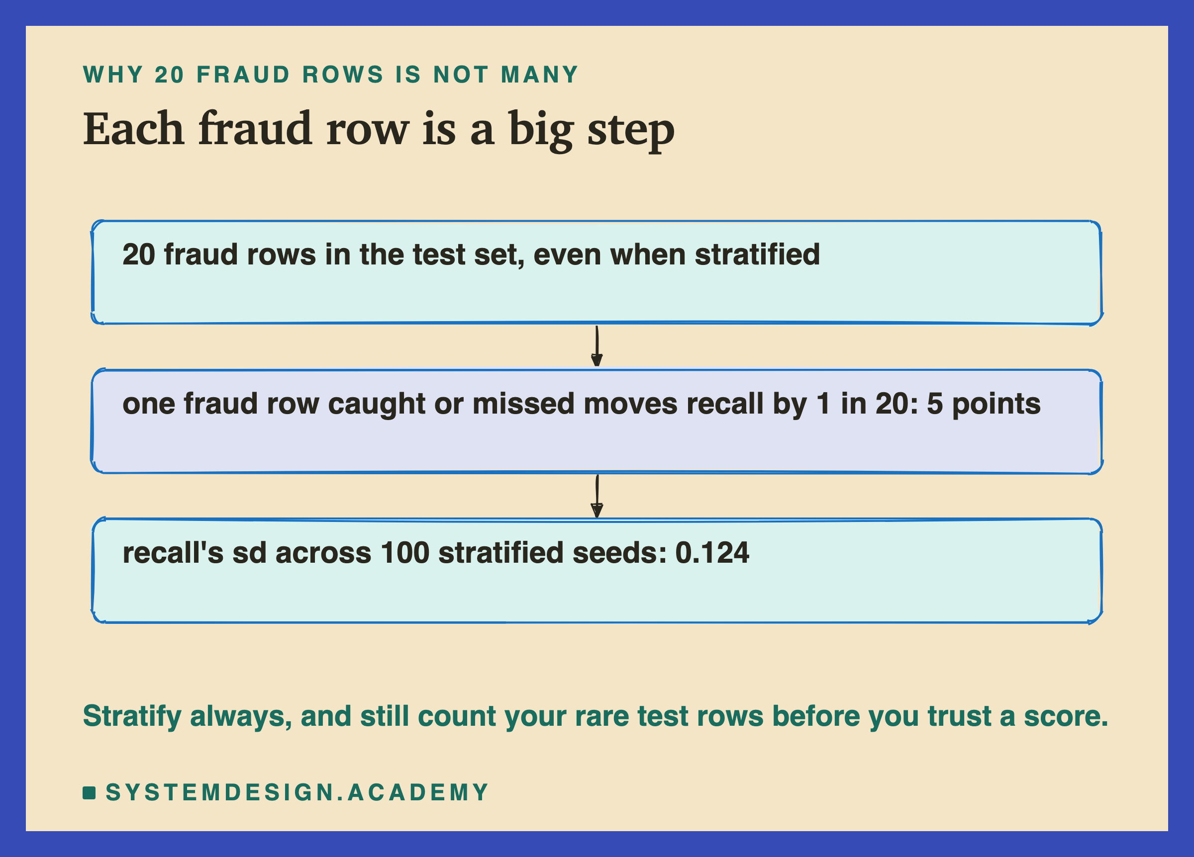
The reason is the small count, not the split. With 20 frauds in the test set, each fraud caught or missed moves recall by 1 in 20, which is 5 points. Which 20 frauds land in the test set changes from seed to seed, stratified or not. So stratify always, because it is free and keeps the count steady. But the split alone does not cure a jumpy score. More rare rows narrow it; more seeds and folds show how wide it is and steady the average. Folds are the parts that cross-validation cuts the data into, explained on the next slide.

A probability is not a decision. The threshold is what turns 0.34 into flag or pass. scikit-learn's documentation says a positive class is predicted "when the conditional probability P(y|X) is greater than 0.5". That 0.5 is a default, not a law.

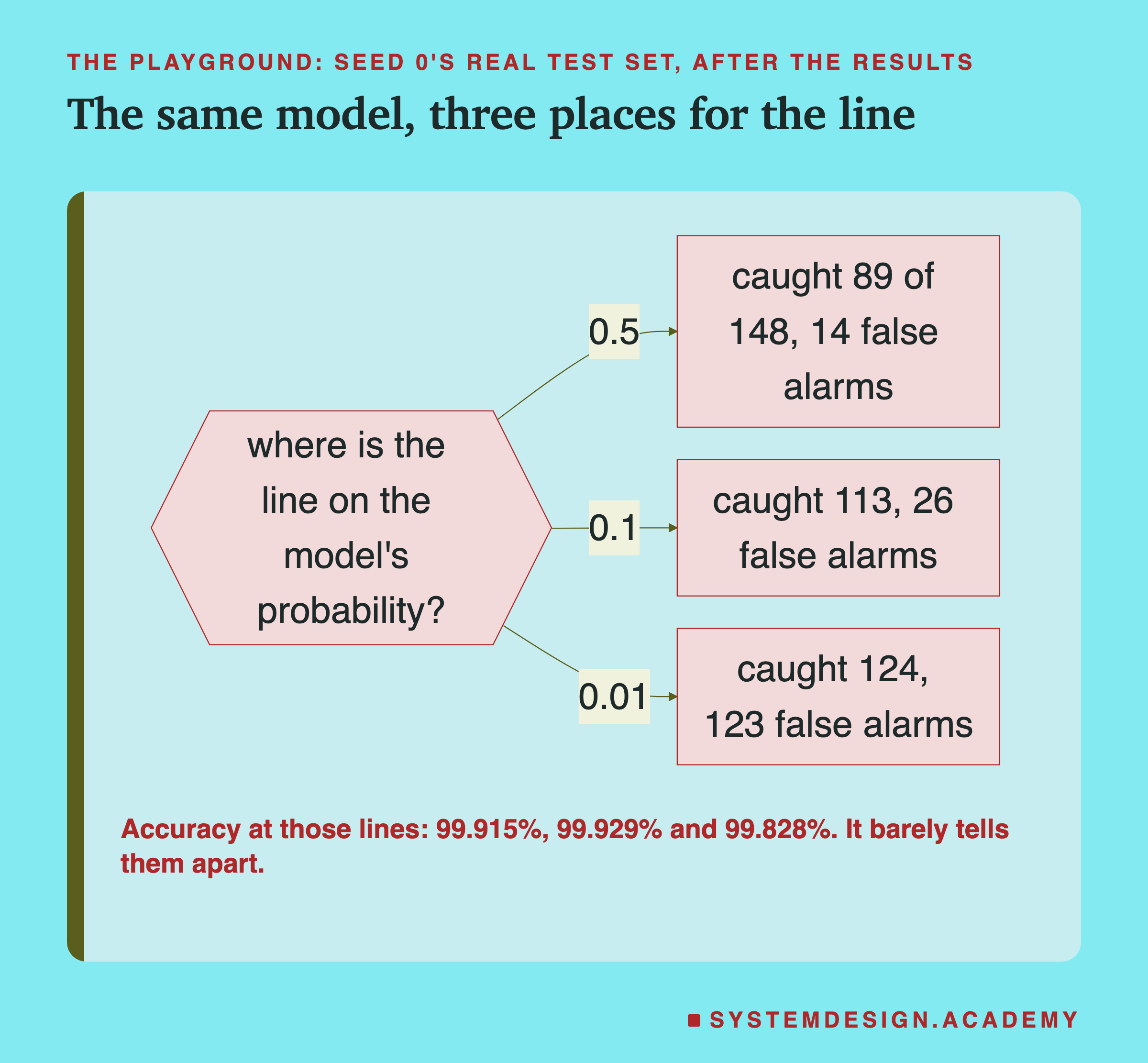
Using the playground further down, I moved the line on seed 0's real test set. These counts came after the results. At 0.5 the model caught 89 frauds with 14 false alarms. At 0.1 it caught 113 with 26. At 0.01 it caught 124 with 123. Accuracy at those three lines was 99.915, 99.929 and 99.828 percent, so it would barely help you choose.

Which line is right depends on cost. If a missed fraud costs a hundred times a false alarm, catching 35 more frauds for 109 more alarms is a good trade. Real fraud systems work this way. Stripe's documentation says its Radar product gives each payment a risk score from 0 to 99, and by default "a score of 75 or above indicates high risk". It also says high-risk payments "are blocked by default", and some plans let a business change that block threshold.

How to choose the line well is the subject of lesson 12. Choose it on a validation set, which is a part of the data kept aside from training for making choices like this one, never on the test set. When the validation set holds only a handful of rare rows, choose it by cross-validation instead. Cross-validation cuts the training data into parts called folds, often 5. It trains on all but one fold, checks on the one left out, and repeats until every fold has had a turn. scikit-learn's TunedThresholdClassifierCV does this. In lesson 12 that did best when rare rows were few.

Rebalancing changes what the model learns from, so that the rare class counts for more. The simplest way is class weights. In scikit-learn it is one argument, class_weight="balanced", which the documentation defines as "n_samples / (n_classes * np.bincount(y))". In words: total rows divided by (2 times the rows in that class).

Lesson 12 measured whether rebalancing beats a well-placed threshold. Here I measured something it described but did not count: what weighting does to the probability itself. On each of the 30 splits, I trained the same model twice, plain and weighted.

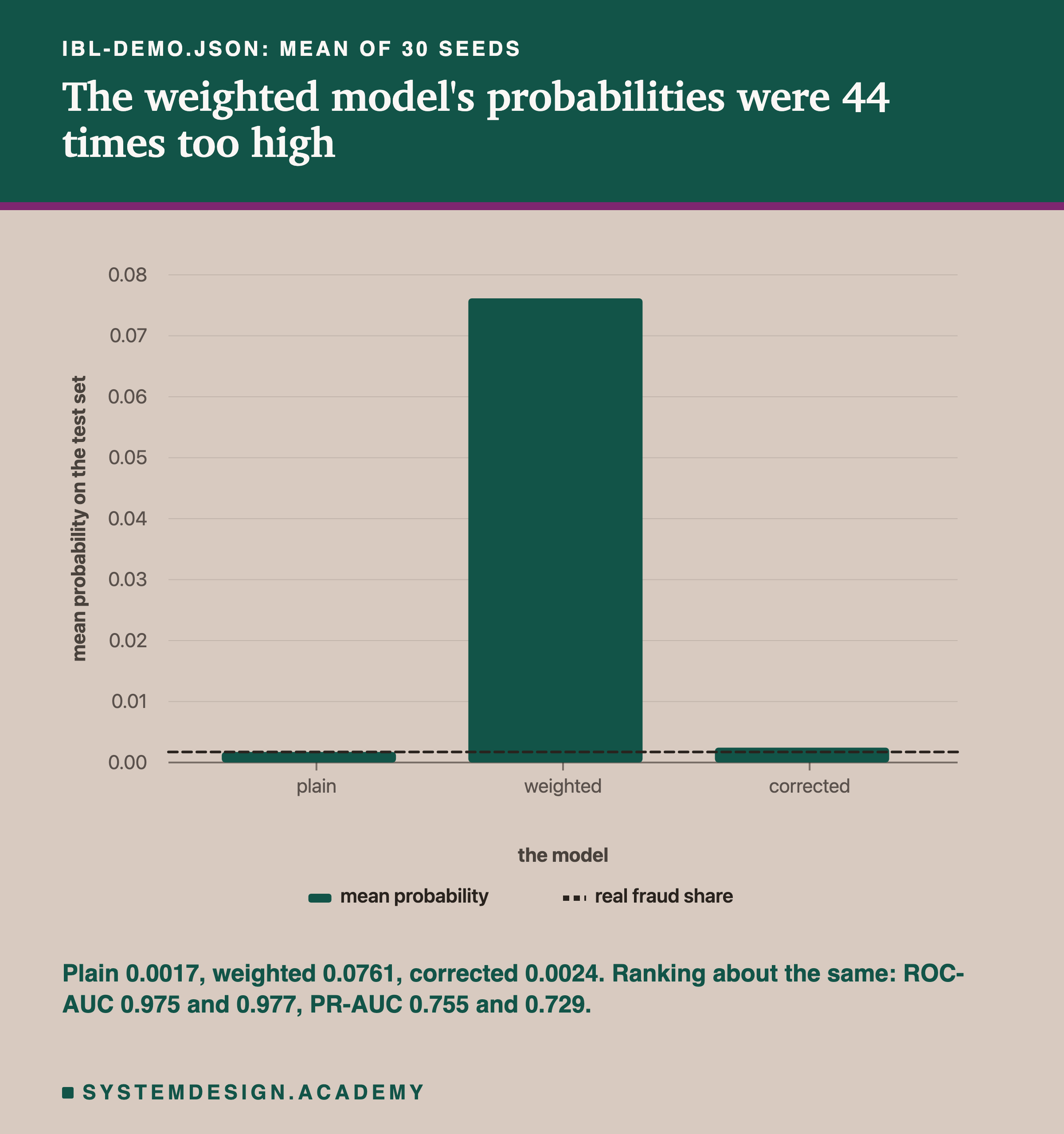
The plain model's average probability on the test set was 0.0017, the same as the real fraud share. The weighted model's was 0.0761, about 44 times too high. Its ranking was about the same: ROC-AUC 0.977 against 0.975. PR-AUC was a little lower, 0.729 against 0.755. After the results I counted seed by seed: PR-AUC was lower with weights in 29 of 30 seeds.

The run also prints a Brier score for each model. It is the average squared gap between each probability and what really happened, 1 or 0, so lower is better. It was 0.00070 for the plain model and 0.02298 for the weighted one.

That matches lesson 12, which found rebalancing barely changed the ranking. It also matches the paper this dataset comes from. Dal Pozzolo and others showed in 2015 that, in theory, undersampling, one kind of rebalancing, shifts a model's probabilities without changing their order. They also noted that a model trained on the smaller, undersampled data gives estimates "subjected to higher variance".

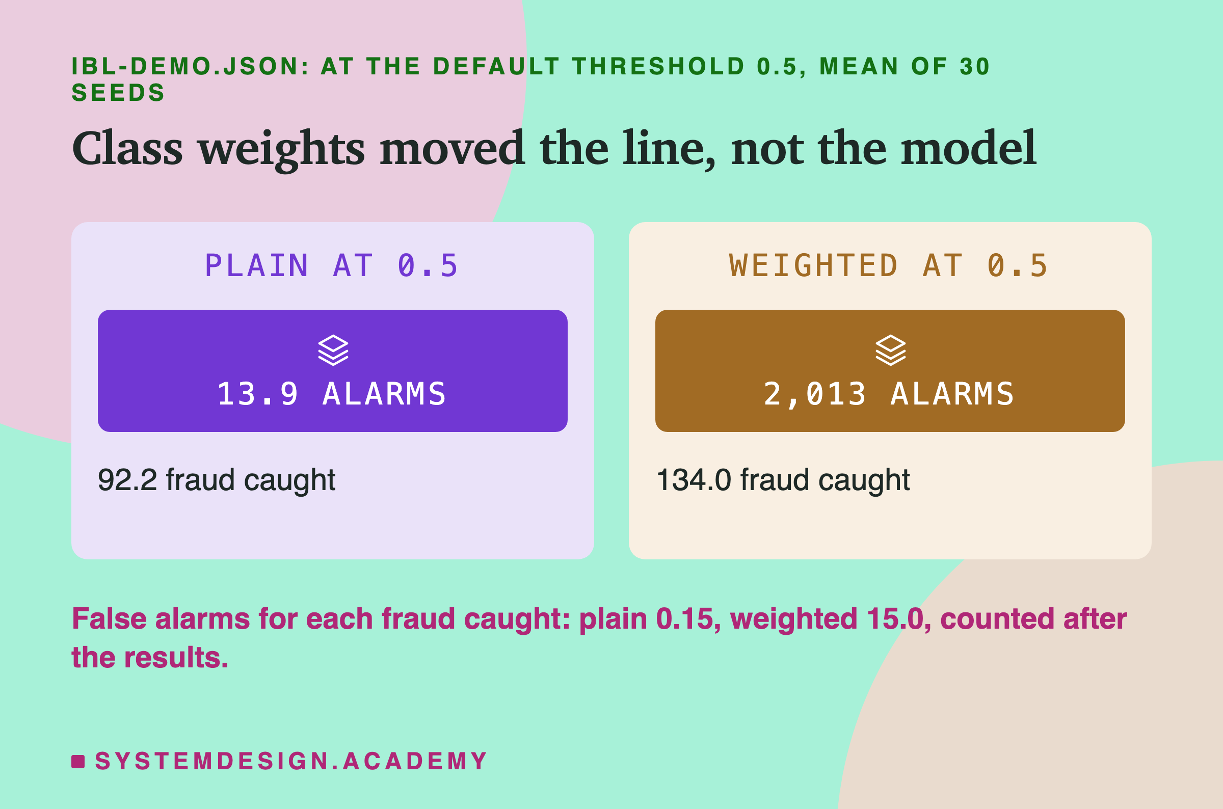
At 0.5, the weighted model caught more frauds, 134.0 against 92.2 on average. It also raised 2,013.0 false alarms against 13.9. That is about 15 false alarms for every fraud it caught, against 0.15 for the plain model. Weighting did not make the model see fraud better. It pushed every probability up, so far more rows crossed the same line. A lower threshold on the plain model flags more rows too, and leaves its probabilities honest.

If anything downstream reads the probability as a real chance, such as a risk score shown to an analyst, a weighted model gives it the wrong number. You can either not rebalance, or correct the number afterwards.

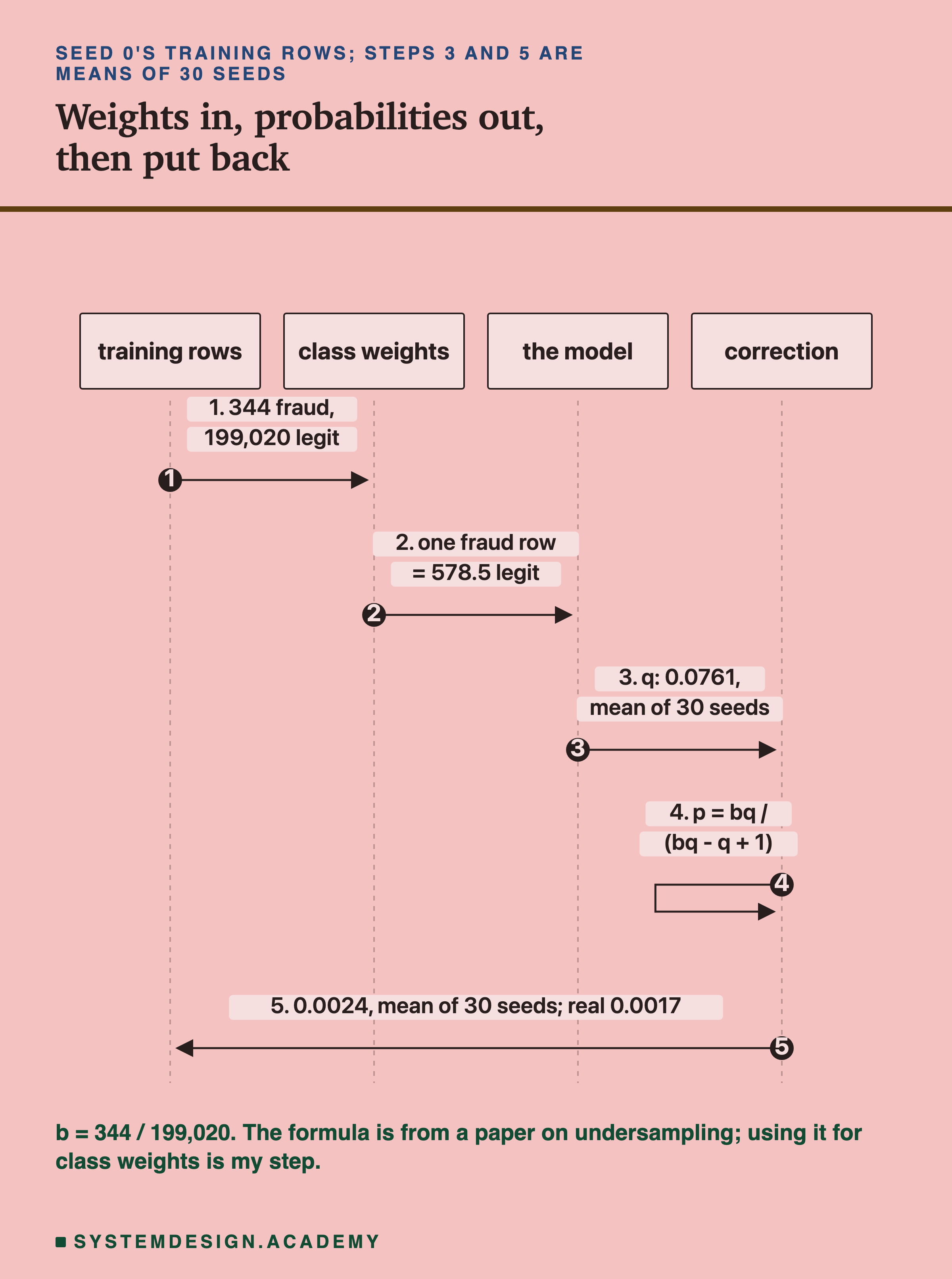
Dal Pozzolo and others give the correction for undersampling, which is throwing away common rows before training. Say q is the model's probability, and b is the share of common rows that were kept. Then the true probability is p = b × q ÷ (b × q − q + 1). Class weights act like keeping a share b of the common rows, with b equal to the rare rows divided by the common rows. Using the formula for weights is my own step, not the paper's.

Worked by hand on seed 0's training rows: 344 frauds and 199,020 legit, so b = 344 ÷ 199,020 = 0.001728. A weighted probability of 0.5 becomes 0.000864 ÷ (0.000864 − 0.5 + 1) = 0.000864 ÷ 0.500864 = 0.0017. So a weighted "50 percent" meant about 0.17 percent.

After the correction, the mean probability was 0.0024, about 1.4 times the real share instead of 44 times. It is closer, not exact. One possible reason is that the model's built-in penalty, called regularisation, acts differently on weighted rows. The correction cannot change the ranking, so its PR-AUC stayed at 0.729. If you need probabilities, the simplest safe choice is still the plain model with a well-placed threshold.

Class weights are one of several tools. Here is what each one does, from its own documentation, and where it fits after the results above and in lesson 12.

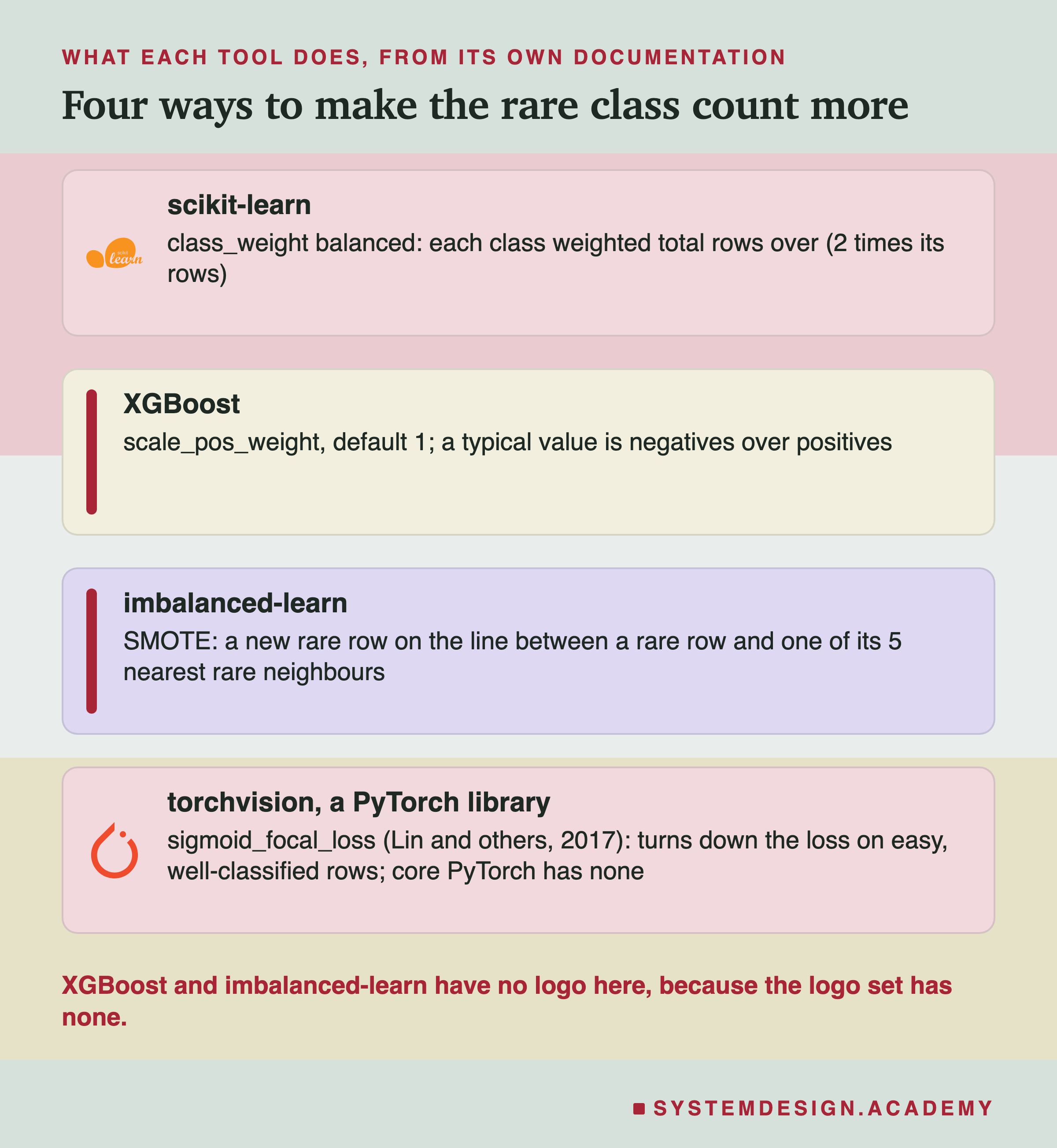
XGBoost is a popular library for boosted trees, which are many small decision trees built one after another, each fixing the last one's mistakes. It has scale_pos_weight. Its documentation says the default is 1, and "a typical value to consider: sum(negative instances) / sum(positive instances)". It does the same job as class weights.

Copying rare rows until the classes are even is called random oversampling. It adds no new information. Copies made before the split also land on both sides of it, which lesson 13 measured as a large leak.

SMOTE, the Synthetic Minority Over-sampling Technique, comes from a 2002 paper by Chawla and others. It makes a new rare row on the straight line between a real rare row and one of its nearest rare neighbours. The imbalanced-learn library looks at 5 neighbours by default. Its documentation warns that "SMOTE might connect inliers and outliers". An outlier is a row far from the others of its class, and an inlier is a typical one. For data with category columns there is SMOTENC, which gives each new row "the most frequent category of the nearest neighbors". I did not run SMOTE here; lesson 12 did.

Undersampling throws away common rows. It makes training faster on huge data, and it shifts probabilities exactly as the correction slide described. Focal loss, from a 2017 paper by Lin and others, is used in deep learning. It "down-weights the loss assigned to well-classified examples", and was built for object detectors where most candidate boxes are background. Core PyTorch has no focal loss, but its torchvision library has , with defaults alpha 0.25 and gamma 2.

The earlier version of this lesson said: start with class weights, add SMOTE if needed, and tune the threshold last. Lesson 12 measured that order and found it backwards. A plain model with its threshold tuned beat every rebalanced model left at 0.5 on its digits data. And choosing the threshold by cross-validation did best when rare rows were few.

This lesson adds two measured reasons to agree. Class weights left the ranking about the same here, with PR-AUC lower in 29 of 30 seeds. And they raised the probabilities about 44 times, which breaks anything that reads them.

So the order I now use is this. Report honest numbers: PR-AUC with its fraud share, ROC-AUC, and precision and recall at a stated threshold. Tune the plain model's threshold on validation data or by cross-validation. Then try rebalancing, give it its own tuned threshold, and keep it only if it beats the plain model. If you keep it and anything reads the probability, correct it.

There are cases where rebalancing may still help. Lesson 12 tested logistic regression only, and so did I. Tree models choose their splits by counting rows, so weighting can change what they learn. Test it on your own model rather than trusting a rule.

Imbalance is half of this lesson's title. The other half is messy data. Real data has gaps, typos, mixed codes and copies. This dataset has no missing values, but it does have copies, and copies matter most at the split.

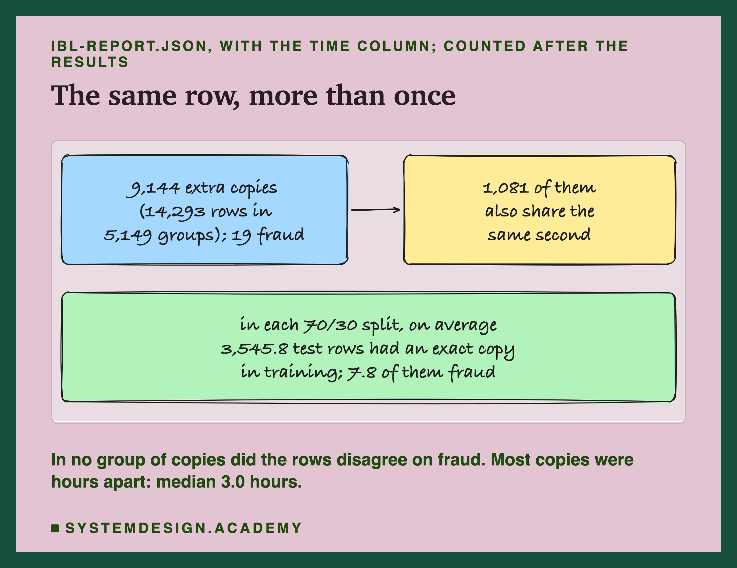
9,144 rows are extra copies of another row in all 29 columns, and 19 of those are fraud. Counted as groups, 14,293 rows sit in 5,149 groups of two or more equal rows. After the results, I read the time column too. Only 1,081 of the copies also share the same second. Inside a group of copies, the rows were a median of 3.0 hours apart, and in no group did they disagree on fraud.

So some of these may be one payment logged twice, and some may be two real payments that look the same. From this data I cannot tell which. What I can measure is the effect on the split. On average, 3,545.8 test rows had an exact copy in training, and 7.8 of them were fraud. A model may have memorised those. So a few of its "test" frauds were not new to it.

The fix depends on what the copies are. If they are the same event logged twice, drop them before the split. If they may be real repeats, keep them but put all copies of a row on the same side of the split. scikit-learn's GroupShuffleSplit does that if you give each group of copies one id, but it does not stratify. When you want both, StratifiedGroupKFold keeps groups apart while it "attempts to return stratified folds". And for data that arrives over time, like fraud, test on later rows than you train on.

This dataset had no gaps, so this slide is general advice, checked against the documentation rather than measured. Lesson 5, on data validation, measured which checks catch a bad batch.

Missing values. Most models cannot take an empty cell, so you fill it, a step called imputation. For a number column, the training median is a common fill. The median is the middle value, so one huge typo cannot drag it the way it drags a mean. For a category column, make "Unknown" its own category with SimpleImputer(strategy="constant", fill_value="Unknown"), rather than the most common value. The fact that a value is missing can carry signal. scikit-learn's add_indicator=True adds a column that says so, which the documentation says "allows a predictive estimator to account for missingness despite imputation".

A column that is mostly empty is mostly guesswork once filled. Dropping it above about half empty is a rule of thumb, not a law.

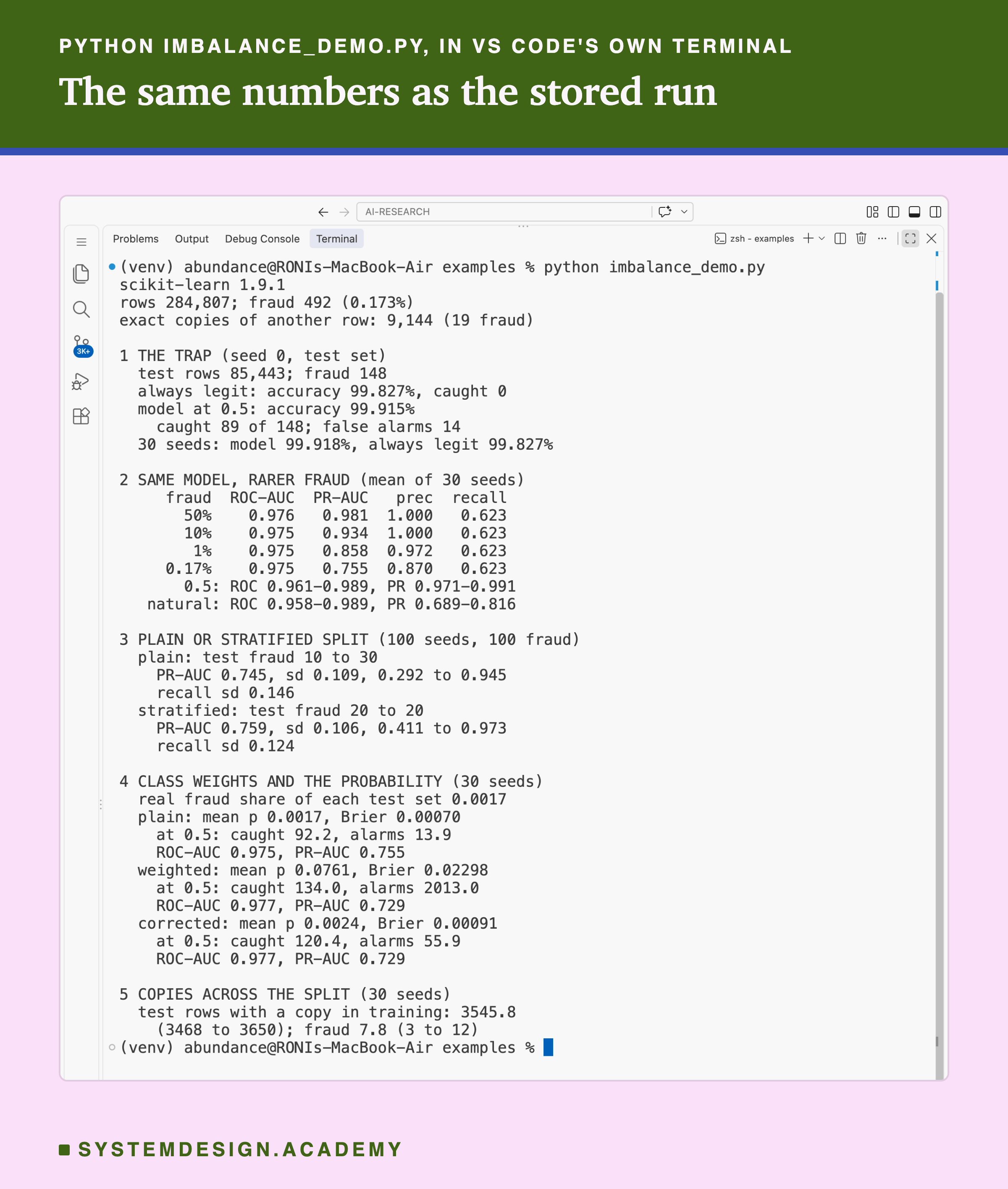
This script is the lab. It downloads the card payments, then runs all five parts. They are the trap, the same model at four rarities, the two kinds of split, class weights, and the copies. It needs no GPU. On my laptop it ran in well under a minute, and it prints no timings.

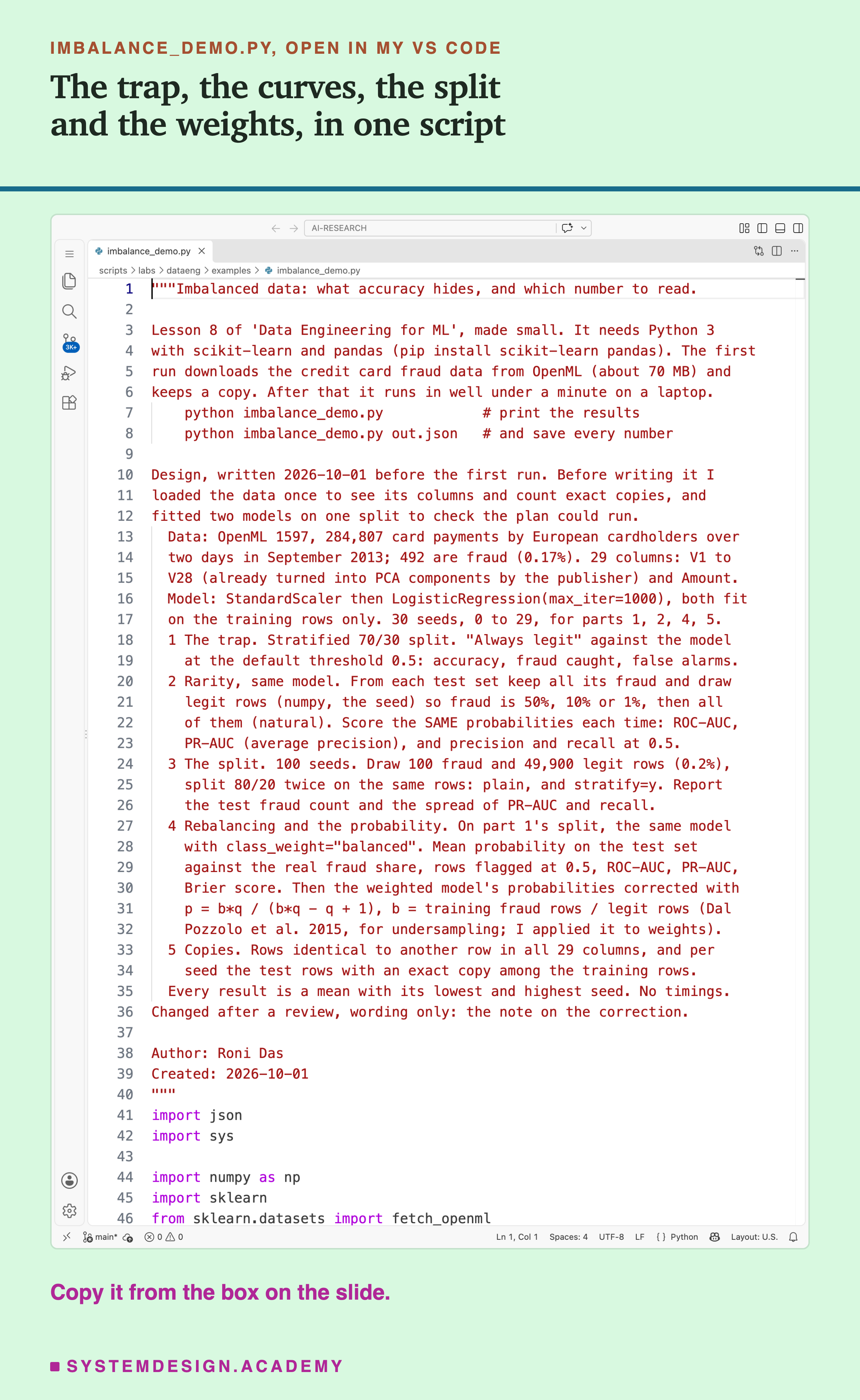
Before you run this lab. You need Python 3 and two libraries: pip install scikit-learn pandas. scikit-learn does the download, the split, the model and the scores, and brings NumPy with it. pandas is what scikit-learn uses to read the downloaded table. The first run downloads the data from OpenML (about 70 MB), so it needs an internet connection once. After that, scikit-learn keeps a copy in a folder in your home directory (scikit_learn_data).

I ran it with scikit-learn 1.9.1 on a Mac. These libraries run on Windows and Linux too, but I have not checked the numbers there. Another version of scikit-learn may give slightly different probabilities, so the first line printed is the version. Give it a file name, python imbalance_demo.py out.json, and it also saves every number. That is how results/ibl-demo.json was made. Two runs gave byte-for-byte the same file.

"""Imbalanced data: what accuracy hides, and which number to read.

Lesson 8 of 'Data Engineering for ML', made small. It needs Python 3
with scikit-learn and pandas (pip install scikit-learn pandas). The first
run downloads the credit card fraud data from OpenML (about 70 MB) and
keeps a copy. After that it runs in well under a minute on a laptop.
    python imbalance_demo.py            # print the results
    python imbalance_demo.py out.json   # and save every number

Design, written 2026-10-01 before the first run. Before writing it I
loaded the data once to see its columns and count exact copies, and
fitted two models on one split to check the plan could run.
  Data: OpenML 1597, 284,807 card payments by European cardholders over
  two days in September 2013; 492 are fraud (0.17%). 29 columns: V1 to
  V28 (already turned into PCA components by the publisher) and Amount.
  Model: StandardScaler then LogisticRegression(max_iter=1000), both fit
  on the training rows only. 30 seeds, 0 to 29, for parts 1, 2, 4, 5.
  1 The trap. Stratified 70/30 split. "Always legit" against the model
    at the default threshold 0.5: accuracy, fraud caught, false alarms.
  2 Rarity, same model. From each test set keep all its fraud and draw
    legit rows (numpy, the seed) so fraud is 50%, 10% or 1%, then all
    of them (natural). Score the SAME probabilities each time: ROC-AUC,
    PR-AUC (average precision), and precision and recall at 0.5.
  3 The split. 100 seeds. Draw 100 fraud and 49,900 legit rows (0.2%),
    split 80/20 twice on the same rows: plain, and stratify=y. Report
    the test fraud count and the spread of PR-AUC and recall.
  4 Rebalancing and the probability. On part 1's split, the same model
    with class_weight="balanced". Mean probability on the test set
    against the real fraud share, rows flagged at 0.5, ROC-AUC, PR-AUC,
    Brier score. Then the weighted model's probabilities corrected with
    p = b*q / (b*q - q + 1), b = training fraud rows / legit rows (Dal
    Pozzolo et al. 2015, for undersampling; I applied it to weights).
  5 Copies. Rows identical to another row in all 29 columns, and per
    seed the test rows with an exact copy among the training rows.
  Every result is a mean with its lowest and highest seed. No timings.
Changed after a review, wording only: the note on the correction.

Author: Roni Das
Created: 2026-10-01
"""
import json
import sys

import numpy as np
import sklearn
from sklearn.datasets import fetch_openml
from sklearn.linear_model import LogisticRegression
from sklearn.metrics import (average_precision_score, brier_score_loss,
                             roc_auc_score)
from sklearn.model_selection import train_test_split
from sklearn.pipeline import make_pipeline
from sklearn.preprocessing import StandardScaler

SEEDS = range(30)
SPLIT_SEEDS = range(100)
SHARES = [0.5, 0.1, 0.01]          # fraud share of the test set; then all


def model(weights=None):
    return make_pipeline(StandardScaler(), LogisticRegression(
        max_iter=1000, class_weight=weights))


def at_half(y, p):
    """Counts at the default threshold 0.5."""
    flag = p >= 0.5
    caught = int((flag & (y == 1)).sum())
    alarms = int((flag & (y == 0)).sum())
    return {"caught": caught, "alarms": alarms,
            "fraud": int(y.sum()), "rows": len(y),
            "accuracy": float((flag == (y == 1)).mean()),
            "recall": caught / max(1, int(y.sum())),
            "precision": caught / max(1, caught + alarms)}


def scores(y, p):
    return {"roc_auc": float(roc_auc_score(y, p)),
            "pr_auc": float(average_precision_score(y, p)),
            **at_half(y, p)}


def spread(xs):
    xs = np.asarray(xs, float)
    return {"mean": float(xs.mean()), "min": float(xs.min()),
            "max": float(xs.max()), "sd": float(xs.std())}


# ── the data ──
d = fetch_openml(data_id=1597, as_frame=True, parser="auto")
X = d.data.to_numpy(float)
y = (d.target.astype(str) == "1").to_numpy().astype(int)
# row_key: the same number for rows equal in all 29 columns
_, first, row_key = np.unique(X, axis=0, return_index=True,
                              return_inverse=True)
row_key = row_key.ravel()
print(f"scikit-learn {sklearn.__version__}")
print(f"rows {len(y):,}; fraud {y.sum()} ({y.mean():.3%})")
out = {"version": sklearn.__version__, "rows": len(y),
       "fraud": int(y.sum()), "copies": len(y) - len(first),
       "fraud_copies": int(y.sum() - y[first].sum())}
print(f"exact copies of another row: {out['copies']:,}"
      f" ({out['fraud_copies']} fraud)")

runs = []
for seed in SEEDS:
    tr, te = train_test_split(np.arange(len(y)), test_size=0.3,
                              stratify=y, random_state=seed)
    plain = model().fit(X[tr], y[tr])
    weighted = model("balanced").fit(X[tr], y[tr])
    p, q = plain.predict_proba(X[te])[:, 1], weighted.predict_proba(X[te])[:, 1]
    yt = y[te]
    # 2: the same probabilities, on test sets of four fraud shares
    rng = np.random.default_rng(seed)
    fraud, legit = np.flatnonzero(yt == 1), np.flatnonzero(yt == 0)
    rare = {}
    for s in SHARES:
        keep = rng.choice(legit, round(len(fraud) * (1 - s) / s), replace=False)
        idx = np.concatenate([fraud, keep])
        rare[str(s)] = scores(yt[idx], p[idx])
    rare["natural"] = scores(yt, p)
    # 4: the weighted model's probabilities, corrected for the weights
    b = y[tr].sum() / (len(tr) - y[tr].sum())
    fixed = b * q / (b * q - q + 1)
    prob = {}
    for name, v in (("plain", p), ("weighted", q), ("corrected", fixed)):
        prob[name] = {"mean_p": float(v.mean()),
                      "brier": float(brier_score_loss(yt, v)), **scores(yt, v)}
    # 5: test rows with an exact copy among the training rows
    twin = np.isin(row_key[te], row_key[tr])
    runs.append({"seed": seed, "train_fraud": int(y[tr].sum()),
                 "base_accuracy": float(1 - yt.mean()), "rare": rare,
                 "prob": prob, "twins": int(twin.sum()),
                 "fraud_twins": int((twin & (yt == 1)).sum())})
out["runs"] = runs

# 3: plain and stratified splits of the same 50,000 rows
splits = {"plain": [], "stratified": []}
for seed in SPLIT_SEEDS:
    rng = np.random.default_rng(1000 + seed)
    idx = np.concatenate([
        rng.choice(np.flatnonzero(y == 1), 100, replace=False),
        rng.choice(np.flatnonzero(y == 0), 49_900, replace=False)])
    for kind in splits:
        tr, te = train_test_split(idx, test_size=0.2, random_state=seed,
                                  stratify=y[idx] if kind != "plain" else None)
        m = model().fit(X[tr], y[tr])
        r = scores(y[te], m.predict_proba(X[te])[:, 1])
        splits[kind].append({"fraud": r["fraud"], "pr_auc": r["pr_auc"],
                             "recall": r["recall"]})
out["splits"] = splits

# ── what it found ──
R0 = runs[0]["rare"]["natural"]
print("\n1 THE TRAP (seed 0, test set)")
print(f"  test rows {R0['rows']:,}; fraud {R0['fraud']}")
print(f"  always legit: accuracy {runs[0]['base_accuracy']:.3%}, caught 0")
print(f"  model at 0.5: accuracy {R0['accuracy']:.3%}")
print(f"    caught {R0['caught']} of {R0['fraud']}; "
      f"false alarms {R0['alarms']}")
acc = spread([r["rare"]["natural"]["accuracy"] for r in runs])
base = spread([r["base_accuracy"] for r in runs])
print(f"  30 seeds: model {acc['mean']:.3%}, always legit {base['mean']:.3%}")

print("\n2 SAME MODEL, RARER FRAUD (mean of 30 seeds)")
print(f"  {'fraud':>8}{'ROC-AUC':>9}{'PR-AUC':>8}{'prec':>7}{'recall':>8}")
summary = {}
for k in [str(s) for s in SHARES] + ["natural"]:
    summary[k] = {m: spread([r["rare"][k][m] for r in runs])
                  for m in ("roc_auc", "pr_auc", "precision", "recall",
                            "alarms", "rows")}
    share = "0.17%" if k == "natural" else f"{float(k):.0%}"
    s = summary[k]
    print(f"  {share:>8}{s['roc_auc']['mean']:9.3f}{s['pr_auc']['mean']:8.3f}"
          f"{s['precision']['mean']:7.3f}{s['recall']['mean']:8.3f}")
for k in ("0.5", "natural"):
    a, b = summary[k]["roc_auc"], summary[k]["pr_auc"]
    print(f"  {k:>8}: ROC {a['min']:.3f}-{a['max']:.3f},"
          f" PR {b['min']:.3f}-{b['max']:.3f}")
out["rare_summary"] = summary

print("\n3 PLAIN OR STRATIFIED SPLIT (100 seeds, 100 fraud)")
split_summary = {}
for kind, rows in splits.items():
    f = spread([r["fraud"] for r in rows])
    a = spread([r["pr_auc"] for r in rows])
    c = spread([r["recall"] for r in rows])
    split_summary[kind] = {"fraud": f, "pr_auc": a, "recall": c}
    print(f"  {kind}: test fraud {f['min']:.0f} to {f['max']:.0f}")
    print(f"    PR-AUC {a['mean']:.3f}, sd {a['sd']:.3f},"
          f" {a['min']:.3f} to {a['max']:.3f}")
    print(f"    recall sd {c['sd']:.3f}")
out["split_summary"] = split_summary

print("\n4 CLASS WEIGHTS AND THE PROBABILITY (30 seeds)")
print(f"  real fraud share of each test set {1 - base['mean']:.4f}")
prob_summary = {}
for name in ("plain", "weighted", "corrected"):
    s = {m: spread([r["prob"][name][m] for r in runs])
         for m in ("mean_p", "brier", "roc_auc", "pr_auc", "caught",
                   "alarms", "precision", "recall")}
    prob_summary[name] = s
    print(f"  {name}: mean p {s['mean_p']['mean']:.4f},"
          f" Brier {s['brier']['mean']:.5f}")
    print(f"    at 0.5: caught {s['caught']['mean']:.1f},"
          f" alarms {s['alarms']['mean']:.1f}")
    print(f"    ROC-AUC {s['roc_auc']['mean']:.3f},"
          f" PR-AUC {s['pr_auc']['mean']:.3f}")
out["prob_summary"] = prob_summary

print("\n5 COPIES ACROSS THE SPLIT (30 seeds)")
t, ft = spread([r["twins"] for r in runs]), spread([r["fraud_twins"] for r in runs])
print(f"  test rows with a copy in training: {t['mean']:.1f}")
print(f"    ({t['min']:.0f} to {t['max']:.0f}); fraud {ft['mean']:.1f}"
      f" ({ft['min']:.0f} to {ft['max']:.0f})")
out["twin_summary"] = {"rows": t, "fraud": ft}

if len(sys.argv) > 1:
    json.dump(out, open(sys.argv[1], "w"), indent=1)

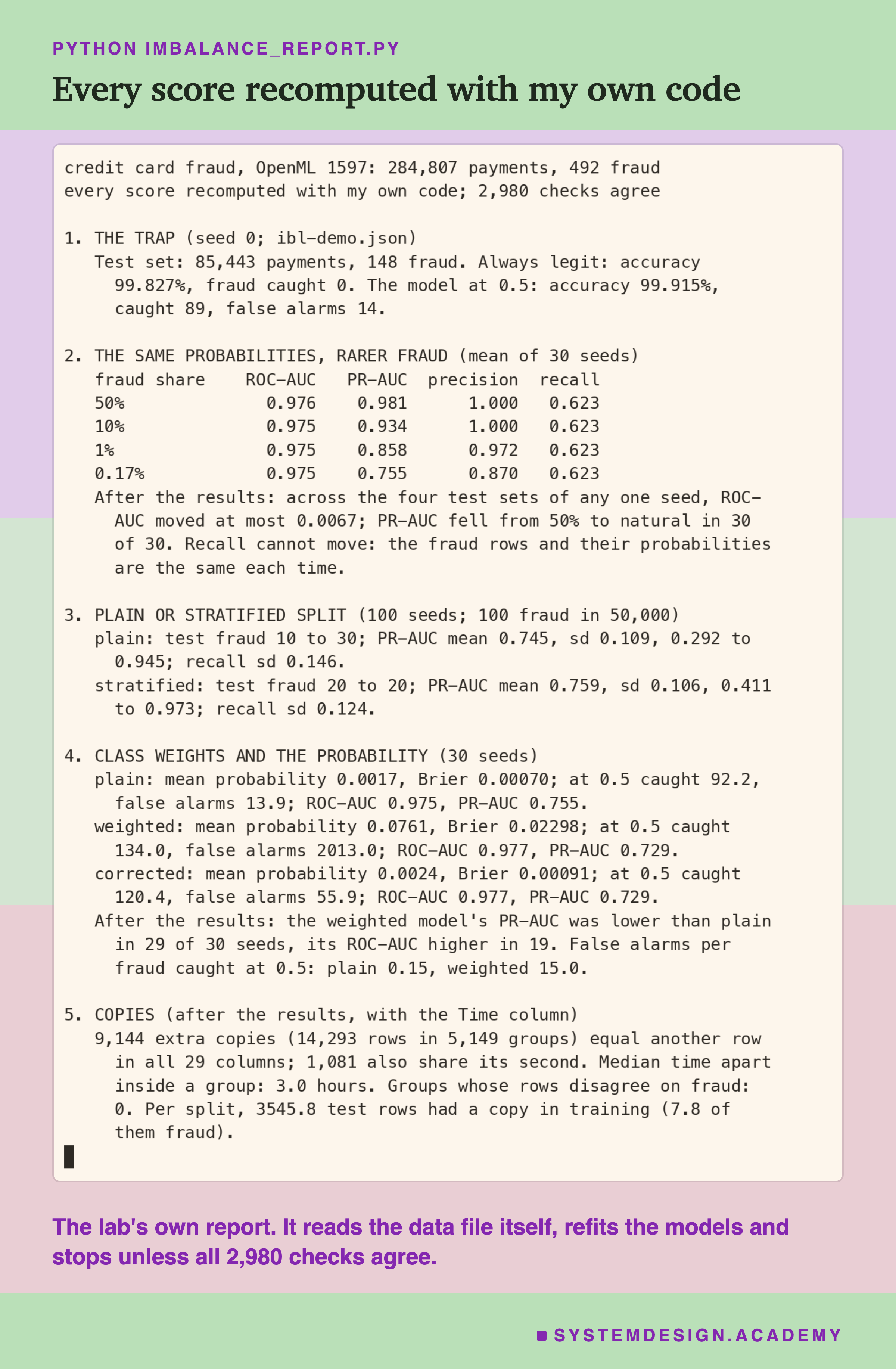
The report lives in scripts/labs/dataeng/imbalance_report.py. It does not trust the demo's code for anything it can redo another way. It reads the downloaded data file itself, keeps the time column, and checks that the other 29 columns match. It fits the same models on the same splits, because the models must be the same. Then it computes every score with its own code: ROC-AUC from ranks, PR-AUC from its formula, the Brier score, the counts at 0.5, and the copies with pandas.

It covers all 30 seeds, all four test sets, all three versions of the probability and all 200 split runs. Every number must come back within one part in a billion. 2,980 checks agreed. It stops at the first one that does not.

Its json mode writes results/ibl-report.json, which the figures read. Its demo mode checks the demo's printed run line by line. Its box mode writes the playground on the next slide and checks it.

What came when: the demo's design, in its docstring, came before any run, and nothing in the demo changed after its first run. Four things came after I saw the results, and the report's docstring lists them. They are the copies with the time column, two sets of seed-by-seed counts, and the false alarms per fraud caught. The thresholds 0.1 and 0.01 on the dial slide came from the playground, also after.

This box holds seed 0's real test set, as the plain model scored it. It has each fraud payment's probability, and how many legit payments scored at or above each threshold on a fixed list. It has no model and no payment data. It runs in your browser.

As it is, the box prints the trap. Always legit scores 99.827 percent and catches 0. The model at 0.5 catches 89 of 148 with 14 false alarms. The report checked those counts at every threshold on the list against the real data.

Then try THRESHOLD = 0.1 and THRESHOLD = 0.01, and watch accuracy barely move while the catches and alarms change a lot. Then set LEGIT_KEPT = 0.01, which keeps about 1 legit payment in 100, so fraud becomes about 15 percent of the test set. Recall stays the same and precision jumps: the rarity slide, on one seed. With LEGIT_KEPT below 1, the false alarms are the expected share of the real count, not a new draw.

The data. fetch_openml(data_id=1597) downloads the payments once and reads the local copy after that. X holds the 29 columns as numbers, and y is 1 for fraud and 0 for legit. np.unique gives every row a number that is the same for exact copies, called row_key.

model. One function builds the pipeline: StandardScaler then LogisticRegression(max_iter=1000), with class_weight either off or "balanced". A pipeline is a chain of steps that is fitted as one, so the scaler only ever learns from the rows the model trains on.

at_half, scores, spread. at_half counts catches, false alarms, accuracy, precision and recall at 0.5. scores adds ROC-AUC and PR-AUC. spread turns a list of 30 or 100 results into a mean, a lowest, a highest and a standard deviation.

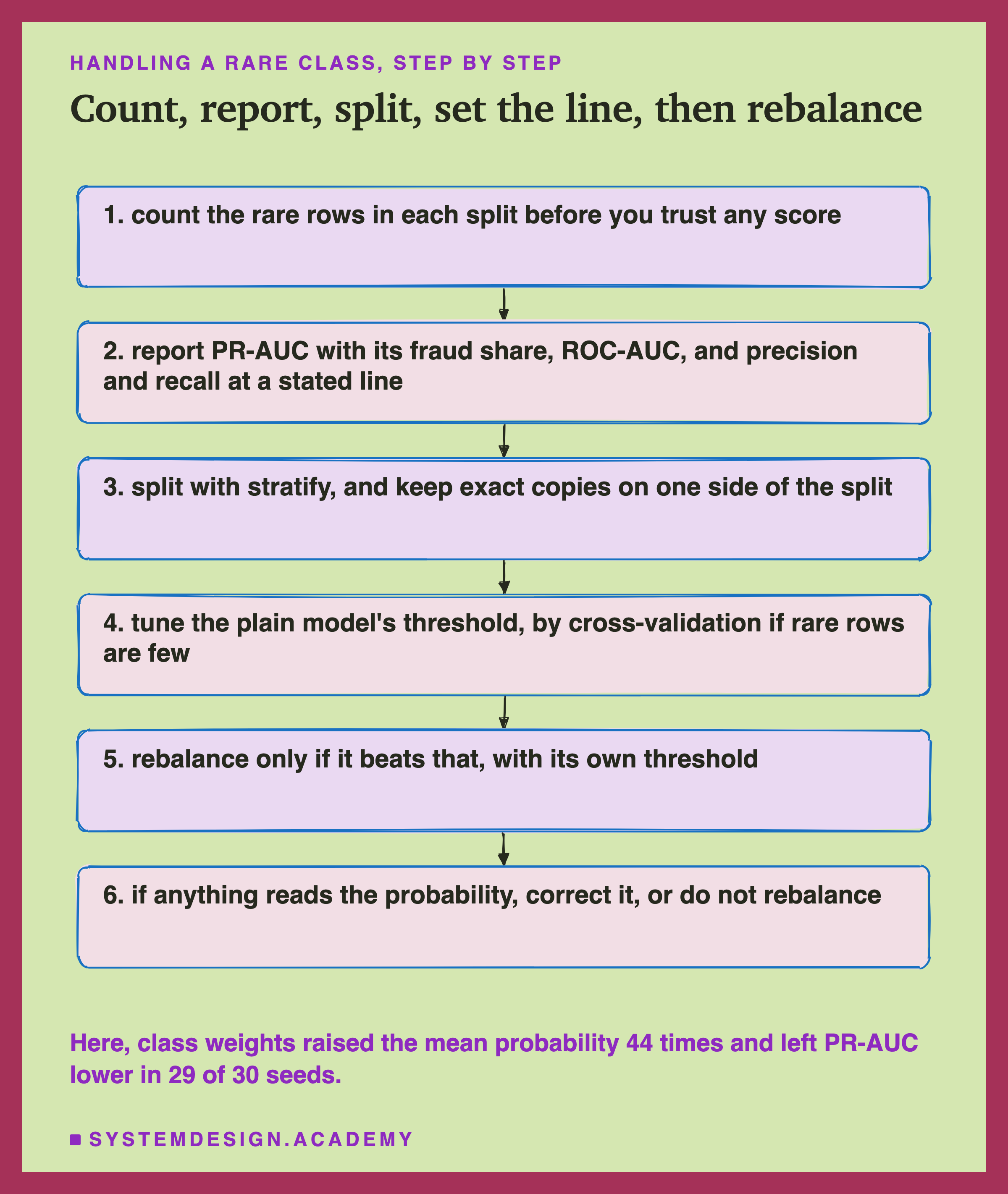
Count the rare rows in each split. Before you trust a score, know how many rare rows it was measured on. Here 148 frauds per test set still left PR-AUC ranging from 0.689 to 0.816 across seeds.

Report the right numbers. PR-AUC with its fraud share, ROC-AUC, and precision and recall at the threshold you will really use. Never accuracy alone.

Split with stratify, and mind the copies. Stratifying is free. Keep exact copies on one side of the split, or drop them if they are the same event twice; StratifiedGroupKFold does both jobs at once. For data that arrives over time, like fraud, test on later rows than you train on.

Tune the plain model's threshold. On validation data, or by cross-validation when rare rows are few. Set it by the cost of each kind of mistake.

Rebalance only if it earns it. Give the rebalanced model its own tuned threshold and keep it only if it beats step 4.

Keep the probabilities honest. If a person or a system reads the number as a chance, correct a rebalanced model's output, or do not rebalance.

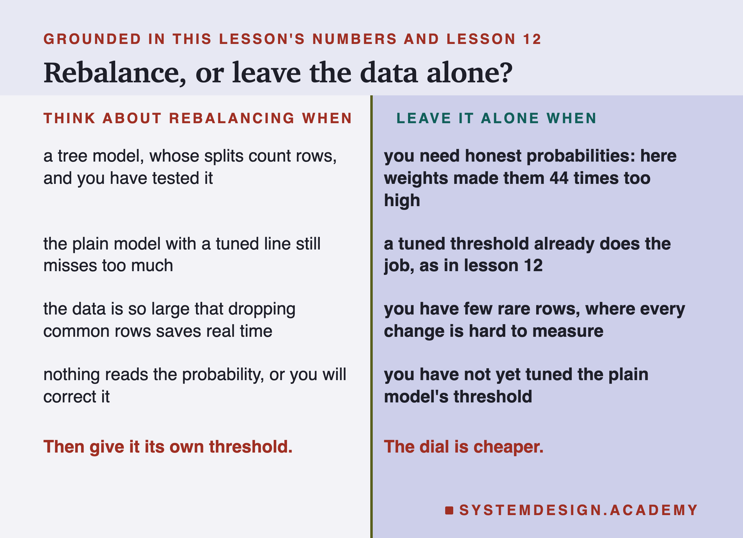
Think about rebalancing when you use a tree model and have tested the effect, because trees choose splits by counting rows. Also when the plain model with a tuned threshold still misses too much, or when the data is so large that dropping common rows saves real time.

Leave it alone when you need honest probabilities, or when a tuned threshold already does the job. Also leave it when you have so few rare rows that any change is hard to measure. And always leave it alone until you have tuned the plain model's threshold, so you know the score it has to beat.

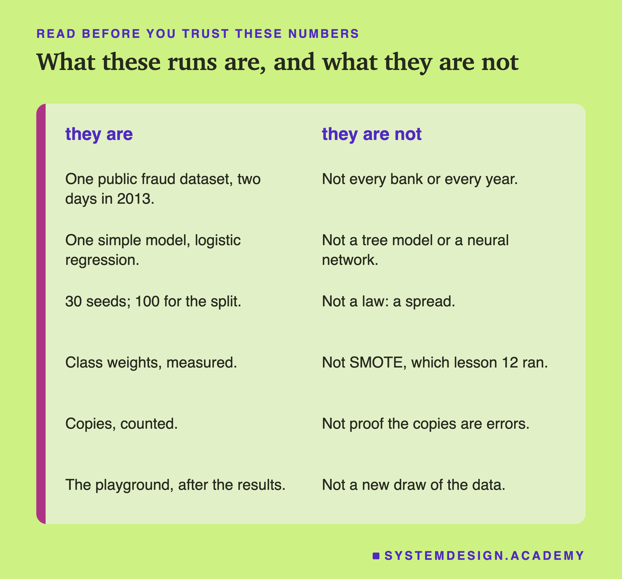
One dataset, two days. Fraud patterns change from bank to bank and year to year. The size of the PR-AUC fall depends on how well the model separates the classes, so another dataset will give other numbers. The direction, ROC-AUC steady and PR-AUC falling, follows from how the two are built.

Random splits, not time. The payments cover two days, and I split them at random. A real fraud system is trained on the past and used on the future, so test on later rows than you train on. I did not measure a split by time, so I cannot say how much these scores would change.

One kind of model. Logistic regression only, with one setting for its built-in penalty. Trees and neural networks may react to class weights differently.

What came after the results. The copies with the time column, the seed-by-seed counts, the false alarms per catch, and the thresholds tried in the playground all came after I saw the results.

The correction was borrowed. The formula comes from a paper on undersampling. Applying it to class weights is my step, and here it got the mean probability within 1.4 times of the real share, not exactly onto it.

Take the model your team runs today and ask the first question: how many rare rows are in the test set behind its score? If the honest answer is "a few dozen", treat its score as a range, not a number.

Then check whether it was rebalanced, and whether anything downstream reads its probability as a real chance. Here, class weights made that number 44 times too high.

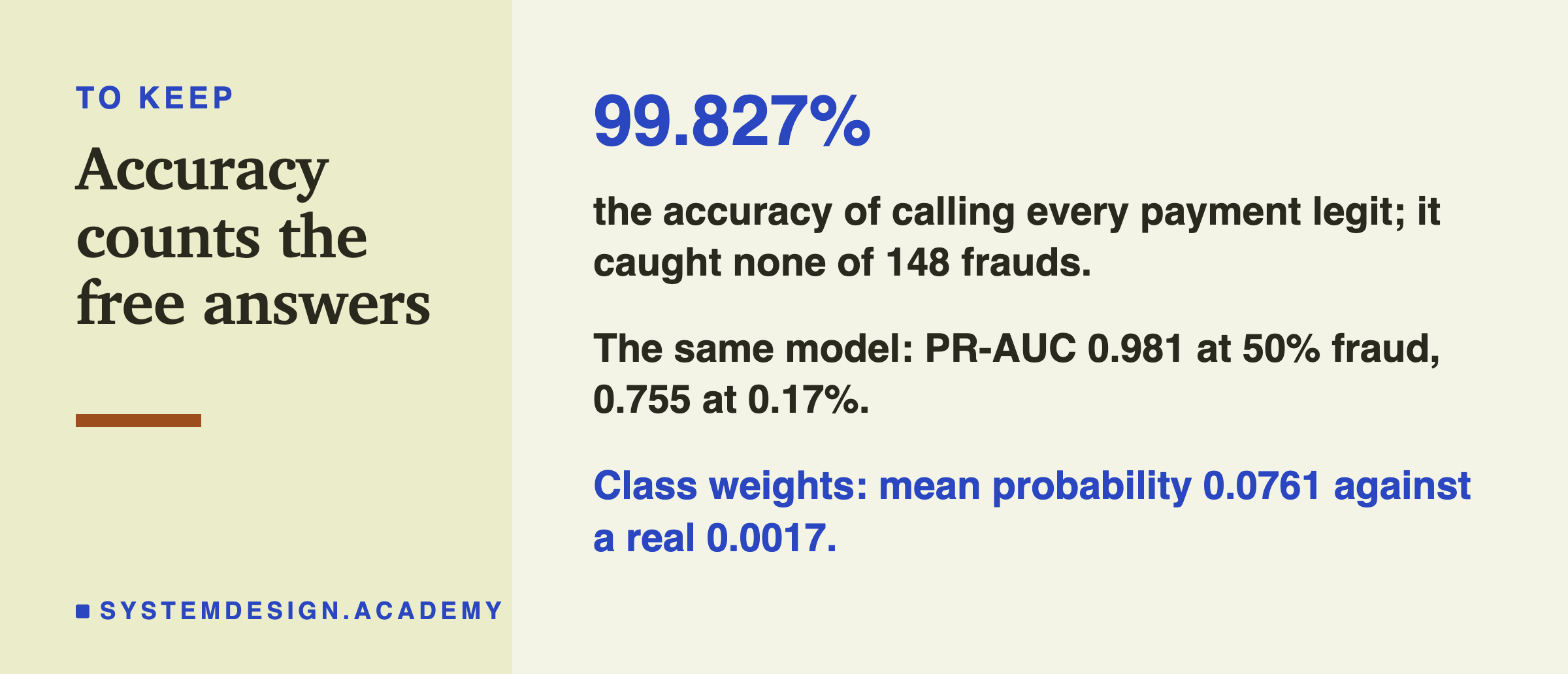
The card keeps the lesson's three numbers. Calling every payment legit scored 99.827 percent and caught nothing. The same model's PR-AUC was 0.981 or 0.755, depending only on how rare fraud was in the test set. And class weights moved the mean probability from the real 0.0017 to 0.0761.

The next lesson in this chapter is about synthetic data: when made-up rows can help, and how to check that they do.