Imagine you want to hire someone to tell you tomorrow's weather. You have a diary that a neighbour kept for two years: every day, the temperature, the rain, the wind. You want to test each person who applies for the job, so you tear out some pages at random and ask them to fill in what those days were like.

One applicant does very well. She opens the diary at a missing Tuesday in October. The rest of that October is still there, so she can see what kind of month it was: warm or cold, wet or dry. She writes something that fits, and she is almost always close. It looks like skill. But she was never asked to do the job you want to hire her for. Nobody asked her about a month she had not seen any of. Tomorrow never comes with the rest of its month already written.

So you change the test. You give her the diary up to some date and ask about the days after it. Now she has only the past to go on, which is all anyone ever has. Her answers get worse. That is not bad news. It is the first honest number you have about her.

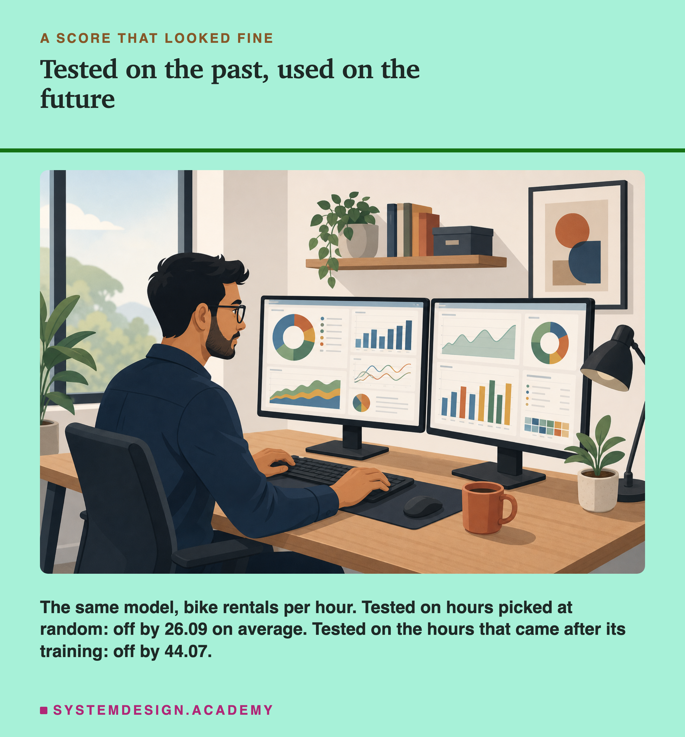
This lesson does the same thing to a computer program that guesses how many bikes a city rents in an hour. I tested it the usual way, on hours picked at random, and it looked good. Then I tested it on the hours that came after everything it had learned from, which is the only way it would ever be used. It missed by 1.69 times as much. The rest of the lesson measures where that extra error lives, and what to do so that your own tests tell you the second number before your users do.

The lesson before this one, the production gap, made one claim that this whole chapter now tests with real data: a program that learns from examples can look fine in testing and still go wrong once it is used, and nothing raises an alarm when it does. That lesson named four ways a shipped model breaks. This chapter measures failures like those, one at a time, on one public dataset, so that each lesson can be compared with the one before.

This chapter starts with a failure that lesson did not list: the test itself. The number that told you the program was good was computed in a way that the real world will never repeat. Nobody lied on purpose. The test was set up with a standard recipe, and the recipe quietly let the program see things that it will not see later. The score was honest about the test. The test was not honest about the job.

Here, the job is to guess bike rentals for hours that have not happened yet. The standard recipe mixed future hours into the learning and past hours into the test. That is not a mistake anyone would spot by reading the code. It is the standard recipe, and it is one line. The fix is also one line. What takes more work is knowing what the honest number is telling you, and that is most of this lesson.

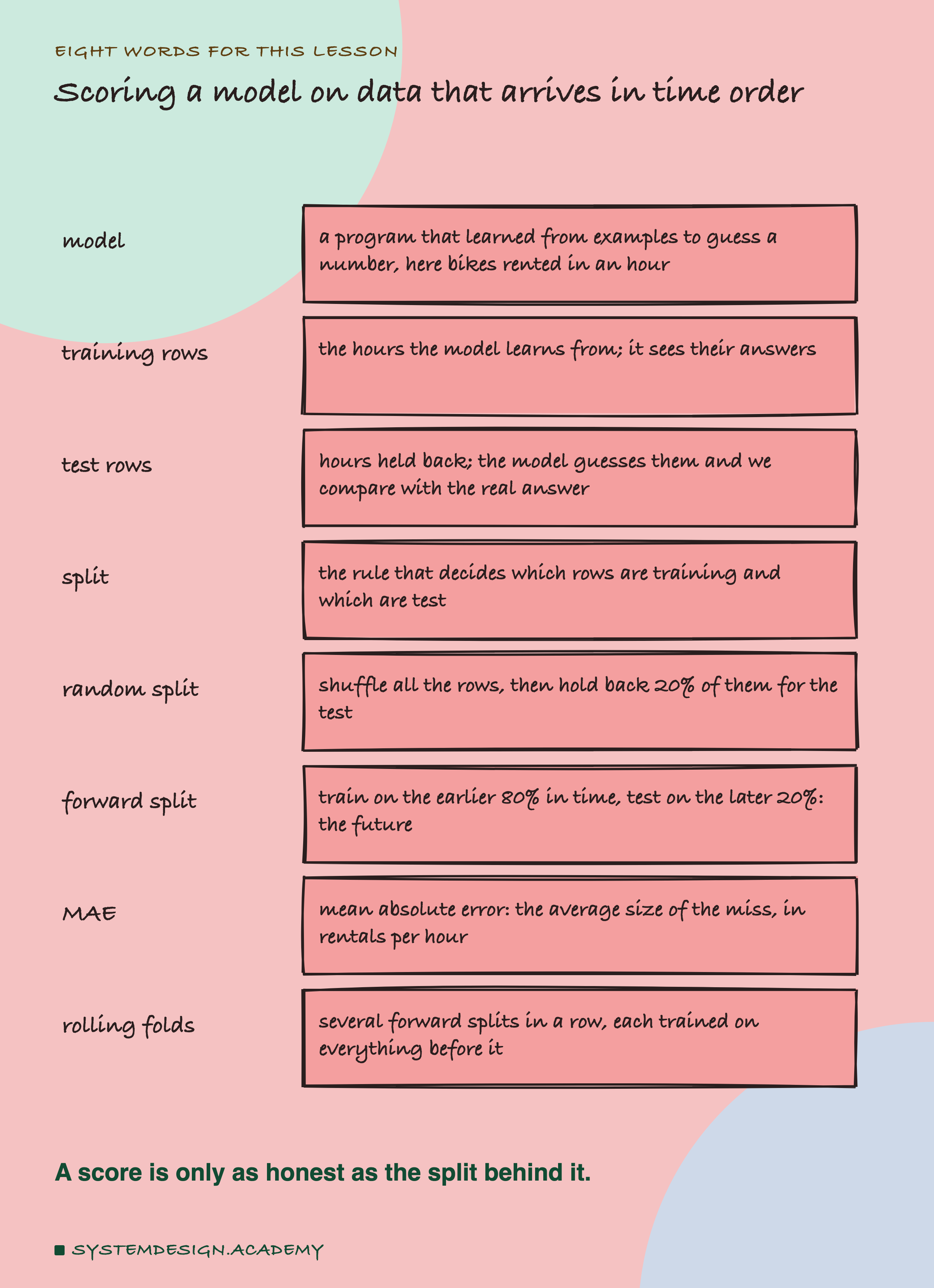
A model is a program that learned from examples to guess a number. It is not written by hand: it is shown many rows where the answer is known, and it finds its own way to guess the answer from the other columns. Here each row is one hour, and the number to guess is how many bikes were rented in it.

The rows it learns from are the training rows. The rows held back to check it are the test rows: the model guesses them without seeing their answers, and then we compare the guesses with the real answers. The split is the rule that decides which rows go where. A random split shuffles all the rows and holds back a fixed share, here 20%, for the test. A forward split keeps the rows in time order, trains on the earlier 80% and tests on the later 20%, which is the future from the model's point of view. Rolling folds are several forward splits in a row, each one trained on everything before its own test block.

The score in this lesson is the mean absolute error, shortened to MAE. For every test hour you take the difference between the guess and the real count, drop the minus sign, and average. Its unit is the same as the thing being guessed, rentals per hour, which is why I use it: "off by 26 bikes an hour" is something you can picture.

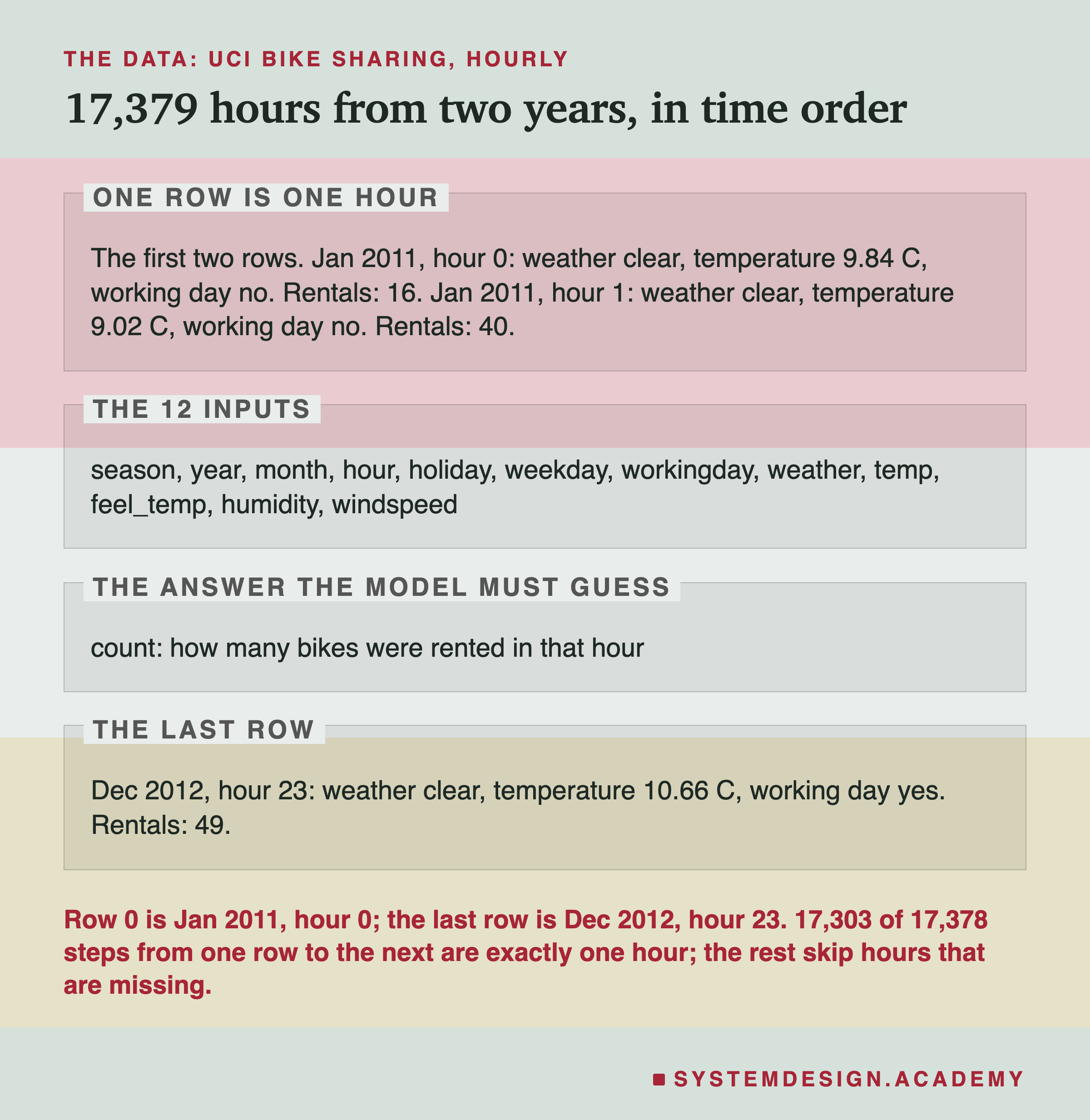
The data is the UCI Bike Sharing dataset, hourly version, from a bike rental scheme in Washington, D.C., in 2011 and 2012. I use the copy on OpenML, a free public website that stores datasets for machine learning (dataset 42712, version 2, listed with a public licence), because scikit-learn can download it in one line. It has 17,379 rows, one per hour, in time order. Each row has 12 inputs: the season, the year (0 for 2011, 1 for 2012), the month, the hour of the day, whether it was a holiday, the day of the week, whether it was a working day, a weather label (clear, misty, rain and so on), the temperature, the "feels like" temperature, the humidity and the wind speed. The answer to guess is count, the number of bikes rented in that hour.

Two things about this data matter for the whole lesson. First, the rows are in time order, and almost every row is exactly one hour after the one before it: 17,303 of the 17,378 steps from one row to the next are one hour, and the rest jump over hours that are missing from the file. So "the next row" nearly always means "the next hour". Second, nothing in the inputs says what happened on a particular day beyond the weather and the calendar. If there was a street festival, a train strike or a broken docking station, the model cannot know.

I chose this dataset for the chapter because it is public, small (it fits in under 1 MB on my disk), and it runs on any laptop with scikit-learn and no special hardware. Every later lesson in the chapter uses it too.

Everything in this lesson comes from one choice: which 20% of the hours to hold back.

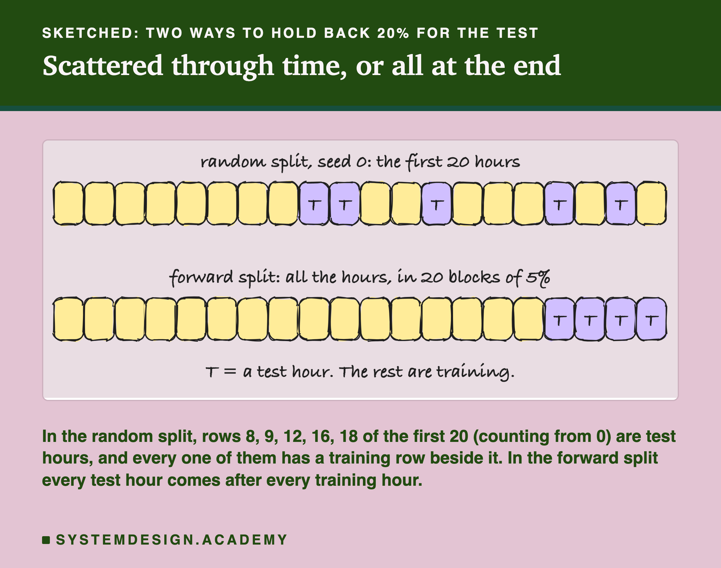
The random split is the standard recipe. scikit-learn's train_test_split shuffles the rows with a fixed seed (a starting number for the shuffle, so that the same seed always gives the same shuffle) and holds back 20%. The top strip above is the real result of seed 0 on the first 20 hours of the data: rows 8, 9, 12, 16 and 18 went to the test, and the hours around them went to training. The test hours are scattered through all two years, like the torn-out diary pages.

The forward split keeps time in order. The first 80% of the rows, 13,903 hours from January 2011 to August 2012, are training. The last 20%, 3,476 hours from August 2012 (starting at hour 12 of one August day) to the end of December 2012, are the test. No test hour comes before any training hour. This is the shape of real use: a model is trained on what has happened and then asked about what has not.

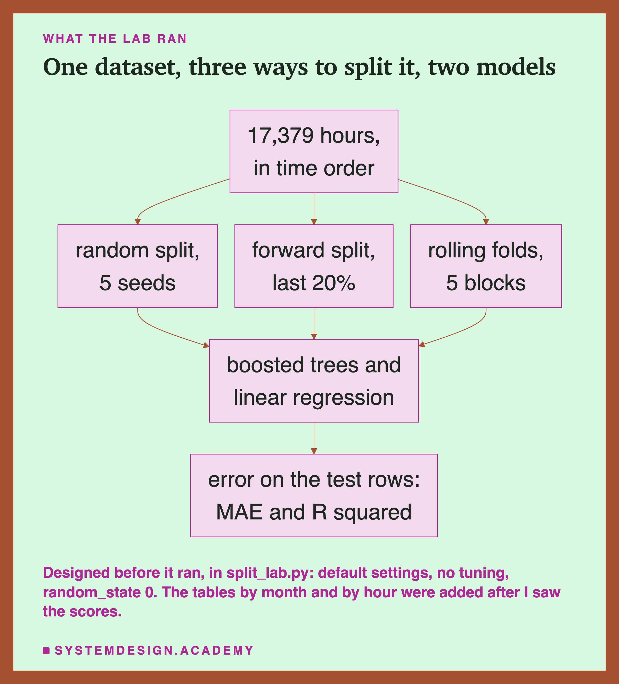
The lab ran both splits, plus a third kind, rolling folds, which the later slides explain. It ran each on two models, so that the result is not about one model's quirks.

I wrote the design down at the top of the lab file, split_lab.py, before I ran it: the question, the data, the two models, the three kinds of split, the two scores, and that the gap would be reported as the forward error divided by the random error. The dated record is the chapter plan, CHAPTER-PLAN.md (2026-09-29, "SPLIT LAB (batch 1) designed before running").

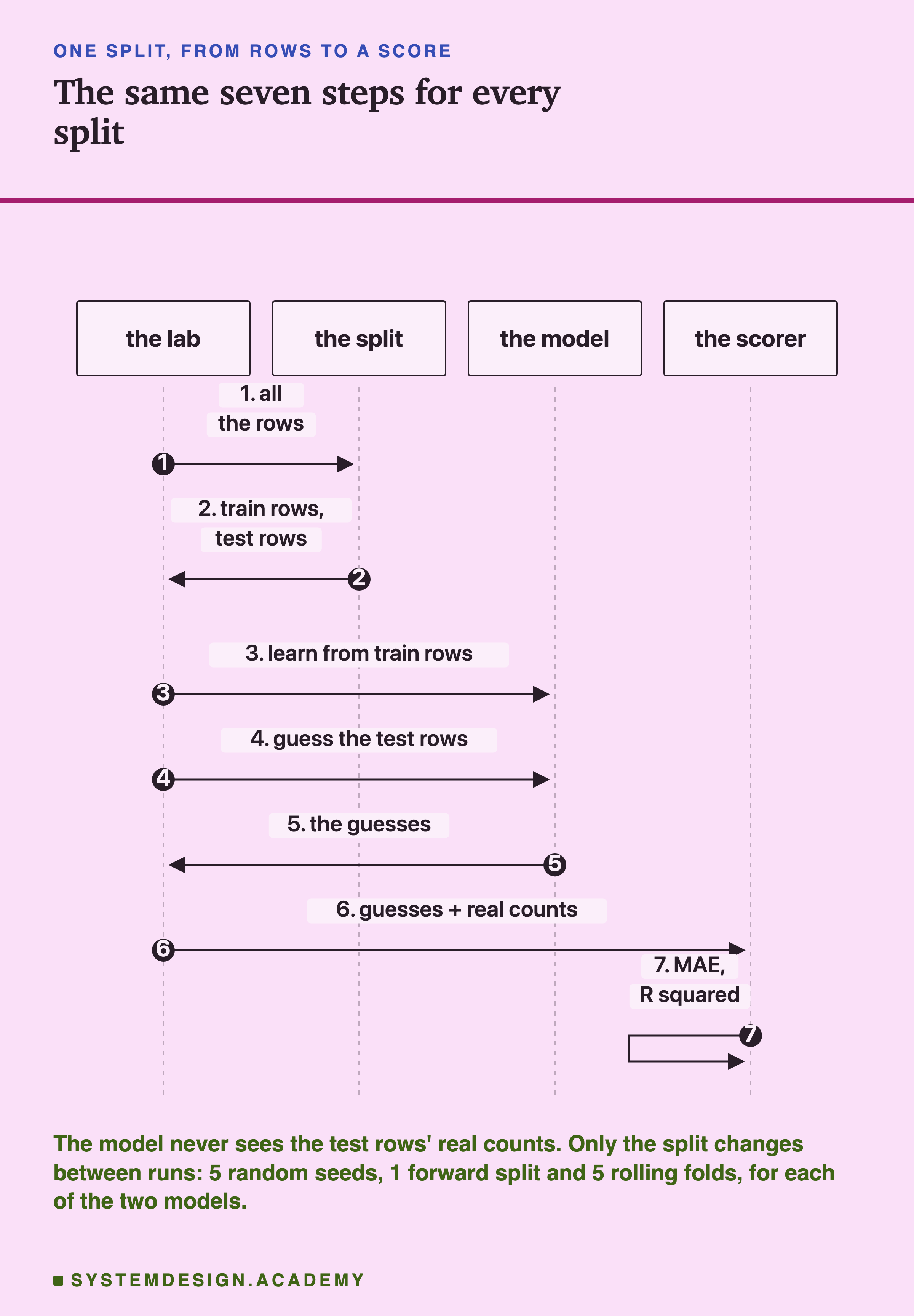
The two models. The first is scikit-learn's HistGradientBoostingRegressor, which I call boosted trees. A decision tree guesses a number by asking a chain of yes-or-no questions about the inputs ("is the hour after 7? is it a working day?") and giving the average answer of the training rows that end up in the same place. Boosting builds many small trees one after another (up to 100 with scikit-learn's default settings), each one correcting the errors the earlier ones left. It is a strong, common choice for tables of numbers. The second model is linear regression, which guesses by adding up a fixed weight for each input. It is much weaker here, and it is in the lab as a check: if both a strong and a weak model show the same pattern, the pattern is less likely to be about one model.

No tuning. A model's settings are choices made before it learns, such as how many trees to build or how deep each one may grow. Tuning means trying many settings and keeping the ones that score best. Both models ran with scikit-learn's default settings and random_state=0, a fixed seed for the model's own random choices. I did not try other settings. Tuning could change both scores; it would not change which split the real world repeats.

Before the results, here is what the main score means, on three real test hours.

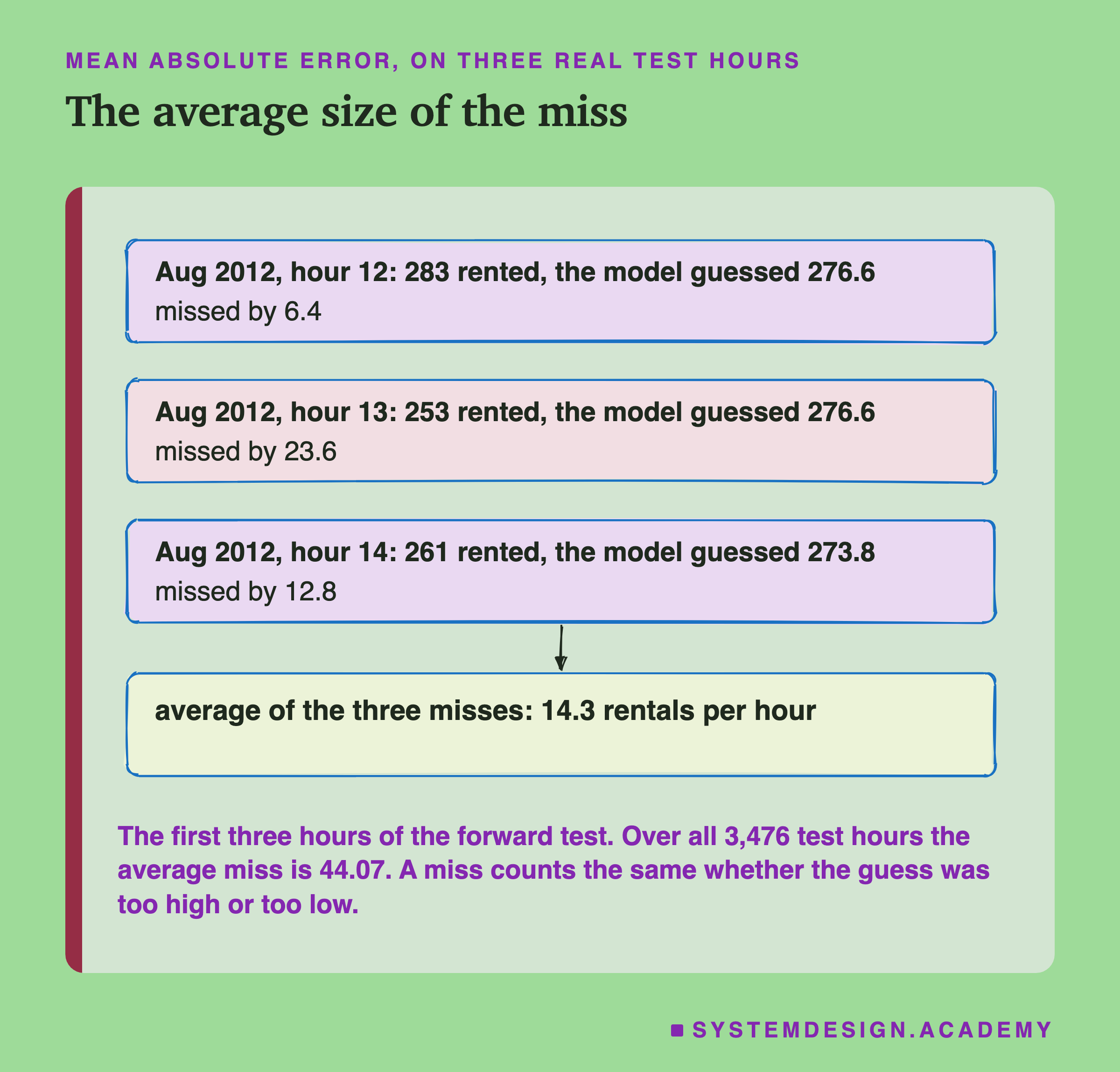
These are the first three hours of the forward test, with the boosted trees' real guesses. At hour 12, 283 bikes were rented and the model guessed 276.6, a miss of 6.4. At hour 13 the real count was 253 against the same guess of 276.6, a miss of 23.6. At hour 14, 261 against 273.8, a miss of 12.8. The average of the three misses is 14.3. Do that over all 3,476 test hours and you get the forward MAE, 44.07. A guess that is 20 too high and a guess that is 20 too low both count as a miss of 20. That is what "absolute" means: the minus sign is dropped.

The lab also stored a second score, R squared. It compares the model with the laziest possible guess, always saying the average count of the test hours. An R squared of 1 means every hour was guessed exactly; 0 means the model did no better than the lazy guess.

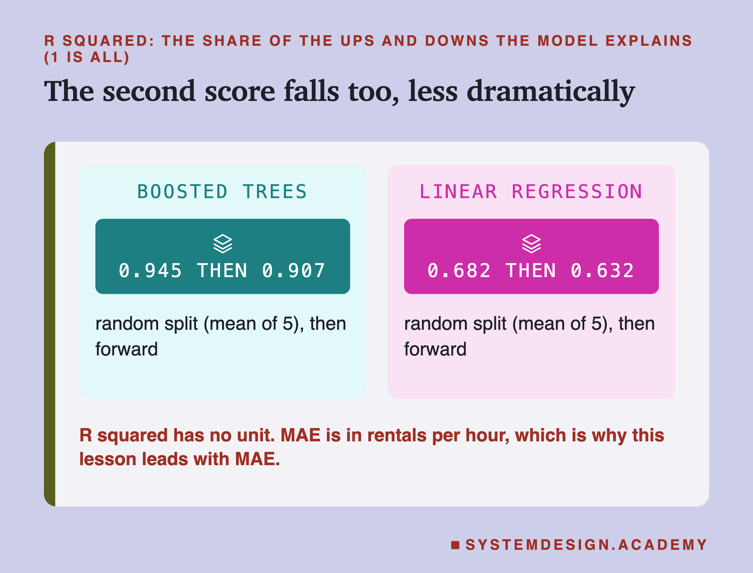
For the boosted trees, R squared was 0.945 on the random splits (the mean of the five) and 0.907 on the forward split. For the linear model, 0.682 and 0.632. Both scores fall on the future, for both models. I lead with MAE because it keeps the unit: a drop from 0.945 to 0.907 sounds small, but the same runs, measured in bikes, are a miss that grew from about 26 an hour to about 44.

Here is the headline, straight from the lab's stored file, results/split.json.

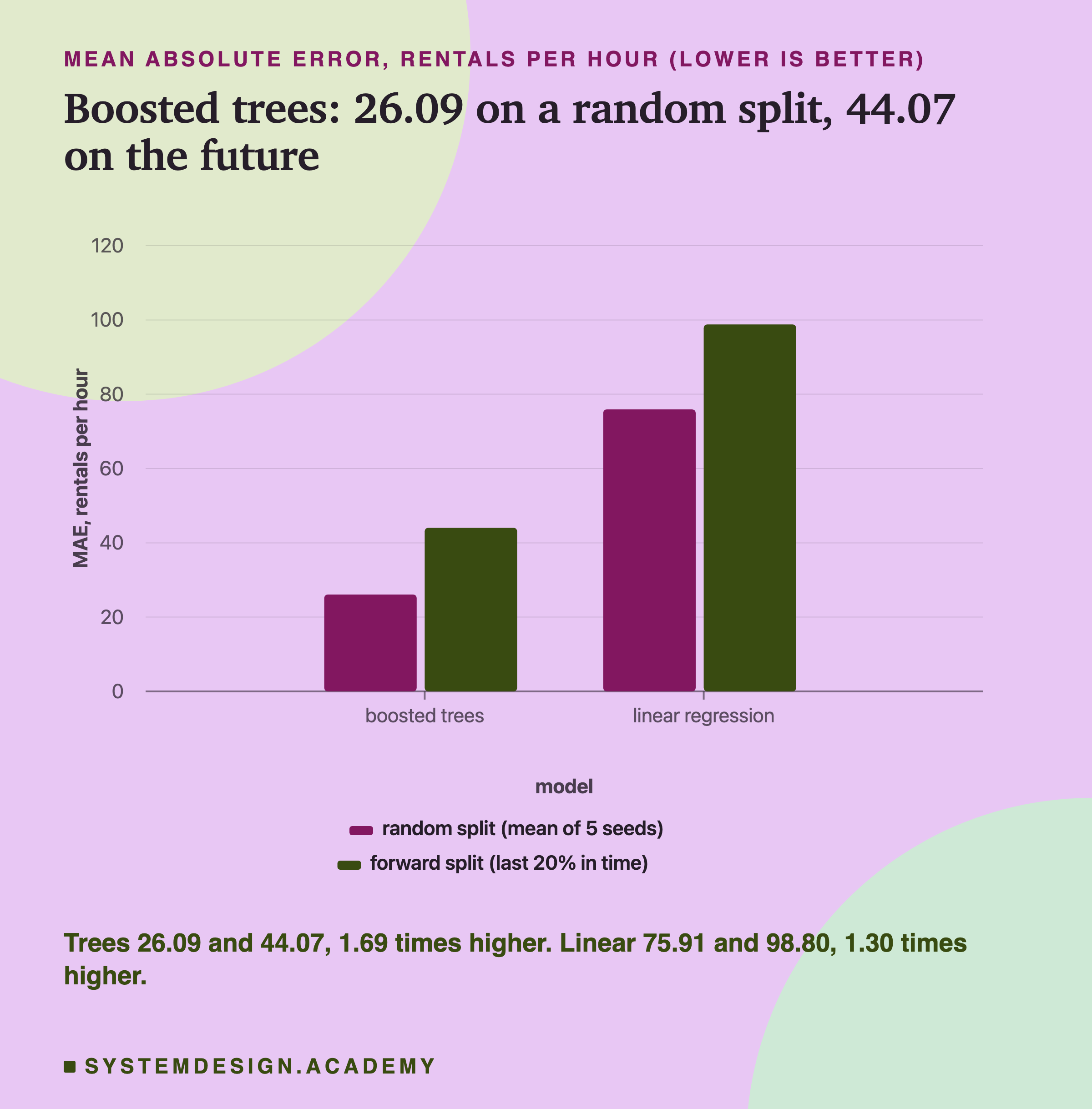
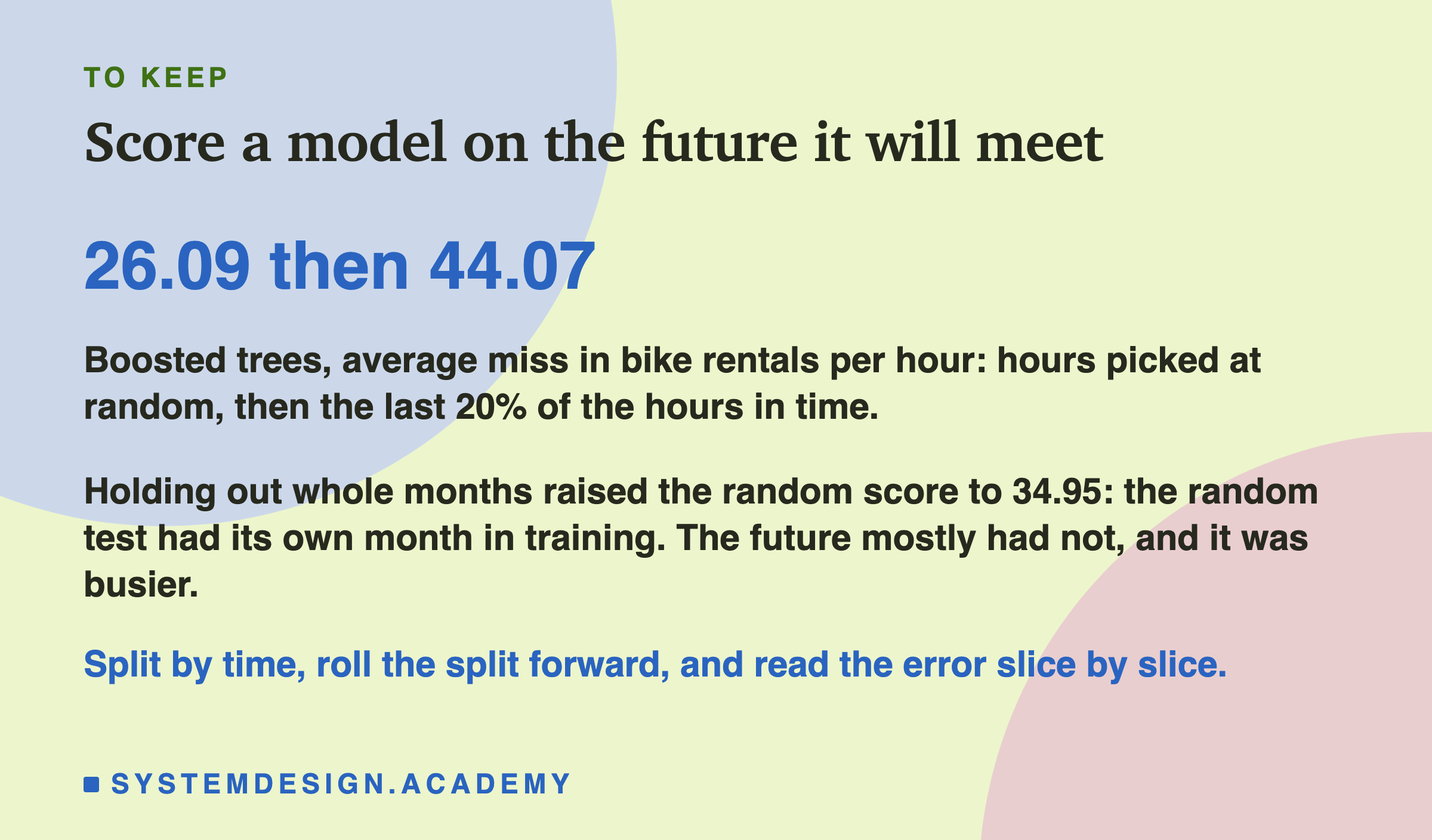
On the random splits, the boosted trees missed by 26.09 rentals an hour on average, the mean over five seeds. On the forward split, they missed by 44.07. That is 1.69 times as much. The linear model went from 75.91 to 98.80, 1.30 times as much. Same data, same model, same settings; only the choice of test hours changed.

If you had built this model with the standard recipe, you would have written "MAE about 26" in your report. The forward test, which is the shape of real use, showed 44. Nothing in the code would be wrong. The report would just describe a job the model was never going to do.

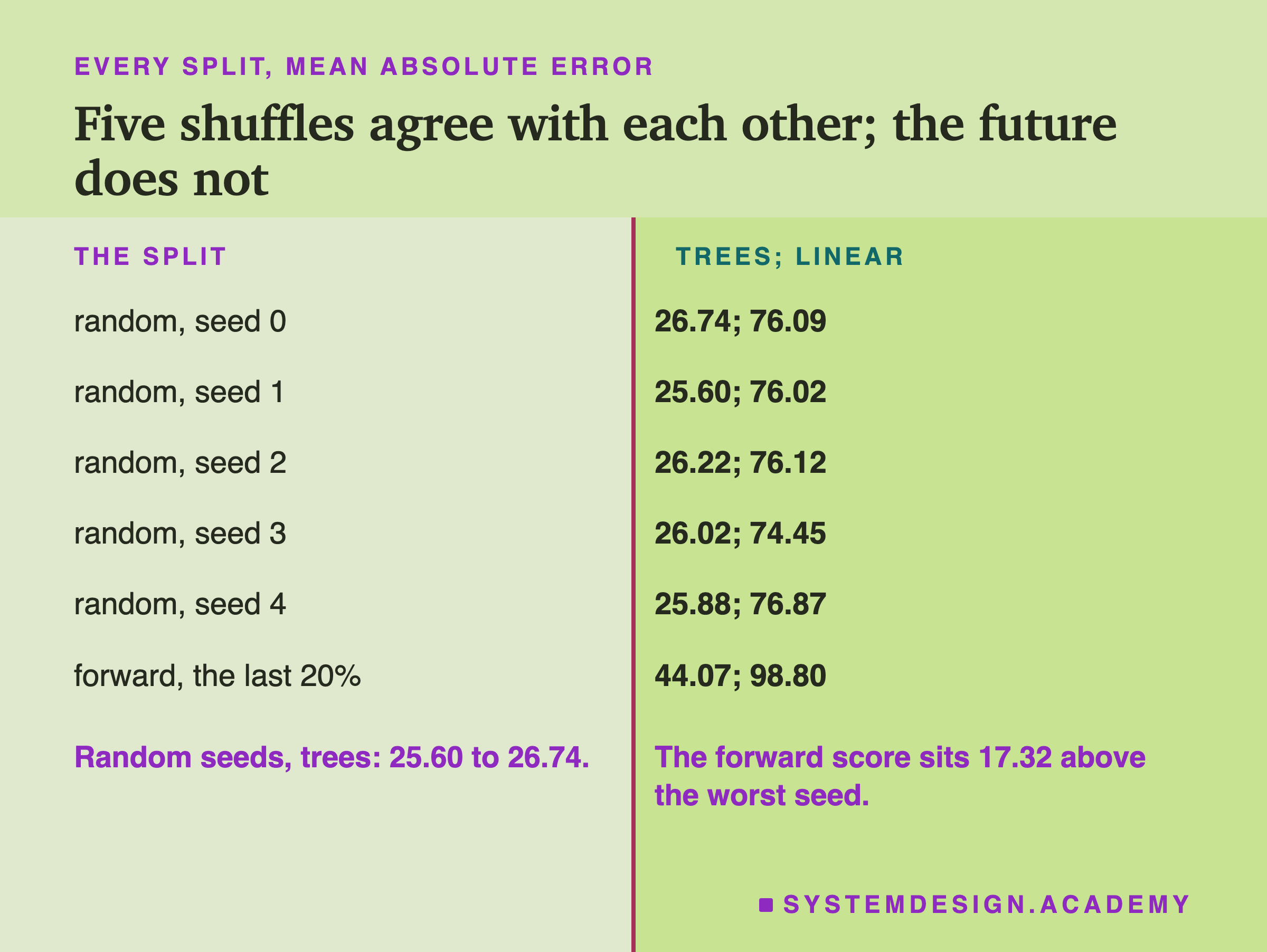
Why five random seeds? Because a single random split is itself a roll of the dice, and I wanted to know how much the random score moves on its own. For the trees it moved between 25.60 and 26.74, about one bike an hour. The forward score, 44.07, is 17.32 above the worst of the five. So the gap is not the random split being unlucky once: five different shuffles all told the same flattering story.

There is one forward split, though, and one future. The rolling folds, later in the lesson, show how much a forward score moves from one stretch of time to another. It moves a lot more than the random seeds do.

Before I asked why the model did worse on the future, I checked something duller: were the future hours simply bigger numbers? A miss of 44 on hours that average 250 rentals is not the same as a miss of 44 on hours that average 150.

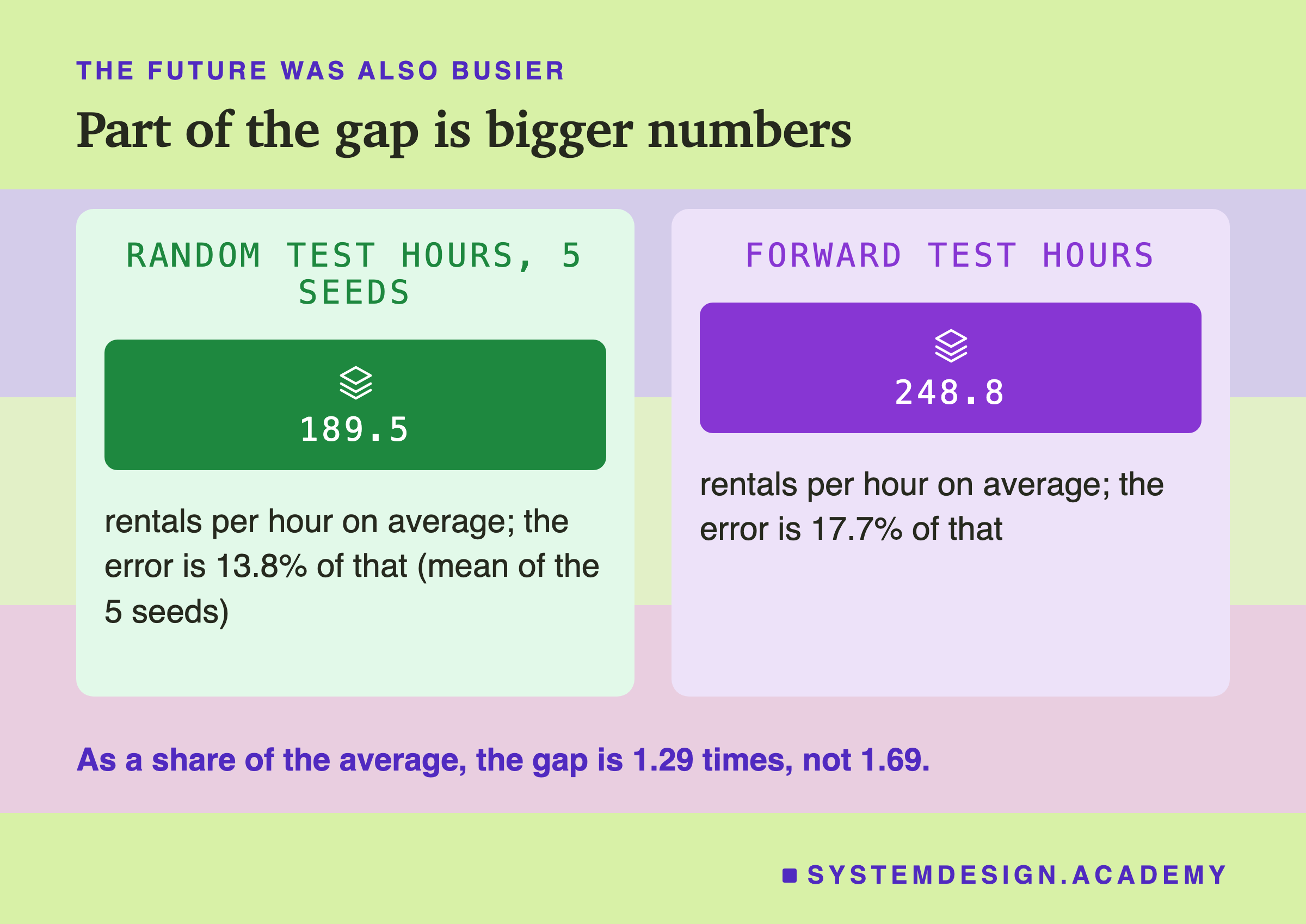
They were. The random test hours averaged about 190 rentals an hour (from 186.1 to 191.5 over the five seeds, close to the whole dataset's 189.5). The forward test hours averaged 248.8. The last months of the data were busier than the data as a whole, because, as a later slide shows, the second year was much busier than the first.

So I divided each error by the average count of its own test hours. For the random splits the error was between 13.4% and 14.1% of the average, 13.8% as the mean of the five. For the forward split it was 17.7%. Measured that way the gap is 1.29 times, not 1.69. I added this measure after I saw the results, and I think it belongs in the lesson because it changes how big the problem looks.

Both numbers are true, and they answer different questions. If you need to know how many bikes you will be wrong by, which is what a person planning trucks and staff needs, the answer is the MAE, 44.07, and that is 1.69 times what the random split promised. If you want to know whether the model got worse at its job apart from the job getting bigger, the share says: yes, still worse, by about 29% (17.7% against 13.8%). Either way the random split told you less than the truth.

The lab stored the trees' guess for every forward test hour, so the error can be read by slice of time. I read those guesses before writing anything about why the error was higher. Here is the average real count and the average guess for each month of the test.

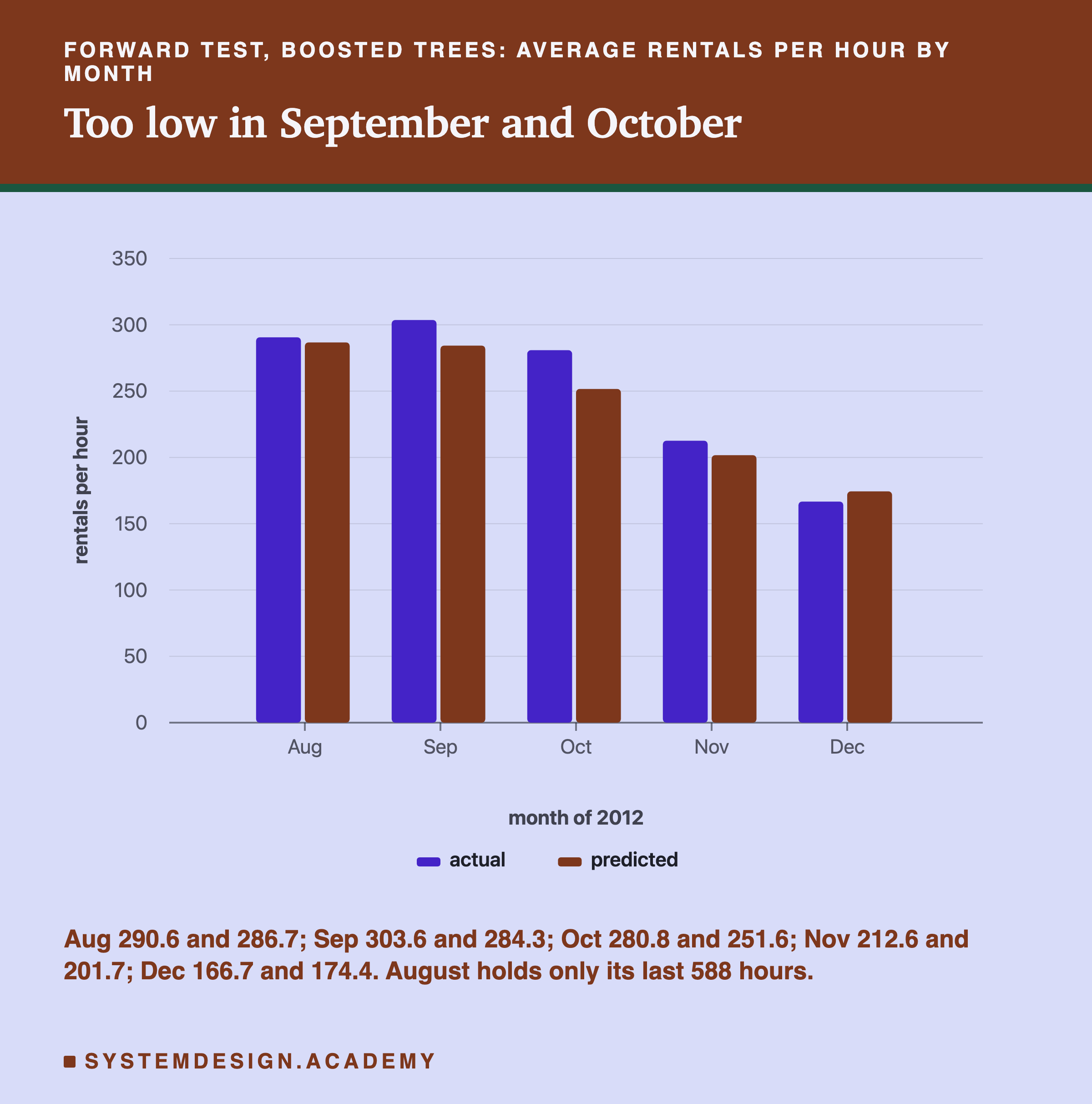
In the last part of August, the first stretch of the test, the model's average guess was close: 286.7 against a real 290.6. In September it guessed 284.3 against 303.6, and in October 251.6 against 280.8. On average, it guessed too low in those two months by about 19 and 29 bikes an hour. In November it was still a little low, and in December a little high.

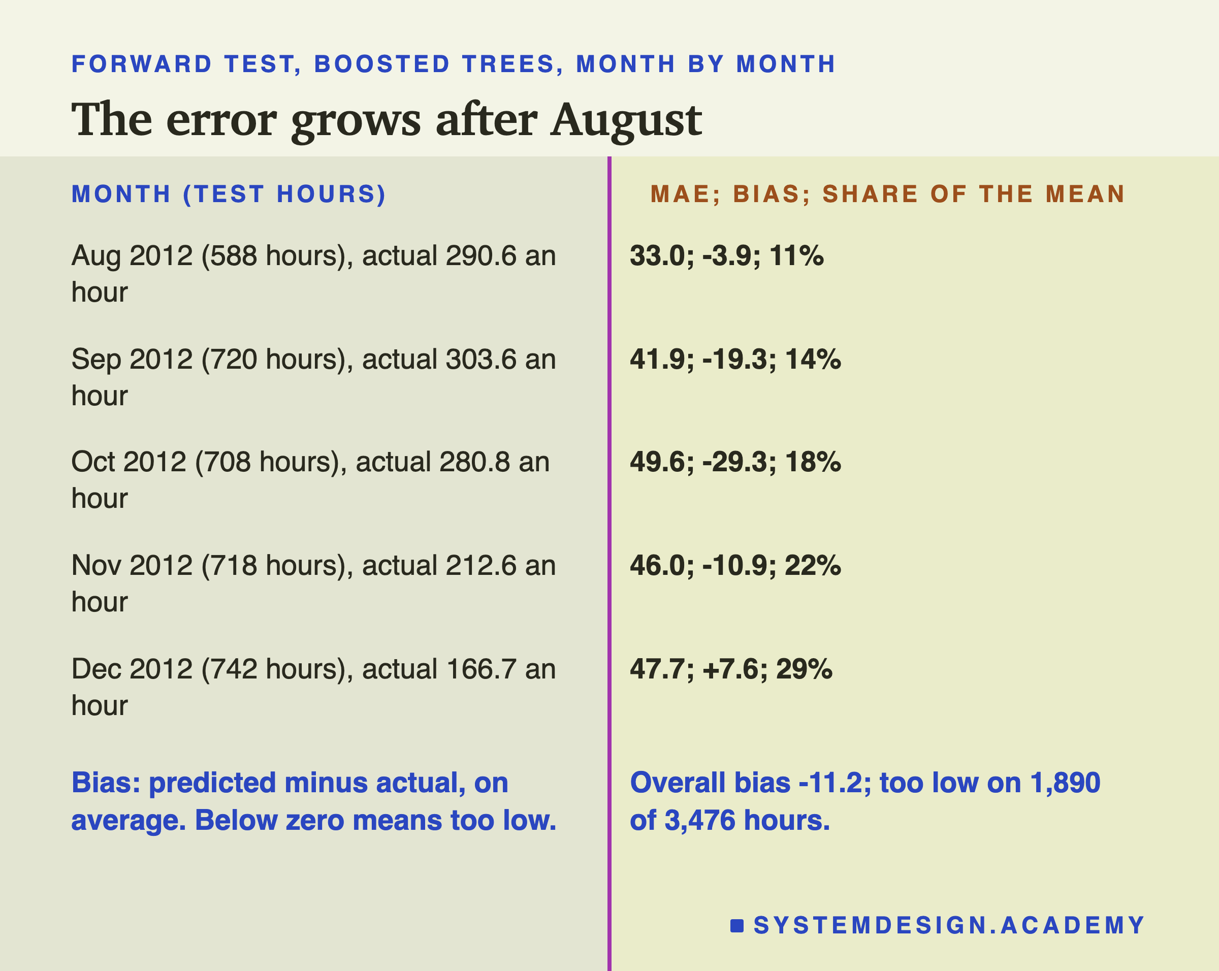
The bias column is the average of the guess minus the real count, keeping the sign, so it shows direction: below zero means the model guessed too low on average. The MAE was 33.0 in the part of August closest to the training data, then 41.9, 49.6, 46.0 and 47.7. Over the whole test the bias was -11.2: the model was too low on 1,890 of the 3,476 hours.

The last column changes the picture again. December's MAE, 47.7, is close to November's 46.0, but December was quieter, 166.7 rentals an hour against 212.6, so the error is 29% of the average, the largest share of any month. The further the test month is from the training data, the bigger the error is as a share of what happened, and part of that rise is simply the months getting quieter while the misses stay about the same size. That is measured. Why the misses stay that size is the next question, and this slide cannot answer it alone.

One more thing from the same table: the linear model's error by month (in the lab report) was 103.3, 122.3, 110.6, 81.8 and 77.6. It did worst in September, when the counts were highest.

The same forward guesses, grouped by the hour of the day instead of the month.

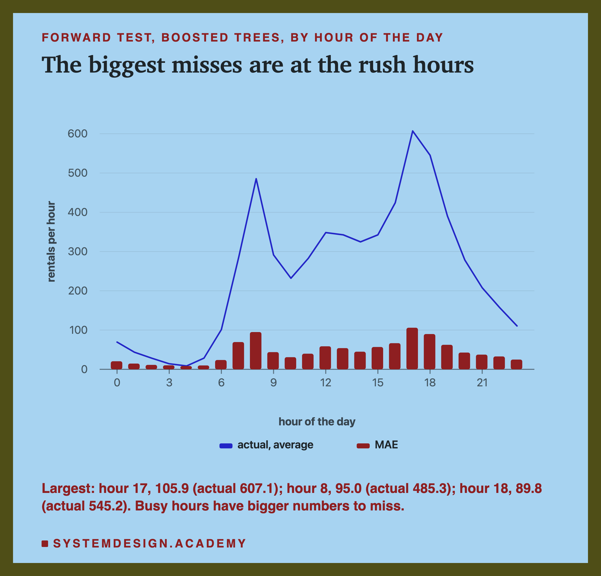
The biggest misses are at the commuting peaks: 105.9 bikes an hour at hour 17, 95.0 at hour 8 and 89.8 at hour 18. At hour 4, when about 9 bikes an hour were rented, the MAE was 8.4. In bikes, the peaks miss most because they have the most bikes. As a share of each hour's own average the picture turns over: the miss at hour 17 was about 17% of its average count, and at hour 4 about 97%. In proportion, the quiet night hours are the hardest to guess.

Two other groupings from the report are worth knowing. On working days (2,349 test hours) the MAE was 42.0 and the bias -15.6: the model was too low on working days. On days off (1,127 hours) the MAE was 48.3 but the bias only -2.1: bigger misses, but not mostly in one direction. By weather, the 238 test hours labelled rain had the biggest MAE, 73.3, against 40.6 for clear hours and 44.7 for misty ones.

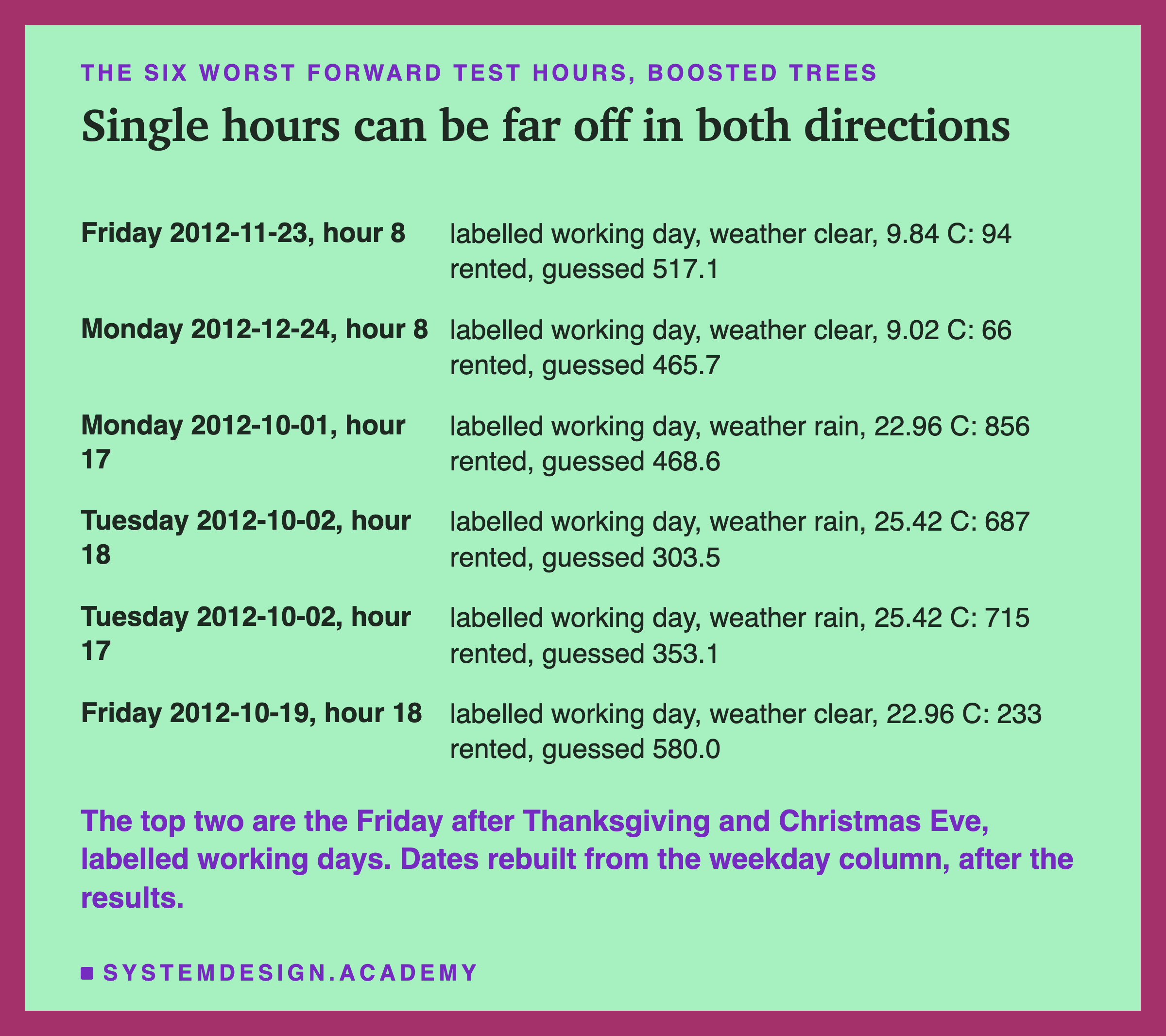
I read the worst single hours too, because an average can hide a few enormous misses. The file has no date column, so after I saw the results I rebuilt the dates: the day number rises by one each time the day of the week changes. That gives 731 days ending on 31 December 2012, and every rebuilt date agrees with the row's month, year and day of the week. The two worst hours are 8 in the morning on Friday 23 November 2012, the day after Thanksgiving in the United States, and on Monday 24 December 2012, Christmas Eve. The data labels both as working days and not holidays, although many people were off work on those days. 94 and 66 bikes were rented, and the model guessed 517.1 and 465.7: it did what the labels told it. I found this after the results, and I have not checked the scheme's own records for those two days. The third worst went the other way: an October rush hour labelled rain, 856 rented against a guess of 468.6. For that one the inputs give no reason; one possible reason, only a guess, is that the weather label describes only part of the hour. No split can fix that kind of miss. What a forward split does is stop you from being surprised that it exists.

To see why the model guessed low in September and October, I compared the two years, measured rather than assumed.

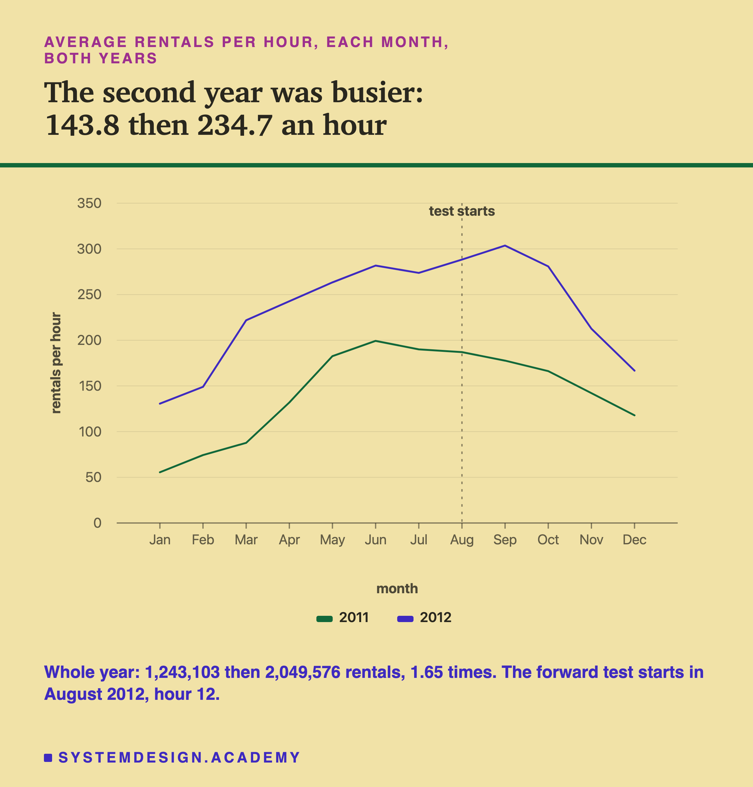
Rentals grew a lot. The whole of 2011 had 1,243,103 rentals and the whole of 2012 had 2,049,576, 1.65 times as many. Per hour, that is 143.8 on average in 2011 and 234.7 in 2012. Every single month of 2012 was busier than the same month of 2011, from 1.41 times (June and December) to 2.53 times (March). The growth was a little larger on working days (144.9 to 241.2 an hour) than on days off (141.5 to 220.7).

The shape of the year changed too. In 2011, the busiest months were June and July, and September was already quieter than August. In 2012, September was the busiest month of all, busier than August.

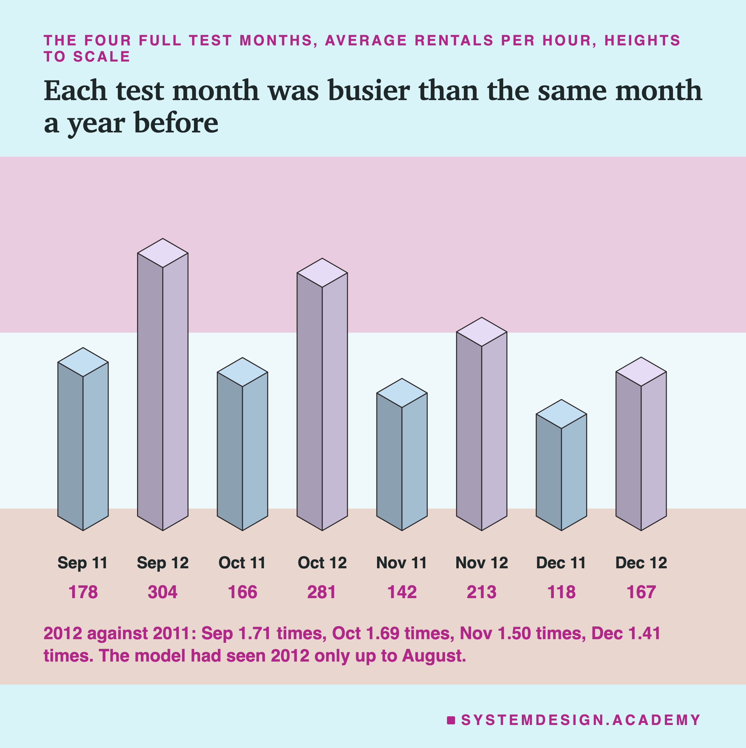
Now put that next to the forward split. The model was trained on all of 2011 and on 2012 up to August. It had seen how busy 2012 was in its first eight months, and it had seen how the autumn went in 2011, when rentals fell from August onwards. It had never seen an autumn of 2012. Here is one possible reason for the low guesses in September and October, and it is a guess, not a measurement: the model combined the 2012 level it had seen with the 2011 autumn shape it had seen, and so expected September and October 2012 to fall away from August the way 2011 did.

They did not. The data cannot prove that this is how the trees reasoned; what it does show is that the months where the model was most too low are the months where 2012 differed most from the 2011 pattern.

The months explain why the future was hard. They do not yet explain why the random split was easy. First I counted, for each test hour, what the model had in its training data around it. I added these counts after I saw the results.

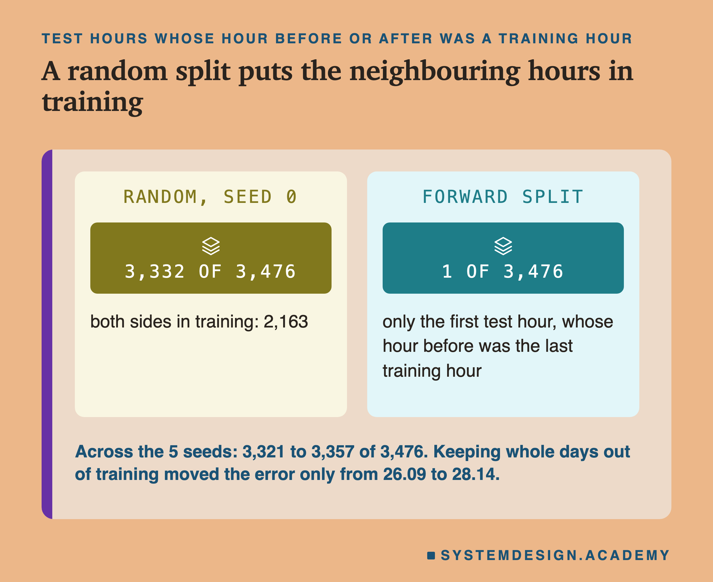
With seed 0, 3,332 of the 3,476 random test hours had the hour just before or just after them in the training data, and 2,163 had both. Across the five seeds it was between 3,321 and 3,357. With the forward split, exactly 1 test hour had a training neighbour: the very first one, whose hour before was the last hour of training.

A count is not a cause. The model never sees any test hour's count, and it has no input for the day of the month, so it cannot look up "the hour before" at all. What it can do is learn from training hours that share its inputs: the same year, the same month, the same hour of the day, similar weather. Whether the neighbouring hours matter is a question for a test, and the next figure is that test.

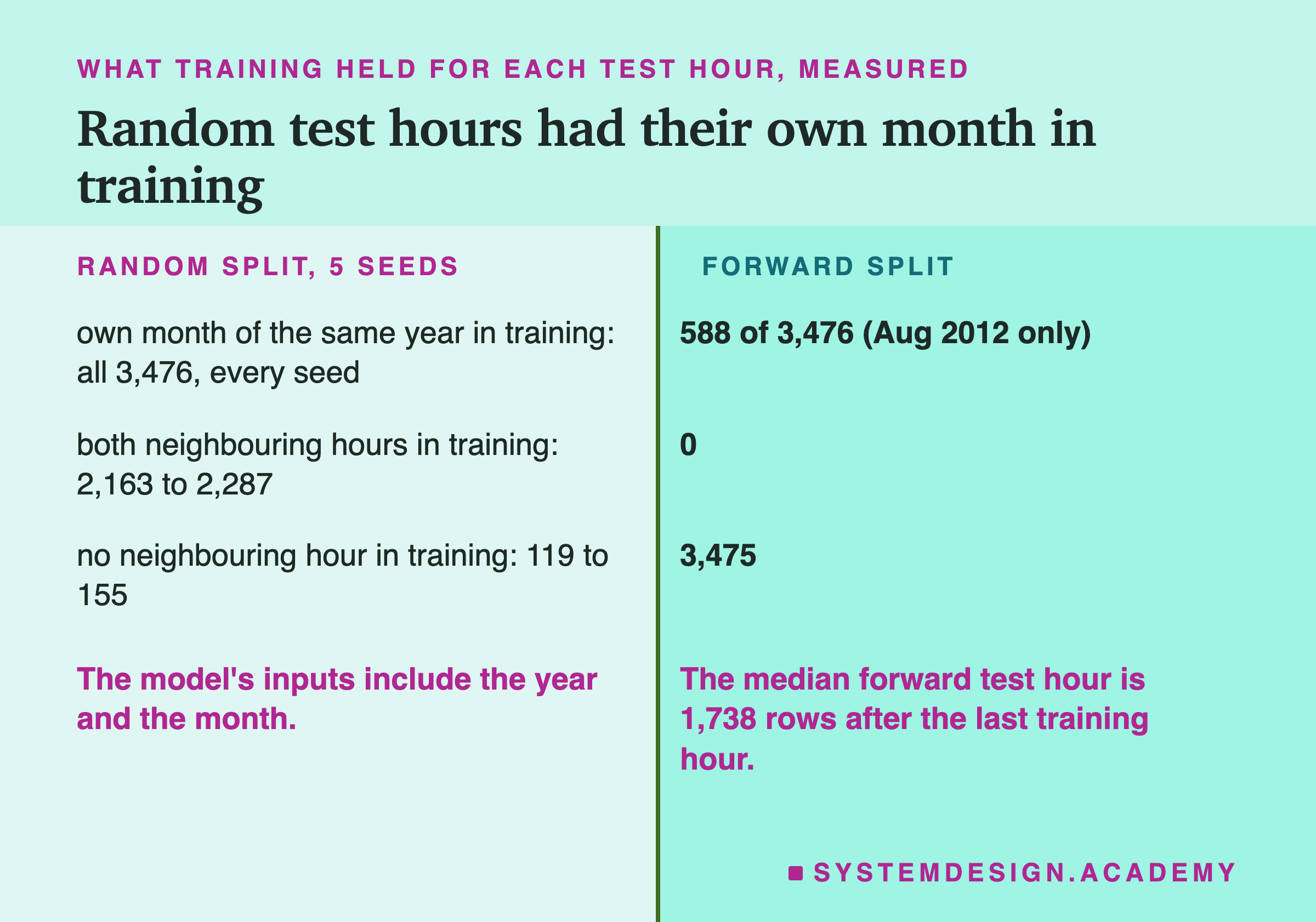
The neighbouring hour is the narrow case. The wider one is the month. The model's inputs include the year and the month, so it can learn how busy "October 2012" was, but only if some hours of October 2012 are in its training data. With every random seed, all 3,476 test hours had other hours of their own month of the same year in training. With the forward split, only 588 did: the hours from the last part of August 2012. For September to December 2012, the model had no hour at all from that month of that year. The median forward test hour (the middle one, if you line them all up by distance) is 1,738 rows, about ten weeks, after the last hour the model learned from.

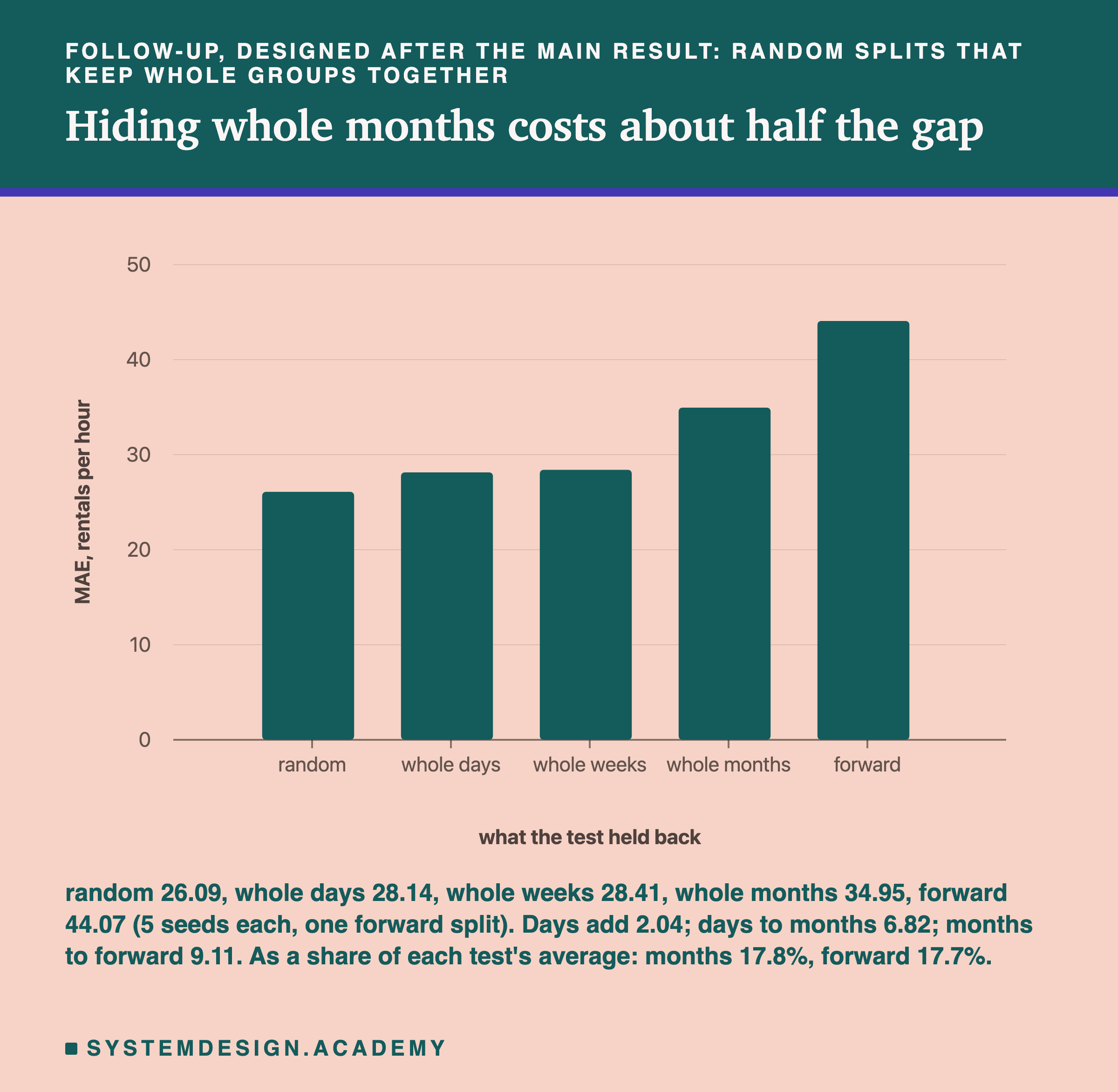
A review of this lesson pointed out that these counts show what training held, not what the model used. So I added a follow-up to the lab, designed after the main results and prompted by that review. Its design is the description of the lab's mode, and its results are in . It runs random 80/20 splits again, but keeps whole groups on one side, so that no test hour has any member of its group in training. The groups are whole days (the file has no date column, so the day is rebuilt the way the worst-hours slide describes, which gives 731 days), whole weeks, and whole calendar months. Five seeds each, the same boosted trees, the same inputs.

One forward split gives one number about one future. Rolling folds give several. The lab used scikit-learn's TimeSeriesSplit with 5 folds: it cuts the rows into six blocks of about the same size, in time order, then for each fold trains on every block before the test block and tests on the next one. The first fold trains on the first block only; the fifth trains on five blocks.

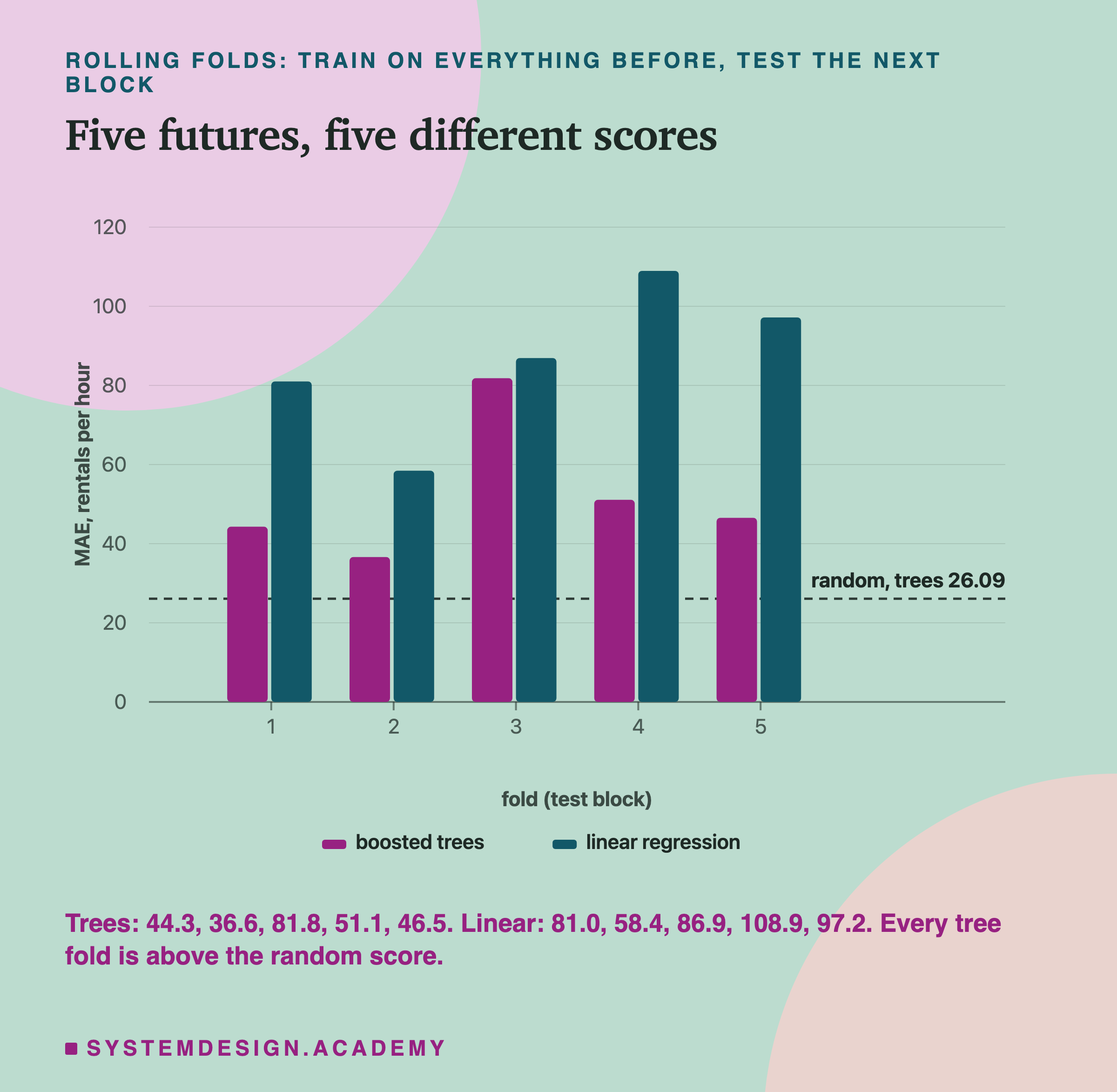
For the boosted trees the five folds scored 44.3, 36.6, 81.8, 51.1 and 46.5 rentals an hour. Every one is above the random-split score of 26.09. And they are far apart from each other: the worst is more than twice the best. Five random seeds moved by about one bike an hour; five stretches of the future moved by 45.

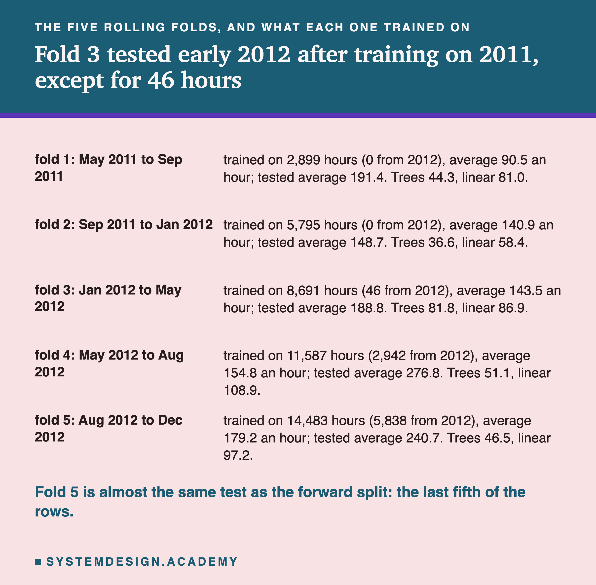
The table shows what each fold had to work with. Fold 3 is the striking one. It tested January to May 2012 after training on 2011 and only the first 46 hours of 2012. The model had almost no example of the busier second year, and the test hours averaged 188.8 against a training average of 143.5. Its error, 81.8, was the worst of the five. Fold 2, which tested September 2011 to January 2012 after training on January to September 2011, did best at 36.6; its test hours were close to its training average (148.7 against 140.9). Fold 5 tests almost the same hours as the forward split and scored 46.5, near the forward split's 44.07; its cut point is 580 rows later, so it trains on a little more and tests on a little less.

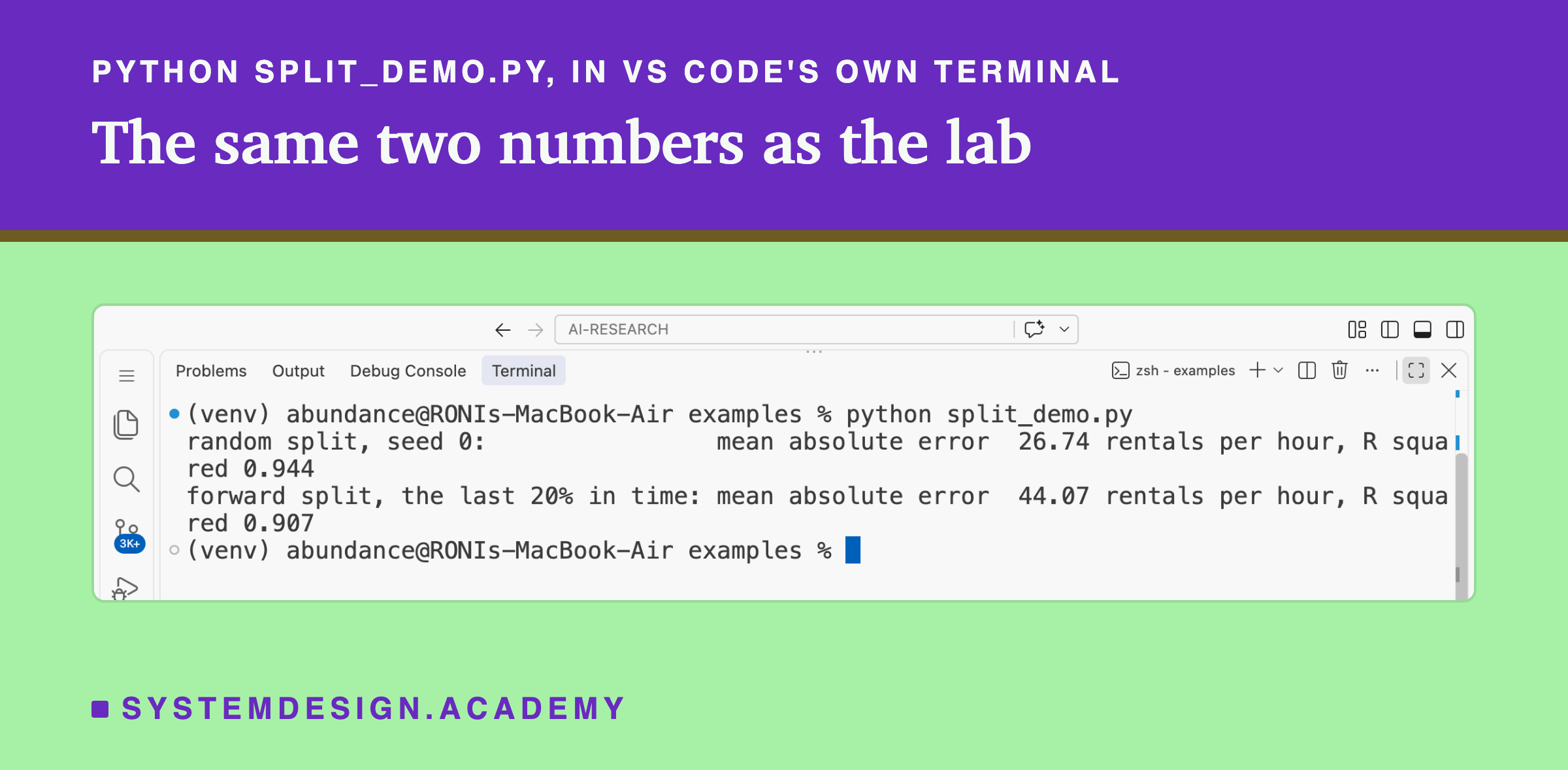
This script is the lab made small. It downloads the same data, trains the boosted trees once on a random split (seed 0) and once on the forward split, and prints both errors. It does not need a GPU.

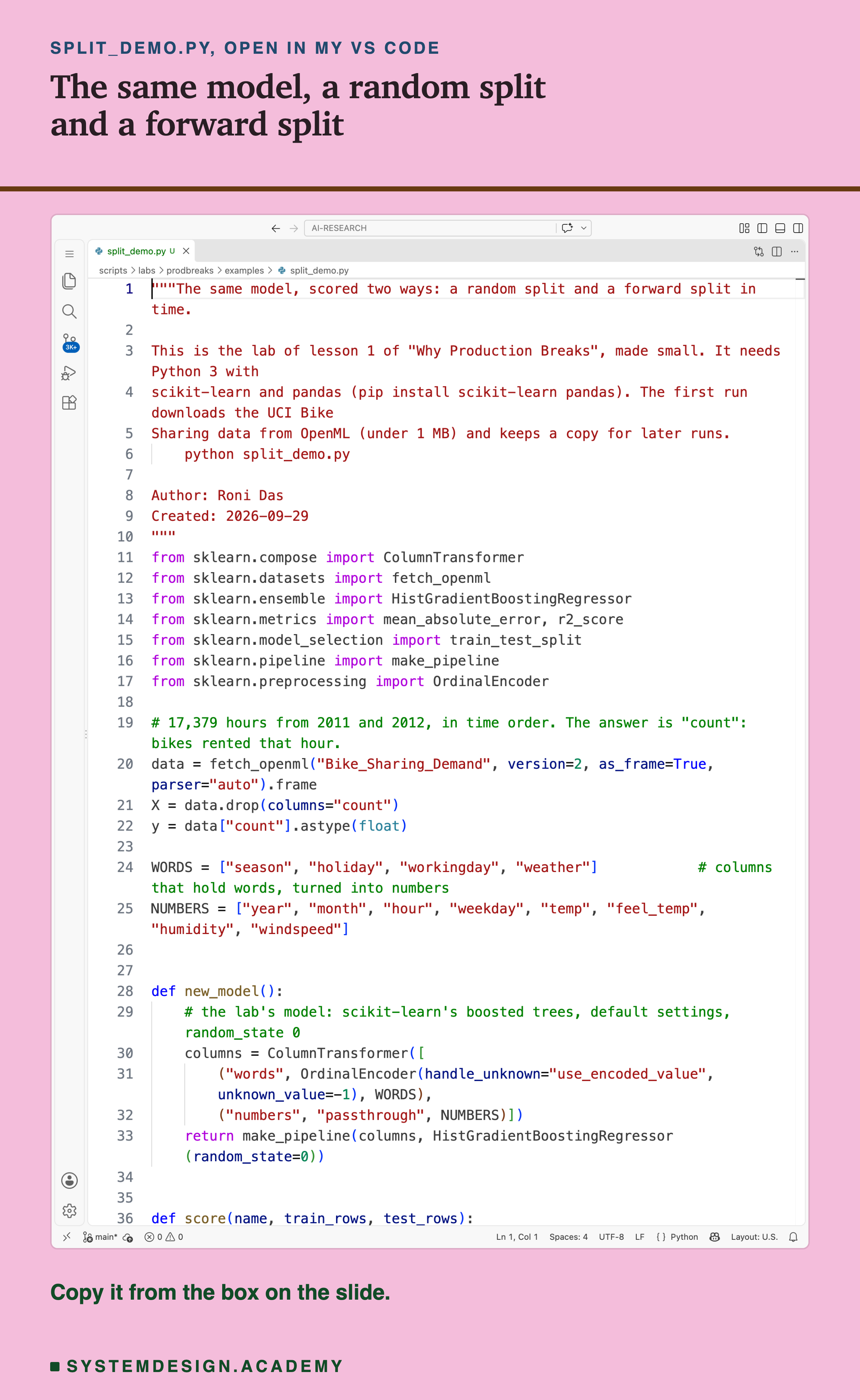
Before you run this lab. You need Python 3 and two libraries: pip install scikit-learn pandas. scikit-learn holds the models, the splits and the download; pandas holds the table. The first run downloads the Bike Sharing data from OpenML, so it needs an internet connection once; scikit-learn keeps a copy in a folder in your home directory (scikit_learn_data) for later runs. I ran it with scikit-learn 1.9.1 on a Mac. scikit-learn runs the same way on Windows and Linux, but I have not checked the numbers there, and another version of scikit-learn may give slightly different decimals.

"""The same model, scored two ways: a random split and a forward split in time.

This is the lab of lesson 1 of "Why Production Breaks", made small. It needs Python 3 with
scikit-learn and pandas (pip install scikit-learn pandas). The first run downloads the UCI Bike
Sharing data from OpenML (under 1 MB) and keeps a copy for later runs.
    python split_demo.py

Author: Roni Das
Created: 2026-09-29
"""
from sklearn.compose import ColumnTransformer
from sklearn.datasets import fetch_openml
from sklearn.ensemble import HistGradientBoostingRegressor
from sklearn.metrics import mean_absolute_error, r2_score
from sklearn.model_selection import train_test_split
from sklearn.pipeline import make_pipeline
from sklearn.preprocessing import OrdinalEncoder

# 17,379 hours from 2011 and 2012, in time order. The answer is "count": bikes rented that hour.
data = fetch_openml("Bike_Sharing_Demand", version=2, as_frame=True, parser="auto").frame
X = data.drop(columns="count")
y = data["count"].astype(float)

WORDS = ["season", "holiday", "workingday", "weather"]            # columns that hold words, turned into numbers
NUMBERS = ["year", "month", "hour", "weekday", "temp", "feel_temp", "humidity", "windspeed"]


def new_model():
    # the lab's model: scikit-learn's boosted trees, default settings, random_state 0
    columns = ColumnTransformer([
        ("words", OrdinalEncoder(handle_unknown="use_encoded_value", unknown_value=-1), WORDS),
        ("numbers", "passthrough", NUMBERS)])
    return make_pipeline(columns, HistGradientBoostingRegressor(random_state=0))


def score(name, train_rows, test_rows):
    model = new_model().fit(X.iloc[train_rows], y.iloc[train_rows])
    guess = model.predict(X.iloc[test_rows])
    mae = mean_absolute_error(y.iloc[test_rows], guess)
    r2 = r2_score(y.iloc[test_rows], guess)
    print(f"{name:<36} mean absolute error {mae:6.2f} rentals per hour, R squared {r2:.3f}")


rows = list(range(len(y)))
cut = int(0.8 * len(rows))

# Random split: shuffle the hours, train on 80%, test on the other 20%.
train, test = train_test_split(rows, test_size=0.2, random_state=0, shuffle=True)
score("random split, seed 0:", train, test)

# Forward split: train on the first 80% in time, test on the last 20%, the future.
score("forward split, the last 20% in time:", rows[:cut], rows[cut:])

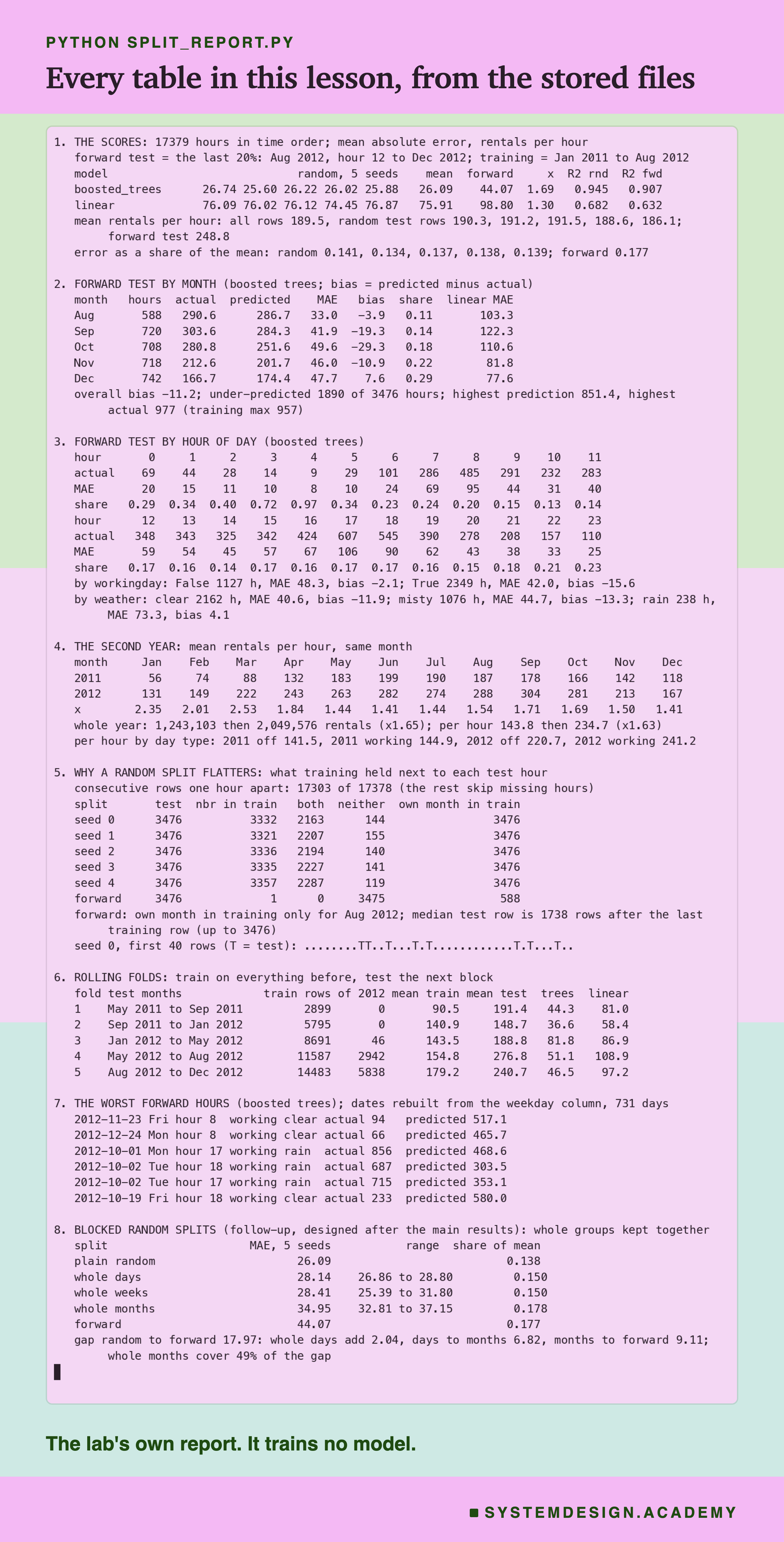
The report lives in scripts/labs/prodbreaks/split_report.py. It reads the lab's stored results, results/split.json, and the Bike Sharing data itself from scikit-learn's local copy, for the month, hour and other columns of each row. It trains no model. To find which rows each random seed put in training, it draws the same five splits again from their seeds; drawing a split only shuffles row numbers. A json mode writes the numbers to results/sp-report.json, which the figures read.

Before it prints anything, it checks the files against each other. The stored real counts for the forward test must be the counts in the data, row for row. The forward MAE of both models is computed again from the stored guesses and must match the stored score. The rolling folds' row ranges must match a fresh TimeSeriesSplit. If anything differs, the report stops.

The demo mode checks the student script's stored run against split.json. The box mode writes the playground below and checks that it gives the same overall and monthly errors as the report.

This box has no model in it. It holds the 3,476 forward test hours in time order: the month, the hour of the day, whether it was a working day, the real count and the boosted trees' stored guess. It runs in your browser.

As it is, the box prints the forward MAE over all 3,476 hours (44.07) with the bias (-11.25, the report rounds it to -11.2), then the table by month from the month slides.

Try by_hour() to see the rush-hour peaks. Try worst(10) for the ten worst hours. The functions take a rule for which hours to keep, so you can cut the test your own way: mae(lambda i: WORKING[i] == 1) gives the working-day error and bias(lambda i: WORKING[i] == 1) shows it was mostly too low; mae(lambda i: HOUR[i] in (8, 17, 18)) gives the error on the three peak hours alone; mae(lambda i: MONTH[i] == 12 and WORKING[i] == 0) gives December days off. Every number you get is from the real guesses of the lab's model.

Loading. fetch_openml("Bike_Sharing_Demand", version=2, as_frame=True) downloads the data (or reads the local copy) as a pandas table. X is the 12 input columns and y is count, the answer.

The model. new_model builds a fresh model every time it is called, so the random-split model and the forward-split model never share anything. A ColumnTransformer turns the four word columns into number codes with an OrdinalEncoder and passes the eight number columns through unchanged. HistGradientBoostingRegressor(random_state=0) is the boosted trees, with default settings. make_pipeline joins the two into a pipeline, a chain of steps that always run in the same order, so that the same column handling runs when the model learns and when it guesses.

Scoring. score trains the model on the training rows only, guesses the test rows, and prints mean_absolute_error and r2_score against the real counts of the test rows.

The two splits. train_test_split(rows, test_size=0.2, random_state=0, shuffle=True) is the random split: shuffle, then hold back 20%. The forward split is plain list slicing: for training and for the test, where is 80% of the rows. That one line, slicing instead of shuffling, is the whole fix.

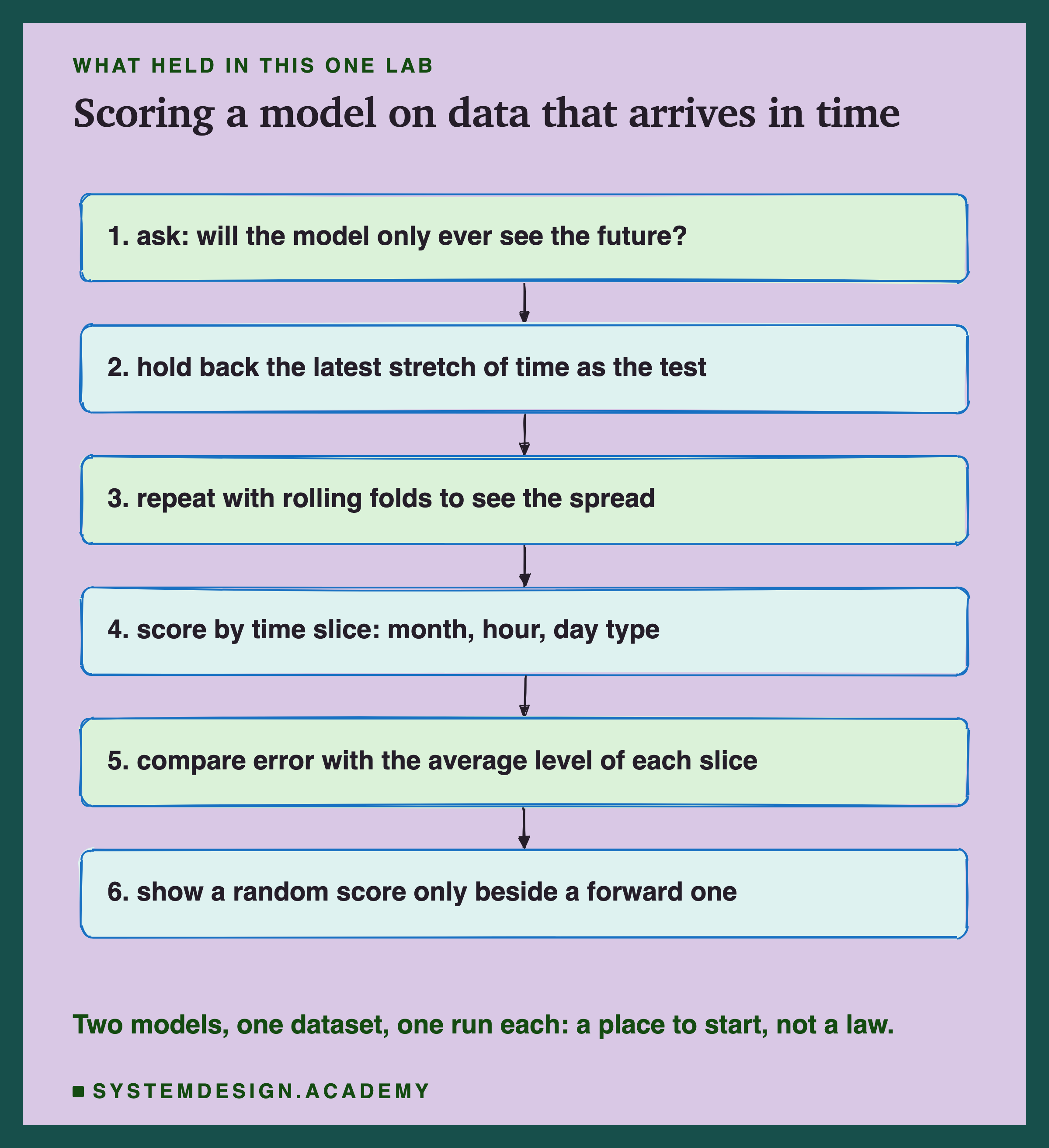
Ask when the model will be used. If every row has a time, and the model will only ever be asked about times after the data it learned from, then your test must look like that. This is true of demand forecasts, fraud scores, prices, sensor readings, and anything where the world changes and you retrain every so often.

Hold back the latest stretch as the test. Sort by time and cut. Train on everything before the cut, test on everything after. If you also tune the model's settings, hold back a second, earlier stretch for that, so the final test stays untouched.

Roll the split forward. One cut gives one future. Use TimeSeriesSplit or your own loop to test on several later stretches, and report the spread, not only the average. Here the trees ranged from 36.6 to 81.8 across five stretches.

Score by time slice. Break the error down by month, by hour, by kind of day, by whatever your users care about. The overall number hid that September and October were too low and that December's error was 29% of its average.

Compare the error with the level. If the future is busier or quieter than the past, the raw error moves for that reason alone. Report the error as a share of the average next to the raw error.

Keep the random split only as a comparison. It is still useful for one thing: the gap between the random score and the forward score is a measure of how much your model leans on nearby time. Never report the random score alone as what users will see.

Use a forward split when rows have a time and the model will be used on later times. Demand, traffic, prices, sales, fraud, anything with a clock. Here the random split promised a miss of about 26 bikes an hour; the future gave 44.

Use it when nearby rows are alike. Hours next to each other, readings from the same machine a minute apart, messages from the same customer in one week. A random split puts some of each cluster (a group of rows that are alike because they come from the same time or the same source) on both sides, so the test partly checks what the model saw of that group. Here, holding out whole days cost 2.04 and whole months 8.86. The same idea applies to groups without time: if you have many rows per customer and the model will meet new customers, hold back whole customers (scikit-learn's GroupKFold does this).

Use rolling folds when you need to know how much the score moves. Before you promise a number to anyone, see how it varies across several stretches of time. One forward split can land on an easy stretch or a hard one.

A random split is fine when the rows really are independent and the future looks like the past. For example, sorting photos of objects where each photo was taken separately and new photos will come from the same kind of camera and the same kind of scene. Even then, check how the data was collected: rows that look independent are often not.

A forward split is not a cure for a changing world. It tells you honestly how the model does on one stretch of the future. It cannot make a model trained on 2011 know about the growth of 2012. What it does is make sure you find out in testing rather than in production. The later lessons of this chapter are about what to do next: watching the inputs, measuring drift (how far new data moves away from the data the model learned from), and retraining.

Not a reason to throw away the random score. Report both. The gap between them is information: here it said that the model leaned heavily on having seen the same month of the same year.

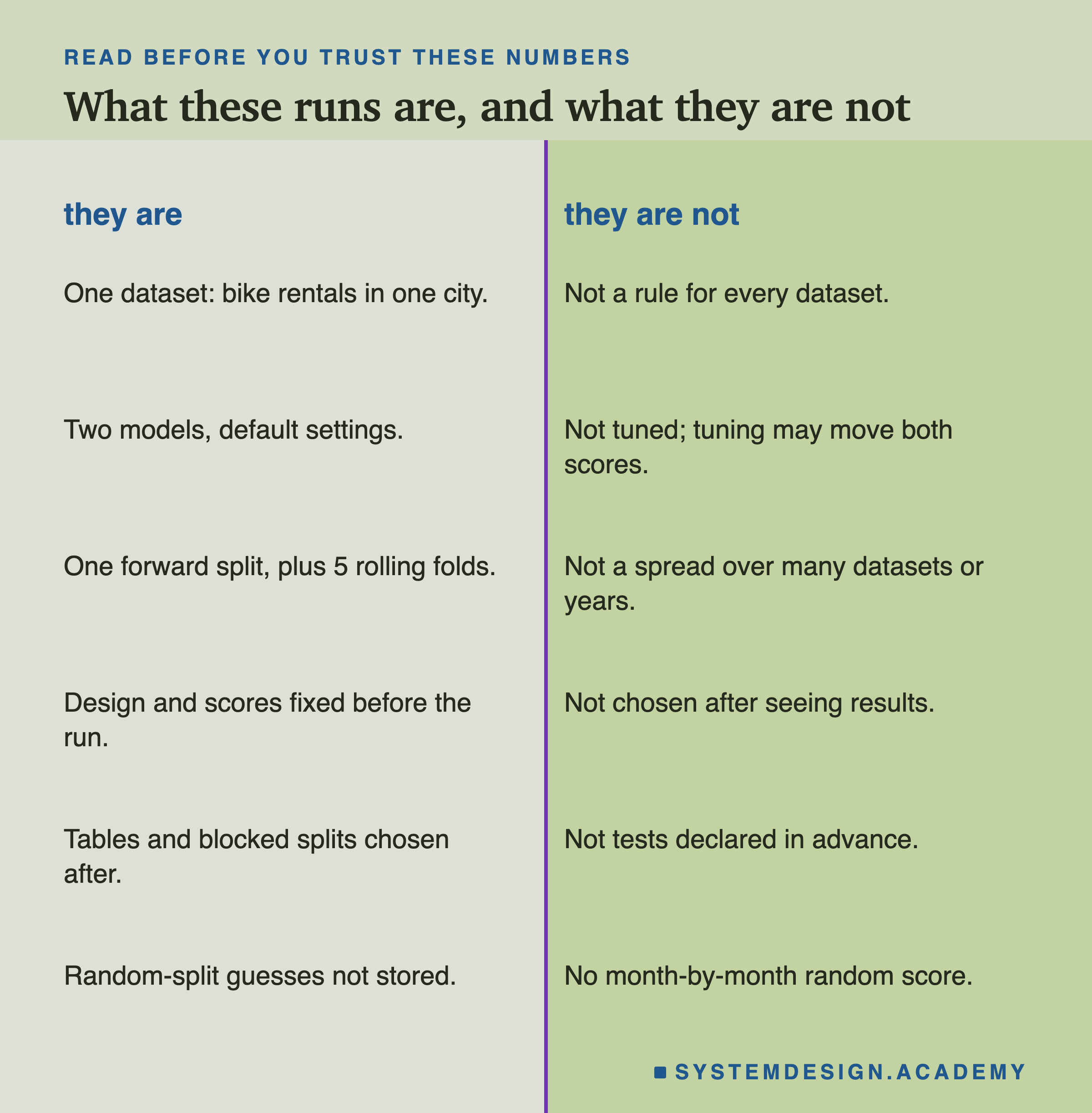
One dataset. Hourly bike rentals in one city over two years. The size of the gap, 1.69 times here, depends on how much the data changes over time and how alike neighbouring rows are. On other data it could be smaller or much larger. I make no claim that it is 1.69 anywhere else.

Two models, default settings, one run each. I did not tune either model. A tuned model might score better on both splits; nothing here says whether the gap would grow or shrink. The boosted trees use a fixed seed, so a rerun gives the same numbers, which the student script confirmed.

One forward split, plus 5 rolling folds. The forward test is one stretch of the future, the last four and a half months of 2012. The rolling folds show that another stretch can give a very different score, from 36.6 to 81.8 for the trees.

The design was declared; the reading was not. The splits, the models, the scores and the ratio were written in split_lab.py before the run. The tables by month, hour, working day and weather, the comparison of the years, the neighbouring-hour counts, the rebuilt dates, the blocked splits (a follow-up prompted by a review), the share of the average and every example were chosen after I saw the results. Read them as a description of this run, not as tests I set out to pass.

The random-split guesses were not stored. The lab kept the guess for every forward test hour, but only the scores for the random splits. So I cannot show the random split's error on late 2012 alone, which would be the cleanest comparison of the two splits on the same hours. I say so instead of rerunning the lab and changing its design after the fact.

The reasons are guesses. The low guesses in September and October line up with the months where 2012 differed most from 2011. That the model reasoned that way is my reading, not something the data proves.

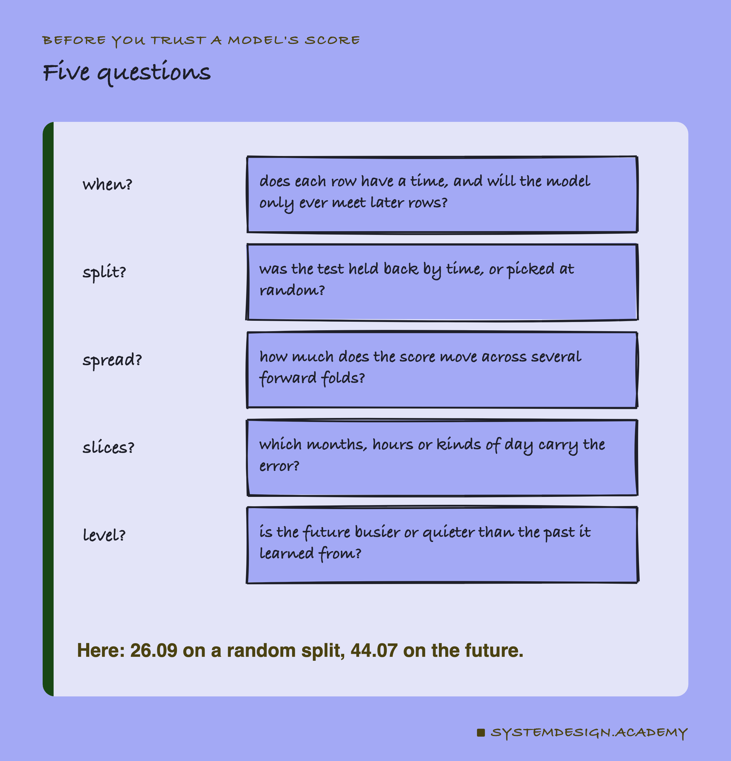
Take any model you or your team has scored in the last year, and find the line that made the test set. If it shuffles rows that have a time, change it to a cut in time and run the score again. Then run it on three or four later cuts and write down the spread. Then break the error down by month. It takes an afternoon, and you will know the number your users are going to see before they see it.

If the forward score is much worse, that is not a failure of the work. It is the first honest number, and it tells you where to look next. In this lab it pointed straight at the second year being busier than the first, which is exactly what the next lesson of this chapter studies: training on 2011 and scoring month by month into 2012, to watch a model grow old.