Which Ruler Do You Pick Up?
Let me start with a small picture.
Imagine you want to know how busy a small café is. You could count the customers who came in during the last hour. You could count the last week. Or you could count the whole year. Each count is true. Each one answers a slightly different question.
The last hour tells you about right now, but it is often zero, and zero tells you very little. The whole year almost never says zero, but it mixes this week with last winter. Somewhere in between there is a count that is most useful for the question you actually have.
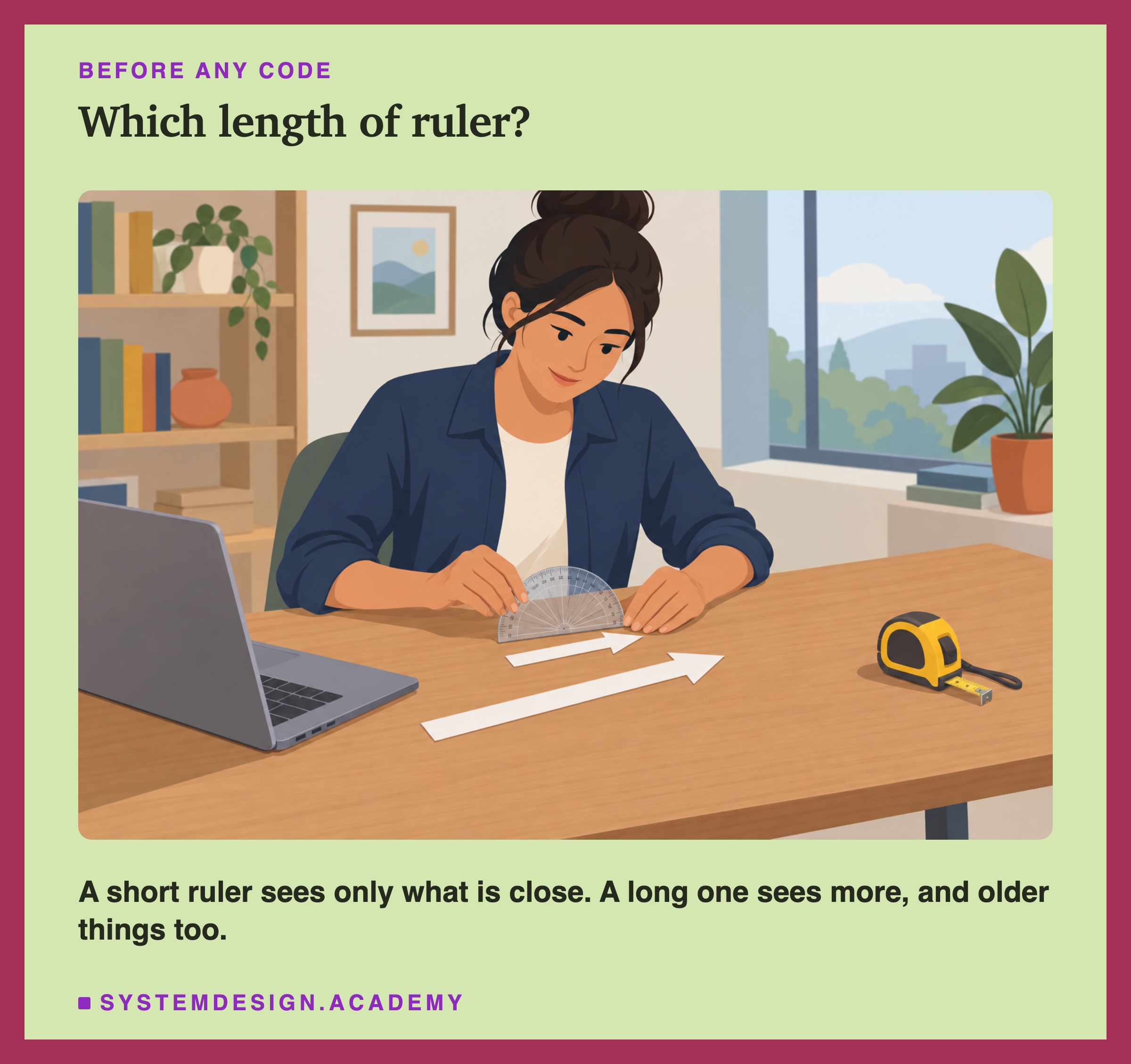
Machine learning teams face this choice every day. They write a feature like "purchases in the last 7 days" and then someone asks: why 7? Why not 30, or 90, or a year? Usually the answer is a guess, or a habit from the last project.
In this lesson I stop guessing. I measure six different lengths of ruler on real data from a real shop. Then I measure what happens when the model gets all of them at once.
Where This Lesson Starts
This lesson uses the same shop, the same customers and the same question as the rest of the chapter. If any of that is new, please read what a feature is first. It sets up the data and the task, and it built six simple features that I reuse here.
The six features from that lesson were recency, frequency, money, return share, tenure and products. Three of them, frequency, money and products, count over the customer's whole history before the cutoff. They have no window at all. They look back as far as the data goes.
The lesson on point-in-time joins showed what happens when a feature sees past the cutoff by mistake. Every window in this lesson ends strictly before the cutoff, and the code checks that, so that leak cannot happen here.
So the question is new. Lesson 1 asked whether features are worth more than a better model. This lesson asks a narrower question that comes right after. Once you decide to count things, over what stretch of time should you count them? And does it help to count over several stretches at once?
The Words You Need First
Please read this slide slowly if any word is new. Every slide after it uses these words.
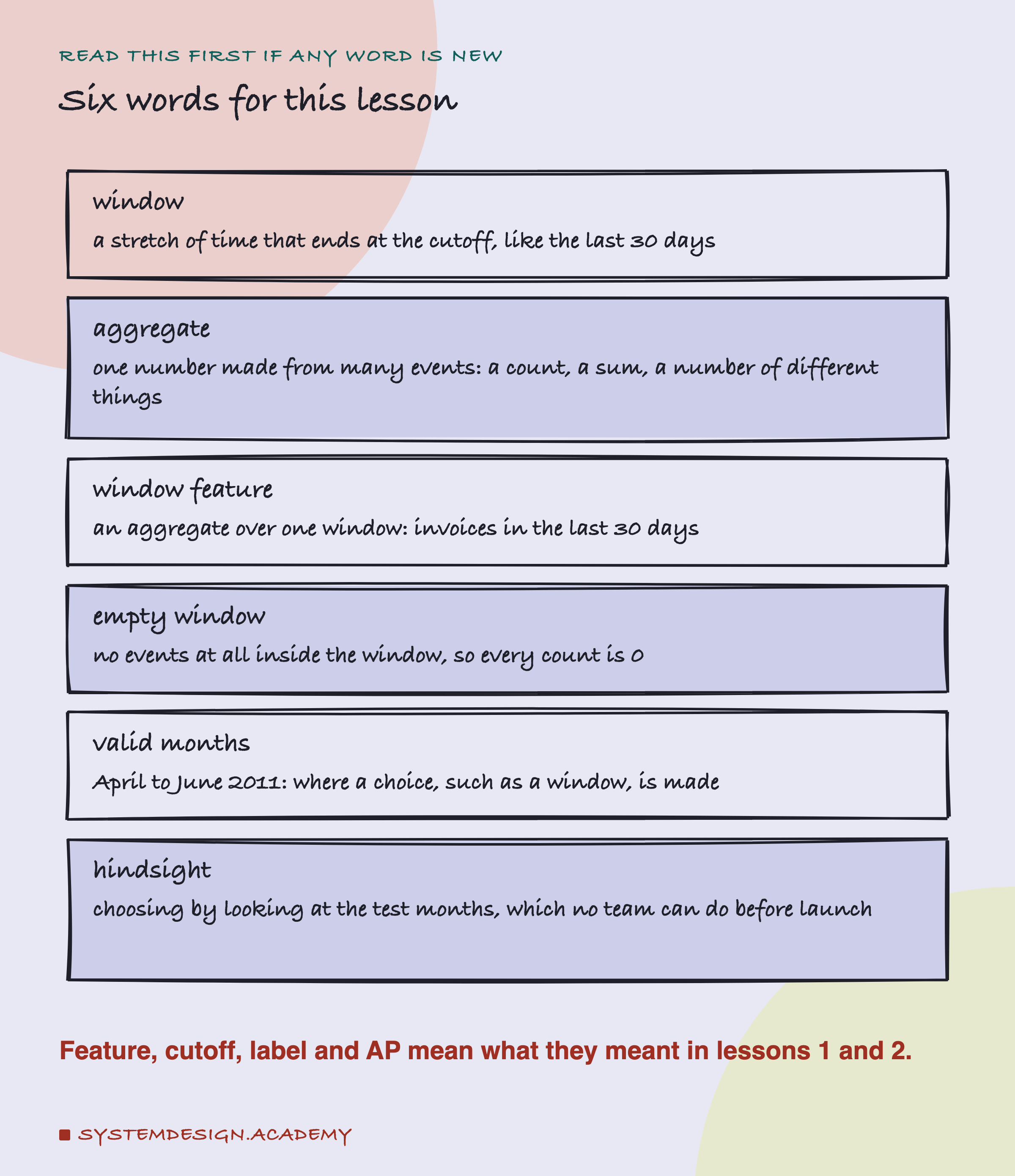
Window. A stretch of time that ends at the cutoff. "The last 30 days" is a window of 30 days. The cutoff is the moment we predict from, the first of a month here, and the window looks back from it.
Aggregate. One number made from many events. A count is an aggregate, and so is a sum or "how many different products". The word only means "gathered together".
Window feature. An aggregate over one window, such as "invoices in the last 30 days". Teams often call these rolling features, because each day the window rolls forward by one day.
Empty window. A window with no events inside it. Every count is then 0, and every sum is 0.
Valid months and hindsight are explained on the slides where they matter. Feature, cutoff, label and average precision (AP) mean exactly what they meant in lessons 1 and 2.
ROC-AUC. Pick one real buyer and one customer who did not buy, at random. ROC-AUC is the chance that the model gives the buyer the higher score. A coin flip gives 0.5 and a perfect model gives 1.
Seed. A number that fixes the random choices inside training, so a run can be repeated exactly. Changing the seed shows how much of a result is luck.
One Customer Through Six Windows
Here is one real customer, number 12349, at the cutoff 1 July 2011. Lesson 1 used the same customer, chosen there by a fixed rule, so you can compare the two lessons.
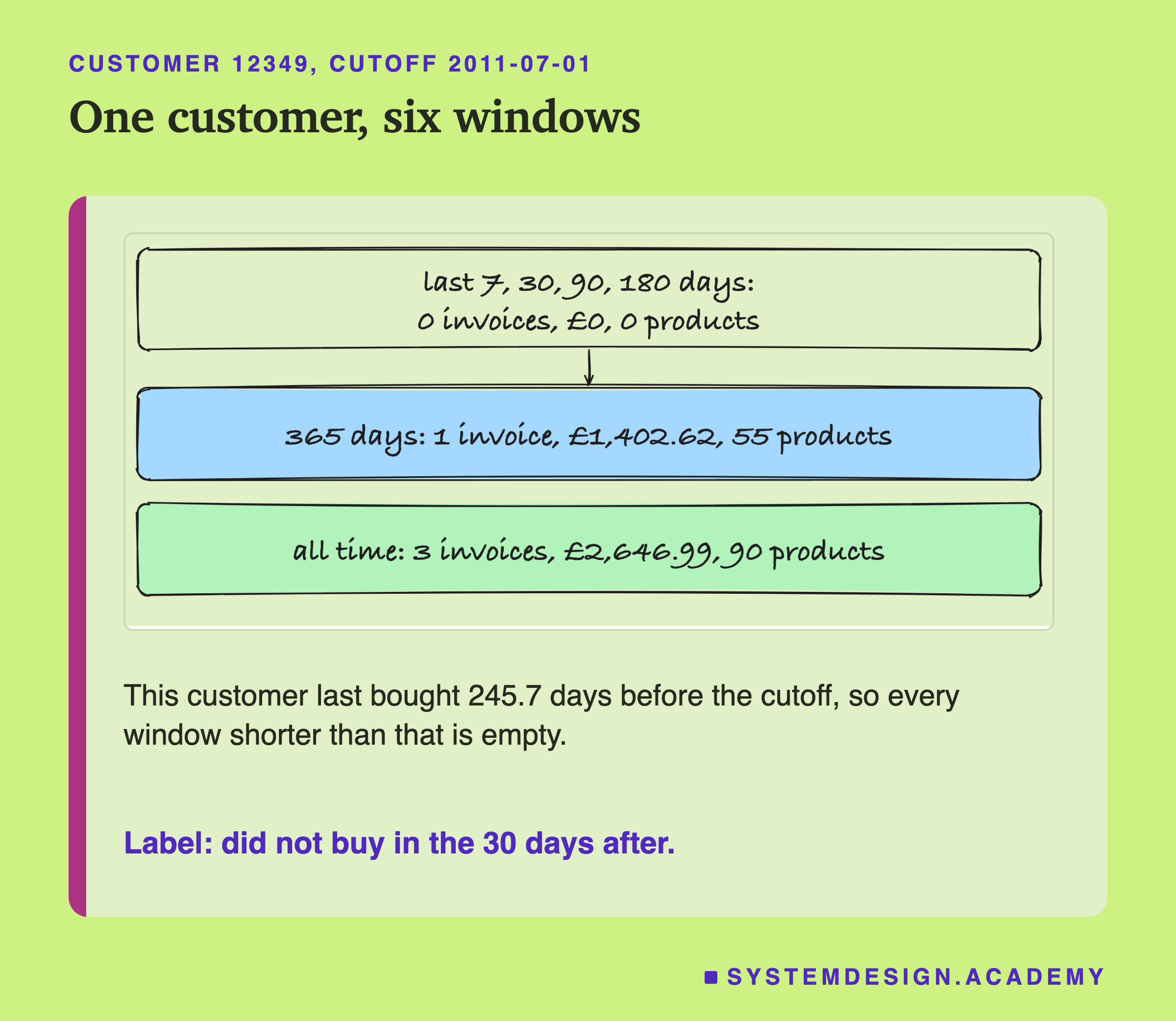
For each window I count three things from the customer's events before the cutoff. How many purchase invoices? How much did they spend after returns? How many different products did they buy? An invoice is one order.
This customer made 3 purchases in total, the last one 245.7 days before the cutoff. So the windows of 7, 30, 90 and 180 days are all empty: 0 invoices, 0 pounds, 0 products. The 365-day window holds 1 invoice worth £1,402.62 with 55 products. All time holds all 3 invoices.
Notice what the short windows lose. For this customer, the 7-day window says the same thing as it says for a customer who has never been active at all. Only the longer windows can tell the two apart.
This customer did not buy in the 30 days after the cutoff.
How Many Rows Each Window Can See
One customer is a story. The lab also counted every test row, so here is the same idea for all of them.
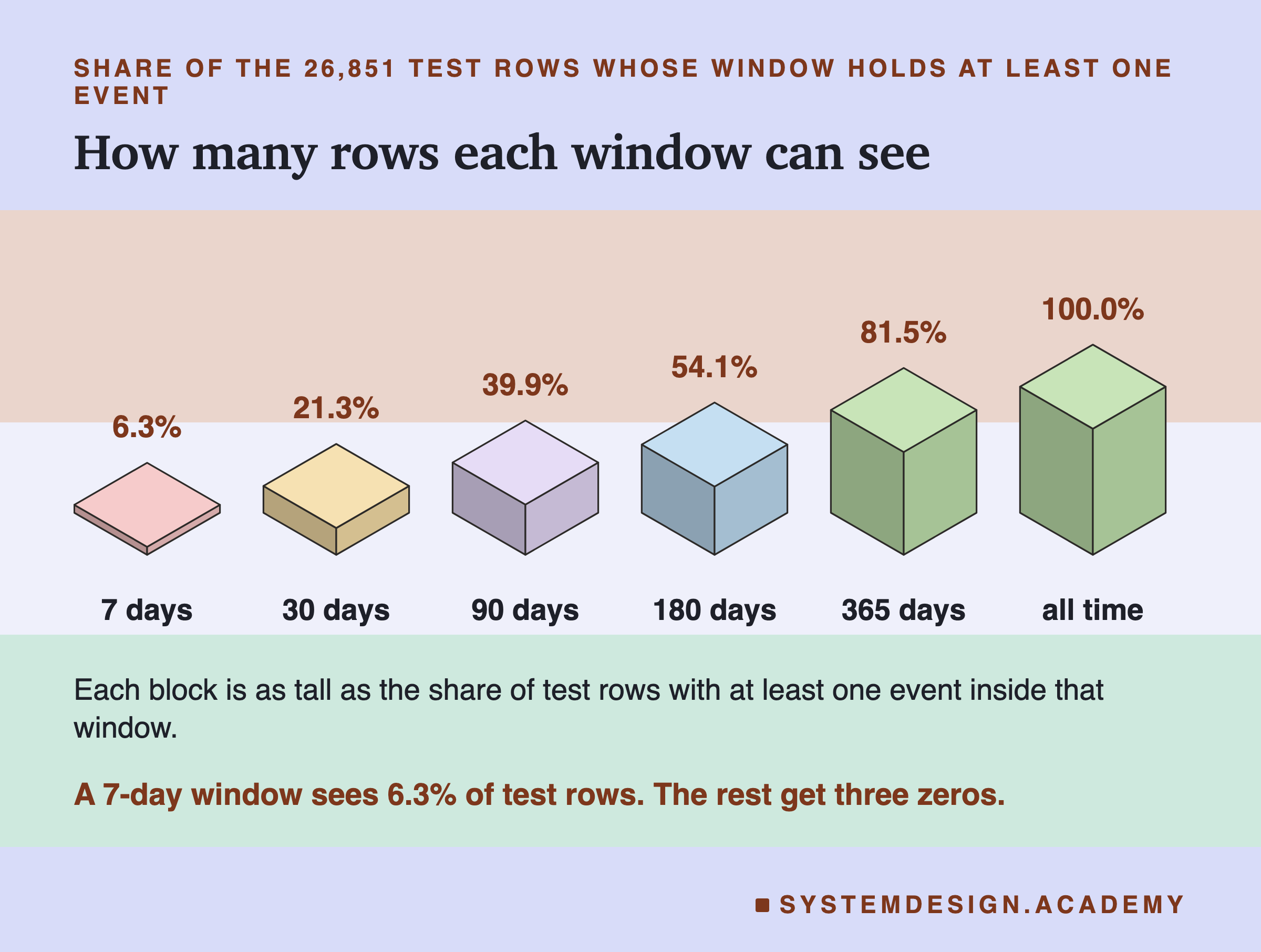
Of the 26,851 test rows, 93.7 percent had an empty 7-day window. For the 30-day window it was 78.7 percent, for 90 days 60.1 percent, and for 180 days 45.9 percent. So 180 days was the first window to see more than half of the rows. The 365-day window saw 81.5 percent: 18.5 percent of rows were empty there. All time is never empty, because every customer in the task has bought or returned something before the cutoff.
Why are short windows so empty? This shop mainly sells gift items, and many of its customers are wholesalers, people who buy to sell again. The counts show that most customers simply did not order in any given week.
This matters for a model. When nine rows in ten have the same three zeros, the model cannot tell those customers apart using that window. A short window can still be useful, but it can only speak about the few customers who were active very recently.
The Shop, the Task and the Split
The data is UCI Online Retail II, a public dataset under a CC BY 4.0 licence. It holds every sale of a UK online shop from 1 December 2009 to 9 December 2011. The chapter's fixed cleaning drops lines with no customer id and keeps returns as flagged rows. A return is an invoice whose number starts with "C", and its amount is negative.
The task is the chapter's fixed one. On the first of each month, for every customer seen before that day, will they buy in the next 30 days? Each pair of a customer and a cutoff is one row.
The rows are split by time. Train months, March 2010 to March 2011, give 44,521 rows; the models learn from these. Valid months, April to June 2011, give 14,673 rows; any choice is made here, such as which window to use. Test months, July to November 2011, give 26,851 rows; they only score, and they choose nothing.
The average share of buyers over the five test months is 0.196. A model that ranks customers at random gets an AP near that number, so 0.196 is the floor to beat.
How a Window Is Cut, and Checked
All the events sit in one table, sorted by time. Take a cutoff T and a window length W. The code needs the events from T minus W up to, but not including, T.
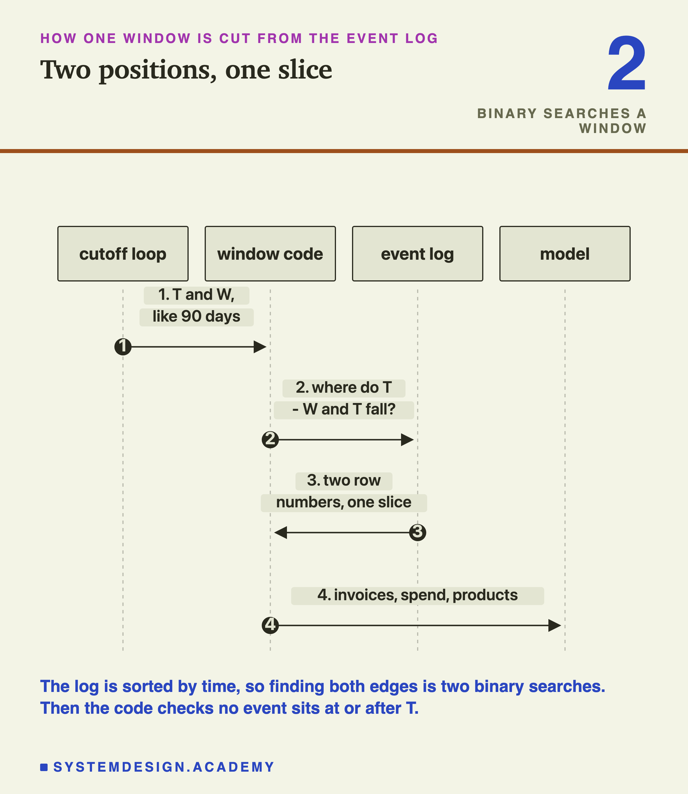
Because the table is sorted, the code does not scan every row. NumPy's searchsorted finds the first row at or after T minus W, and the first row at or after T. A binary search like this halves the table again and again until it lands on the right row, so it is very fast. Everything between the two positions is the window.
The code then checks two things for every cutoff and every window. No event in the slice is at or after the cutoff, and no event is before the window's start. If either check fails, the lab stops with an error instead of printing a number.
There is a third check. The all-time window counts the same things as lesson 1's frequency, money and products. So the lab asserts that, for every row, they are equal. They are. That is a cheap way to catch a bug in the window code, because the old code was already checked.
How the Lab Was Built
I wrote the lab's design into the docstring of scripts/labs/features/window_aggregations.py before it first ran. Lesson 1's lab and its results already existed, and I had read them. No model had been trained on any window feature yet.
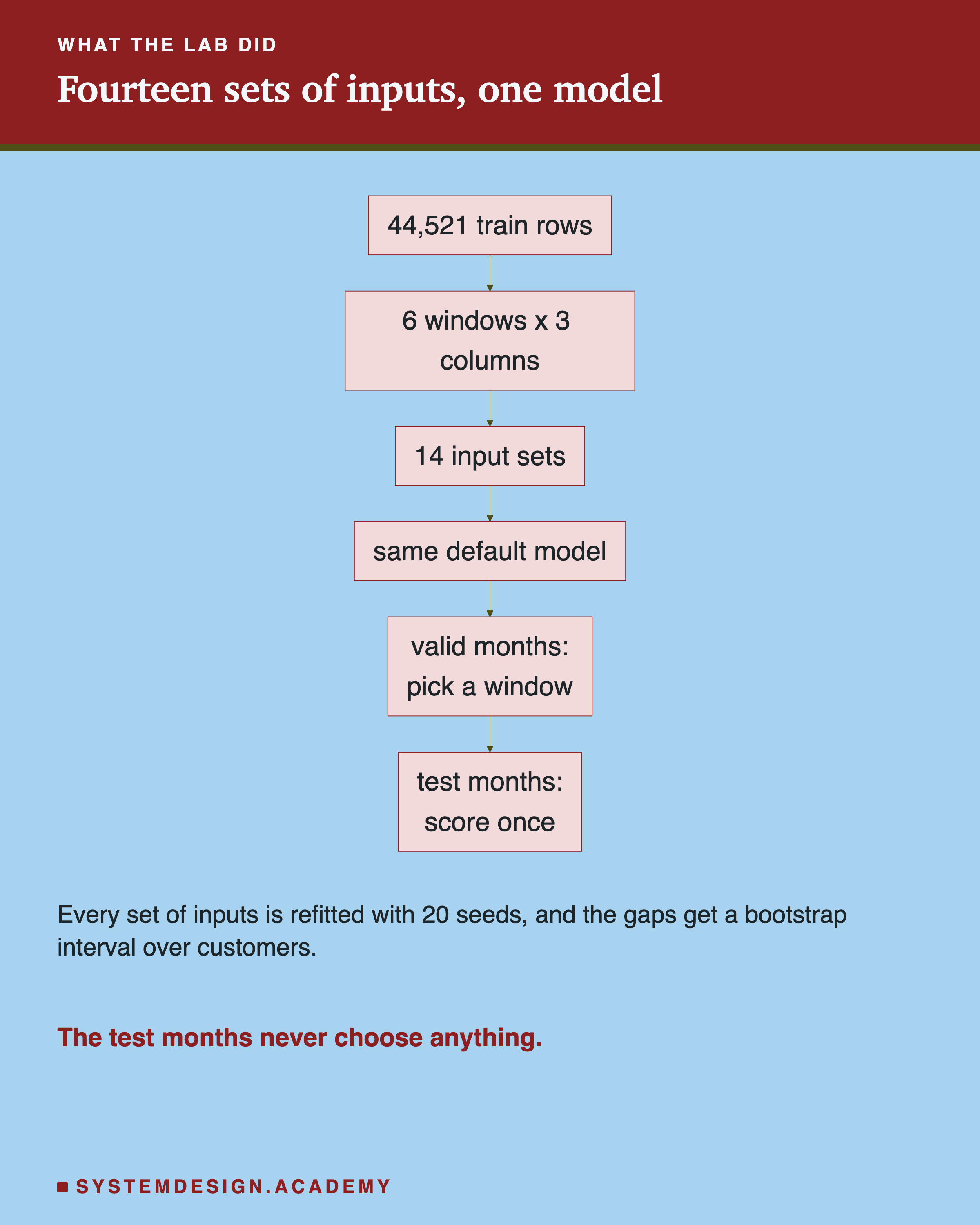
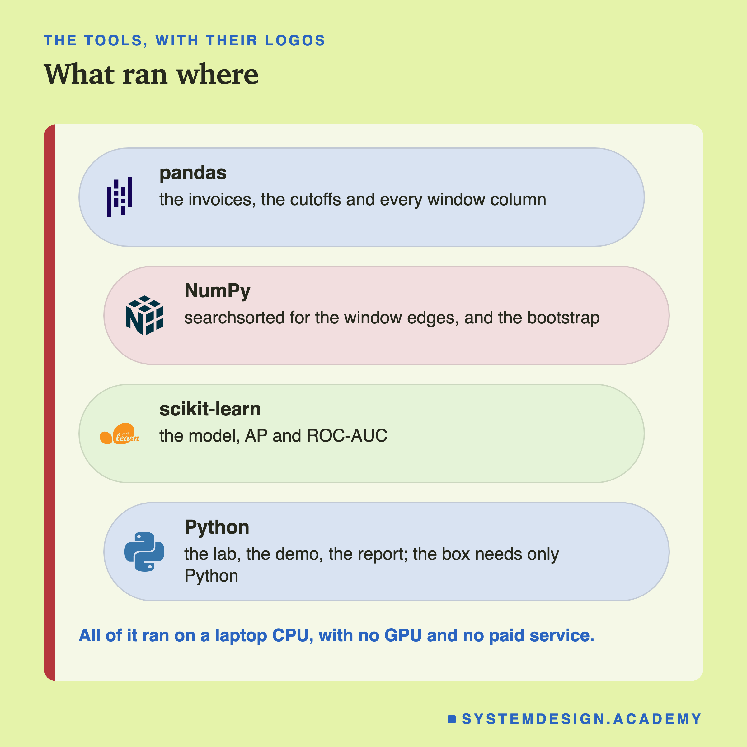
The model is the same as in lesson 1: scikit-learn's HistGradientBoostingClassifier with its default settings and random_state=0. It builds many small decision trees, each one fixing the mistakes of the trees before it. Only the inputs change from one contestant to the next. That keeps the comparison fair.
The design also wrote down four guesses, so they could be wrong in public. Here they are, scored against the results.
-
Longer windows beat 7 days, with 365 days or all time the best single window. Half right. Longer windows did beat 7 days. But the valid months picked 180 days, and all time came 4th of the six.
-
All windows together beat the best single window by a little. Right: +0.0230.
-
Lesson 1's six beat all the windows. Wrong: all windows scored higher. A later slide explains why this race was not quite what it looks like.
-
The six plus the windows cannot be told apart from the six. Wrong: +0.0161, with an interval from +0.0106 to +0.0218, and 5 of 5 months.
The lab must also reproduce a number from lesson 1 before it reports anything. The six made features on the default model scored a mean test AP of 0.5450 there. Here they scored 0.5450 again, equal to twelve decimal places. If they had not, the run would have stopped.
Fourteen Contestants
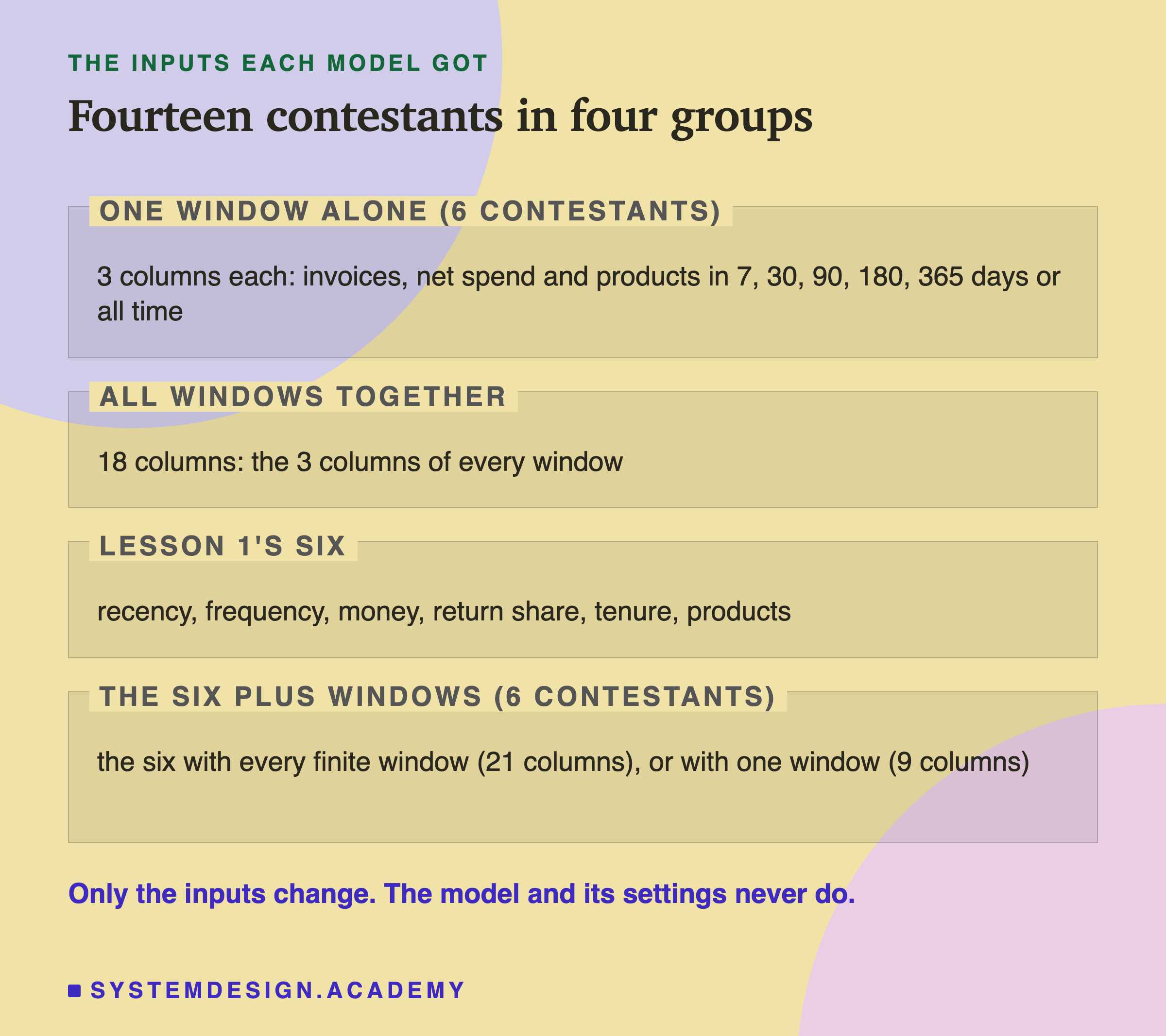
One window alone. Six contestants, one per window: 7, 30, 90, 180 and 365 days, and all time. Each gets 3 columns.
All windows together. One contestant with all 18 columns. The model can then weigh short and long windows against each other by itself.
Lesson 1's six. The six made features, built with lesson 1's own code. This is the reference row.
The six plus windows. One contestant gets the six plus all five finite windows, 21 columns. I left out the all-time window there, because its three columns are exactly the six's frequency, money and products. Five more contestants get the six plus one window each, 9 columns. I declared those five before the run, so "which one window should I add to the features I already have?" was a planned question, not one I asked after seeing results.
Each contestant is scored on the valid months and on the test months.
The Lab's Report, Running
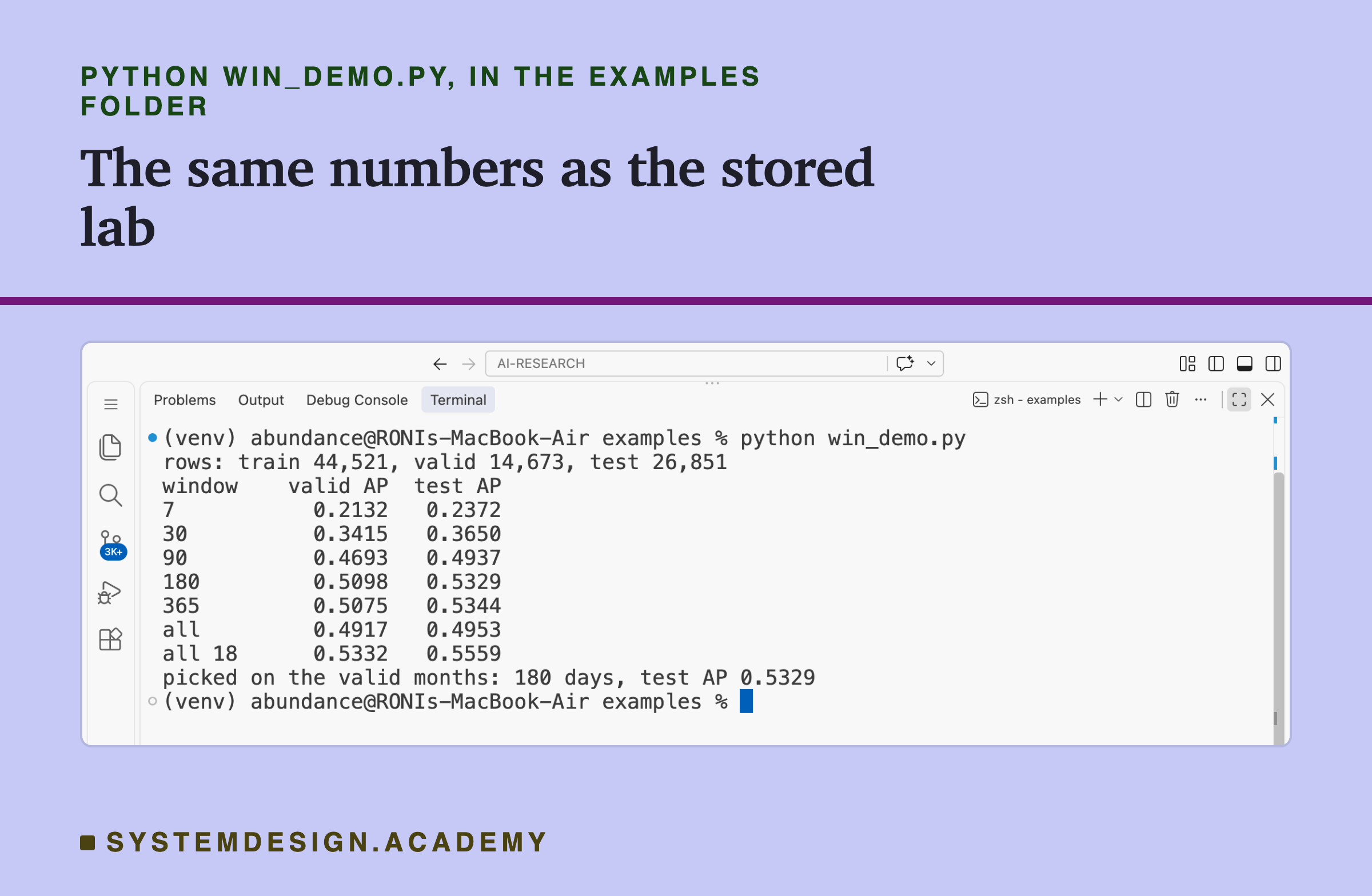
This is a real recording of the report script, win_report.py, on the laptop where the lab ran. It does not train anything. It reads the stored results and checks every number this lesson uses.
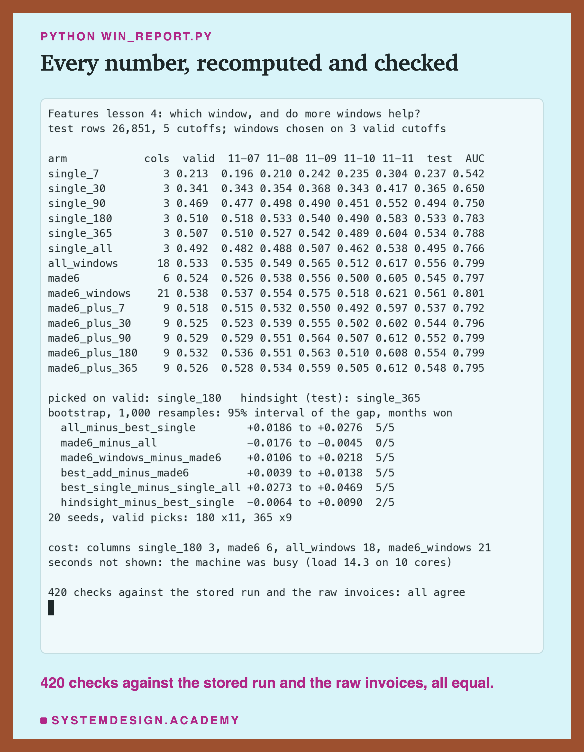
The report checks each mean against the per-month numbers it came from, and each bootstrap interval against the 1,000 stored resamples. It also rebuilds the window columns from the raw invoices with its own, simpler code: it filters the table instead of using searchsorted. From those it recomputes the share of empty windows, the buy rates, the correlations and customer 12349's values, and checks each one against the lab.
It also checks three more things. The student demo printed the same numbers as the lab. The playground box prints what it should. And every number in this lesson appears in the lesson text. If anything disagrees, it exits with an error.
One Window at a Time
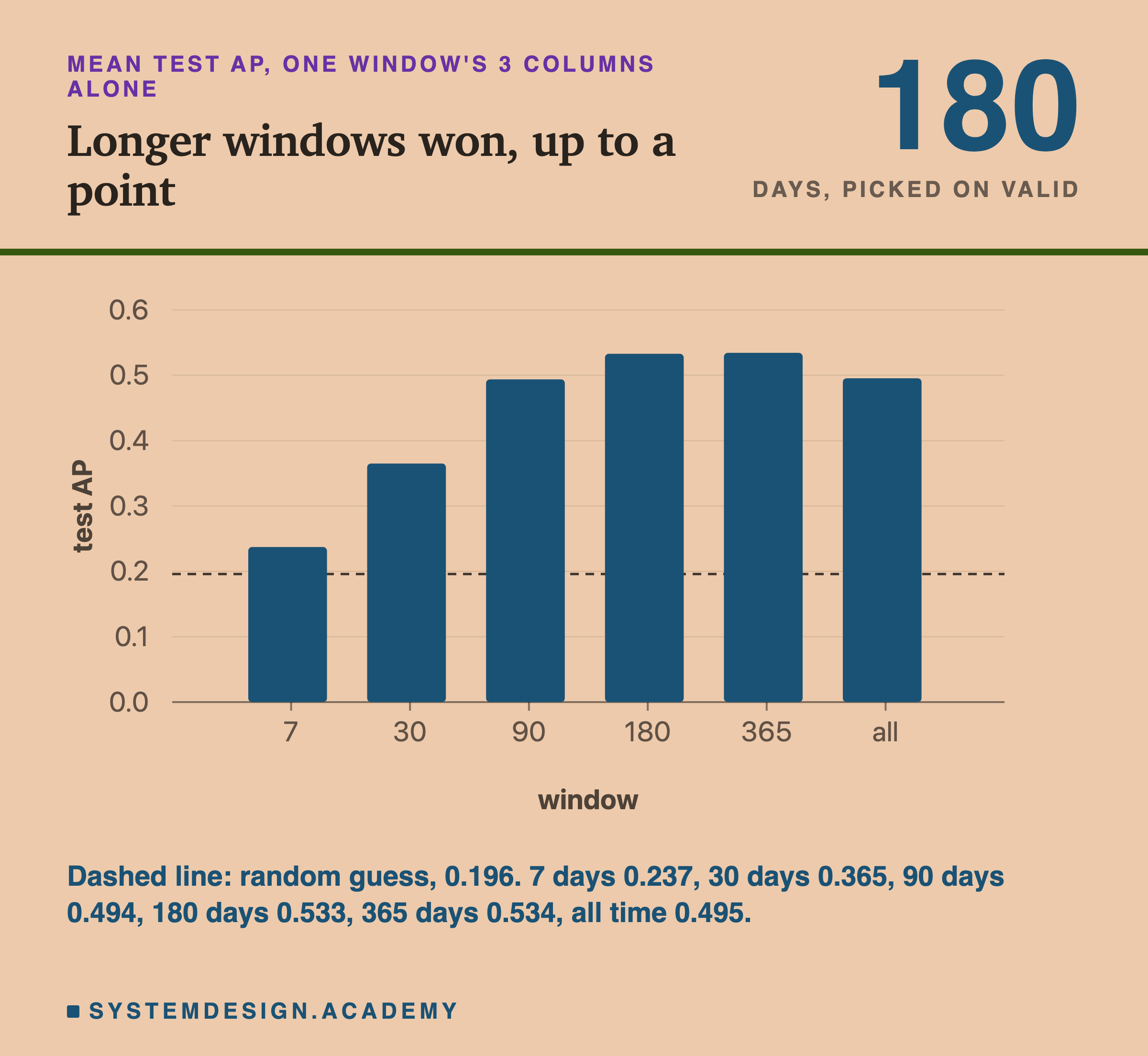
Here is each window alone, scored on the five test months. Each model saw 3 columns and nothing else.
| window | valid AP | test AP | test ROC-AUC |
|---|---|---|---|
| 7 days | 0.2132 | 0.2372 | 0.542 |
| 30 days | 0.3415 | 0.3650 | 0.650 |
| 90 days | 0.4693 | 0.4937 | 0.750 |
| 180 days | 0.5098 | 0.5329 | 0.783 |
| 365 days | 0.5075 | 0.5344 | 0.788 |
What an Empty Window Still Says
A fair question: if a window is empty, is that row useless? Not quite. The lab measured how often customers with an empty window still bought.
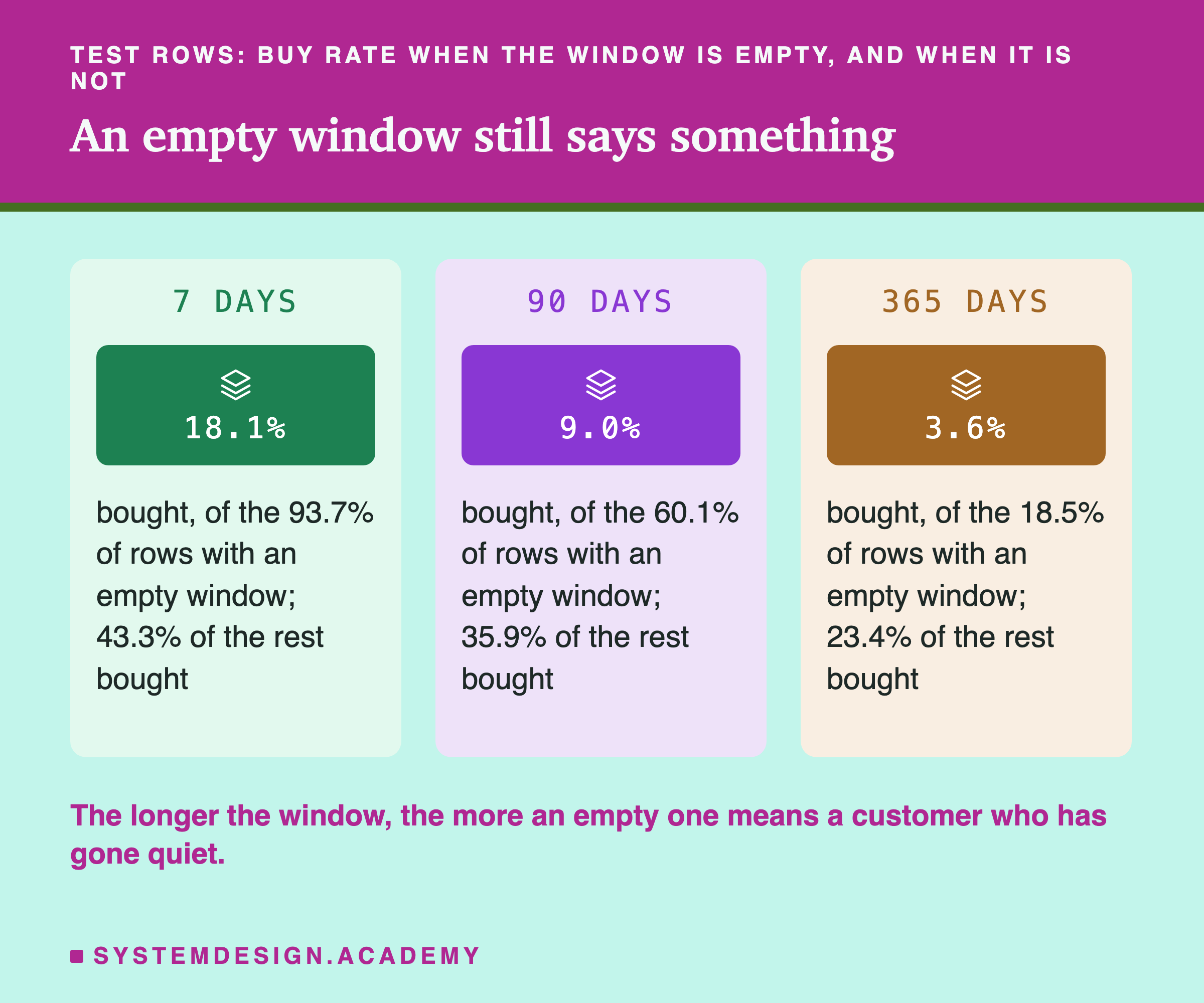
With a 7-day window, 18.1 percent of the customers with an empty window still bought in the next 30 days. That is close to the overall share, so "nothing in the last week" says very little. With a 365-day window, only 3.6 percent of the customers with an empty window bought. "Nothing in the last year" says a lot: this customer has very likely gone quiet.
So a long window says something even when it is empty. A short window mostly says something when it is not empty: 43.3 percent of rows with any activity in the last 7 days bought again.
This is why the two kinds of window can help each other. A short window picks out the few customers who are active right now. A long window sorts everyone else into "still around" and "gone". One window alone cannot do both jobs, and the next slides test whether the model can use both at once.
Choosing the Window Honestly
A team that wants one window has to choose it somehow. The honest way is to choose on the valid months, then report the test months untouched.
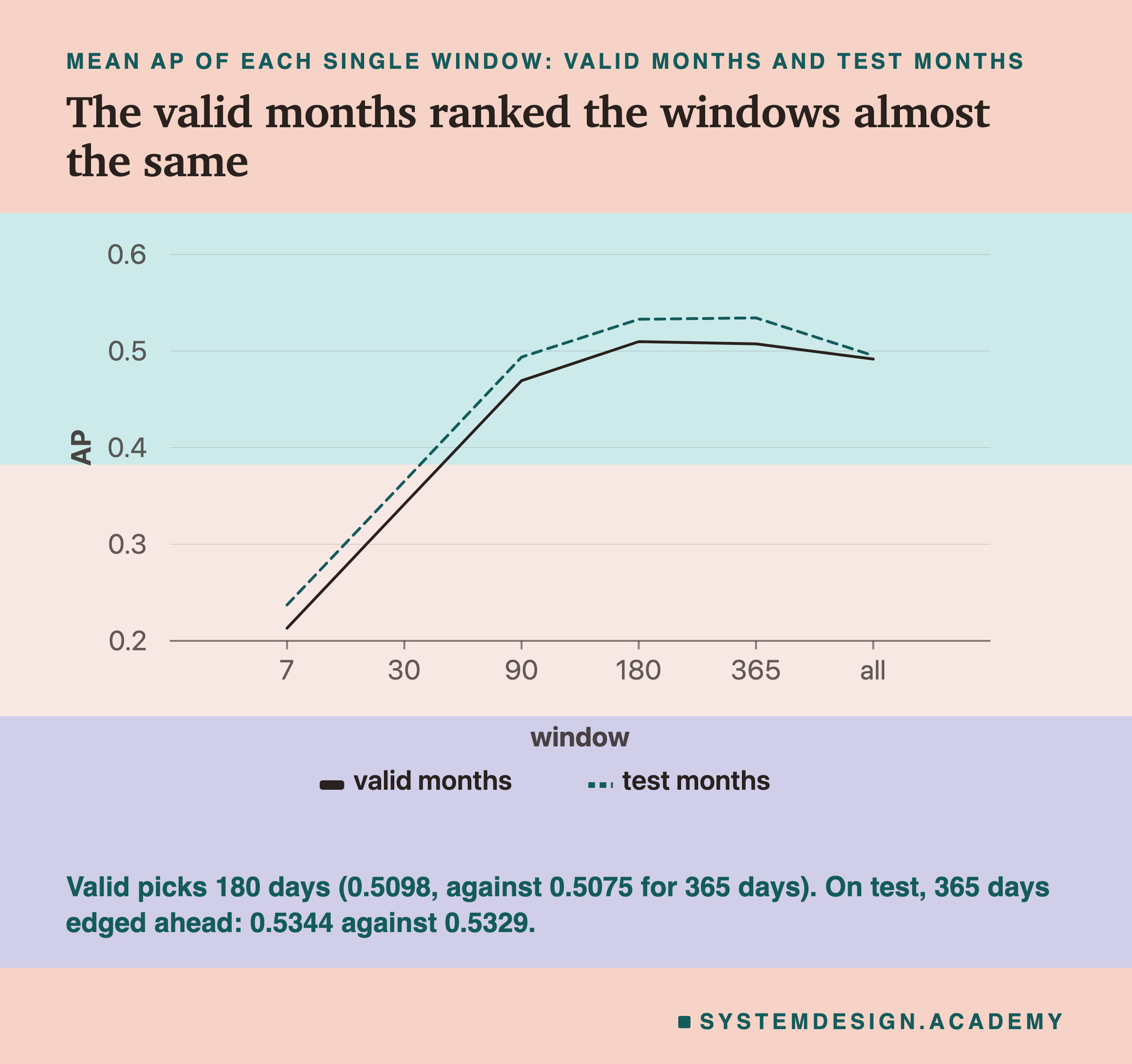
On the valid months, 180 days scored 0.5098 and 365 days 0.5075, so the valid months picked 180 days. On the test months, 180 days scored 0.5329.
If I had looked at the test months instead, I would have picked 365 days, at 0.5344. That is hindsight: choosing with knowledge a team cannot have before launch. I report it only for comparison, clearly labelled.
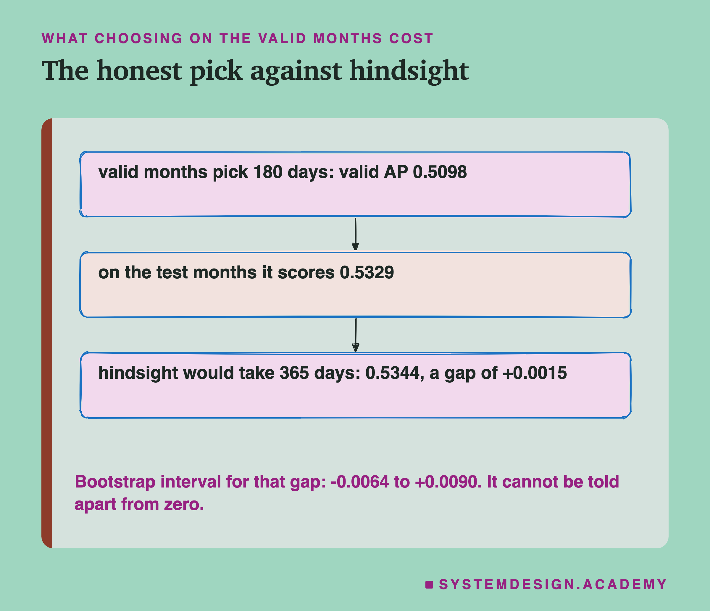
The gap between the honest pick and hindsight was +0.0015. The 365-day window won 2 of the 5 test months against 180 days, and its bootstrap interval ran from -0.0064 to +0.0090. That interval includes zero, so this gap cannot be told apart from luck. Choosing on the valid months cost almost nothing here. The valid months put the windows in nearly the same order as the test months did. You can see it in how closely the two lines follow each other.
Do More Windows Help?
Now the second half of the question. What if the model gets more than one window?
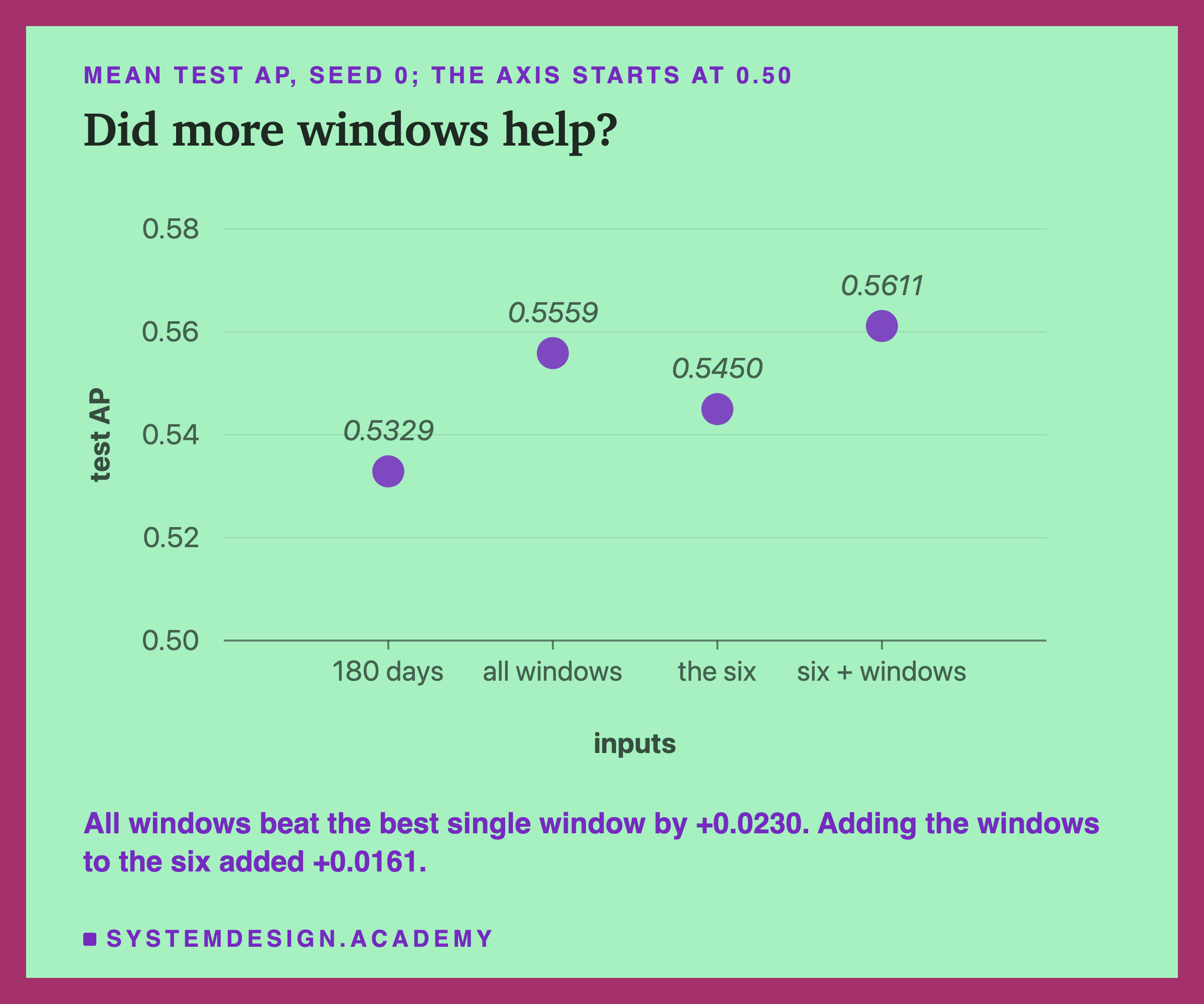
| inputs | columns | test AP | test ROC-AUC |
|---|---|---|---|
| 180 days alone | 3 | 0.5329 | 0.783 |
| lesson 1's six | 6 | 0.5450 | 0.797 |
| all windows | 18 | 0.5559 | 0.799 |
| six plus windows | 21 | 0.5611 | 0.801 |
Yes, more windows helped here, and by more than I expected. All 18 window columns together scored 0.5559, which is +0.0230 above the best single window. They won all 5 test months, and the bootstrap interval ran from +0.0186 to +0.0276.
The surprise was against lesson 1's six features. I guessed the six would win, because the windows hold no recency, tenure or return share. All windows scored 0.0109 higher, and the six won 0 of the 5 months. The interval for the six minus all windows ran from -0.0176 to -0.0045, entirely below zero.
Why Each Extra Window Adds Less
If several windows help, why not add a hundred? Because neighbouring windows mostly say the same thing.
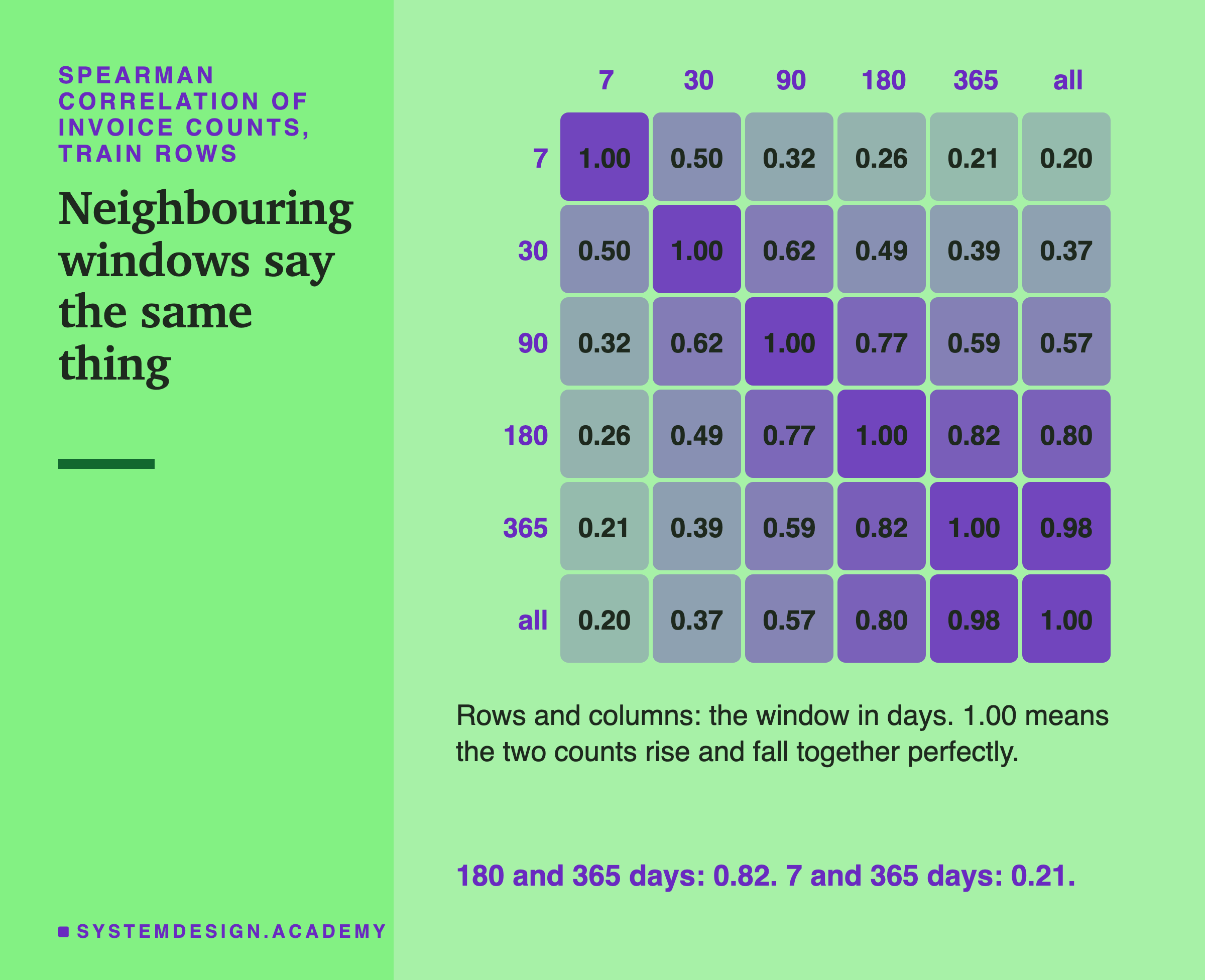
A correlation measures how much two numbers rise and fall together. The kind here, Spearman's, only looks at the order of the values, so it is not thrown off by a few customers with very large counts. 1.00 means the two orders agree perfectly, and 0 means they have nothing to do with each other.
The 365-day count and the all-time count had a correlation of 0.98: almost the same column twice. 180 and 365 days had 0.82. But 7 days and 365 days had only 0.21. Those two windows really do describe different things.
So the useful mix is a few windows that are far apart, not many that sit close together. A 90-day window next to a 120-day window adds a column the model mostly already has. I did not test a 120-day window, but the pattern in this grid points that way.
Which One Window to Add?
Many teams already have features like lesson 1's six. For them the practical question is: if I add only one window, which one?
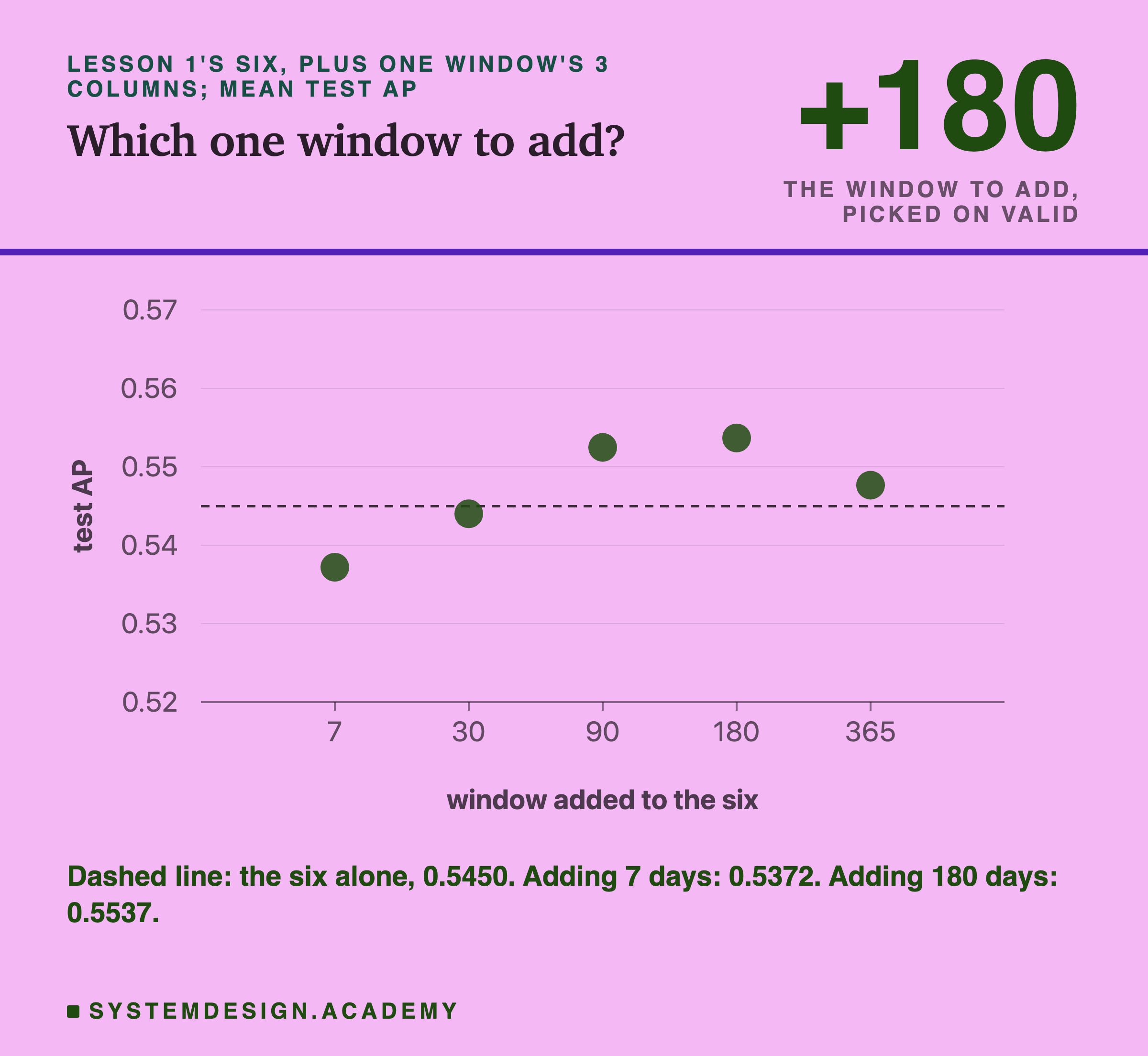
| added to the six | valid AP | test AP |
|---|---|---|
| nothing | 0.5235 | 0.5450 |
| 7 days | 0.5178 | 0.5372 |
| 30 days | 0.5253 | 0.5440 |
| 90 days | 0.5294 | 0.5525 |
| 180 days | 0.5323 | 0.5537 |
| 365 days | 0.5256 | 0.5477 |
The valid months picked 180 days, and on the test months it was also the best of the five. It added +0.0087 to the six, won 5 of 5 months, and its interval ran from +0.0039 to +0.0138.
How Sure Can I Be?
One run could be luck. I checked two kinds of luck, the same two as in lesson 1.
Luck in training. With more than 10,000 training rows, this model turns on early stopping by itself. It keeps 10 percent of the training rows aside, picked at random, to decide when to stop adding trees. That is a library default, and it is the randomness the seed moves. So I retrained every contestant with 20 seeds, 0 to 19.
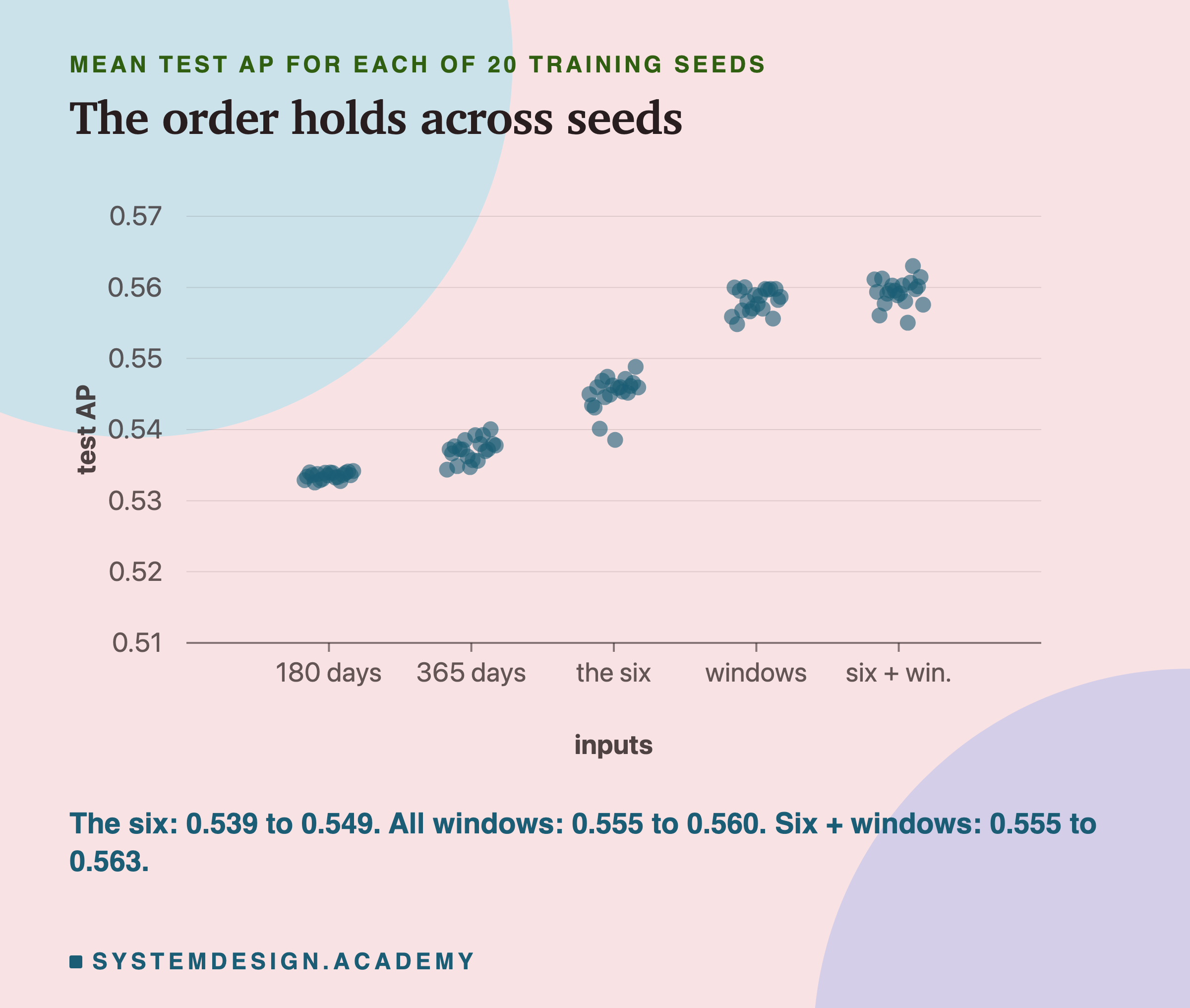
Over 20 seeds the six ranged from 0.539 to 0.549, all windows from 0.555 to 0.560, and the six plus windows from 0.555 to 0.563. The six never reached the window sets.
Luck in which customers were tested. A bootstrap draws the test customers again at random, with repeats allowed, 1,000 times, and works out each gap every time. The middle 95 percent of those gaps is the 95% interval.
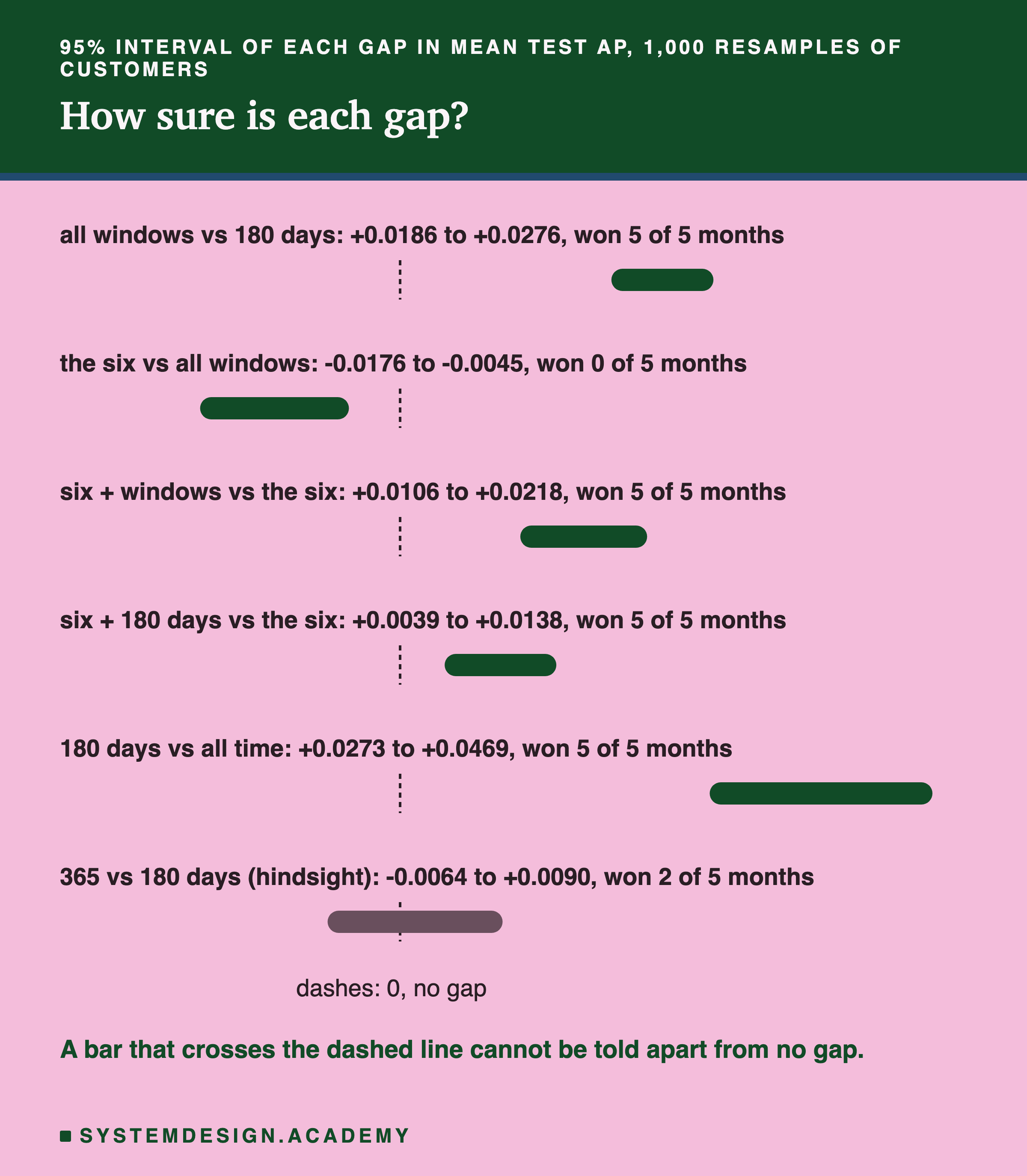
Five of the six intervals stay clear of zero. The one that crosses it is hindsight against the honest pick.
Is the Choice Itself Stable?
There is one more kind of luck that is easy to forget: luck in the choice. The valid months picked 180 days at seed 0. Would they pick it at every seed?
They did not. Over the 20 seeds, the valid months picked 180 days 11 times and 365 days 9 times. The two windows were so close on the valid months that the random part of training was enough to swap them.
On the test months, by contrast, 365 days was ahead of 180 days at every seed. 180 days ranged from 0.533 to 0.534, and 365 days from 0.534 to 0.540. So the valid months were a coin toss between two windows that were nearly level, and the test months leaned slightly one way.
What should a team take from this? When two windows are this close, the choice between them hardly matters for the score, and you should not build a story on it. Saying "180 days is the right window for this shop" would claim far more than the data shows. The safer reading is: something between six months and a year worked best alone, the short windows did not, and a mix beat any one window.
There is also a simple way out of the coin toss: do not choose. Give the model both windows, as the all-windows contestant did, and let it weigh them.
What Each Set of Inputs Costs
More windows are not free. Each window is more columns to compute, store and serve to the live app, and each one is one more thing that has to stay correct.
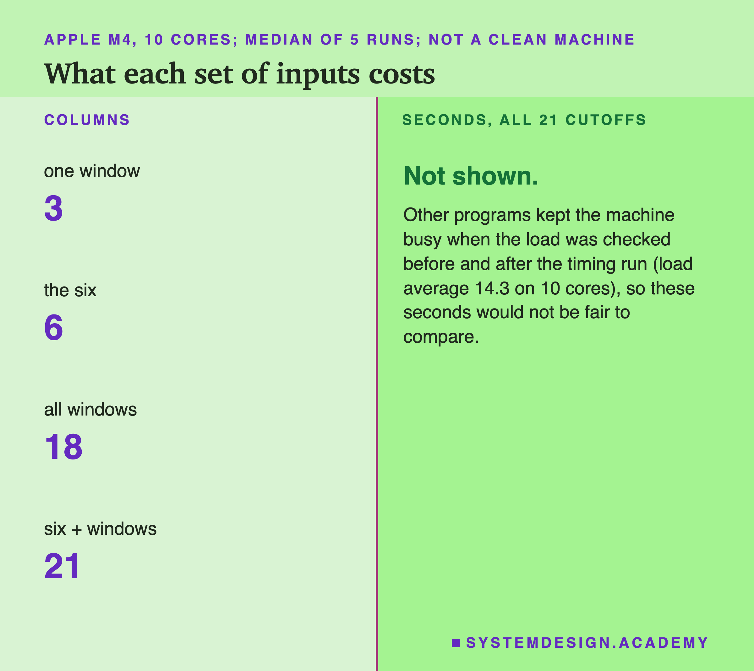
The column count is simple. One window is 3 columns. The six are 6. All windows are 18, and the six plus the five finite windows are 21. So the best contestant needed 7 times the columns of a single window, for a gain of 0.028 in AP over the best single window.
I also planned to measure how long each set takes to compute, on this laptop, with nothing else running. The design said a timing only counts if the machine is quiet. It was not: another lab was running on the same laptop. The load average, checked just before and just after the timing run, was 14.3 and 14.0 on 10 cores. So I do not report the seconds. I would rather give you no number than a number that mostly measures someone else's program.
What I can say without a clock: the window code reads each event once per window it falls in. A 365-day window covers far more rows than a 7-day one, so it costs more to compute. A real system pays that cost every night, for every customer.
The Lab's Code, Piece by Piece
The lab is one file, scripts/labs/features/window_aggregations.py. It imports lesson 1's feature code instead of copying it, so the six made features are guaranteed to be built the same way.
window_columns builds the windows. For each cutoff it finds the cutoff's row position once with searchsorted. Then for each window it finds the start position, and takes the rows in between with iloc. On that slice, groupby("customer_id") with nunique counts invoices and products, and sum adds the spend. Customers with no rows in the slice get 0 through reindex(...).fillna(0). The two leak checks sit right there, so a mistake fails at the place it happens.
joined merges lesson 1's tables and the window columns onto the label table. It uses validate="one_to_one", which makes pandas stop with an error if a customer appears twice. Then it asserts that the all-time columns equal lesson 1's frequency, money and products for every row.
fit_arm trains the default model on one set of columns. Every contestant goes through it, so the only thing that differs is the column list.
bootstrap redraws the customers within each test month and uses the same redraw for every contestant, so each gap is measured on the same customers. It stores all 1,000 gaps, which is how the report checks the intervals later.
Try It Yourself
The full lab trains 294 models and took about 16 minutes on my laptop while another lab shared it. I wrote a small demo that does the heart of it. It builds the six windows, trains one model per window and one on all 18 columns, and makes the choice on the valid months.
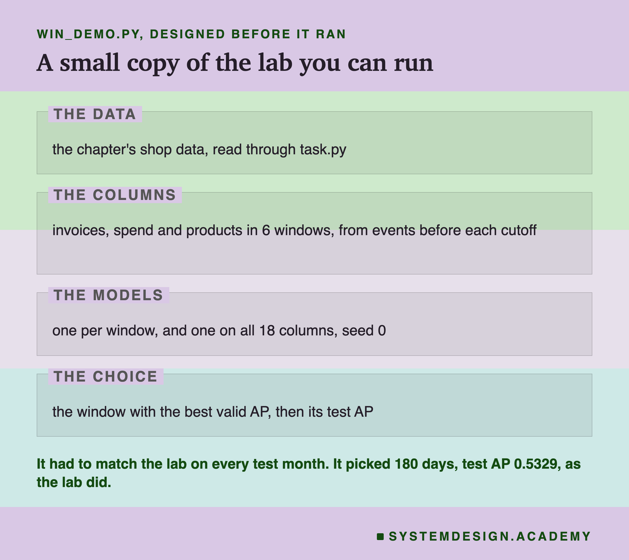
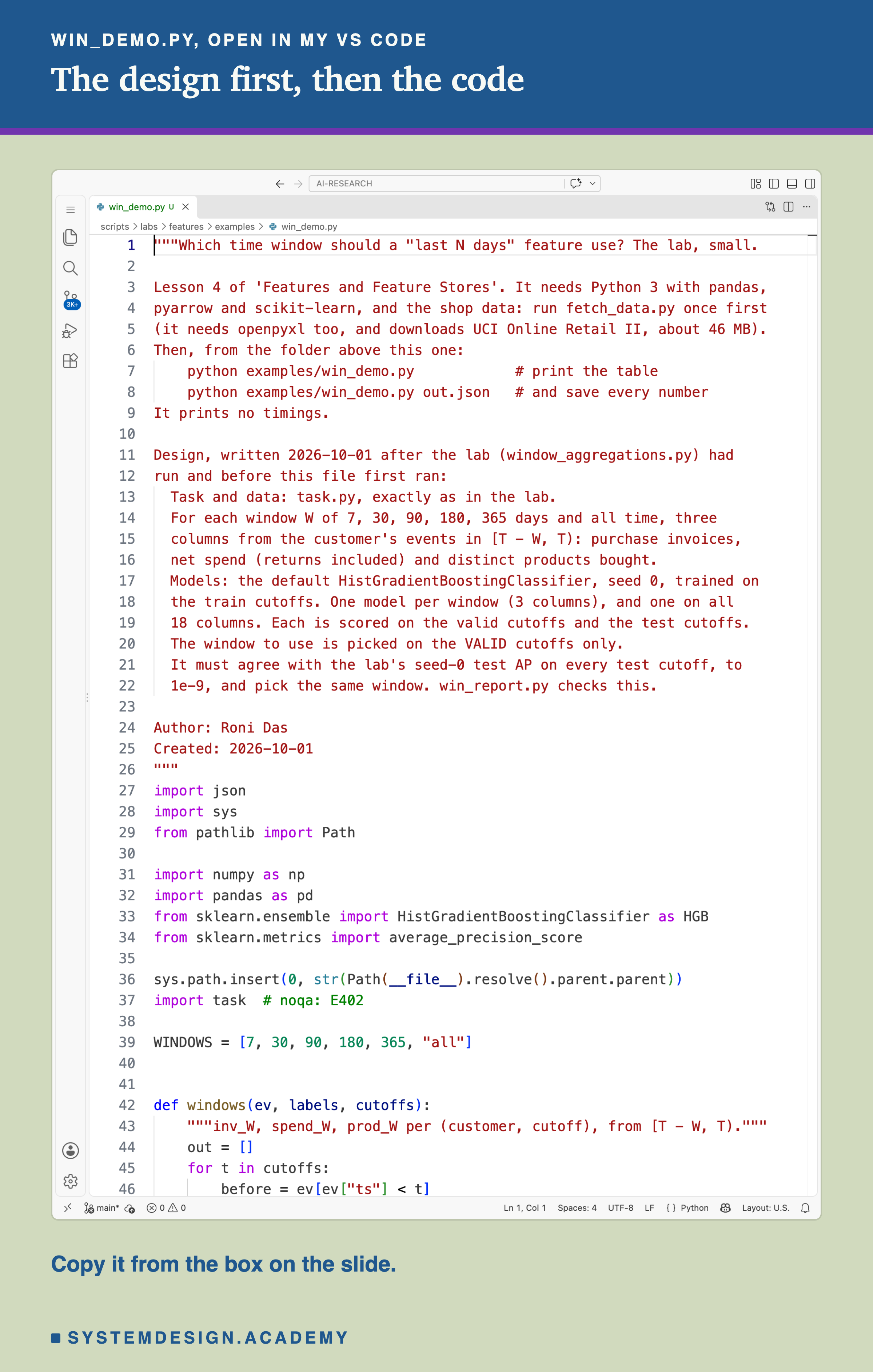
I wrote the demo's design into its docstring after the lab had run and before the demo first ran. It builds the windows with plain boolean filters instead of searchsorted, which is slower but easier to read.
Before you run this lab. You need Python 3 with pandas, pyarrow and scikit-learn: pip install pandas pyarrow scikit-learn openpyxl. First run python fetch_data.py from the scripts/labs/features folder. It downloads the shop data once, about 46 MB, and writes one cleaned file. Then run the demo from the same folder. It needs no GPU. I ran it with scikit-learn 1.9.1 and pandas 3.0.6 on a Mac, where it took under a minute. These libraries run on Windows and Linux too, but I have not checked the numbers there. Give it a file name, python examples/win_demo.py out.json, and it also saves every number. That is how results/win-demo.json was made.
"""Which time window should a "last N days" feature use? The lab, small.

Lesson 4 of 'Features and Feature Stores'. It needs Python 3 with pandas,
pyarrow and scikit-learn, and the shop data: run fetch_data.py once first
(it needs openpyxl too, and downloads UCI Online Retail II, about 46 MB).
Then, from the folder above this one:
    python examples/win_demo.py            # print the table
    python examples/win_demo.py out.json   # and save every number
It prints no timings.

Design, written 2026-10-01 after the lab (window_aggregations.py) had
run and before this file first ran:
  Task and data: task.py, exactly as in the lab.
  For each window W of 7, 30, 90, 180, 365 days and all time, three
  columns from the customer's events in [T - W, T): purchase invoices,
  net spend (returns included) and distinct products bought.
  Models: the default HistGradientBoostingClassifier, seed 0, trained on
  the train cutoffs. One model per window (3 columns), and one on all
  18 columns. Each is scored on the valid cutoffs and the test cutoffs.
  The window to use is picked on the VALID cutoffs only.
  It must agree with the lab's seed-0 test AP on every test cutoff, to
  1e-9, and pick the same window. win_report.py checks this.

Author: Roni Das
Created: 2026-10-01
"""
import json
import sys
from pathlib import Path

import numpy as np
import pandas as pd
from sklearn.ensemble import HistGradientBoostingClassifier as HGB
from sklearn.metrics import average_precision_score

sys.path.insert(0, str(Path(__file__).resolve().parent.parent))
import task  # noqa: E402

WINDOWS = [7, 30, 90, 180, 365, "all"]


def windows(ev, labels, cutoffs):
    """inv_W, spend_W, prod_W per (customer, cutoff), from [T - W, T)."""
    out = []
    for t in cutoffs:
        before = ev[ev["ts"] < t]
        d = pd.DataFrame(index=pd.Index(before["customer_id"].unique(),
                                        name="customer_id"))
        for w in WINDOWS:
            past = before
            if w != "all":
                past = before[before["ts"] >= t - pd.Timedelta(days=w)]
            assert past.empty or past["ts"].max() < t
            buys = past[~past["is_return"]].groupby("customer_id")
            d[f"inv_{w}"] = buys["invoice"].nunique()
            d[f"spend_{w}"] = past.groupby("customer_id")["amount"].sum()
            d[f"prod_{w}"] = buys["stock_code"].nunique()
        d["cutoff"] = t
        out.append(d.fillna(0).reset_index())
    return labels.merge(pd.concat(out), on=["customer_id", "cutoff"])


def mean_ap(model, d, cols):
    p = model.predict_proba(d[cols].to_numpy(float))[:, 1]
    d = d.assign(p=p)
    return d.groupby("cutoff")[["label", "p"]].apply(
        lambda g: average_precision_score(g["label"], g["p"]))


ev = task.load_events()
lab_tr, lab_va, lab_te = task.splits(ev)
tr = windows(ev, lab_tr, task.TRAIN_CUTOFFS)
va = windows(ev, lab_va, task.VALID_CUTOFFS)
te = windows(ev, lab_te, task.TEST_CUTOFFS)
print(f"rows: train {len(tr):,}, valid {len(va):,}, test {len(te):,}")

arms = {f"{w}": [f"{k}_{w}" for k in ("inv", "spend", "prod")]
        for w in WINDOWS}
arms["all 18"] = [c for w in WINDOWS for c in arms[f"{w}"]]
print(f"{'window':8s} {'valid AP':>9s} {'test AP':>8s}")
results = {}
for name, cols in arms.items():
    m = HGB(random_state=0).fit(tr[cols].to_numpy(float), tr["label"])
    v, t = mean_ap(m, va, cols), mean_ap(m, te, cols)
    results[name] = {"valid": float(v.mean()), "test": list(map(float, t))}
    print(f"{name:8s} {v.mean():9.4f} {np.mean(t):8.4f}")

singles = [f"{w}" for w in WINDOWS]
pick = max(singles, key=lambda k: results[k]["valid"])
print(f"picked on the valid months: {pick} days, "
      f"test AP {np.mean(results[pick]['test']):.4f}")
if len(sys.argv) > 1:
    json.dump({"pick": pick, "arms": results}, open(sys.argv[1], "w"),
              indent=1)
Pick a Window Yourself
This box holds the lab's real numbers for all 14 contestants: the valid AP, and the test AP for each of the five test months. It needs nothing but Python, so it runs in your browser. Press Run to see the table, the window picked on the valid months, and the six compared with all windows month by month.
Then change PICK_ON to "test" and run again. You will see what hindsight would pick, and how little it would have gained. Last, change the two names on the line that starts with A, B = to any two names from the table, such as "single_7" and "single_30".
The report script writes this box from the stored lab results, at the full precision the lab stored. It then runs the box with both settings of PICK_ON and checks that it prints the lab's picks and means.
Common Mistakes, and When Each Choice Helps
Copying a window from the last project. "7 days" is a common default. Here 78.7 percent of test rows had no event in the last 30 days. For a 30-day question on that shop, a 7-day window alone barely beat a random guess. Measure your own windows on your own task.
Assuming the longest window is safest. All time lost to 180 days in every test month here. Longer is not always better.
Choosing the window on the test months. It is tempting, because the test months are the numbers you report. Here the honest pick and hindsight were nearly equal, but on another task the gap could be large, and you would never know.
Letting the window touch the cutoff. The window must end strictly before the cutoff. pandas' rolling with a time window like "7D" is a common tool for this. Its default is closed='right', which includes the row at the right end of the window. So if a row sits at the cutoff itself, you want closed='left', which leaves it out. Test a few rows by hand either way.
Many windows that sit close together. 365 days and all time were 0.98 correlated. Pick windows that are far apart.
When several windows help most. This is my guess, not something this lab tested. It is when customers differ a lot in how often they act, so that a short window describes some of them and a long one the rest.
When one window is enough. When the cost of each column matters more than a small gain. Or when your features already include recency and history, and one well-chosen window gets most of the way there.
What This Lab Cannot Tell You
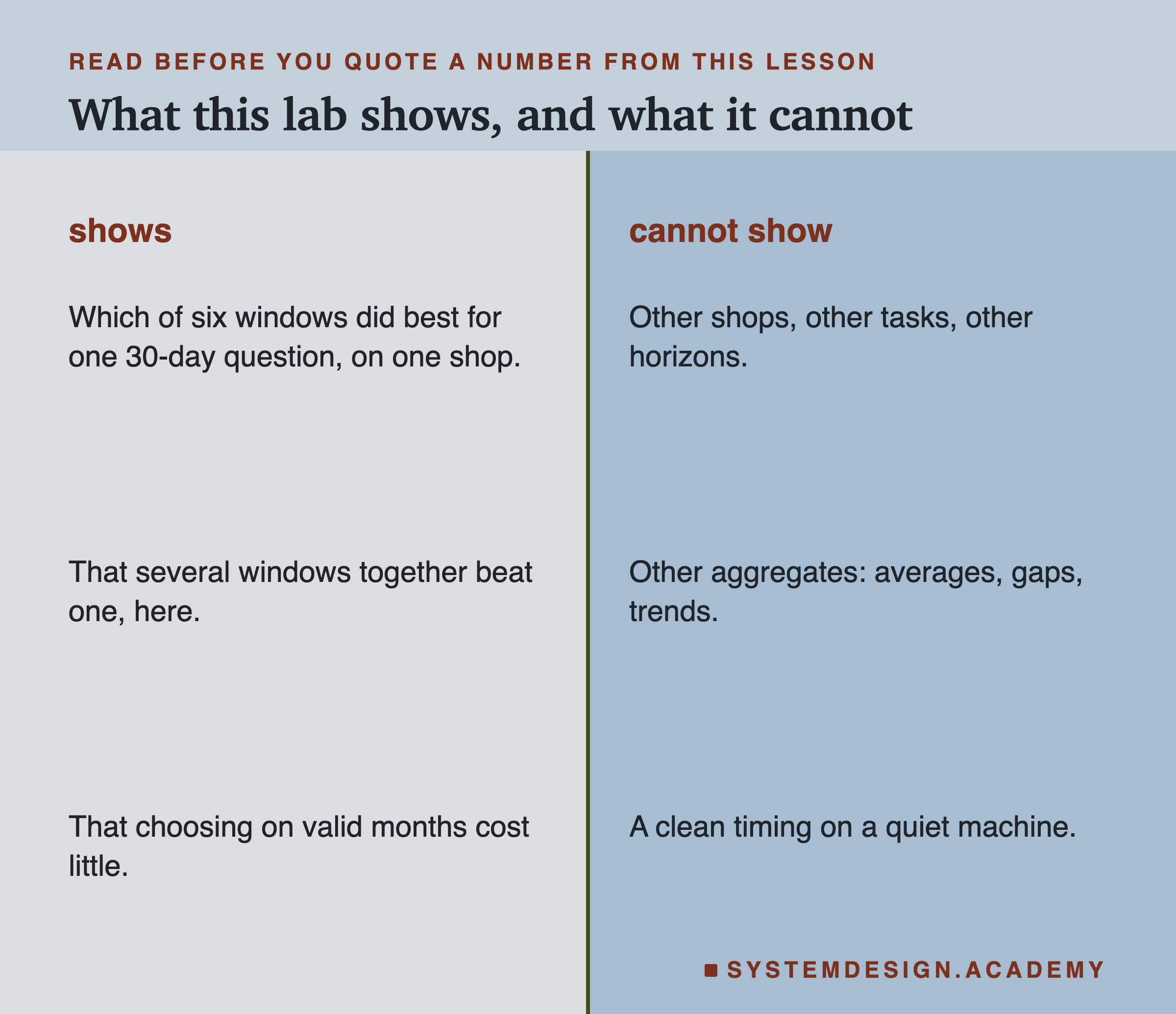
One shop and one 30-day task. My guess is that the best window depends on how often customers act and on how far ahead you predict. A next-day question might favour short windows, and a next-year question long ones. I did not test either.
Three simple aggregates. I counted invoices, summed spend and counted products. Averages, the time between orders, or a trend from one window to the next could behave differently.
Six windows only. I did not try 14, 60 or 120 days. The correlations suggest close neighbours add little, but that is a guess, not a measurement.
One model, default settings. Two of the single-window fits, 365 days and all time, used all 100 trees the default allows without stopping early. A larger limit might lift those two a little. I did not test it.
No clean timing. The cost side has column counts only, for the reason on the cost slide.
What to Do on Monday
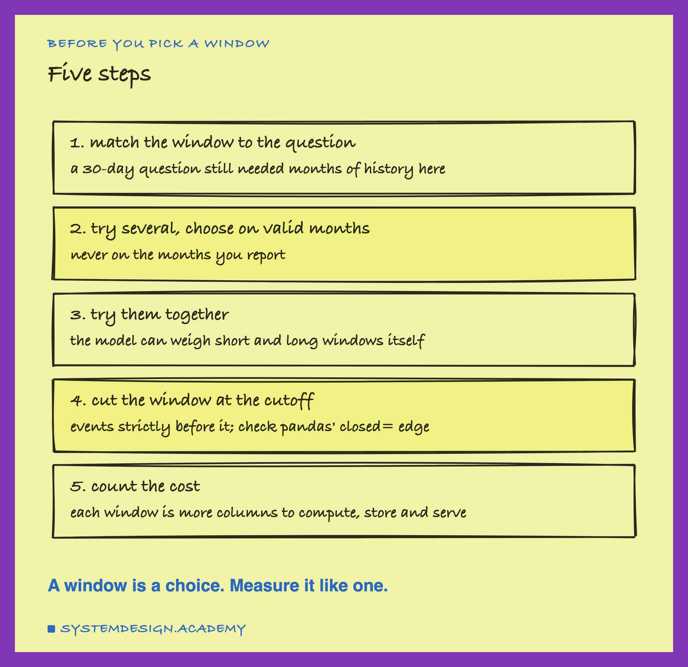
These are the steps I would take the next time someone asks me for "purchases in the last N days".
-
Match the window to the question, and check how many rows each window leaves empty. Here 93.7 percent of test rows had an empty 7-day window.
-
Try several windows, and choose on the valid months. Never choose on the months you report.
-
Try them together. Here all windows beat the best single window in all 5 test months.
-
Cut each window strictly before the cutoff, and assert it in code.
-
Count the cost. Here the best set needed 21 columns against 3 for one window.
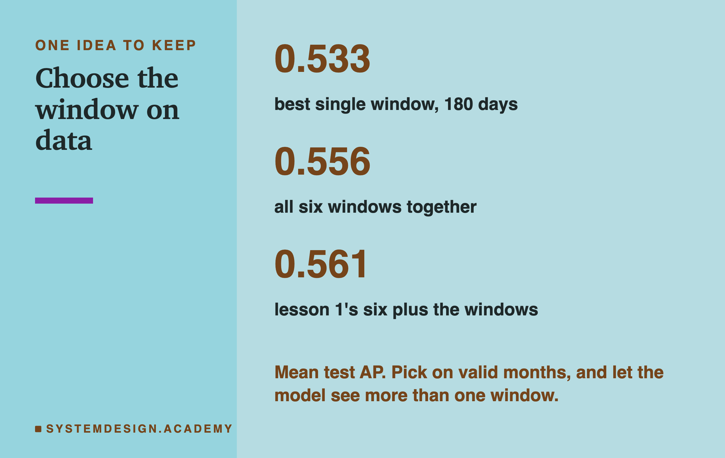
The one idea to keep: a window length is a choice, and it is cheap to measure. On this shop, no single window did as well as several windows together.
Knowledge Check
Knowledge Check
4 questions - Score 80% to pass
Why did the 7-day window alone score an average precision close to a random guess here?
The valid months picked 180 days and the test months would have picked 365 days. What does the lab say about that?
How did all 18 window columns together compare with lesson 1's six made features?
Why did adding a window next to a very similar one add little?