The Person at the Counter Who Knows the Regulars
Let me start with a picture.
Think of the person at the front desk of a busy office, or the counter of a small shop. People come and go all day. After a few months, she can often tell who will be back next week and who will not.
How does she do it? She does not look at the last thing you handed her. She remembers other things about you: how often you come, how long ago you last came, and how much you usually bring.

A machine learning model can only see what you hand it. If you hand it the last receipt, it sees one receipt. If you hand it "comes twice a month, last came four days ago", it sees a regular. Those handed-over facts are called features, and this lesson measures how much they are worth.
Every team argues about one question. When a model is not good enough, should you spend the week on a better model, or on better features? I measured both on the same real data.
The Words You Need First
Please read this slide slowly if any word is new. Every slide after it uses these words.
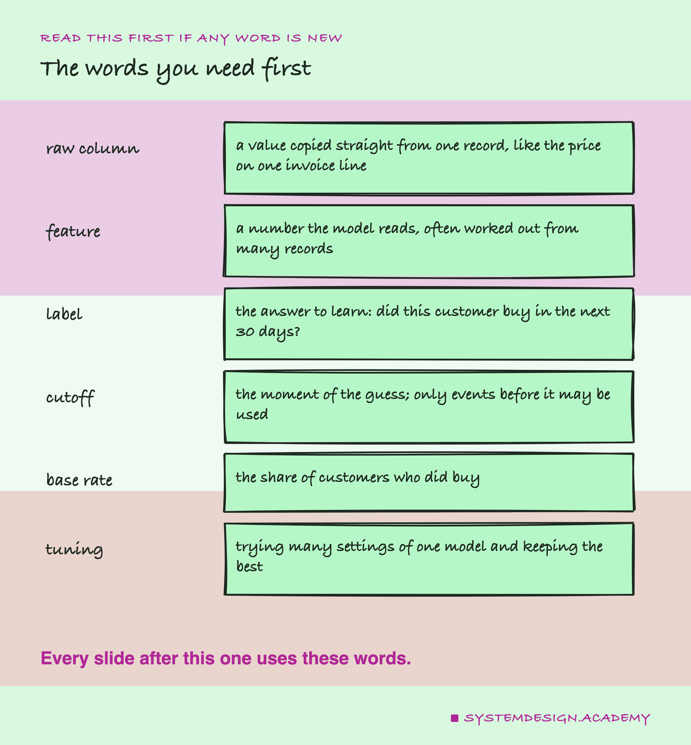
Model. A program that learns a pattern from examples, then uses the pattern to make a guess about new cases.
Raw column. A value copied straight from one record, with no work done on it. The price on one invoice line is a raw column.
Feature. Any number the model reads. In practice the word usually means a number someone worked out, often from many records: "how many orders in the last year" is a feature. I call these made features in this lesson, to keep them apart from raw columns.
Label. The answer the model must learn. Here: did this customer buy again in the 30 days after a given date? Yes is 1, no is 0.
Cutoff. The date of the guess. Everything the model reads must come from before it.
Base rate. The share of customers whose label is 1.
Tuning. Trying many settings of one model, such as how fast it learns or how big its trees grow, and keeping the setting that scores best.
Where This Lesson Starts
This is the first lesson of the chapter on features and feature stores. A is a system that computes features once and hands the same values to model training and to the live app, so the two never disagree.
There is already a survey lesson on feature stores. It explains what a store is, why it keeps an online copy and an offline copy, and what "point-in-time" means, all in words. Please read it if those ideas are new. I will not repeat it here.
This chapter does something different. Each lesson takes one question that the survey answers in words, and measures it on real data. This first lesson asks the most basic question of all. Before you build any system to store features, are features even worth the trouble? If a bigger model could learn the same thing from raw columns, a feature store would be a lot of machinery for nothing.
So I set up a race between a better model and a better feature. Both run on the same rows and the same months, and the raw side sees one line by design. Then I let the data decide.
What a Feature Is, on One Real Customer
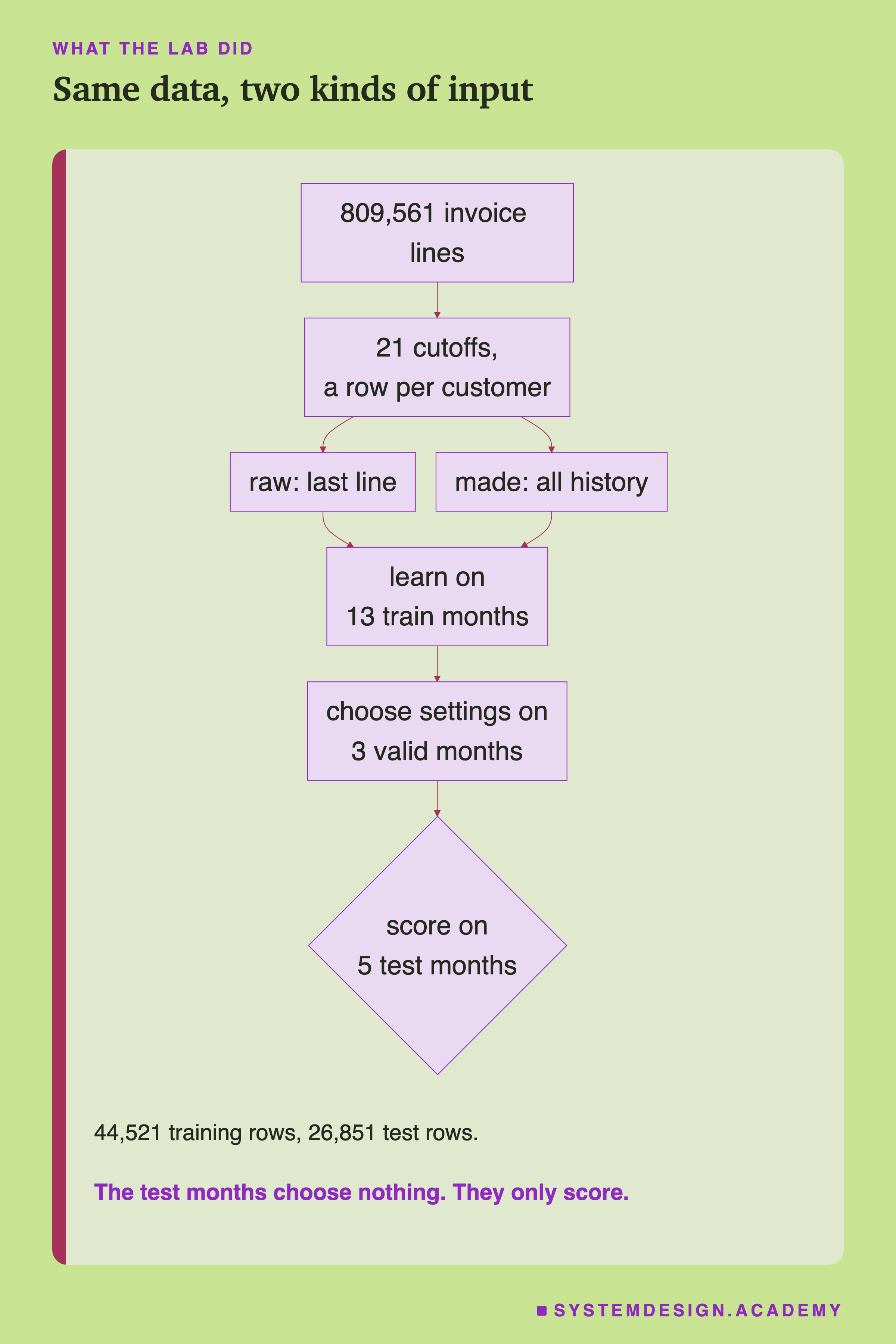
The data is a real shop. It is the Online Retail II dataset on the UCI Machine Learning Repository: every transaction of a UK-based online shop over two years. The shop mainly sells gift items, and many of its customers are wholesalers, people who buy to sell again. The source file has two sheets that overlap for a few days, so 22,523 repeated lines were dropped. After also removing lines with no customer number, there are 809,561 invoice lines from 5,942 customers, from December 2009 to December 2011. Prices are in pounds sterling.
Here is one real customer, number 12349, as the model could see them on 1 July 2011.
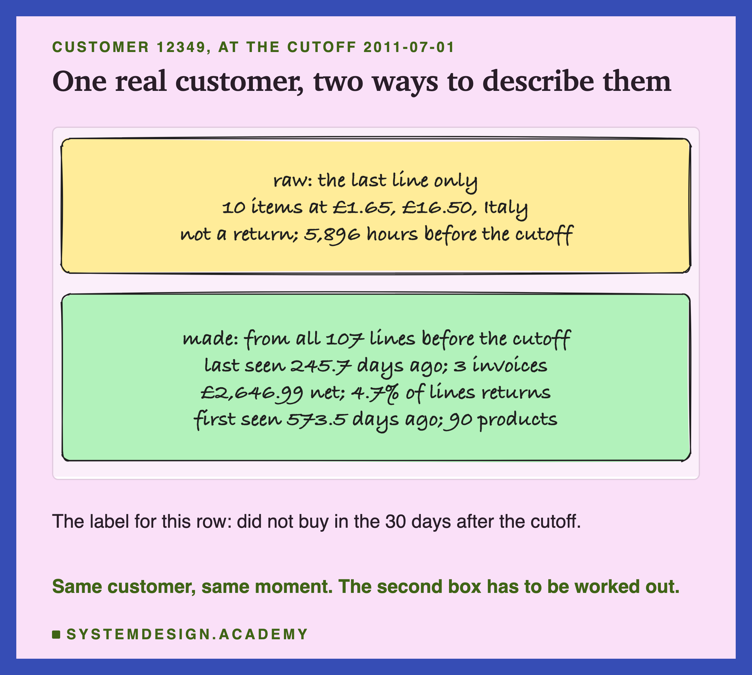
The raw view. The customer's last invoice line before the cutoff: 10 of one item at £1.65, so £16.50, shipped to Italy, not a return, 5,896 hours before the cutoff. That is how one row of the shop's table looks.
The made view. Six numbers, worked out from all 107 of this customer's lines before the cutoff. They last bought 245.7 days ago. They placed 3 orders in all. They spent £2,646.99 after returns. 4.7% of their lines were returns. They first appeared 573.5 days before the cutoff. They bought 90 different products.
Both views describe the same person at the same moment. Neither contains anything from after the cutoff. The made view simply did some counting first. This customer, as it happens, did not buy in the next 30 days.
The Six Made Features, in Plain Words
I did not invent these six. Marketers know the first three as RFM, short for recency, frequency and monetary value, a method used in direct marketing to judge customers. The other three are just as simple.
-
Recency. Days from the customer's last event to the cutoff. Someone who bought last week is more likely to buy again than someone who last bought a year ago.
-
Frequency. How many separate orders they placed. Returns do not count as orders.
-
Money. Their net spend: the total of all their lines, with returns taken away, because the shop records a return as a negative amount.
-
Return share. Return lines divided by all lines.
-
Tenure. Days since the customer was first seen in this data, which starts in December 2009. A long tenure with few orders tells a different story from a short one.
-
Products. How many different products they bought.
One fact surprised me when I wrote the code, so I checked it in the lab. The raw view's "hours since the last line" is exactly the made view's recency times 24, for every row. The last line always sits on the last event. So both views already carry recency. The race really measures what the other columns add.
The Question the Model Must Answer
Every lesson in this chapter shares one task. On the first day of a month, for every customer seen before that day, guess: will they buy again in the next 30 days?
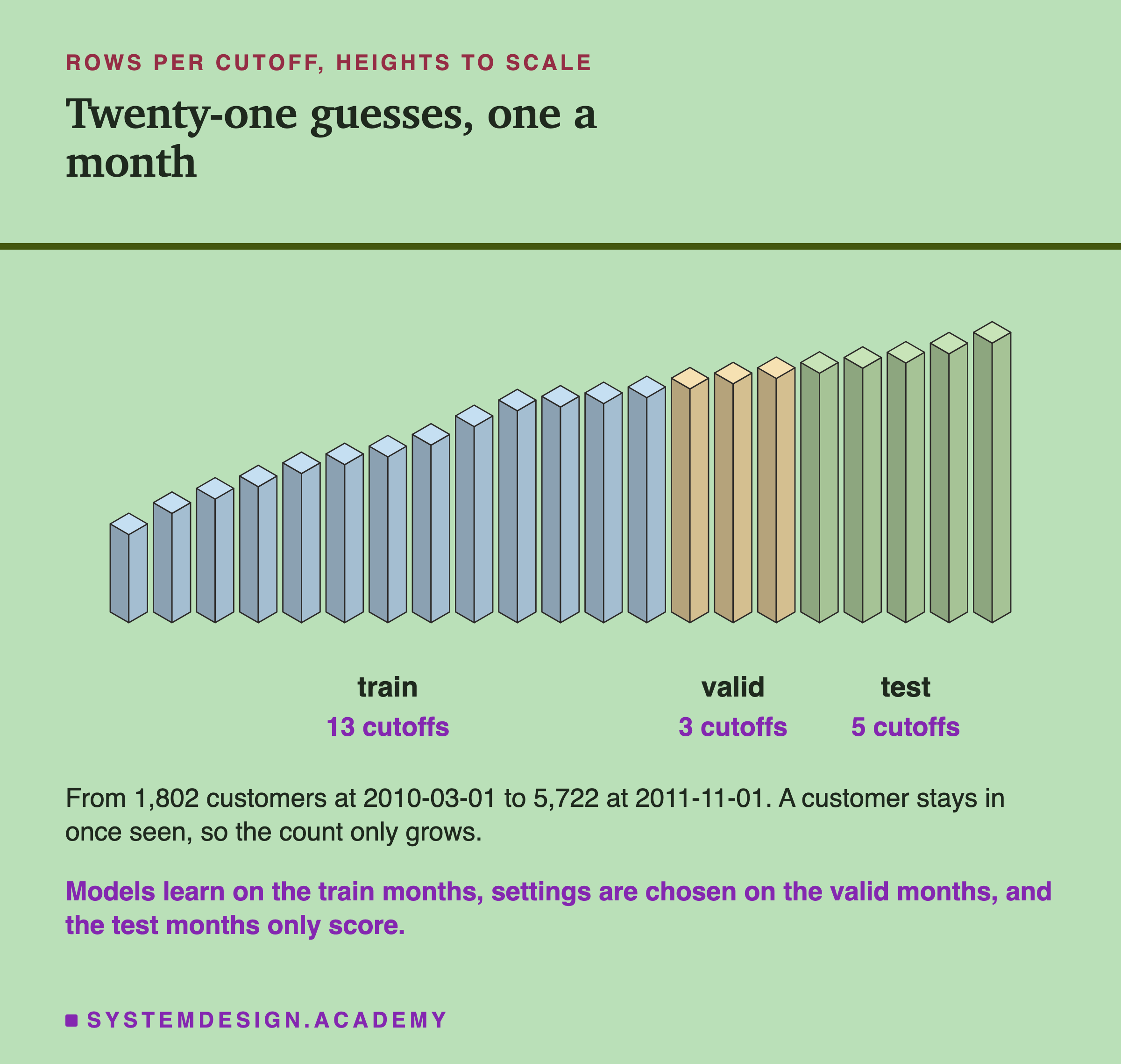
Each first of the month is a cutoff, and each cutoff gives one row per customer. The cutoffs are split by time into three groups, and the split matters a great deal.
Train months. March 2010 to March 2011, 13 cutoffs and 44,521 rows. The models learn from these.
Valid months. April to June 2011, 3 cutoffs and 14,673 rows. When I need to choose something, such as the best of many settings, I choose it here.
Test months. July to November 2011, 5 cutoffs and 26,851 rows. These only score. Nothing is ever chosen by looking at them, so their score is a fair preview of new months.
The share of customers who bought again, the base rate, moved from month to month. Over the five test months it was as low as 0.156 in August 2011 and as high as 0.257 in November 2011. Averaged over those five months it was 0.196: about one customer in five. Across all 21 cutoffs it ran from 0.145 to 0.340.
Only the Past, Checked in Code
There is one rule that every feature in this chapter obeys. A feature may only use events from strictly before the cutoff. The label uses the 30 days from the cutoff onward. Nothing may cross that line.
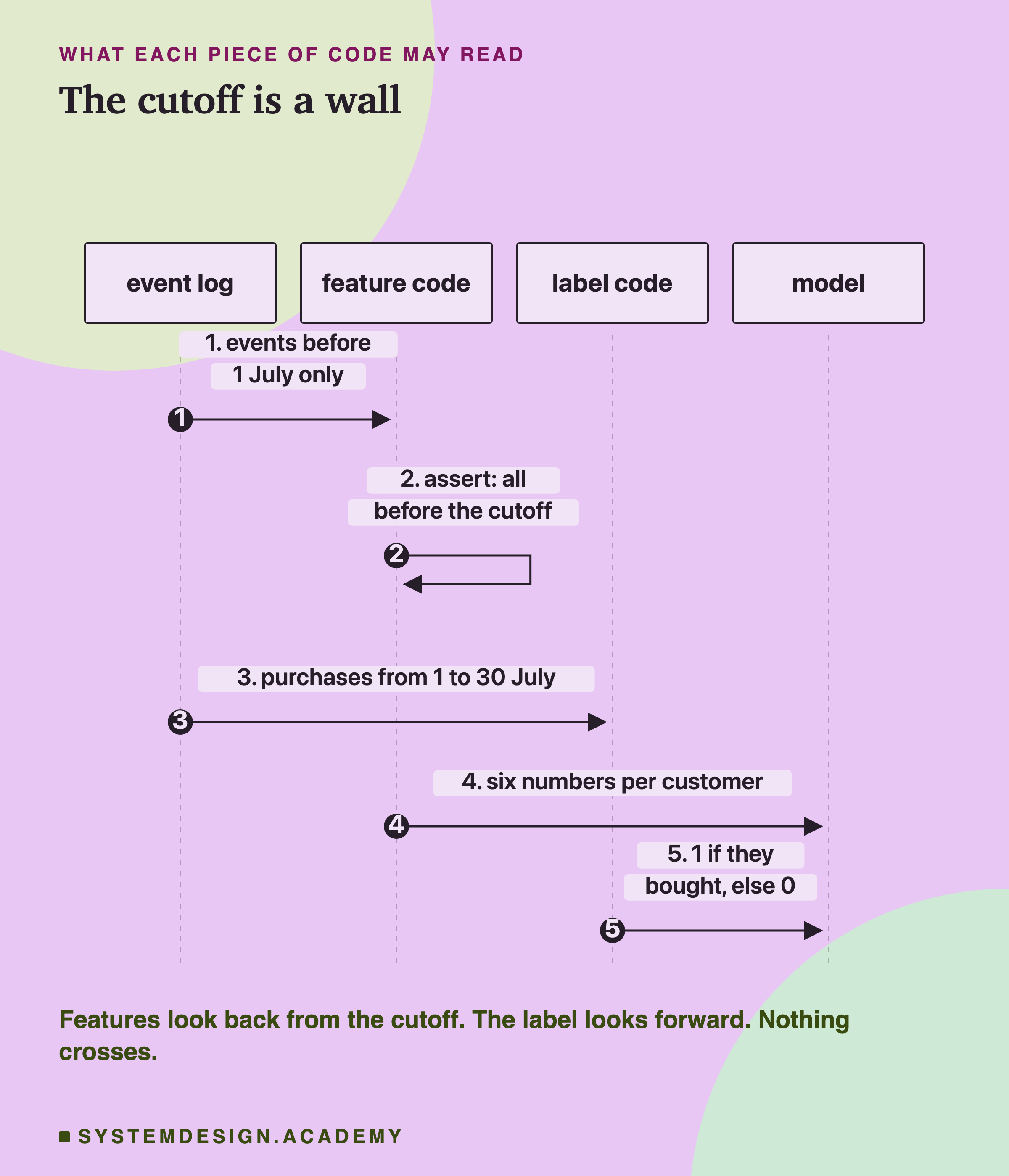
Why be so strict? If one future event slips into a feature, the model gets a peek at the answer. Its score in the lab then looks better than anything it can do for real, where the future is not yet written. The survey lesson calls this label leakage, or leaking the future into the past, and lesson 2 of this chapter measures how much it inflates a score.
So I did not only intend to respect the rule. The lab checks it. For each cutoff it takes only the rows before the cutoff, then asserts four things. The newest event used is older than the cutoff. Every customer's last event is older than the cutoff. Every "hours since" is above zero. And each customer's last line sits on their last event. If any check fails, the lab stops with an error instead of printing a number.
How I Score a Guess: Average Precision and ROC-AUC
The model does not answer yes or no. It gives each customer a score, and a higher score means "more likely to buy". What the shop would do with that is sort the customers by score and call, or email, the ones at the top. So I score the sorted list, not single answers.
Average precision (AP). Walk down the sorted list from the top. Each time you reach a customer who really did buy, look at the share of buyers among everyone you have passed so far. That share is called precision. AP is the average of those precision values, one for each real buyer. If every buyer sits at the very top, AP is 1. If the list is in random order, AP lands near the base rate, here about 0.196. So the base rate is the floor to beat, not zero.
ROC-AUC. Pick one random buyer and one random non-buyer. ROC-AUC is the chance that the model gave the buyer the higher score. 1 is perfect. 0.5 is a coin flip.
Why both? They answer slightly different questions. ROC-AUC weighs the whole list evenly. AP cares most about the top of the list, which is the part a shop actually uses, and it moves more when buyers are rare. I report AP as the main score and ROC-AUC beside it, for each of the five test months and as their plain average.
How the Lab Was Built
I wrote the design of the lab into its docstring on 1 October 2026, before the first run. At that point I had looked at the shape of the data and nothing else. No model had been trained on this task.
The main model is called gradient boosting. It builds many small decision trees, one after another. A decision tree is a chain of yes-or-no questions about the inputs, like "is recency more than 60 days?". Each new tree tries to fix the mistakes of the trees before it. I used scikit-learn's HistGradientBoostingClassifier with its default settings and a fixed seed of 0. A seed is a number that fixes the random choices inside training, so a run can be repeated exactly.
The design also wrote down my guess before the run, so the guess could be wrong in public. I expected made features to beat raw columns, tuning to beat the default model, and made features to beat tuning.
The next slide lists every contestant. They all learn from the same 44,521 training rows and are scored on the same 26,851 test rows.
Seven Ways to Rank Customers
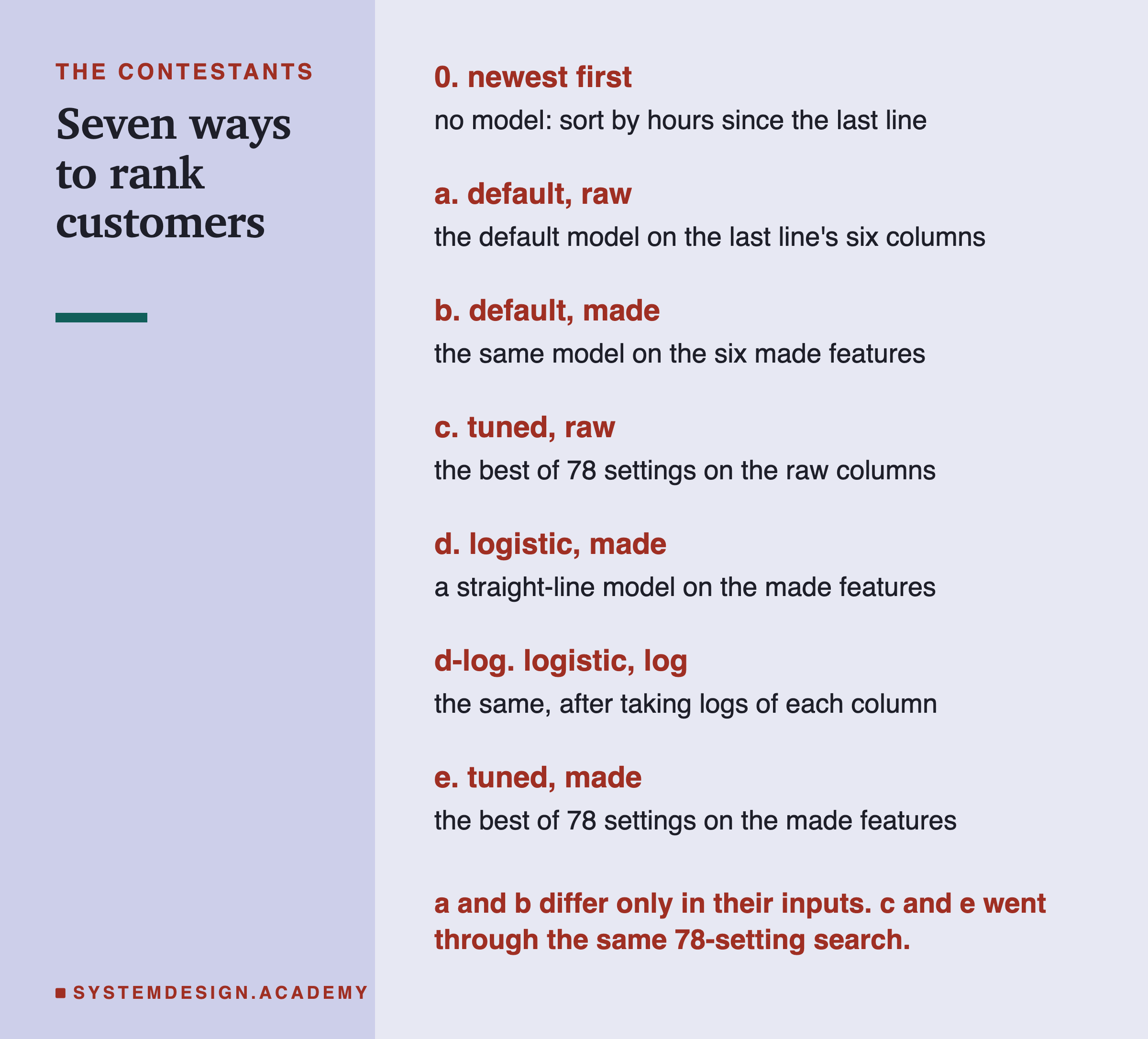
0. Newest first. No model at all: sort customers by how recently they last appeared. Any model must beat this to be worth its cost.
a. The default model on raw columns. The last line's quantity, price, amount, country, return flag and hours since.
b. The same default model on the six made features. Only the input changes.
c. A tuned model on raw columns. I tried 78 settings. 72 were gradient boosting, changing how fast it learns, how big its trees grow, how many rows a leaf needs and how much it is held back. A leaf is the end of a tree's chain of questions, where it gives its answer. The other 6 were a random forest, a different family that averages many independent trees. Each was trained on the train months and scored on the valid months. The best one was kept.
d. Logistic regression on the made features. A much simpler model. It gives each feature a weight and adds them up, so it can only draw a straight dividing line.
d-log. The same, after taking the logarithm of each feature. A logarithm squeezes large numbers together: in base 10, 10 becomes 1, 100 becomes 2 and 1,000 becomes 3. I added it to the design before the run, because money and frequency run from very small to very large numbers.
e. A tuned model on the made features, chosen the same way as c. I added it before the run so that "do the two gains add up?" was a planned question.
The Answer: Better Features Won, by a Wide Margin
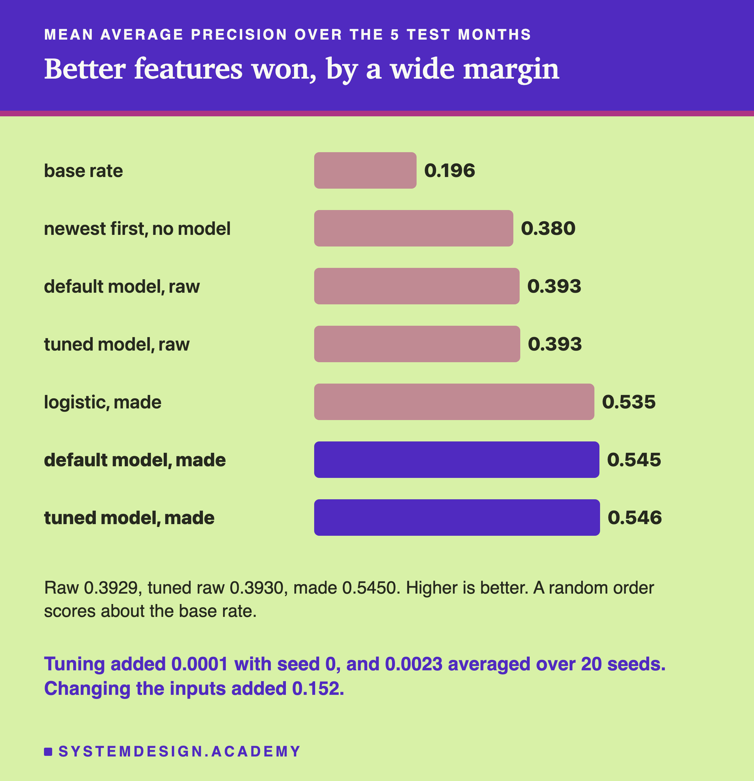
Here is every contestant, from the lowest mean average precision to the highest. ROC-AUC sits beside it, and each number is the plain average over the five test months.
| contestant | inputs | mean AP | mean ROC-AUC |
|---|---|---|---|
| 0. newest first | hours since | 0.380 | 0.757 |
| a. default model | raw | 0.393 | 0.757 |
| c. tuned model | raw | 0.393 | 0.759 |
| d-log. logistic, logs | made | 0.527 | 0.792 |
| d. logistic | made |
The Lab's Report, Running
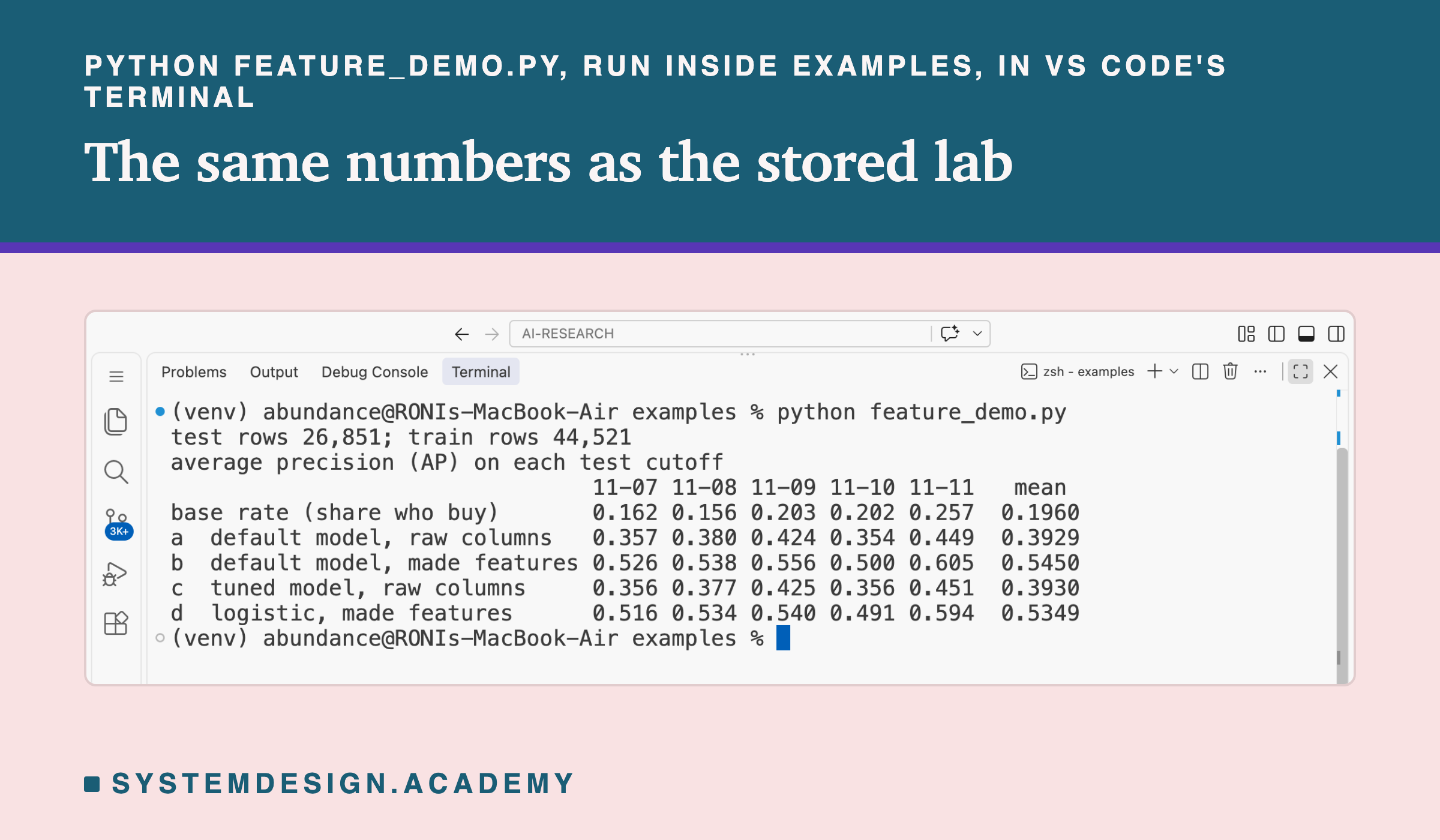
This is a real recording of the lab's report script, printed on the laptop where the lab ran. The report does not train anything. It reads the stored results and recomputes every number in this lesson from them.
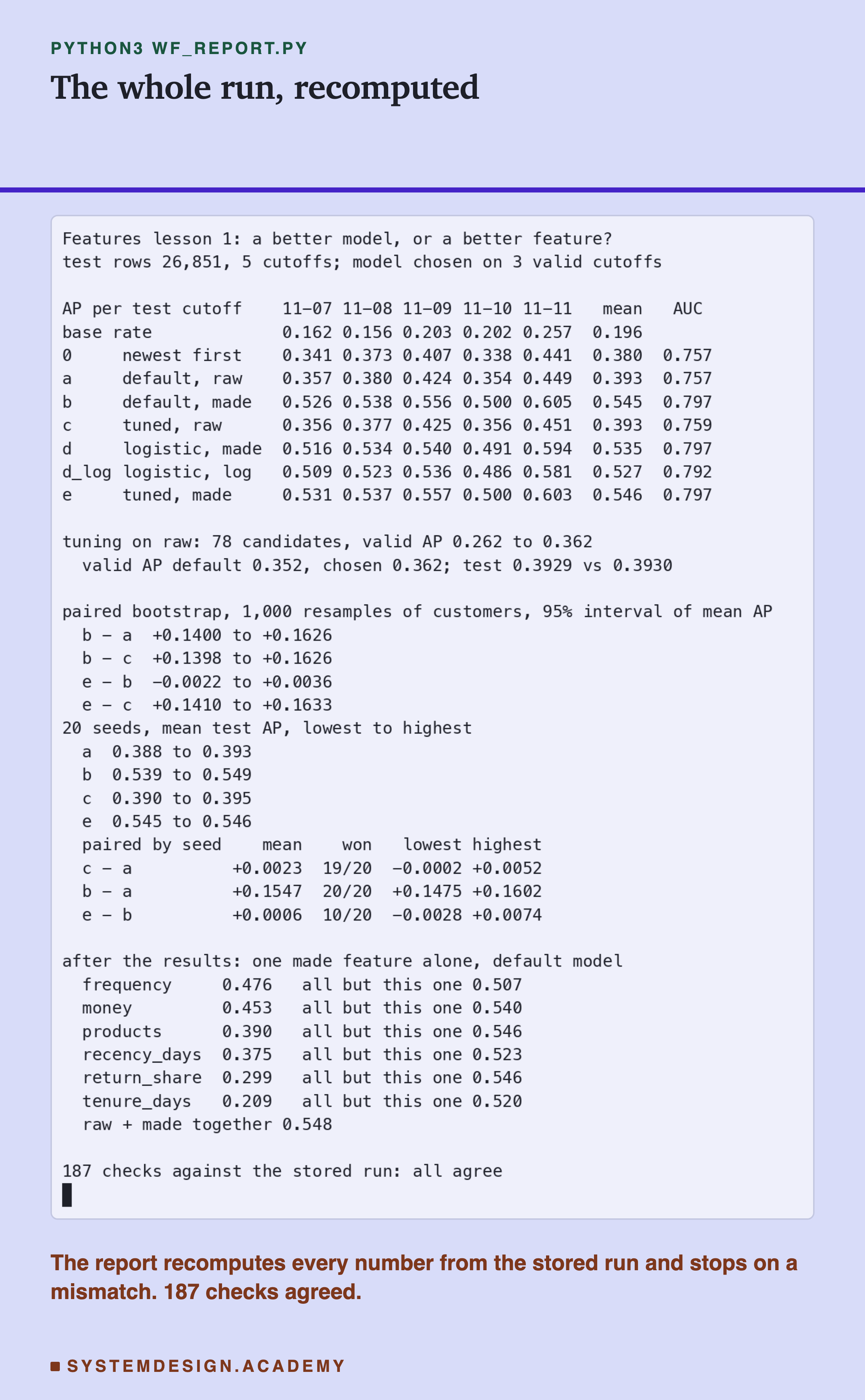
In the recording, each column headed with a date like "11-07" is one test month, July 2011. "made" means the six made features. "valid AP" is the score on the valid months, which is where tuning made its choice.
The report checks each mean against the per-month numbers it came from, and each bootstrap interval against the 1,000 stored resamples. It also checks that the student demo, later in this lesson, printed the same numbers as the lab. Last, it checks that every number this lesson quotes appears in the lesson text. If anything disagrees, it stops and exits with an error.
Every Month, Not Only on Average
An average over five months could hide one wild month. So here is each month on its own.
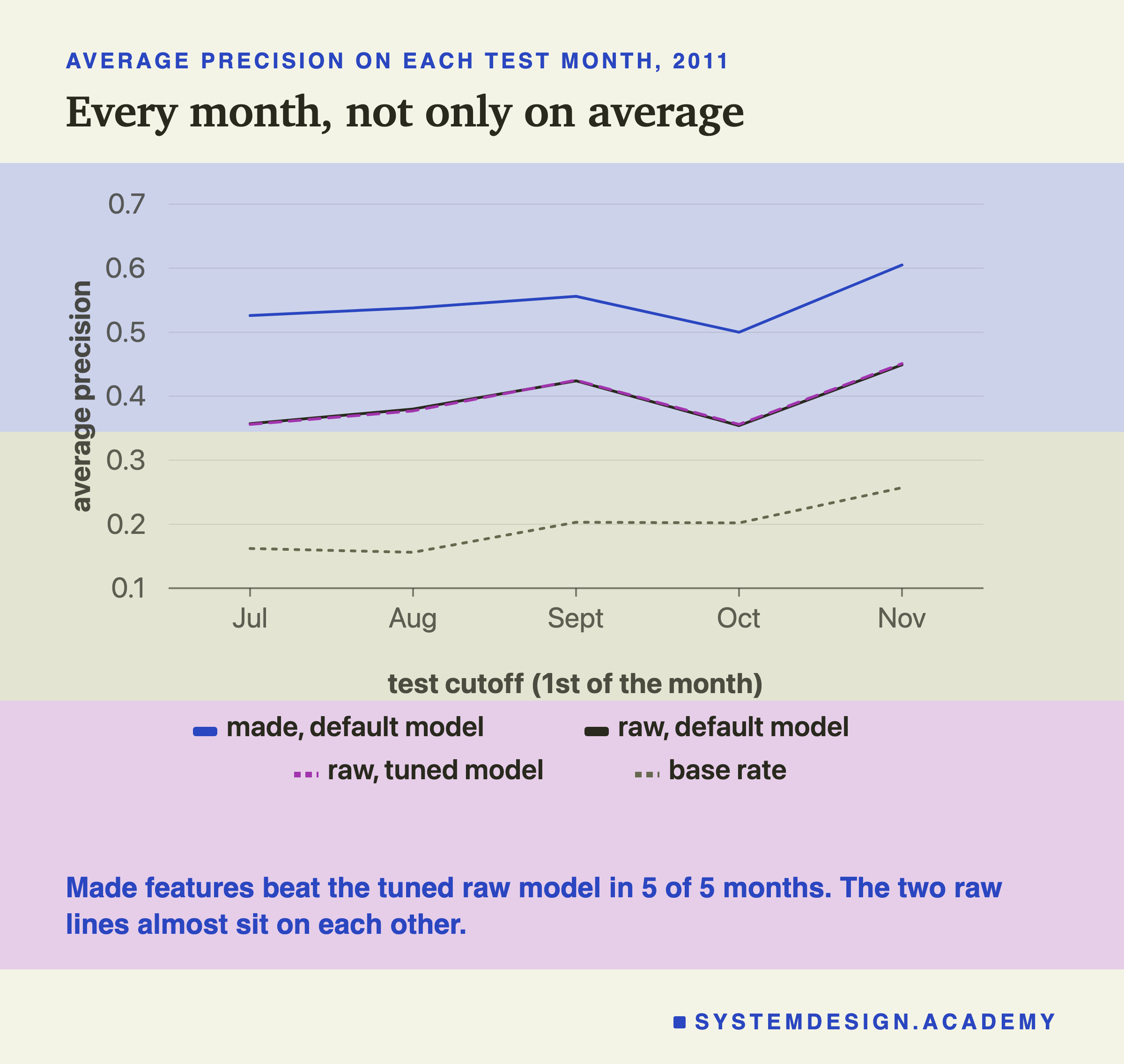
The made features beat the tuned raw model in 5 of 5 months. The gap never closed: the made line sits above the raw lines all the way across.
The tuned and default raw models took turns. With seed 0, the tuned one was higher in 3 of the 5 months and lower in the other 2. Month by month, the two were close to level. The 20-seed check two slides on shows the tuned one was slightly, but steadily, ahead.
Notice also that every line rises and falls together. October was a hard month for every contestant and November an easy one. Part of the reason is the base rate: in November 0.257 of customers bought again, against 0.202 in October. A month with more buyers is easier to score well on, so the AP of different months should not be compared with each other. Only contestants within the same month should be compared.
The Gains, Worked by Hand
You can check the headline with a pencil, from the four-place means the lab stored.
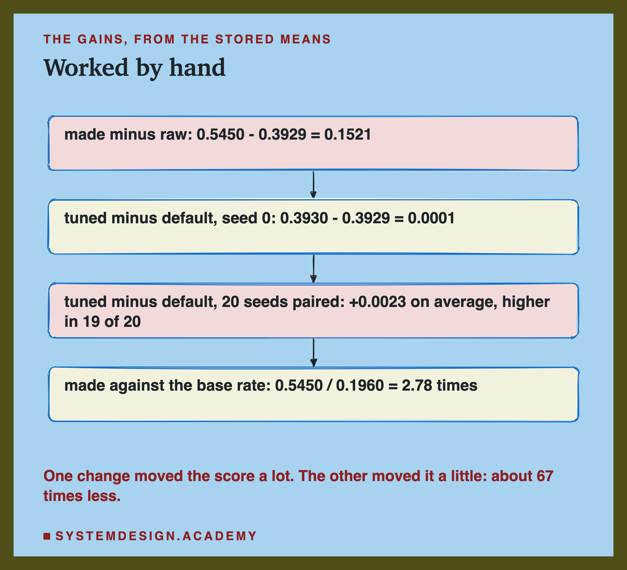
The feature gain. 0.5450 minus 0.3929 is 0.1521. Rounded to three places, that is the 0.152 on the headline.
The tuning gain. 0.3930 minus 0.3929 is 0.0001. That is with seed 0. Over 20 seeds, paired seed by seed, the tuned model averaged 0.0023 more than the default. Both are small next to the 0.152 from the features.
Against the floor. A random order scores about the base rate, 0.1960. The made features scored 0.5450, about 2.78 times that. The raw model scored 0.3929, about 2.0 times. So the made features did not just add a bit on top. They moved the model much further from guessing.
The program that draws these figures also checks each difference above. Worked from the rounded numbers, it must match the unrounded difference, rounded once. If those ever disagreed, a number would have been rounded twice, and it would stop.
What 78 Settings Bought
Why did tuning do so little? The tuning itself shows it.
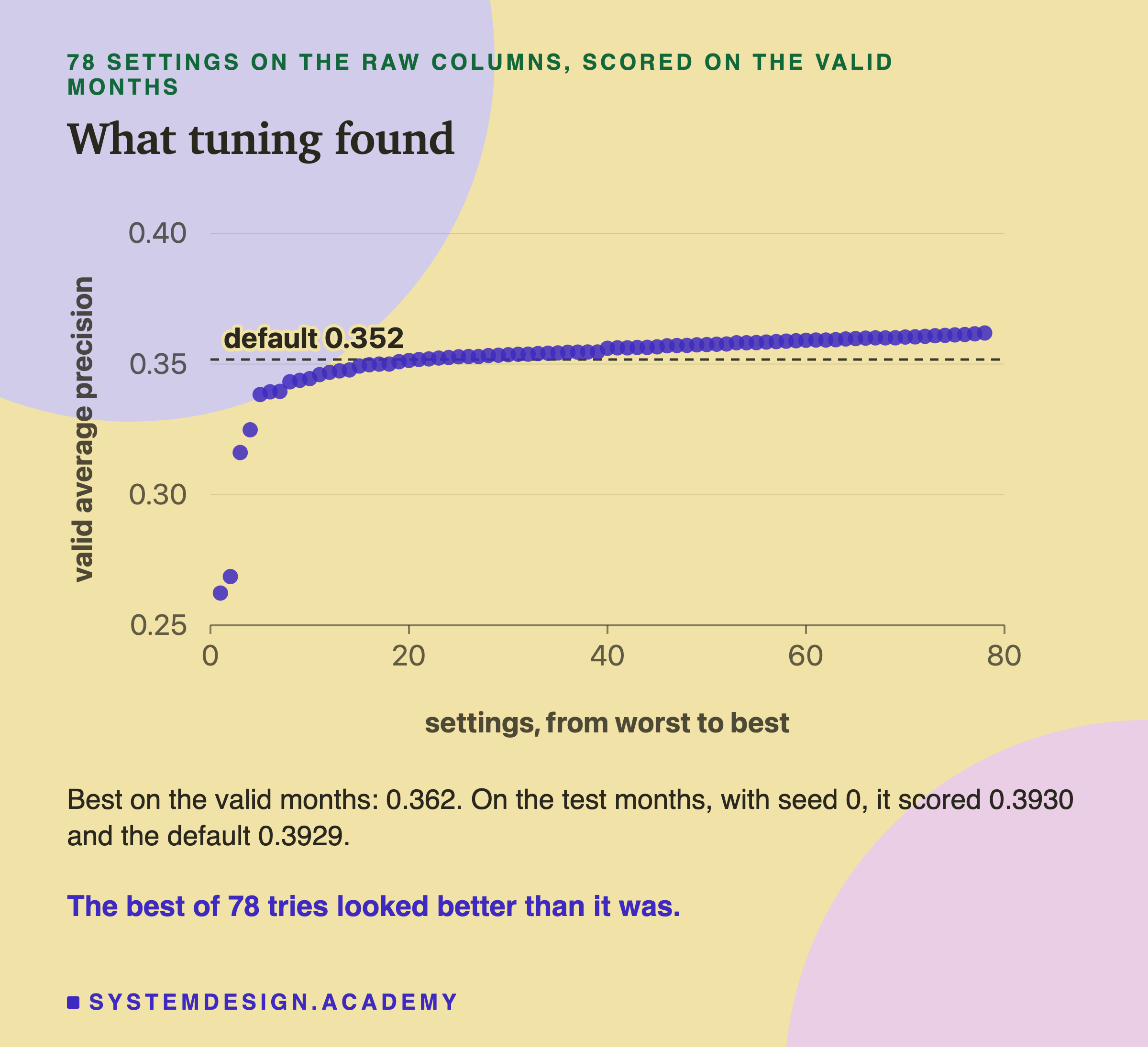
On the valid months the 78 settings scored from 0.262 to 0.362. The four worst were random forests whose leaves could hold as few as 1 or 5 rows. One possible reason, which I did not test: trees with such tiny leaves fit the training rows too closely. Most of the settings crowded into a flat line just above the default model's 0.352.
The best was 0.362: a slow learning rate, small trees of 7 leaves, and at least 400 rows in each leaf. All three of those sit at the edge of the grid I searched: the slowest rate, the smallest trees and the biggest leaves. A wider search might find a little more.
So on the valid months, tuning seemed to buy 0.010. On the test months most of that gain went away: 0.3930 against 0.3929 with seed 0, and 0.0023 on average over 20 seeds.
This is a well-known trap. When you try 78 settings and keep the best, the best one is partly the best and partly the luckiest on those three valid months. Its valid score is too high, and new months bring it back down. The valid months did their job: they stopped me from fooling myself on the test months.
There is a deeper reason too. Tuning changes how a model learns from its inputs. It cannot add information the inputs do not hold. The raw last line simply does not say how often a customer comes back.
How Sure Can I Be?
One run on one split could be luck. I checked two kinds of luck.
Luck in training. By default, this model holds back 10% of the training rows, picked at random, to decide when to stop adding trees. This is called early stopping, and scikit-learn turns it on by itself when there are more than 10,000 rows. I did not choose that. It is a library default, which I looked up and wrote into the design before the run. It means the seed changes the result a little. The default raw model stopped after 44 trees of the 100 it was allowed, and the tuned one after 236 of 500. So I retrained four contestants with 20 different seeds.
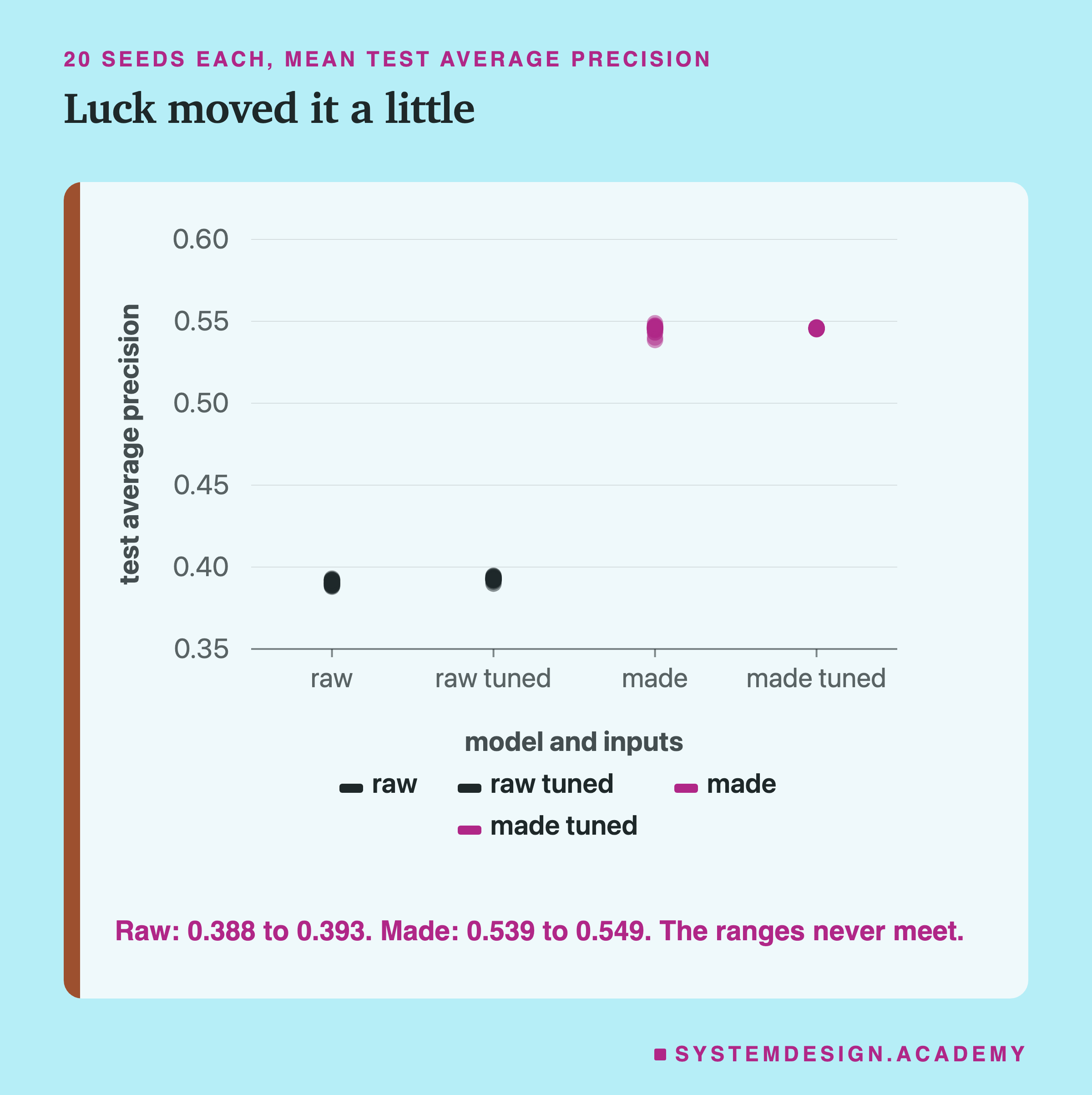
Over 20 seeds, the default raw model ranged from 0.388 to 0.393, the tuned raw model from 0.390 to 0.395, and the made-feature model from 0.539 to 0.549. The raw and made ranges never come close.
The seeds also give a fairer view of tuning, because I can pair them: seed 1 tuned against seed 1 default, and so on. The tuned model was higher in 19 of 20 pairs, by 0.0023 on average, from -0.0002 to 0.0052. So the tuning gain was real but small. The made features beat the default raw model in every pair, by 0.155 on average.
Luck in which customers were tested. A bootstrap asks: if the test months had held a slightly different set of customers, how much would the gap move? It draws the customers again at random, with repeats allowed, 1,000 times, and works out the gap each time. The middle 95% of those gaps is called a 95% interval. For made features against the tuned raw model, it ran from 0.140 to 0.163. Every one of the 1,000 draws favoured the made features.
Do the Two Gains Add Up?
Contestant e was planned to answer this: what happens when you tune the model on the made features too?
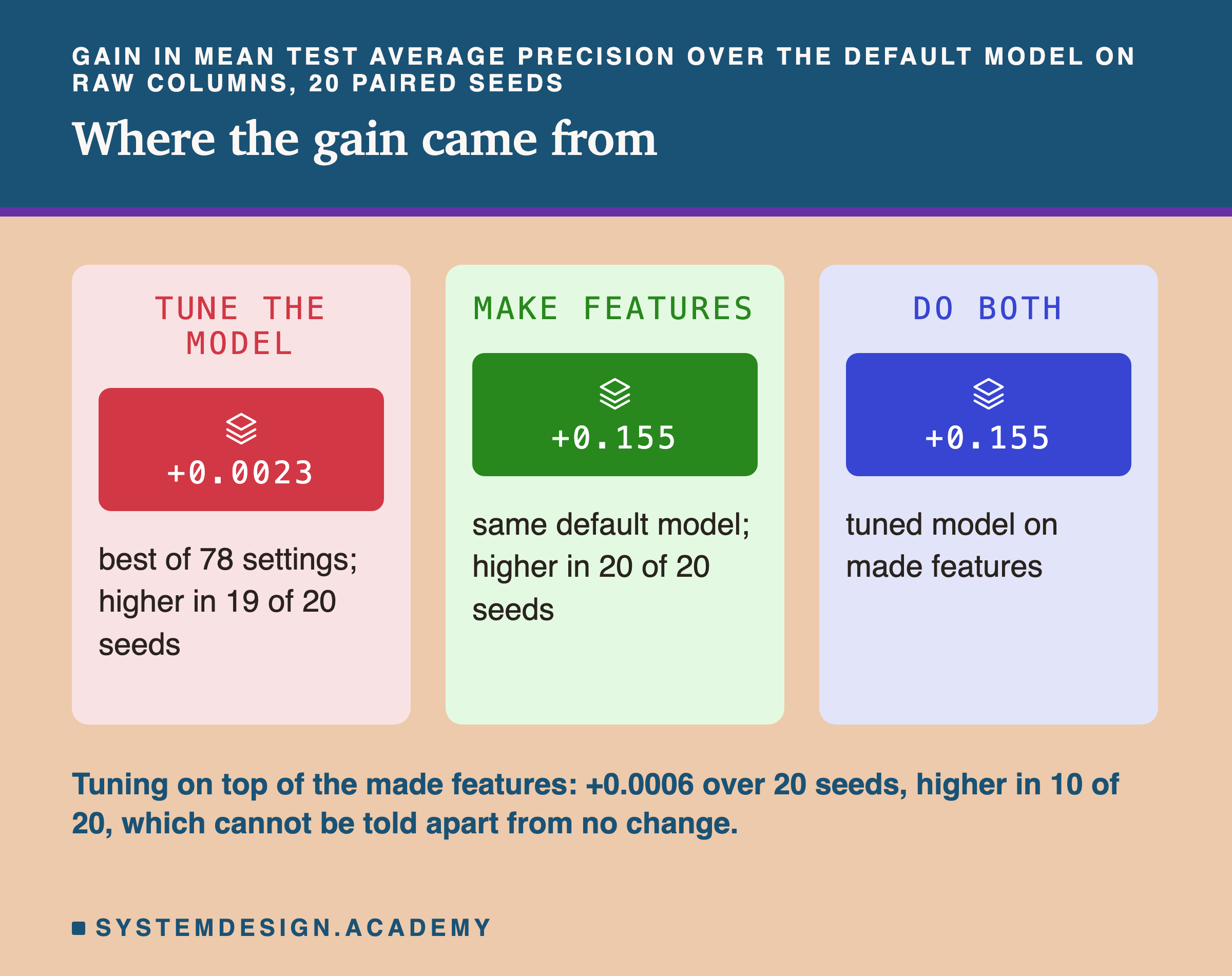
The tuned model on made features scored 0.5457, against 0.5450 for the default model on the same features. The tuning picked a random forest this time, with at least 20 rows in each leaf, which is also the edge of its grid.
Is that 0.0007 real? The bootstrap interval for the gap ran from -0.0022 to 0.0036. It includes zero, so this gap cannot be told apart from luck. Month by month, the tuned model won 2 of 5. Over 20 paired seeds it won 10 of 20, by 0.0006 on average. So, on this data, tuning did not add anything I could detect on top of the features either.
I want to be careful with what this means. It does not prove tuning is useless. Tuning was useful insurance here: it confirmed that the default settings were already close to the best of the 78 alternatives. What it shows is narrower. On this task, the first and largest step was choosing what to hand the model, and no amount of setting-changing made up for handing it the wrong thing.
Which Feature Did the Work? Asked After the Results
The main results made me curious about something the design had not asked. Which of the six made features carried the gain? I wrote this second question into the lab's docstring after seeing the main results, and before it ran. Everything on this slide comes from that later run, so please read it as a follow-up, not as part of the original plan.
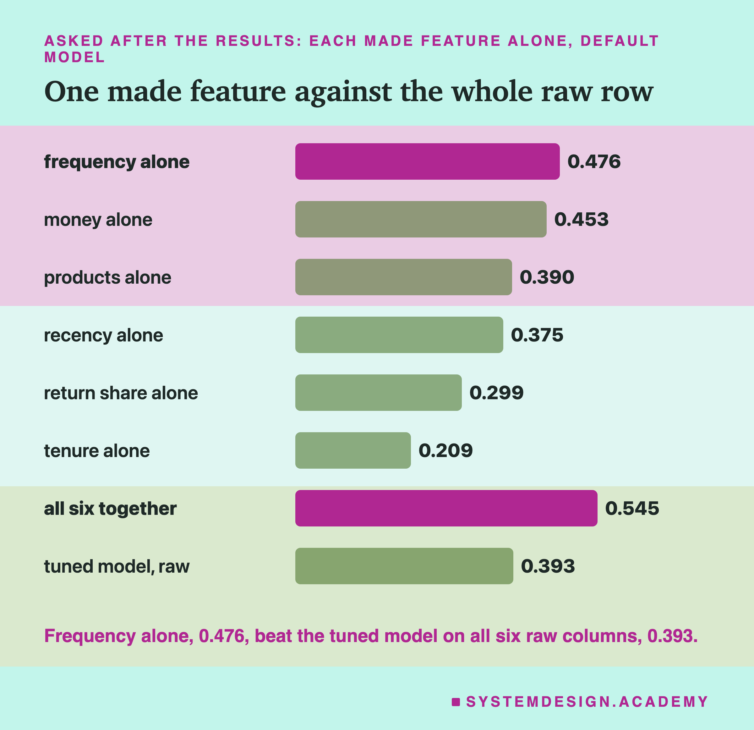
I trained the same default model on each made feature alone, then on all six with one left out.
Frequency, the number of orders, did the most. On its own it scored 0.476, already well above the tuned model with all six raw columns, 0.393. Money alone scored 0.453. Recency alone scored 0.375, close to sorting by recency with no model.
Leaving frequency out of the six dropped the score from 0.545 to 0.507, the biggest drop of any feature. Leaving out return share or products barely moved it, by less than the seed wobble, so those two cannot be told apart from adding nothing.
Last, I gave the model the raw columns and the made features together. It scored 0.548, about the same as the made features alone. Once the history was there, the last line added nothing I could detect. I ran each of these once, with one seed, so treat the small differences between them as rough.
A Simple Model on Good Features
One result deserves its own slide. Logistic regression is one of the simplest models in common use. It gives each input a weight, adds them up, and turns the sum into a chance. It cannot ask "if this, then that" the way trees can.
On the made features it scored 0.535 AP and 0.797 ROC-AUC. On ROC-AUC it tied the gradient boosting model, which scored 0.797 too. On AP it was 0.010 behind. And it was 0.142 ahead of the best tuned model on raw columns.
Because it is so simple, you can read what it learned. I rescaled every feature to the same spread first, so the weights can be compared. The biggest weight went to frequency, 0.91. The next was recency, -0.47: the minus sign means "the longer since they last came, the less likely they come again". Those are the same two facts the person at the front desk remembers.
One more honest note. I planned d-log, which takes logs of each feature first. I expected it to help a straight-line model with money that runs from a few pounds to many thousands. It did not help. It scored 0.527, a little below plain d. My reason for adding it was sensible, and it was still wrong here.
The Lab's Code, Piece by Piece
The lab is one Python file, scripts/labs/features/what_a_feature_is.py. It uses the shared file task.py, which every lesson in this chapter uses, for the data, the cutoffs and the labels. It is worth knowing its main parts before you run anything.
Building both views. The function build_tables runs once per cutoff. It finds where the cutoff falls in the time-sorted events with searchsorted, and keeps only the rows before it. From those rows, groupby("customer_id").tail(1) takes each customer's last line, which gives the raw view. Grouped sums, counts and minimums give the made view. The checks for the cutoff rule sit right there, so a mistake fails loudly at the place it happens.
Joining to the labels. The function joined merges the features onto the label table with validate="one_to_one". That option makes pandas stop with an error if any customer appears twice, which would quietly double-count them.
The country column. Gradient boosting can treat a column as a set of names rather than numbers. scikit-learn calls this a native categorical column: native because the model handles the names itself, with no extra step. I gave country that treatment. Countries are coded from the training months only. A country first seen later becomes "missing" instead of borrowing a code. 5 test rows had such a country.
Tuning. The function tune trains each of the 78 settings on the train months, scores it on the valid months, and keeps the best. The test months are not touched until the very end.
The bootstrap. The function redraws customers within each test month, and uses the same redraw for every contestant. It stores all 1,000 gaps, so the report can check the interval later.
Try It Yourself
The full lab takes several minutes, mostly for the tuning. I wrote a small demo that rebuilds four rows of the headline table in well under a minute. It prints no timings.
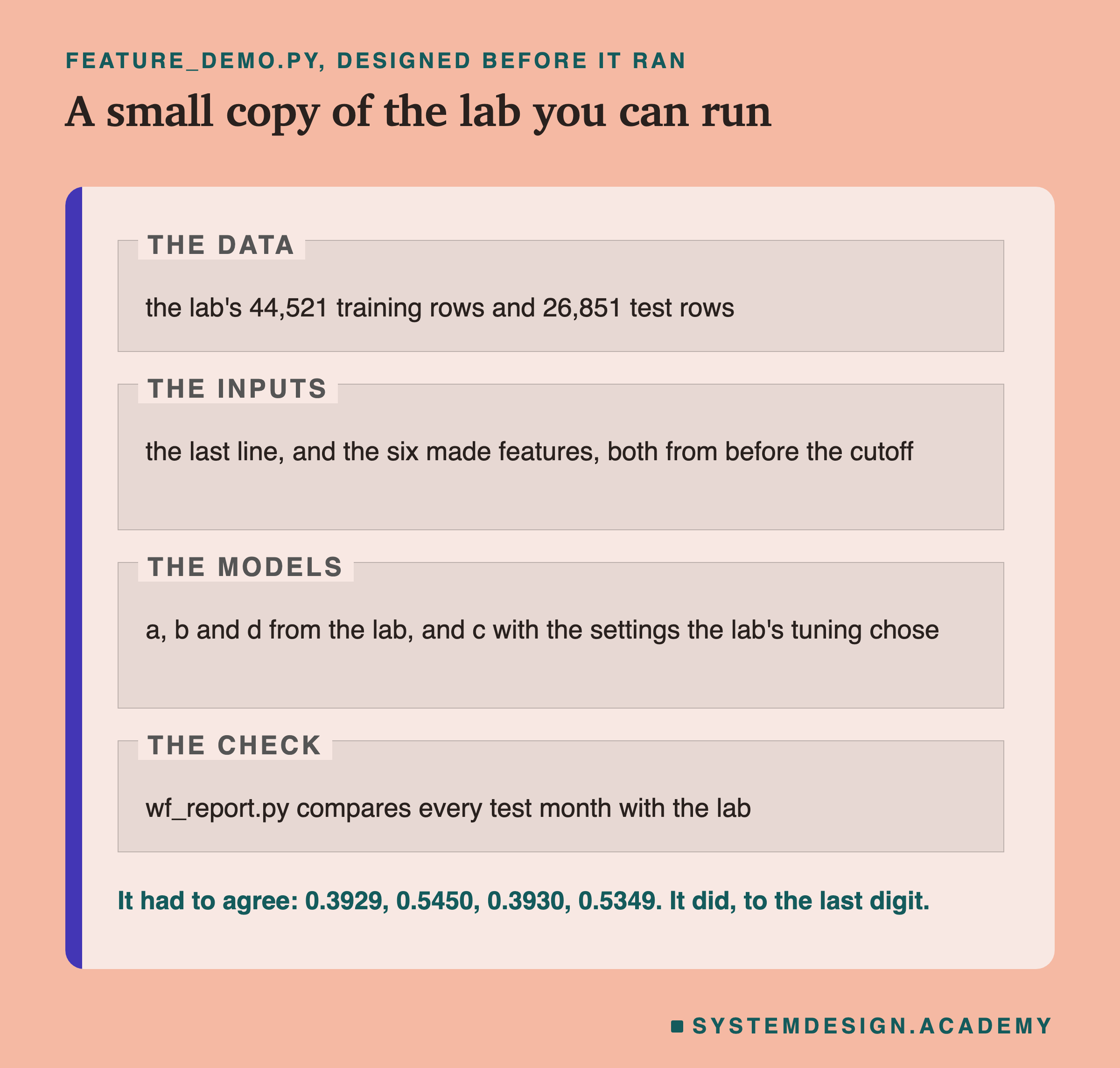
I wrote the demo's design into its docstring after the lab had run and before the demo first ran. It names the four numbers it must reproduce. It skips the tuning, which takes minutes, and uses the settings the lab's tuning chose instead. It says so in its docstring.
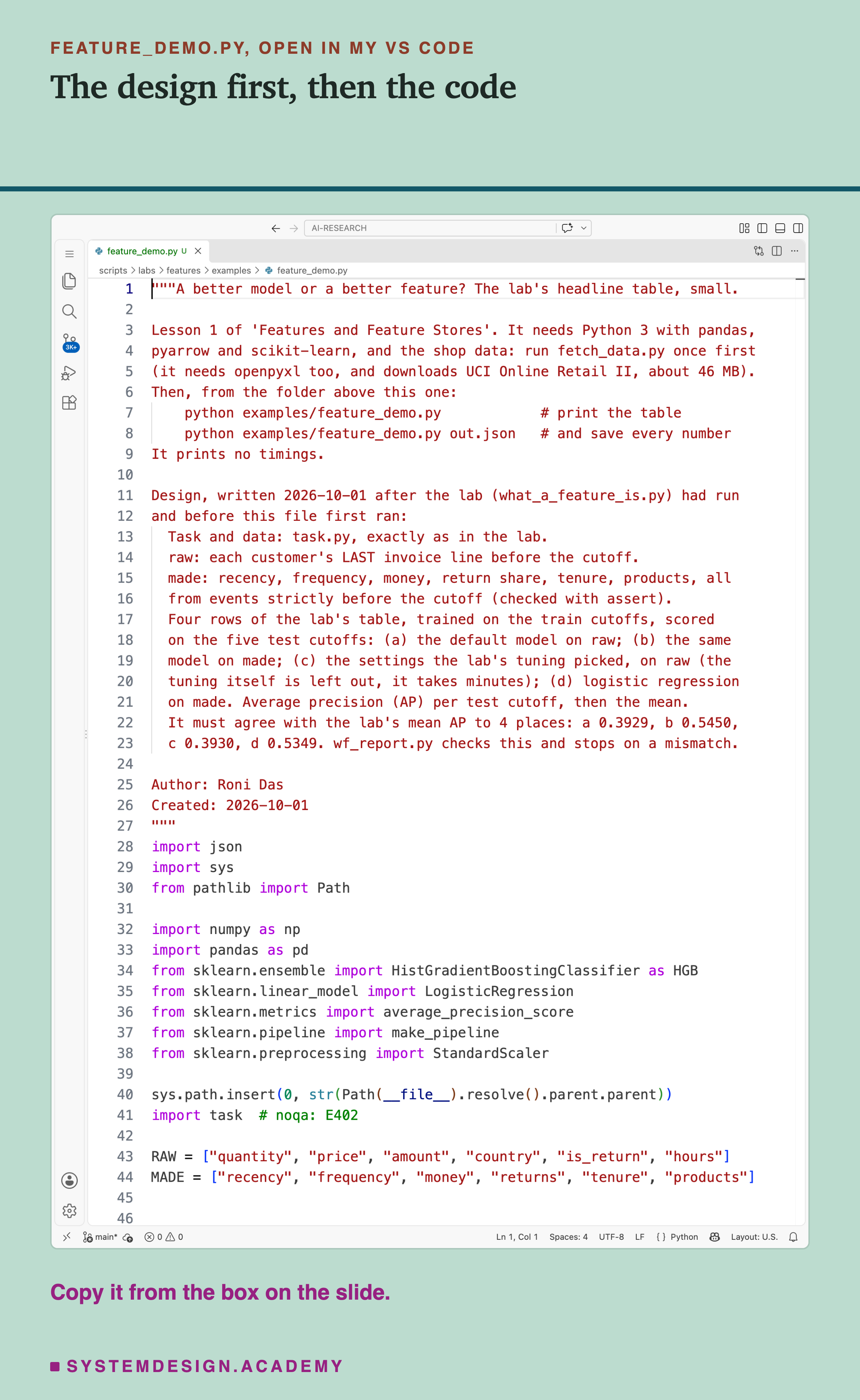
Before you run this lab. You need Python 3 with pandas, pyarrow and scikit-learn: pip install pandas pyarrow scikit-learn openpyxl. First run python fetch_data.py from the scripts/labs/features folder. It downloads the shop data once, about 46 MB, and writes one cleaned file. Then run the demo from the same folder. I ran it with scikit-learn 1.9.1 and pandas 3.0.6 on a Mac. These libraries run on Windows and Linux too, but I have not checked the numbers there. Give it a file name, python examples/feature_demo.py out.json, and it also saves every number. That is how results/wf-demo.json was made.
"""A better model or a better feature? The lab's headline table, small.

Lesson 1 of 'Features and Feature Stores'. It needs Python 3 with pandas,
pyarrow and scikit-learn, and the shop data: run fetch_data.py once first
(it needs openpyxl too, and downloads UCI Online Retail II, about 46 MB).
Then, from the folder above this one:
    python examples/feature_demo.py            # print the table
    python examples/feature_demo.py out.json   # and save every number
It prints no timings.

Design, written 2026-10-01 after the lab (what_a_feature_is.py) had run
and before this file first ran:
  Task and data: task.py, exactly as in the lab.
  raw: each customer's LAST invoice line before the cutoff.
  made: recency, frequency, money, return share, tenure, products, all
  from events strictly before the cutoff (checked with assert).
  Four rows of the lab's table, trained on the train cutoffs, scored
  on the five test cutoffs: (a) the default model on raw; (b) the same
  model on made; (c) the settings the lab's tuning picked, on raw (the
  tuning itself is left out, it takes minutes); (d) logistic regression
  on made. Average precision (AP) per test cutoff, then the mean.
  It must agree with the lab's mean AP to 4 places: a 0.3929, b 0.5450,
  c 0.3930, d 0.5349. wf_report.py checks this and stops on a mismatch.

Author: Roni Das
Created: 2026-10-01
"""
import json
import sys
from pathlib import Path

import numpy as np
import pandas as pd
from sklearn.ensemble import HistGradientBoostingClassifier as HGB
from sklearn.linear_model import LogisticRegression
from sklearn.metrics import average_precision_score
from sklearn.pipeline import make_pipeline
from sklearn.preprocessing import StandardScaler

sys.path.insert(0, str(Path(__file__).resolve().parent.parent))
import task  # noqa: E402

RAW = ["quantity", "price", "amount", "country", "is_return", "hours"]
MADE = ["recency", "frequency", "money", "returns", "tenure", "products"]


def table(ev, labels, cutoffs):
    """One row per (customer, cutoff), from events before the cutoff."""
    out = []
    for t in cutoffs:
        past = ev[ev["ts"] < t]
        assert past["ts"].max() < t
        last = past.groupby("customer_id").tail(1).set_index("customer_id")
        g = past.groupby("customer_id")
        buys = past[~past["is_return"]].groupby("customer_id")
        d = last[["quantity", "price", "amount", "country"]].copy()
        d["is_return"] = last["is_return"].astype(int)
        d["hours"] = (t - last["ts"]).dt.total_seconds() / 3600
        d["recency"] = (t - g["ts"].max()).dt.total_seconds() / 86400
        d["frequency"] = buys["invoice"].nunique().reindex(d.index).fillna(0)
        d["money"] = g["amount"].sum()
        d["returns"] = g["is_return"].mean()
        d["tenure"] = (t - g["ts"].min()).dt.total_seconds() / 86400
        d["products"] = buys["stock_code"].nunique().reindex(d.index).fillna(0)
        d["cutoff"] = t
        out.append(d.reset_index())
    return labels.merge(pd.concat(out), on=["customer_id", "cutoff"])


ev = task.load_events()
lab_tr, _, lab_te = task.splits(ev)
tr = table(ev, lab_tr, task.TRAIN_CUTOFFS)
te = table(ev, lab_te, task.TEST_CUTOFFS)
codes = {c: i for i, c in enumerate(sorted(tr["country"].unique()))}
for d in (tr, te):
    d["country"] = d["country"].map(codes).astype(float)

cat = [c == "country" for c in RAW]
models = {
    "a  default model, raw columns": (HGB(random_state=0, categorical_features=cat), RAW),
    "b  default model, made features": (HGB(random_state=0), MADE),
    "c  tuned model, raw columns": (HGB(random_state=0, categorical_features=cat, learning_rate=0.03,
                                      max_leaf_nodes=7, min_samples_leaf=400, max_iter=500), RAW),
    "d  logistic, made features": (make_pipeline(StandardScaler(),
                                   LogisticRegression(max_iter=2000)), MADE),
}
cut = te["cutoff"].dt.strftime("%Y-%m")
rates = te.groupby(cut)["label"].mean()
print(f"test rows {len(te):,}; train rows {len(tr):,}")
print("average precision (AP) on each test cutoff")
print(f"{'':32s}" + " ".join(c[2:] for c in rates.index) + "   mean")
print(f"{'base rate (share who buy)':32s}" + " ".join(f"{v:.3f}" for v in rates) + f"  {rates.mean():.4f}")
results = {"base_rate": rates.to_dict()}
for name, (model, cols) in models.items():
    model.fit(tr[cols], tr["label"])
    te["p"] = model.predict_proba(te[cols])[:, 1]
    ap = te.groupby(cut)[["label", "p"]].apply(
        lambda d: average_precision_score(d["label"], d["p"]))
    results[name[0]] = ap.to_dict()
    print(f"{name:32s}" + " ".join(f"{v:.3f}" for v in ap) + f"  {np.mean(ap):.4f}")

if len(sys.argv) > 1:
    json.dump(results, open(sys.argv[1], "w"), indent=1)
Compare Any Two Contestants Yourself
This box holds the lab's real average precision for every contestant, one number for each of the five test months, plus the base rate of each month. Press Run to compare the tuned raw model with the default model on made features.
Then find the line that starts with A, B =, near the top. Change the two letters inside the quotes, keep the quotes, and press Run again. Try "a" and "c" to see what tuning bought, or "b" and "e".
The box prints the two contestants side by side for each month, the gain, and how many months the second one won. Each value is copied from wf-result.json at the full precision the lab stored. The report script writes this box from that file, runs it, and checks that it prints the lab's means.
Common Mistakes, and When Each Choice Helps
Reaching for a bigger model first. Here, 78 settings of gradient boosting and random forests squeezed 0.0001 out of the raw last line with seed 0, and 0.0023 on average over 20 seeds. When a model is weak, first ask what it is being shown.
Building a feature from the future. A feature like "total spend" is easy to compute over the whole table by accident, including the months after the cutoff. Then the lab score is a lie. Build every feature from events before the cutoff, and assert it in code, the way this lab does.
Choosing settings on the test months. If I had kept the setting that scored best on the test months, I would have reported a gain that new months would not repeat. Choose on valid months only.
Believing one seed. A model's own randomness moved its mean test score by up to 0.010 here. Compare models seed by seed, or treat a gap smaller than that with care.
Comparing AP across months. A month with more buyers is easier. Compare contestants within one month, or over the same months.
When made features help most. When each row is one event, but the question is about a person, a machine or an account over time. Then the useful signal lives in counts, sums and gaps across many rows, and a single row cannot hold it.
When a better model helps more. When your features already carry the signal, and the pattern between them is complicated. Here the made features were simple enough that even a straight-line model came close.
What This Lab Cannot Tell You
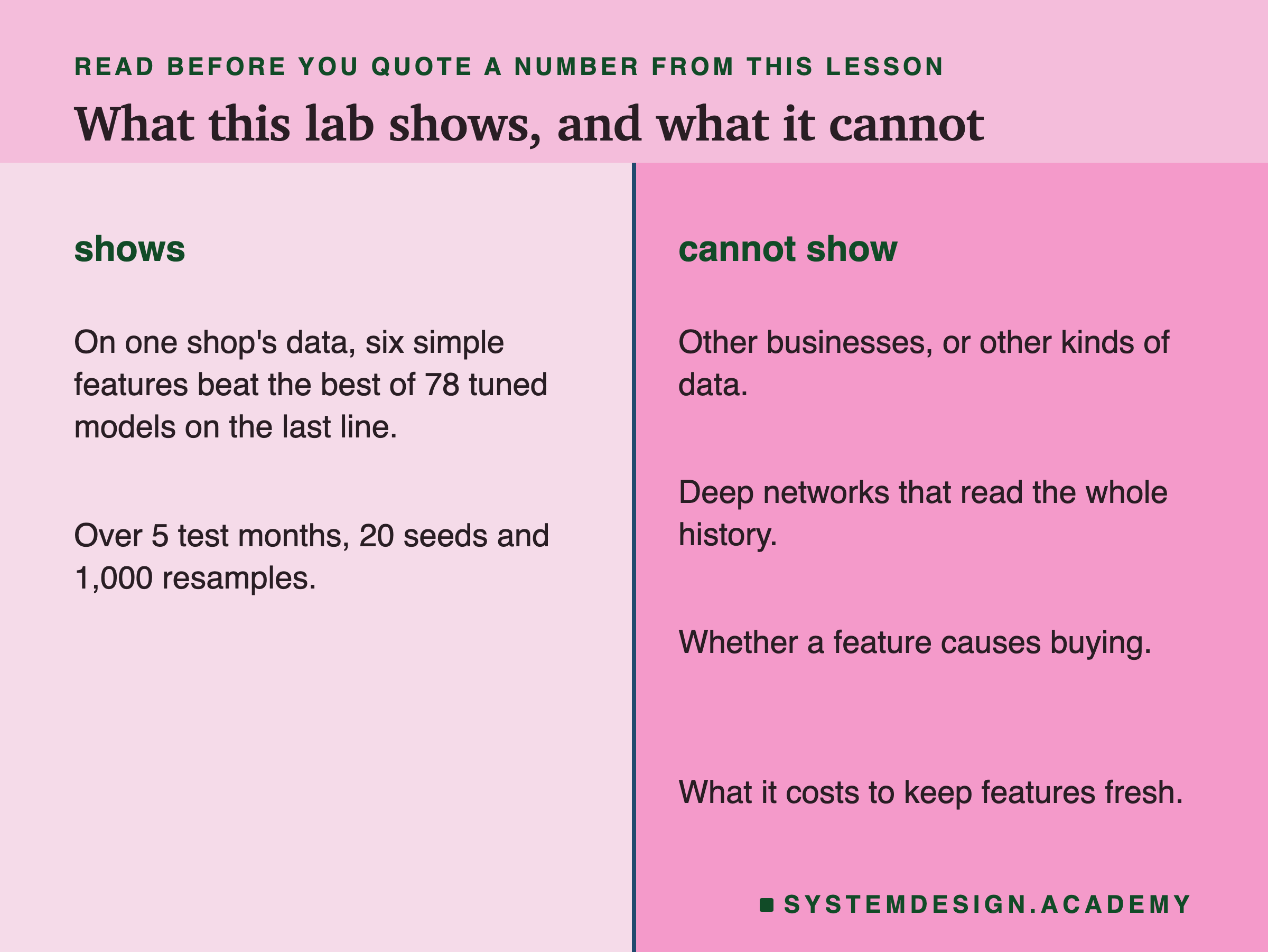
One shop, one task. A gift shop with many wholesale buyers, and one question: will they buy within 30 days? Other businesses and other questions may behave differently.
A deliberately thin raw view. The raw contestants saw only the last line. A model that reads a customer's whole sequence of lines, such as a neural network built for sequences, might learn its own version of frequency. I did not test one. The fair conclusion is narrower: given one row, hand the model a summary of the history.
Features, not causes. Frequency predicted buying best. That does not mean making someone order more often would make them come back. The data shows what goes together, not what causes what.
Tuning was limited to 78 settings. Both winners sat at the edge of their grid, so a wider search might find a little more on the raw columns. Given how flat the 78 were, I doubt it would close a 0.152 gap, but that is a guess, not a measurement.
The follow-up came after the results. The single-feature and drop-one numbers were asked after I saw the headline, and each ran with one seed.
Cost. Made features have to be computed, stored and kept fresh, and the rest of this chapter is about that cost. This lesson measured only what they are worth.
What to Do on Monday
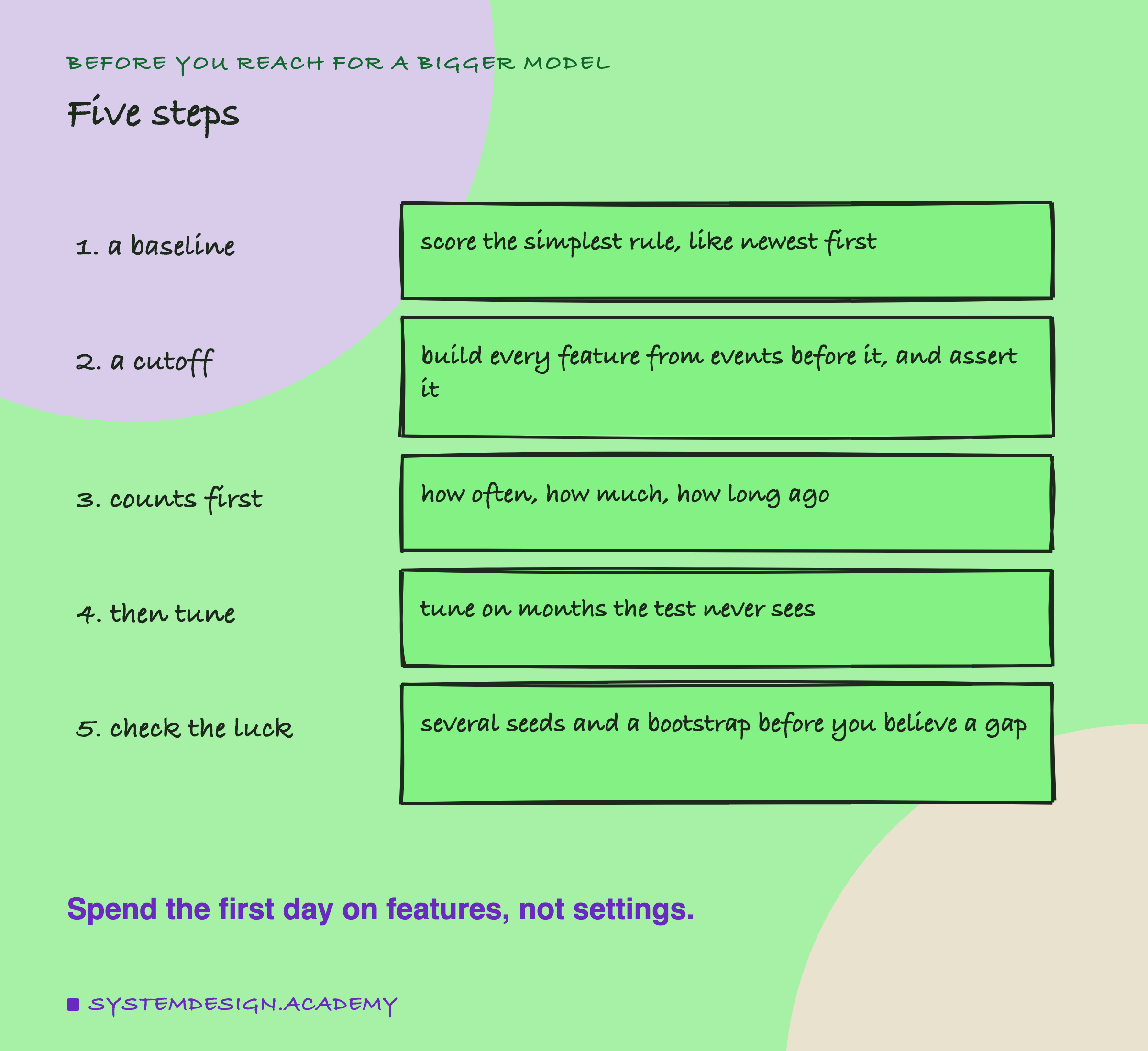
These are the five steps I would take on a new prediction task, in the order I would take them. Each one comes from something this lab measured, and the list below says what.
-
Score a baseline with no model. Here, sorting by recency scored 0.380. Any model has to clearly beat that to be worth running.
-
Fix the cutoff and assert it. Decide the moment of the guess, and make the code fail if a feature reads past it.
-
Start with counts. How often, how much, how long ago, how long known. These are cheap to compute and, here, they carried almost all the gain.
-
Then tune, on separate months. Tune after the features, and choose on months the test never sees.
-
Check the luck. Retrain with several seeds and bootstrap the test rows before you believe a gap. Here the feature gap was huge next to both kinds of luck. The tuning gap was real over 20 paired seeds, but smaller than the seed-to-seed wobble of either model.
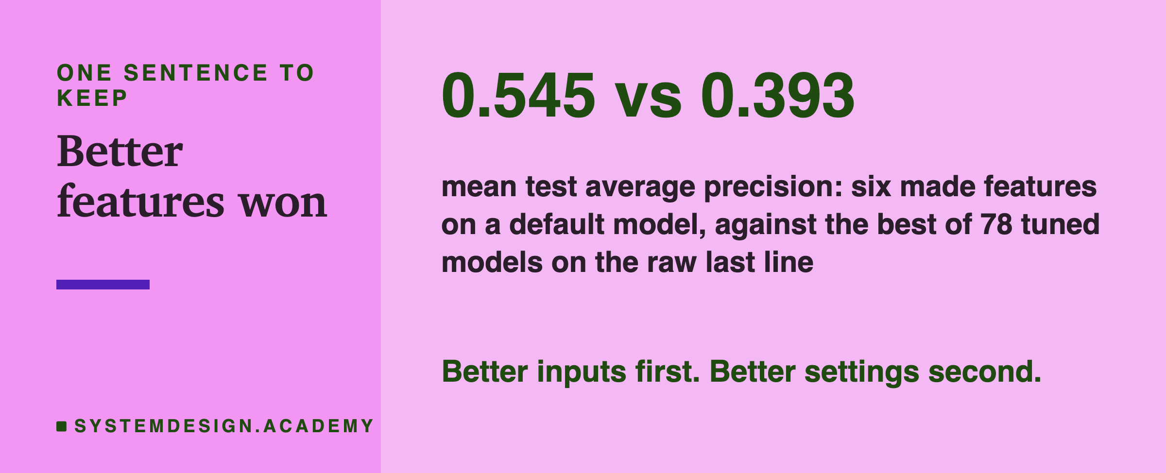
The one idea to keep: on this data, what I handed the model mattered far more than how I tuned it. The rest of this chapter is about handing it the right values, at the right moment, in training and in the live app alike.
Knowledge Check
Knowledge Check
4 questions - Score 80% to pass
In this lab, what happened when the model on the raw last line was tuned over 78 settings?
Why does a random order of customers score an average precision near 0.196 here, not near zero?
Why did the best of 78 settings score 0.362 on the valid months but no better than the default on the test months?
What does the follow-up run, asked after the results, suggest about which made feature did the most?