A Test With Tomorrow's Notes
A friend says he can guess which of your neighbours will go to the corner shop next week. You want to test him. So you keep a notebook about each neighbour: how often they went to the shop, how much they spent, when they last went. On the first of the month you plan to hand him the notebook, as it was that morning, and ask him to guess.
But you are busy, and you test him a year later. You hand him the notebook as it is now. The pages now say things like "went to the shop on the 7th". He reads them, and he guesses almost perfectly.

Was he good at guessing? You cannot tell. The notebook you gave him already held part of the answer. Next month, when you ask him for real, he will only have the notebook as it is on that day, and his guesses will be much worse.
Machine learning teams make this mistake with real data, and the person in the picture above is often the one who shows the too-good score in a meeting. In this lesson I measure how much it inflates the score, on real data from a real shop. Then I measure how far the score falls when the model meets the future for real.
Where This Lesson Starts
The previous lesson, what a feature is, introduced this chapter's data and its one prediction task. This lesson keeps both and asks one question about them.
The feature stores lesson in the foundation course explains point-in-time correctness in words: each training row must see only the values that existed at its own moment. It also has a tiny example with four made-up numbers. I will not repeat it. Here I measure the same idea on 44,521 real training rows, with a real model, and put numbers on the damage.
The lesson on leakage before the split is the closest relative. It measured leaks from preparation steps that run before the data is split. It also named one leak it did not test: columns that hold information from after the moment of prediction. This lesson tests exactly that leak, in the form it usually takes in practice, a careless join.
The question is simple. If a team builds its training table by joining each customer's latest feature values, how much better does the model look offline than it really is?
The Words You Need First
Please read this slide slowly if any word is new. Every slide after it uses these words.
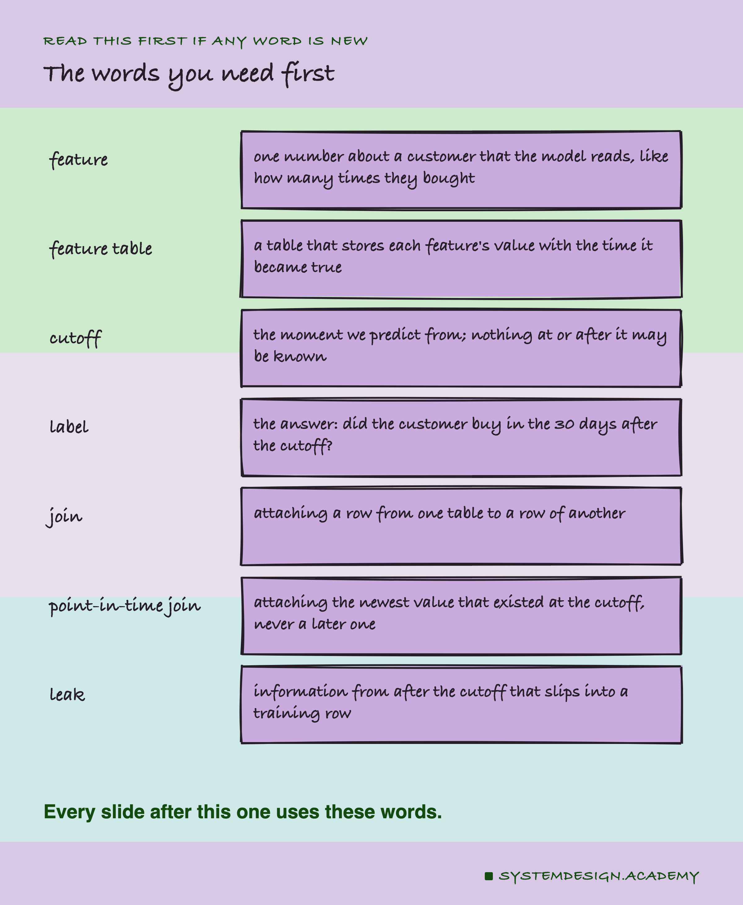
Feature. One number about a customer that the model reads, such as how many times they have bought. The model learns from features, not from raw records.
Feature table. A table that stores each feature's value together with a timestamp: the time from which that value is true. When the value changes, the table gets a new row. The old row stays, so the table holds the whole history.
Cutoff. The moment we make a prediction from. Nothing that happened at or after the cutoff may be known to the model. In this lesson the cutoffs are the first of each month at midnight.
Label. The answer the model learns to predict. Here: did the customer buy anything in the 30 days starting at the cutoff, yes or no.
Join. Attaching a row from one table to a row of another, matched by something they share, here the customer's id.
Point-in-time join. A join that takes, for each training row, the newest feature row that already existed at that row's cutoff. It is also called an as-of join, because it asks "what was true as of this time?".
Latest-value join. A join that takes each customer's newest feature row in the whole table, whatever the cutoff. It is what you get from a query that asks for the current values.
Leak. Information from after the cutoff that slips into a training row.
How I Score a Model
Two more words, because every result slide uses them.
Average precision (AP). The model gives every customer a score: how likely they are to buy. Sort the customers from highest score to lowest. Walk down the list. Each time you reach a real buyer, note what share of the customers so far were buyers. Average those shares. A perfect model puts all the buyers first and scores 1.
A model that sorts at random scores about the share of buyers in the data, which I call the random guess. I work out AP separately for each cutoff and then average, so every month counts the same. Averaged over the test months, the share of buyers is 0.196, so 0.196 is the floor to beat.
ROC-AUC. Pick one real buyer and one customer who did not buy, at random. ROC-AUC is the chance that the model gives the buyer the higher score. A coin flip gives 0.5 and a perfect model gives 1. It does not move when the share of buyers changes, which AP does, so I report both.
Hold-out. Rows kept aside while the model learns, then used to score it. A random hold-out is a random 20 percent of the rows.
Seed. A number that fixes a random draw, so it can be repeated exactly. I draw the random hold-out 20 times, with seeds 0 to 19, and report the spread, so one lucky draw cannot fool me.
Offline score. The score a team sees before launch, on a hold-out from its own training table. Serving. Running the model on live data, after launch.
The Shop, the Customers and the Question
The data is UCI Online Retail II, a public dataset under a CC BY 4.0 licence, which lets anyone use it as long as they credit the source. It holds every sale of a UK online shop from 1 December 2009 to 9 December 2011. After this chapter's fixed cleaning, which drops lines with no customer id and keeps returns as flagged rows, it has 44,876 invoices from 5,942 customers. An invoice is one order, and a return is an invoice whose number starts with "C".
The question is the chapter's fixed one. On the first of a month, for every customer who had bought or returned anything before that day, will they buy again in the next 30 days?
Each pair of a customer and a cutoff is one row. The training rows come from 13 cutoffs, March 2010 to March 2011: 44,521 rows, and 23.4 percent of them bought. The test rows come from 5 later cutoffs, July to November 2011: 26,851 rows, and 19.7 percent bought, which averages to 0.196 when each month counts the same. Three cutoffs in between, April to June 2011, are a validation set, a set kept for checking choices. This lab makes no choices, so it only records their scores. On them, per cutoff, the point-in-time model scored an AP of 0.500 and the latest-value model 0.284.
The test cutoffs are never used to choose anything. They stand in for the months after launch.
The Feature Table, as a Nightly Job Writes It
A real feature table is usually written by a job that runs on a schedule, often once a night. I built mine the same way.
For every customer, on every day they had at least one invoice, the job writes one row. The row holds running totals over all of that customer's invoices up to the end of that day:
- frequency: how many buy invoices so far.
- money: how much they have spent so far, in pounds.
- return share: returns divided by all invoices so far.
- last buy: the time of their latest buy so far.
Each row also gets a timestamp, which I call "valid from". It is midnight after the day the row covers, the moment the night's job has seen the whole day. A day with no invoices writes no row, because nothing changed. That gives 38,502 rows for 5,942 customers.
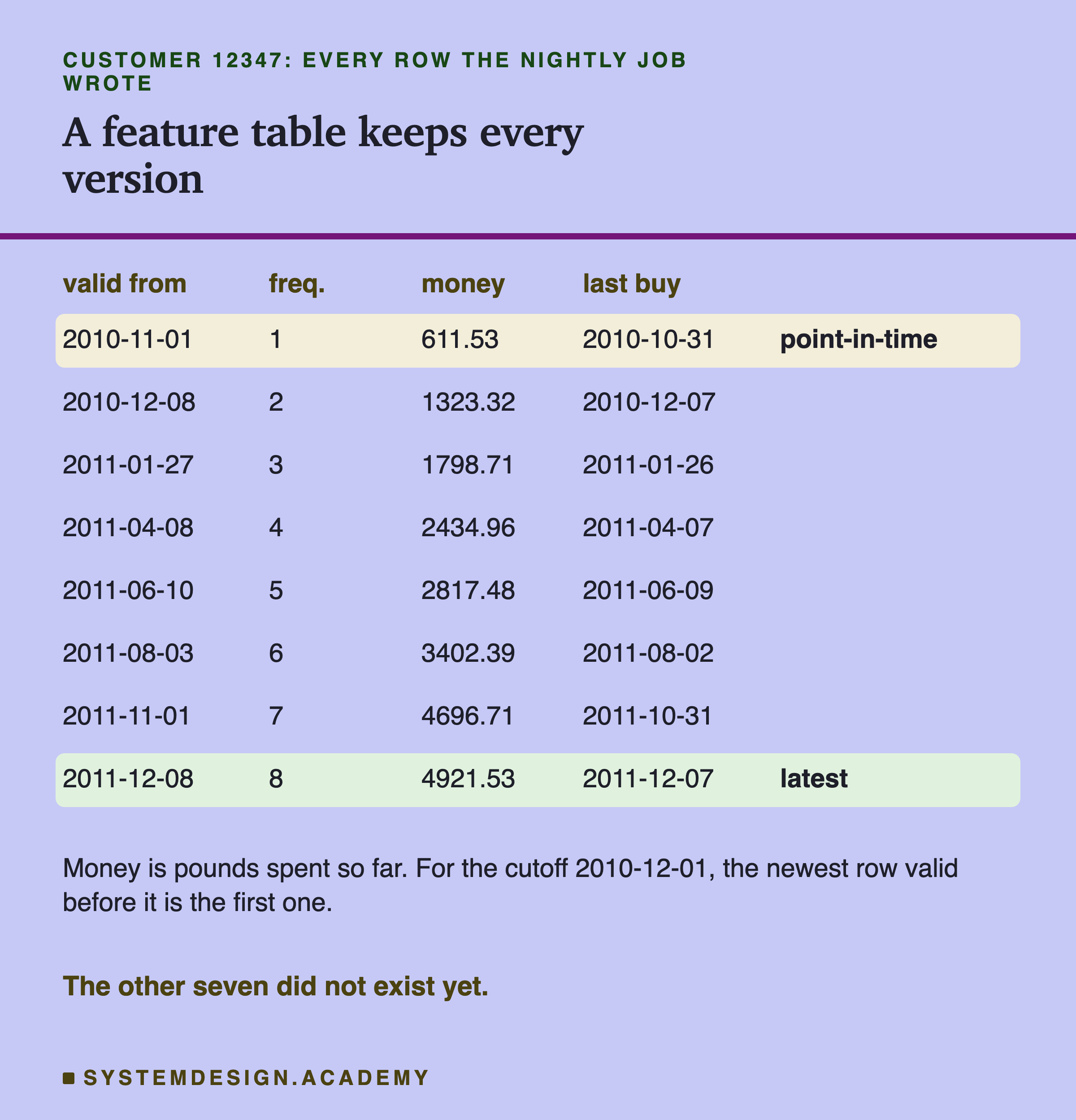
Here is the whole table for one real customer, number 12347. This is a public dataset, so a real id is fine. The customer bought eight times in two years, and each buy added a row. Notice that no old row is ever changed. The table remembers what was true on each day, which is exactly what a point-in-time join needs.
Recency is not stored. Recency, the number of days since the last buy, changes every single day, even when the customer does nothing. Storing it would need a row for every customer on every day. So the table stores the time of the last buy, and recency is worked out at join time: the cutoff minus the last buy. This is a common pattern, and it matters later, because it is where the most obvious leak shows up.
Three Ways to Join the Same Table
Now the training rows need features. Each row is a customer and a cutoff, and the table has many rows per customer. Which one should it take? The lab tries three answers.
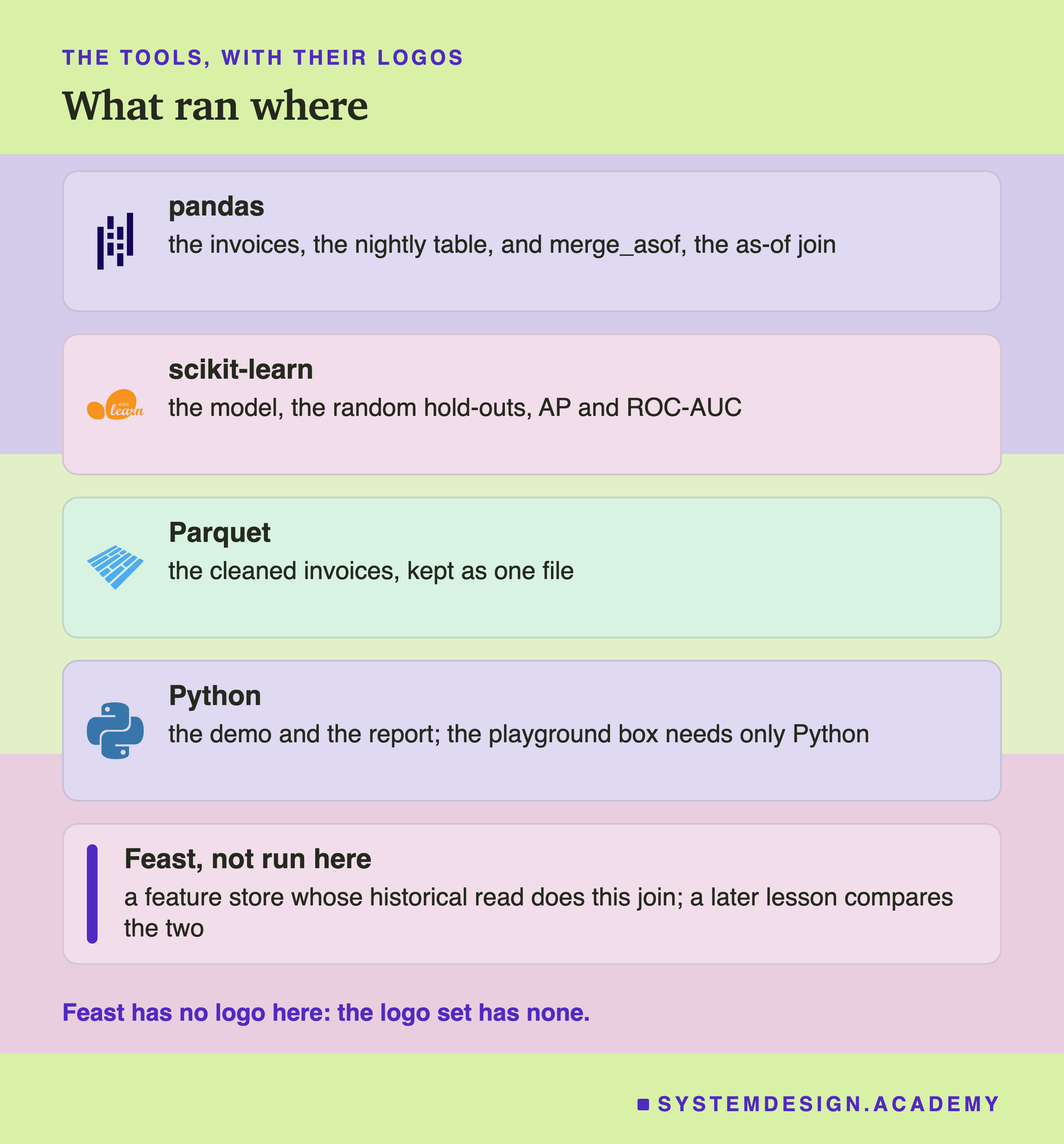
(a) Point-in-time. Take the newest row whose "valid from" is at or before the cutoff. In pandas, the most common Python library for tables, this is one call: pd.merge_asof, matched by customer, looking backward in time from the cutoff.
(b) Latest value. Take the customer's newest row in the whole table, whatever the cutoff. This is what a team gets when it asks a feature table for its current values and attaches them to old training rows.
(c) Off by one day. The same rows as (a), but stamped with the start of the day they cover instead of the end. I come back to this one later.
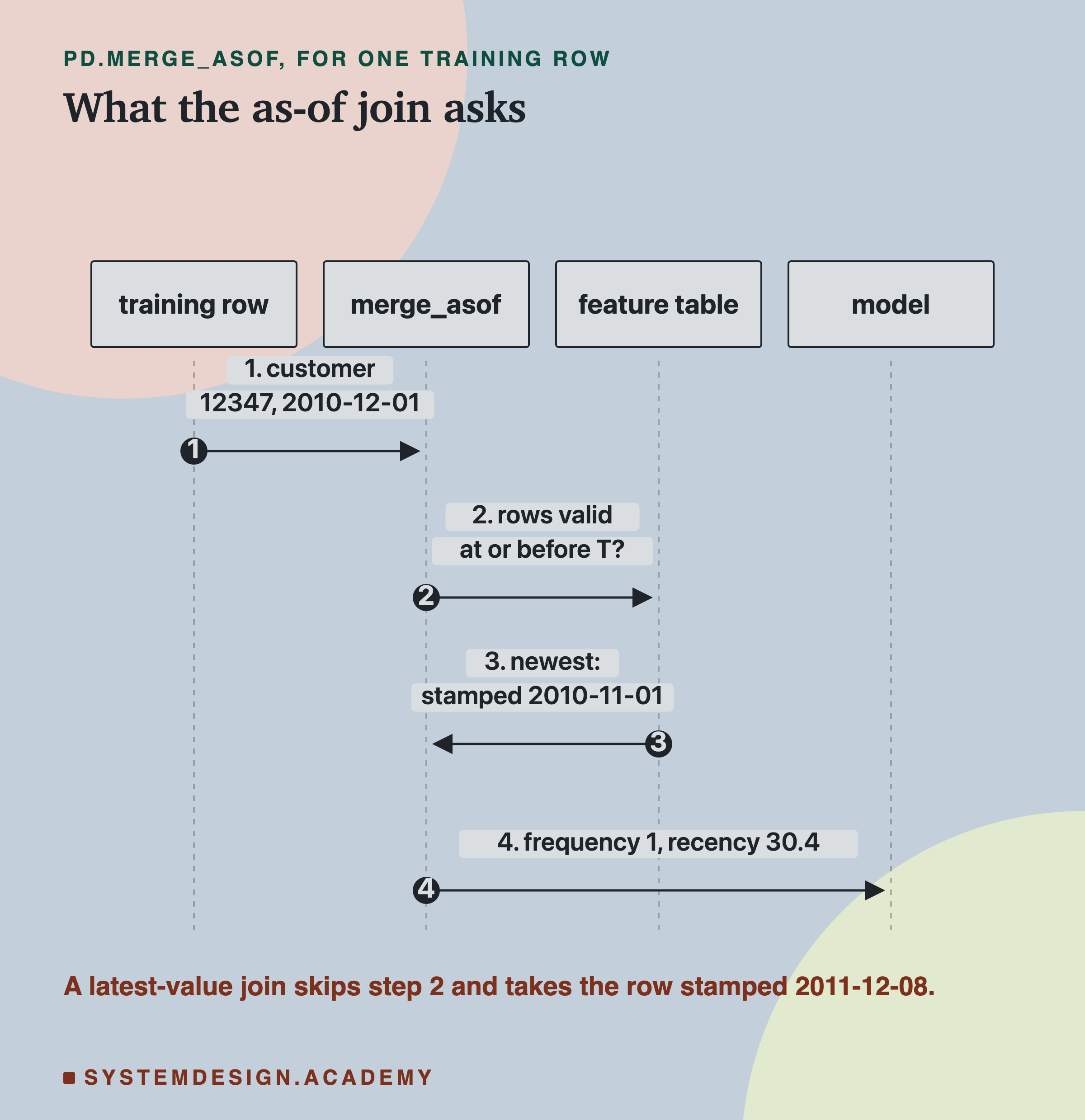
Here is what the as-of join does for one training row. Step 2 is the whole idea: it only looks at rows that already existed. A latest-value join never asks that question.
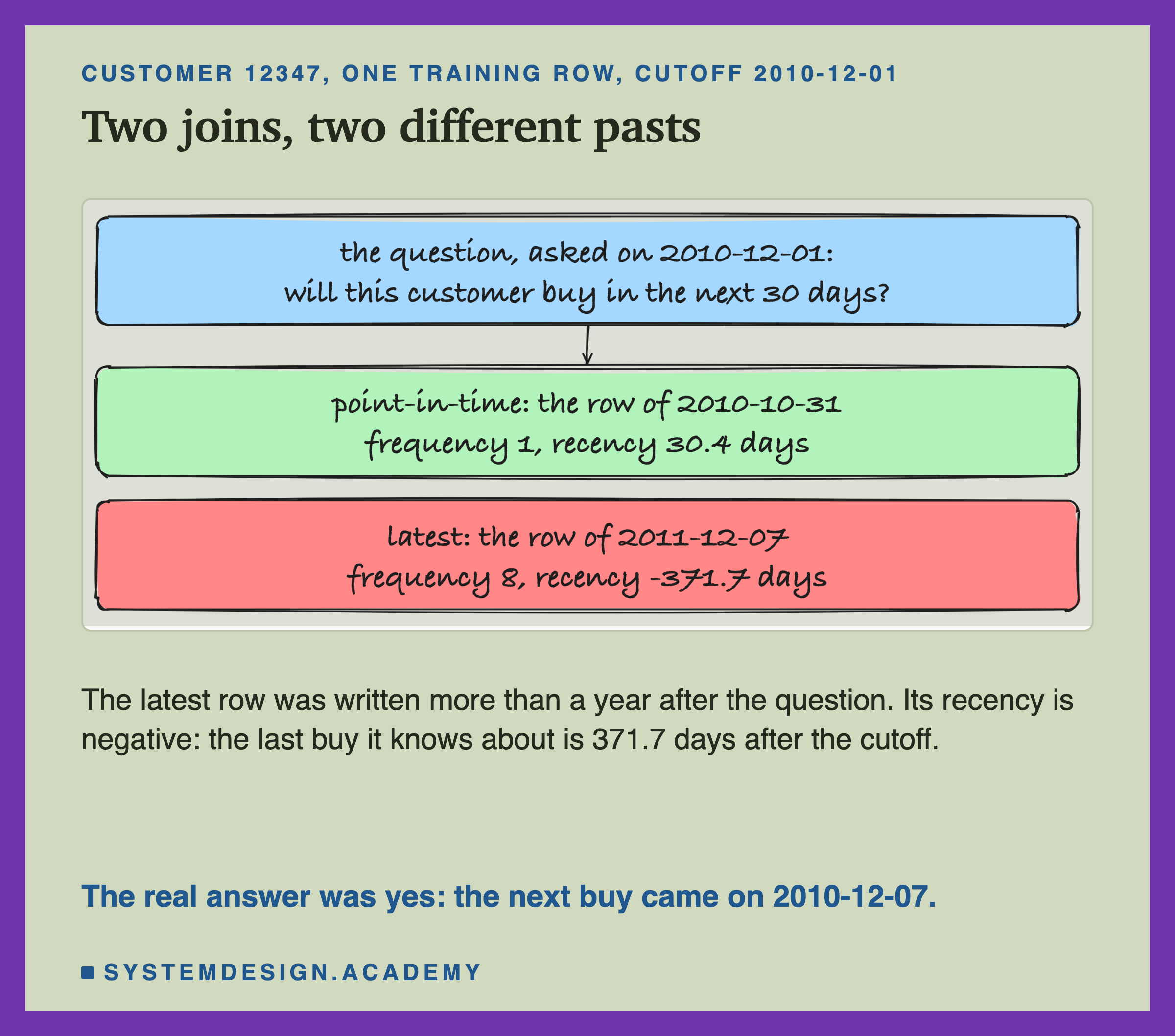
For customer 12347 at the cutoff 1 December 2010, the two joins give very different rows. Point-in-time says: one buy so far, the last one 30.4 days ago. Latest value says: eight buys, the last one 371.7 days in the future, which shows up as a negative recency of -371.7. The latest row also counts the buy of 7 December 2010, the very buy the label is asking about.
The Same Choice, Drawn as Blocks
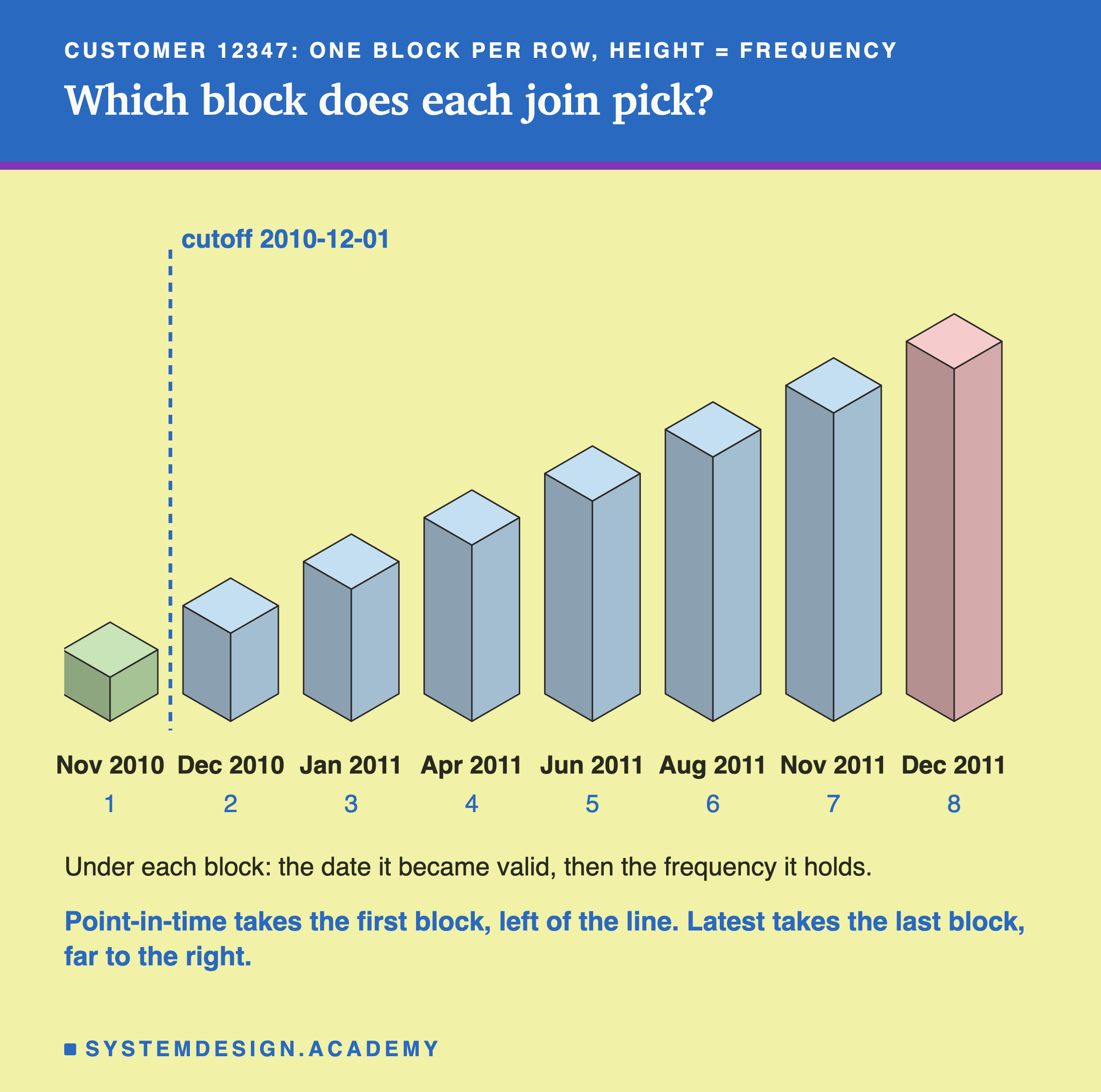
Think of the feature table as a shelf of blocks, one per version, placed in time order. The cutoff is a line across the shelf. A point-in-time join may only reach to the left of the line, and takes the nearest block there. A latest-value join reaches to the far end of the shelf, wherever the line is.
The blocks also show why the leak is worse for some rows than others. For a cutoff late in the data, the last block is close to the line and holds little extra. For an early cutoff, like this one, the last block is a year away and holds a year of buying. The training rows in this lab come from cutoffs in 2010 and early 2011. The table runs to December 2011, so most training rows sit far from the end of the shelf.
How the Lab Was Built
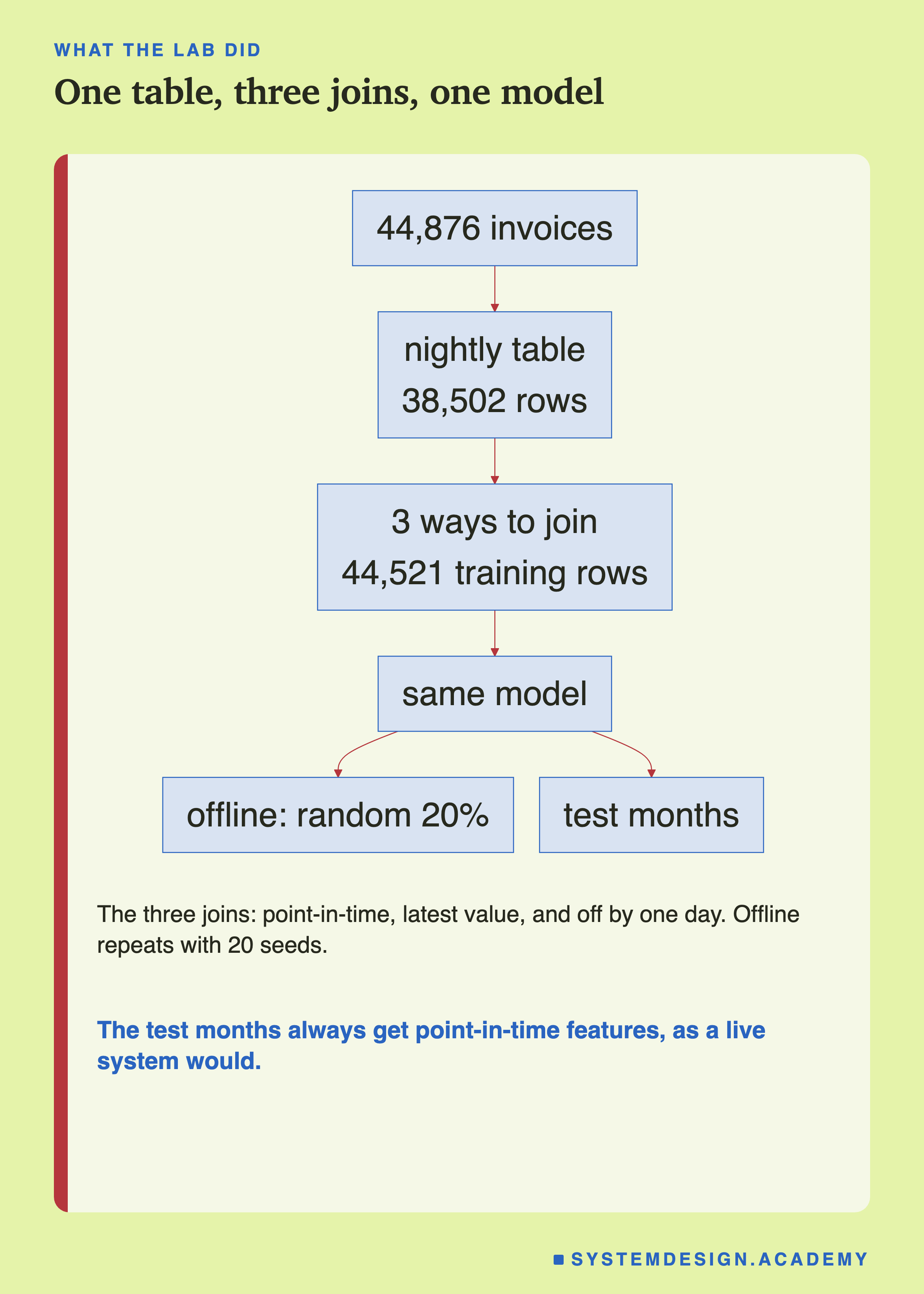
I wrote the lab's design into the docstring of scripts/labs/features/point_in_time.py before it ran. A docstring is the note at the top of a Python file. The design fixed the table, the three joins, the counts, the model and every score below. Nothing in it was chosen after seeing a result, except the changes a review asked for, which the docstring and this lesson label.
-
A check first. Before any model, the lab recomputes all four features for every training, validation and test row. It works straight from the raw invoices before each cutoff, with no feature table at all. The point-in-time join must agree with that on every value. It does, on 344,180 values.
-
The model. HistGradientBoostingClassifier from scikit-learn, a common library for this kind of model, with
random_state=0and its other settings left at their defaults. It grows many small decision trees, chains of yes-or-no questions about the columns, each tree fixing the mistakes of the ones before. One default matters: above 10,000 rows it turns on early stopping, which keeps 10 percent of the training rows aside to decide when to stop adding trees. Every training table here is above that size, so it is on in every fit. -
The offline score. On each join's own training table: hold out a random 20 percent, train on the other 80, score the 20. The score is worked out for each of the 13 training cutoffs and averaged, the same way as the test months. Twenty seeds.
-
The serving score. Train once on the whole table, then score the five test cutoffs. The test rows always get point-in-time features, because a live system can only read values that exist when it predicts.
The Lab, Rebuilt and Checked
This is a real recording of the report script, pit_report.py, run on the laptop where the lab ran. It does not trust the lab. It rebuilds every number from the raw invoices with its own code, and stops on the first one that does not match.
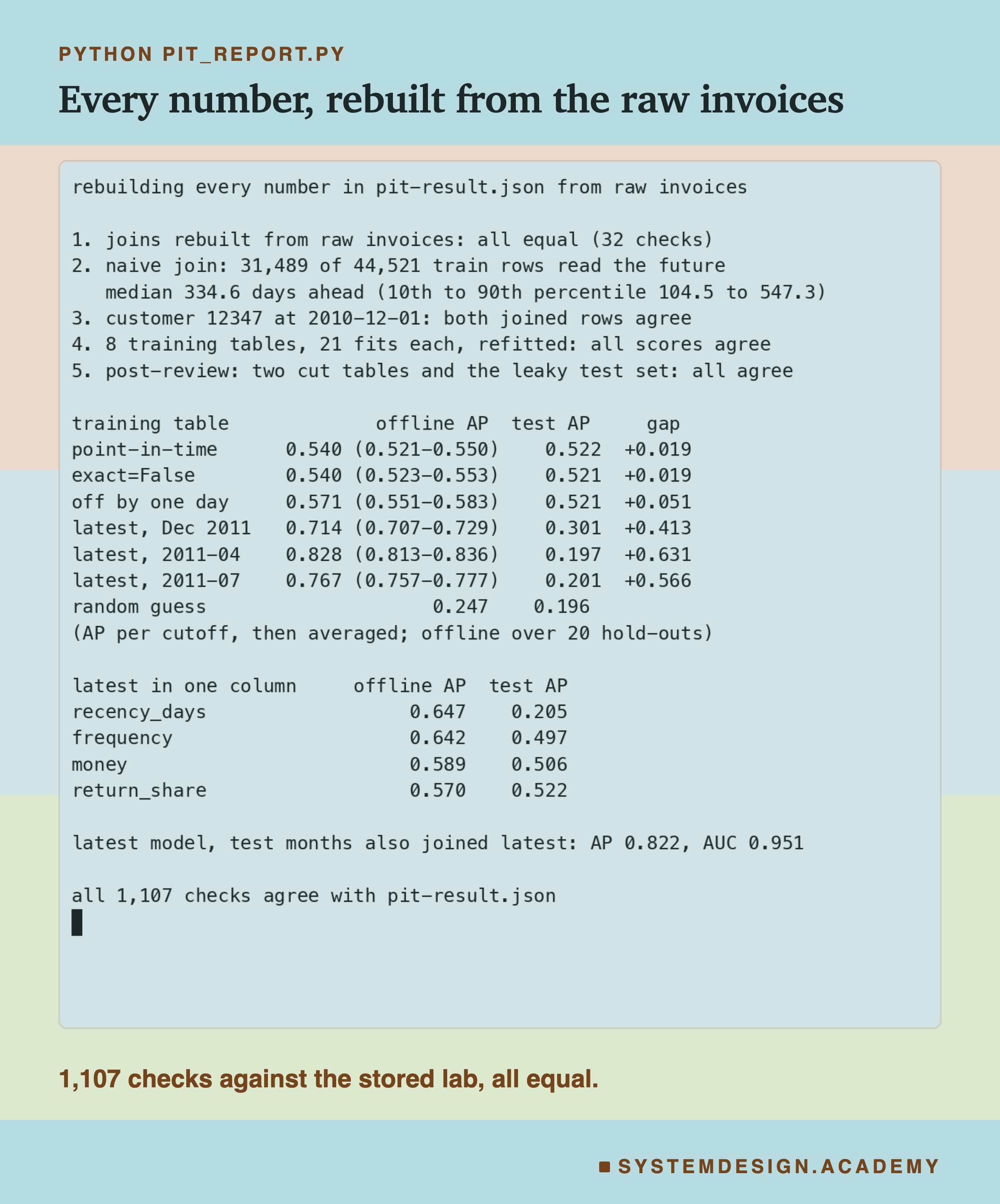
The report's trick is that every join in this lab is the same question with a different time limit. Point-in-time uses the invoices before the cutoff. Latest value uses every invoice in the data. Off by one day uses the invoices before the end of the cutoff day. So the report can rebuild each join's features straight from the invoices, with no feature table and no merge_asof, and compare.
It then refits every model. One honest detail: my first version refitted on its own rebuilt columns and failed at hold-out seed 3, in the sixth decimal place. Money added up in a different order differs around the thirteenth digit, and that was enough to move one internal boundary inside the model. So the report now proves the columns equal first, then refits on the lab's columns.
In the recording, "latest, Dec 2011" is the latest-value join. The two other "latest" rows are tables built earlier, which a later slide covers. "exact=False" is a setting I explain later. "10th to 90th percentile" means the range that holds the middle 80 percent of the rows.
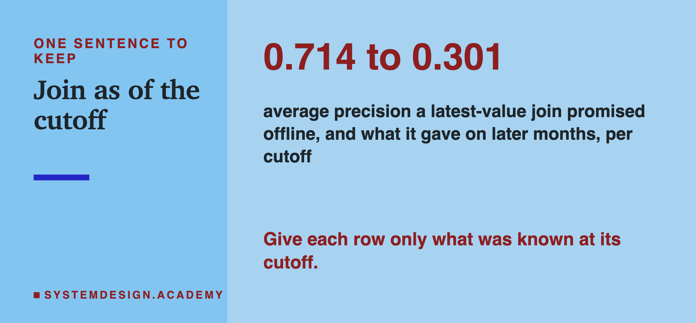
Promised 0.714, Delivered 0.301
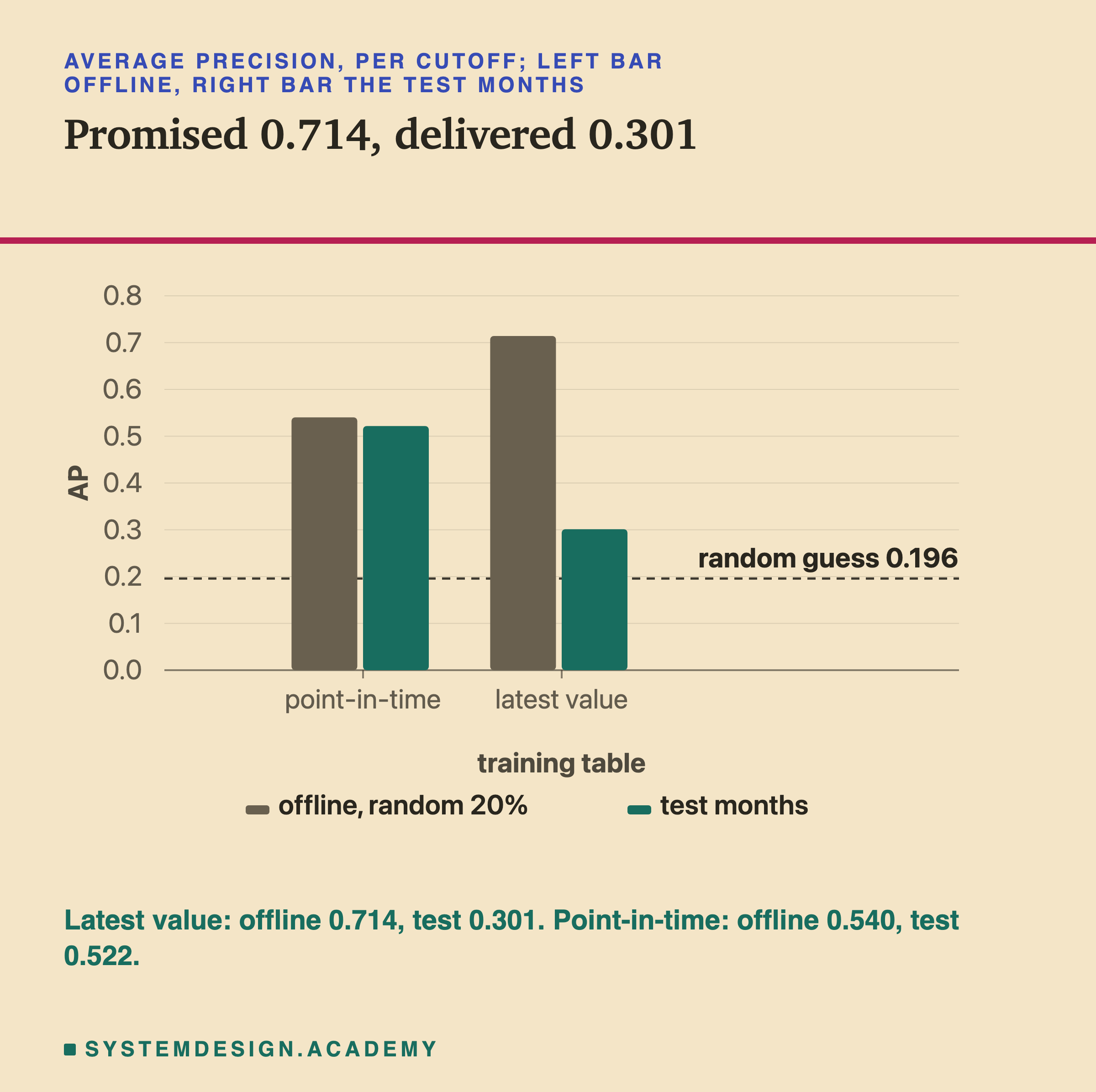
Here is the headline. The first number is what a team would see offline. The second is what the same model gave on the later test months.
| training table | offline AP, 20 seeds | test months AP |
|---|---|---|
| point-in-time | 0.540 (0.521 to 0.550) | 0.522 |
| latest value | 0.714 (0.707 to 0.729) | 0.301 |
| random guess | 0.247 | 0.196 |
Every AP here is worked out per cutoff and then averaged. The latest-value table promised an average precision of 0.714. The test months gave 0.301, a gap of 0.413. That is closer to a random guess, 0.196, than to the honest model.
The point-in-time table promised 0.540 and gave 0.522, a small drop of 0.019. A random hold-out from earlier months is not the same as later months, so some drop is expected, and it is not a leak.
So the leak did two things. It made the offline score look 0.174 better than the honest table's offline score. And it made the real model worse: on the test months, the honest model beat it by about 0.22.
The random-guess row differs between the columns because AP's floor is the share of buyers, and the training months had more buyers than the test months.
Not One Lucky Draw
A random hold-out is one draw. A different seed puts different rows in it, and the score moves. So I drew it twenty times.
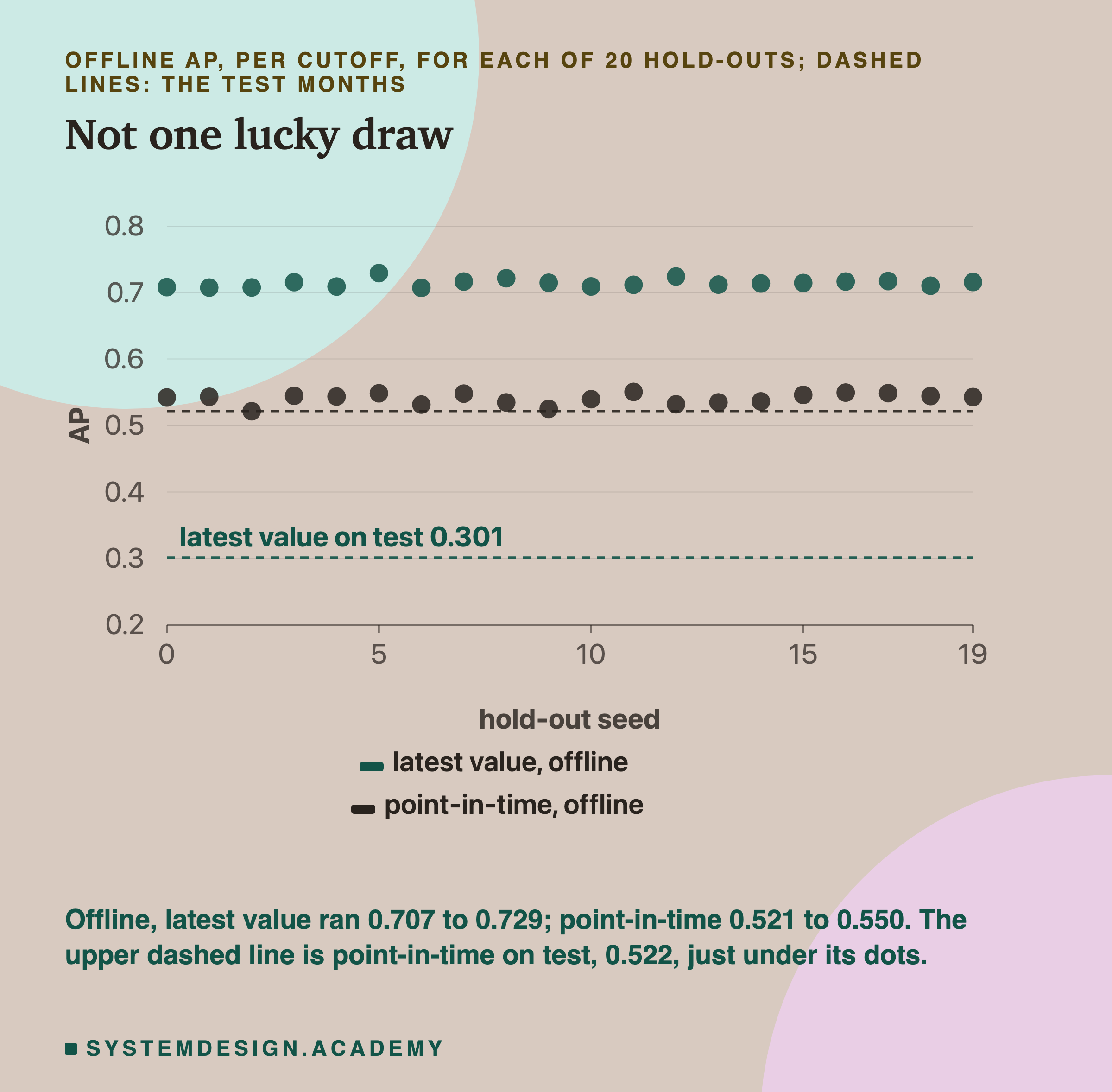
Across the 20 seeds, the latest-value table's offline AP ran from 0.707 to 0.729. The point-in-time table's ran from 0.521 to 0.550. The two bands do not touch: the lowest latest-value seed is above the highest point-in-time seed.
The test scores have no seed spread, because the model is trained once with random_state=0 and the test months are fixed. The serving score of the latest-value model, 0.301, sits far below every one of its own offline dots. None of the 20 hold-outs came close to the truth. The point-in-time model's test score, 0.522, sits just under its dots: 19 of its 20 seeds scored a little higher offline.
This is what makes it dangerous. Repeating the offline check more carefully does not help. Every random hold-out is cut from the same leaky table, so every one of them leaks in the same way.
The Same Story on a Second Score
AP depends on how many buyers there are, and the training months had more buyers than the test months. So I also report ROC-AUC, which does not move with that share.
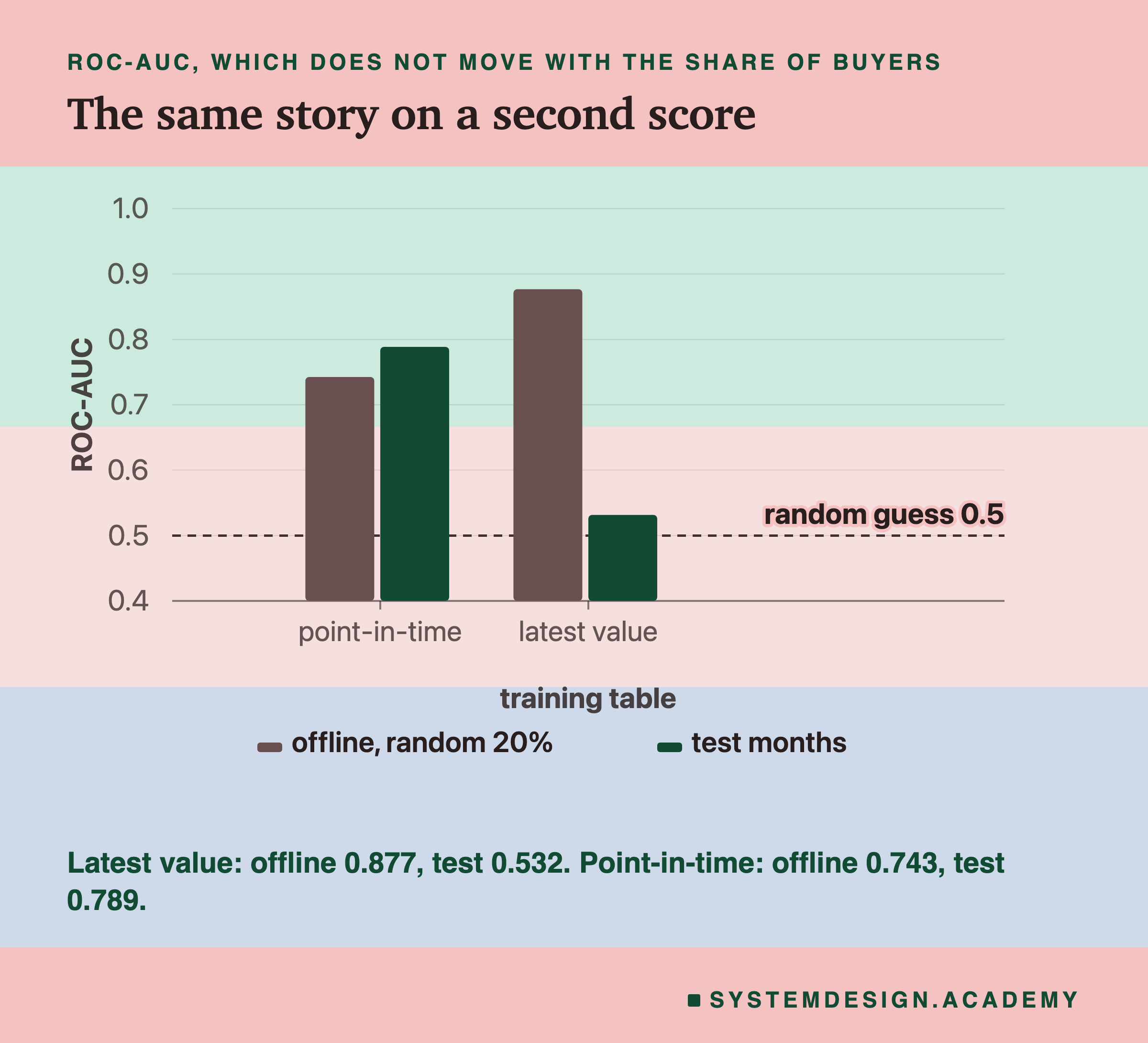
On ROC-AUC, also per cutoff, the latest-value table promised 0.877 and gave 0.532 on the test months, just above a coin flip at 0.5. The point-in-time table promised 0.743 and gave 0.789.
So the picture does not depend on which score you pick. The leaky model looks clearly better offline and is close to useless on later months. The honest model looks modest offline and holds up.
The honest model moves in opposite directions on the two scores: AP drops a little, from 0.540 to 0.522, while ROC-AUC rises, from 0.743 to 0.789. The share of buyers, AP's floor, is 0.196 in the test months against 0.247 in training. That lower share can explain AP falling, but not ROC-AUC rising. Two other differences I did not test: the test-month model learned from all the training rows, not 80 percent of them, and the test months are different months. Neither is a leak: both scores use point-in-time features.
How Much of the Future Got In
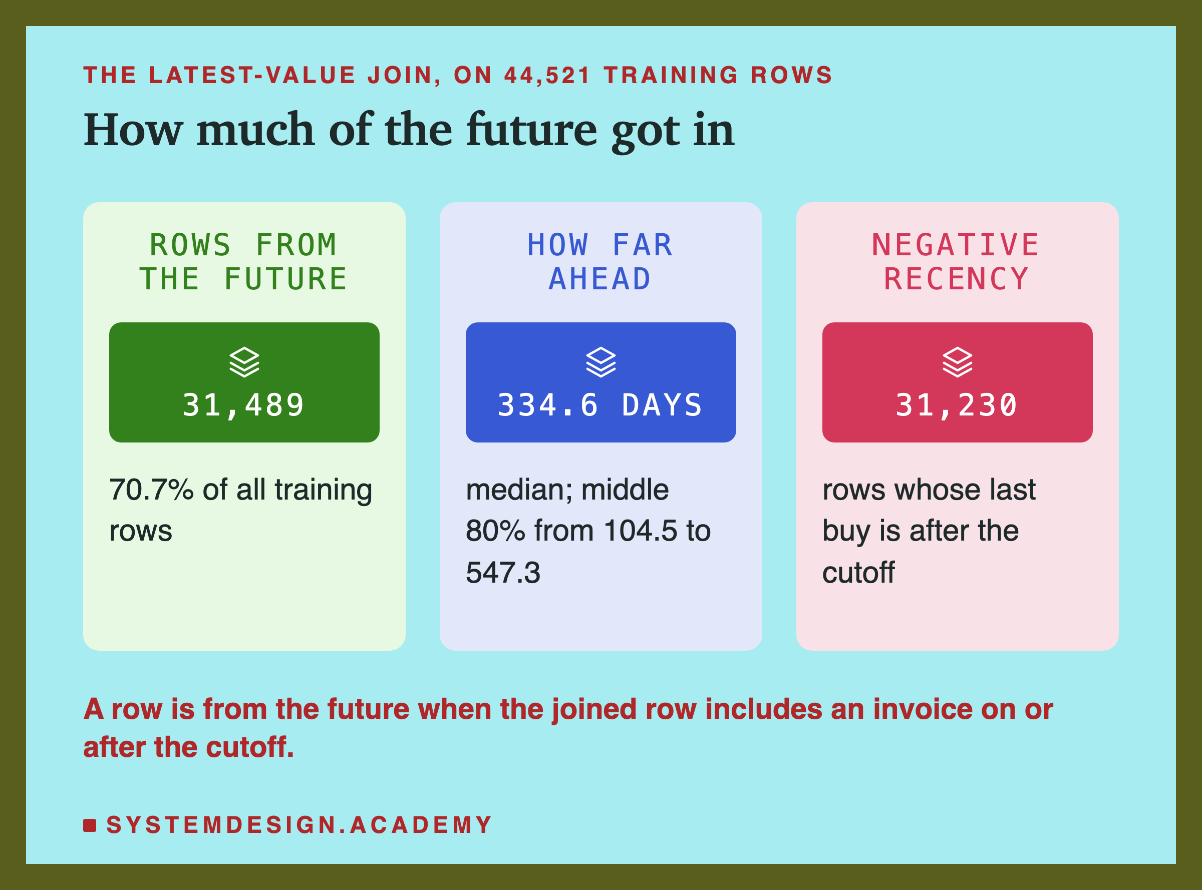
The lab counted the leak directly. A training row reads the future when the row joined to it includes any invoice on or after the cutoff.
With the latest-value join, 31,489 of the 44,521 training rows read the future: 70.7 percent. The median row looked 334.6 days ahead, nearly a year. The middle 80 percent of them looked between 104.5 and 547.3 days ahead.
31,230 rows had a negative recency, a last buy after the cutoff. A careful person might spot negative numbers and stop. But the other columns leak too, with nothing strange in them. A frequency of 8 instead of 1 is a perfectly normal-looking number.
Only 13,032 rows read nothing from the future. Those are customers who never made another invoice after the cutoff, so their latest row is also their point-in-time row.
Why the Latest Row Is Such a Strong Hint
Why does this leak help so much offline? The counts answer it.
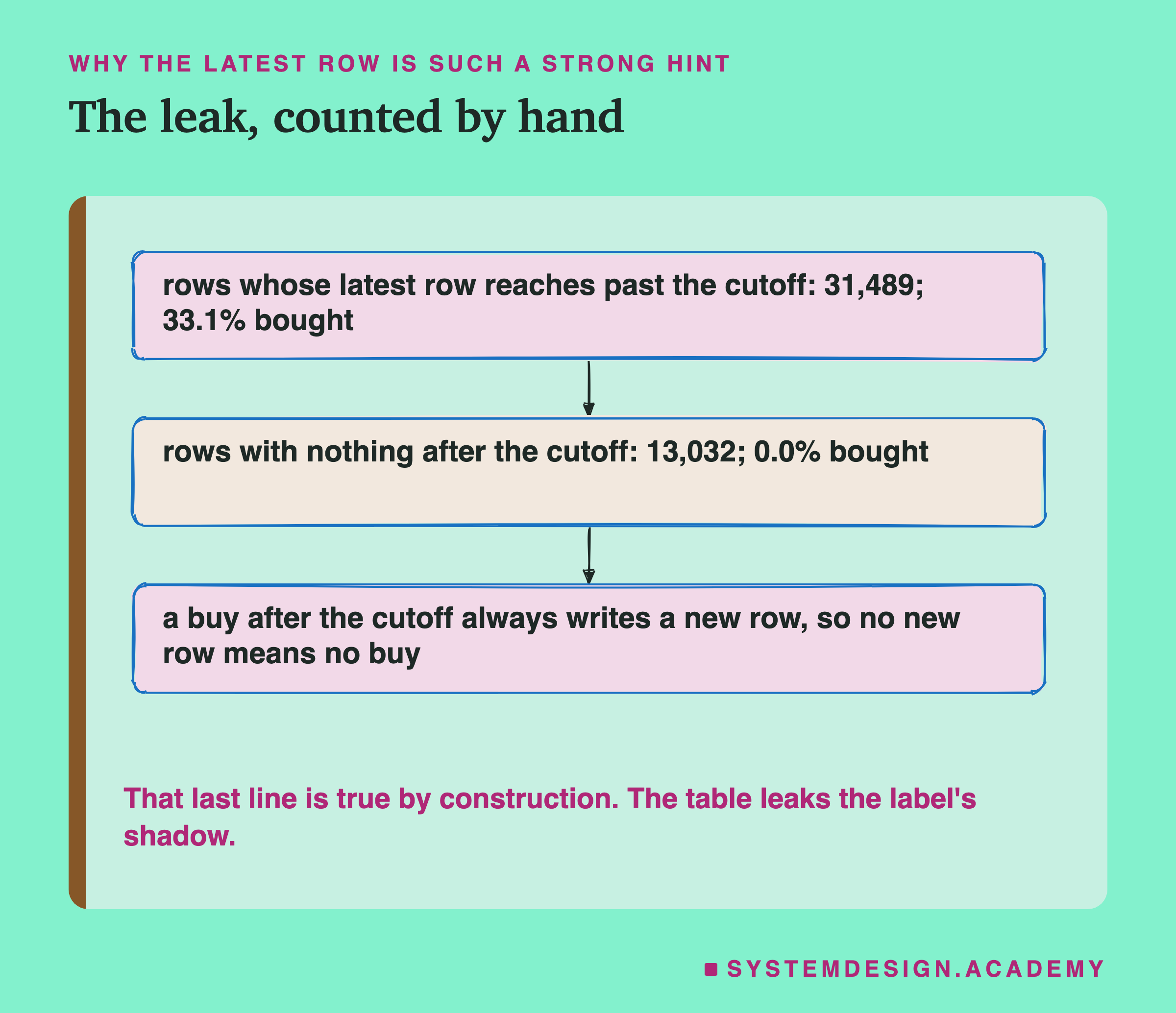
Of the rows whose latest row reaches past the cutoff, 33.1 percent bought in the 30-day window. Of the rows with nothing after the cutoff, 0.0 percent bought.
That zero is not a finding. It is true by construction. If a customer buys in the window, that buy writes a new row after the cutoff, so their latest row must reach past it. A row with nothing after the cutoff therefore cannot be a buyer. The latest-value table splits the rows into "certainly did not buy" and "might have bought" before the model learns anything.
On top of that, the latest row carries the buy itself: its frequency is higher, its money is higher and its recency is negative. The model does not need to learn anything about customers. It only needs to notice which rows carry traces of the window it is meant to predict.
Is the End-of-Data Table an Unfair Example?
A fair objection: no team trains in 2011 on a table that runs to the end of 2011. The latest row in my table is often a year after the cutoff, because the data ends in December 2011. A real team builds its training set on some day, from the table as it is that day. So, after a review, I measured two more realistic teams. This slide was added after the first results.
The first team builds right after the training months, from the table as it stood on 1 April 2011. The second builds on 1 July 2011, just before the test months. Each takes every customer's newest row in the table on that day and joins it to every training row.
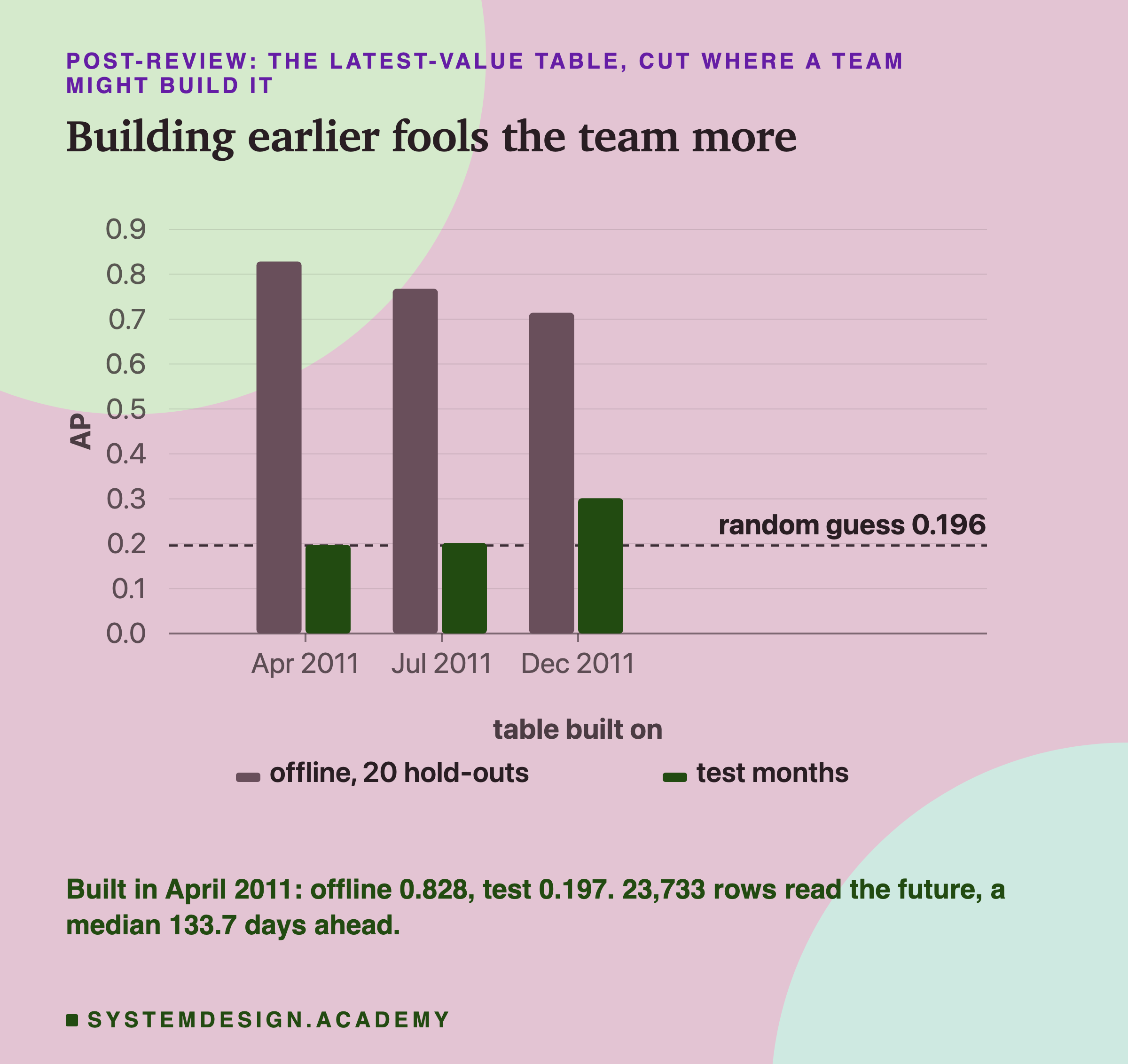
| table built on | rows from the future | median days ahead | offline AP | test AP |
|---|---|---|---|---|
| 1 April 2011 | 23,733 | 133.7 | 0.828 | 0.197 |
| 1 July 2011 | 27,604 | 187.6 | 0.767 | 0.201 |
Which Column Carries the Leak?
The design asked one more question before the run: which of the four columns carries the leak? For each column, the lab built a training table with that one column from the latest row and the other three point-in-time.
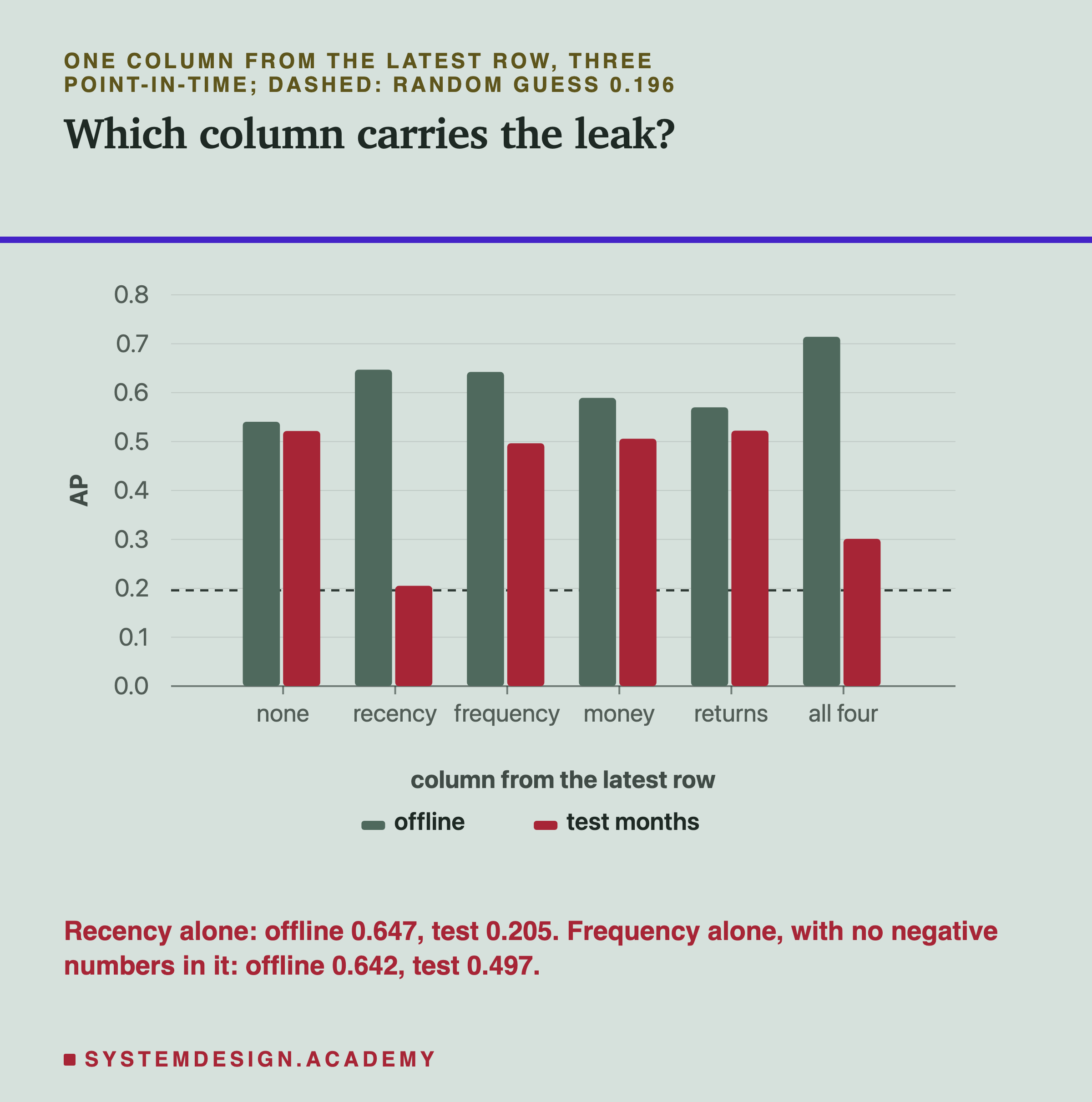
| column from the latest row | offline AP | test AP |
|---|---|---|
| none (point-in-time) | 0.540 | 0.522 |
| recency | 0.647 | 0.205 |
| frequency | 0.642 | 0.497 |
| money | 0.589 | 0.506 |
| return share | 0.570 | 0.522 |
| all four | 0.714 |
Off by One Day
The latest-value join is a big, obvious mistake once you know to look for it. The next one is small and easy to miss.
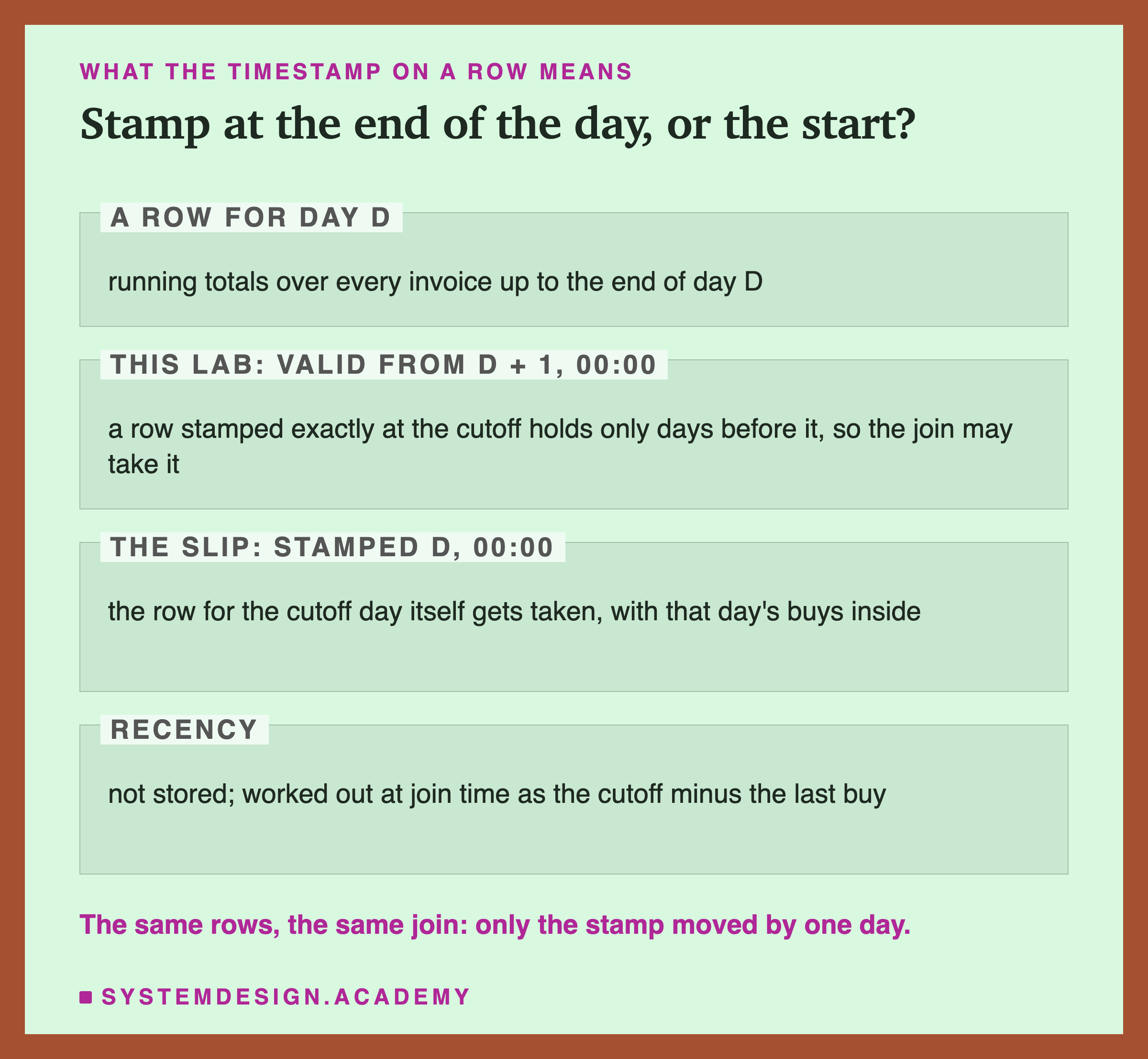
Many tables are split by date, one part per day. It is natural to stamp a day's row with that day's date, which means midnight at the start of the day. But the row holds totals up to the end of the day. If you then join "at or before the cutoff", the row for the cutoff day itself gets matched, and it holds that day's buys. Those buys are inside the label window.
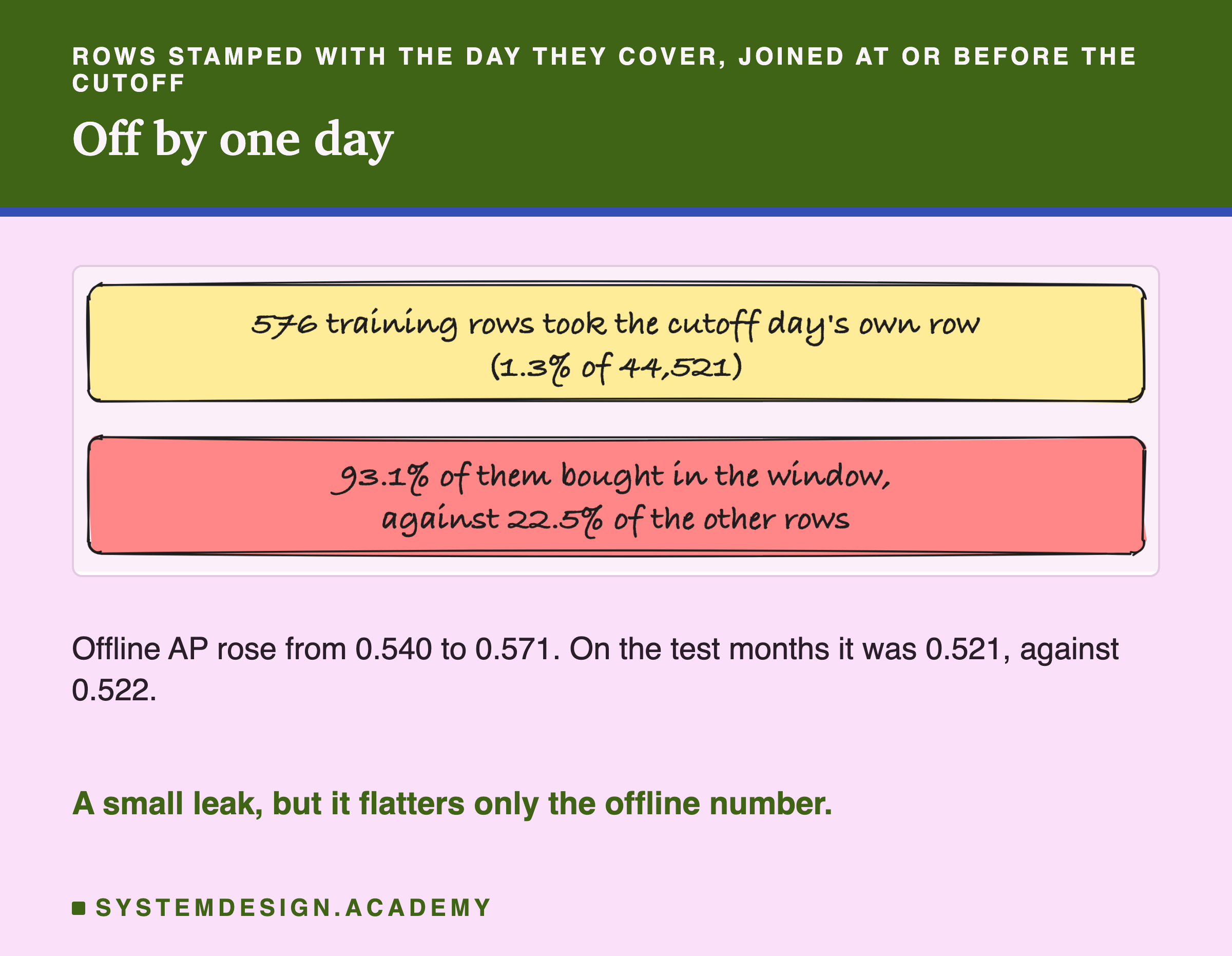
The lab measured it rather than assuming it. Stamping at the start of the day let 576 training rows, 1.3 percent, take the cutoff day's own row. Of those rows, 93.1 percent bought in the window, against 22.5 percent of the rest. Of course they did: many of them were buying that very day.
The offline AP, per cutoff, rose from 0.540 to 0.571, and it was higher in all 20 seeds. On the test months the score was 0.521, against 0.522 for the correct table. So this slip did not hurt the real model much here. It only made the offline number lie by about 0.031. Take a different task, such as predicting a buy in the next day instead of the next 30. Then the cutoff day would be most of the window, and the same slip could matter far more. I did not test that.
allow_exact_matches: True or False?
pd.merge_asof has a setting called allow_exact_matches. With True, its default, it may take a row stamped exactly at the cutoff. With False, only rows stamped strictly before it. Which one is right depends on what your stamp means, so I chose it on purpose.
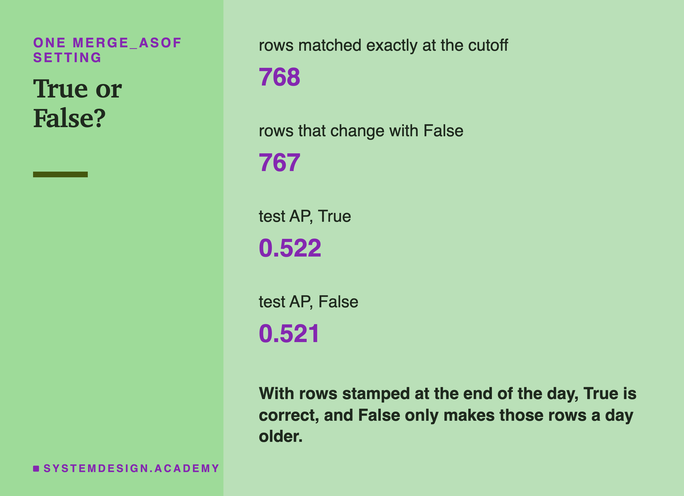
In this lab a row is stamped at midnight after the day it covers. A row stamped exactly at the cutoff therefore covers the day before the cutoff, and holds nothing from the cutoff onward. It is legal, and it is the freshest legal row. So True is correct here.
I also ran False, as a check on that reasoning. 768 training rows had a row stamped exactly at their cutoff: customers with an invoice on the last day of the month. With False, 767 of them took an older row instead. The test AP went from 0.522 to 0.521. Nothing leaks either way; False only throws away one day of freshness.
The one row that did not change belongs to a customer who, so far, had only returned things, so the older row held the same values. I found that after the results, in the report script.
The general rule: if your stamp means "valid from", use True. If your stamp is the time of the event itself, and a feature row stamped exactly at the cutoff could hold an event at the cutoff, use False. If you do not know which your stamp means, find out before you train. If you cannot find out, use False. With daily rows like these, it costs at most a day of freshness, while True can leak. With weekly or hourly rows, the cost is one row's period, a week or an hour.
The Joins in the Lab's Code
The lab is one Python file, scripts/labs/features/point_in_time.py. Four functions carry the whole lesson.
feature_table is the nightly job. It groups the invoices by customer and day, adds up each day, then keeps running totals with cumsum, which adds each day to all the days before it. It stamps each row with the next midnight. One line carries the time of the last buy forward with ffill, which fills a gap with the value above it. My first run was missing that line.
join_pit is the point-in-time join, one call to pd.merge_asof. It sorts the training rows by cutoff and the table by stamp, because merge_asof needs both sorted by the time it matches on. It matches by customer, with direction="backward", which means "the newest row at or before", and allow_exact_matches=True. Then it works out recency as the cutoff minus the last buy, in days.
join_latest is the mistake, written on purpose. It keeps each customer's newest row with groupby("customer_id").tail(1) and merges it onto every training row. It is shorter than the correct join, and it runs without any error.
brute_force is the check. For each cutoff, it takes only the invoices before it and counts everything again from scratch. It is slow and simple, which is the point: it is too simple to share a bug with the clever version.
Try It Yourself
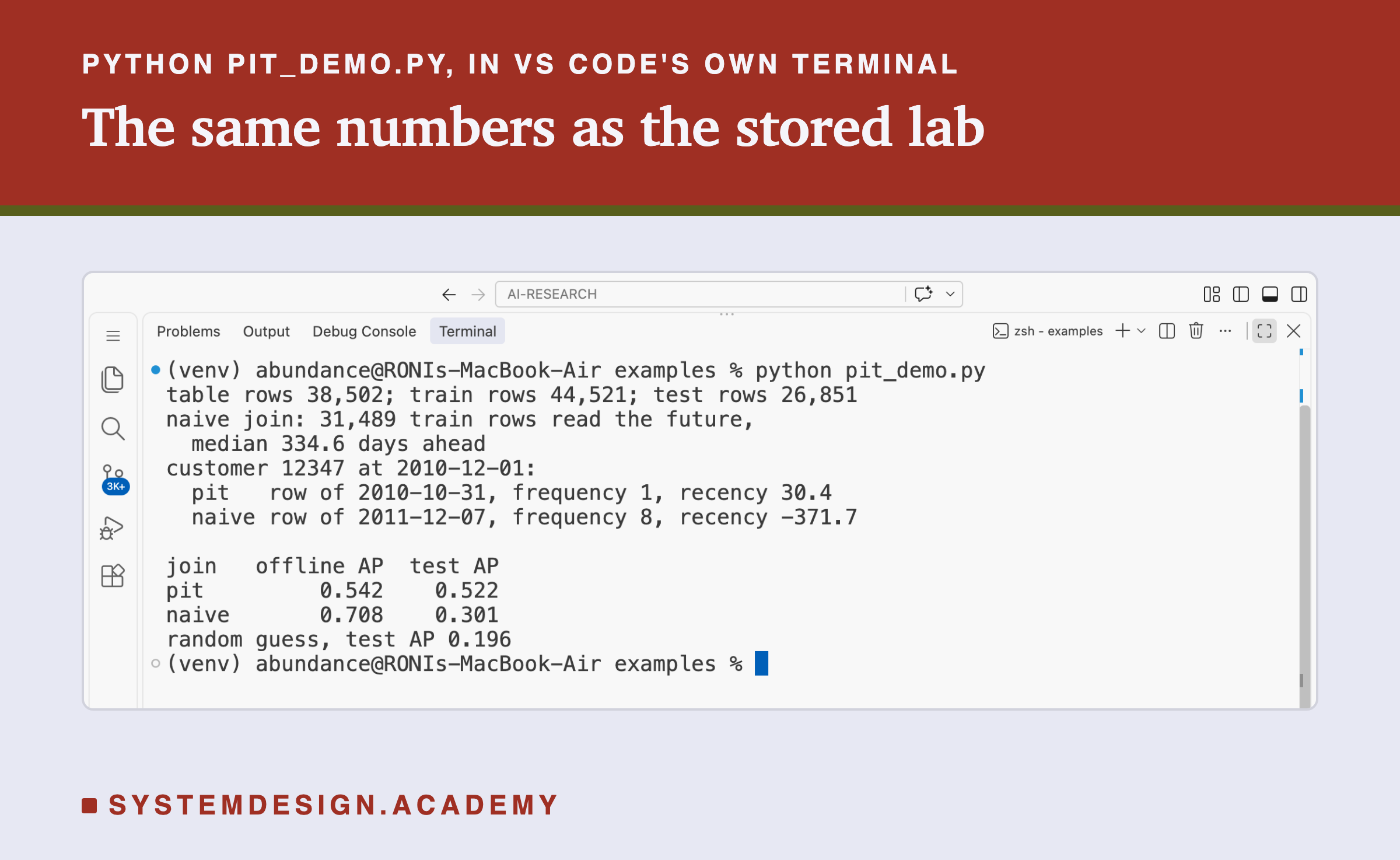
The full lab trains 211 models and took about seven and a half minutes on my laptop. I wrote a small demo that does the heart of it: the table, the two main joins, the leak count, customer 12347, and one hold-out per join.
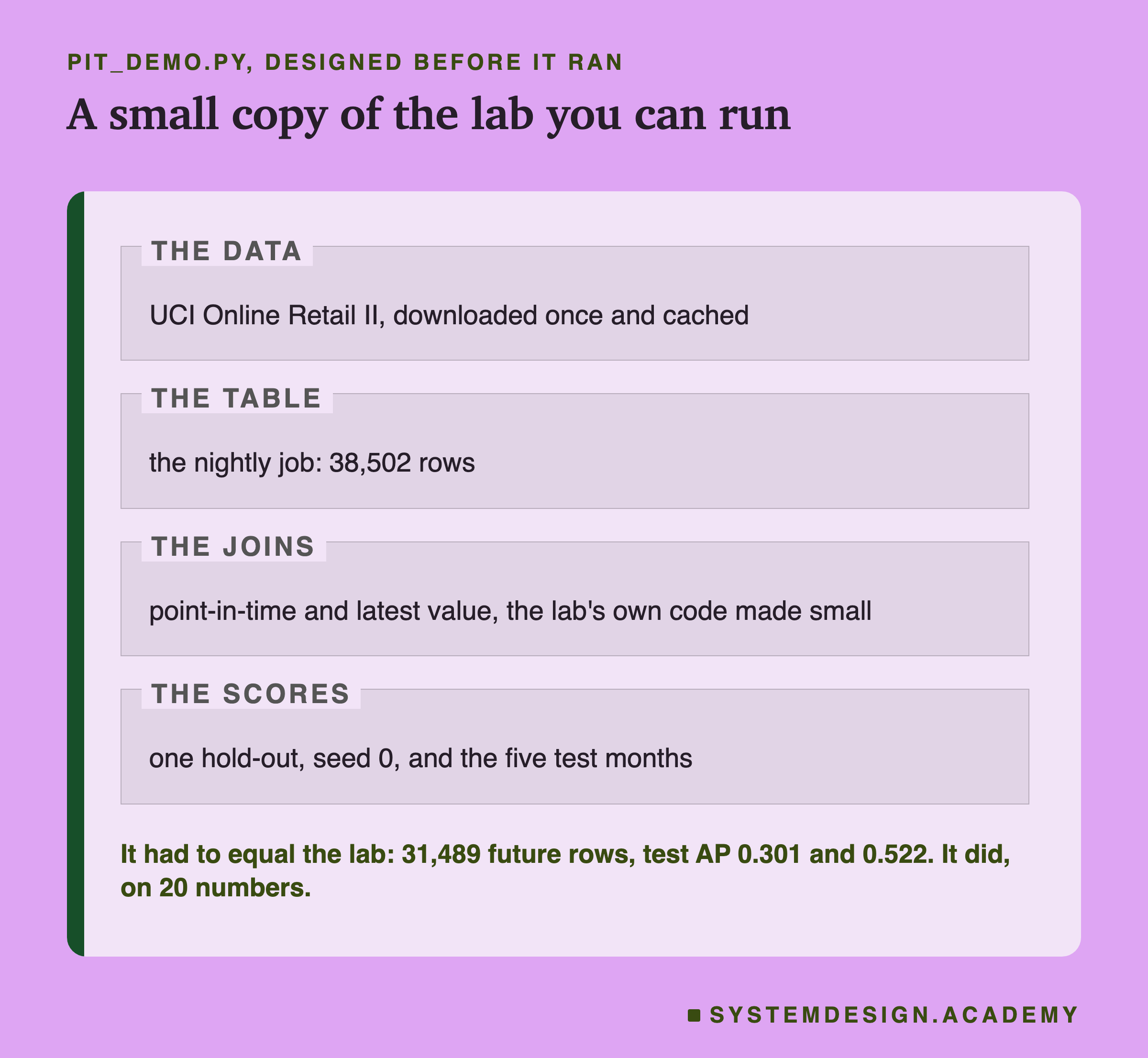
I wrote the demo's design into its docstring on 1 October 2026, after the lab had run and before the demo ran. The design names the numbers it must reproduce. To get the same hold-out rows as the lab, it keeps the training rows in the lab's order, because a seed picks row positions, not customers.
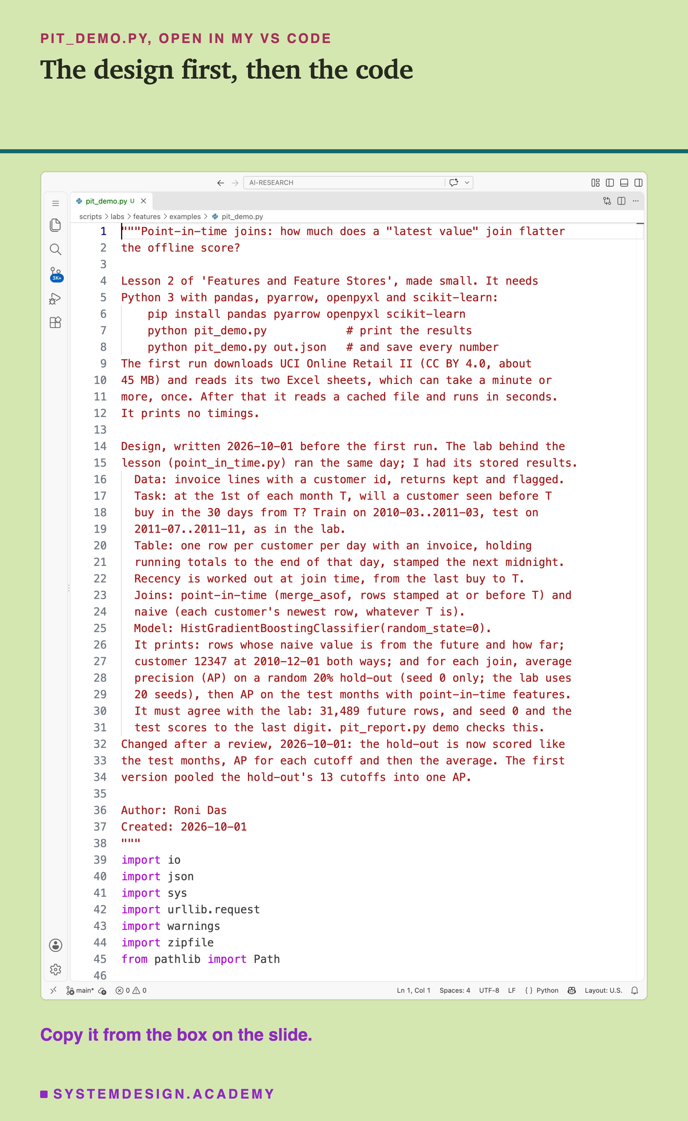
Before you run this lab. You need Python 3 and four libraries: pip install pandas pyarrow openpyxl scikit-learn. The first run downloads the dataset, about 45 MB, and reads its Excel sheets. On my Mac that first run took about a minute. Later runs read a cached file and take a few seconds. It needs no GPU, the graphics chip many machine learning jobs use. I ran it with scikit-learn 1.9.1 and pandas 3.0.6 on a Mac. These libraries run on Windows and Linux too, but I have not checked the numbers there. Give it a file name, python pit_demo.py out.json, and it also saves every number. That is how results/pit-demo.json was made.
"""Point-in-time joins: how much does a "latest value" join flatter
the offline score?

Lesson 2 of 'Features and Feature Stores', made small. It needs
Python 3 with pandas, pyarrow, openpyxl and scikit-learn:
    pip install pandas pyarrow openpyxl scikit-learn
    python pit_demo.py            # print the results
    python pit_demo.py out.json   # and save every number
The first run downloads UCI Online Retail II (CC BY 4.0, about
45 MB) and reads its two Excel sheets, which can take a minute or
more, once. After that it reads a cached file and runs in seconds.
It prints no timings.

Design, written 2026-10-01 before the first run. The lab behind the
lesson (point_in_time.py) ran the same day; I had its stored results.
  Data: invoice lines with a customer id, returns kept and flagged.
  Task: at the 1st of each month T, will a customer seen before T
  buy in the 30 days from T? Train on 2010-03..2011-03, test on
  2011-07..2011-11, as in the lab.
  Table: one row per customer per day with an invoice, holding
  running totals to the end of that day, stamped the next midnight.
  Recency is worked out at join time, from the last buy to T.
  Joins: point-in-time (merge_asof, rows stamped at or before T) and
  naive (each customer's newest row, whatever T is).
  Model: HistGradientBoostingClassifier(random_state=0).
  It prints: rows whose naive value is from the future and how far;
  customer 12347 at 2010-12-01 both ways; and for each join, average
  precision (AP) on a random 20% hold-out (seed 0 only; the lab uses
  20 seeds), then AP on the test months with point-in-time features.
  It must agree with the lab: 31,489 future rows, and seed 0 and the
  test scores to the last digit. pit_report.py demo checks this.
Changed after a review, 2026-10-01: the hold-out is now scored like
the test months, AP for each cutoff and then the average. The first
version pooled the hold-out's 13 cutoffs into one AP.

Author: Roni Das
Created: 2026-10-01
"""
import io
import json
import sys
import urllib.request
import warnings
import zipfile
from pathlib import Path

import pandas as pd
from sklearn.ensemble import HistGradientBoostingClassifier
from sklearn.metrics import average_precision_score as ap_score
from sklearn.metrics import roc_auc_score as auc_score
from sklearn.model_selection import train_test_split

warnings.filterwarnings("ignore")
URL = ("https://archive.ics.uci.edu/static/public/502/"
       "online+retail+ii.zip")
CACHE = Path.home() / "lab-data" / "features" / "retail.parquet"
COLS = ["recency_days", "frequency", "money", "return_share"]
DAY = pd.Timedelta(days=1)
TRAIN = pd.date_range("2010-03-01", "2011-03-01", freq="MS")
TEST = pd.date_range("2011-07-01", "2011-11-01", freq="MS")


def load():
    """Invoice lines with a customer id, sorted by time."""
    if not CACHE.exists():
        raw = urllib.request.urlopen(URL).read()
        z = zipfile.ZipFile(io.BytesIO(raw))
        x = [n for n in z.namelist() if n.endswith(".xlsx")][0]
        a, b = pd.read_excel(z.open(x), sheet_name=None).values()
        df = pd.concat([a[a["InvoiceDate"] < b["InvoiceDate"].min()],
                        b], ignore_index=True)
        df = df.rename(columns={"Customer ID": "customer_id",
                                "InvoiceDate": "ts",
                                "Invoice": "invoice"})
        df = df.dropna(subset=["customer_id"])
        df["customer_id"] = df["customer_id"].astype(int)
        df["invoice"] = df["invoice"].astype(str)
        df["is_return"] = df["invoice"].str.startswith("C")
        df["amount"] = df["Quantity"] * df["Price"]
        df = df.sort_values(["ts", "invoice"], kind="stable")
        CACHE.parent.mkdir(parents=True, exist_ok=True)
        df[["invoice", "ts", "customer_id", "is_return",
            "amount"]].to_parquet(CACHE, index=False)
    return pd.read_parquet(CACHE)


def labels(ev, cutoffs):
    """(customer, T) rows: seen before T; buys in [T, T + 30 days)?"""
    buys = ev[~ev["is_return"]]
    out = []
    for t in cutoffs:
        seen = ev.loc[ev["ts"] < t, "customer_id"].unique()
        win = buys[(buys["ts"] >= t) & (buys["ts"] < t + 30 * DAY)]
        df = pd.DataFrame({"customer_id": seen, "cutoff": t})
        df["label"] = df["customer_id"].isin(set(win["customer_id"]))
        out.append(df.astype({"label": int}))
    return pd.concat(out, ignore_index=True)


def feature_table(ev):
    """The nightly job: running totals per customer per active day."""
    inv = ev.groupby(["customer_id", "invoice"], sort=False).agg(
        ts=("ts", "min"), ret=("is_return", "first"),
        amount=("amount", "sum")).reset_index()
    inv["day"] = inv["ts"].dt.normalize()
    inv["buy"] = (~inv["ret"]).astype(int)
    inv["spent"] = inv["amount"].where(~inv["ret"], 0.0)
    inv["buy_ts"] = inv["ts"].where(~inv["ret"])
    d = inv.groupby(["customer_id", "day"]).agg(
        buys=("buy", "sum"), rets=("ret", "sum"),
        money=("spent", "sum"), last_buy=("buy_ts", "max"),
        last_ts=("ts", "max")).reset_index()
    g = d.groupby("customer_id")
    d["frequency"] = g["buys"].cumsum()
    d["money"] = g["money"].cumsum()
    n_all = d["frequency"] + g["rets"].cumsum()
    d["return_share"] = (n_all - d["frequency"]) / n_all
    d["last_buy_ts"] = g["last_buy"].cummax()
    d["last_buy_ts"] = d.groupby("customer_id")["last_buy_ts"].ffill()
    d["feature_ts"] = d["day"] + DAY      # valid from next midnight
    return d.drop(columns=["buys", "rets", "last_buy"])


def point_in_time(rows, table):
    m = pd.merge_asof(rows.sort_values("cutoff", kind="stable"),
                      table.sort_values("feature_ts"),
                      left_on="cutoff", right_on="feature_ts",
                      by="customer_id", direction="backward",
                      allow_exact_matches=True)
    return recency(m)


def latest(rows, table):
    newest = table.sort_values("feature_ts").groupby(
        "customer_id").tail(1)
    return recency(rows.merge(newest, on="customer_id", how="left"))


def recency(df):
    df["recency_days"] = (df["cutoff"] - df["last_buy_ts"]) / DAY
    return df          # rows stay in the order labels() made them


def model():
    return HistGradientBoostingClassifier(random_state=0)


def scores(y, p):
    return {"ap": float(ap_score(y, p)), "auc": float(auc_score(y, p))}


def by_cutoff(df, m):
    """AP and ROC-AUC for each cutoff, then the average."""
    per = [scores(g["label"], m.predict_proba(g[COLS])[:, 1])
           for _, g in df.groupby("cutoff")]
    return {k: sum(s[k] for s in per) / len(per) for k in ("ap", "auc")}


ev = load()
table = feature_table(ev)
train_rows, test_rows = labels(ev, TRAIN), labels(ev, TEST)
train = {"pit": point_in_time(train_rows, table),
         "naive": latest(train_rows, table)}
test = point_in_time(test_rows, table)

nv = train["naive"]
future = nv["last_ts"] >= nv["cutoff"]
ahead = ((nv["last_ts"] - nv["cutoff"]) / DAY)[future]
print(f"table rows {len(table):,}; train rows {len(nv):,}; "
      f"test rows {len(test):,}")
print(f"naive join: {future.sum():,} train rows read the future,")
print(f"  median {ahead.median():.1f} days ahead")

T = pd.Timestamp("2010-12-01")
print(f"customer 12347 at {T.date()}:")
ex = {}
for kind, df in train.items():
    r = df[(df["customer_id"] == 12347) & (df["cutoff"] == T)].iloc[0]
    ex[kind] = {"frequency": int(r["frequency"]),
                "money": round(float(r["money"]), 2),
                "recency_days": float(r["recency_days"])}
    print(f"  {kind:5s} row of {r['day'].date()}, frequency "
          f"{r['frequency']}, recency {r['recency_days']:.1f}")

print(f"\n{'join':6s} {'offline AP':>10s} {'test AP':>8s}")
offline, served = {}, {}
for kind, df in train.items():
    a, b = train_test_split(df, test_size=0.2, random_state=0)
    m = model().fit(a[COLS], a["label"])
    pooled = scores(b["label"], m.predict_proba(b[COLS])[:, 1])
    offline[kind] = {**by_cutoff(b, m), "ap_pooled": pooled["ap"]}
    m = model().fit(df[COLS], df["label"])
    served[kind] = by_cutoff(test, m)
    print(f"{kind:6s} {offline[kind]['ap']:10.3f} "
          f"{served[kind]['ap']:8.3f}")
guess = test.groupby("cutoff")["label"].mean().mean()
print(f"random guess, test AP {guess:.3f}")

if len(sys.argv) > 1:
    out = {"rows": {"train": len(nv), "test": len(test)},
           "table_rows": len(table), "future_rows": int(future.sum()),
           "days_ahead_median": float(ahead.median()),
           "example": {"customer_id": 12347, **ex},
           "offline_seed0": offline, "test": served}
    json.dump(out, open(sys.argv[1], "w"), indent=1)
Do the As-Of Join by Hand
This box holds customer 12347's real feature table, exactly as the nightly job wrote it. It needs nothing but Python, so it runs in your browser. Press Run to see what each join gives at the cutoff 1 December 2010.
Then change CUTOFF to another first of the month, such as "2011-05-01", and run again. Watch which row each join takes. Last, set CUTOFF = "2010-11-01" and EXACT = False. The customer's first row is stamped exactly at that cutoff. With False there is no row stamped strictly before the cutoff, so the join returns empty features.
The report script writes this box from the stored lab results. It then runs the box at all 21 cutoffs, once with EXACT = True and once with False. Each answer must match the lab's own merge_asof for this customer.
Common Mistakes, and When Each Check Helps
Joining the current values onto old rows. This is the latest-value join. It often hides inside a helper that "gets the customer's features", written for the live system and reused for training. The live system should read the latest values. Training rows must not.
Storing only the latest value. If your feature table overwrites old values, you cannot build a point-in-time training set at all, however careful the join. Keep every version with the time it became true.
Not knowing what the stamp means. A stamp can mean when the event happened, when the job ran, or the start of the day the row covers. The off-by-one slip came from that alone. Write down what your stamp means, next to the table.
Storing values that change by themselves. Recency changes every day. A stored recency is stale the day after it is written. Store the time of the event and work out the age at join time.
Trusting a random hold-out to catch a leak. It cannot. All twenty hold-outs here came from the same leaky table and all twenty agreed with each other, because each was cut from that table. Only scoring later months, with features built the way serving builds them, showed the truth. Later months alone are not enough. When their features were also joined latest-value, the leaky model got an AP of 0.822 on them. I measured that after the review.
When a point-in-time join matters. Whenever a training row stands for a past moment and features change over time: almost every prediction about customers, users, machines or prices.
When it does not. When features never change after they are first known, like a customer's country of signup. Or when every training row was built and stored at the moment it happened. Even then, check a few rows against the raw events.
What This Lab Cannot Tell You
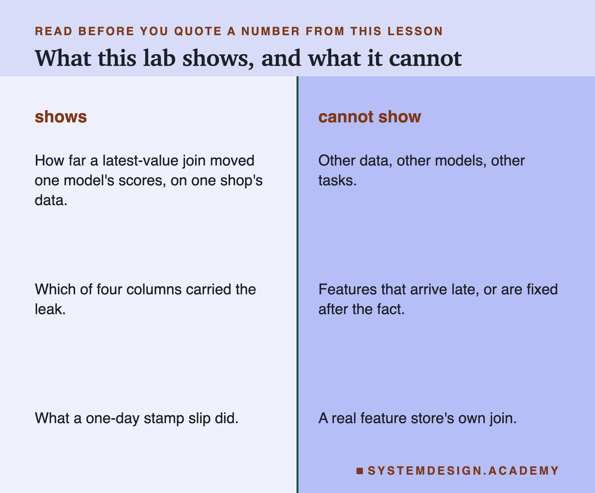
One shop, one task, one model. The sizes here belong to this data, a 30-day window and this model. A different task could leak more or less. A leaky table always looked better offline here. Whether it did worse later depended on the column: return share alone looked better offline, 0.570 against 0.540, and scored the same on the test months, 0.522. The numbers do not travel to other data.
Three build dates. I measured latest-value tables built at three dates: April 2011, July 2011 and December 2011. A team building on another date, or refreshing its training set every month, could see different numbers.
Clean arrival times. Every invoice here arrives in the table the same night. In real pipelines some data arrives late, or gets corrected later. A row stamped by when it arrived and a row stamped by when it happened can disagree. A later lesson in this chapter simulates late data.
One seed for the model. The model always used random_state=0. The 20 seeds vary the hold-out, not the model's own randomness, which here mainly sets the 10 percent it keeps aside for early stopping.
No real . I wrote the join by hand in pandas. Whether a product does the same thing is a question for its own test, which the last lesson of this chapter runs.
What to Do on Monday
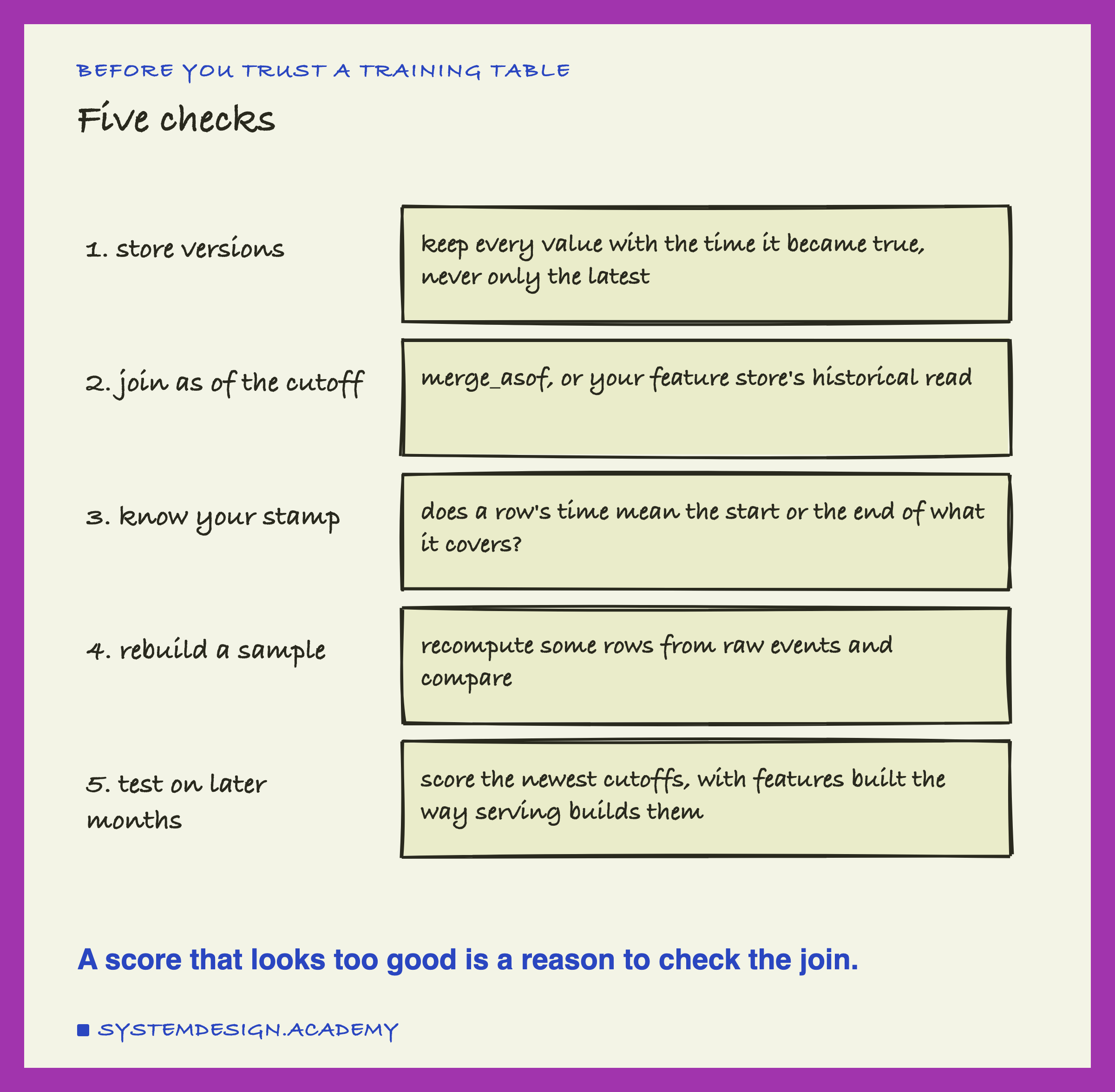
These are the five checks I would make before trusting any training table built from a feature table.
-
Store versions. Every value, with the time it became true. Never overwrite.
-
Join as of the cutoff. In pandas,
merge_asofby entity, backward in time. An entity is the thing a feature describes, here a customer. In a , use its historical read, never its live read, the call that returns today's values for serving. -
Know your stamp. Decide whether a row's time is the start or the end of what it covers, and set
allow_exact_matchesto match. If you cannot find out what the stamp means, use False. With daily rows like these, it costs at most a day of freshness, while True can leak. With weekly or hourly rows, the cost is one row's period. -
Rebuild a sample. Take a few hundred training rows and recompute their features from the raw events, using only events before each cutoff. Any difference is a bug. Mine was found exactly this way.
-
Test on later months. Keep the newest cutoffs aside, build their features the way the live system will, and score them once at the end. A random hold-out cut from a leaky table leaks too, and so do later months joined the same leaky way: there the leaky model scored 0.822.
Knowledge Check
Knowledge Check
4 questions - Score 80% to pass
A team joins each customer's current feature values onto training rows from last year. What did this lab find?
Why did twenty different random hold-outs all fail to reveal the leak?
Rows are stamped at midnight after the day they cover. Which merge_asof setting is right, and why?
In the latest-value table, 0.0 percent of the rows with nothing after the cutoff were buyers. Why?