The Model That Passed Every Test and Failed in Production
A team ships a fraud model. Offline, on the held-out test set, it looks incredible: high precision, high recall, a clean ROC curve, everyone signs off. It goes live. Within two weeks the fraud operations team is furious, because the model is missing obvious fraud and flagging good customers at the same time. Nothing crashed. No exception was thrown. No alert fired. The model is just quietly, confidently wrong, and the offline metrics that everyone trusted still look perfect when you re-run them.
Someone finally traces it. One of the model's inputs is "the user's average transaction amount over the last 30 days." In the training notebook, a data scientist computed that with a tidy pandas line over the historical warehouse table: a rolling 30-day mean, keeping cents. In the production service, a backend engineer reimplemented the same idea in Java, rounded to whole currency units for a display concern that leaked into the feature, and used a fixed 30-day window that started at midnight instead of a true rolling 30 days. Small differences, each one defensible in isolation. Together they mean the model was trained on one definition of that feature and served a subtly different one on every single request.
That is train and serve skew, and it is the single most common way machine learning quietly breaks in production. The feature the model sees during training is not the feature it sees at request time, so every prediction is nudged off in a way the model was never taught to correct for. It is brutal to catch precisely because nothing looks broken. There is no stack trace to grep, no failing test to bisect. Accuracy just leaks away, and by the time anyone connects the business decline to a rounding rule, weeks have passed.
The model was never wrong. It was fed one version of the truth in training and a different version in production. Same name, different number.
A exists to make that specific bug structurally impossible, and to solve three related problems in the same stroke: keeping training and serving in sync, building leak-free training data, and letting teams reuse features instead of rebuilding them. This lesson is about how each of those falls out of one idea.
What a Feature Store Actually Is
A is the single source of truth for features. Instead of every notebook and every service computing features on their own, the feature logic is defined once, in one place, and everyone reads from it by name. That sounds almost too simple to matter, but the entire value of the system comes from refusing to let a feature be computed in two places.
Three ideas make it work, and they are worth naming precisely because the rest of the lesson is just consequences of them:
- One definition. A feature like
user_7d_order_countis written once, as code, with an owner. Both training and serving get their values from that one definition, so they cannot drift apart. Nobody reimplements it in another language for another runtime. - Two stores, on purpose. The same feature is materialized into two different places tuned for two different jobs: a big, cheap offline store for building training sets over full history, and a fast online store for serving live predictions by key. This is the counterintuitive part, and the next few slides are devoted to why one store cannot do both jobs.
- A registry in the middle. A catalog knows what each feature means: its data type, which entity it belongs to (a user, a driver, a merchant), where its values live, who owns it, and how fresh it is. Training and serving both ask this registry for features by name rather than by hand-written query.
Here is the whole thing on one canvas. Raw data comes in, one pipeline computes each feature exactly once, the registry catalogs it, and the result fans out to the two stores that training and serving read from.
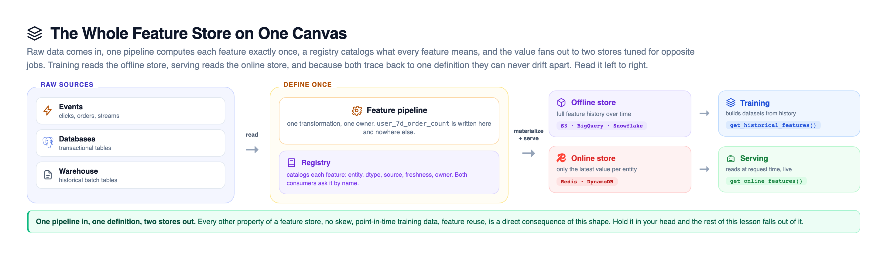
The shape to remember is one pipeline in, one definition, two stores out. Every other property in this lesson, the absence of skew, correct point-in-time training data, and feature reuse across teams, is a direct consequence of that shape. Hold it in your head and the rest of the lesson falls out of it.
The Bug It Exists to Kill, Drawn Out
Before the mechanics, look at the failure and the fix side by side, because the whole design decision makes sense only against the bug it prevents. On the left is how skew happens when there is no single source of truth. On the right is why one definition makes it impossible.
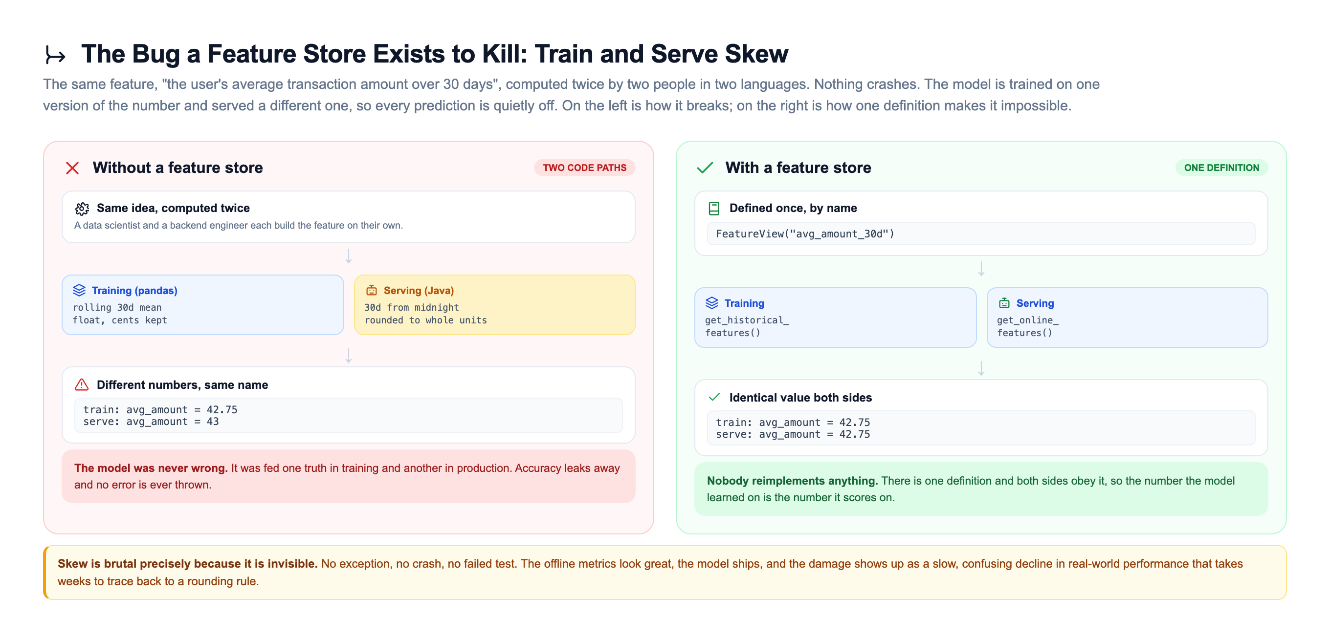
The left panel is the fraud story from the first slide, generalized. Two competent engineers, two runtimes, two slightly different implementations of one feature, and the model is silently trained on one and served the other. The right panel is the entire fix: there is exactly one definition, and both training and serving are thin clients that read from it. Nobody reimplements anything, so there is nothing to drift.
What makes skew so dangerous is that it is invisible by construction. A schema change throws an error. A null where a number is expected throws an error. But a feature that is off by a rounding rule or a window boundary is a perfectly valid number that happens to be wrong, so it sails through every type check and range check you have. The offline evaluation, which reads the training-side feature, looks flawless, because the training-side feature is internally consistent with itself. The gap only exists between training and serving, and no offline test ever crosses that boundary. That is why skew has to be prevented by architecture rather than caught by a test.
Two Stores, Because Training and Serving Want Opposite Things
Why keep the same feature in two places at all? Because training and serving have completely different access patterns, and no single database is good at both.
Training wants to scan enormous history. To build a dataset you might join labels to features across two years and a billion rows, computing aggregates over huge time ranges. You do not care if that query takes three minutes, because it runs once, offline, in a pipeline. What you care about is that it is cheap per terabyte and can chew through vast ranges without falling over. That is a columnar file format like Parquet on object storage, or a warehouse table in BigQuery or Snowflake, engineered for scan .
Serving wants one number, right now. When a live request arrives, you need this specific user's current features in a few milliseconds, because that read sits inside the request the customer is waiting on. You do not want two years of history and you cannot afford a full scan. You want the single latest value, looked up by key, instantly, tens of thousands of times per second. That is a key-value store like or DynamoDB, engineered for point reads and QPS.
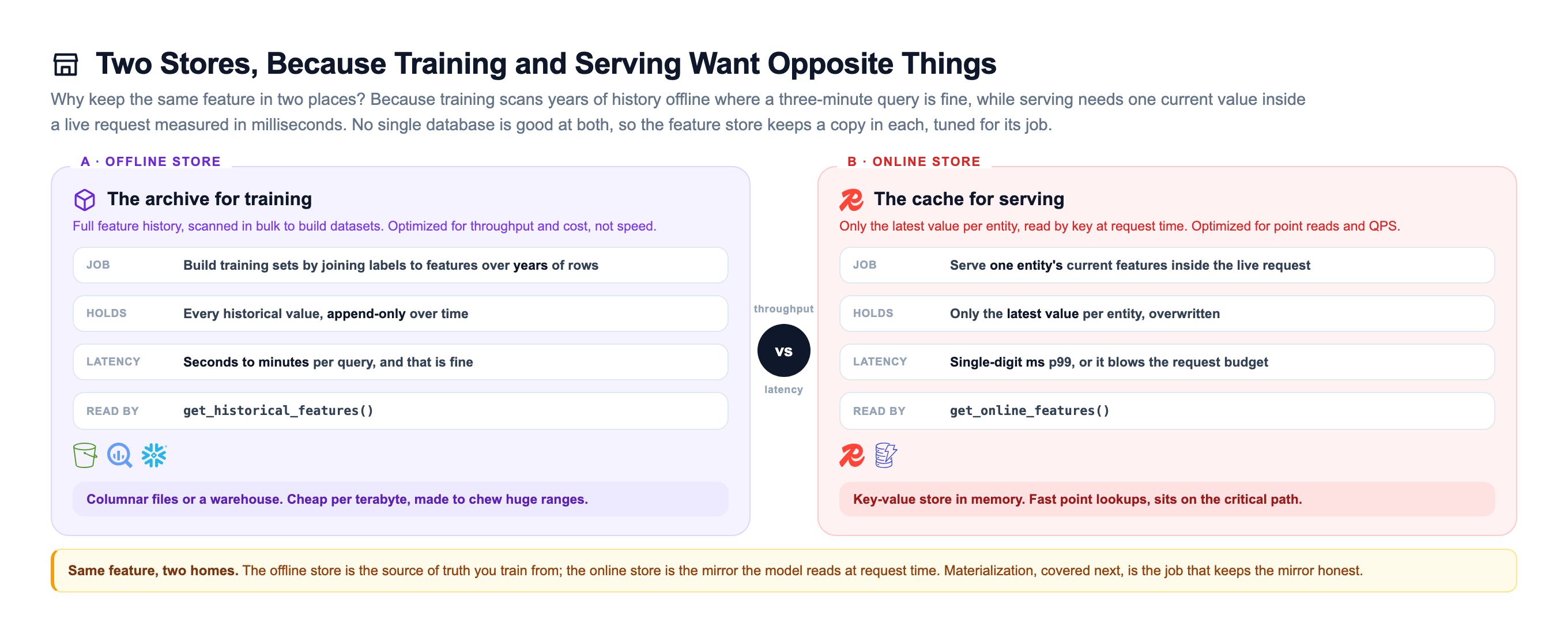
Same feature, two homes tuned for opposite jobs. The offline store is the archive you train from and the source of truth. The online store is the mirror the model reads at request time. The obvious next question is how the mirror stays faithful to the archive, and that is a job called materialization, two slides ahead. First, look at how these two stores keep training and serving reading the same truth.
An Online Read, Inside the Request Budget
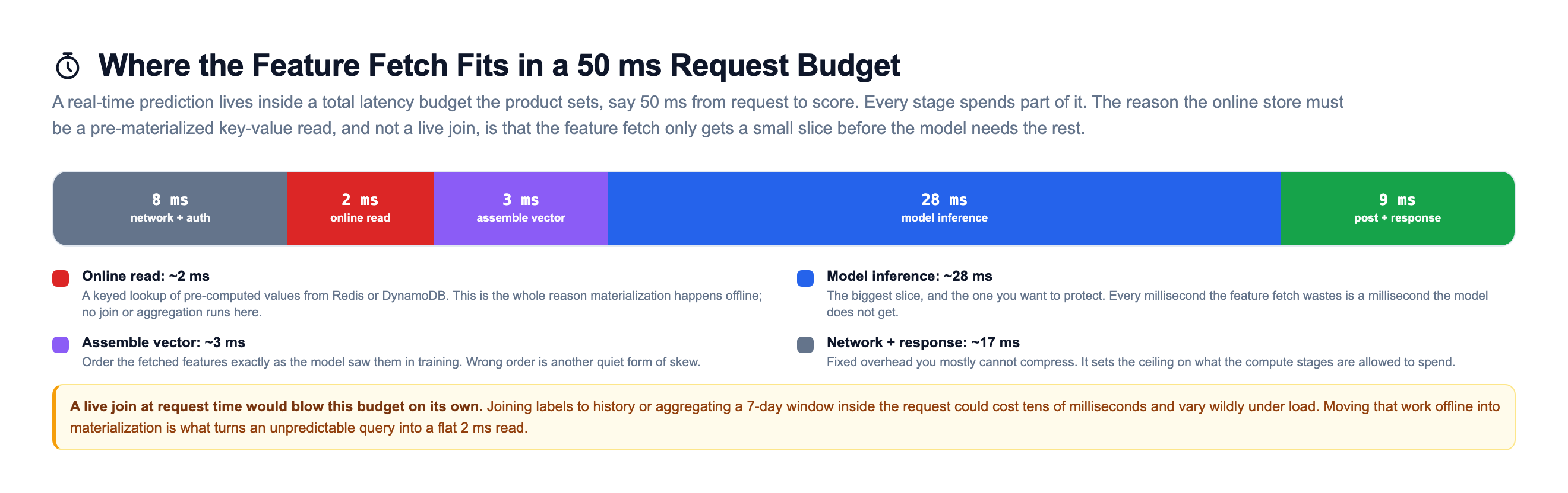
The reason the online store has to be a boring key-value lookup, and not a live query, is . A real-time prediction lives inside a hard budget the product sets, often something like 50 milliseconds from request to score. The feature fetch is not the whole request; it is one hop on the critical path, and it has to be fast enough to leave room for the model itself.
Trace exactly what happens when a request arrives. The serving API asks the SDK for a named set of features, the SDK resolves those names through the registry and issues one keyed read against the online store, and the store returns the pre-computed latest values. There is no join, no aggregation, no history walked at request time, because all of that already happened offline.
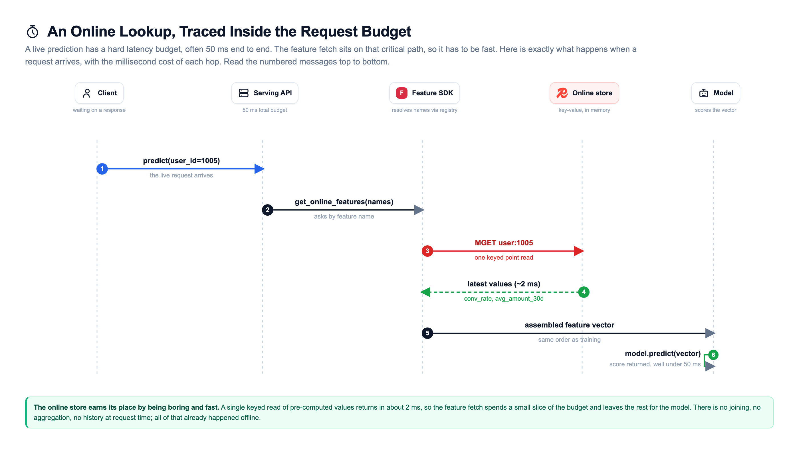
The single keyed read of pre-computed values returns in around two milliseconds, so the feature fetch spends a small slice of the budget and leaves the rest for inference. This is the whole reason the heavy work is pushed offline: a live join or a live aggregation inside the request could cost tens of milliseconds and, worse, vary wildly under load, blowing the budget exactly when traffic is highest. Notice too that the SDK assembles the vector in the same order the model saw during training. Getting that order wrong is another quiet form of skew, and the store is the natural place to guarantee it.
Materialization: Keeping the Mirror Honest
The two stores stay in sync through a scheduled job called materialization. The offline store fills up continuously as the feature pipeline writes history. Serving cannot scan that history live, so on a schedule the copies the latest value per entity out of the offline store and upserts it into the online store by key.
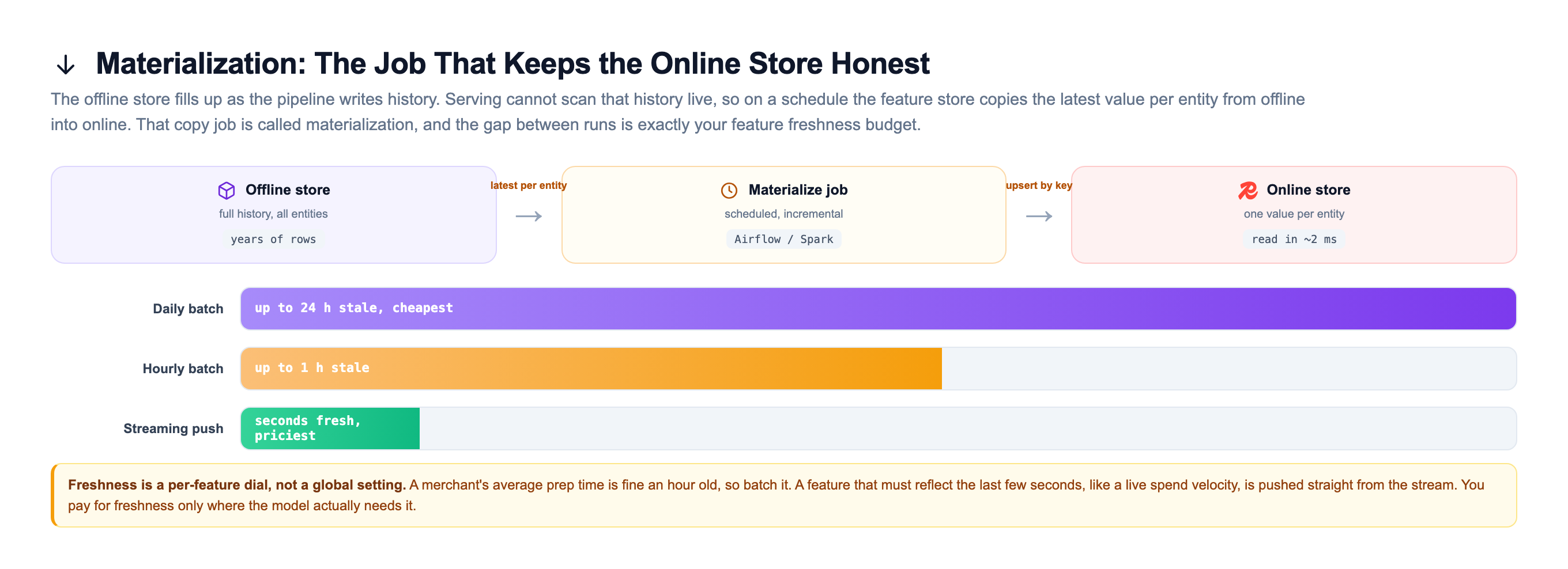
The gap between materialization runs is your feature freshness budget, and it is the single most important operational knob in the system. Materialize once a day and an online value can be up to 24 hours old, which is completely fine for a slow-moving trait like a user's home city or lifetime order count. Materialize hourly and you bound staleness to an hour, which suits aggregates that drift over a day. For a feature that must reflect the last few seconds, batch is not enough at all; you push updates directly from a stream into the online store as events arrive.
Freshness is not free, and that is the point. A streaming feature needs always-on infrastructure and careful state management, so it costs far more to build and run than a nightly batch job. The discipline is to set freshness per feature, at the cheapest setting that still keeps the model's decision correct. You are buying freshness, and you should only buy it where the prediction actually depends on it.
Point-in-Time Correctness: The Bug That Fools Everyone
There is a second, sneakier form of skew, and it lives entirely in how you build the training set. It is called label leakage, and a good is what saves you from it. This one fools even careful teams, because it produces training data that looks not just valid but excellent.
To train, you join features to labeled events. Say you are predicting fraud on a transaction that happened at 10:05 AM. Which value of "the user's 7-day order count" do you attach to that row? The value that was true at 10:05, or the value that is true now, hours later, after more orders came in? If you grab the current value, you have just leaked the future into the past. The model learns from information that did not exist at prediction time, and it will never have that information in production either.
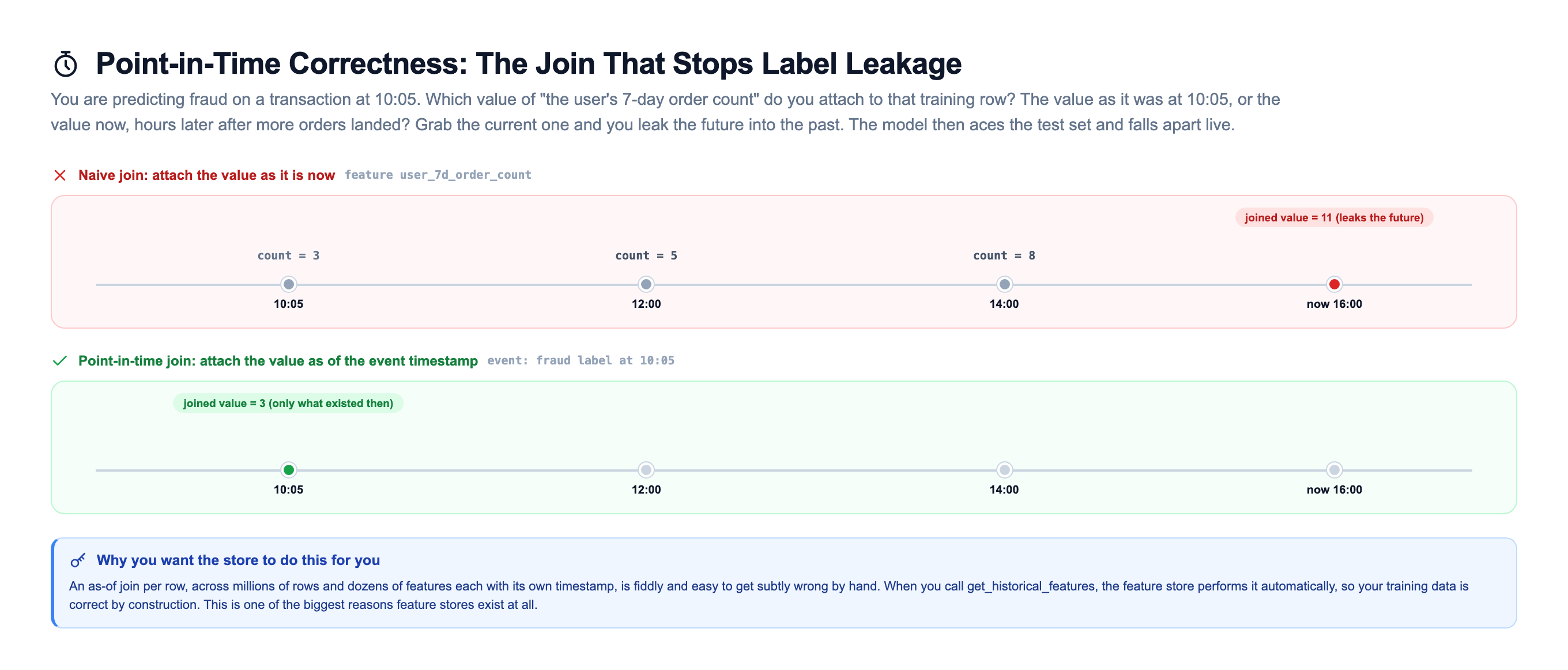
The fix is a point-in-time join, sometimes called an as-of join: each training row sees only the feature values that existed at that event's own timestamp, and nothing later. Done right, it makes training data correct by construction, so the distribution the model learns matches the distribution it will actually be scored against. Done by hand, it is fiddly and error-prone, especially across millions of rows and dozens of features that each carry their own timestamp and update on their own cadence. This is exactly why you want the feature store to do it for you. When you call get_historical_features, the store performs the as-of join per row automatically. Correct-by-construction training data is one of the biggest reasons feature stores exist at all, and the one hardest to replicate with a pile of ad hoc scripts.
Watch the Leak Happen
The point-in-time idea is easy to nod along to and easy to get wrong in code, so here it is as something you can run. This toy joins a single training row two ways against the same tiny feature history, and prints the two feature values it produces. One of them silently leaks the future.
Run it and the naive join returns 11 while the point-in-time join returns 3. Both are valid integers, both pass any range check, and only one is honest about what was knowable at prediction time. Now imagine this multiplied across a million rows and forty features, each with its own timestamp and its own update cadence, and you see why a hand-rolled join leaks so easily and why the store earning this correctness for you is worth real infrastructure.
The Registry: A Catalog and a Lineage Graph
The registry is easy to dismiss as a config file, but it is the brain in the middle of the two stores and it does two distinct jobs. First, it is a catalog: it records what every feature means so that training and serving can ask by name and agree on the answer. Second, it is a lineage graph: it records where each feature comes from and which models consume it, so you can answer operational questions that would otherwise require a spelunking expedition through code.
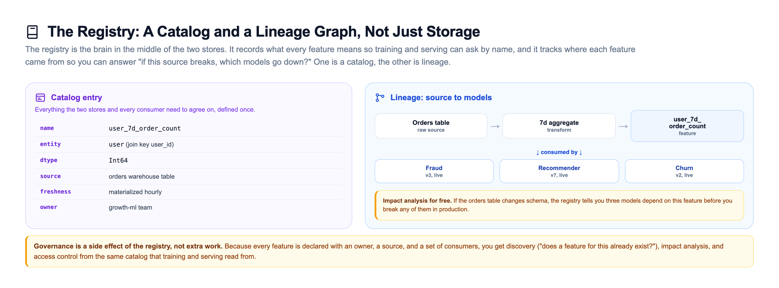
Because every feature is declared with an owner, a source, a type, and a set of consumers, governance stops being separate work and becomes a side effect of the catalog. Discovery falls out of it: before building a new feature, an engineer can search the registry and find that a suitable one already exists. Impact analysis falls out of it: if the upstream orders table changes schema, the registry immediately tells you that three live models depend on a feature derived from it, so you fix them before you break them rather than after. Access control, freshness monitoring, and staleness alerts all hang off the same catalog that training and serving already read from. This is the quiet reason feature stores scale to hundreds of models: the coordination cost of shared features is paid by the registry instead of by people.
Freshness Versus Cost, Feature by Feature
The freshness knob deserves its own look, because setting it wrong is one of the most common and most expensive mistakes teams make with a . The knob is simply how often a feature is materialized into the online store, and it trades staleness against cost along two axes that pull in opposite directions.
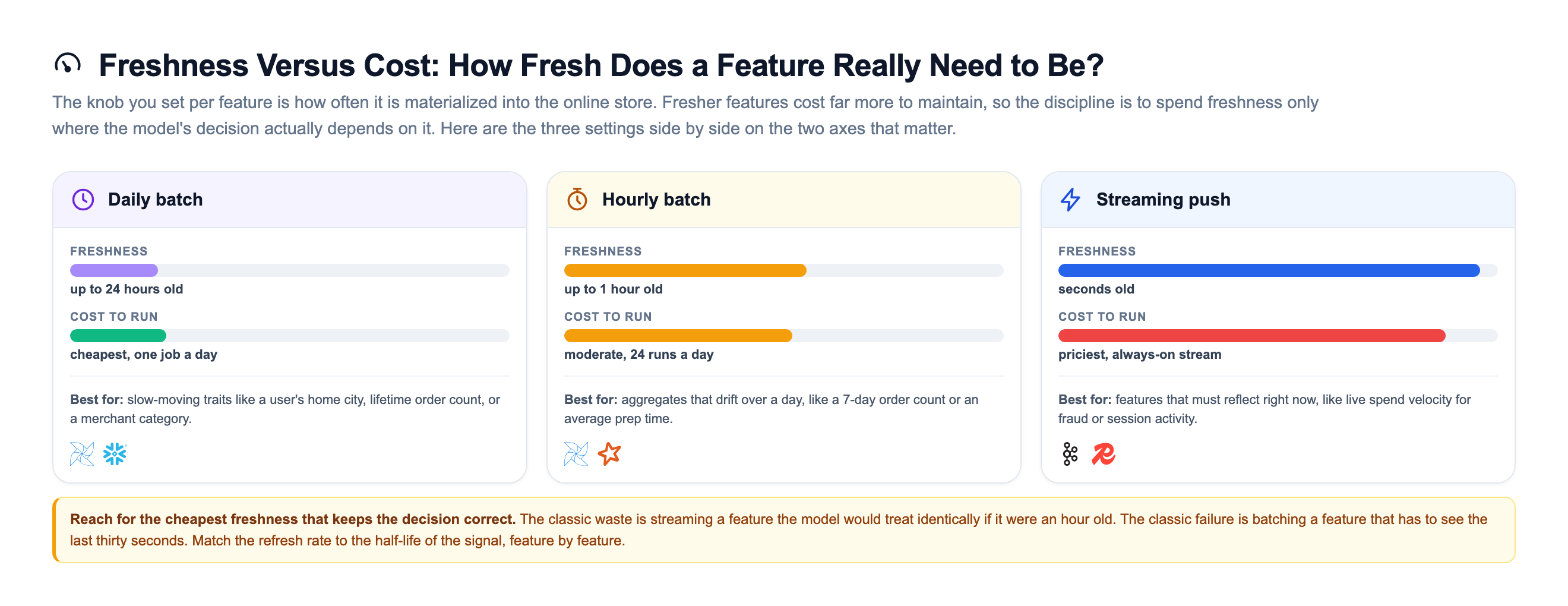
The two failure modes are symmetric. The classic waste is streaming a feature the model would treat identically if it were an hour old, paying for always-on infrastructure to update a number that barely moves. The classic failure is batching a feature that has to see the last thirty seconds, so a fraud model tries to catch an attack that unfolds in ten minutes using features that refresh nightly. Neither is a subtle judgment call once you frame it correctly: match the refresh rate to the half-life of the signal. If the feature's value is meaningfully different an hour from now, it needs streaming. If it is essentially the same tomorrow, batch it and pocket the savings. Doing this per feature, rather than globally, is what keeps a large feature store affordable.
What a Feature Definition Looks Like
Enough theory. Here is a real feature definition in Feast, the reference open-source . The whole point is that this file is the single definition both training and serving obey, so read it as the concrete form of everything above.
First, define the entity, the data source, and the feature view:
# features.py  (the one definition, used by training and serving)
from datetime import timedelta
from feast import Entity, FeatureView, Field, FileSource
from feast.types import Float32, Int64

# The thing features are attached to
driver = Entity(name="driver", join_keys=["driver_id"])

# Where the historical values live (this is the offline store source)
driver_stats_source = FileSource(
    path="s3://feast-demo/driver_stats.parquet",
    timestamp_field="event_timestamp",
)

# The feature definition itself
driver_hourly_stats = FeatureView(
    name="driver_hourly_stats",
    entities=[driver],
    ttl=timedelta(days=7),
    schema=[
        Field(name="conv_rate", dtype=Float32),
        Field(name="avg_daily_trips", dtype=Int64),
    ],
    online=True,          # also serve this from the online store
    source=driver_stats_source,
)
The feature_store.yaml wires up the two stores. Note the offline store and the online store are separate configs, exactly as we drew them:
project: driver_ranking
registry: s3://feast-demo/registry.db
provider: aws
offline_store:
  type: file            # Parquet on S3 for training history
online_store:
  type: redis           # Redis for millisecond serving reads
  connection_string: "redis-prod:6379"
Training builds a dataset with a point-in-time join. You pass in your labeled events, and Feast attaches the correct as-of feature values:
from feast import FeatureStore
store = FeatureStore(repo_path=".")

# labeled_events has columns: driver_id, event_timestamp, label
training_df = store.get_historical_features(
    entity_df=labeled_events,
    features=[
        "driver_hourly_stats:conv_rate",
        "driver_hourly_stats:avg_daily_trips",
    ],
).to_df()   # correct point-in-time features, ready to train on
Serving fetches the latest values by key, in milliseconds, from the online store:
# at request time, inside the serving API
features = store.get_online_features(
    features=[
        "driver_hourly_stats:conv_rate",
        "driver_hourly_stats:avg_daily_trips",
    ],
    entity_rows=[{"driver_id": 1005}],
).to_dict()   # feed straight into model.predict(...)
Same feature names in both calls. Same definition behind both. That is the entire trick, and it is why the skew bug from the first slide is gone. The command, run on a schedule, is what copies the latest values from the Parquet offline store into so has something fresh to read.
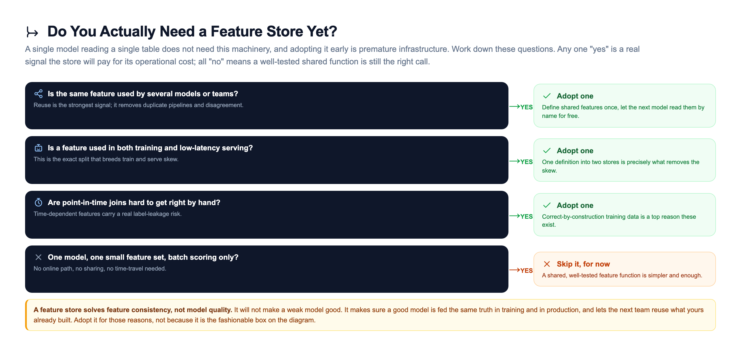
When You Need One, and When You Do Not
A is real infrastructure with real cost. It is not free, and a single model reading a single table does not need one. Adopting it too early is premature infrastructure, so be honest about when it actually pays off. The clearest way to see the tradeoff is to lay the same concerns side by side, handled by ad hoc scripts versus handled by one system.
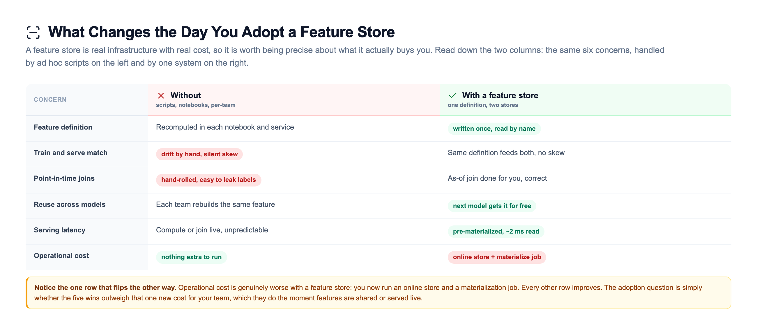
Notice the one row that flips the other way. Operational cost is genuinely worse with a feature store: you now run and pay for an online store like Redis, a materialization job, and the ongoing weight of another system to monitor and keep alive. Every other row improves. So the adoption question reduces to whether the five wins outweigh that one new cost for your situation, and they do the moment features are shared across models or served on a low- path.
The other cost worth naming is latency budget, because it is easy to underappreciate why the online store must be a pre-materialized read rather than a convenient live query.
Freshness is a constant trade-off too: streaming features are fresher but far more expensive to maintain than batch features, as the freshness slide showed. And remember the boundary of what a feature store actually solves. It gives you feature consistency, not model quality. It will not make a bad model good. It makes sure a good model is fed the same truth in training and in production, and that is a different and narrower promise than "better predictions."
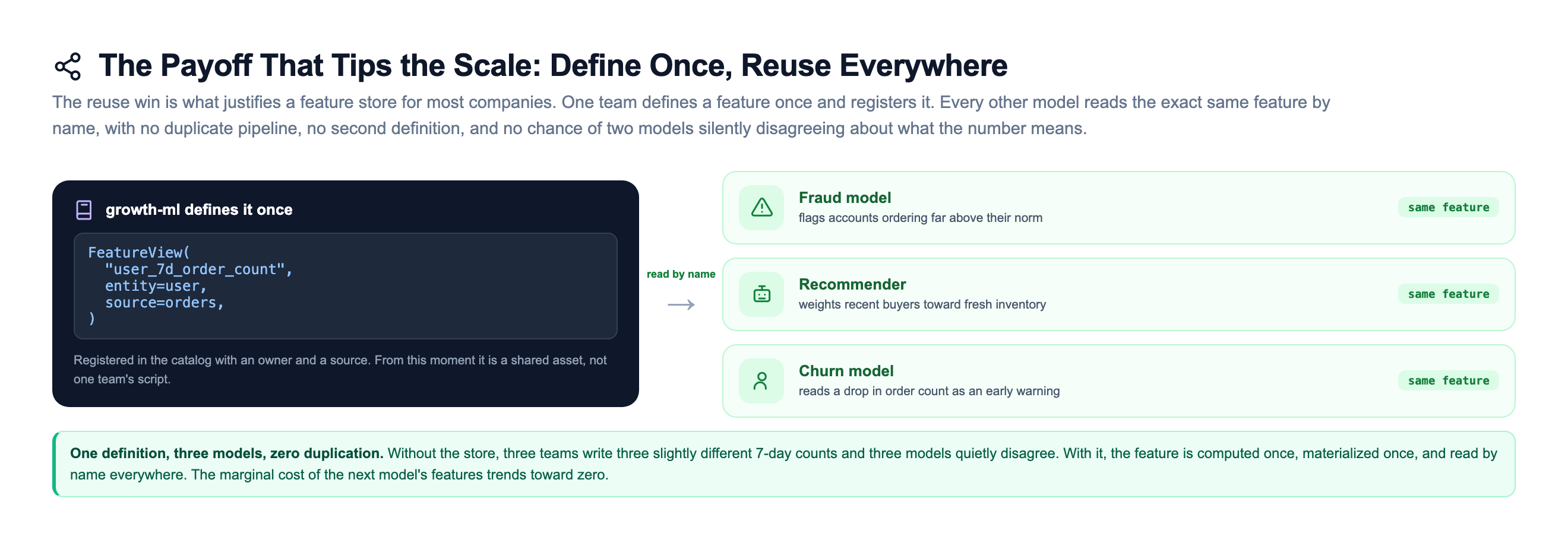
The reuse payoff is usually what tips the scale for a real company, so it is worth seeing on its own.
How the Giants Do It
The whole idea of a was born inside companies feeling this exact pain at scale, and their systems still define the pattern.
Uber built the first widely known one as part of Michelangelo, their internal ML platform. The feature store, called Palette, held thousands of shared features with both an offline half for training and an online half for serving, so hundreds of teams could reuse features instead of each rebuilding them. Michelangelo is the system most people point to as the origin of the pattern, and its offline-plus-online split is exactly the two-store shape from this lesson.
Feast grew out of the same need in the open. It started at Gojek, the Southeast Asian ride-hailing and payments company, together with Google Cloud, and was open-sourced in 2019. It is now the reference open-source feature store, with the offline-store, online-store, registry, and materialization design you saw throughout this lesson. When engineers say "feature store," Feast is usually the concrete thing they picture, and the code on the earlier slide is real Feast.
DoorDash runs a feature store serving billions of predictions per day, with as the online store so their ETA, ranking, and logistics models can read features within a tight request budget. Their scale is a good reminder of why the online path has to be a keyed read: at billions of predictions a day, a two millisecond lookup and a twenty millisecond one are entirely different infrastructure bills. Airbnb built one called Zipline, focused hard on making point-in-time correct training data easy, because label leakage had bitten them enough times to justify a whole system for preventing it.
Different companies, same three lessons. Define features once so training and serving cannot drift. Keep an offline copy for training and an online copy for serving. Join point-in-time so you never leak the future into the past. Get those three right and the skew bug that quietly kills models simply stops happening.
Knowledge Check
Knowledge Check
3 questions - Score 80% to pass
What is train and serve skew?
Why does a feature store keep the same feature in both an offline store and an online store?
What does a point-in-time join prevent when building a training set?