A team wants to specialize a 7 billion parameter open model on their support tickets. The obvious plan is to fine-tune it: keep training the model on their own data until it speaks their domain. So they reach for full fine-tuning, the way you would train any neural network, and update every weight.

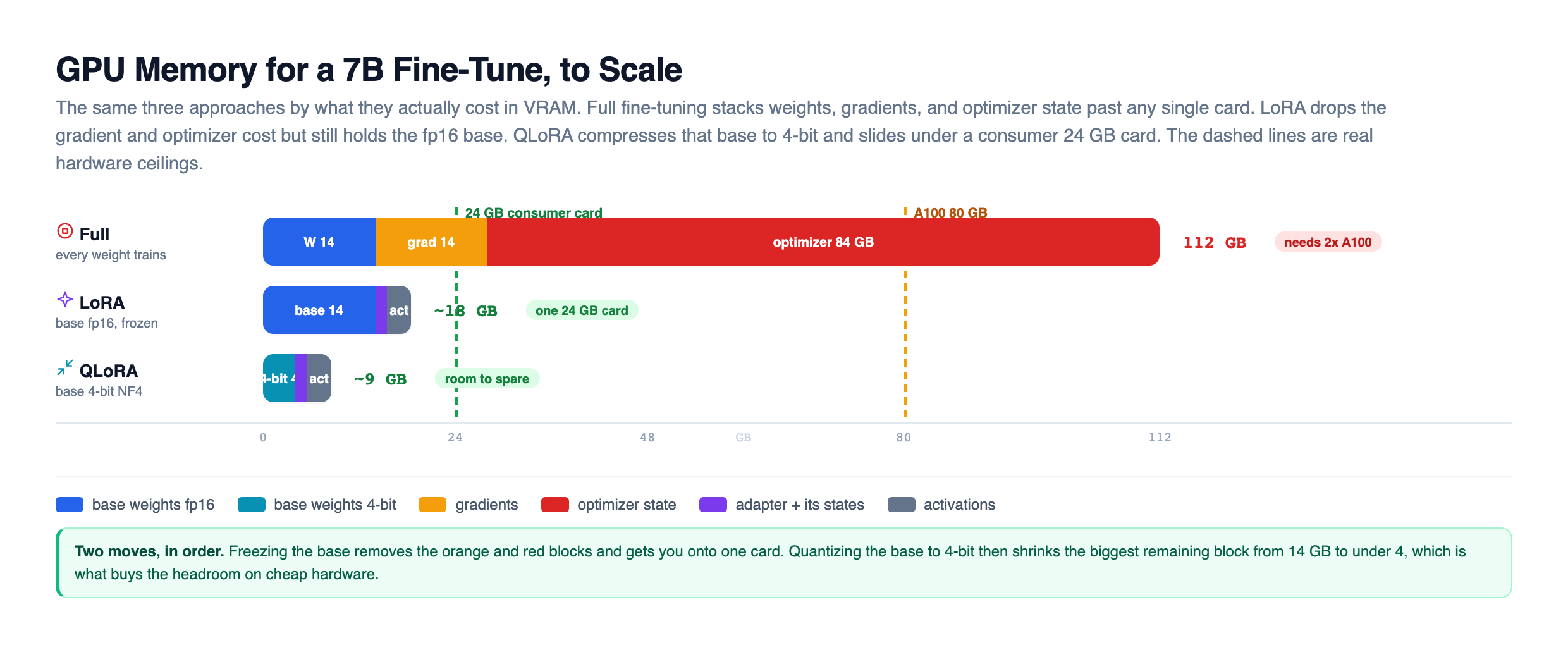
Then they price the hardware, and the number is not what intuition suggests. The weights themselves are the small part of the bill. Holding a 7B model in half precision is about 14 GB. But training with Adam, the standard optimizer, means you also carry a gradient for every weight and three more full-size copies of the model: a first-moment estimate, a second-moment estimate, and a full-precision master copy that mixed-precision training keeps to avoid rounding error accumulating. Those extra copies are held in fp32, which is 4 bytes per number, so each one is roughly 27 GB and the three together come to about 81 GB with the model's exact 6.74 billion weights (6.74 × 4 × 3 is about 80.9). The chart below rounds the model up to a flat 7 billion, which gives 7 × 4 × 3 = 84 GB. Add the fp16 weights and the fp16 gradients and you are already past 100 GB before you count activations, which grow with batch size and sequence length on top.

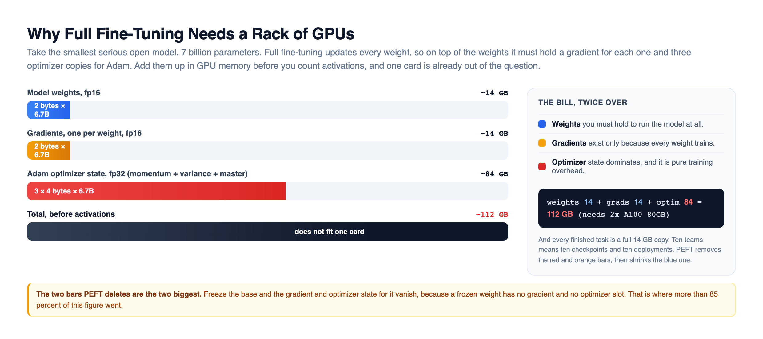
That does not fit on one card. You are renting a multi-GPU box, and the optimizer state you are paying for exists only because every weight is training.

Now the second bill arrives, at deployment. Every fine-tuned model is a full 14 GB copy. The support team wants one model. The sales team wants another. The onboarding team wants a third. Ten teams means ten 14 GB checkpoints, ten deployments, ten copies of nearly the same model sitting in memory and in storage.

Full fine-tuning of a large model is expensive twice over: the training needs a rack of GPUs, and every task produces a full copy of the model.

There is a much cheaper way that gives up almost nothing, and it comes from one sharp observation about what fine-tuning actually changes.

Here is the observation. When you fine-tune a huge pretrained model on a narrow task, you are not rebuilding its knowledge. The base already knows grammar, facts, and reasoning. You are nudging it, applying a small correction so it leans toward your domain. Empirically, that correction turns out to be a low-complexity change, a small adjustment that lives in a tiny subspace even though the model it sits on is enormous.

Parameter-efficient fine-tuning, usually shortened to PEFT, takes that seriously. The recipe is simple to say:

• Freeze the base model. Every one of the 7 billion pretrained weights stays exactly as it is. No gradients, no updates.
• Add a small number of brand-new trainable parameters. These are the only things that learn.
• Train only those. The correction lives entirely in the new parameters.

Because the base is frozen, it carries no gradients and no optimizer state, which is exactly where the optimizer state (about 81 GB, or 84 GB in the chart's rounding) and the 14 GB of gradients went in the last slide. You still hold the base in memory to run it forward, but you stop paying the two costs that dominated the bill. A pleasant side effect comes for free: because the pretrained weights never move, the base cannot forget what it already knew. Full fine-tuning can drift and degrade general capability on data it no longer sees; a frozen base cannot.

The most widely used form of PEFT is called LoRA, short for Low-Rank Adaptation. It is the default across the Hugging Face PEFT library, and it is what most teams mean when they say they fine-tuned an open model. Here is how little actually trains once you switch to it.

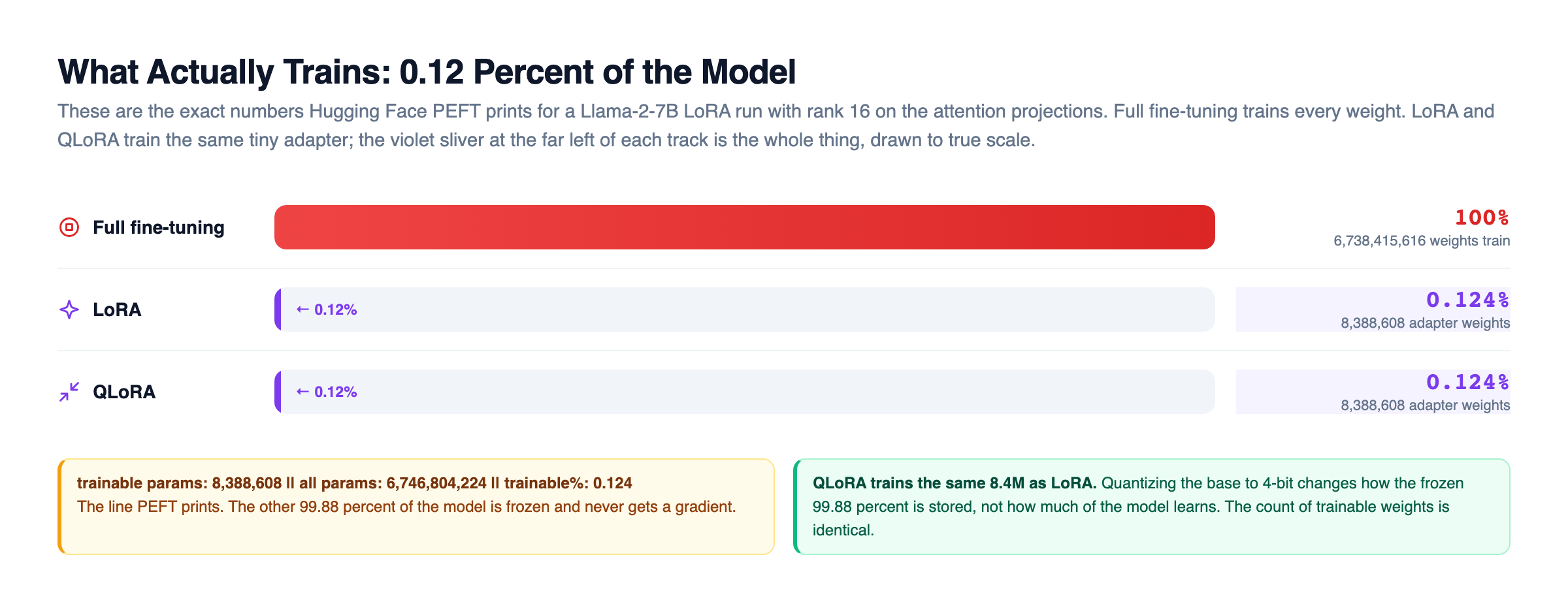
Under one percent of the model learns, and the exact split, 8.4 million trainable against 6.75 billion frozen, is what the library prints when you set this up. Let me show you exactly where those 8.4 million parameters plug in.

A transformer is built from big weight matrices. Inside every attention block there are projection matrices for the query, key, and value. In a 7B model, one of these might be roughly 4096 by 4096, which is about 16.7 million numbers in a single matrix, repeated across dozens of layers. Full fine-tuning would update all of them.

LoRA does not touch those weights. Instead, next to a frozen matrix W, it adds two small matrices:

• A, which projects the input down from the full dimension d to a tiny rank r, say 16.
• B, which projects that rank r representation back up to the full dimension d.

At the forward pass, the input flows through both paths. It goes through the frozen W as normal, and it also goes through A then B. The two outputs are added together. In symbols, the layer computes h = Wx + (alpha / r)(B A x). The frozen path carries the base knowledge. The B A path carries the learned correction.

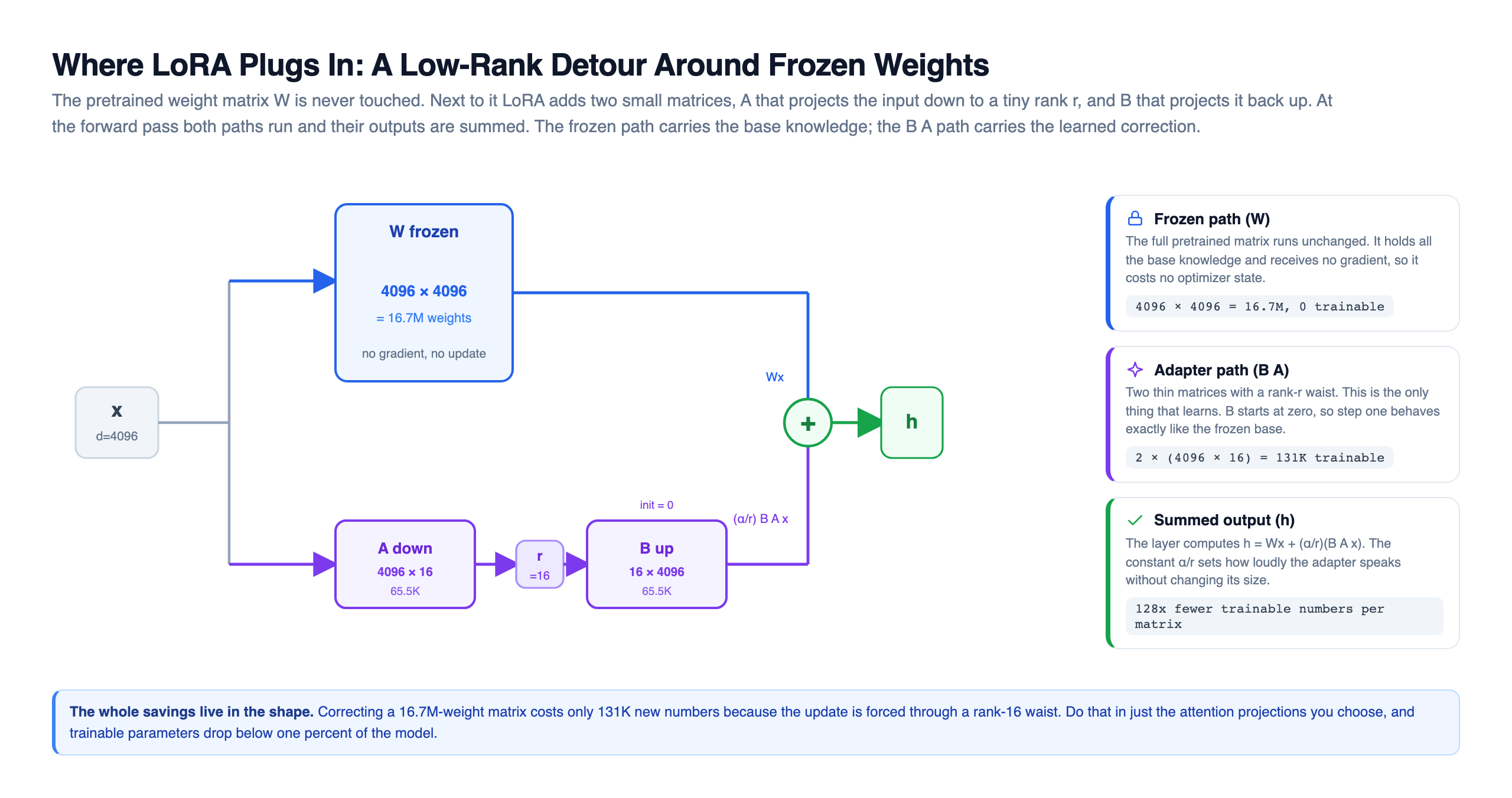
The savings are in the shapes. The frozen matrix W is d x d, so 4096 by 4096 is about 16.7 million numbers. But A maps d down to r, so it is only , and maps r back up to d, so it is only . With r = 16, that is 4096 by 16 twice, about 131 thousand numbers instead of 16.7 million. You are training well under one percent of the size of the matrix you are correcting, and you do that in only the layers you choose, usually just the attention projections.

LoRA already cut the gradient and optimizer costs to almost nothing. But one big number was left standing: you still hold the frozen base in memory. At 14 GB for a 7B model in fp16, that base is now the thing keeping you off a single small GPU.

QLoRA attacks exactly that. The insight is that the base is frozen, so it never gets updated, so it does not need to be stored in high precision. You can compress it hard and only unpack it when you need to run a layer.

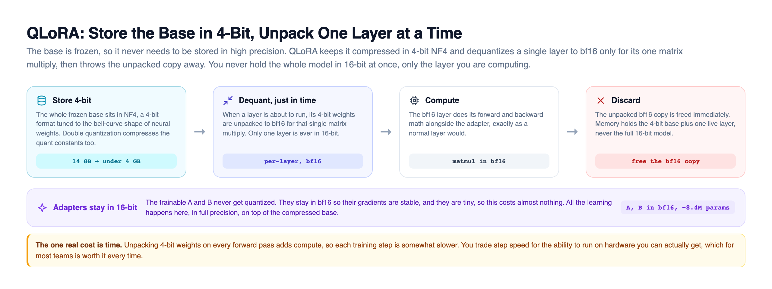
QLoRA does three things. It quantizes the frozen base to 4-bit using a format called NF4, short for NormalFloat 4-bit, whose 16 levels are placed to match the bell-curve shape that neural network weights actually follow, so it loses less information than a naive 4-bit rounding. It keeps the trainable A and B in bf16, so their gradients stay stable, and since they are tiny this costs almost nothing. And it dequantizes just in time: when a layer runs, its 4-bit weights are unpacked to bf16 for that one matrix multiply, used, and thrown away, so you never hold the whole model in 16-bit at once, only one layer at a time. QLoRA adds one more trick called double quantization, which quantizes the quantization constants themselves to shave off a further fraction of a gigabyte.

The result is dramatic. The QLoRA paper showed you could fine-tune a 65B model on a single 48 GB GPU, and a 7B fine-tune drops onto a consumer 24 GB card. There is a real cost: dequantizing 4-bit weights on every forward pass adds compute, so each training step is somewhat slower, and the effect is larger for compute-bound layers. You are trading time for the ability to run on hardware you can actually get. For most teams that is a trade worth making every time, and it is often paired with gradient checkpointing to trade a little more compute for even lower activation memory.

Here is a QLoRA setup with the Hugging Face stack: transformers loads the base quantized to 4-bit, and peft wraps the attention projections with LoRA adapters. This is close to what most teams actually run in PyTorch.

from peft import LoraConfig, get_peft_model, prepare_model_for_kbit_training
from transformers import AutoModelForCausalLM, BitsAndBytesConfig
import torch

# 1. Load the 7B base, quantized to 4-bit NF4 (this is the QLoRA part)
bnb_config = BitsAndBytesConfig(
    load_in_4bit=True,
    bnb_4bit_quant_type="nf4",            # NormalFloat, tuned for weight shape
    bnb_4bit_compute_dtype=torch.bfloat16, # dequantize to bf16 per layer
    bnb_4bit_use_double_quant=True,        # quantize the quant constants too
)
base = AutoModelForCausalLM.from_pretrained(
    "meta-llama/Llama-2-7b-hf",
    quantization_config=bnb_config,
    device_map="auto",
)
base = prepare_model_for_kbit_training(base)

# 2. Describe the LoRA adapters: the ONLY weights that will train
lora_config = LoraConfig(
    r=16,                 # rank of the adapter matrices
    lora_alpha=32,        # scaling; effective strength = alpha / r = 2.0
    target_modules=["q_proj", "v_proj"],  # inject into attention projections
    lora_dropout=0.05,
    bias="none",
    task_type="CAUSAL_LM",
)

model = get_peft_model(base, lora_config)
model.print_trainable_parameters()
# trainable params: 8,388,608 || all params: 6,746,804,224 || trainable%: 0.124

Read that last line. Out of about 6.75 billion parameters, only 8.4 million train. That is 0.124 percent. The other 99.88 percent are frozen. Those five lines of LoraConfig are the whole training pipeline in miniature, and the flow behind them is worth seeing laid out.

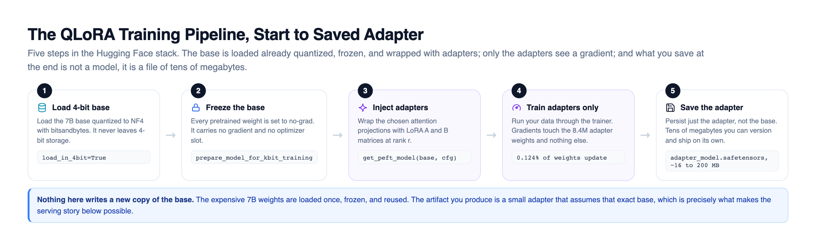
When training finishes, you save just the adapter, a file of tens of megabytes, not a 14 GB model. The r, , and fields are the knobs you will spend the most time on. Rank in particular has a shape worth internalizing before you go turning it up.

The playground did the counting for you. Here is the same counting with a pencil, so that you can check any LoRA setup yourself, without trusting a library printout. I use the numbers from the config above: hidden size 4096, 32 layers, rank 16, and two target matrices per layer, q_proj and v_proj.

Step 1: one adapter. Matrix A has shape 16 by 4096, which is 16 × 4096 = 65,536 numbers. Matrix B has shape 4096 by 16, also 65,536 numbers. Together that is 2 × 65,536 = 131,072 numbers. The frozen matrix beside it is 4096 × 4096 = 16,777,216 numbers. So the adapter is 16,777,216 ÷ 131,072 = 128 times smaller than the matrix it corrects.

Step 2: the whole model. There are 2 adapters in each layer and 32 layers, so 131,072 × 2 × 32 = 8,388,608 trainable numbers. That is exactly the "trainable params" line the PEFT library printed. The "all params" line is the base plus the adapters: 6,738,415,616 + 8,388,608 = 6,746,804,224. And 8,388,608 ÷ 6,746,804,224 is about 0.00124, which is the 0.124 percent.

Step 3: memory for full fine-tuning. Count bytes for each weight. fp16 weights take 2 bytes. fp16 gradients take 2 bytes. The three fp32 Adam copies take 4 bytes each, so 12 bytes. That is 2 + 2 + 12 = 16 bytes for every weight. Multiply by 6.74 billion weights and you get about 108 GB, before activations. The chart's 112 GB is the same sum with the model rounded to 7 billion: 7 × 16 = 112.

Step 4: memory for QLoRA. The base is stored in 4 bits, which is half a byte, so 6.74 billion × 0.5 is about 3.4 GB. The adapter trains in the normal way, so it carries its own weights, gradients and optimizer copies, the same 16 bytes each: 8,388,608 × 16 is about 0.13 GB. The total is about 3.5 GB before activations. From about 108 GB to about 3.5 GB is roughly 30 times less memory (108 ÷ 3.5 is about 31), and every step of that came from two choices: freeze the base, then store it small.

One thing this count leaves out, on purpose, is activations. These are the values each layer computes during the forward pass and keeps for the backward pass. They grow with batch size and sequence length, not with rank, which is why the memory chart adds a few GB on top of these sums.

The memory savings during training are only half the story. The other half changes how you deploy.

Because every fine-tuned task is now a tiny adapter instead of a full model, you can keep one copy of the expensive base in GPU memory and swap small adapters on top of it per request. The support-team adapter, the sales adapter, the onboarding adapter: they all share the same 7B base weights that are already loaded.

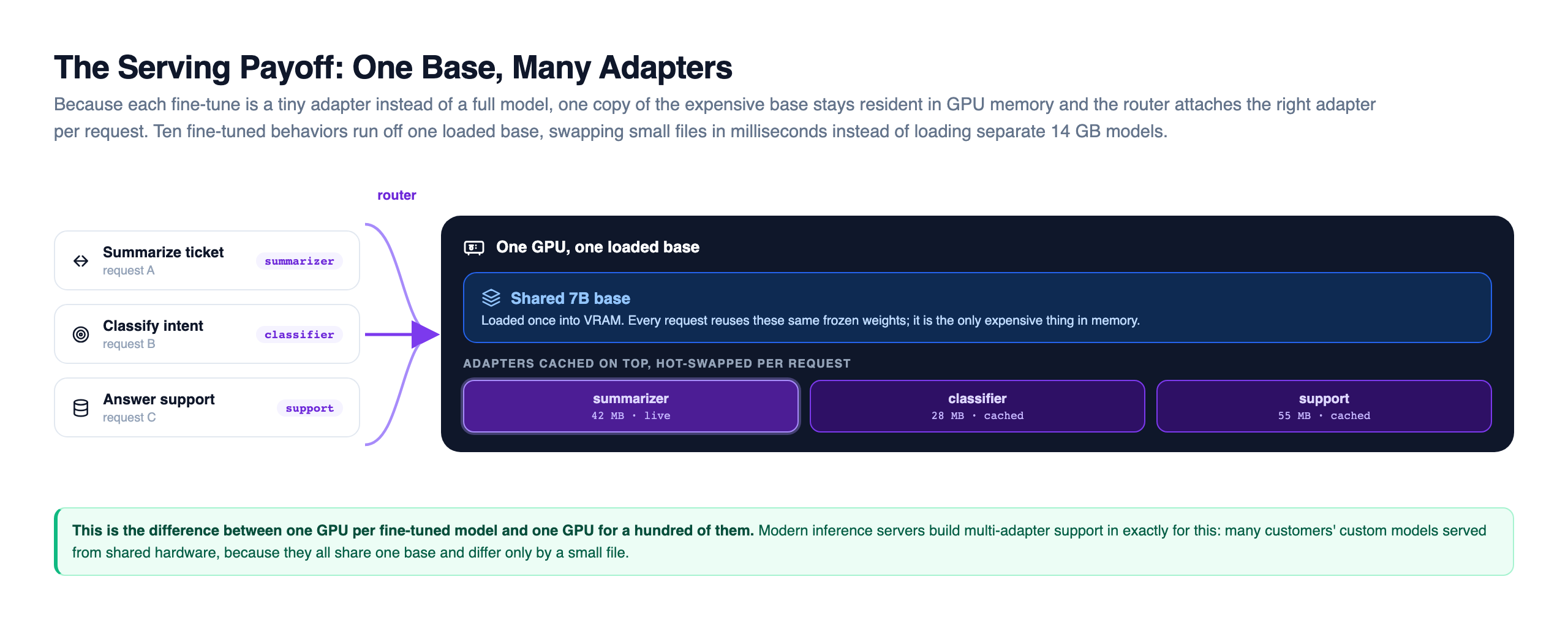
Follow the flow. A summarization request comes in, the router attaches the summarizer adapter, and the base plus that adapter answers. A classification request from the same server swaps to the classifier adapter, which is already cached, in milliseconds. Ten fine-tuned behaviors run off one loaded base model.

Compare that to full fine-tuning, where each task is a separate 14 GB model that needs its own memory and its own deployment. With adapters, ten tasks might cost you the base plus ten small files. Serving systems built for this, like the multi-adapter support in modern inference servers such as vLLM and dedicated runtimes like S-LoRA, lean on exactly this property. They batch requests that use different adapters against the same base weights, applying each adapter only to its own rows, so a single deployment serves many customers' custom models from shared GPU memory. This is the difference between one GPU per fine-tuned model and one GPU for a hundred of them.

Here are the three approaches lined up side by side, so the choice has a shape before we walk it.

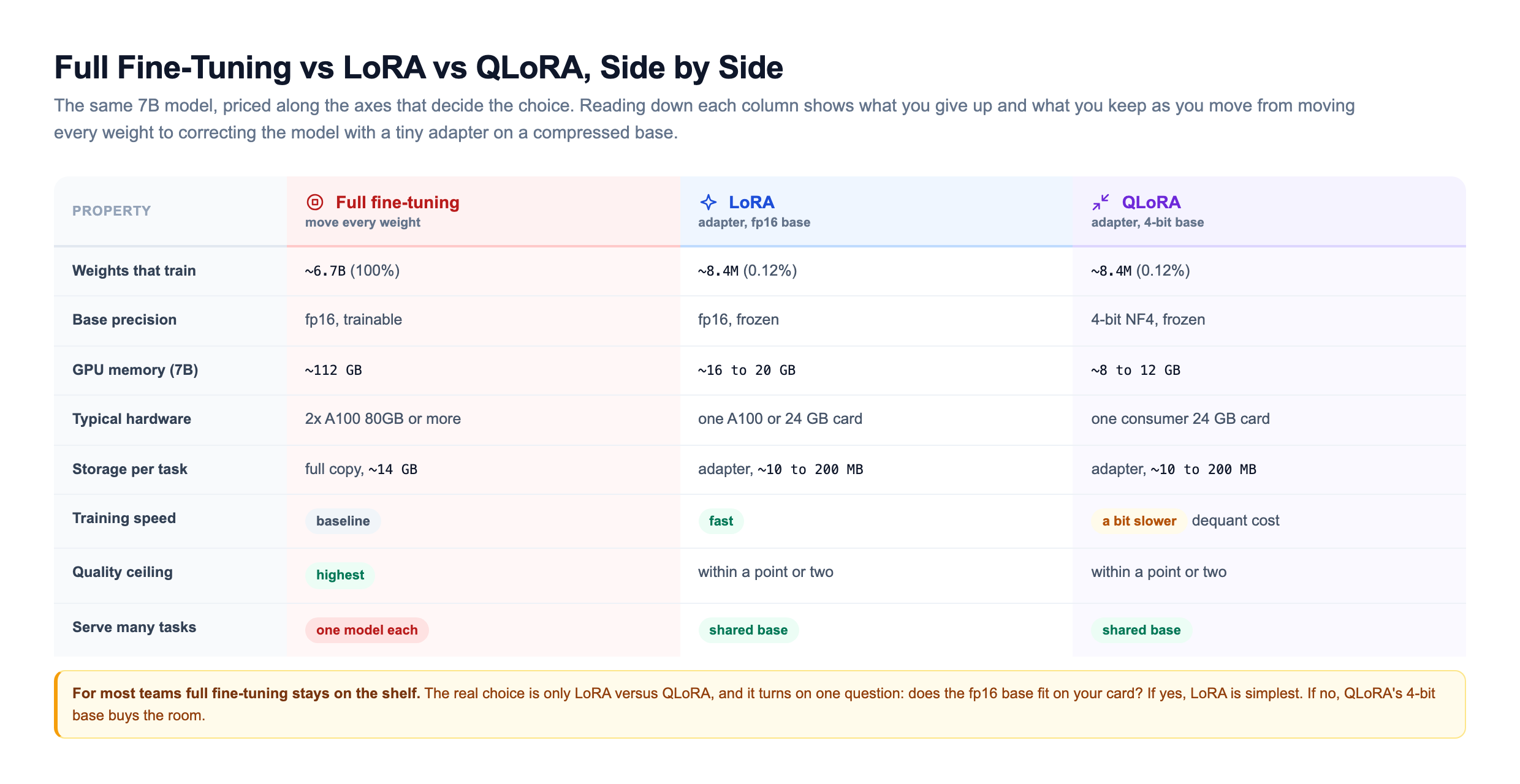
The single row that decides most real projects is GPU memory, so it is worth seeing to scale. Freezing the base removes the gradient and optimizer blocks that dominated full fine-tuning; quantizing the base then shrinks the largest remaining block.

The picture makes the honest recommendation obvious, and it follows straight from where each bar lands against the hardware you can buy.

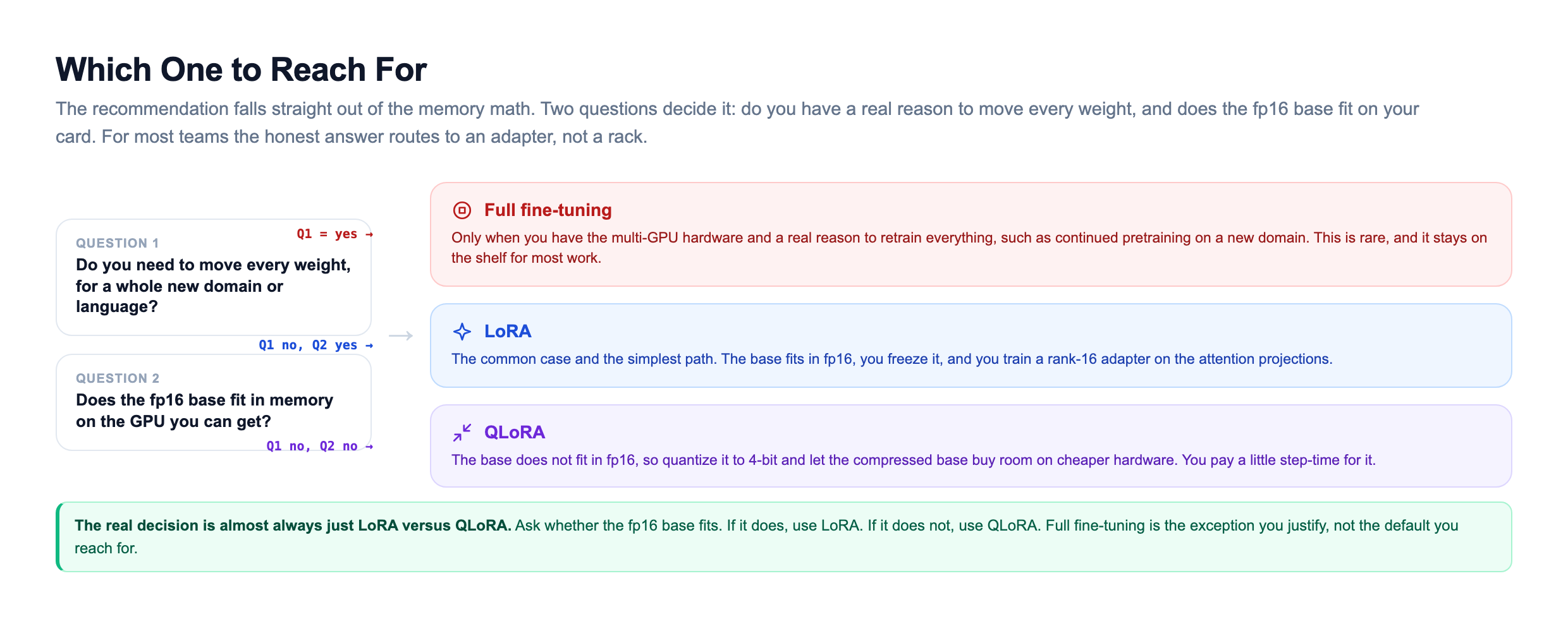
Use full fine-tuning only when you have the multi-GPU hardware and a real reason to move every weight, such as continued pretraining on a whole new domain or language where the model genuinely has to absorb new knowledge rather than adjust behavior. That is rare. Reach for when the base fits in fp16 on your card, which is the common case and the simplest path. Reach for when it does not fit, and let the 4-bit base buy you room on cheaper hardware. For most teams, full fine-tuning stays on the shelf and the real choice is only LoRA versus QLoRA.

These are general pitfalls that follow from the basic mechanics in this lesson. I keep to those basics here; the details of any one library change from version to version, so check its documentation before you rely on a setting.

Using an adapter on a different base. An adapter is a correction to one exact set of frozen weights. The numbers in A and B only make sense added to the W they were trained beside. Load the same adapter on a different base model, even one with the same shape, and the correction no longer fits. Always record which base an adapter was trained on, and ship that name with the file.

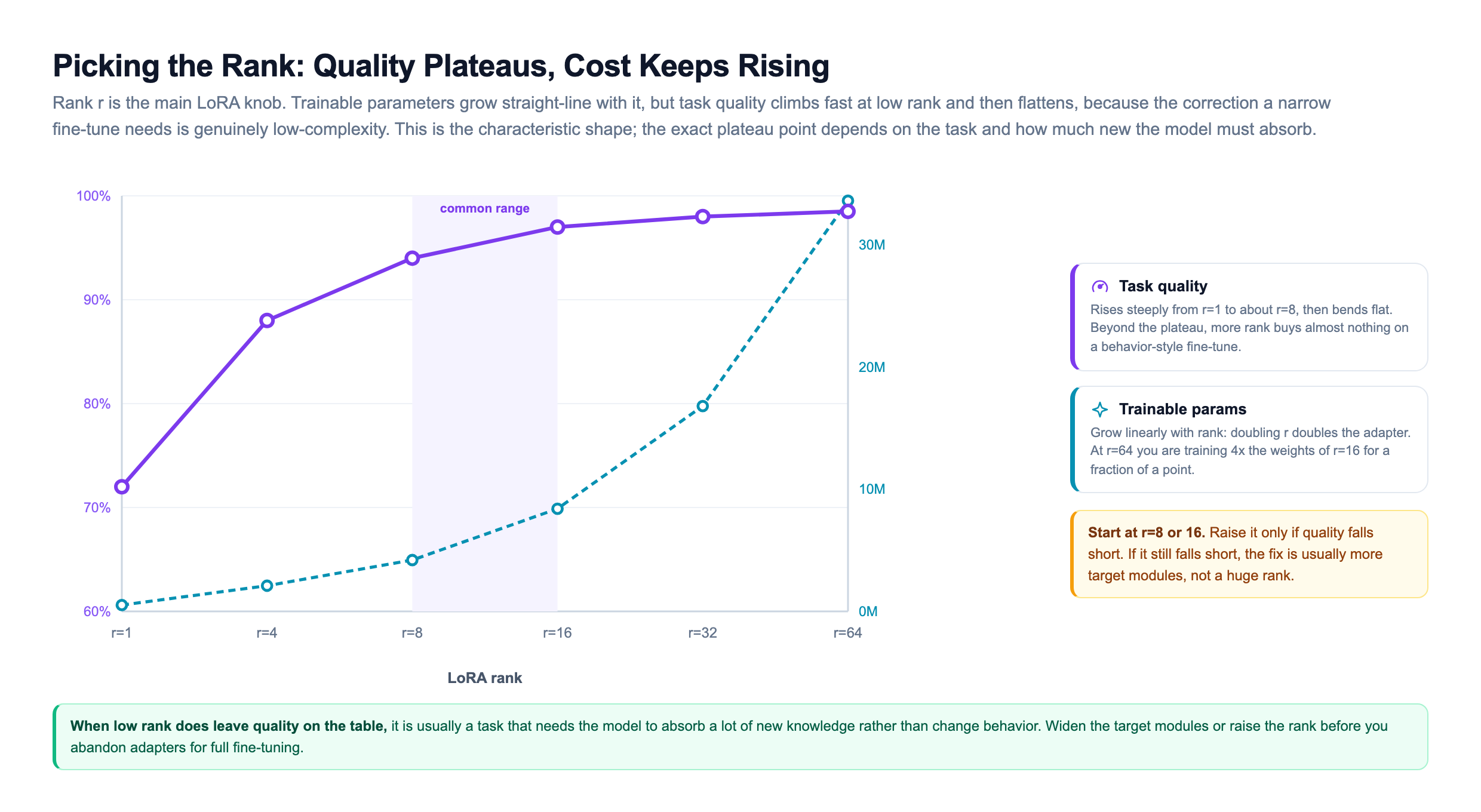
Raising the rank before looking at the data. When quality falls short, the reflex is to turn r up. The rank chart showed that quality flattens early, so a bigger rank often buys very little. Check the training examples first. Wrong or inconsistent examples teach the wrong behavior at any rank.

Using LoRA to add facts. The last lesson made this point for fine-tuning in general, and it holds for LoRA too. A low-rank correction is good at shaping behavior, like a format or a tone. Facts that change belong in retrieval.

Reading the memory sums as the whole bill. The by-hand sums leave out activations, and so does the playground. A setup that fits on paper can still run out of memory with long sequences or a large batch. Test with your real sequence length before you book the hardware.

You do not have to take the theory on faith. Adapters are how the open-model world actually ships fine-tunes.

Hugging Face made LoRA the default through its PEFT library, and the Hub now hosts an enormous number of small adapter files, each one a fine-tune of a shared base like Llama or Mistral. Downloading a specialization is often a few tens of megabytes, not tens of gigabytes, precisely because the base is shared. LoRA is also only one branch of a wider family, and it helps to know the neighbors when a task pushes on a constraint LoRA does not address.

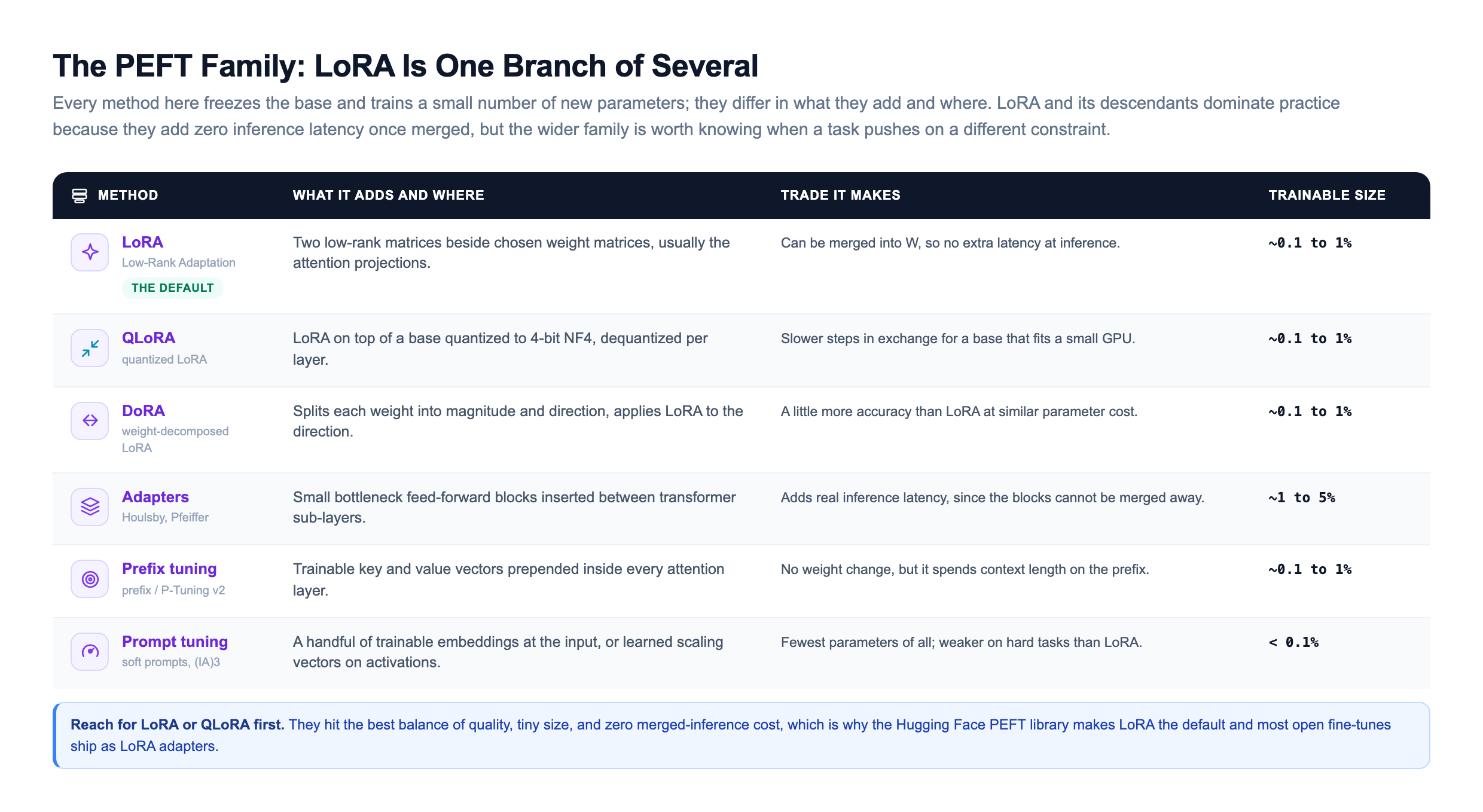
The QLoRA result from 2023 is the reason a huge wave of open fine-tunes exists at all. By proving you could fine-tune a 65B model on a single 48 GB GPU, it put serious fine-tuning within reach of individual researchers and small teams instead of only large labs with GPU clusters. A great deal of the community fine-tuning that followed ran on QLoRA on one card.

Modern inference servers built the multi-adapter idea into serving. Instead of loading a separate copy of the model per fine-tune, they load one base and hot-swap LoRA adapters per request, so a single deployment can serve many customers' custom models from shared GPU memory. That is the adapter-swapping picture from earlier, running in production.

The through-line is the same one you started with. The expensive thing is the base model. PEFT lets everyone share it, correct it cheaply with tiny adapters, and serve dozens of specializations off one loaded copy. That is why parameter-efficient fine-tuning went from a clever trick to the default way large models get adapted.