The Search Box That Understands Meaning
A support team at a SaaS company has 40,000 help articles. A customer types "I was charged twice this month." There is no article with that exact phrase. The article that answers it is titled "Understanding duplicate transactions and refunds." A keyword search finds nothing useful, because the customer and the writer used completely different words for the same idea.
This is the problem every system, every semantic search box, and every recommendation feed runs into. You do not want to match words. You want to match meaning. And meaning does not live in the letters, so a normal database index, which is brilliant at finding an exact string or a number range, is useless here.
The fix is to turn every article and every query into an , a list of numbers that captures meaning, and then find the articles whose numbers are closest to the query's numbers. Do that and "charged twice" lands right next to "duplicate transactions" even though they share no words.
That single move, from matching text to finding nearest points in space, is what a exists to do, and it is the retrieval backbone under almost every LLM feature shipping today. This lesson walks the whole layer from the ground up: how text becomes a point, why the obvious exact search collapses at scale, the three index families that rescue it, and the operational details, filtering, sharding, and choosing a store, that decide whether it works in production or falls over on the first real query.
Embeddings Are Points, Similarity Is Distance
An model takes a chunk of text and returns a fixed-length list of numbers, called a vector. OpenAI's text-embedding-3-small returns 1536 numbers. A sentence-transformers model might return 384 or 768. That count is the number of dimensions, and it is fixed for a given model: every string you embed, one word or one page, comes back as the same size vector.
Here is the mental model that makes everything else click. Think of a 2D scatter plot, where every point has an x and a y. Now imagine that same plot with 1536 axes instead of 2. Each embedding is one point in that 1536-dimensional space. The model is trained so that texts with similar meaning end up as points close together, and unrelated texts end up far apart. "Refund" and "money back" sit near each other. "Refund" and "photosynthesis" sit at opposite ends.
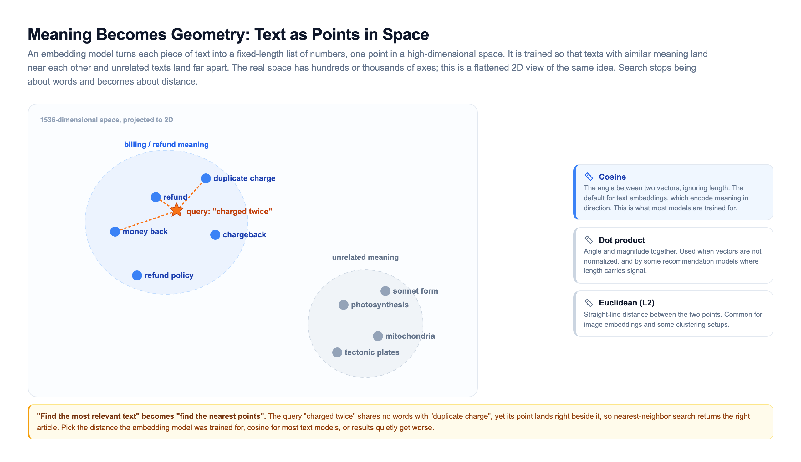
So "find the most relevant articles" becomes a geometry question: find the points nearest to the query point. That is nearest-neighbor search, and it is the whole job.
"Nearest" needs a definition of distance. Three are common, and they are not interchangeable:
| Distance | What it measures | When it is used |
|---|---|---|
| Cosine | The angle between two vectors, ignoring length | The default for text embeddings, which care about direction not magnitude |
| Dot product | Angle and length together | When vectors are not normalized, or for some recommendation models |
| Euclidean (L2) | Straight-line distance between the points | Image embeddings and some clustering setups |
Pick the distance the embedding model was trained for. For most text models that is cosine. Use the wrong one and your results do not error out, they quietly get worse, which is the most expensive kind of bug because nobody notices it in a demo. If you normalize your vectors to unit length, cosine and dot product rank results identically, which is why many production setups normalize once at ingest and then use the cheaper dot product at query time.
Why You Cannot Just Compare Every Vector
The obvious way to find the nearest neighbors is to compare the query against every stored vector, keep a running list of the closest, and return the top few. This is called brute-force or flat search, and it has one great property: it is exact. It always returns the true nearest neighbors, every time.
It also does not scale. Comparing against every vector is O(n): double the number of vectors and you double the work. Worse, each comparison is a math operation across every dimension. One over a 1536-dimensional vector is about 1536 multiply-add operations, so the cost is really O(n times d), and both factors grow as your product does.
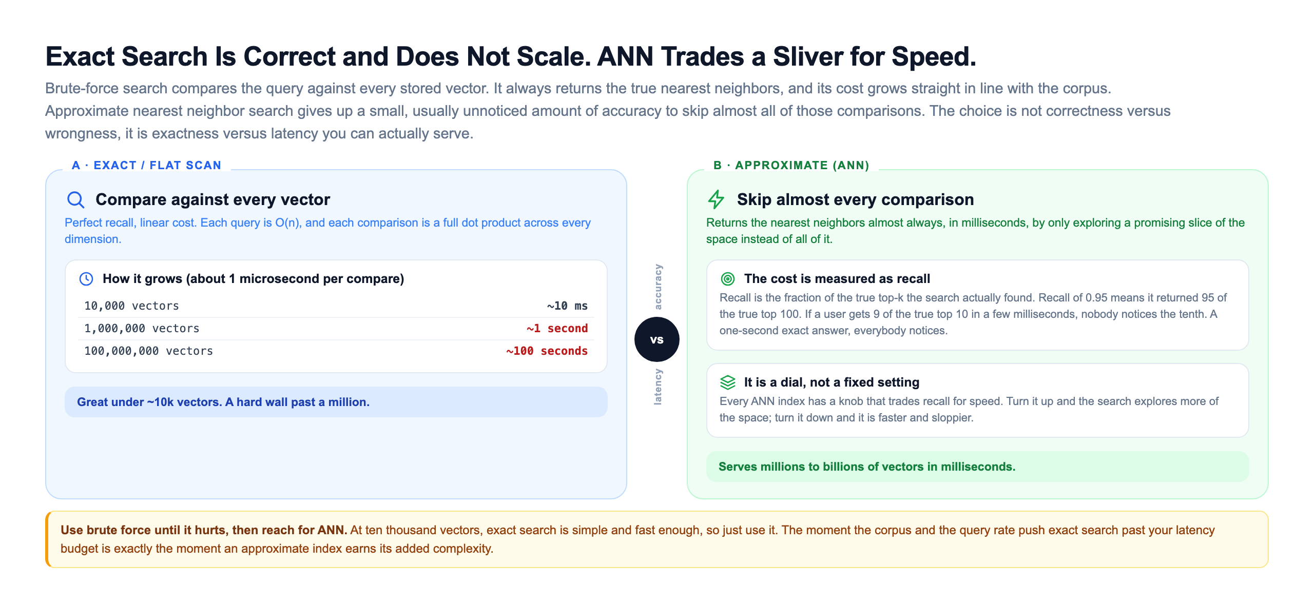
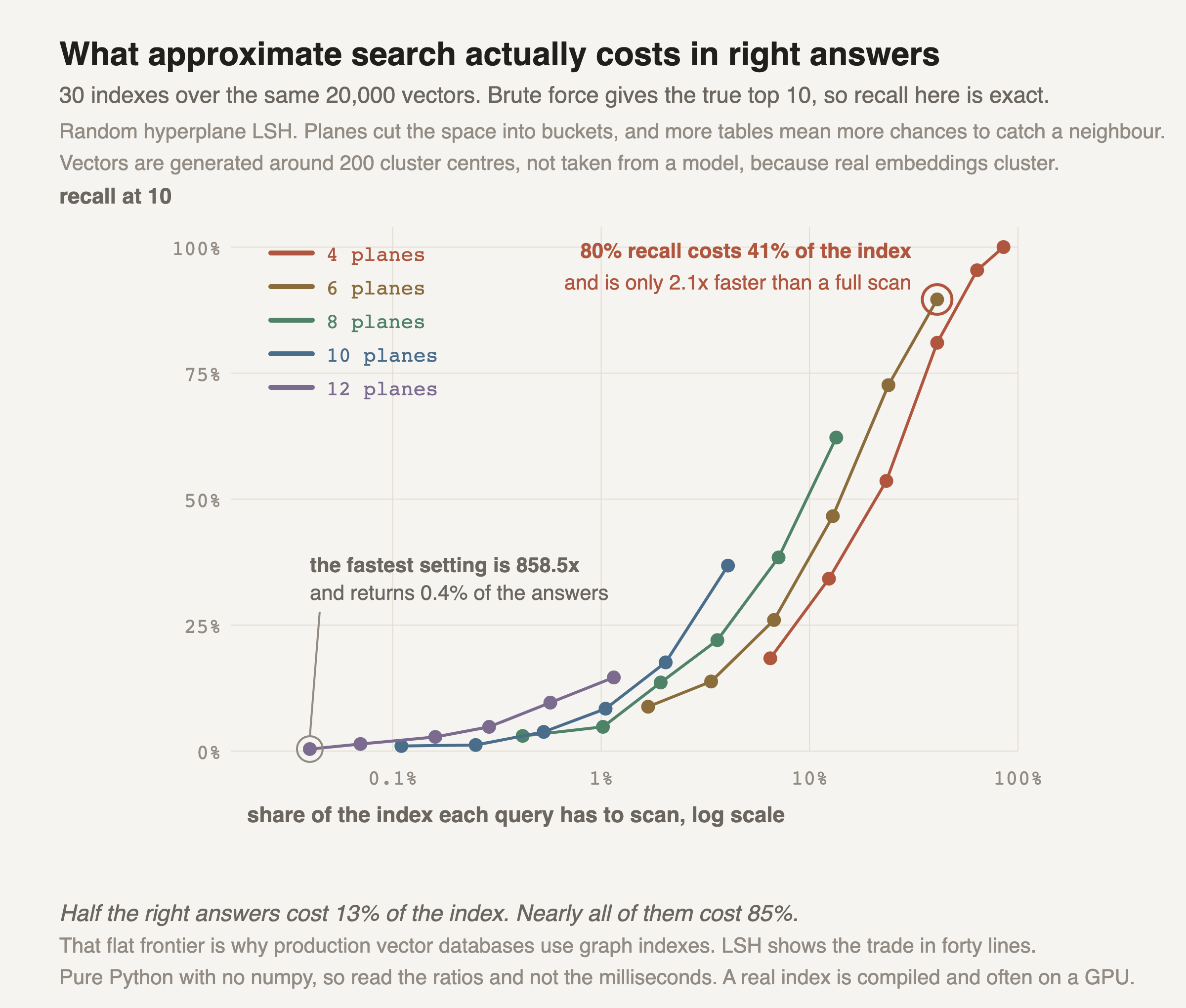
At ten thousand vectors, brute force is fine, and honestly you should just use it. Standing up an approximate index at that size adds complexity you do not need and can even be slower once you count the index overhead. At a million vectors it is already too slow for a live request, and at a hundred million it is hopeless, now multiply by thousands of queries per second arriving at once. Exact search hits a wall, and the shape of that wall, a straight line that only climbs with corpus size, is why the entire field of exists.
The trap to avoid is treating this as a premature-optimization question. It is a step function, not a gradient. Under ten thousand vectors, use the simplest thing. The moment your corpus and query rate push exact search past your budget, that is precisely the moment an approximate index stops being over-engineering and becomes the only thing that works.
The Trade: A Little Accuracy for a Lot of Speed
The insight behind (ANN) search is simple and a little uncomfortable: you do not actually need the exact nearest neighbors. You need the nearest neighbors almost always, and you need them fast.
If a search returns 9 of the true top 10 and one slightly-less-relevant article in the tenth slot, no user notices. But if it takes a full second, every user notices. So ANN indexes give up a sliver of accuracy to skip almost all of the comparisons, and the sliver is usually invisible while the speedup is not.
We measure that sliver with recall: of the true top-k nearest neighbors, what fraction did the search actually find? Recall of 0.95 means it found 95 of the true top 100. The whole game of ANN is buying high recall at low , and it is a dial you set, not a property you accept. Every ANN index has a knob that trades recall for speed. Turn it up and the search explores more of the space, so recall climbs but latency grows. Turn it down and it is faster but sloppier.
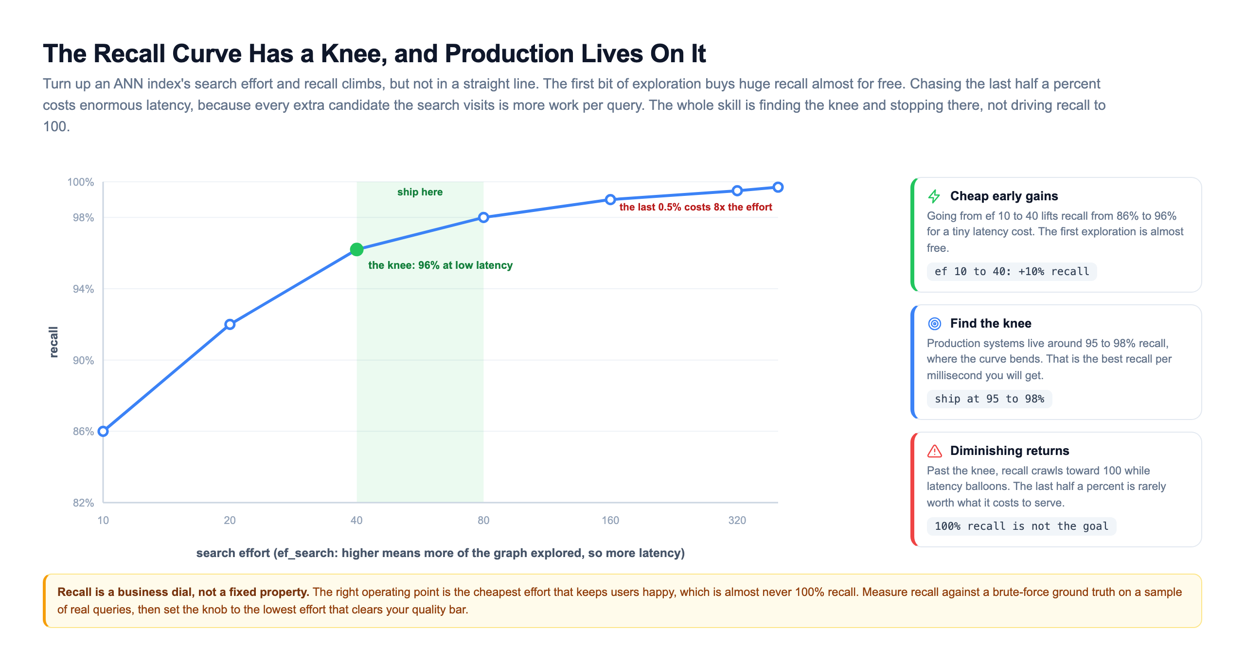
The curve is not linear, and understanding its shape is most of the job. The first bit of exploration buys huge recall almost for free: going from a tiny search width to a modest one can lift recall ten points for a barely measurable latency cost. Chasing the last half a percent, by contrast, costs enormous latency, because past the knee every extra candidate the search visits is more work per query for almost no gain.
The key skill is finding the knee of that curve and stopping there. Production systems live near the knee, usually around 95 to 98 percent recall, not at 100. And recall is not something you eyeball, it is something you measure: run a sample of real queries through both brute force and your index, compare the result sets, and compute the fraction that match. That number is your recall, and you tune the knob to the cheapest setting that clears your quality bar.
The Three Ways to Build an ANN Index
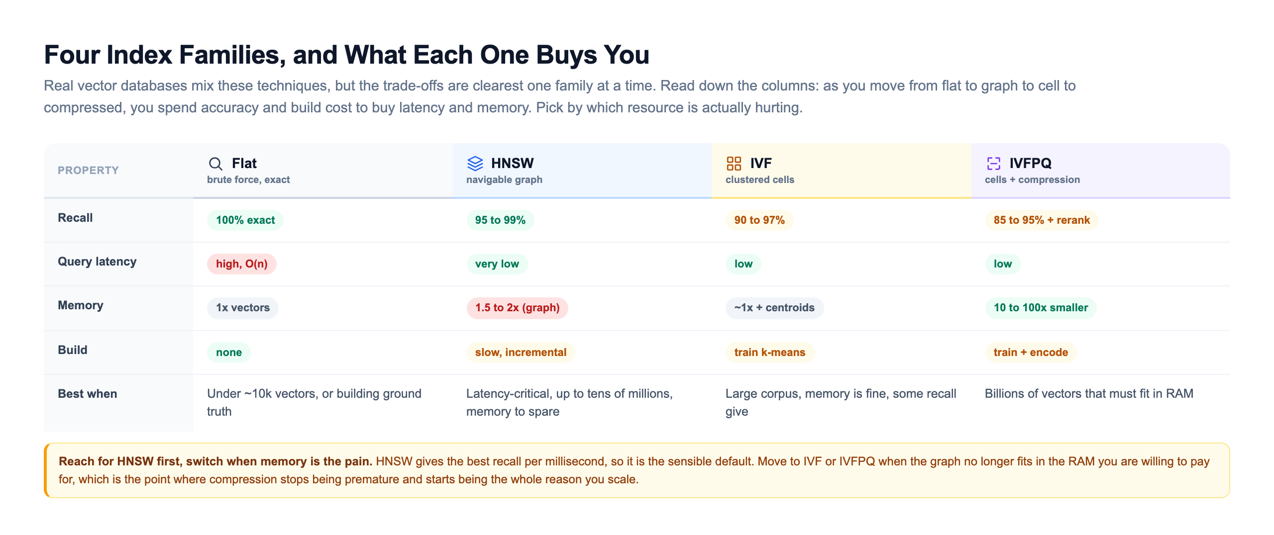
There are three core techniques, and real vector databases mix them. You should know what each one does, because the right choice depends on which resource, or memory, is actually hurting.
(Hierarchical Navigable Small World) builds a layered graph. Every vector is a node connected to its nearest neighbors. There is a stack of layers: the top layer is sparse with long-range links, and each layer down is denser with shorter links. A search starts at the top, takes big greedy hops toward the query to get into the right region fast, then drops down a layer and refines. Highway, to arterial road, to side street.
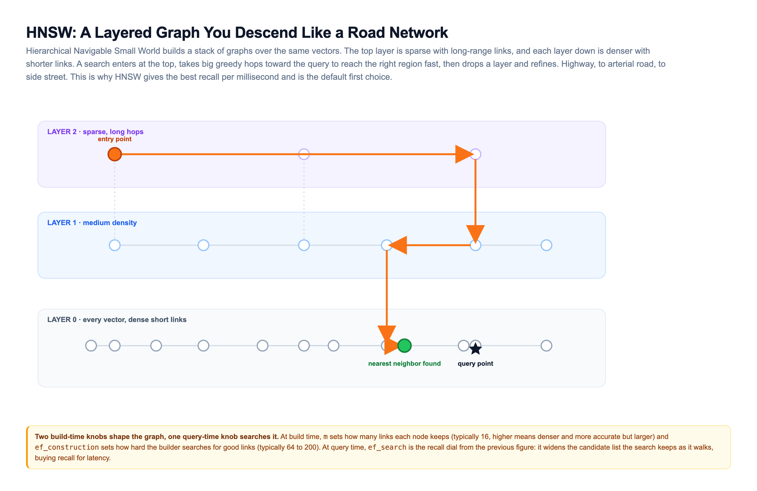
HNSW has three knobs worth knowing. At build time, m sets how many links each node keeps (16 is a common default; higher makes the graph denser, more accurate, and larger in memory), and ef_construction sets how hard the builder searches for good links (64 to 200 is typical; higher builds a better graph but takes longer). At query time, ef_search is the recall dial from the previous slide: it controls how wide a candidate list the search keeps as it walks, so raising it buys recall at the cost of latency.
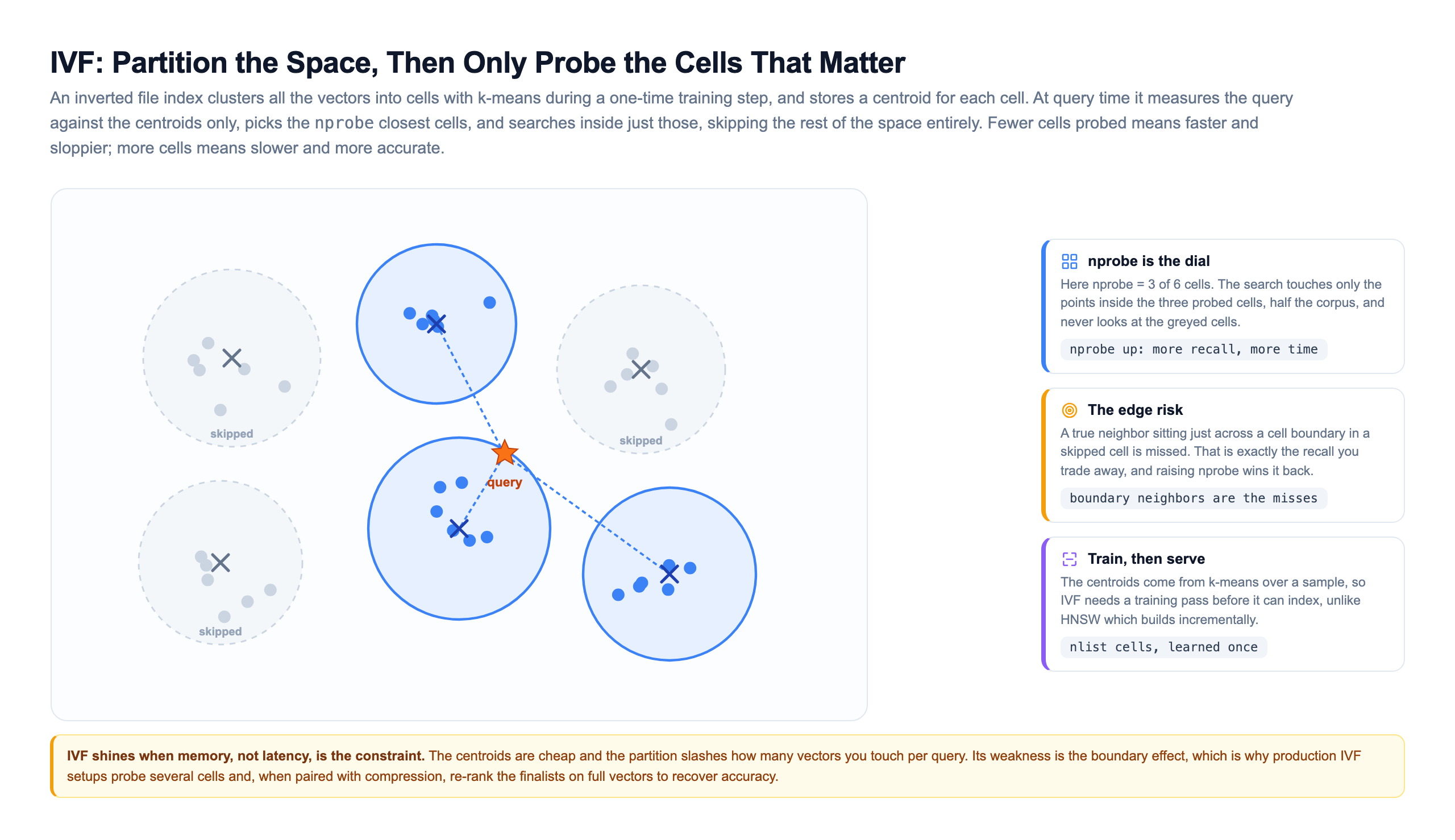
IVF (Inverted File) clusters all the vectors into cells using k-means during a training step. Each cell has a centroid. At query time you only search the nprobe cells whose centroids are closest to the query, and skip the rest of the space entirely. Fewer cells searched means faster and sloppier; more cells means slower and more accurate.
The Write Path: Turning a Corpus Into an Index
Everything so far is about answering a query. But before a single query runs, the corpus has to be turned into vectors and built into an index, and the decisions you make on this write path shape retrieval quality more than any query-time tuning ever will.
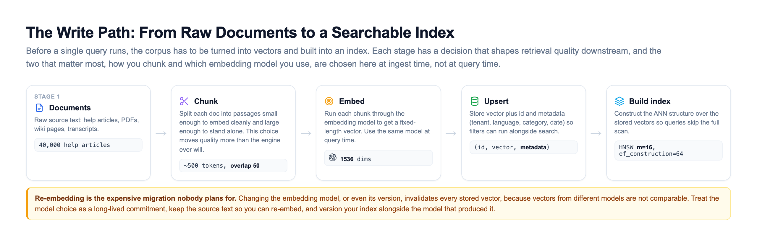
Two of these stages carry almost all the weight. Chunking decides what a single searchable unit is. Too large and a chunk covers several topics, so its single vector is a blurry average that matches nothing well. Too small and it loses the surrounding context that made it meaningful. A common starting point is passages of a few hundred tokens with a small overlap so a fact that straddles a boundary is not cut in half, but the right size depends on your documents, and it is worth tuning with real queries. commits you to a model, and that commitment is heavier than it looks.
The migration nobody plans for is re-embedding. Vectors from different models, or even different versions of the same model, are not comparable, because they live in different spaces. So changing the embedding model invalidates every vector you have stored and forces a full re-index of the entire corpus. Treat the model choice as a long-lived decision, always keep the original source text so you can re-embed when you must, and version your index alongside the model that produced it so a mismatch is caught, not silently served.
The last stage, building the index, is where the m and ef_construction knobs from the previous slide get spent. A denser graph costs more to build and more memory to hold, but answers queries with higher recall at a given ef_search. This is a one-time cost you pay at ingest to make every future query cheaper, which is usually the right trade.
The Read Path and the Filtering Trap
At serve time the same embedding model turns the user's query into a vector, the store runs a nearest-neighbor search, and the winning passages become grounding context for the LLM. This is the retrieval half of , and it runs on every single request.
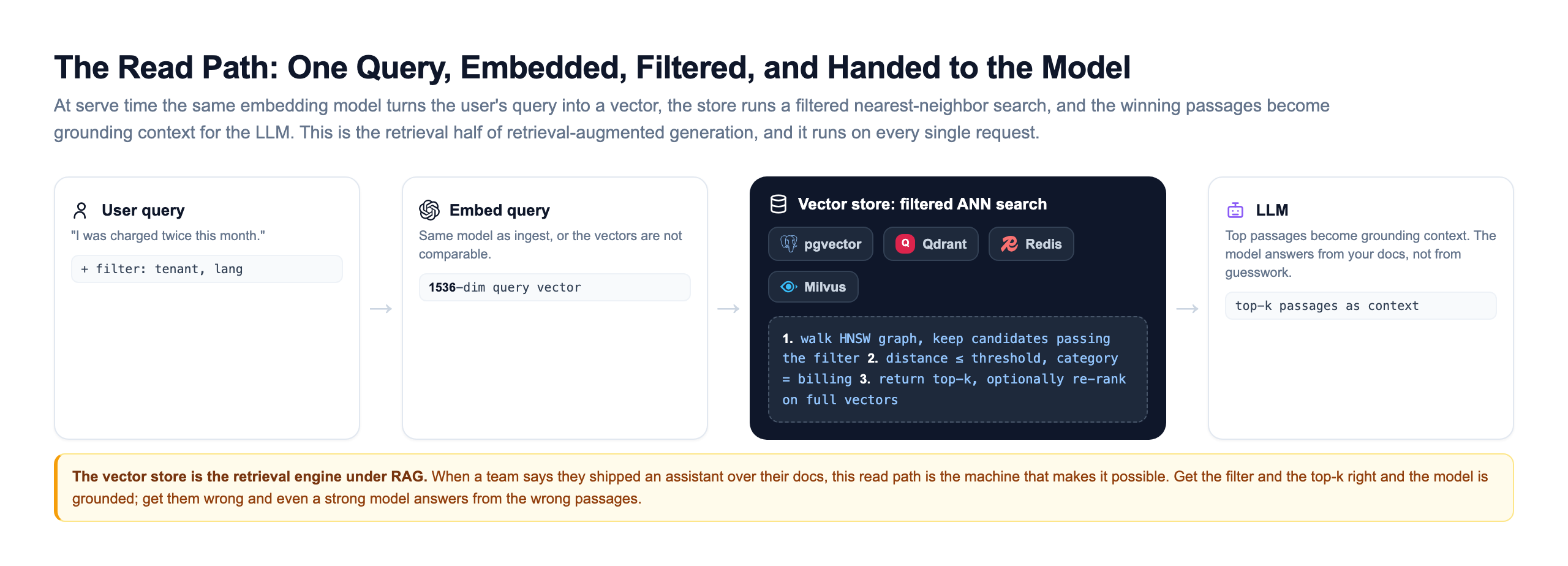
Pure nearest-neighbor search is almost never what you actually want. You want the nearest vectors that also belong to this tenant, this language, this category, or documents newer than last quarter. Vector search and metadata filtering have to happen together, and the order matters more than it looks.
The naive approach is a trap. If you fetch the top 20 by distance and then filter, you can end up with 2 results, because 18 of the nearest happened to be the wrong category. A real pushes the filter into the search so it keeps walking the graph until it has enough matches that also pass the predicate.
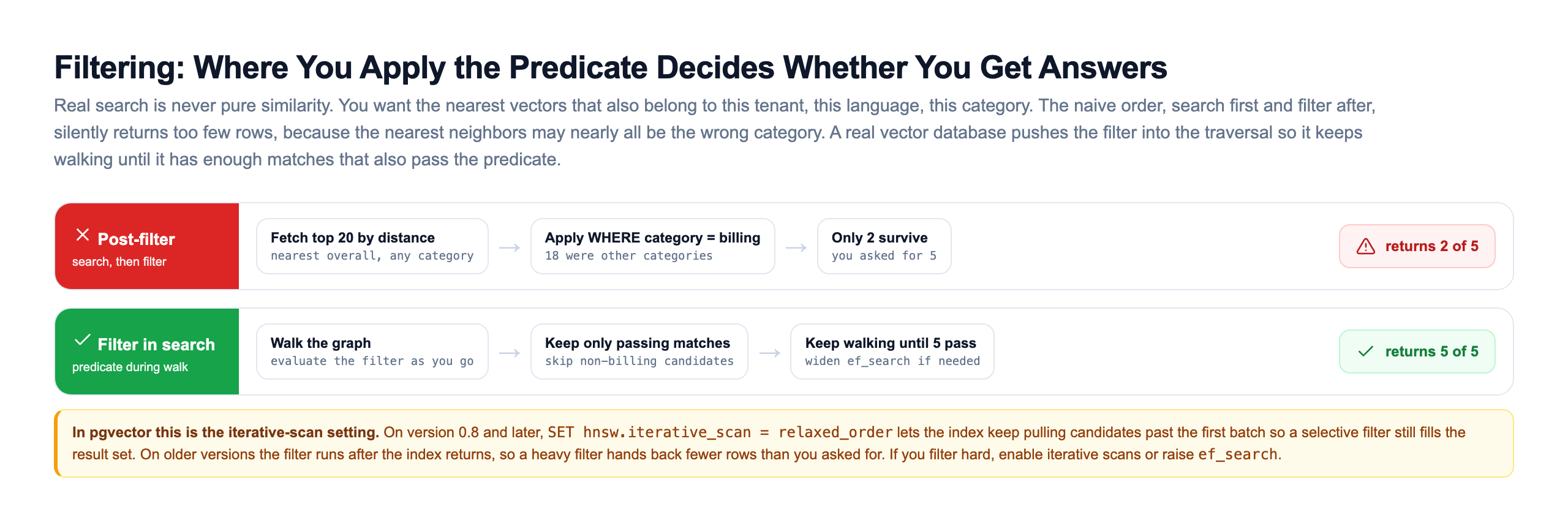
Here is the whole thing in pgvector, the Postgres extension, which is the most common starting point. You create a table with a vector column, build an index on it, then query with the distance operator and a plain SQL WHERE.
-- One-time setup
CREATE EXTENSION IF NOT EXISTS vector;

CREATE TABLE documents (
  id        bigserial PRIMARY KEY,
  content   text,
  category  text,
  embedding vector(1536)          -- one column holds the whole vector
);

-- Build an HNSW index for cosine distance.
-- m = links per node, ef_construction = build-time search width.
CREATE INDEX ON documents
  USING hnsw (embedding vector_cosine_ops)
  WITH (m = 16, ef_construction = 64);

-- Per-connection: how hard to search. This is the recall/latency knob.
SET hnsw.ef_search = 40;

-- Query: 5 nearest neighbors to the query embedding,
-- restricted to the 'billing' category. `<=>` is cosine distance.
SELECT id, content, embedding <=> $1 AS distance
FROM documents
WHERE category = 'billing'
ORDER BY embedding <=> $1
LIMIT 5;
Scaling: Why a Vector Index Shards Differently
One machine can hold maybe tens of millions of vectors in RAM with an graph on top. Past that you shard: split the vectors across many machines. But a vector index shards differently from a normal database, and the difference bites people who assume it works like the sharded stores they already know.
A sharded key-value store routes each key to exactly one shard, because you know the key. A vector index cannot do that, because the nearest neighbors of a query could sit on any shard. You do not know where the answer lives until you look.
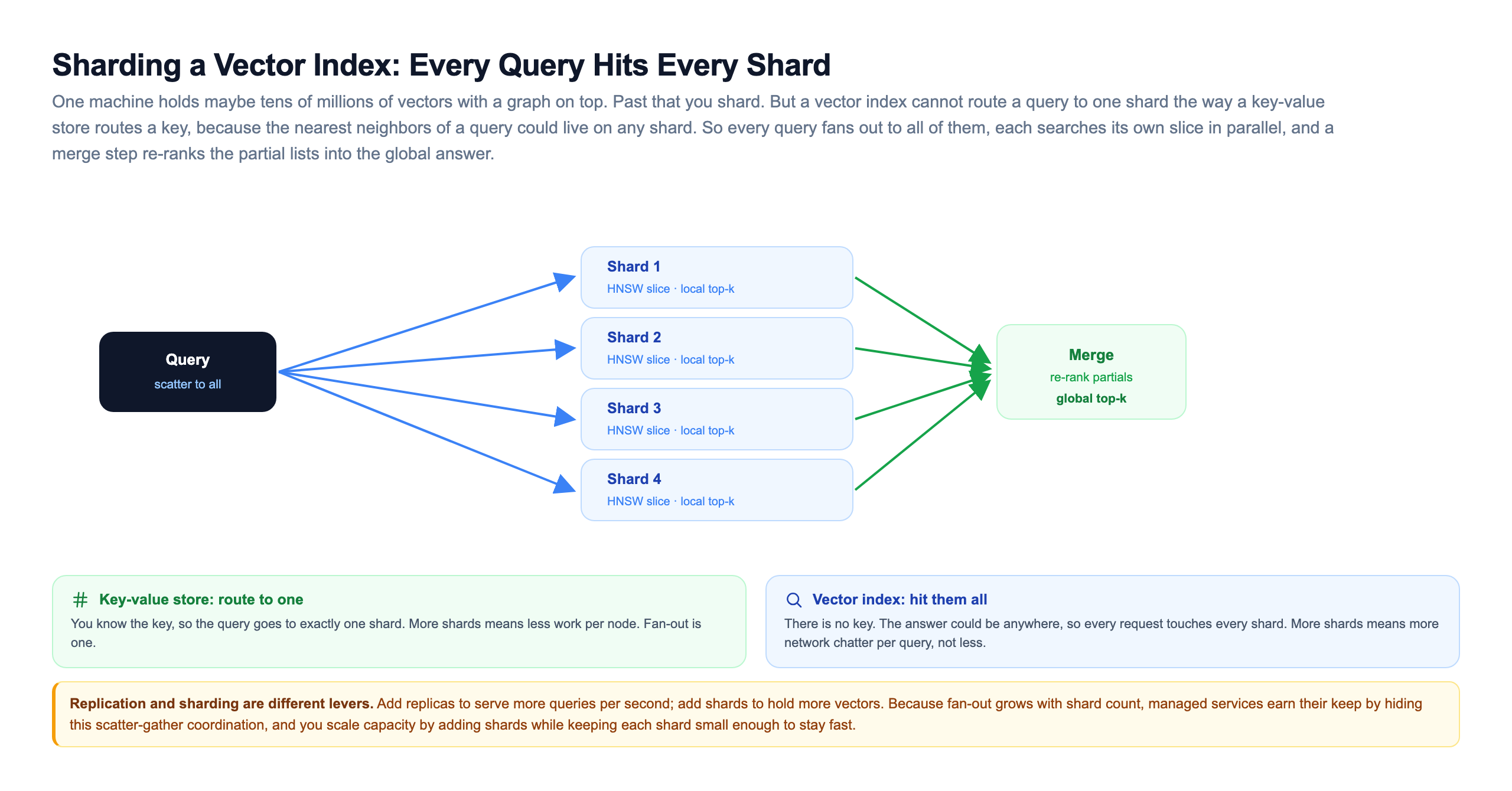
So every query fans out to every shard. Each shard searches its own slice in parallel and returns its local top-k. Then a merge step re-ranks all those partial lists into the global top-k. It stays fast because the shards work at the same time, and you scale capacity by adding shards, not by growing any one shard past the size where it stays fast.
The trade-off is fan-out. Every request hits every shard, so more shards means more network coordination per query. That is the opposite of a key-value store, where more shards means less work per node. It is why replication and are separate levers: add replicas to serve more queries per second, add shards to hold more vectors. And it is why managed vector services earn their keep, because hiding this scatter-gather coordination, the fan-out, the parallel search, the merge, is most of what they do for you.
Which Vector Database Should You Actually Use?
The market splits several ways, and the right answer depends far more on what you already run than on benchmark charts. Walk the questions and stop at the first yes.
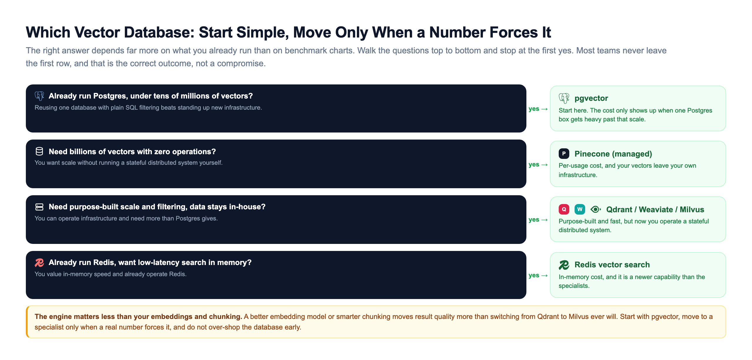
| Option | Best when | The cost |
|---|---|---|
| pgvector | You already run Postgres and are under roughly tens of millions of vectors | Scaling one Postgres box past that gets heavy |
| Pinecone (managed) | You want billions of vectors with zero operations | Per-usage cost, and your vectors leave your own infrastructure |
| Qdrant / Weaviate / Milvus (self-hosted) | You need purpose-built scale and filtering but must keep data in-house | You now operate a stateful distributed system |
| (with vector search) |
How This Runs at Scale
None of this is theoretical. Vector search is load-bearing infrastructure at the companies you use every day.
Spotify open-sourced Annoy (Approximate Nearest Neighbors Oh Yeah), one of the early ANN libraries, to power music recommendations. Finding songs similar to what you are listening to is a nearest-neighbor query over track , run millions of times a day.
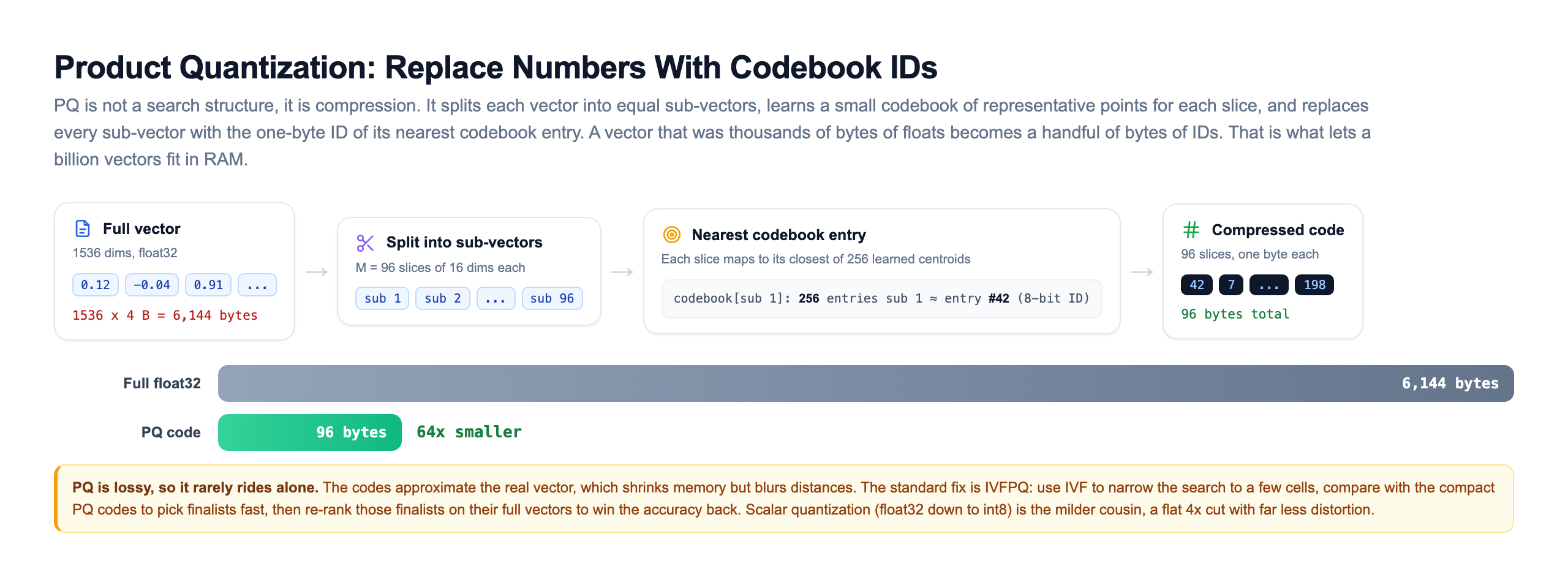
Meta built and open-sourced FAISS, the library that a huge share of the industry's ANN work sits on. FAISS is where IVF and product got battle-tested at billion-vector scale, and many vector databases use it or its ideas under the hood. When you read about IVFPQ in a managed service's docs, you are usually reading about ideas FAISS made practical.
Doordash and countless others use embeddings plus ANN search for retrieval in recommendations and search ranking, matching queries and users to items by meaning rather than exact terms.
And the entire current wave of systems, the pattern where an LLM answers from your documents instead of guessing, is a doing filtered nearest-neighbor search on every single request, then handing the winning passages to the model as grounding context. The vector index is the retrieval half of retrieval-augmented generation. When people say a company shipped an AI assistant over their docs, this is the machine that makes it possible.
The takeaway: embeddings turn meaning into geometry, ANN turns that geometry into a search you can serve in milliseconds, and a vector database is the production system that runs it under real load with real filters. Get this layer right, the chunking, the embedding model, the index type, the recall knob, the filter placement, and everything you build on top of an LLM gets more accurate and more trustworthy. Get it wrong and even the strongest model answers from the wrong passages, confidently.
Knowledge Check
Knowledge Check
4 questions - Score 80% to pass
Why is exact (brute-force) nearest-neighbor search impractical for a corpus of 100 million vectors?
In the recall/latency trade-off of ANN search, what does 'recall' measure?
You fetch the top 20 vectors by distance and then apply WHERE category = 'billing', but get back only 2 rows when you needed 5. What is the fix?
Why must a query fan out to every shard in a sharded vector index, unlike a sharded key-value store?