The Model Predicts in 8 Milliseconds. The Endpoint Falls Over at 200 Requests.
A team ships a recommendation model. In the notebook, model.predict(x) returns in 8 milliseconds and everyone is thrilled. They wrap it in a quick Flask app, put it behind a URL, and point the app at it. It works in the demo. It works for the first ten users.
Then a marketing push sends real traffic, and at a couple hundred requests per second the endpoint starts timing out. The GPU sits at 12 percent utilization while requests pile up in a queue. that was 8 milliseconds in the notebook is now 4 seconds and climbing. Nothing is technically broken. The model is fine. The serving is not.
This is the gap between a model that predicts and a model that serves. Predicting is a function call. Serving is a service that has to answer thousands of callers at once, hold a latency budget, use an expensive GPU efficiently, survive a replica crashing, roll out new versions safely, and scale when a spike hits. That is a real distributed systems problem, and it is the subject of this lesson.
A model file answers one caller. A serving system answers ten thousand callers at once, fast, without wasting the GPU, and keeps answering when a machine dies.
By the end you will understand the modes of serving, the exact path a request takes, how to pick REST or , why dynamic batching is the trick that makes GPU serving affordable, how autoscaling and cold starts interact, why the p99 latency is the number that decides if your service is good, and how to ship a new model version without betting all your traffic on it.
Three Ways to Serve, and the One Question That Decides
Before any code, get the biggest decision right. Serving splits by one question: is a user or a live flow waiting for this specific prediction right now?
If yes, you need online serving (also called real-time serving). A request comes in, and something is blocked until you answer. A fraud check on a card swipe. A search ranking. The recommendation row that has to render before the app feels ready. Here, is everything. An answer that arrives a second late is worthless even if it is correct.
If no, you need batch serving (also called offline serving). A scheduled job scores an enormous set of rows in one run, and no single row is on a clock. Precomputing recommendations for every user overnight. Scoring all accounts for churn once a week. a whole document corpus. Here, per-row latency does not matter at all. What matters is total throughput: finishing the whole run before the deadline as cheaply as possible.
There is a third shape that sits between them. Streaming serving scores an unbounded, never-ending flow of events, one window at a time, and the goal is to keep up with the arrival rate forever rather than to finish a fixed set. Live anomaly detection on a metrics firehose and scoring a clickstream as it lands are streaming problems.
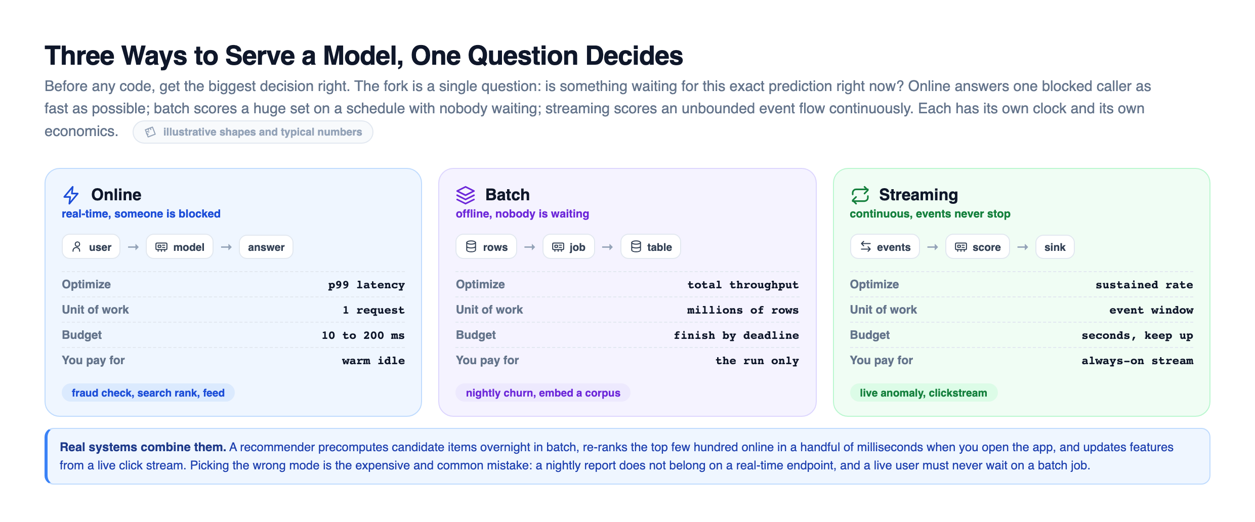
The modes have opposite economics. Online serving keeps replicas warm and idle-ready, so you pay for availability. Batch serving spins compute up, saturates it, and tears it down, so you pay only for the run. Streaming holds a long-lived job open and pays to stay caught up. Many real systems use all three: a recommender precomputes candidate items overnight in batch, re-ranks the top few hundred online in a handful of milliseconds when you open the app, and refreshes features from a live click stream in between. Picking the wrong mode is an expensive and common mistake. A nightly report does not belong on a real-time endpoint, and a live user does not belong waiting on a batch job. The rest of this lesson lives inside online serving, because that is where the hard engineering is.
The Request Path: What Actually Happens Between Click and Answer
Zoom into online serving. A prediction request does not go straight to the model. It travels through a small system, and every hop earns its place.
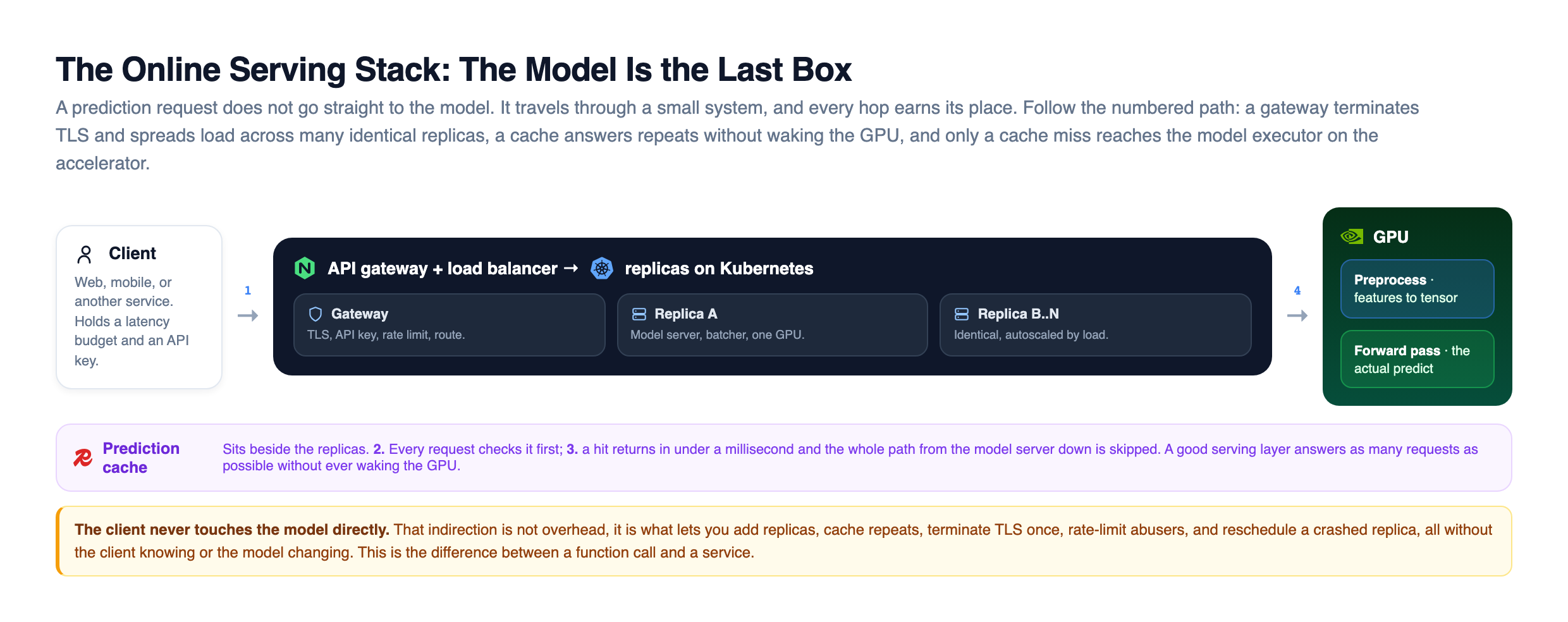
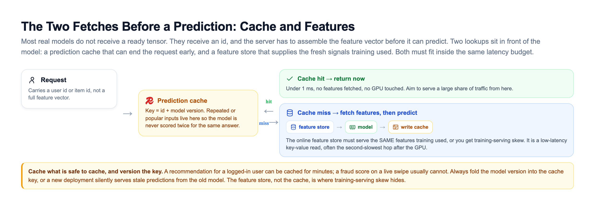
The client never touches the model server directly. In front sits an (often NGINX or a cloud ) that terminates TLS, checks the API key, applies rate limits, and spreads traffic across many identical model server replicas. A prediction cache (usually ) sits alongside so a repeated input can skip the model entirely. The model servers run on , which adds and removes replicas as load moves and reschedules any replica that crashes. The model itself runs its forward pass on a GPU. That indirection is not overhead. It is exactly what lets you add replicas, cache repeats, terminate TLS once, rate-limit abusers, and reschedule a crashed pod, all without the client knowing or the model changing.
Now walk a single request through, arrow by arrow, and watch where the time actually goes.
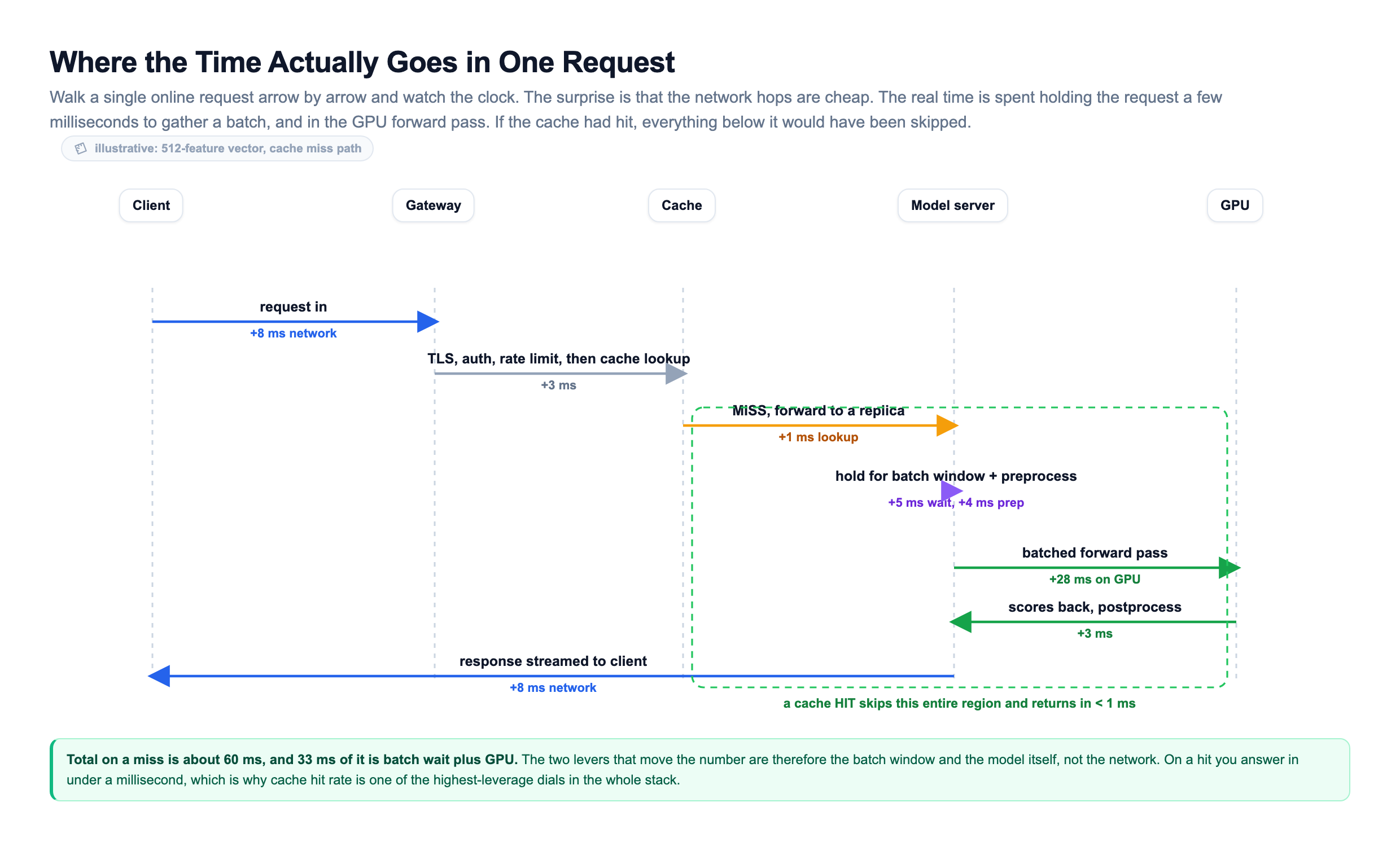
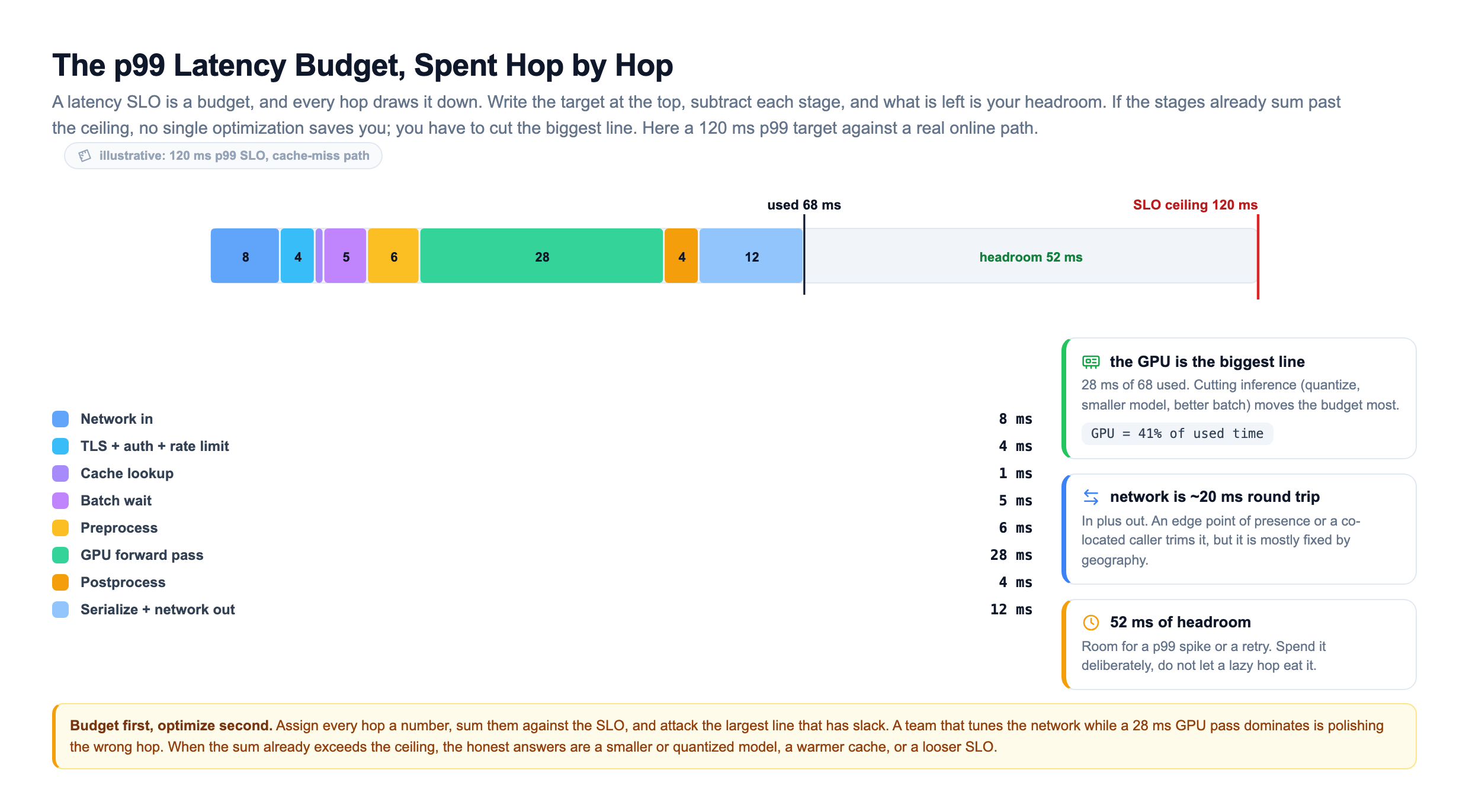
Notice the surprise: the network hops are cheap. The real time is spent in two places. First, the server deliberately holds the request for a few milliseconds to gather a batch (more on that soon). Second, the GPU forward pass. And notice the escape hatch: if the cache check had been a hit, the whole path from the model server down would have been skipped and the answer would have come back in under a millisecond. A good serving layer answers as many requests as possible without ever waking the GPU.
How the Client Talks to the Model: Protocol and Timing
The client and the model server need a shared language, and they need to agree on how long the caller can wait. Two decisions, both about who is calling and how hard.
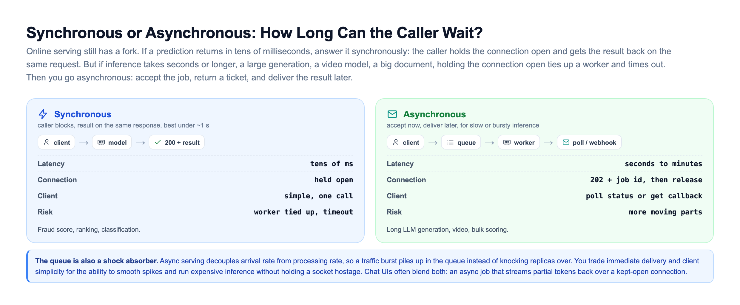
Start with the wire protocol. REST with JSON over is the default. You can curl it, read it in a browser, and debug it in Postman. JSON is text, though, so numbers become strings, keys repeat on every row, and a large feature vector or an image balloons on the wire and burns CPU to parse on both ends. with Protobuf over HTTP/2 is the high-performance option. The payload is compact binary defined by a typed .proto schema that both sides compile, a float is 4 bytes instead of a string, and many calls multiplex over one connection.
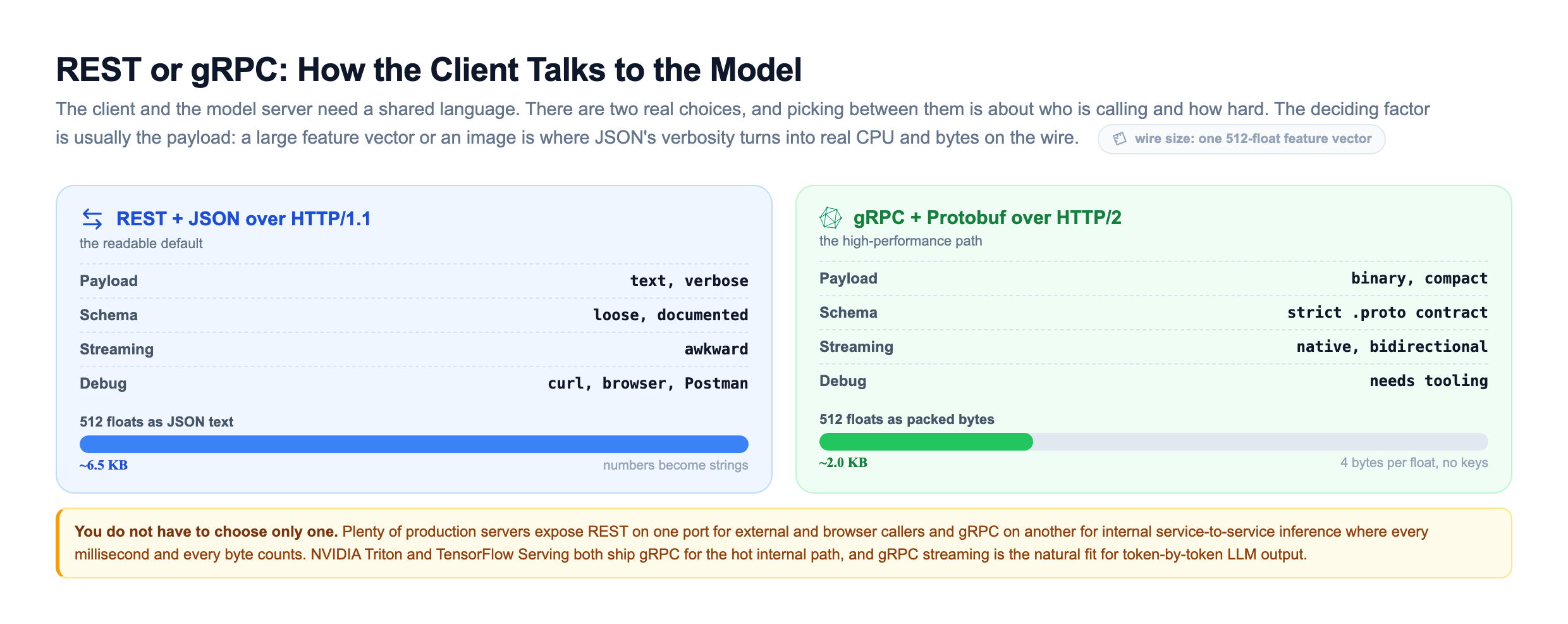
| Dimension | REST / JSON | gRPC / Protobuf |
|---|---|---|
| Payload | Text, verbose | Binary, compact |
| Transport | HTTP/1.1 |
Dynamic Batching: The Trick That Makes GPUs Affordable
Here is the single most important idea in GPU serving. A GPU running a batch of 32 inputs takes almost the same wall-clock time as running a single input, because it does the math in parallel. So if you feed the GPU one request at a time, it sits nearly idle between requests and you pay a fortune per prediction. If you feed it full batches, you get many predictions for roughly the cost of one.
But in online serving, requests arrive one at a time from different users. You cannot ask users to show up in neat groups of 32. Dynamic batching solves this: the server holds each incoming request for a tiny, bounded window (say up to 5 milliseconds), gathers whatever other requests arrive during that window, and runs them all as one batch.
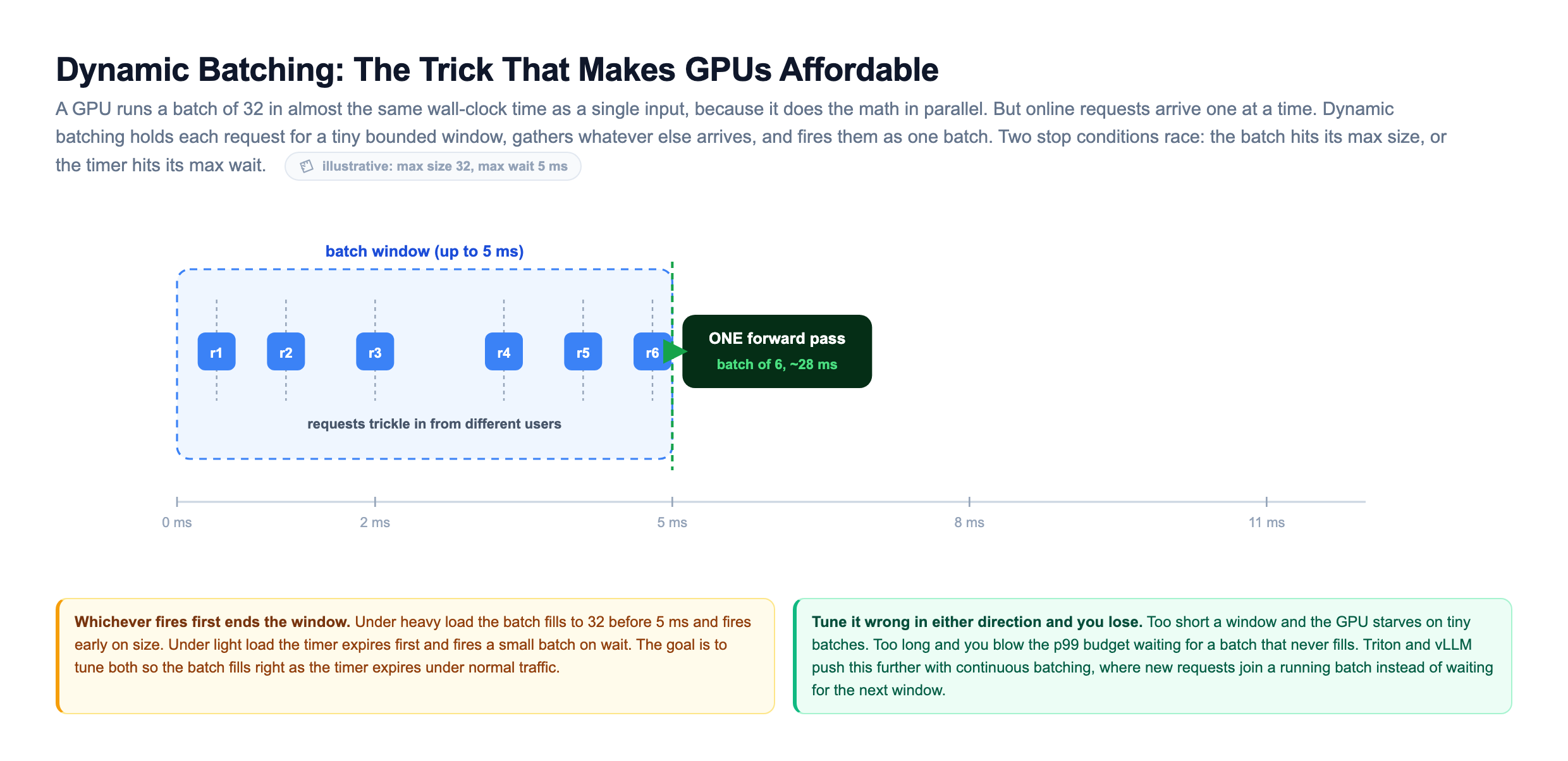
The window has two stop conditions racing each other: the batch hits its max size, or the timer hits its max wait. Whichever comes first ends the window and fires the forward pass. This is a direct trade: you spend a few milliseconds of latency to buy several times the throughput. Tune it wrong in either direction and you lose. Too short a window and the GPU starves on tiny batches. Too long and you blow your p99 latency budget waiting for a batch that never fills. The goal is to set max batch size and max wait so the batch fills right as the timer expires under normal load. Triton and vLLM push this further with , where new requests join a running batch instead of waiting for the next window, which is a big deal for LLMs where one generation can take seconds.
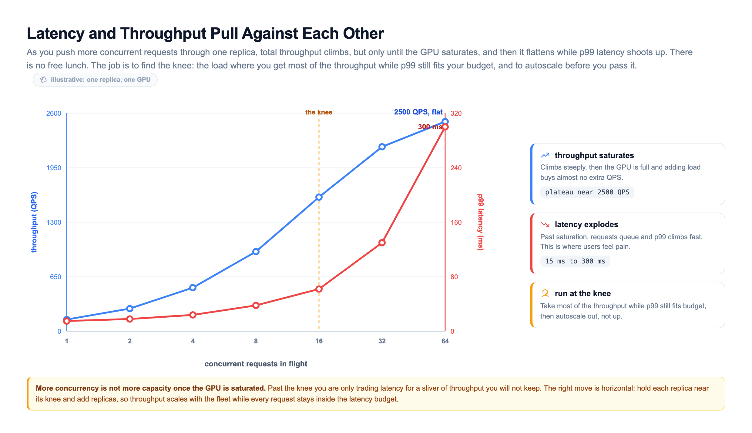
Batching is not a free lever, though. It sets the position on a curve that every serving engineer has to understand: as you push more concurrent requests through one replica, total throughput climbs, but only until the GPU saturates, after which throughput flattens while explodes.
A Real Serving Endpoint, and a Batching Simulator You Can Run
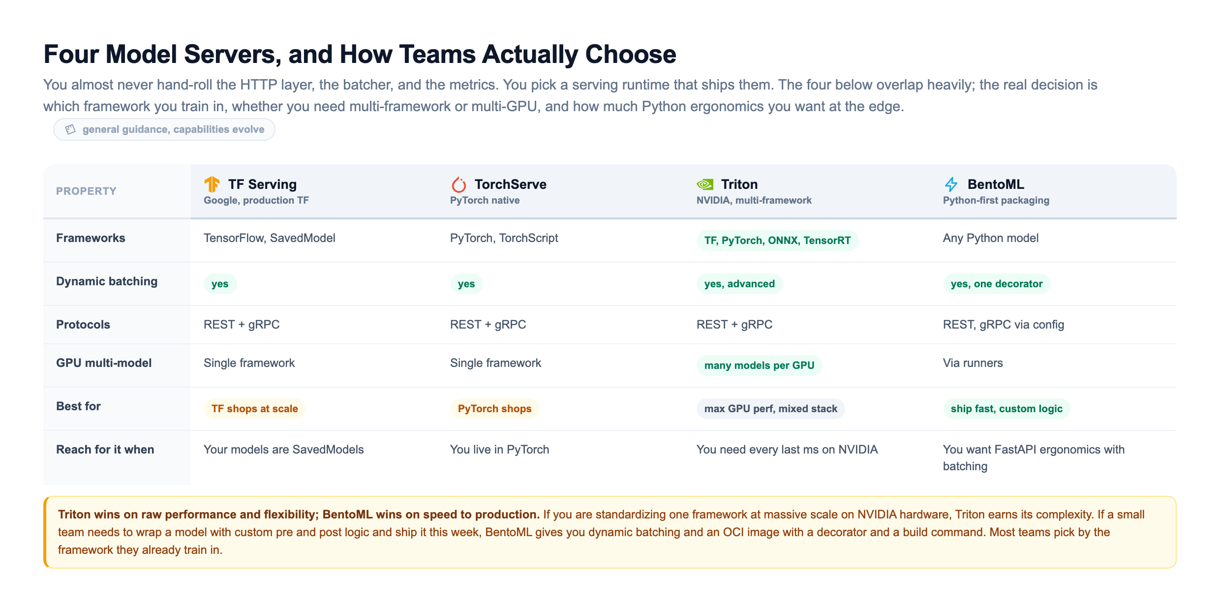
Enough theory. Here is a real online serving endpoint. BentoML is a serving framework that wraps your model in a service, handles the layer, and gives you dynamic batching with a single decorator argument. This is a recommendation ranking service that scores candidate items for a user.
import bentoml
import numpy as np
import torch


@bentoml.service(
    resources={"gpu": 1},          # this service needs one GPU
    traffic={"timeout": 10},        # reject any request still open after 10s
    workers=1,                      # one worker owns the GPU; scale with replicas
)
class RecommenderService:
    def __init__(self) -> None:
        # Loaded ONCE at startup, then kept warm in GPU memory.
        # This is the cold start: heavy now, so every request stays cheap.
        self.model = torch.jit.load("ranking_model.pt")
        self.model.eval()
        self.model.to("cuda")

    @bentoml.api(
        batchable=True,             # let BentoML batch concurrent calls
        batch_dim=0,                # stack requests along axis 0
        max_batch_size=32,          # never build a batch bigger than 32
        max_latency_ms=5,           # ...and never wait longer than 5ms to fill it
    )
    def rank(self, features: np.ndarray) -> np.ndarray:
        # `features` arrives already batched: shape (N, feature_dim),
        # where N is however many requests BentoML grouped this window.
        with torch.no_grad():
            x = torch.from_numpy(features).float().to("cuda")
            scores = self.model(x)                 # one forward pass, whole batch
            return scores.cpu().numpy()            # shape (N,), one score per request
Read what each part buys you. The model loads once in __init__, so the expensive weight load happens at startup, not on every request. The batchable=True plus max_batch_size and max_latency_ms give you exactly the dynamic batching from the last slide, declared in three lines. The rank method receives an already-batched array and returns one score per row, so you write the model logic once and the framework handles the fan-in and fan-out. You start this with bentoml serve, containerize it into an OCI image with , and ship that image to .
Autoscaling, Cold Starts, and Why p99 Is the Number That Matters
Traffic is never flat. It spikes at lunch, drops at 3am, and jumps when marketing sends an email. So the serving layer has to autoscale, and inference autoscaling has a nasty twist that web autoscaling does not: the cold start.
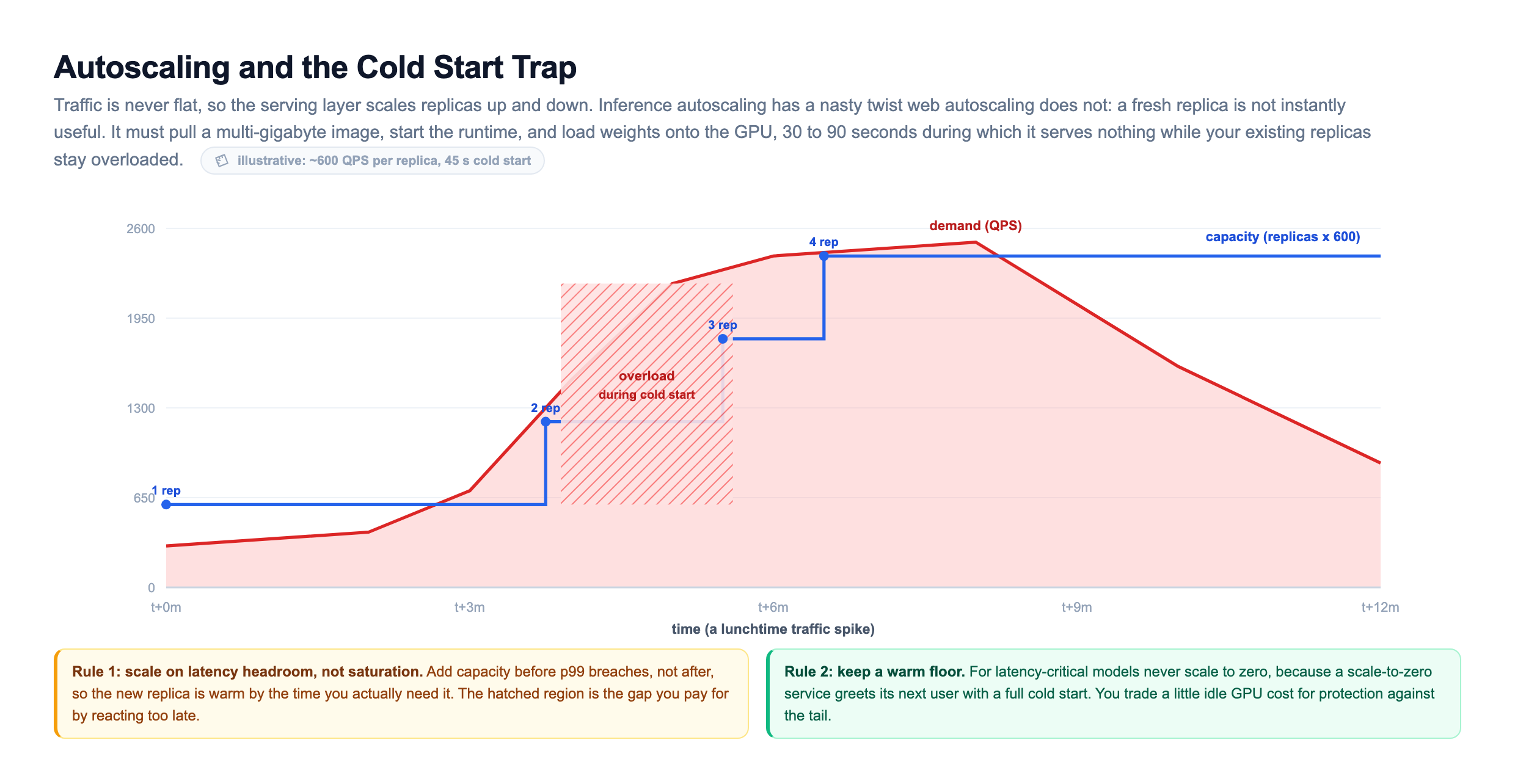
When load rises, Kubernetes adds a replica. But a fresh model server pod is not instantly useful. It has to pull a multi-gigabyte container image, start the runtime, and load model weights onto the GPU. For a large model that is 30 to 90 seconds during which the new replica serves nothing while your existing replicas stay overloaded. That overload window is the hatched region in the figure, and it is you pay for by reacting too late. Two rules follow. First, scale on latency headroom, not on saturation, so you add capacity before p99 breaches, not after. Second, keep a warm floor: for latency-critical models you never scale to zero, because a scale-to-zero service greets its next user with a cold start. You trade a little idle GPU cost for protection against tail latency.
That word tail is the whole point. Serving quality is not measured by the average latency, it is measured by the tail: p50, p95, p99. Here is why the average lies.
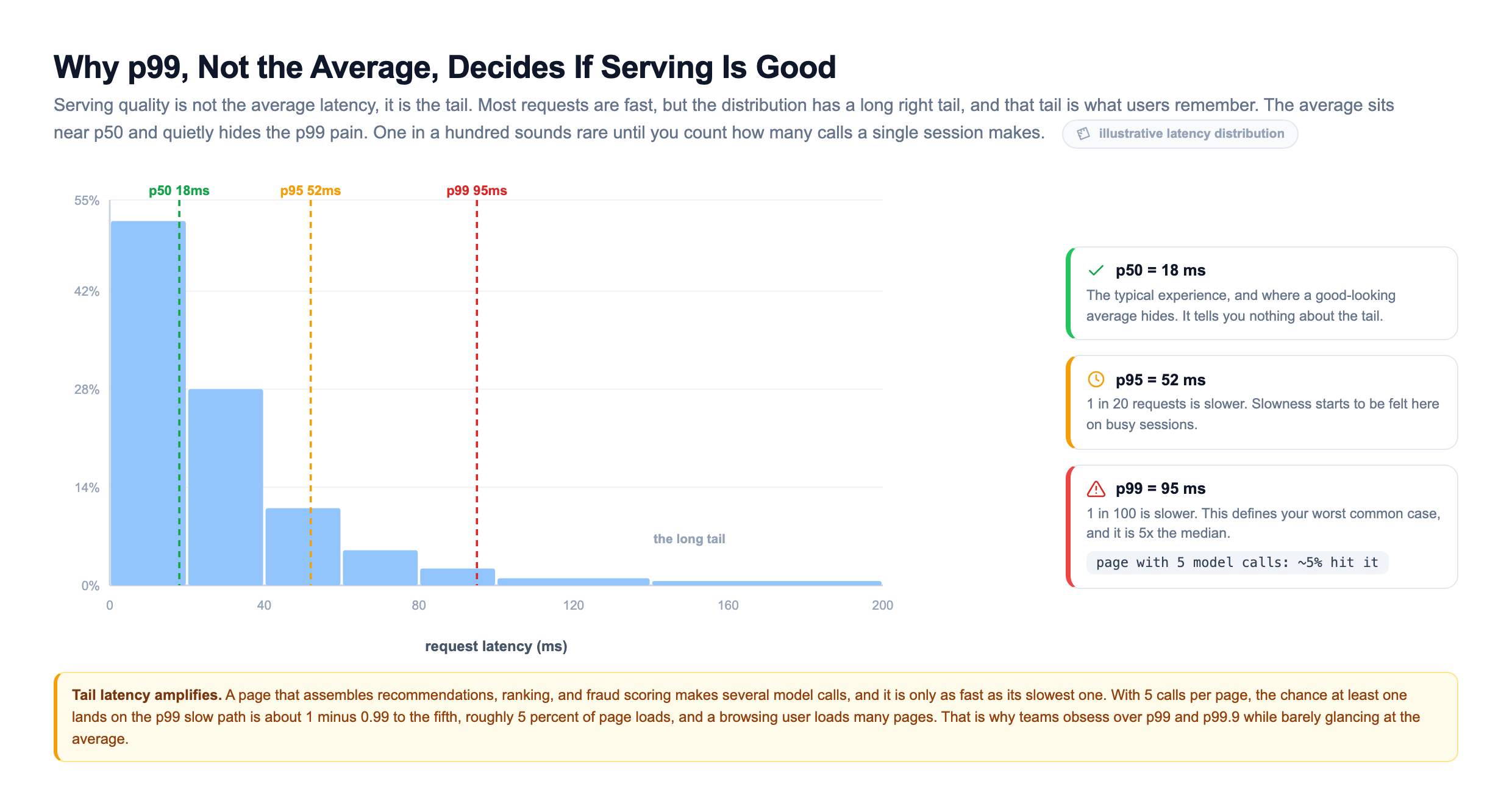
| Metric |
|---|
Shipping a New Version Without Betting All Your Traffic
The last piece of serving is not about a single request, it is about change. A model that predicts well on your offline test set can still fail in production: the live feature distribution has drifted, a dependency added , an edge case crashes the new code path. You never cut all traffic from the old model to a new one in a single switch. Two patterns let live traffic vet a candidate before it owns the request.
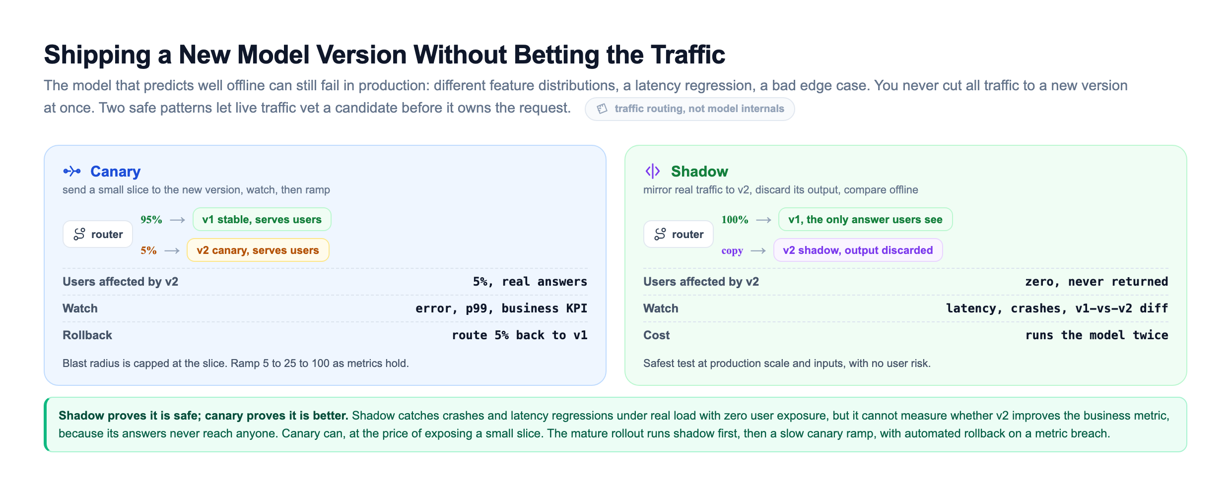
Canary routes a small slice of real traffic, say 5 percent, to the new version while the rest stays on the stable one. Real users get v2 answers, so you can measure not just whether it stays up but whether it actually improves the metric you care about. You watch error rate, p99, and the business KPI on the canary slice, and if anything degrades you route the slice back to the stable version. The blast radius is capped at the slice, and you ramp 5 to 25 to 100 percent as the metrics hold.
Shadow (also called dark launch) mirrors real production traffic to the new version but throws its answers away. Users only ever see the stable version's output. The shadow copy runs against real inputs at real scale, so you catch crashes, latency regressions, and behavior differences with zero user exposure. The cost is running the model twice for the shadowed traffic.
Shadow proves it is safe; canary proves it is better. Shadow catches crashes and latency regressions under real load with no user risk, but because its answers never reach anyone, it cannot tell you whether v2 improves the business metric. Canary can, at the price of exposing a small slice. The mature rollout runs shadow first to catch the obvious failures, then a slow canary ramp with automated rollback wired to a metric breach. This is also why the cache key and every logged prediction carry the model version: when two versions run at once, you need to know which one produced any given answer.
How the Giants Serve at Scale
None of this is hypothetical. Every company running ML at scale hit these exact problems and built exactly this kind of serving layer.
DoorDash serves ranking and recommendation models on every home screen and search. To hold at high request rates, they moved heavy prediction traffic onto a dedicated prediction service and leaned hard on feature caching and request batching so a GPU is never scored one order at a time. The pattern is the one in this lesson: gateway, cache, batched model servers, autoscaled behind a latency budget.
Netflix ranks the rows you see with models that must respond in tens of milliseconds while a page assembles. They precompute heavy candidate generation offline in batch, then do the fast, personalized re-ranking online, which is the batch-then-online split from the second slide made real.
Spotify built its serving on top of and standard model servers so that hundreds of models, from Discover Weekly to the home feed, share one autoscaling, monitored serving substrate instead of each team hand-rolling a Flask app. That shared substrate is also what makes canary and shadow rollouts a standard, safe operation rather than a bespoke risk for every team.
For large language models, the shape shifts but the ideas hold. vLLM and NVIDIA Triton are the workhorses, and their headline feature is , the same latency-for-throughput trade you saw, tuned for generation where each request produces tokens over seconds. Companies serving LLM features route requests through vLLM precisely so one expensive GPU serves many concurrent conversations at once, and they stream tokens back over async connections because a full generation is far too slow for a synchronous call. Same lesson, bigger model: turning a model file into a service that survives real traffic is its own engineering discipline, and now you know its moving parts.
Knowledge Check
Knowledge Check
4 questions - Score 80% to pass
A nightly job scores every user for churn risk and writes the results to a table. No user is waiting on any single prediction. Which serving mode fits?
Why does dynamic batching improve GPU serving?
Why do serving teams obsess over p99 latency instead of the average?
You want to ship model v2, but you are not sure it stays up under real load. Which rollout catches crashes and latency regressions with zero user exposure?