How Models Generate

What a Long Prompt Really Costs: Wait, Writing Speed and Memory

0 of 20 complete

0%

Contents

Back|How Models GenerateWhat a Long Prompt Really Costs: Wait, Writing Speed and Memory
1/20
45 min left

Why Not Just Send Everything?

When you build with a language model, it is tempting to put everything into the prompt: the whole document, the whole chat history, every rule you can think of. More context sounds safer. But a prompt is not free. Something has to read it, keep it, and look back at it while writing.

Think of a librarian asked a question. If you hand over one page, the answer comes quickly. If you hand over a whole shelf of books, the librarian has to read the shelf before saying anything, and then keep glancing back at it while answering.
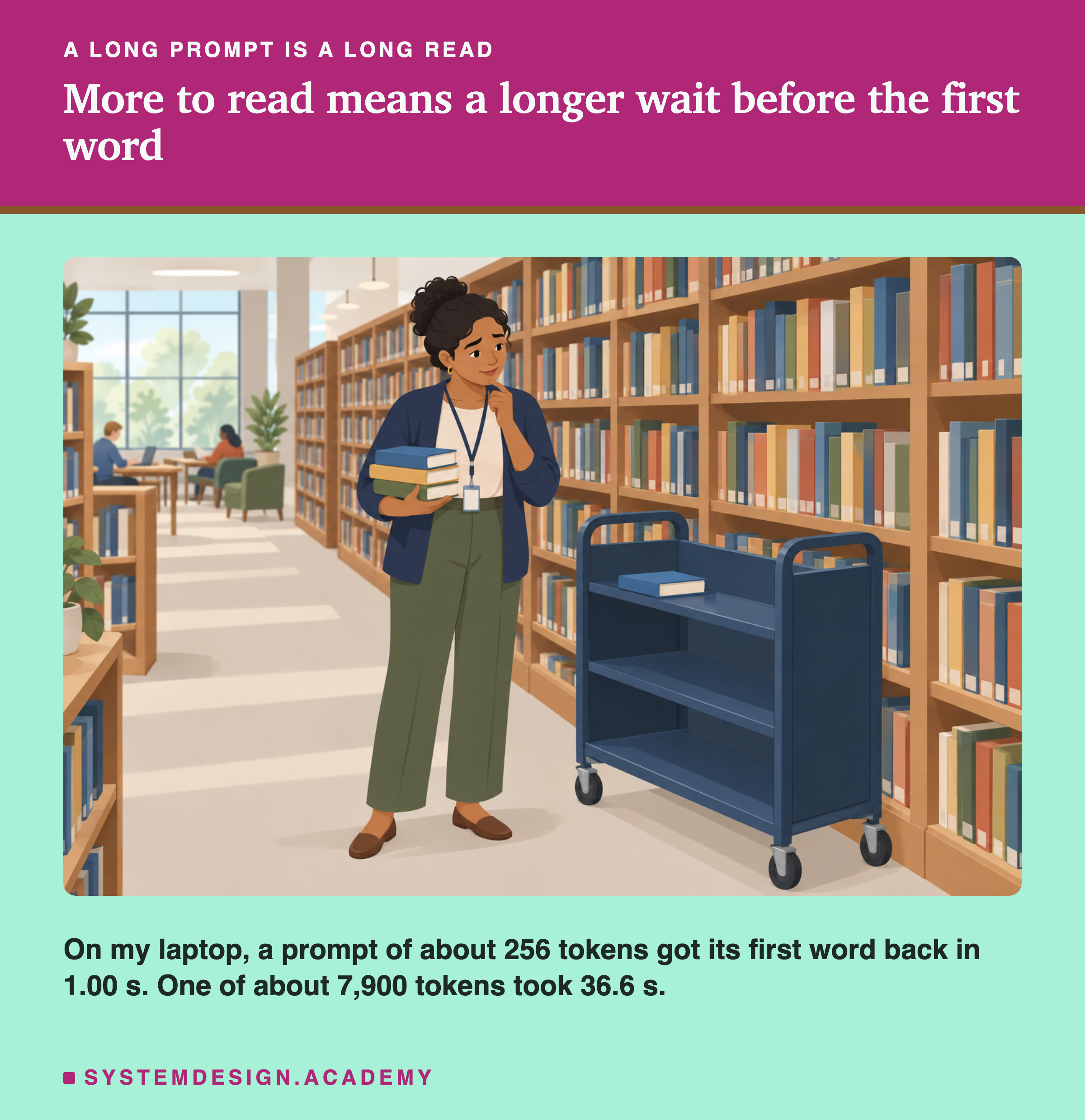
An illustration of a library scene. Beneath: on my laptop, a prompt of about 256 tokens got its first word back in 1.00 s, and one of about 7,900 tokens took 36.6 s.

This lesson measures three costs of a long prompt on my laptop: how long a person waits before the first word appears, whether the writing gets slower, and how much memory the model sets aside. It also explains where each cost comes from, using the keys and values from lesson 4.

By the end you will be able to estimate the wait for a prompt of any length, work out how much memory one token's stored keys and values take, and decide when a long prompt is worth it.

Words You Need First
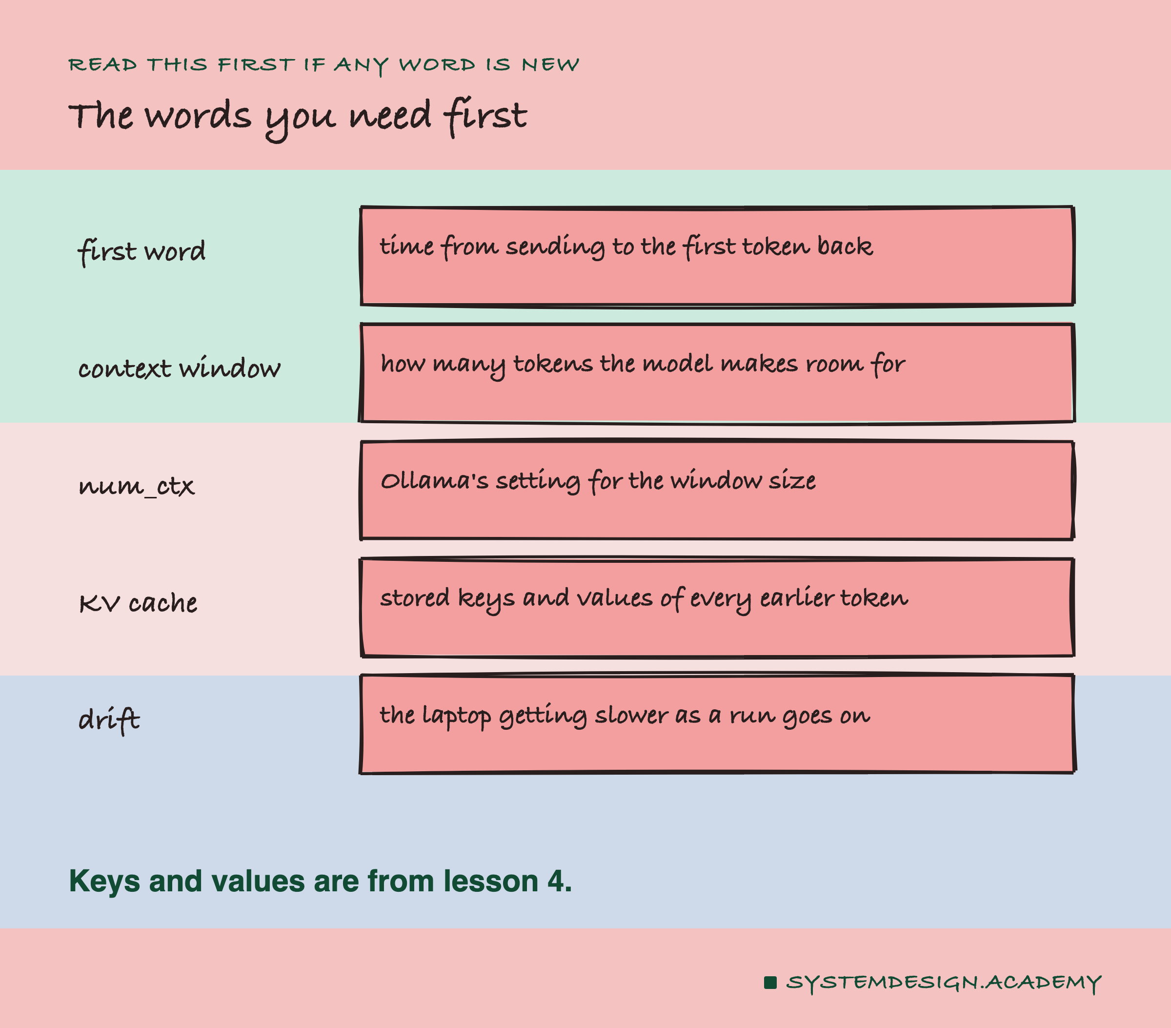
A hand-drawn list of five terms. First word: time from sending to the first token back. Context window: how many tokens the model makes room for. num_ctx: Ollama's setting for the window size. KV cache: stored keys and values of every earlier token. Drift: the laptop getting slower as a run goes on. Beneath: keys and values are from lesson 4.

Time to the first word. How long a person waits, from sending the request to seeing the first token of the reply. Engineers often call it time to first token. It is loading plus reading plus one written token.

Context window. The most tokens a model will handle in one request, prompt and reply together. Ollama calls the setting num_ctx. It is decided when the model is loaded, not when the prompt arrives.

. In lesson 4, every word had a key and a value in every layer. While the model works, it keeps those keys and values for every token it has already seen, so it never has to compute them again. That store is the KV cache, K for keys and V for values.

In lesson 3, the laptop got slower as a long run went on. That slowing is called drift here, and it matters again in this lesson.
Prerequisites
Attention: How Each Word Looks Back at the Words Before Itrequired
Related Topics
What a Token Is: How a Language Model Reads TextTokens and EmbeddingsThe Silent Cut: How Much of Your Text an Embedding Model Really ReadsTokens and EmbeddingsMCP in Production: What the Protocol Buys and CostsAgents in Production
1 of 20
Drift.

Median and range. The median is the middle value once the results are sorted. The range is the lowest and highest. This lesson reports both, because timings on a laptop move around.

The Wait Before the First Word

The first measurement is the one a person feels: how long before anything appears.

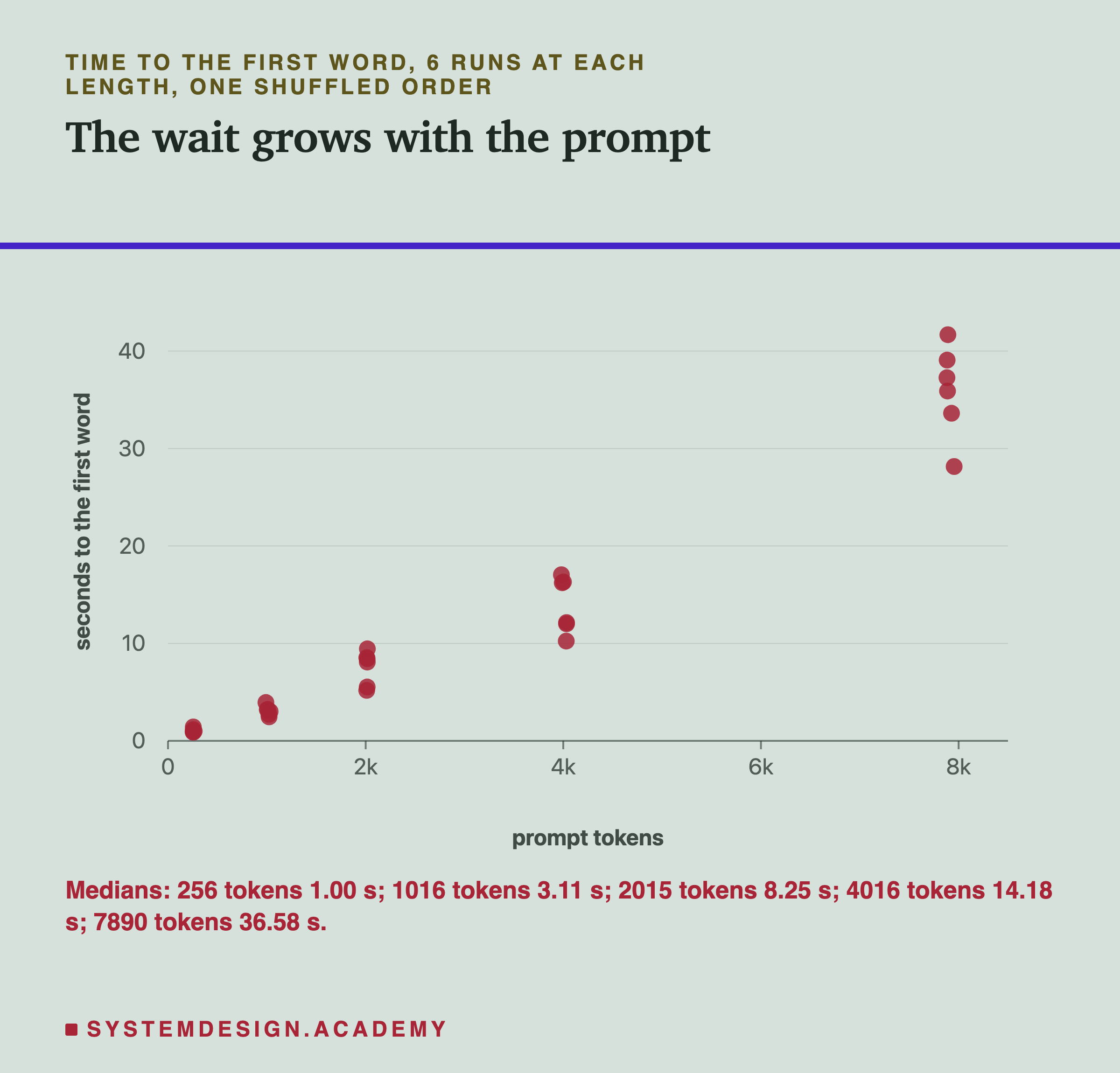
A scatter chart of seconds to the first word against prompt tokens, one dot per run, 6 runs at each of about 256, 1,016, 2,015, 4,016 and 7,890 tokens. The dots rise from about 1 second at 256 tokens to between about 28 and 42 seconds at about 7,900. Beneath: medians, 256 tokens 1.00 s; 1016 tokens 3.11 s; 2015 tokens 8.25 s; 4016 tokens 14.18 s; 7890 tokens 36.58 s.

The medians were 1.00 second for about 256 tokens, 3.11 for about 1,000, 8.25 for about 2,000, 14.18 for about 4,000 and 36.58 for about 7,900. Almost all of that is reading: the median reading time at 7,900 tokens was 36.40 seconds, and writing the first token added only a small part of a second.

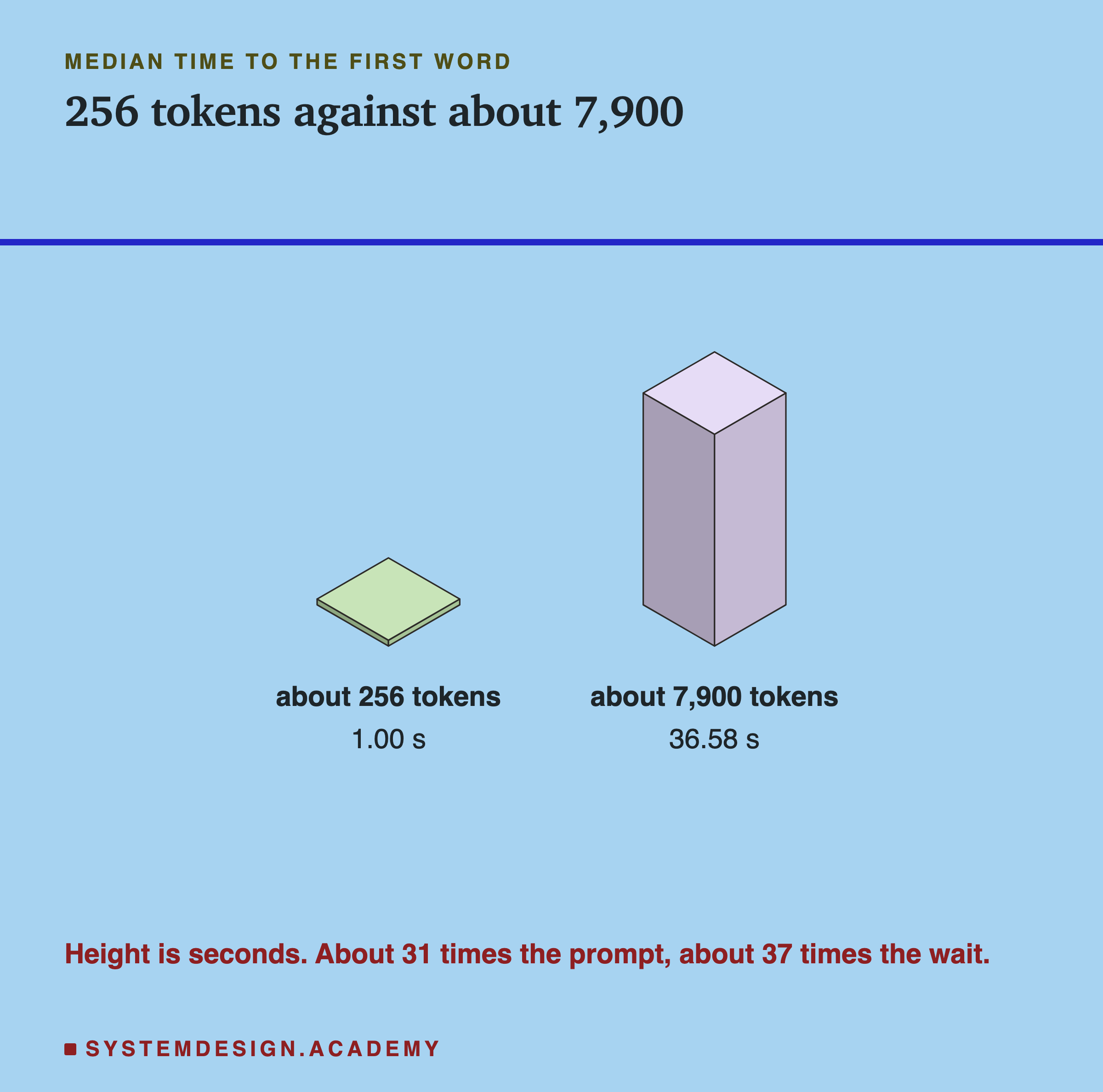
Put another way: the prompt of about 7,900 tokens was 7,890 ÷ 256 ≈ 31 times longer than the short one, and the wait was 36.58 ÷ 1.00 ≈ 37 times longer. So the wait grew a little faster than the prompt, though the laptop's drift, described below, blurs the exact shape.

Two isometric blocks, headed median time to the first word, titled 256 tokens against about 7,900. A thin flat slab, about 256 tokens, 1.00 s, beside a tall block, about 7,900 tokens, 36.58 s. Beneath: height is seconds, about 31 times the prompt, about 37 times the wait.

For a person, 1 second feels immediate and 36 seconds feels broken. That is the most important cost in this lesson.

These numbers are faster than lesson 3's, where about 4,000 tokens took about 21 seconds to read and here about 14. It was a different day and a different window size, which is why each lesson measures its own run instead of reusing another lesson's numbers.

Where the Wait Goes

Lesson 3 split every call into three parts: loading the model, reading the prompt, and writing the reply. The wait before the first word is the first two parts plus the time to write one token. So which part is it?

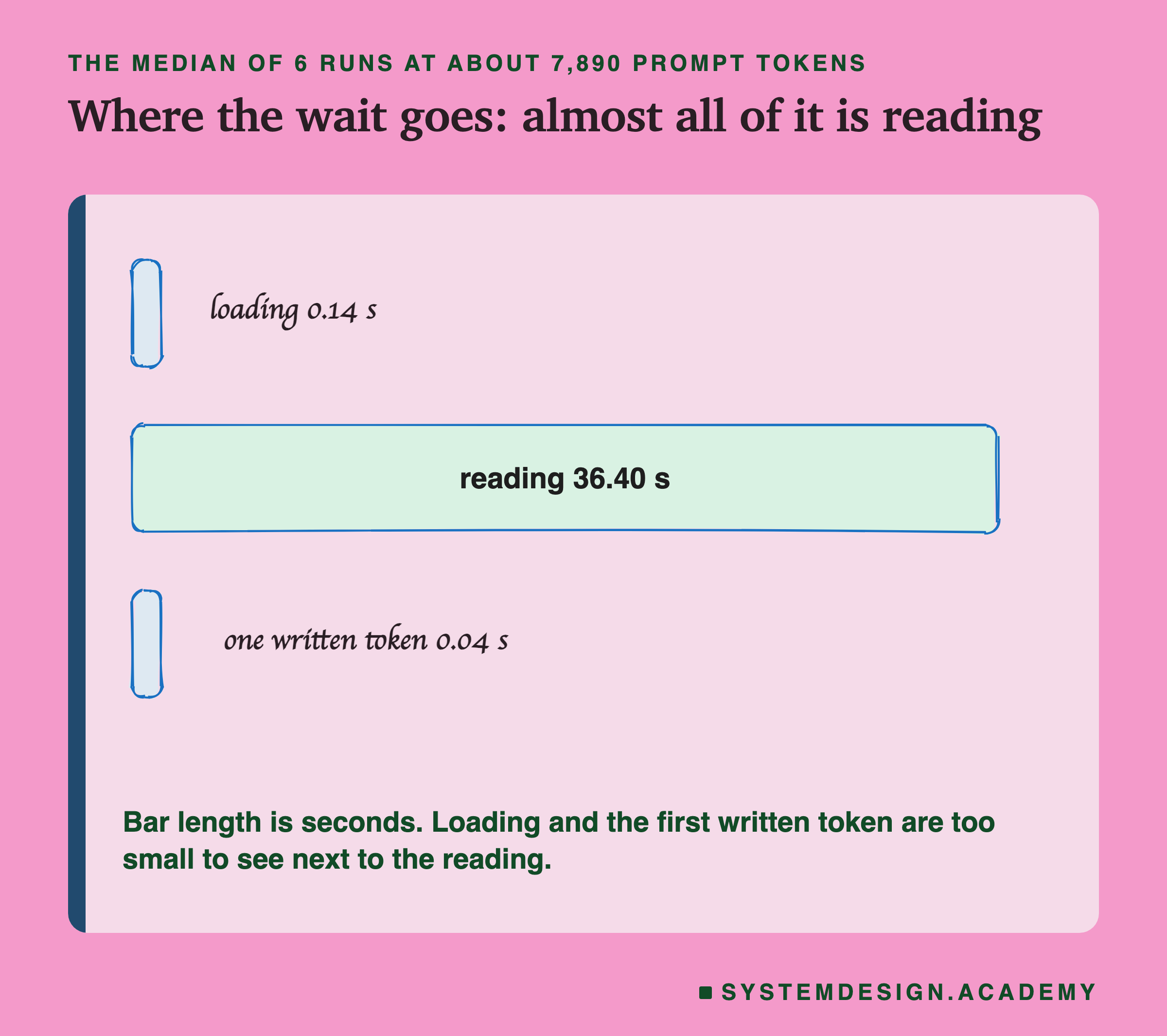
A hand-drawn bar chart headed the median of 6 runs at about 7,890 prompt tokens, titled where the wait goes, almost all of it is reading. Three bars, length in seconds: loading 0.14 s, a thin sliver; reading 36.40 s, the full width; one written token 0.04 s, a thin sliver. Beneath: bar length is seconds, and loading and the first written token are too small to see next to the reading.

For the prompts of about 7,900 tokens, the medians were 0.14 seconds of loading, 36.40 seconds of reading and 0.04 seconds for one written token. Add them up and you get about 36.6 seconds, the first-word median. Reading is 36.40 ÷ 36.58, more than 99% of the wait.

That tells you where to look for a fix. Loading was already small, because the model stayed in memory between calls; if your server unloads the model when it is idle, loading can take from under a second, when the file is still cached, to over 20 seconds on a cold start (lesson 3 measured 0.69 and 22.9), and keeping the model loaded fixes that. A faster writing speed would not help the wait at all, since only one token is written before the first word appears. The only ways to shorten this wait are to read less, to read faster on a stronger machine, or to reuse a start the model has already read, which a later lesson in this chapter does on purpose.

Reading speed on this laptop sat between about 190 and 450 tokens a second across all 30 calls. At a median of about 217 tokens a second for the longest prompts, every extra 1,000 tokens of prompt costs roughly 1,000 ÷ 217 ≈ 4.6 seconds of waiting. That rough rule, seconds of wait per 1,000 tokens, is the most useful number to take away for your own machine, and the script on the next slide measures it.

Time the First Word Yourself

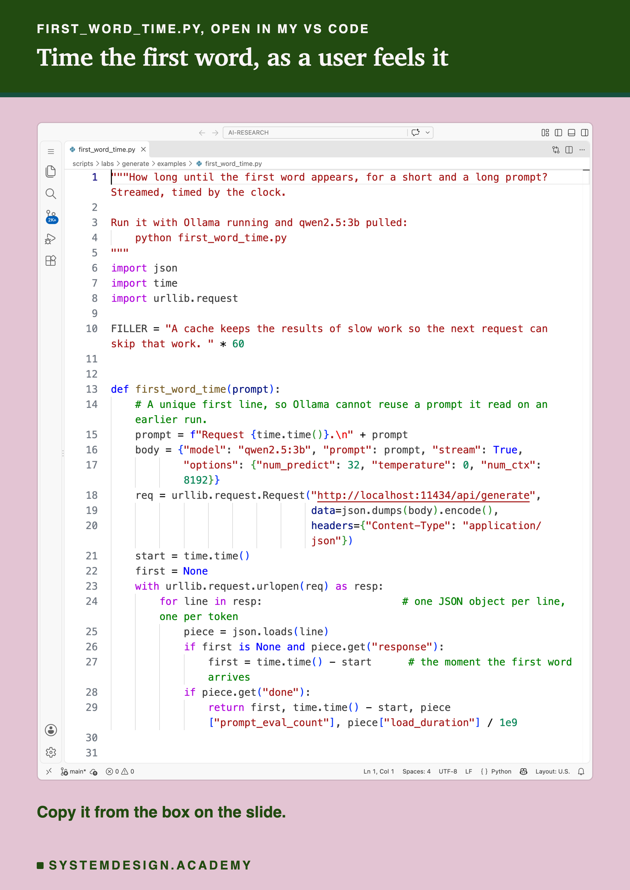
The lab did not use a clock. It computed the first-word time from Ollama's own timings, as loading plus reading plus one token's share of the writing time. This small script measures the wait the way a user feels it: it streams the reply and uses a clock to note when the first piece arrives.

A real screenshot of VS Code with first_word_time.py open. It builds a filler text, defines first_word_time, which adds a unique first line to the prompt, sends it to Ollama with stream true, reads the reply line by line, records the time when the first piece of text arrives, and returns that time with the total time, the tokens read and the load time. Beneath: copy it from the box on the slide.

"""How long until the first word appears, for a short and a long prompt? Streamed, timed by the clock.

Run it with Ollama running and qwen2.5:3b pulled:
    python first_word_time.py
"""
import json
import time
import urllib.request

FILLER = "A cache keeps the results of slow work so the next request can skip that work. " * 60


def first_word_time(prompt):
    # A unique first line, so Ollama cannot reuse a prompt it read on an earlier run.
    prompt = f"Request {time.time()}.\n" + prompt
    body = {"model": "qwen2.5:3b", "prompt": prompt, "stream": True,
            "options": {"num_predict": 32, "temperature": 0, "num_ctx": 8192}}
    req = urllib.request.Request("http://localhost:11434/api/generate",
                                 data=json.dumps(body).encode(),
                                 headers={"Content-Type": "application/json"})
    start = time.time()
    first = None
    with urllib.request.urlopen(req) as resp:
        for line in resp:                       # one JSON object per line, one per token
            piece = json.loads(line)
            if first is None and piece.get("response"):
                first = time.time() - start      # the moment the first word arrives
            if piece.get("done"):
                return first, time.time() - start, piece["prompt_eval_count"], piece["load_duration"] / 1e9


for label, prompt in [("short", "Explain in one sentence what a cache is."),
                      ("long", FILLER + "\nExplain in one sentence what a cache is.")]:
    first, total, n, load = first_word_time(prompt)
    print(f"{label:>5} prompt, {n:4d} tokens read: first word after {first:.2f} s "
          f"(of which loading {load:.2f} s), done after {total:.2f} s")

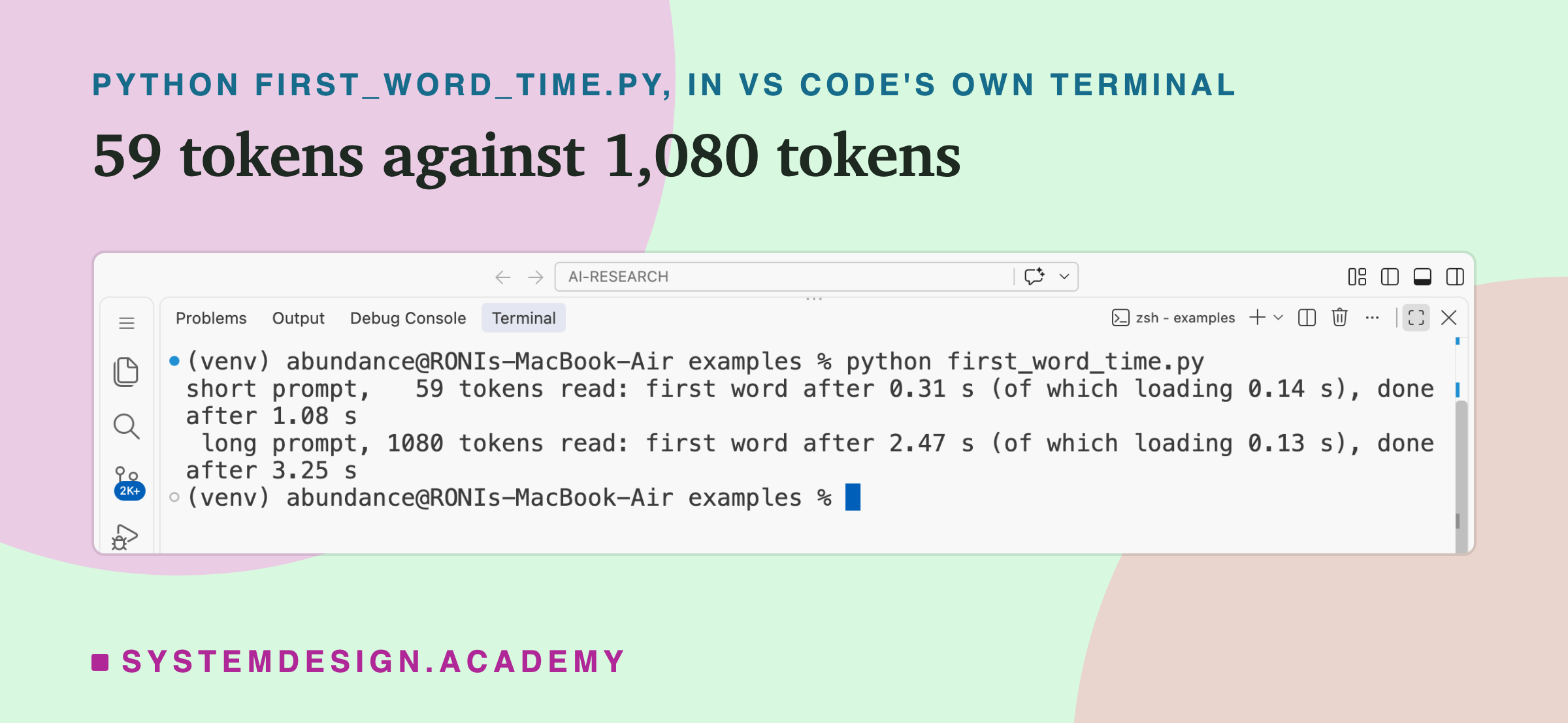
This is a real run in VS Code's terminal.

A real screenshot of VS Code's terminal after running python first_word_time.py. The short prompt, 59 tokens read: first word after 0.31 s, of which loading 0.14 s, done after 1.08 s. The long prompt, 1080 tokens read: first word after 2.47 s, of which loading 0.13 s, done after 3.25 s.

The short prompt showed its first word after 0.31 seconds. The long one, 1,080 tokens, took 2.47 seconds, about eight times as long. The load time was small in both, about 0.13 seconds, because the model was already in memory.

A Trap I Walked Into

Lesson 3 warned about this, and I still walked into it. The run you just saw is not the first one I made. My first version of the script had no unique first line, and I had run it before.

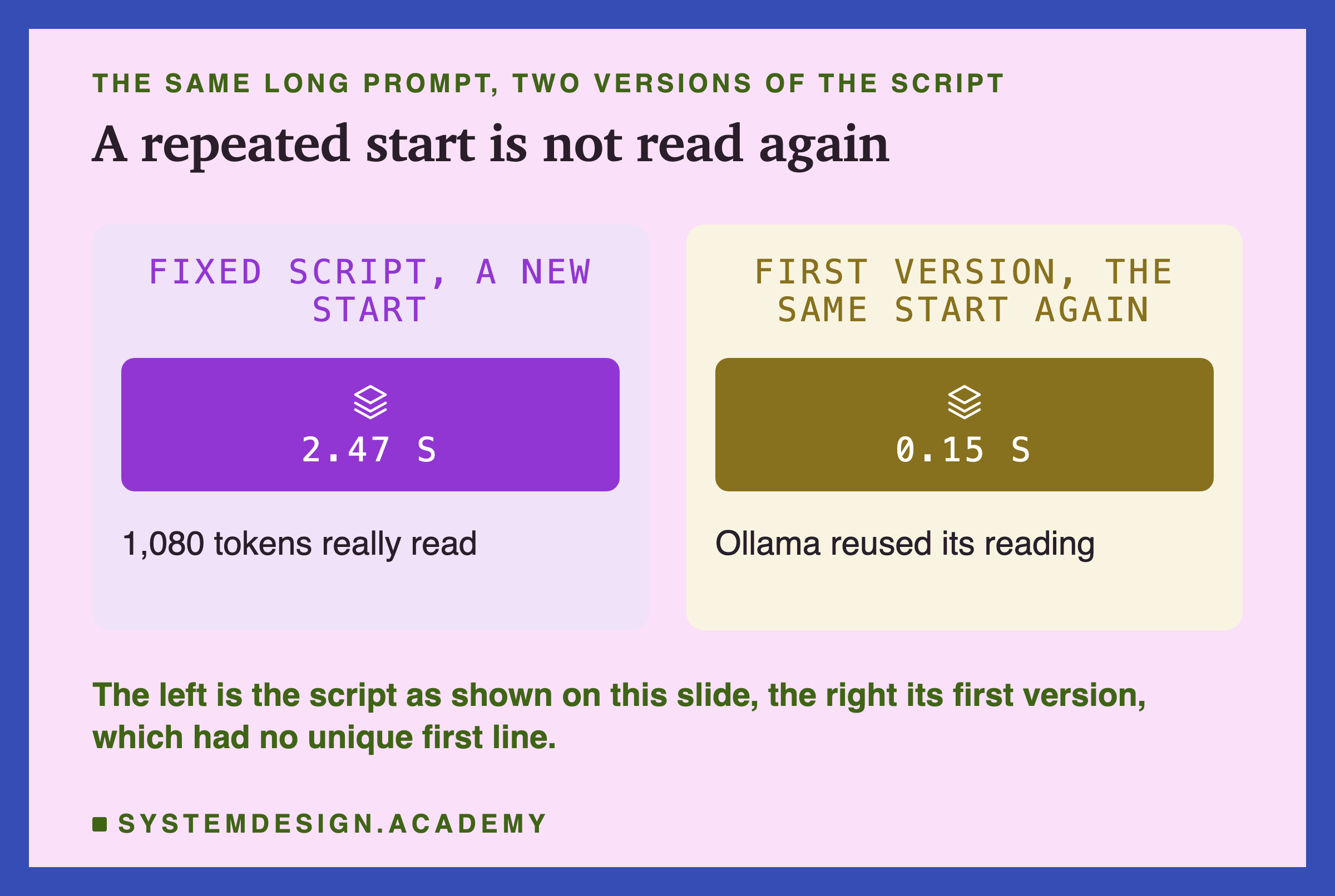
Two panels headed the same long prompt, two versions of the script, titled a repeated start is not read again. The left, fixed script, a new start, shows 2.47 s, 1,080 tokens really read. The right, first version, the same start again, shows 0.15 s, Ollama reused its reading. Beneath: the left is the script as shown on this slide, the right its first version, which had no unique first line.

On the repeat run the long prompt showed its first word after only 0.15 seconds, and it still reported about 1,060 tokens read. Ollama still held the keys and values of that prompt from the earlier run, found the new prompt started the same way, and skipped the reading. The count stays the same; only the time drops. It is the same check as lesson 3: a 1,130-token prompt sent twice took 2.53 seconds to read the first time and 0.04 the second, with the same count both times.

This reuse is useful in real apps, and a later lesson in this chapter looks at it on purpose. For measuring, it is a trap: a timing test that repeats its prompt measures the cache, not the reading. That is why every prompt in this lesson's lab and script starts with its own line.

Does a Long Prompt Slow the Writing?

Once the first word appears, the rest of the reply follows at the writing speed from lesson 3. Does that speed depend on how long the prompt was?

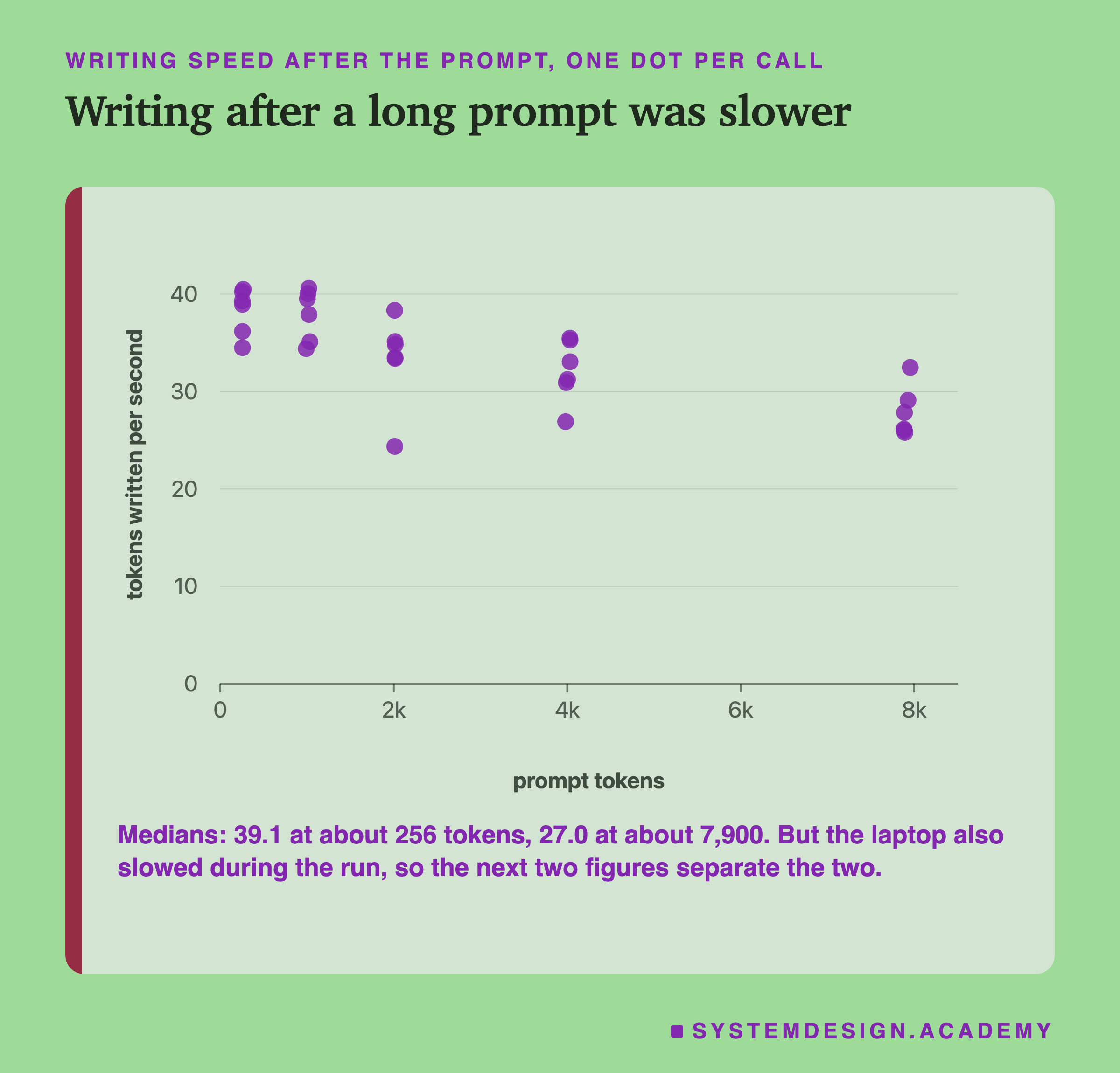
A scatter chart of tokens written per second against prompt tokens, one dot per call. The dots sit between about 34 and 41 at about 256 and 1,000 tokens and between about 26 and 33 at about 7,900. Beneath: medians, 39.1 at about 256 tokens and 27.0 at about 7,900, but the laptop also slowed during the run, so the next two figures separate the two.

At first sight, yes: the median writing speed was 39.1 tokens a second after a 256-token prompt and 27.0 after a 7,900-token prompt. But lesson 3 taught us to check for drift before believing a difference like that.

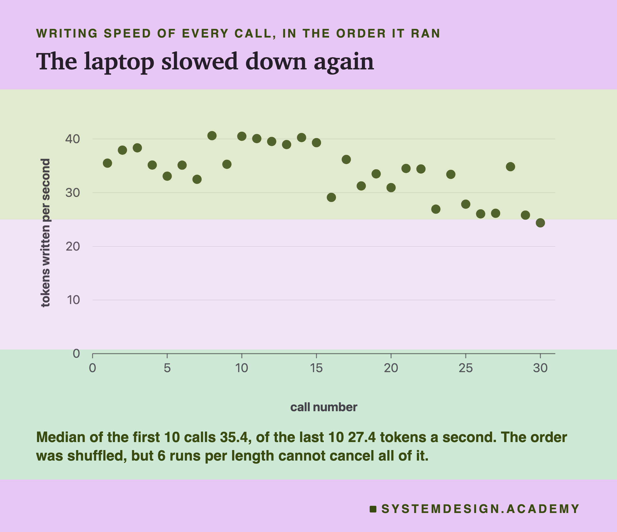
A scatter chart of writing speed of every call in the order it ran, call number along the bottom. The early calls sit between about 33 and 41 tokens per second, and the later calls mostly between about 24 and 35. Beneath: median of the first 10 calls 35.4, of the last 10 27.4 tokens a second, and the order was shuffled, but 6 runs per length cannot cancel all of it.

The laptop slowed again during this run: the median writing speed of the first 10 calls was 35.4 tokens a second, and of the last 10 it was 27.4. The order of the 30 calls was shuffled, so no prompt length was run only at the end. But with only 6 runs per length, the shuffle cannot balance the drift perfectly. Four of the six 7,900-token calls happened to run in the last 10 calls, when the laptop was slow.

Taking the Drift Out, by a Fit

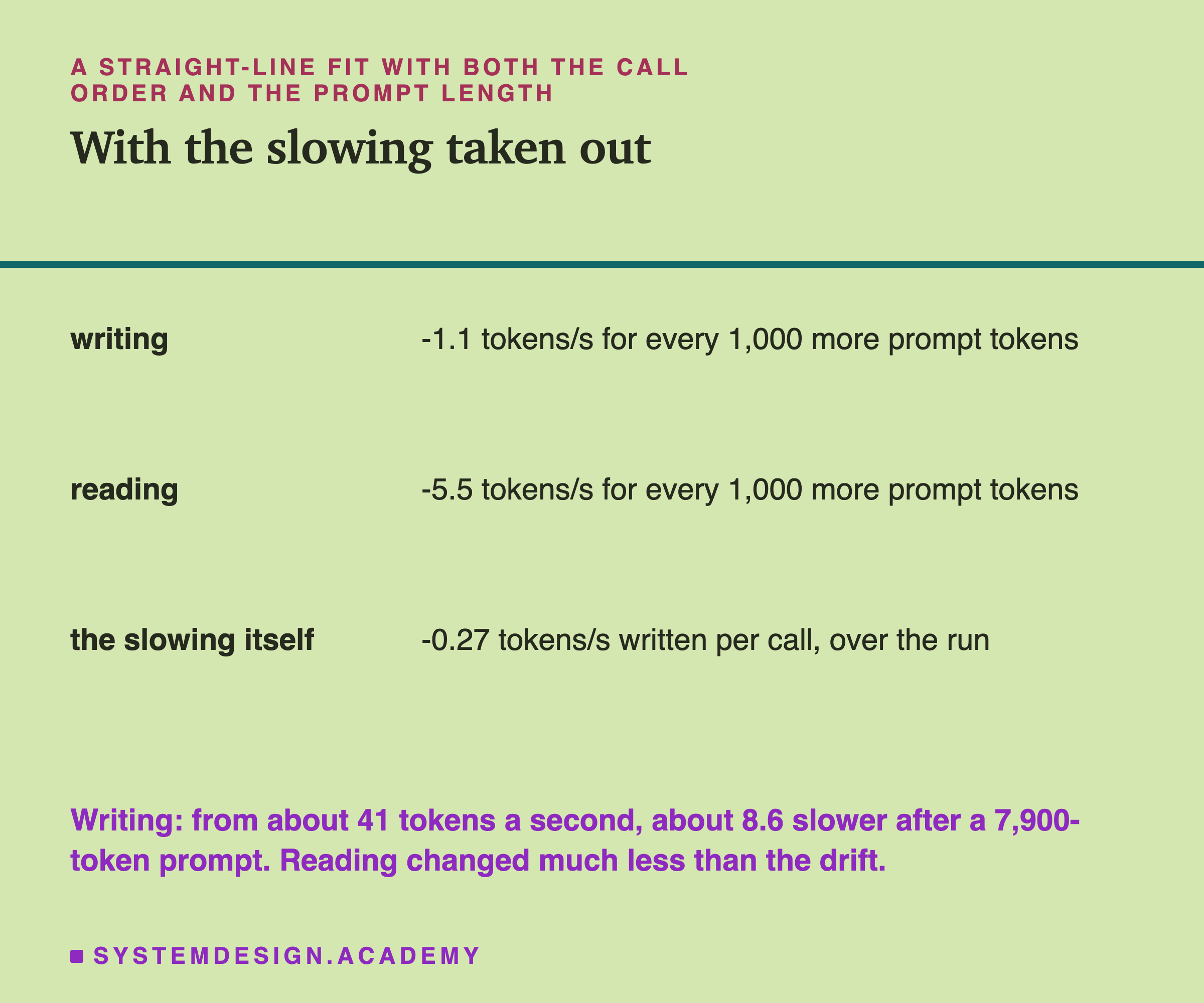
To separate the two effects, I fitted a straight-line model to all 30 calls: writing speed = a starting speed + a change per call number + a change per 1,000 prompt tokens. A fit like this finds the three numbers that make the line pass as close as possible to all the dots. Because call number and prompt length were shuffled, the fit can tell their effects apart.

A table headed a straight-line fit with both the call order and the prompt length, titled with the slowing taken out. Writing: minus 1.1 tokens per second for every 1,000 more prompt tokens. Reading: minus 5.5 tokens per second for every 1,000 more prompt tokens. The slowing itself: minus 0.27 tokens per second written per call, over the run. Beneath: writing, from about 41 tokens a second, about 8.6 slower after a 7,900-token prompt; reading changed much less than the drift.

The fit says writing got about 1.1 tokens a second slower for every 1,000 more prompt tokens, from a starting speed of about 41. For a 7,900-token prompt that is about 1.08 × 7.9 ≈ 8.6 tokens a second slower (1.08 is the fit's slope before rounding), roughly a fifth. So yes, a long prompt does slow the writing, but much less than the raw medians suggested; part of that difference was the laptop, not the prompt.

The same fit for reading speed gave about 5.5 tokens a second slower per 1,000 prompt tokens, against speeds of 190 to 450. Across the whole range of prompt lengths that puts reading about 40 tokens a second slower, around a tenth, while the drift over the 30 calls took about 200 off. So most of the extra wait came from having more to read, and a smaller part from each token getting a little harder to read. That smaller part is why the wait grew about 37 times while the prompt grew about 31 times.

A fit is only as good as its assumptions. It assumes both effects are straight lines and add together. With 30 calls, treat the numbers as sizes to remember, not exact values.

Why Writing Slows Down After a Long Prompt

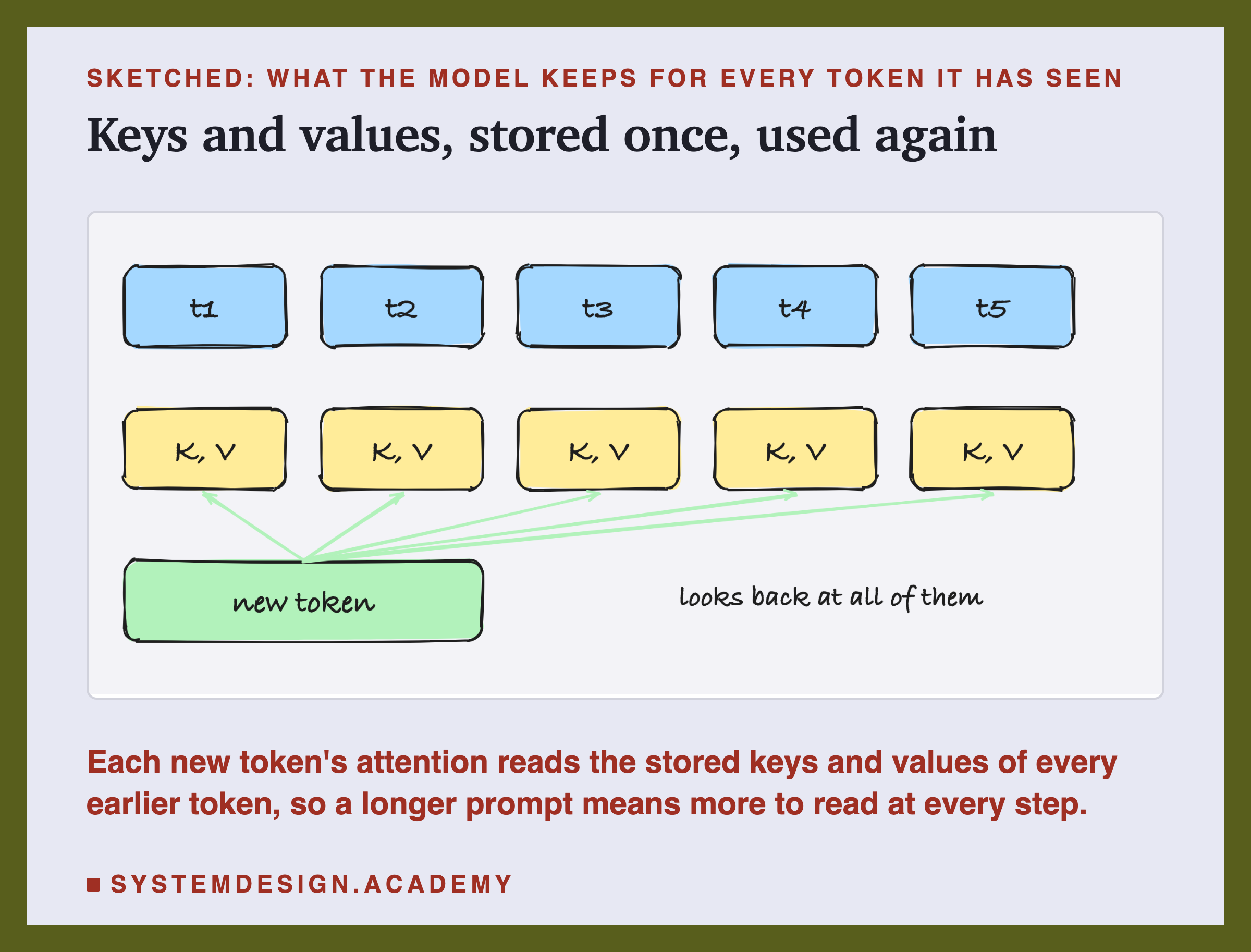
A hand-drawn sketch of five blue token boxes, t1 to t5, each with a yellow box labelled K, V underneath, and a green box labelled new token with an arrow to each of the five stored K, V boxes, marked looks back at all of them. Beneath: each new token's attention reads the stored keys and values of every earlier token, so a longer prompt means more to read at every step.

Lesson 4 showed that every new token looks back, in every layer, at the keys and values of every earlier token. When the model writes, those keys and values are already stored in the , so it does not recompute them. But it still has to read them. After a 256-token prompt, each new token looks back at about 256 stored tokens. After a 7,900-token prompt, it looks back at about 7,900.

That extra looking-back is small compared with the rest of the work each written token does, which is why writing slowed by only about a fifth, not by 31 times. This explanation is general knowledge about how these models run; the lab measured the slowdown, not its cause.

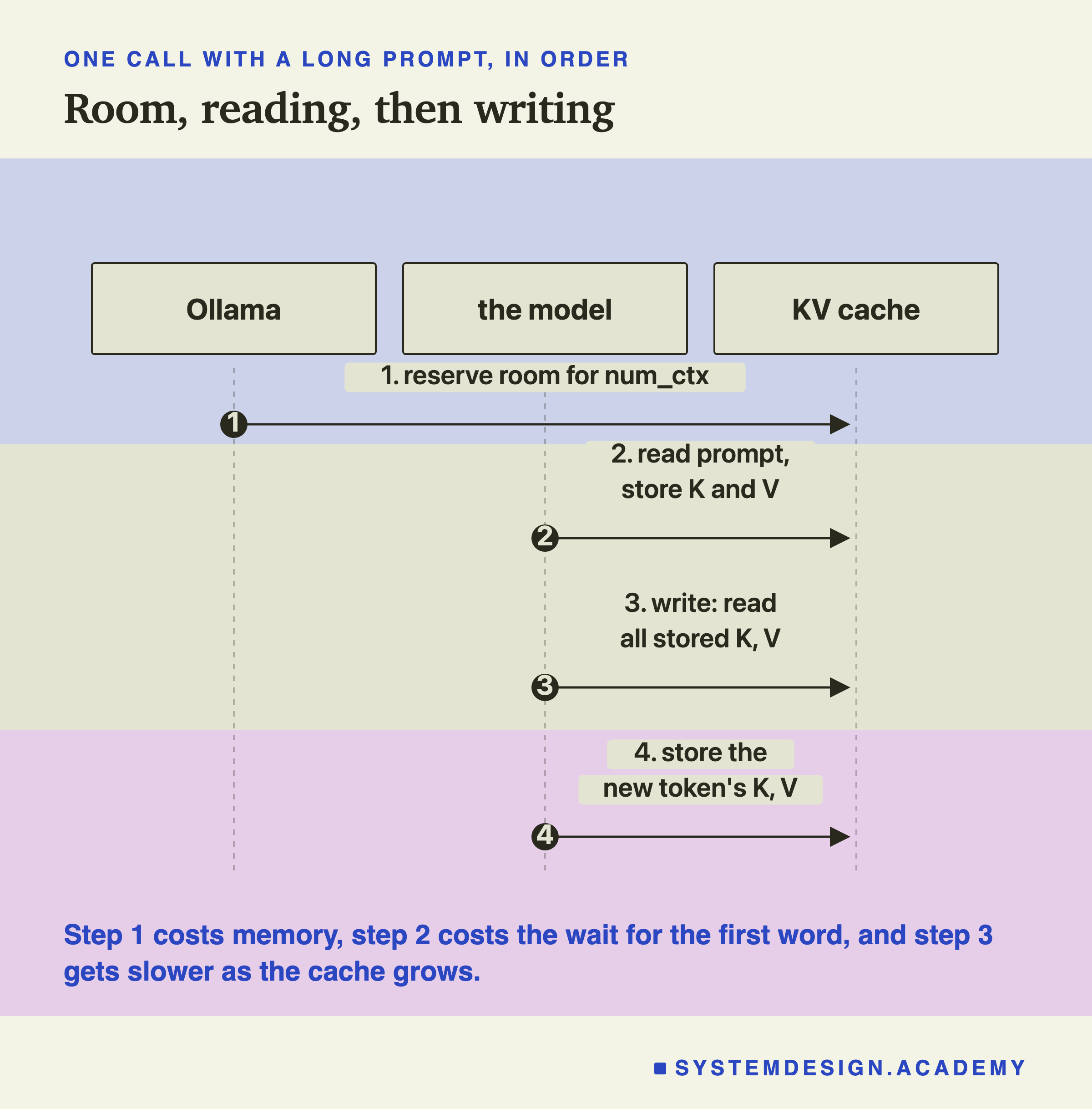
A sequence diagram with three columns: Ollama, the model and the KV cache. Step one, Ollama reserves room for num_ctx. Step two, the model reads the prompt and stores K and V. Step three, the model writes and reads all the stored K and V. Step four, the model stores the new token's K and V. Beneath: step 1 costs memory, step 2 costs the wait for the first word, and step 3 gets slower as the cache grows.

The sequence puts the three costs in order. Reserving room costs memory. Reading costs the wait. Writing with a large cache costs a little speed on every token.

How Big Is One Token's Memory? By Hand

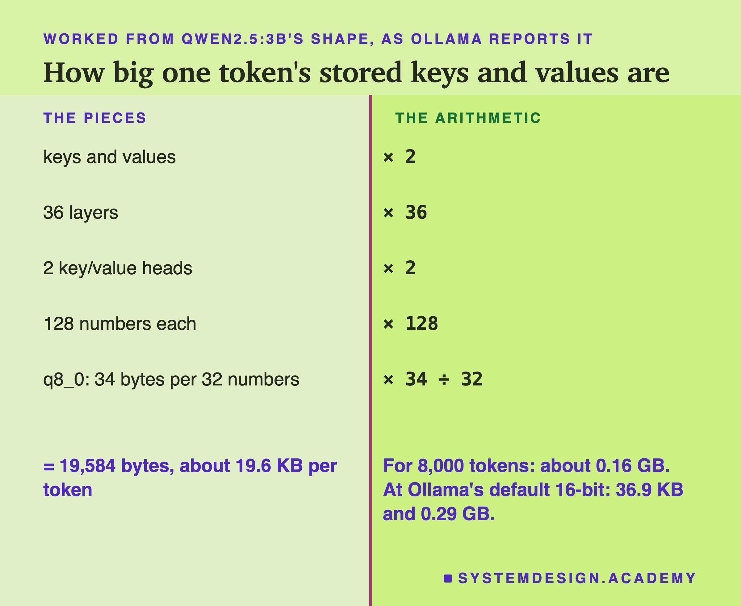
You can work out how much memory the needs from the model's shape. Ollama reports qwen2.5:3b's shape through its /api/show endpoint: 36 layers, 16 attention heads, 2 key/value heads, and 2,048 numbers per word.

A page in two columns titled how big one token's stored keys and values are. Under the pieces: keys and values; 36 layers; 2 key/value heads; 128 numbers each; q8_0, 34 bytes per 32 numbers. Under the arithmetic: times 2, times 36, times 2, times 128, times 34 divided by 32. Beneath, left: equals 19,584 bytes, about 19.6 KB per token. Right: for 8,000 tokens, about 0.16 GB, and at Ollama's default 16-bit, 36.9 KB and 0.29 GB.

Step 1, numbers per head. 2,048 numbers per word divided among 16 heads is 2,048 ÷ 16 = 128 numbers per head.

Step 2, numbers per token. For one token, the model stores a key and a value (× 2), in every one of 36 layers (× 36), for each of the 2 key/value heads (× 2), each 128 numbers long (× 128). So 2 × 36 × 2 × 128 = 18,432 numbers.

Step 3, bytes per token. This depends on how each number is stored, and here I nearly got it wrong. Ollama's default stores each number as a 16-bit number, 2 bytes, which would make 18,432 × 2 = 36,864 bytes, about 36.9 KB. I first worked the lesson out that way. Then the memory measurement on the next slide came out lower than that arithmetic, so I looked at how the running server was started. On this laptop Ollama was installed with Homebrew, and Homebrew's service file sets OLLAMA_KV_CACHE_TYPE to q8_0. In q8_0, each number is stored in 8 bits, 1 byte, in groups of 32 that share one 2-byte scale, so 32 numbers take 34 bytes. That gives 18,432 × 34 ÷ 32 = 19,584 bytes, about 19.6 KB per token, a little over half.

Step 4, per prompt. For 8,000 tokens: 8,000 × 19,584 ≈ 157 million bytes, about 0.16 GB. With Ollama's default 16-bit storage it would be about 0.29 GB.

So check your own server before you use either number: the lab records the storage format it found, and the command line of Ollama's llama-server process shows it after --cache-type-k. Storing the numbers in 8 bits loses a little precision in exchange for half the memory; this lesson did not measure whether that changed any answers. Lesson 4's model shared each key/value set between several query heads; this model does the same, 16 query heads sharing 2 key/value heads, and that sharing is exactly what keeps the number this small.

Memory for the Window, Measured

Now compare the arithmetic with what Ollama reports. The lab loaded the model with five window sizes and read the size Ollama reports for the loaded model from its /api/ps endpoint.

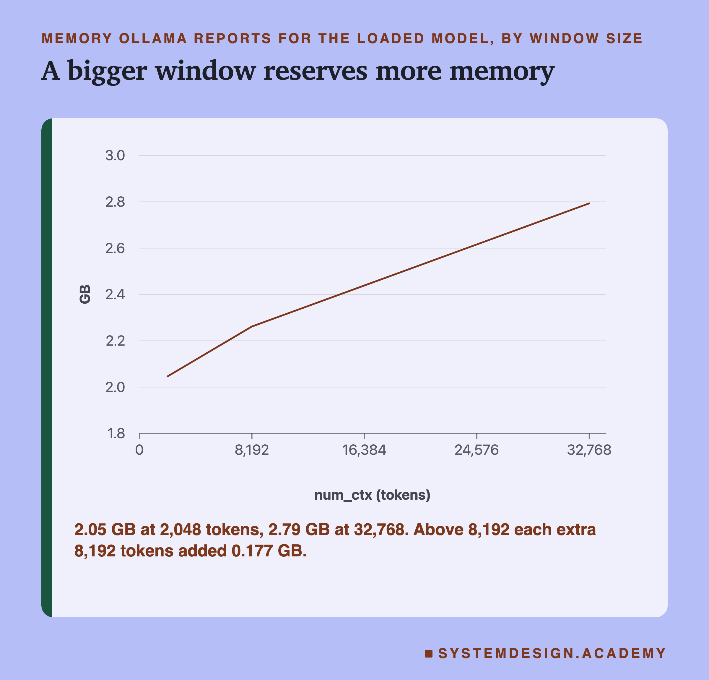
A line chart of memory Ollama reports for the loaded model, by window size, num_ctx from 0 to 32,768 along the bottom and gigabytes from 1.8 to 3.0 up the side. The line rises from 2.05 GB at 2,048 tokens through 2.26 at 8,192 to 2.79 GB at 32,768, steeper in the first step and straight after that. Beneath: 2.05 GB at 2,048 tokens, 2.79 GB at 32,768, and above 8,192 each extra 8,192 tokens added 0.177 GB.

The reported size was 2.046 GB with a window of 2,048 tokens, 2.262 GB at 8,192, 2.439 at 16,384, 2.616 at 24,576 and 2.793 at 32,768. Notice that the prompt was only one word each time. The memory depends on the window you ask for, not on the prompt you send, because Ollama reserves the room when it loads the model.

Check it against the arithmetic. From 8,192 upwards, each extra 8,192 tokens added exactly 0.177 GB, which is 0.177 GB ÷ 8,192 ≈ 21.6 KB per token. The q8_0 arithmetic says 19.6 KB, so the keys and values explain about nine tenths of each step; the other 2 KB or so per token is some other buffer that also grows with the window, which this lab did not break down. The 16-bit arithmetic, 36.9 KB, is far above what was measured, which is how the storage format was caught.

The first step is different: from 2,048 to 8,192 the window grew by 6,144 tokens and the size by 0.215 GB, about 35.0 KB per token, more than the later steps. I cannot explain that from this lab. The reported size is Ollama's own estimate for the model and its buffers, not a measurement of the whole process, and it may include parts sized in steps rather than per token.

What holds either way: a bigger window reserves more memory, whether or not you fill it. Going from 2,048 to 32,768 tokens added about 0.75 GB to a model that is about 2 GB, more than a third.

The Lab Report

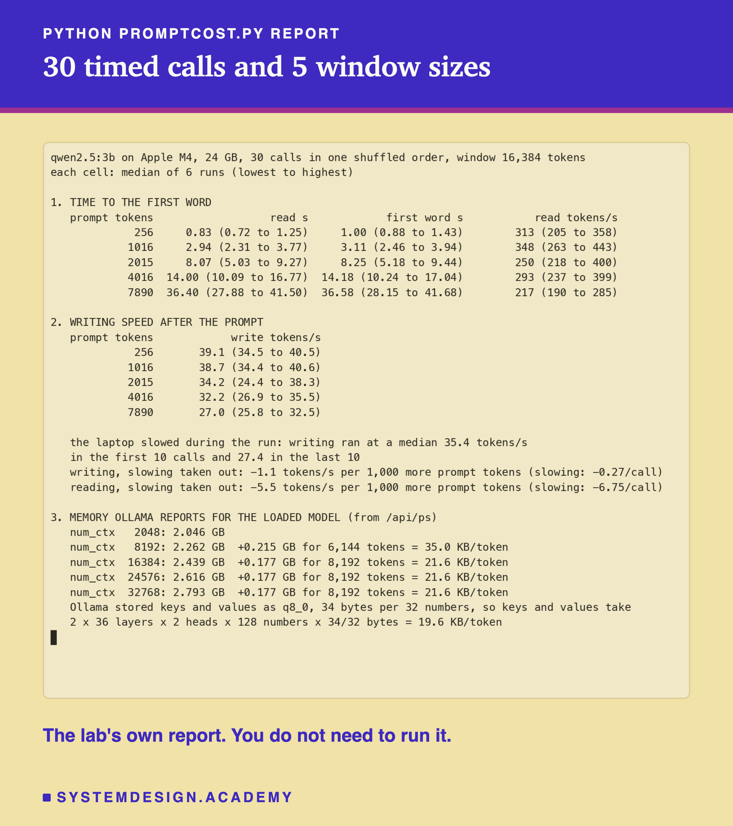
A real terminal recording of python promptcost.py report on qwen2.5:3b, Apple M4, 24 GB, 30 calls in one shuffled order, window 16,384 tokens. Section 1, time to the first word: for about 256, 1,016, 2,015, 4,016 and 7,890 prompt tokens, the median read time with its range, the median first-word time, 1.00, 3.11, 8.25, 14.18 and 36.58 seconds, and reading speed. Section 2, writing speed after the prompt: medians 39.1, 38.7, 34.2, 32.2 and 27.0 tokens per second; the laptop slowed from 35.4 in the first 10 calls to 27.4 in the last 10; writing, slowing taken out, minus 1.1 tokens per second per 1,000 prompt tokens; reading, minus 5.5. Section 3, memory Ollama reports: 2.046, 2.262, 2.439, 2.616 and 2.793 GB for windows of 2,048 to 32,768, with the KB per token for each step, and the line that Ollama stored keys and values as q8_0, 34 bytes per 32 numbers, so 19.6 KB per token.

The lab, scripts/labs/generate/promptcost.py, made 30 timed calls with prompts aimed at 256, 1,024, 2,048, 4,096 and 8,192 tokens, which landed at about 256, 1,016, 2,015, 4,016 and 7,890, 6 each, in one shuffled order with a fixed seed. Every call used a window of 16,384 tokens, so only the prompt changed, and every prompt started with its own line. Then it measured the reported memory for five window sizes.

Read section 1 for the wait, section 2 for the writing speed and the drift, and section 3 for the memory. The ranges in brackets are wide, as they were in lesson 3, which is why the lesson leans on medians, the fit, and differences large enough to survive the noise.

The lab also guards against the cache trap. A reused prompt keeps its token count but reads impossibly fast, so the lab fails if any call read faster than 2,000 tokens a second. The fastest real reading was 443.

Putting a Price on 8,000 Tokens

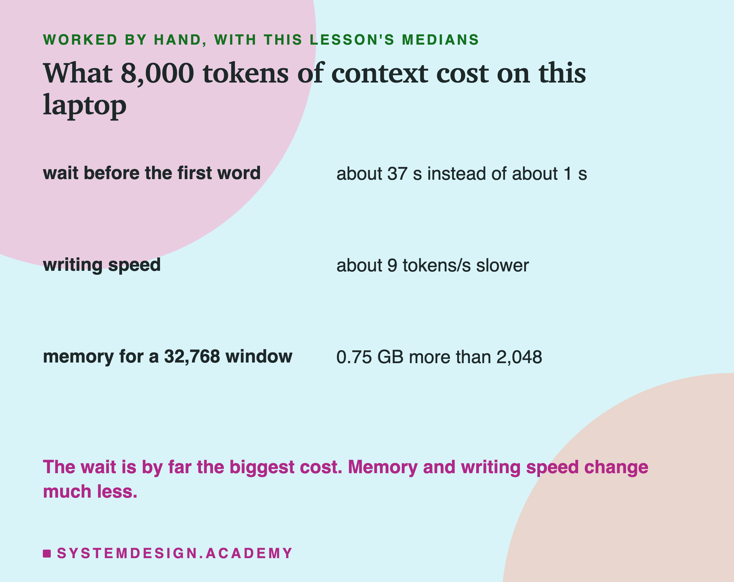
Here are the three costs side by side, for a prompt of about 8,000 tokens on this laptop.

A worked table headed worked by hand, with this lesson's medians, titled what 8,000 tokens of context cost on this laptop. Wait before the first word: about 37 s instead of about 1 s. Writing speed: about 9 tokens per second slower. Memory for a 32,768 window: 0.75 GB more than 2,048. Beneath: the wait is by far the biggest cost, and memory and writing speed change much less.

The wait before the first word went from about 1 second to about 37. The writing, once it started, was about 9 tokens a second slower. And a window big enough to hold long prompts reserved about 0.75 GB more memory than a small one.

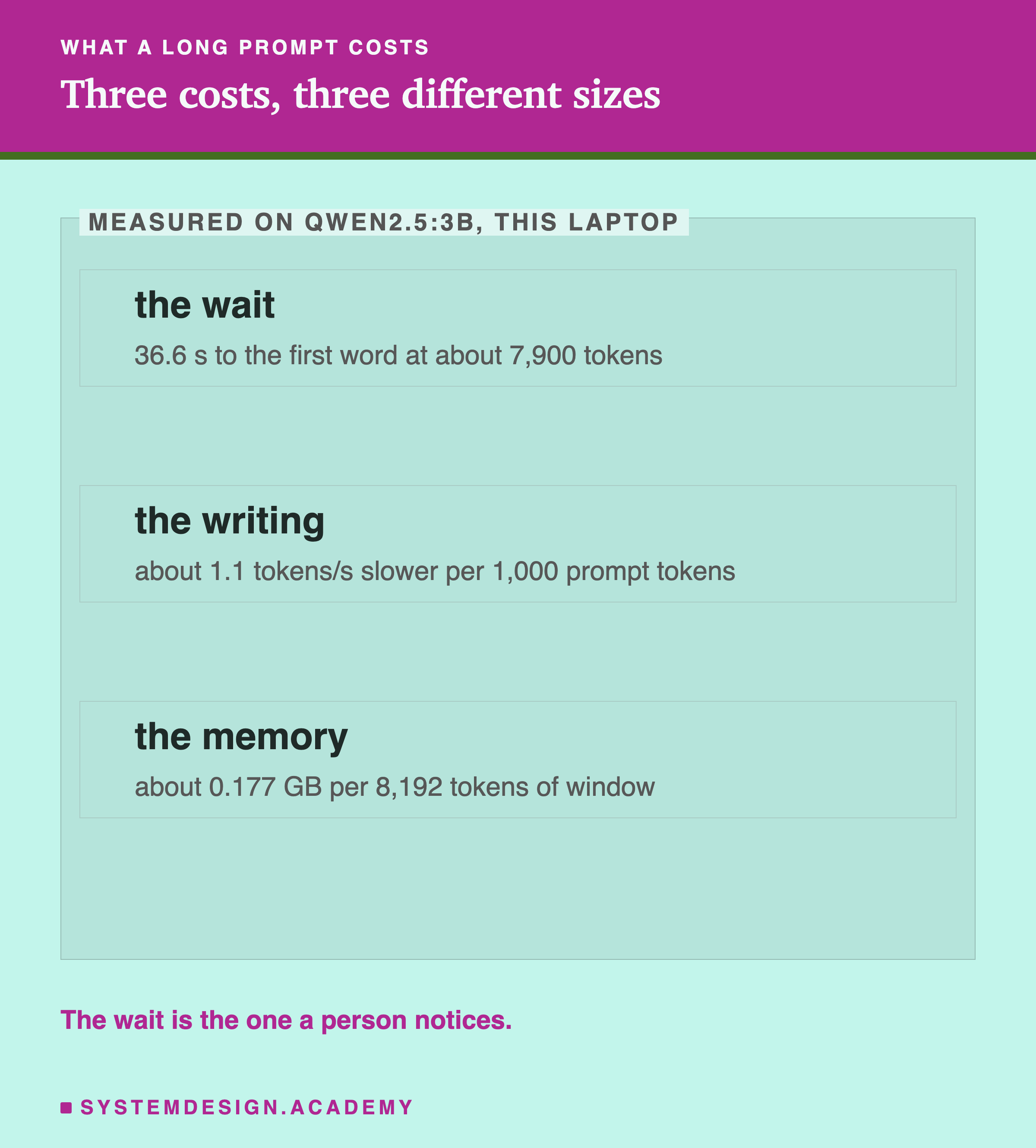
For a person using a chat app, the wait is the cost that matters. Writing a little slower is hardly noticeable, and the memory is a one-time reservation. For a server handling many people at once, memory matters more, because every loaded window takes room that other requests could use.

Three editorial boxes inside a frame labelled measured on qwen2.5:3b, this laptop, titled three costs, three different sizes. The wait: 36.6 s to the first word at about 7,900 tokens. The writing: about 1.1 tokens per second slower per 1,000 prompt tokens. The memory: about 0.177 GB per 8,192 tokens of window. Beneath: the wait is the one a person notices.

When Is a Long Prompt Worth It?

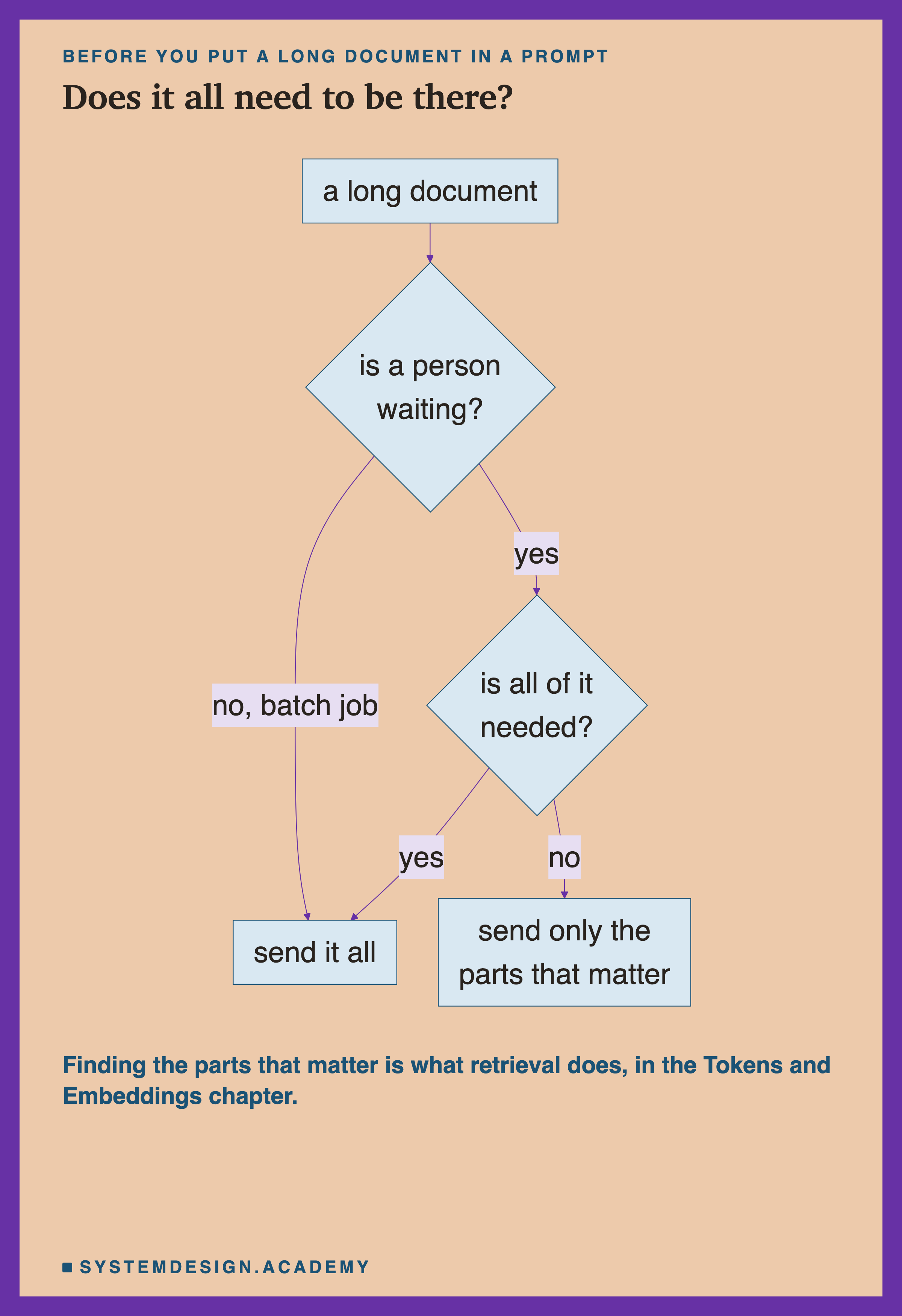
A flowchart. A long document leads to a decision, is a person waiting? No, batch job, leads to send it all. Yes leads to a second decision, is all of it needed? Yes leads to send it all. No leads to send only the parts that matter. Beneath: finding the parts that matter is what retrieval does, in the Tokens and Embeddings chapter.

If nobody is waiting, as in a batch job that summarises documents overnight, a long prompt only costs time you were not watching. Send what the job needs.

If a person is waiting, ask whether the model really needs all of it. Often it needs one section, not the whole document. Picking that section is exactly what the search methods of the Tokens and chapter do: embed the document in pieces, find the pieces closest to the question, and send only those. A 300-token excerpt instead of an 8,000-token document turns a wait of over half a minute into about a second on this laptop.

When you do need a long prompt, stream the reply (lesson 3), so at least the writing is visible as it happens, and tell the person the model is reading.

Estimate the Costs in Your Browser

This box has no model. It holds this lesson's measured medians and the hand arithmetic, and lets you estimate the three costs for any prompt length.

For 3,000 tokens it prints a first word after about 11.2 seconds, writing at about 37.7 tokens a second, and about 0.06 GB of keys and values. The estimate between measured lengths is a straight line, so treat it as a rough guide, and remember these numbers are from one busy laptop.

The Code, Part by Part

Streaming. first_word_time.py sets "stream": True. Ollama then sends one small JSON object per token, one per line, instead of one big answer at the end. The loop for line in resp reads them as they arrive.

The clock. start = time.time() is taken just before sending. The first time a piece has any response text, the script records time.time() - start. That is the wait a person would see. The last piece has "done": true and carries the same timing fields as lesson 3, including load_duration.

The unique line. f"Request {time.time()}.\n" puts the current time at the start of every prompt, so no two runs share a start and Ollama cannot reuse its reading.

The lab. promptcost.py builds the 30 prompts from this course's lesson text, shuffles their order with random.Random(11), and calls Ollama in raw mode with num_ctx 16,384. Its report computes the medians and ranges, the first-10 and last-10 comparison, and the straight-line fit with numpy's least-squares solver. Its memory part unloads the model, loads it with each window size, and reads the reported size from /api/ps. The figures recompute the same fit from the saved calls, so they cannot disagree with the report.

Common Mistakes

Timing a repeated prompt. Ollama reuses a start it has already read. The count stays the same and the time collapses. Give each timed prompt its own start.

Blaming the prompt for all of a slowdown. In this run, part of the slower writing after long prompts was the laptop slowing down. Shuffle the order and check for drift before you name a cause.

Setting the biggest window "just in case". The window is reserved when the model loads, whether or not you use it. Going from 2,048 to 32,768 tokens added about 0.75 GB here.

Sending a whole document when a person is waiting. A wait of over half a minute before the first word feels broken. Send the parts that matter.

Trusting one run. The first-word time at about 7,900 tokens ranged from 28.2 to 41.7 seconds over six runs.

Reading a reported memory figure as the whole story. Ollama's reported size is its own estimate for the model and its buffers. For the real memory of the process, use your operating system's tools.

What This Lab Can and Cannot Tell You

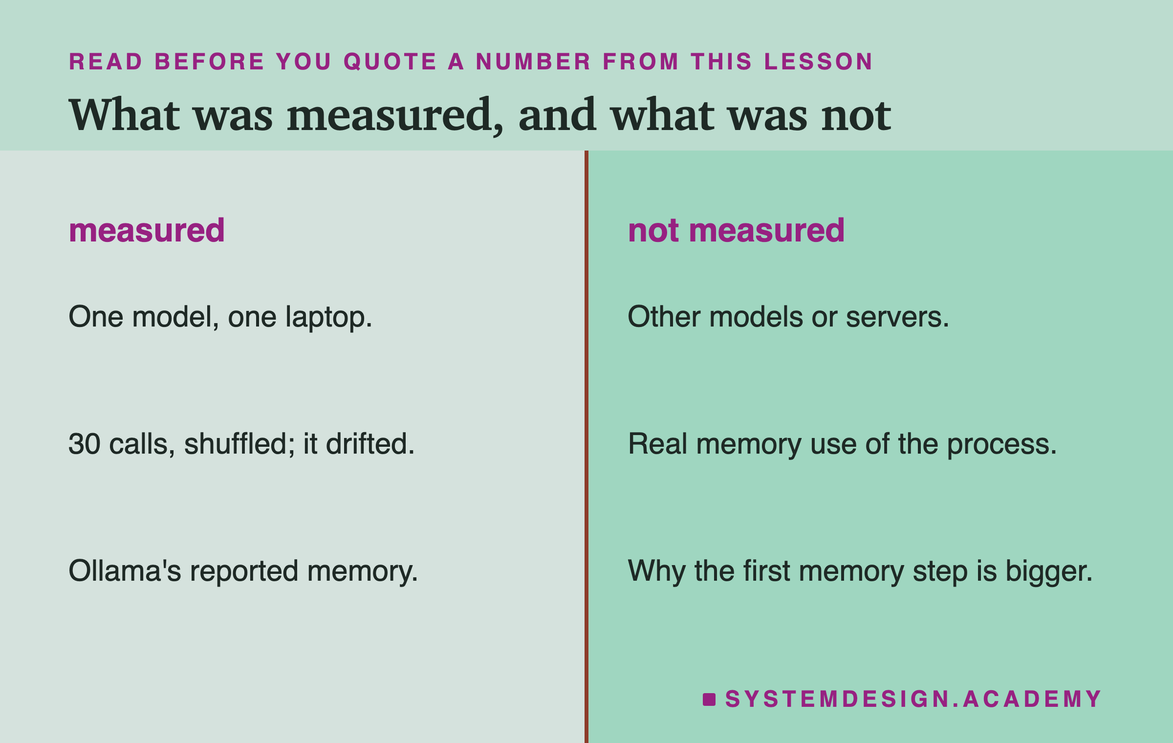
A page in two columns. Under measured: one model, one laptop; 30 calls, shuffled, it drifted; Ollama's reported memory. Under not measured: other models or servers; real memory use of the process; why the first memory step is bigger.

The lab measured one model on one laptop, with 30 timed calls that drifted, and it read Ollama's reported memory rather than measuring the process. Other models, graphics cards and servers will give different numbers; the shape, a wait that grows with the prompt and memory that grows with the window, is what to expect.

It did not explain why the reported memory grew by 35.0 KB per token in the first step and 21.6 after that, or what the 2 KB per token above the q8_0 arithmetic is. It did not measure the real memory used by the process, and it did not test whether q8_0 storage changed any answers.

Two brand cards. Ollama: qwen2.5:3b, Apple M4, 24 GB. Python: 30 timed calls, 5 window sizes.

Everything ran locally with Ollama and Python, so you can repeat it on your own machine.

What to Do on Monday

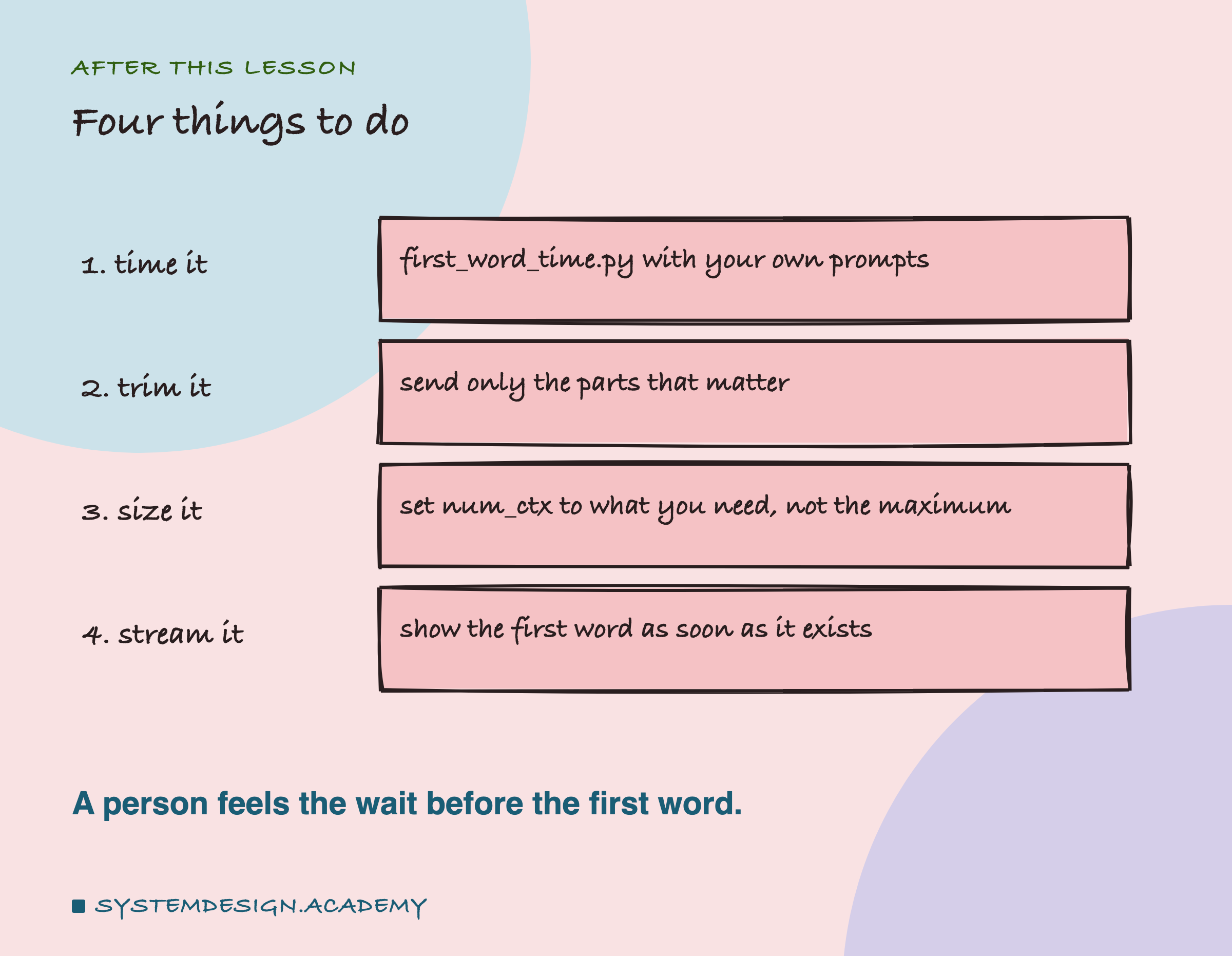
A hand-drawn list of four steps. 1, time it: first_word_time.py with your own prompts. 2, trim it: send only the parts that matter. 3, size it: set num_ctx to what you need, not the maximum. 4, stream it: show the first word as soon as it exists. Beneath: a person feels the wait before the first word.

Run first_word_time.py with a prompt like the ones your app really sends, and write down the time to the first word. If it is more than a couple of seconds and a person is waiting, look at what you send and cut what the answer does not need. Then set num_ctx to fit your longest real prompt plus its reply, not to the largest number the model allows.

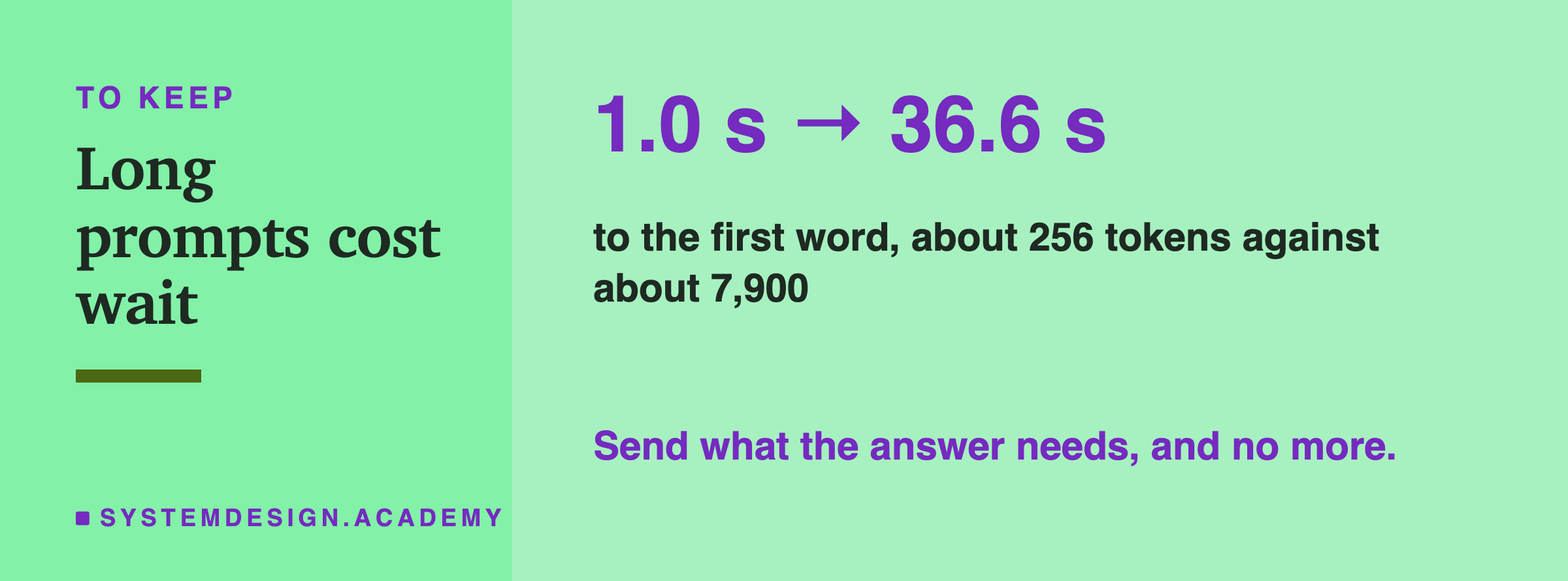
A closing card. In large type: 1.0 s to 36.6 s. Beneath: to the first word, about 256 tokens against about 7,900. In the accent colour: send what the answer needs, and no more.

A later lesson in this chapter uses the on purpose: when many requests share the same start, such as the same system prompt, the model can skip reading it again, and the wait for those requests drops sharply.

Knowledge Check

Knowledge Check

4 questions - Score 80% to pass

Q1

On this laptop, which cost of a 7,900-token prompt would a person in a chat app notice most?

Q2

A 1,130-token prompt is sent twice in a row. Ollama reports 1,130 tokens read both times, but the reading takes 2.53 seconds, then 0.04. Why?

Q3

qwen2.5:3b stores keys and values for 36 layers and 2 key/value heads of 128 numbers. With Ollama's default of 2 bytes per number, about how much memory do 10,000 tokens of keys and values need?

Q4

Writing was 39.1 tokens/s after short prompts and 27.0 after long ones, but the laptop was also slowing down during the run. What did the lesson do before blaming the prompt length?