Let me start with a teacher and her mark book.

Last term, she took one point off for every careless slip. This term, the school changed the rule: careless slips no longer cost anything. Nothing else changed. Same students, same kind of tests, same mark book. And in that book, both terms' marks sit in one column, called "mark".

Now think about what can go wrong. A head teacher compares this term's marks with last term's and says the class improved. Did it? Partly, maybe. But part of the rise is only the new rule. A scholarship committee ranks students using marks from both terms together. A student who did well last term is now compared with students marked by a kinder rule.

The teacher could fix this in a few ways. She could re-mark every old paper with the new rule. That is a lot of work. She could re-mark only the last few weeks. She could write "old rule" and "new rule" next to each mark, so at least everyone can see the difference. Or she could do nothing and hope it does not matter.

Machine learning has exactly this problem. In this lesson I measure each of those choices on real data.

This lesson uses the same shop, customers and question as the rest of the chapter. If any of that is new, please read what a feature is first. That lesson built six features from each customer's history: recency, frequency, money, return share, tenure and products. The question is always the same. At the start of a month, will this customer buy something in the next 30 days?

Two definitions from that lesson matter here. Money was net spend: every line added up, and since the shop records a return as a negative amount, returns are taken away. Frequency was the number of separate purchase invoices.

In the lesson on online and offline consistency, one serving choice was to read "money" as purchases only and leave returns out. That lesson measured what happened when only the serving side did this. Here I go further. I treat it as a deliberate change of definition, and ask what happens when you retrain, backfill half the history, or keep the old name.

Two other lessons are close to this one, and I do not repeat them. Data versioning is about keeping the exact raw data that trained a model. Data contracts is about a producer changing the shape or meaning of the records it sends. This lesson is about something narrower: one feature's definition changing, while the raw data stays exactly the same.

Please read this slide slowly if any word is new. Every slide after it uses these words.

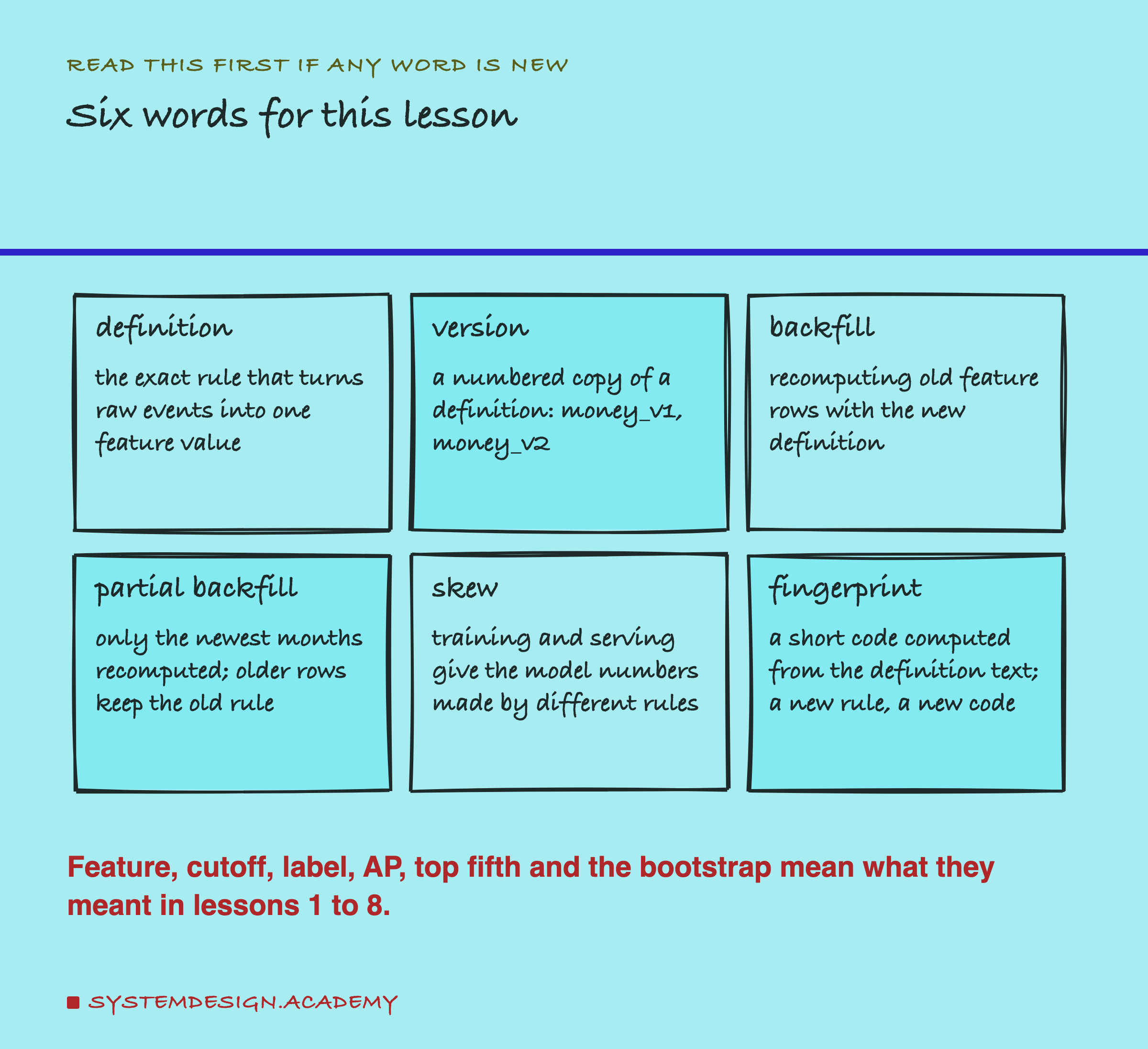
A feature's definition is the exact rule that turns raw events into one number. "Add up every line before the cutoff" is one definition of money. "Add up the purchase lines only" is another. They use the same raw data and give different numbers.

A version is a numbered copy of a definition. I call the old rule v1 and the new rule v2, and when I want the name to carry the version, I write money_v1 and money_v2.

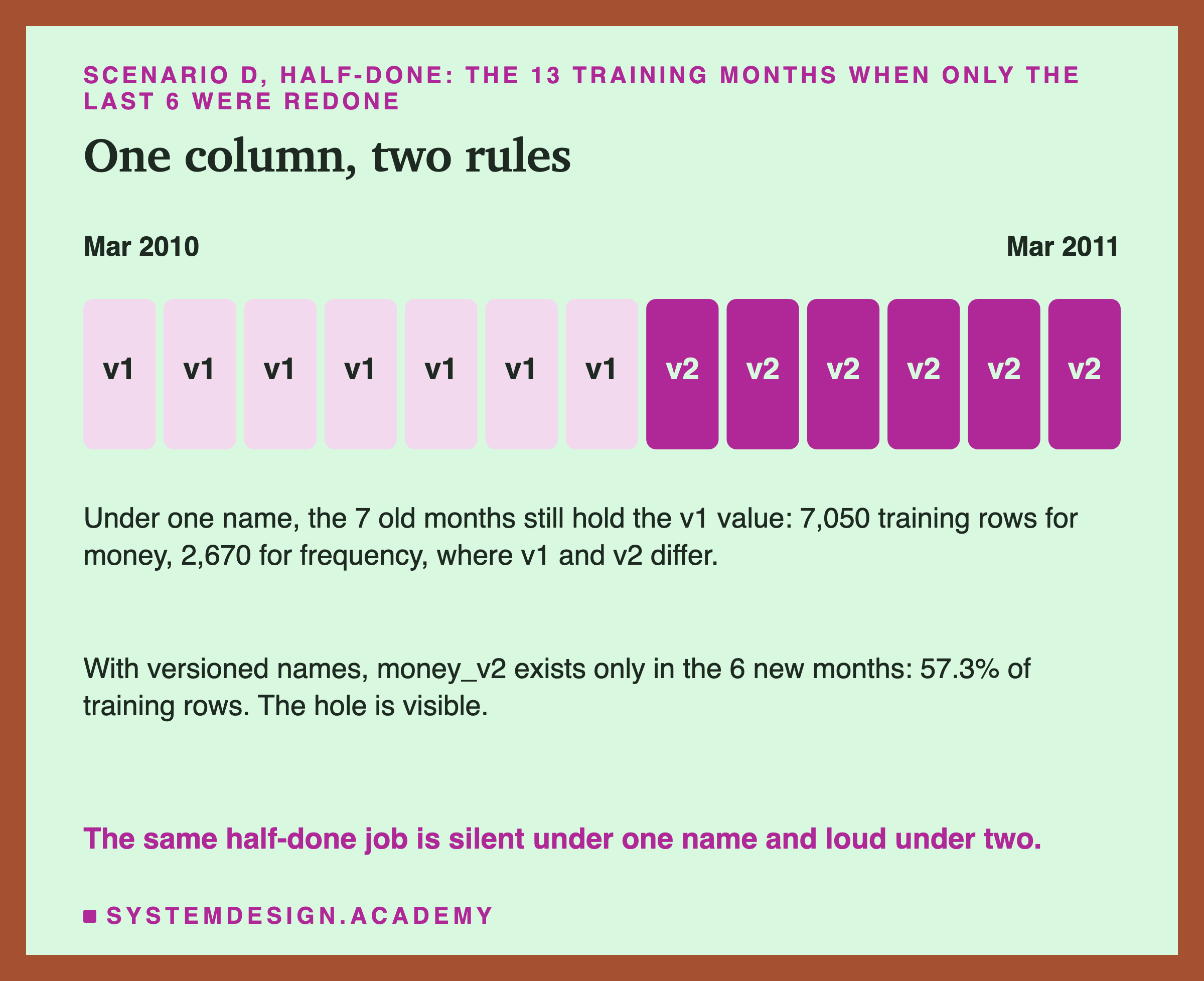
A backfill recomputes the old feature rows with the new definition, so that the whole history follows one rule. In the classroom, that is re-marking every old paper. A partial backfill recomputes only the newest rows. The older rows keep the old rule, usually under the same name.

Skew, short for train/serve skew, means the model was trained on numbers made by one rule, and is given numbers made by another rule when it is used. A fingerprint is a short code computed from the text of a definition. Change one word of the rule, and the code changes.

Feature, cutoff, label, average precision (AP), seed, top fifth and bootstrap mean what they meant in lessons 1 to 8. I explain the bootstrap again where it matters.

Here is one real customer, number 12346, with everything they did before 1 July 2011. Lesson 5 showed the same customer.

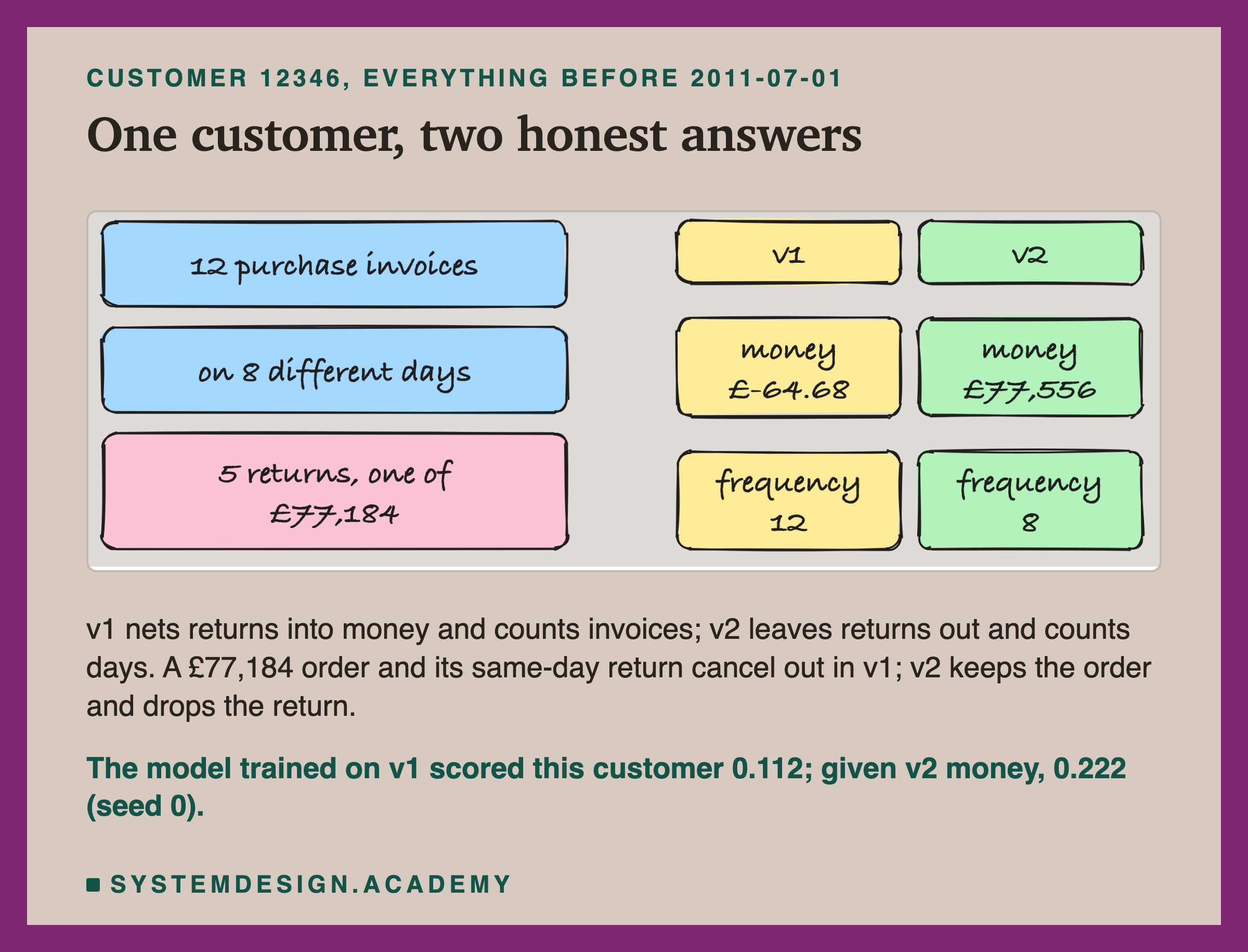
This customer placed 12 purchase invoices, but only on 8 different days. On some days they placed two or three separate orders. They also made 5 returns. One return was huge: on 18 January 2011 they ordered goods worth £77,183.60 and returned the whole order the same day.

Under v1, that order and its return cancel out, and their money is minus £64.68. Under v2, returns are left out, so the big order counts and the return does not. Their money becomes £77,556.46. Frequency moves too: 12 invoices under v1, 8 days under v2.

Which number is right? Both are. Net spend and gross spend are both fair ideas of "money". Invoices and days are both fair ideas of "how often". A team can have a good reason to switch. Maybe the finance team reports gross sales and wants the features to match. Maybe two invoices on one day are really one shopping trip.

The problem is not which rule is better. The problem is what happens to a model and to old data when the rule changes. At seed 0, the model trained on v1 gave this customer a score of 0.112. Given the v2 money, the same model gave 0.222, almost double, without any error or warning.

When a team changes a definition, the change can reach the model in several ways. I measured five.

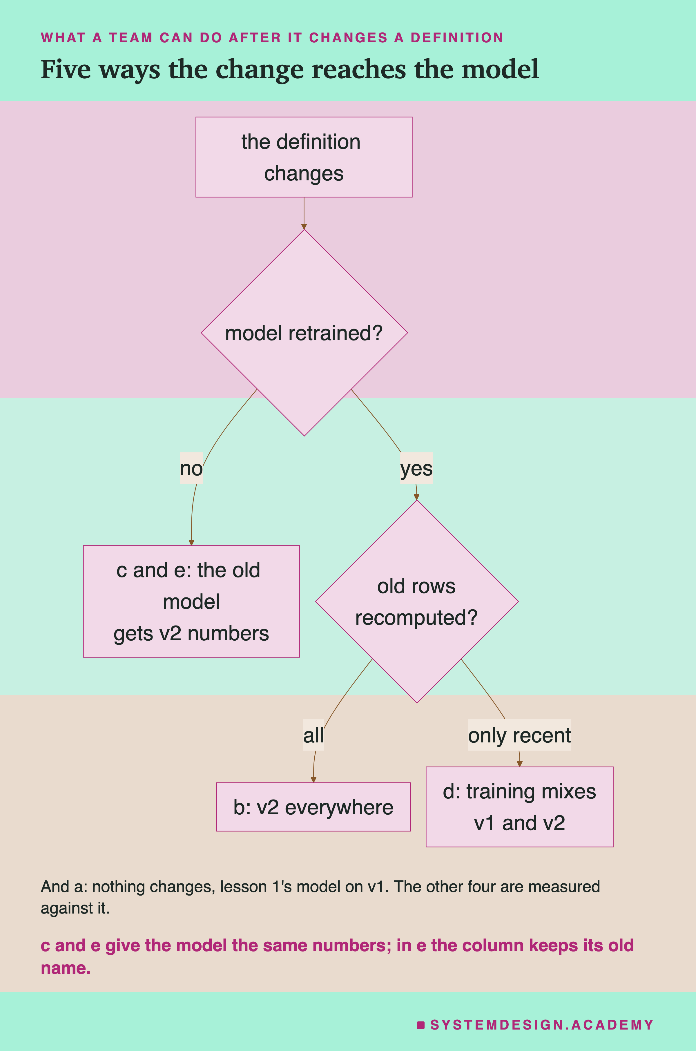
a. Nothing changes. Train on v1, serve v1. This is exactly lesson 1's model, and every other scenario is measured against it.

b. The change done fully. Backfill every training month with v2, retrain, and serve v2.

c. The serving code was updated to v2, but the model was not retrained. In this scenario the names carry the version, so the model expects money_v1 and receives money_v2.

e. The same as c, except the column is still called money on both sides. I call this the silent case. The model receives exactly the same numbers in c and e, so their scores are equal by construction. The lab checks this, and I never use it as evidence. The two differ only in what a check can see.

d. A partial backfill. The team recomputed only the last 1, 3, 6 or 9 of the 13 training months with v2. The older months still hold v1, under the same column. The model is retrained on that mix and served v2. This is very common in practice: backfills are slow and expensive, and they often stop part way.

I measured each scenario for both changes: money and frequency.

Before measuring, I checked what three feature stores say about a changed definition, in their own documentation. A feature store is a system that computes, stores and serves feature values. I recorded every quote in results/ver-factcheck.json.

Feast is an open-source feature store, and the last lesson of this chapter uses it. Its documentation marks feature view versioning as alpha and experimental. It says that "Versions are created only when Feast detects an actual change to the feature view definition (schema or UDF)". A UDF, user-defined function, is code you write to compute a feature. It also says: "Each version requires its own materialization." Materialization means computing the values and writing them into the store. So a new version starts empty until you fill it. Its known limits include that joining features "from different versions of the same feature view in get_historical_features is not supported".

Hopsworks, another feature store, gives each feature group a version number. If you do not give one, its docs say, "the APIs will create a new version by default with a version number equals to the highest existing version number plus one."

Tecton, a commercial feature platform, says: "Changes to a Feature View's transformation or entities are therefore considered destructive and will result in the rematerialization of feature values." So Tecton recomputes the values itself.

I have not run any of these three in this lesson. This is what their documentation says, checked on 1 October 2026. In my own lab, the features live in a pandas table, and a pandas column is only a name. Nothing in records which rule made it.

Here is the silent case, e, as a live service would see it.

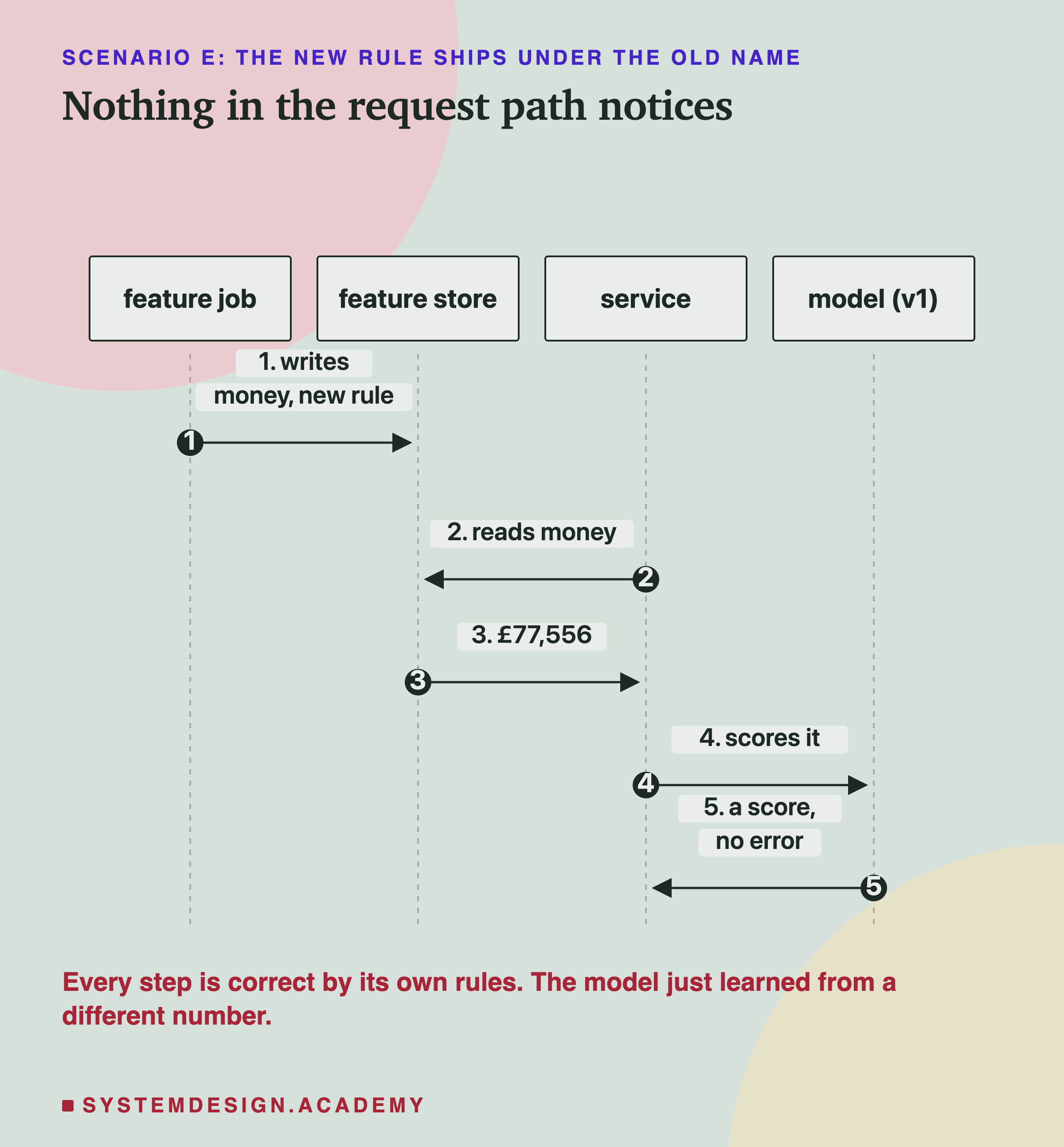
The nightly feature job was updated, so it writes money with the new rule. The service asks for money, as it always has. The store answers with £77,556.46 for customer 12346. The model scores it and returns a number.

No step failed. The job did what its new code says. The store kept a value of the right type. The service asked for a column that exists. The model received a number in a range it has seen before. Every part is correct by its own rules, and yet the model was trained on a different meaning of that column.

A check that looks only at types and names cannot see this. To catch it, something must know the rule itself. Later slides measure which checks did.

I wrote the lab's design into the docstring of scripts/labs/features/feature_versioning.py before it first ran. Before writing it, I knew one result already: lesson 5 had measured that serving purchases-only money to the v1 model lowered test AP by about 0.00049. That is scenario c for money here, so I expected to reproduce it. I had not counted how many rows the frequency change touches, and I had not trained any model on a v2 column.

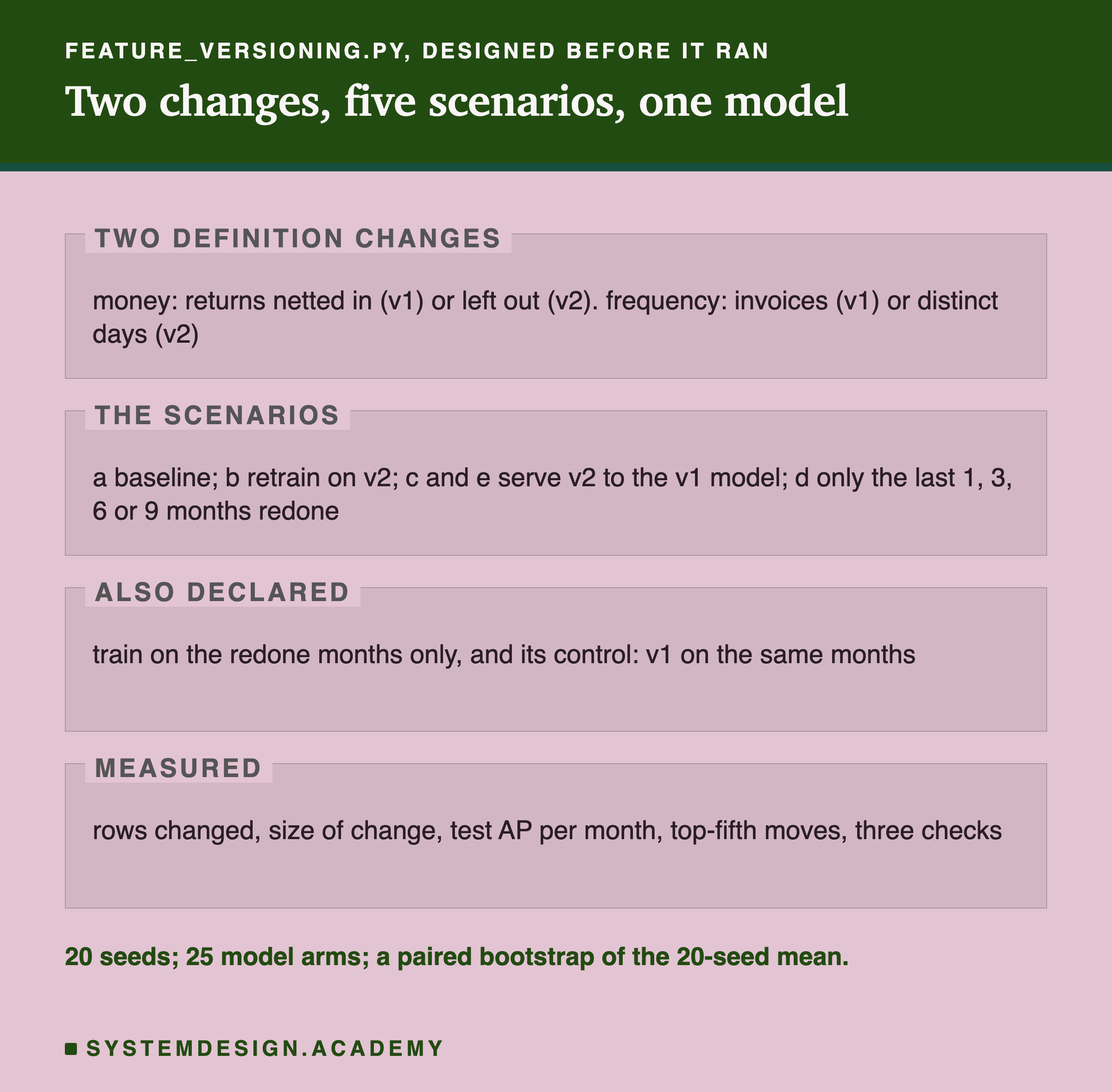
The task and the model are the chapter's own. Train on 13 monthly cutoffs from March 2010 to March 2011, and test on 5 cutoffs from July to November 2011. The model is scikit-learn's HistGradientBoostingClassifier with its default settings. The six features come from lesson 1's own code, imported, not copied. I built the two v2 columns from the same raw lines, using only events before each cutoff.

One more choice for a half-done backfill. Besides mixing v1 and v2 (scenario d), a team could train only on the months that were redone, and throw the older months away. I call this "drop". It also trains on fewer rows and fewer seasons, so I added a control: train on v1, on the same few months. A control is a second arm that differs in only one way, so the difference between them shows the effect of that one thing. Here, drop minus control shows the effect of v2 at equal data.

Three checks. A name check compares the column names the model was trained on with the names the service sends. A compares a code computed from each column's definition text. A compares the numbers themselves, explained on its own slide. The first two give their answer , once the names or texts differ, so I report them as what a guard would see, not as findings. The drift check is the only one that is measured.

This is a real recording of the report script, ver_report.py, in its full mode, on the laptop where the lab ran. It refits every model the lab trained, reruns the bootstrap and checks every number.

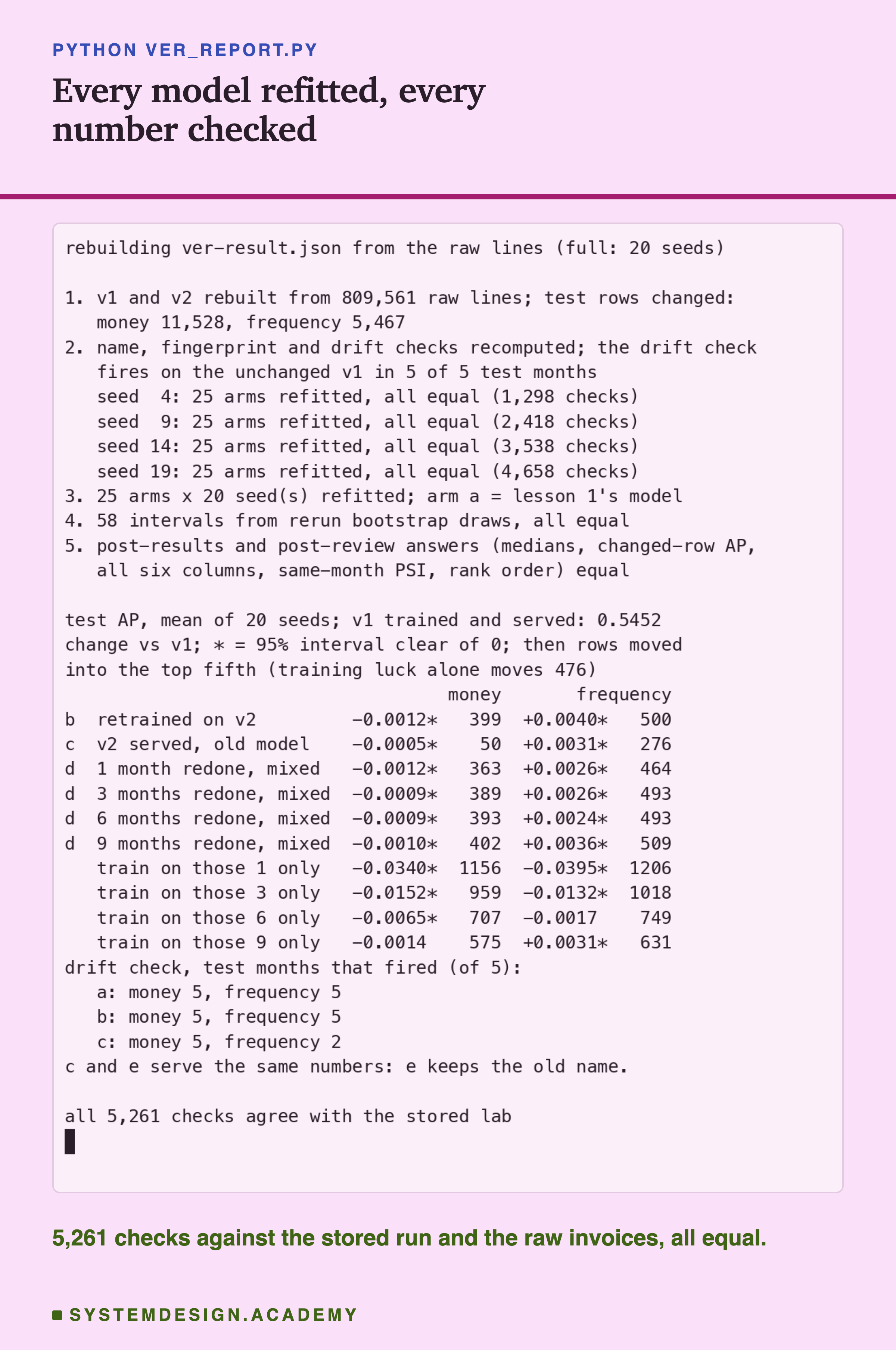
The report does not reuse the lab's code for the parts that matter. It rebuilds all eight columns from the raw invoice lines with its own grouping code: the six v1 features and the two v2 ones. They must match. It counts changed rows, measures the size of each change and computes the drift check with its own code. Then it refits every model with the same seeds, and requires every stored AP, top-fifth count and score change to come back.

It also checks that scenario a equals lesson 1's model on all 20 seeds. It has a fast mode, python ver_report.py fast, which refits only seed 0 of every arm and recomputes the intervals from the stored bootstrap draws. If anything disagrees, it stops with an error.

Before any model, the plain counts.

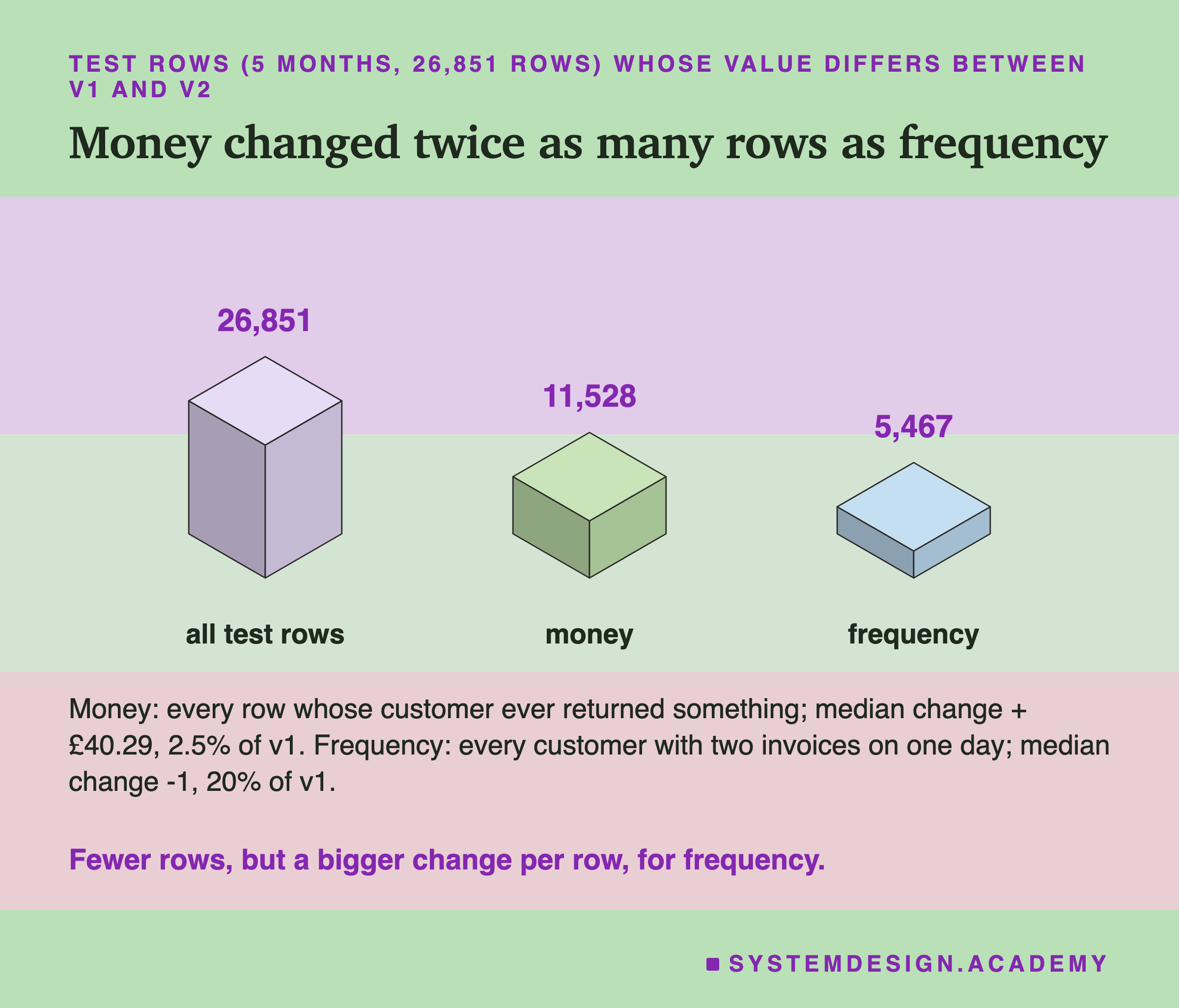
The money change touched 11,528 of the 26,851 test rows. That is exactly the rows whose customer had made at least one return before the cutoff, and the lab checks that count. For most of them the change was small: the median rise was £40.29, about 2.5 percent of their v1 money. For a few it was enormous, like customer 12346.

The frequency change touched 5,467 test rows: exactly the customers who had at least two purchase invoices on the same day. The median change was -1, but relative to a small count that is big: a median of 20 percent of the v1 value. The largest drop was 132.

In the training months, money changed 17,515 of 44,521 rows and frequency 7,507.

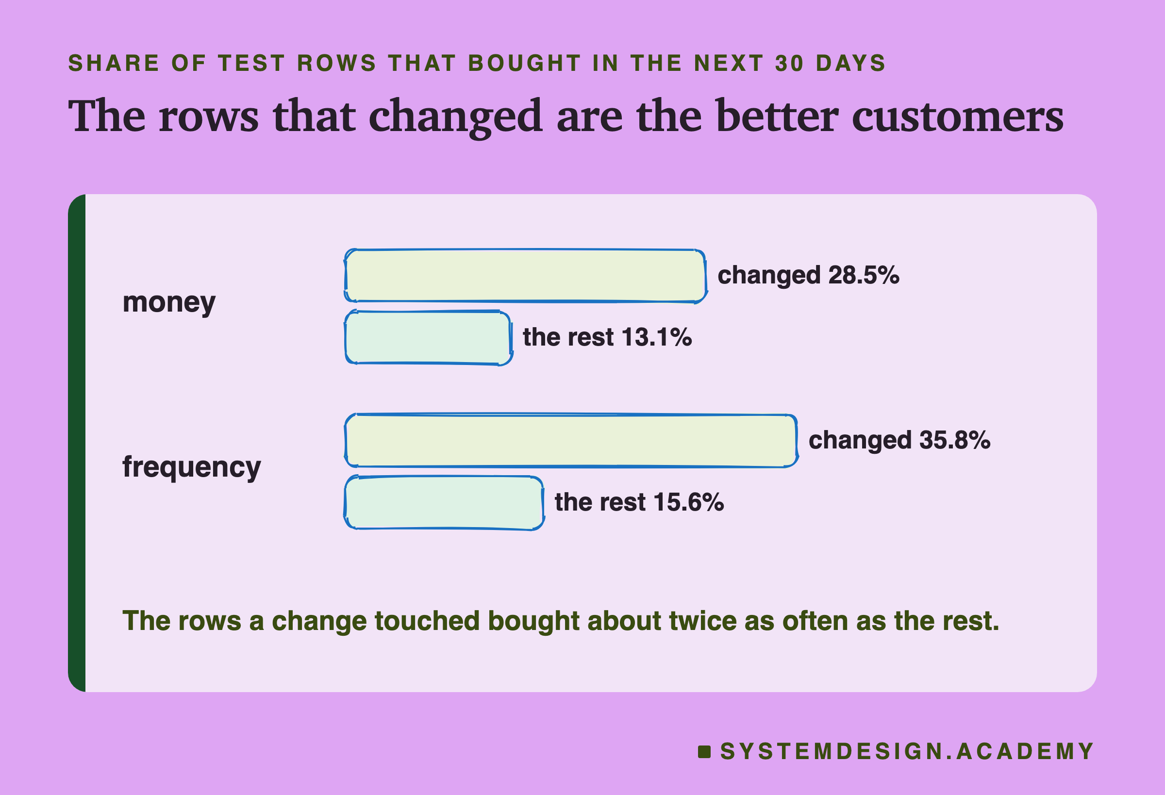
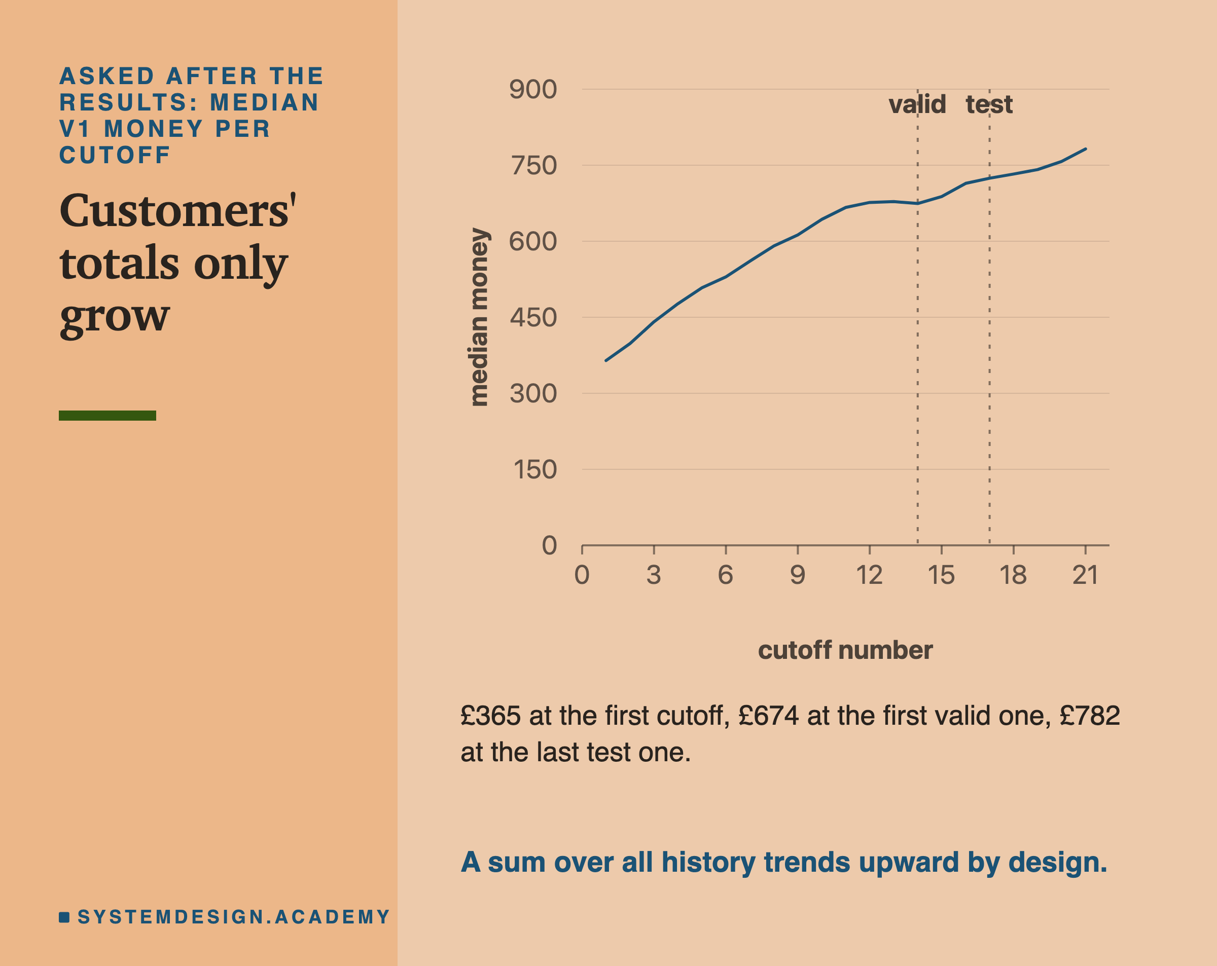
Here is why the touched rows matter more than their count suggests. Customers who make returns, and customers who order twice in a day, are active customers. Among the rows money changed, 28.5 percent bought in the next 30 days, against 13.1 percent of the rest. Among the rows frequency changed, 35.8 percent bought, against 15.6 percent. A definition change does not land on random rows. It lands on the busy customers, who are exactly the ones a model tries to rank near the top.

Here is the main result. The v1 model, trained and served on v1, scored a mean test AP of 0.5452 over 20 seeds.

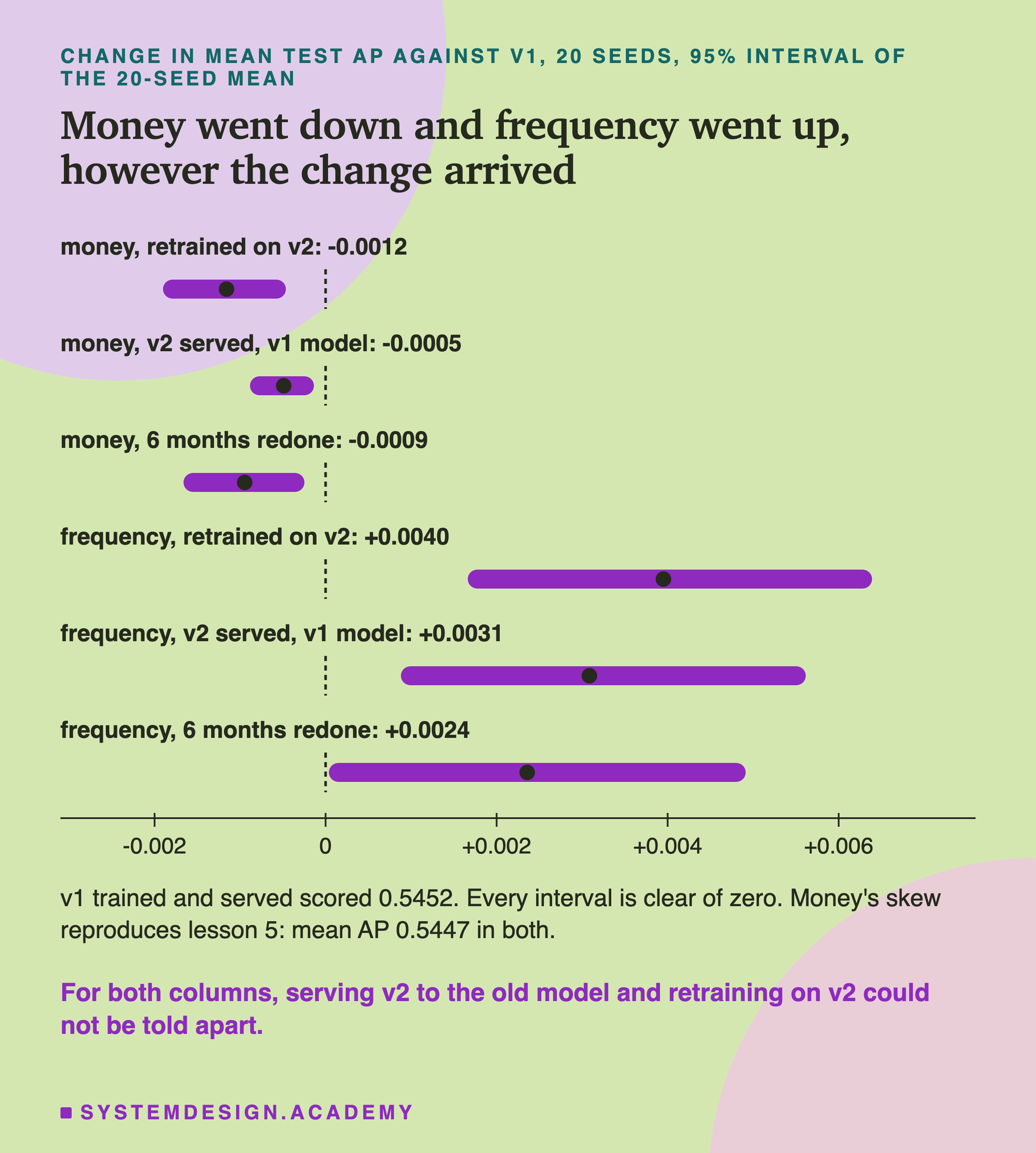
On this shop's test months, money v2 was a slightly worse feature, and frequency v2 a slightly better one. Retrained on v2 with a full backfill, scenario b, money lowered test AP by 0.0012, with an interval from -0.0019 to -0.0005. Frequency raised it by 0.0040, from +0.0017 to +0.0064. Those are small changes, but measurable.

The silent skew moved the score the same way, a little less. Serving v2 to the v1 model, scenario c and also e, lowered AP by 0.0005 for money, interval -0.0009 to -0.0001, in all 20 of 20 seeds. That matches lesson 5's measurement of the same change: mean AP 0.5447 in both. The largest gap between a seed here and the same seed there was 0.000006. The tiny gap comes from lesson 5 adding money in a loop, which rounds the last digits differently.

For frequency, the skew raised AP by 0.0031, from +0.0009 to +0.0056, again in 20 of 20 seeds. I did not expect that at all.

For both columns, the skew and the full retrain could not be told apart. For money, c minus b ran from about 0 to +0.0013; for frequency, from -0.0027 to +0.0009. So in this lab, forgetting to retrain cost about the same as retraining. That is not a reason to skip retraining. One likely reason is that both changes kept the order of most values, and a tree model mostly cares about order.

A rank correlation measures how well two lists keep the same order; 1 means exactly the same order. A reviewer asked for it after the results, so the lab labels it as a reviewer check. Within each test month, v1 and v2 had a rank correlation of 0.986 to 0.987 for money and 0.988 to 0.990 for frequency. A later slide comes back to this.

I measured two kinds of luck, as in every lesson of this chapter.

Luck in training. With more than 10,000 training rows, this model turns on early stopping by itself and keeps 10 percent of the training rows aside, chosen at random. The seed moves that choice. So every number is a mean over 20 runs with seeds 0 to 19. The models trained on only one month have 4,607 rows, below 10,000, so for them the seed changes nothing. The lab records that for every fit.

Luck in which customers were tested. A bootstrap draws the test customers again at random, within each month, with repeats allowed, and recomputes the score. I did it 1,000 times. In each draw I recomputed the AP of every arm for all 20 seeds and averaged them, so one interval covers both kinds of luck. The same draw is used for every arm, which is what paired means.

The middle 95 percent of the 1,000 differences is the 95% interval. I call a difference measurable only when its interval sits entirely on one side of zero. Otherwise I say it cannot be told apart from zero. I also count, seed by seed, how often an arm beat scenario a. For money skew it was below in 20 of 20 seeds; for money retrained, below in 14 of 20.

The bootstrap code is lesson 8's, imported. Before trusting its fast way of computing AP, it checks it against scikit-learn's average_precision_score on 78 cases.

AP is an average over thousands of customers. A shop that contacts the top fifth of each month sees something more direct: which people are on the list.

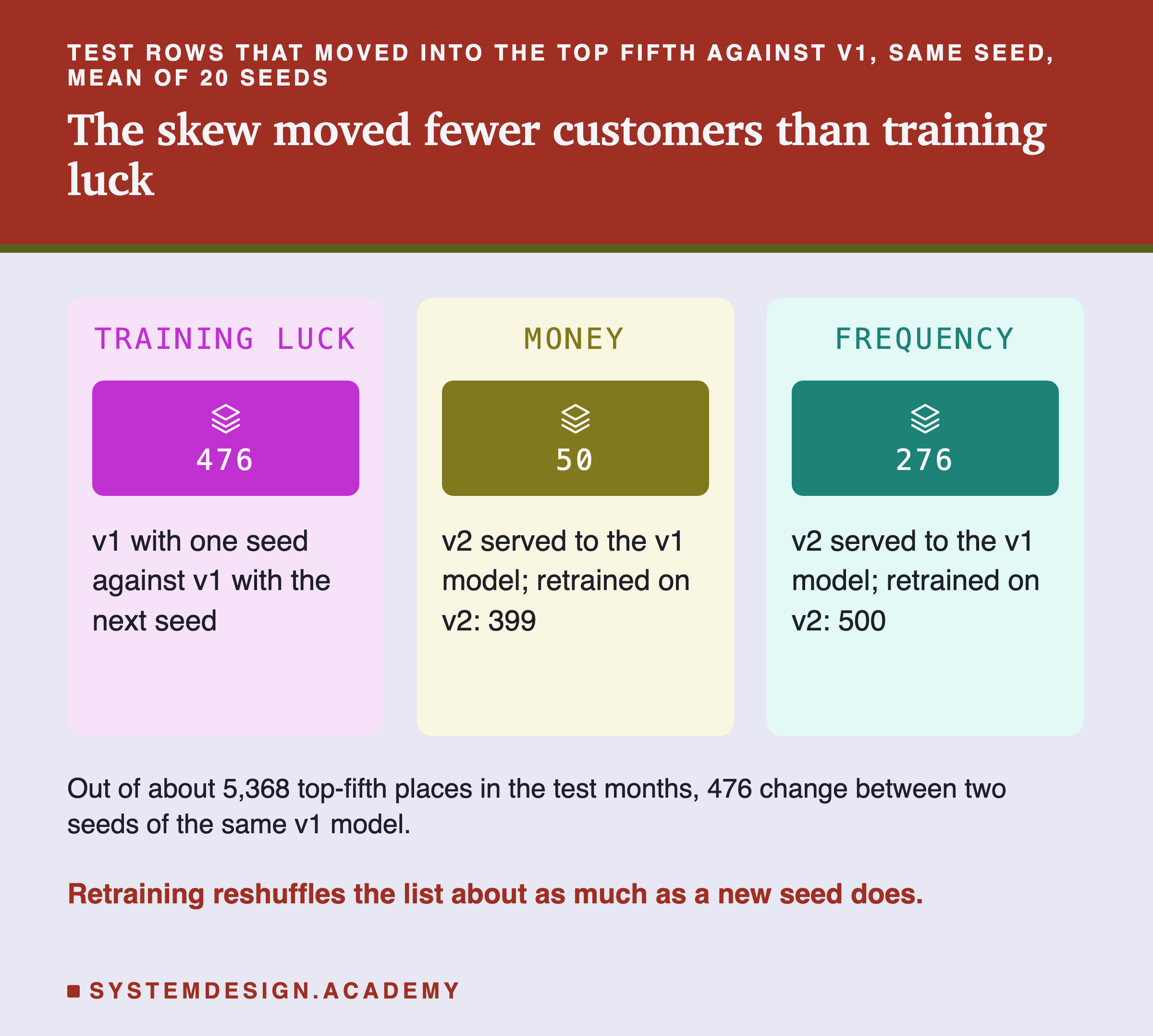
To read these counts, I need a yardstick. The top fifth of the five test months holds about 5,368 places. Train the same v1 model with one seed and then the next seed. 476 rows move into the list and 476 move out, with nothing else changed. That is training luck alone.

Against that yardstick, the money skew was tiny. On average, 50 rows moved in and 50 moved out, about 15 and 13 of them buyers. The largest change in one customer's score was 0.199, averaged over seeds. The frequency skew moved more: 276 rows in, 87 of them buyers, and 276 out, 80 of them buyers.

Retraining on v2 moved 399 rows for money and 500 for frequency. That is about what a new seed does. A retrained model is a new model, and a new model always reshuffles the edges of the list.

So if your team watches the contact list, retraining on a new definition shows up as churn. But retraining with a new seed shows up as churn too, about as much. You cannot tell those two apart by looking at the list. The silent money change, by contrast, moved only 50 rows, far fewer than a new seed.

Now scenario d: only the last k training months were redone with v2, and the older months still hold v1 in the same column.

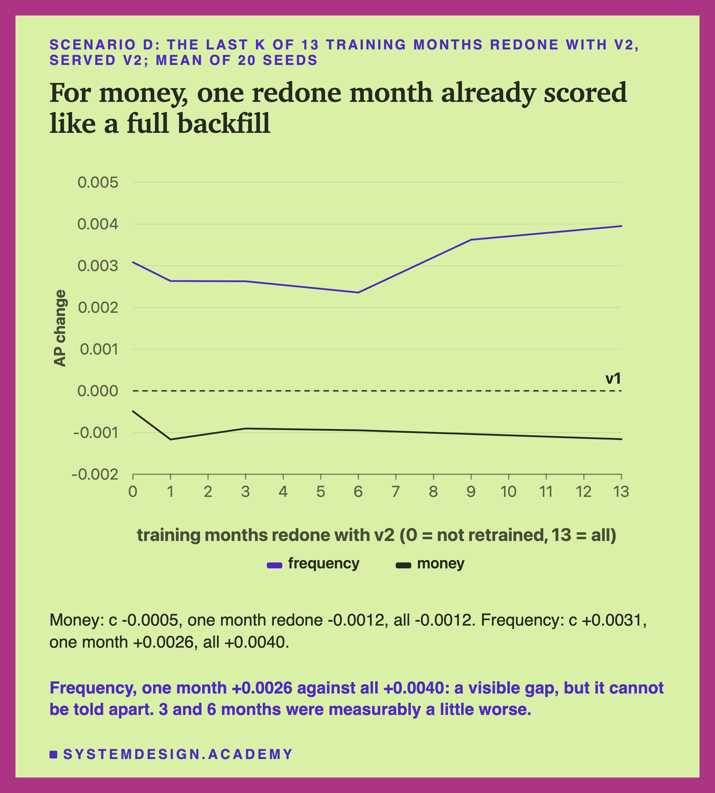
The surprise here is how little the mix mattered for money. Redoing just one month, the newest, already gave the same score as a full backfill: -0.0012 in both cases. No mixed version could be told apart from the full one. For frequency, 1 and 9 redone months could not be told apart from the full backfill, although one month, +0.0026, sits visibly below all thirteen, +0.0040. But 3 and 6 months were measurably a little worse: by 0.0013 and 0.0016.

One possible reason, which I did not test: the newest months hold the most rows. The last month has 4,607 and the first only 1,802, so the newest months weigh most in training.

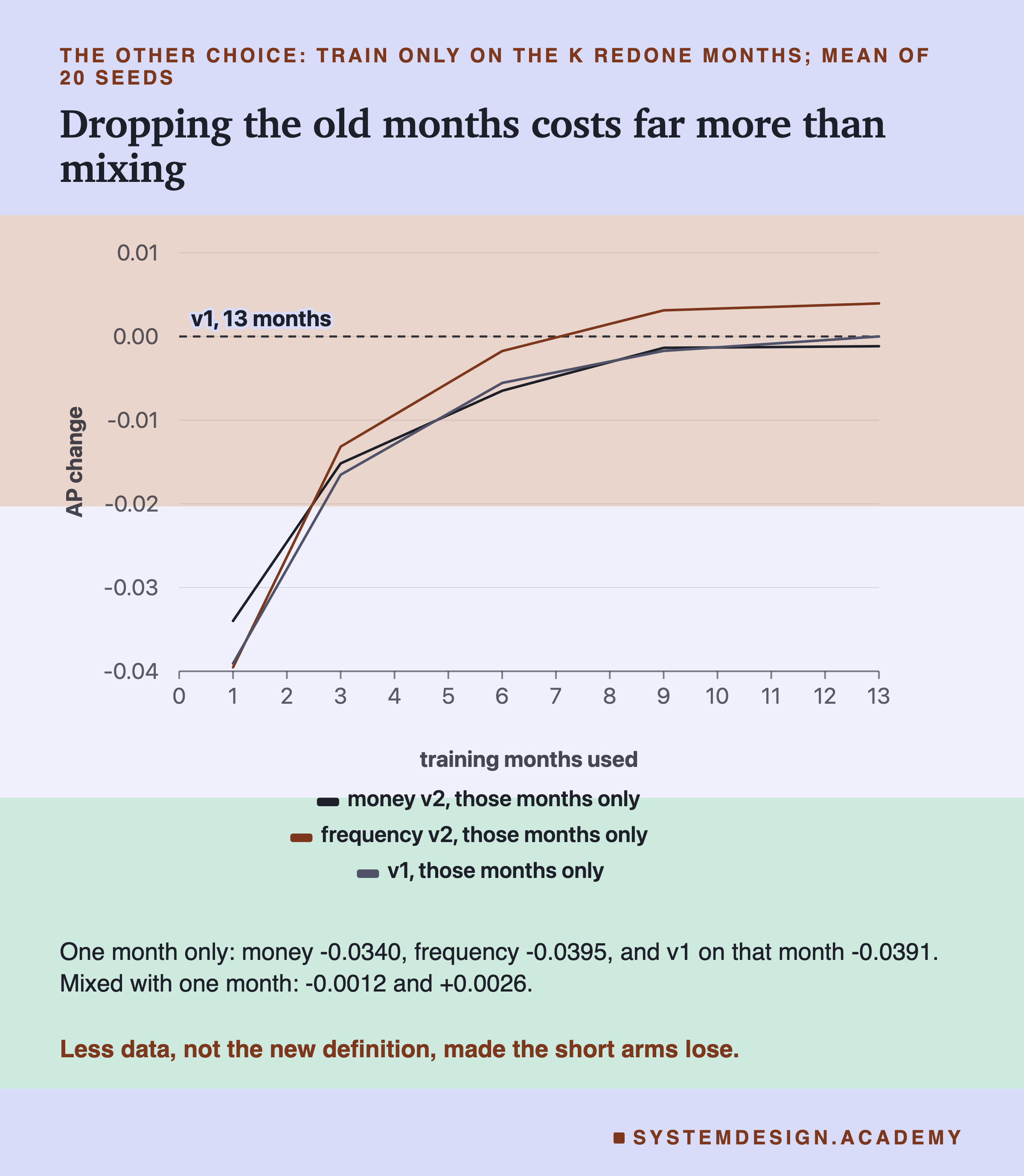
The other choice, drop, trains only on the redone months. This was much worse. Trained on one v2 month only, money lost 0.0340 and frequency 0.0395. With 3 months, they lost 0.0152 and 0.0132. Mixing beat dropping by a wide margin: at one month, by 0.0327 for money and 0.0421 for frequency, both measurable. At 9 months, mixing and dropping could not be told apart.

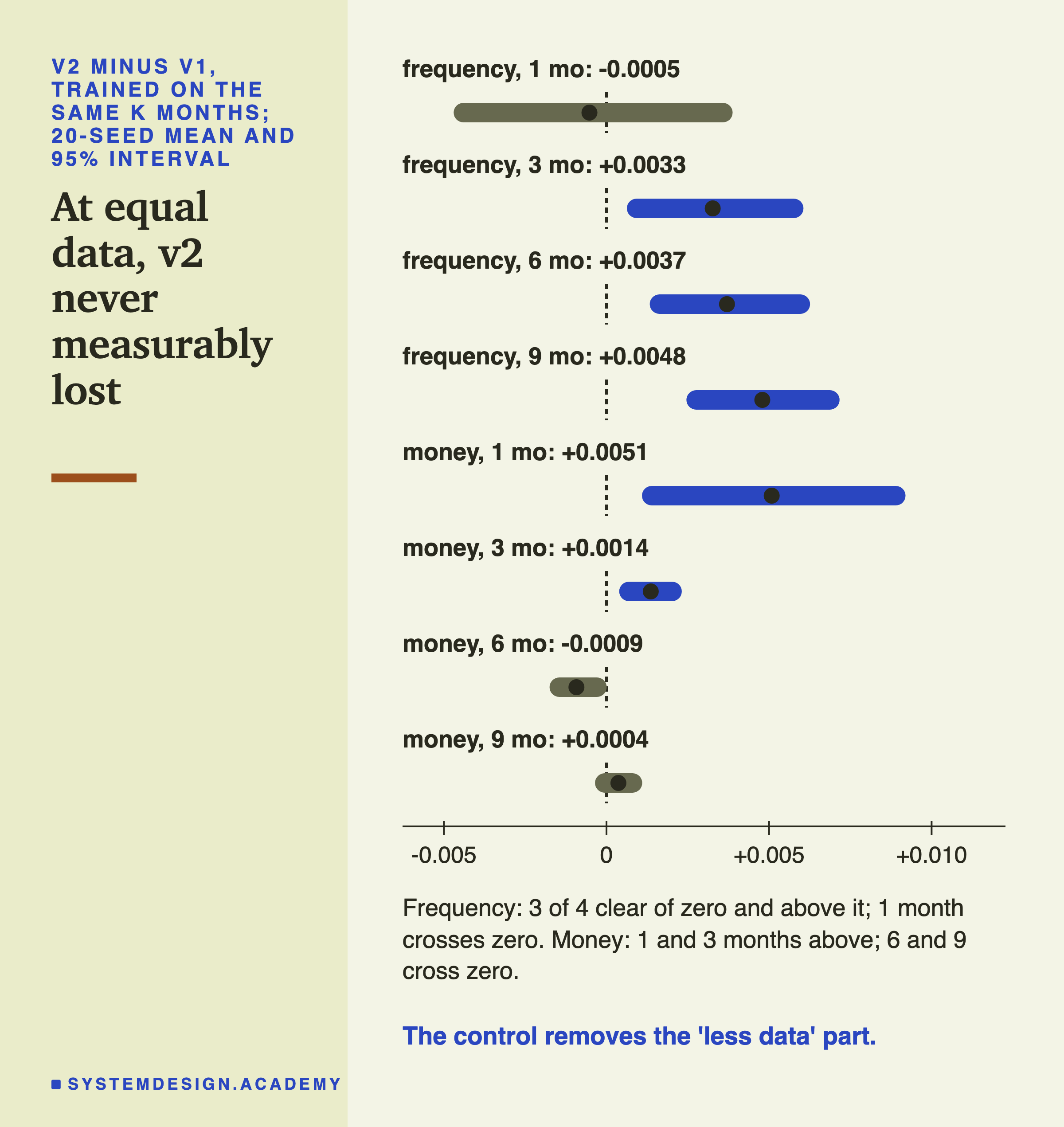
But was it v2 that hurt the drop arms, or just having less data? The control answers that. Trained on v1, on the same one month, the model lost 0.0391, about the same as the drop arms.

Now the question that matters most in practice. Could anything have noticed the change?

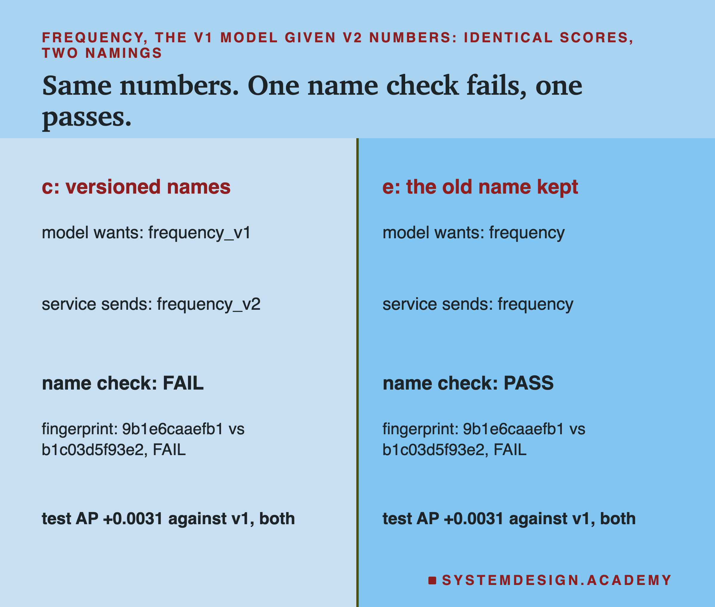
In scenario c, the names carry the version. The model was trained on frequency_v1, so it stores that name. The service now sends frequency_v2. A name check fails, and a careful service would refuse to score until someone retrains or rolls back. In scenario e, both sides say frequency, and the name check passes. The model gets exactly the same numbers in both scenarios.

The fingerprint check catches both. The model stores a short code computed from each column's definition text: 9b1e6caaefb1 for the v1 frequency rule. The service computes the same code from the rule it uses: b1c03d5f93e2 for v2. They differ, so the check fails, whatever the column is called.

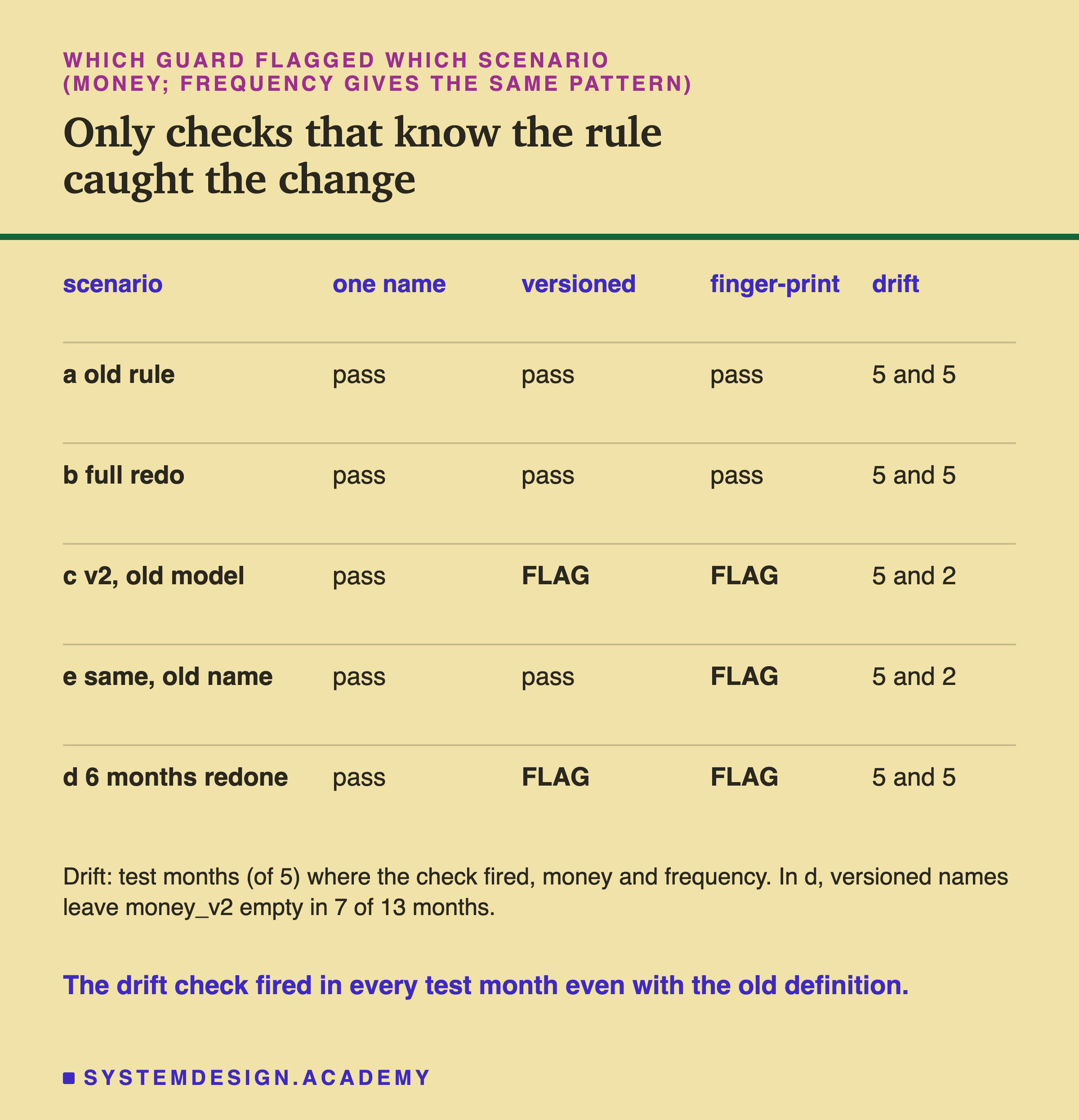
The table puts all the checks together. With one plain name, nothing ever fails. With versioned names, c fails, and so does the half-done backfill d. In d, a versioned pipeline cannot store two rules in one column. So exists only in the redone months: 57.3 percent of the training rows when 6 months were redone. That empty space is easy to see and easy to test. The fingerprint check flags c, e and d.

Many teams watch their features with a drift check. It compares the numbers being served now with the numbers the model was trained on, and raises an alarm when they look too different. If it worked, it would catch a definition change without any names or fingerprints.

I used the population stability index, or PSI. First, cut the training values into up to ten groups at their deciles; for frequency, many customers share the same count, and those ties leave six unequal groups. Then count what share of the served values falls into each group. If the shares match, PSI is near zero. The more they differ, the larger it gets.

A common rule of thumb says PSI below 0.10 is little change, 0.10 to 0.25 moderate, and 0.25 or more significant. Yurdakul and Naranjo (2020, Journal of Risk Model Validation) give it, attribute it to Lewis (1994), and note it is used without any known error rates. So I set my own alarm from the valid months instead: the largest PSI that v1 showed in the three valid months, April to June 2011. A test month fires when its PSI is higher.

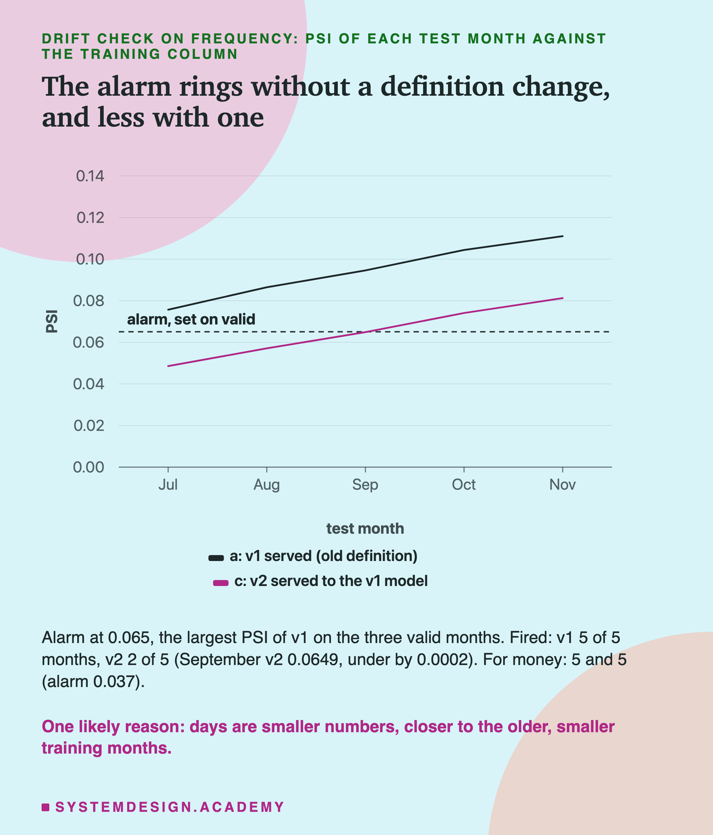
The drift check fired in all 5 test months with no definition change at all, for both money and frequency. For money, it also fired in all 5 months under the real change, so it could not tell the two apart. For frequency it fired in only 2 of 5 months under the real change, less often than with no change. One of those misses was close: in September, v2 scored 0.0649 against an alarm of 0.0651.

The training-side version of the check was no better. For the half-done backfill, I compared each training month with the month before. The month where v1 switched to v2 never fired, for any k, for either change. For money with 6 months redone, the switch scored 0.0085 against an alarm of 0.0091.

Serving frequency v2 to the v1 model raised AP in all 20 seeds. I asked one question about it after the results, labelled as such: where does the change come from?

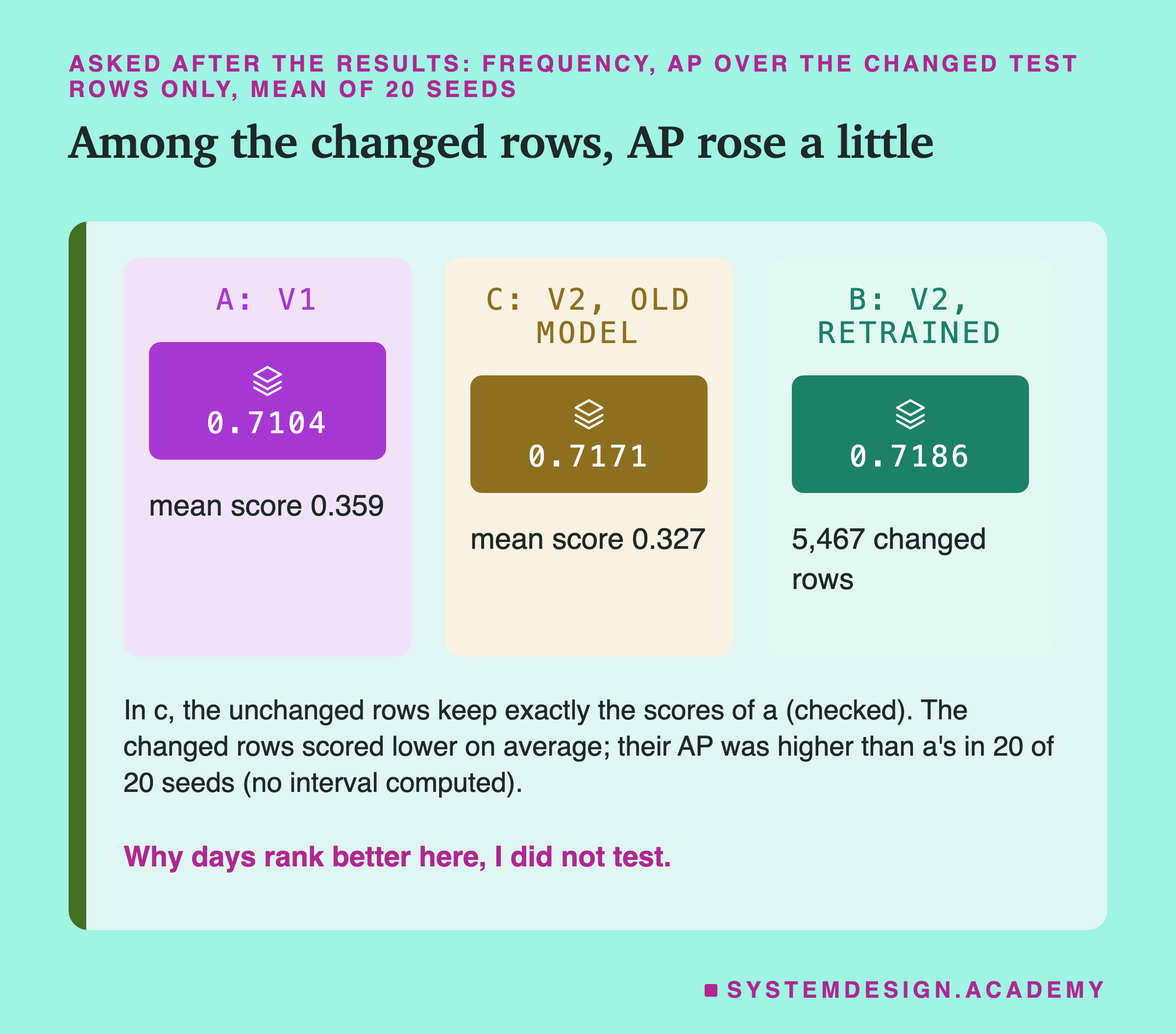
In scenario c only the 5,467 changed rows get new inputs. Every other row gets exactly the same input as in a, so exactly the same score, and the lab checks that. So the whole effect comes from the changed rows: where they land, and how they are ordered among themselves.

Their mean score fell, from 0.359 to 0.327, because fewer "orders" makes a customer look less active. Yet their AP, counted among themselves only, rose from 0.7104 to 0.7171, in 20 of 20 seeds. I did not compute an interval for this, so read it as a direction only. One possible reason, which I did not test: two invoices on one day may often be one shopping trip split in two. If so, days are a cleaner count of visits.

I want to be careful here. This does not mean a silent definition change is safe. It means this particular change, on this shop, happened to point in a good direction. The money change pointed the other way. Nobody could have known which way before measuring.

I wrote seven guesses into the lab before it ran. Here they are against the results.

1. "money b vs a: cannot be told apart from zero." Wrong. Retrained on v2, money was measurably worse, by 0.0012.

2. "money c (= e) vs a: a small loss, close to lesson 5's -0.000490, measurable." Right: -0.0005, interval clear of zero.

3. "frequency: fewer rows change than for money; I guess about 15% of test rows. ... c loses more than money's c: between -0.002 and -0.01." Half right. Fewer rows changed, 5,467, but that is 20.4 percent, not 15. And c did not lose; it gained 0.0031.

4. "frequency b vs a: cannot be told apart from zero." Wrong. It gained 0.0040.

5. "d_k: the loss shrinks as k grows, and d_9 cannot be told apart from b. d_k beats drop_k at k = 1 and 3 (drop has much less data); at k = 9 they cannot be told apart." Mostly right on the comparisons, wrong on the shape. For money, one redone month already scored like a full backfill, so nothing shrank as k grew.

6. "top fifth: c moves hundreds of rows per seed for frequency and fewer than 200 for money, both above the seed-to-seed churn of arm a for frequency, below it for money." Half right. Money moved 50, below the churn of 476. Frequency moved 276: hundreds, but below the churn, not above.

7. "drift check: it fires on frequency c in all 5 test months and on money c in at least 3; arm a fires 0 times." Wrong where it mattered. It fired on frequency c in only 2 months, and on unchanged a in all 5.

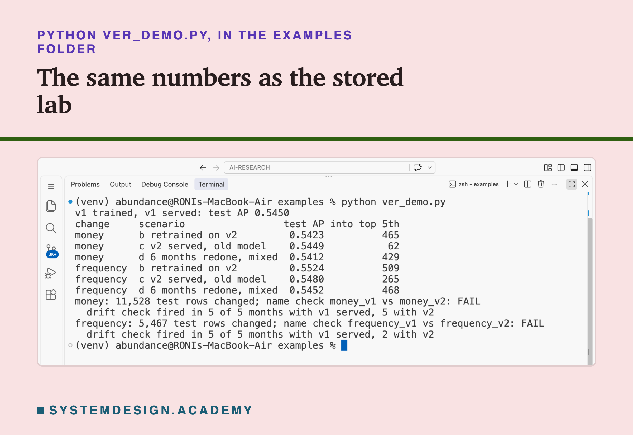
The full lab trains 25 model arms for each of 20 seeds. I wrote a small demo that does one slice of it, with seed 0.

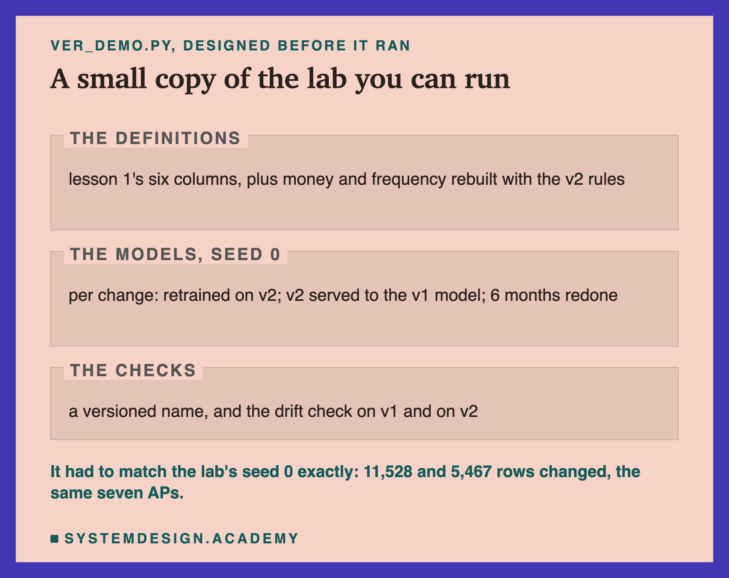
I wrote the demo's design into its docstring after the lab had run and before the demo first ran. Its code builds the two v2 columns in its own short way, so it is also a second check of the lab's seed 0.

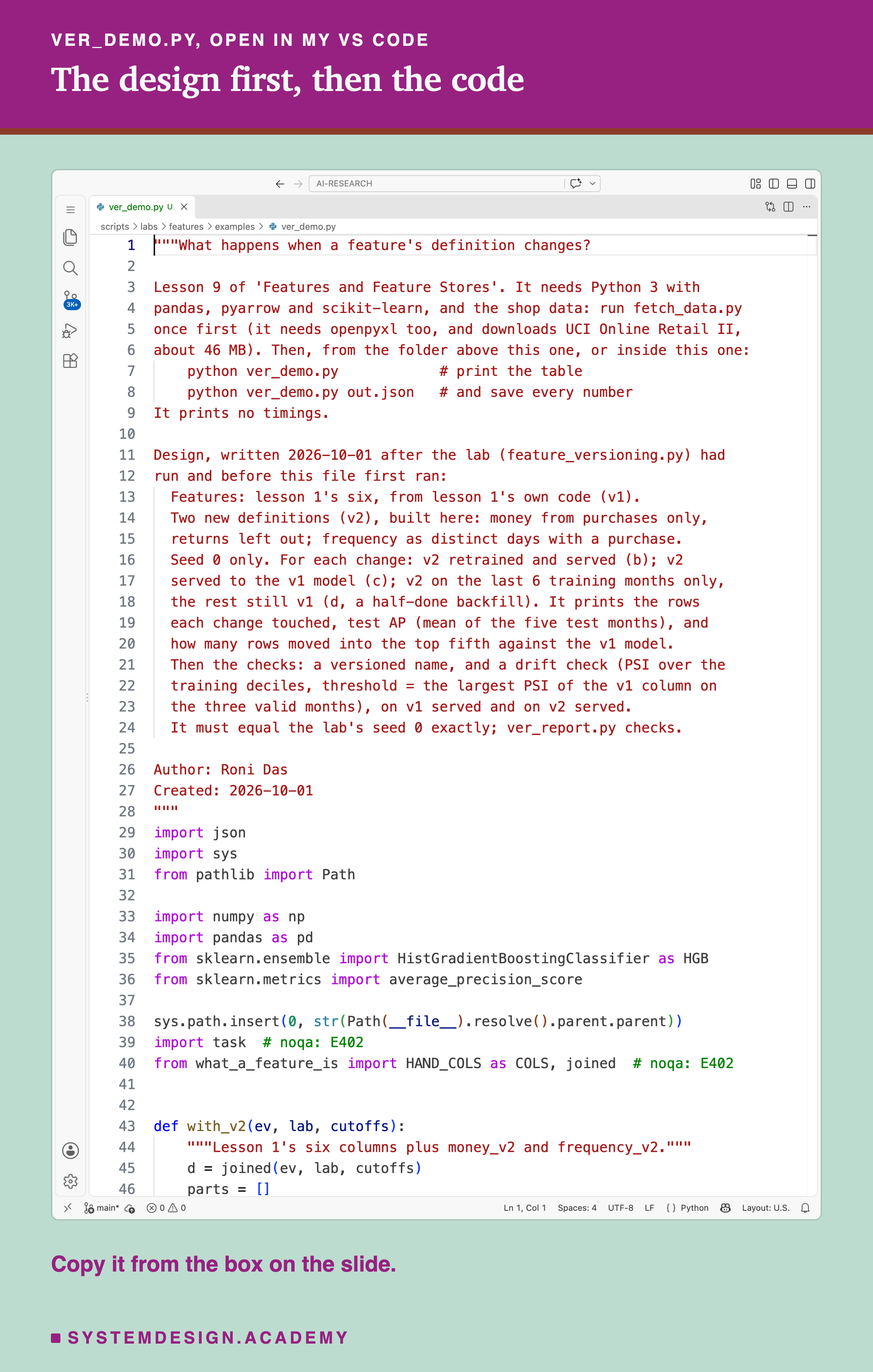
Before you run this lab. You need Python 3 with pandas, pyarrow and scikit-learn: pip install pandas pyarrow scikit-learn openpyxl. First run python fetch_data.py from the scripts/labs/features folder. It downloads the shop data once, about 46 MB, and writes one cleaned file.

The demo imports lesson 1's lab file, what_a_feature_is.py, and task.py from that same folder. It needs no GPU. I ran it with scikit-learn 1.9.1 and pandas 3.0.6 on a Mac. These libraries run on Windows and Linux too, but I have not checked the numbers there. Give it a file name, python ver_demo.py out.json, and it also saves every number. That is how results/ver-demo.json was made.

"""What happens when a feature's definition changes?

Lesson 9 of 'Features and Feature Stores'. It needs Python 3 with
pandas, pyarrow and scikit-learn, and the shop data: run fetch_data.py
once first (it needs openpyxl too, and downloads UCI Online Retail II,
about 46 MB). Then, from the folder above this one, or inside this one:
    python ver_demo.py            # print the table
    python ver_demo.py out.json   # and save every number
It prints no timings.

Design, written 2026-10-01 after the lab (feature_versioning.py) had
run and before this file first ran:
  Features: lesson 1's six, from lesson 1's own code (v1).
  Two new definitions (v2), built here: money from purchases only,
  returns left out; frequency as distinct days with a purchase.
  Seed 0 only. For each change: v2 retrained and served (b); v2
  served to the v1 model (c); v2 on the last 6 training months only,
  the rest still v1 (d, a half-done backfill). It prints the rows
  each change touched, test AP (mean of the five test months), and
  how many rows moved into the top fifth against the v1 model.
  Then the checks: a versioned name, and a drift check (PSI over the
  training deciles, threshold = the largest PSI of the v1 column on
  the three valid months), on v1 served and on v2 served.
  It must equal the lab's seed 0 exactly; ver_report.py checks.

Author: Roni Das
Created: 2026-10-01
"""
import json
import sys
from pathlib import Path

import numpy as np
import pandas as pd
from sklearn.ensemble import HistGradientBoostingClassifier as HGB
from sklearn.metrics import average_precision_score

sys.path.insert(0, str(Path(__file__).resolve().parent.parent))
import task  # noqa: E402
from what_a_feature_is import HAND_COLS as COLS, joined  # noqa: E402


def with_v2(ev, lab, cutoffs):
    """Lesson 1's six columns plus money_v2 and frequency_v2."""
    d = joined(ev, lab, cutoffs)
    parts = []
    for t in cutoffs:
        buys = ev[(ev["ts"] < t) & ~ev["is_return"]]
        g = buys.groupby("customer_id")
        parts.append(pd.DataFrame({"money_v2": g["amount"].sum(),
                                   "frequency_v2": g["ts"].apply(lambda s: s.dt.date.nunique()),
                                   "cutoff": t}).reset_index())
    d = d.merge(pd.concat(parts), on=["customer_id", "cutoff"], how="left")
    return d.fillna({"money_v2": 0.0, "frequency_v2": 0})


def x(d, change=None, rows=None):
    out = d[COLS].to_numpy(float).copy()
    if change:
        rows = np.ones(len(d), bool) if rows is None else rows
        out[rows, COLS.index(change)] = d[f"{change}_v2"].to_numpy(float)[rows]
    return out


def per_month(d, p):
    d = d.assign(p=p)
    ap = d.groupby("cutoff")[["label", "p"]].apply(
        lambda g: average_precision_score(g["label"], g["p"])).mean()
    top = d.groupby("cutoff")["p"].rank(ascending=False, pct=True) <= 0.2
    return ap, top.to_numpy()


def psi(train, serve):
    edges = np.unique(np.quantile(train, np.linspace(0.1, 0.9, 9)))
    a = np.bincount(np.searchsorted(edges, train), minlength=len(edges) + 1) / len(train)
    b = np.bincount(np.searchsorted(edges, serve), minlength=len(edges) + 1) / len(serve)
    a, b = np.maximum(a, 1e-4), np.maximum(b, 1e-4)
    return float(((b - a) * np.log(b / a)).sum())


ev = task.load_events()
lab_tr, lab_va, lab_te = task.splits(ev)
tr = with_v2(ev, lab_tr, task.TRAIN_CUTOFFS)
va = with_v2(ev, lab_va, task.VALID_CUTOFFS)
te = with_v2(ev, lab_te, task.TEST_CUTOFFS)
last6 = (tr["cutoff"] >= task.TRAIN_CUTOFFS[-6]).to_numpy()
y = tr["label"]

v1_model = HGB(random_state=0).fit(x(tr), y)
ap_a, top_a = per_month(te, v1_model.predict_proba(x(te))[:, 1])
out = {"changed": {}, "arms": {"a": {"ap": ap_a, "moved_in": 0}}, "fires": {}}
print(f"v1 trained, v1 served: test AP {ap_a:.4f}")
print(f"{'change':10s} {'scenario':24s} {'test AP':>7s} {'into top 5th':>12s}")
for ch in ("money", "frequency"):
    out["changed"][ch] = int((te[ch] != te[f"{ch}_v2"]).sum())
    arms = {"b": HGB(random_state=0).fit(x(tr, ch), y),
            "c": v1_model,
            "d_6": HGB(random_state=0).fit(x(tr, ch, last6), y)}
    names = {"b": "b retrained on v2", "c": "c v2 served, old model",
             "d_6": "d 6 months redone, mixed"}
    for k, m in arms.items():
        ap, top = per_month(te, m.predict_proba(x(te, ch))[:, 1])
        moved = int((top & ~top_a).sum())
        out["arms"][f"{ch}/{k}"] = {"ap": ap, "moved_in": moved}
        print(f"{ch:10s} {names[k]:24s} {ap:7.4f} {moved:12d}")
for ch in ("money", "frequency"):
    cut_va, cut_te = va["cutoff"].to_numpy(), te["cutoff"].to_numpy()
    t1 = tr[ch].to_numpy(float)
    limit = max(psi(t1, va[ch].to_numpy(float)[cut_va == t]) for t in task.VALID_CUTOFFS)
    fires = []
    for col in (ch, f"{ch}_v2"):
        vals = [psi(t1, te[col].to_numpy(float)[cut_te == t]) for t in task.TEST_CUTOFFS]
        fires.append(sum(v > limit for v in vals))
    out["fires"][ch] = fires
    print(f"{ch}: {out['changed'][ch]:,} test rows changed; name check "
          f"{ch}_v1 vs {ch}_v2: FAIL")
    print(f"  drift check fired in {fires[0]} of 5 months with v1 served, "
          f"{fires[1]} with v2")
if len(sys.argv) > 1:
    json.dump(out, open(sys.argv[1], "w"), indent=1)

This box holds 58 real customers from the cutoff 1 November 2011, every 100th one by customer number. For each, it has money and frequency under v1 and v2, whether they bought, and the lab's seed-0 scores from the v1 model: given v1, given v2 money, and given v2 frequency. It needs nothing but Python, so it runs in your browser.

Press Run. It shows which customers have a new value, the AP of this small sample with v1 and with v2 served, the name check and the drift check. Then set VERSIONED = True and run again: the name check now fails. Set CHANGE = "money" to look at the other change.

The report script writes this box from the lab's stored results. It checks that the box's AP, written in plain Python, equals scikit-learn's on the same rows, and that its PSI equals a numpy version, for both changes and both namings. Please notice one thing when you run it: with only 58 customers, the drift check is very noisy. Its PSI on this sample is several times the alarm level, even for v1. A drift check needs many rows before its number means anything.

The lab is one file, scripts/labs/features/feature_versioning.py. It imports lesson 1's feature code instead of copying it, so scenario a is exactly lesson 1's model, and the lab checks that on all 20 seeds.

v2_columns builds the two new columns for every customer at every cutoff. It takes only the lines before the cutoff, keeps the purchase lines, and adds up their amounts for money v2. For frequency v2 it counts the distinct calendar days of those lines. It also records whether the customer made any return, so the lab can check that money changed exactly those rows.

matrix builds the six columns the model sees, in lesson 1's order. For a chosen change, it swaps in the v2 value on chosen rows: all rows for a full backfill, or only the last k months for a partial one. arm_specs lists every arm by four facts: which change training uses, which rows hold v2, which months training keeps, and which change serving uses. fit_arm turns one spec into a trained model and its test scores.

checks runs the three guards. The name and fingerprint checks compare strings. The drift check calls psi, which cuts the training values at their deciles and compares shares. data_facts counts the changed rows and their size.

main trains every arm for every seed, records AP, the top-fifth moves and the score changes, and runs the paired bootstrap. holds the two post-results questions.

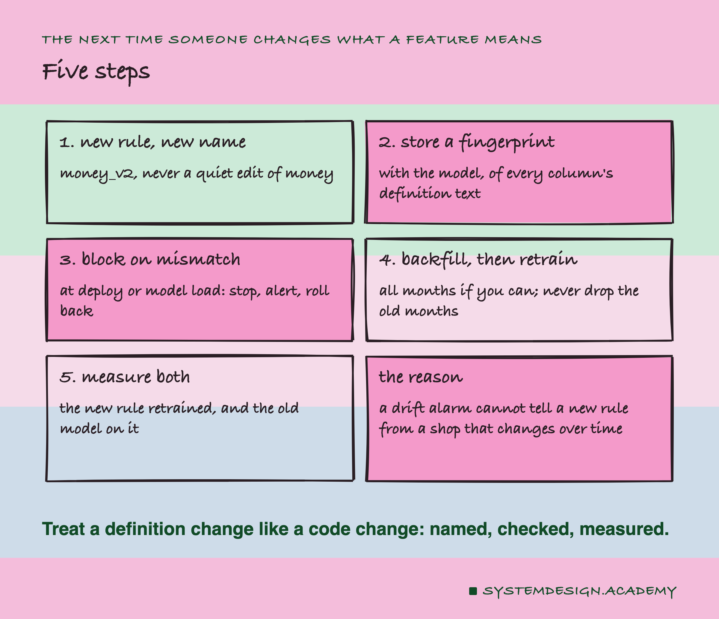
These are the steps I would take the next time a feature's meaning changes.

1. Give the new rule a new name. Write money_v2 next to money_v1. Never edit the code behind money and keep the name. In this lab, the plain name hid every scenario from the name check.

2. Store a fingerprint of every definition with the model. A short hash of the definition text, saved next to the trained model. At serving, compute the same hash and compare. It flags every change here by construction, including the silent one.

3. Block a mismatch before it serves. Run the check when a model is deployed or loaded, not on every request. If the model was trained on money_v1 and the store only has money_v2, stop the deploy, alert someone, and roll back to the last good pair. A check that only logs a warning is easy to miss.

4. Backfill before you retrain, and keep the old months. If the backfill cannot finish, training on the mix was far better here than throwing old months away. But check the mix, because for frequency, 3 and 6 redone months were a little worse than a full backfill.

5. Measure both the new rule and the skew, with seeds. The two changes here went in opposite directions. Only measuring told me which.

6. Do not rely on a drift alarm against a fixed training reference to catch a definition change. Here it fired on every feature without any definition change, and the change itself was far smaller than the drift from time.

Use versioned names and fingerprints whenever a feature is read by a model you cannot retrain at the same moment as you change the feature. That is almost always true when a separate team owns the feature pipeline, or when several models read the same feature.

Use a full backfill when the new definition can be computed from data you still have. Here the raw invoices were all kept, so every month could be redone. If the raw data is gone, you cannot backfill, and data versioning is the lesson about keeping it.

A partial backfill is acceptable if you measure it. Here, mixing worked about as well as a full backfill for money, and a little worse for frequency at 3 and 6 months.

Versioning is less useful for a one-person project where one script computes the feature and trains the model together, every time. There the code is the version. Even then, a fingerprint saved with the model costs one line.

Never use a drift alarm against a fixed training reference as your only guard. In this lab it could not tell a new definition from an ordinary month.

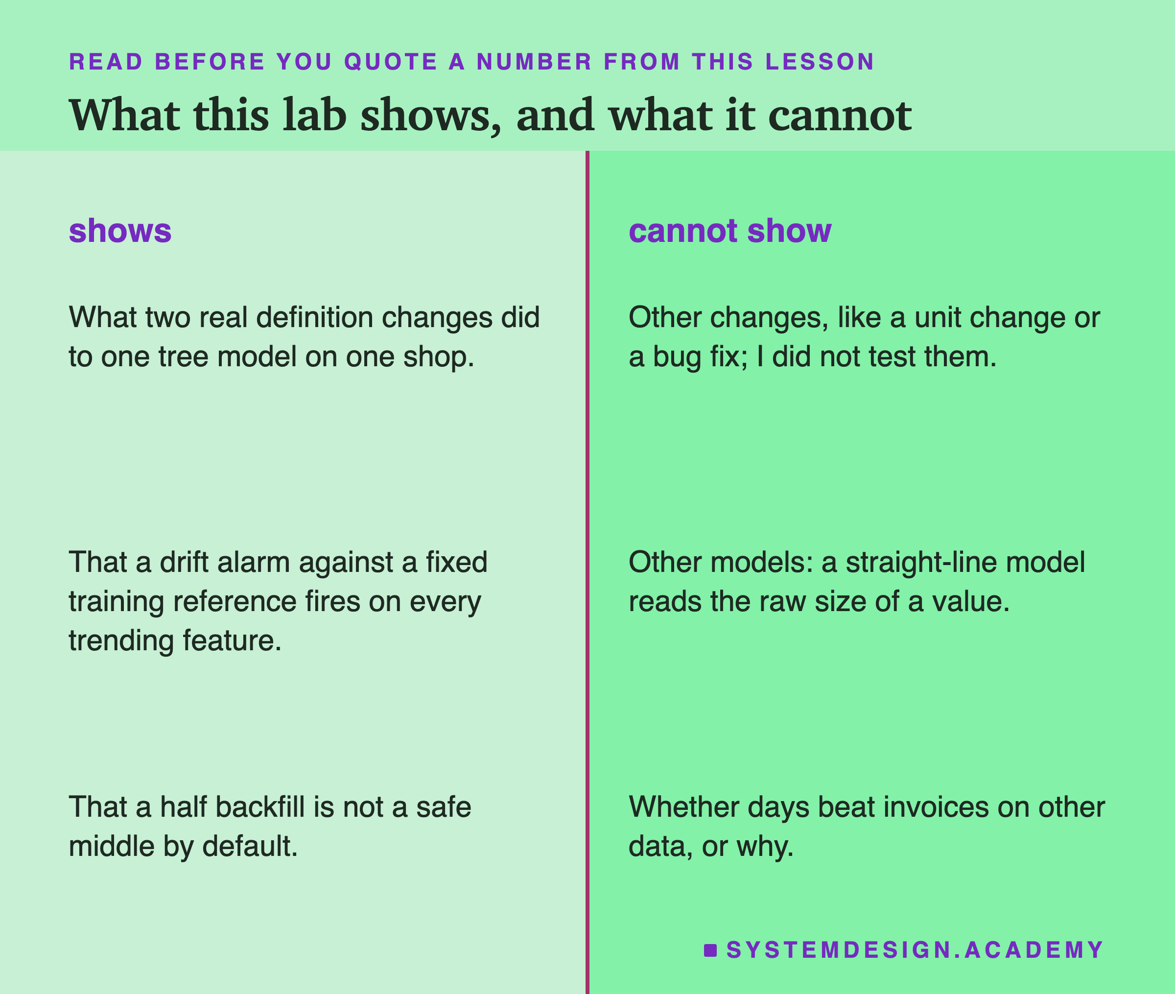
Two changes, both chosen by me. Both v2 rules are fair readings of the same idea, and they mostly keep the order of values: rank correlation 0.986 to 0.990, measured in the reviewer check. A change that moves values far from what the model learned, like a unit change from pounds to pence, or a bug that scrambles them, could do much more harm. I did not test one.

One tree model. The model sorts each column into bins and only sees the bin. A change that keeps a customer in about the same place in the ranking barely moves the score. A straight-line model uses the raw size of each value, so customer 12346's jump from minus £64.68 to £77,556.46 could matter far more there.

One shop, and a shift between periods. The training months had a higher buy rate than the test months, 23.4 percent against 19.7 percent. Every scenario shares that shift, so it does not favour one over another, but it limits how far the numbers carry.

The drift check is one rule among many. I set its alarm on the valid months. Another threshold, or a check that compares against the most recent months instead of the training months, could behave differently. I did not test one.

Labelled additions. Two questions were asked after I saw the results, and both are labelled in the lab and here: the medians per month, and AP on the changed rows. I report no timings.

If you take one thing from this lesson to work on Monday, make it this. Go to your feature code, and find every feature that a model reads. For each one, ask: if someone changed the rule behind this name tomorrow, what would notice? If the honest answer is "a drift dashboard", this lab says that may not be enough.

Then add the cheapest guard first. Save a fingerprint of each feature's definition next to the model when it is trained, and compare it when the model is loaded. It is a few lines of code, and in this lab it flagged every scenario, by construction.

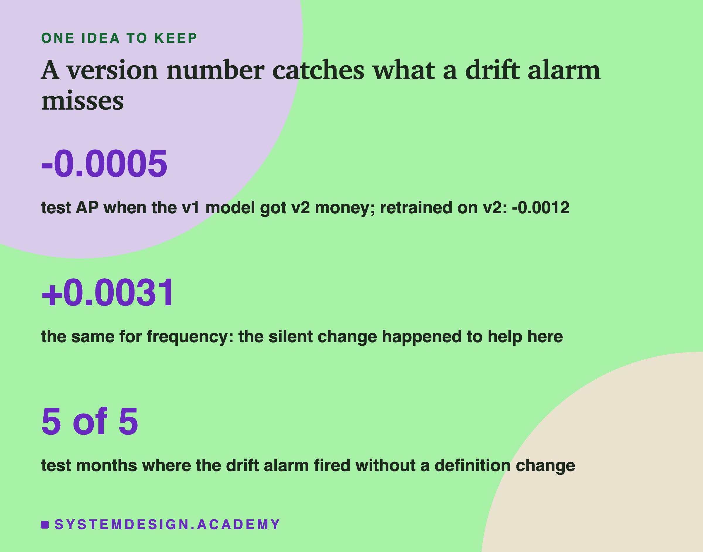
The one idea to keep: a feature's name is not its meaning. When the rule behind a name changes, the numbers can move the score either way, and a check on the numbers alone may not see it. Name the new rule, store its fingerprint with the model, and measure before you trust it.