Let me start with a small picture from a shop.

Two people work in the same small shop. At the end of each day, the first one takes the pile of paper receipts and adds them up with a pen. The second one keeps a number on her phone, and every time a sale happens she adds it at once. Both are careful. Both follow the same instruction: "keep the total of today's sales".

Will their totals agree at closing time? Usually, yes. But think about the small questions the instruction does not answer. Does a sale made at exactly closing time count today or tomorrow? Is "today" judged by the shop's clock or by the bank's clock in another country? When a customer brings something back, do you subtract it from the total or leave it out? Each person can answer those questions in a sensible way, and still get a different number from the other.

Nobody made a mistake. They simply made different, reasonable choices.

Machine learning teams have exactly this situation, every day. In this lesson I build the two people in code, give them the same instruction, and measure how often they disagree and whether it matters.

This lesson uses the same shop, the same customers and the same question as the rest of the chapter. If any of that is new, please read what a feature is first. It sets up the data and the task, and it built six simple features that I use again here: recency, frequency, money, return share, tenure and products.

An earlier lesson, train/serve skew, already showed what happens when the input at serving time is simply wrong. Its examples were temperatures in Fahrenheit instead of Celsius, and every hour shifted by five. Those were broken inputs, and they did a lot of damage.

This lesson asks a harder and more common question. What if neither side is broken? What if both pieces of code are correct readings of the same definition, written by careful people, and they still disagree in small ways? Is that harmless, or does it quietly cost something?

The lesson on point-in-time joins made sure no feature sees the future. Every feature here, on both sides, uses only events before the cutoff, and the code checks it.

Please read this slide slowly if any word is new. Every slide after it uses these words.

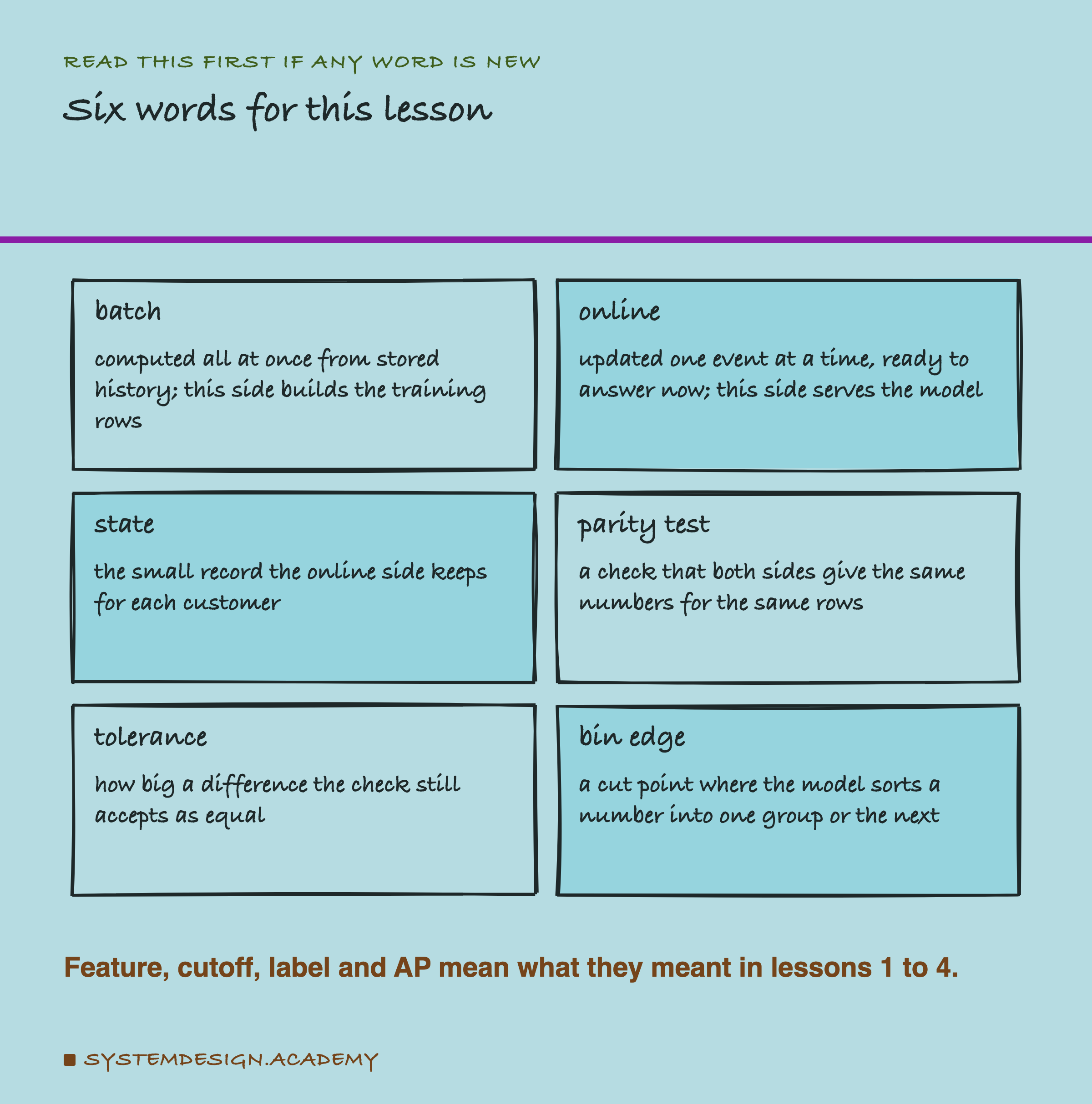
Batch means computed all at once, from all the history that is stored. Think of the man adding up a pile of receipts. In this lesson the batch side is lesson 1's pandas code, and it builds the rows the model learns from. People also call this side offline.

Online means updated one event at a time, so that an answer is ready right now. Think of the woman with the phone. The online side is what a live app would ask when it needs a prediction. A program that reads events one by one as they arrive is often called a stream processor.

State is the small record the online side keeps for each customer: when they were last seen, how much they have spent so far, and so on. Each new event changes the state a little.

A parity test is a check that the two sides give the same numbers for the same rows. "Parity" just means "being equal". A tolerance is how big a difference the check still accepts as equal. A bin edge is explained on its own slide later.

Two more words. A floating-point number is how a computer stores a number with a decimal point. It is often a tiny bit off: 0.1 is stored as a number very close to 0.1, but not exactly 0.1. UTC is the world's reference clock. London uses UTC in winter, which is called GMT, and one hour ahead of UTC in summer, which is called British Summer Time or BST.

Feature, cutoff, label, average precision (AP), seed and bootstrap mean what they meant in lessons 1 to 4. I explain the bootstrap again where it matters.

Why would anyone compute the same feature twice? Because training and serving want different things.

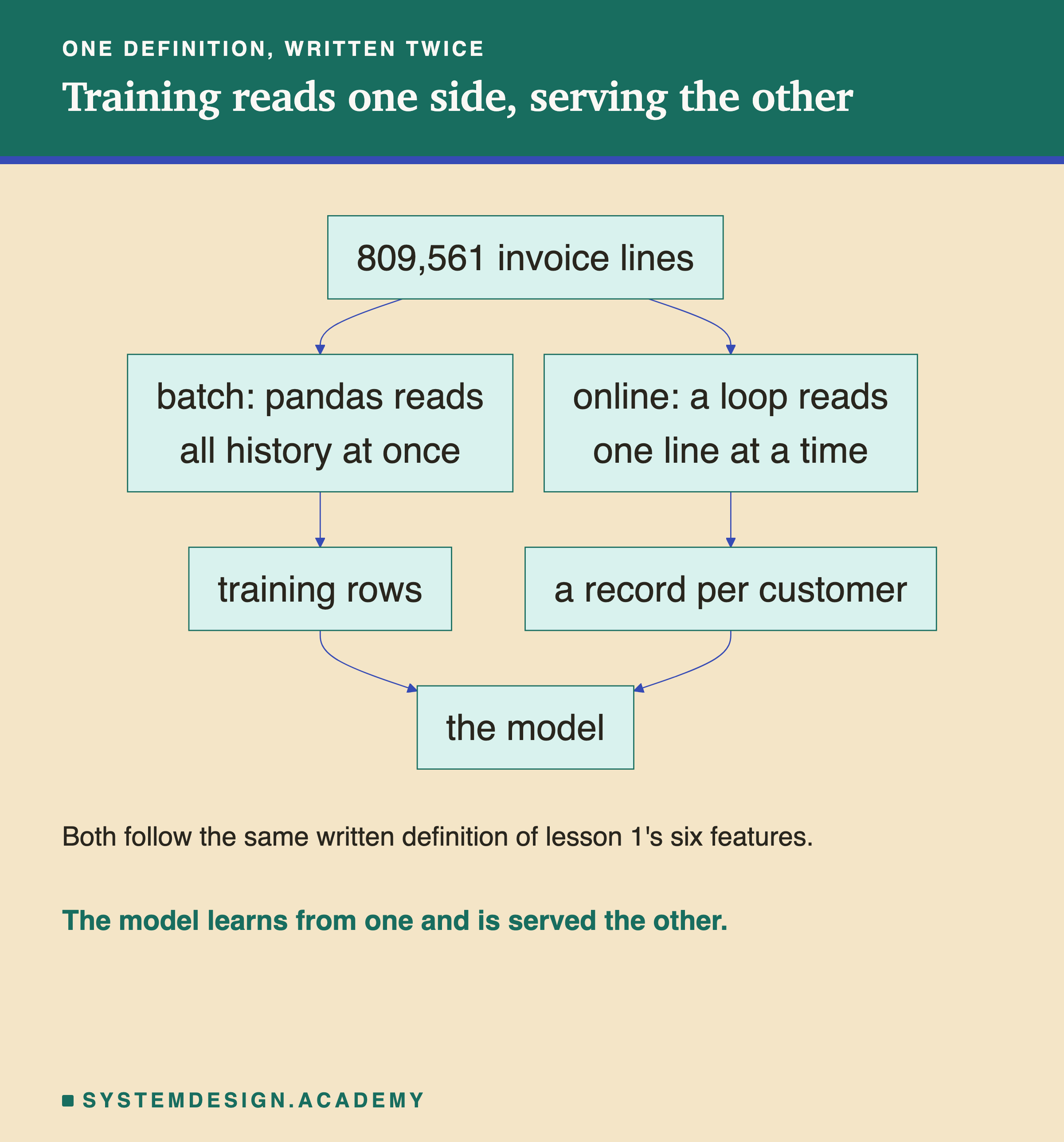
For training, you need features for thousands of customers at many past dates. Reading all the history at once, with a tool like pandas or SQL, is the natural way. Speed per customer does not matter much, because the job runs at night.

For serving, a live app asks about one customer, now, and wants the answer in a few milliseconds. Reading two years of history for every request is far too slow. So teams keep a running record for each customer and update it as each event arrives. When a request comes, the answer is already there.

So the same definition, "money is the customer's total spend", gets written twice, in two styles, often by two different people. Feature stores offer ways to help.

Feast is an open-source feature store. Its online store holds, in its own documentation's words, "only the latest feature values" for each customer. It loads them from the offline data with a step it calls materialization. Feast also has on-demand feature views, Python code that, as its documentation says, "is executed in both the historical retrieval and online retrieval paths". That is one way to avoid writing a definition twice. But a team may still compute some features in a separate stream processor, and that is the case this lesson measures.

Here is one real customer, number 12349, at the cutoff 1 July 2011. Lessons 1 and 4 used the same customer, so you can compare.

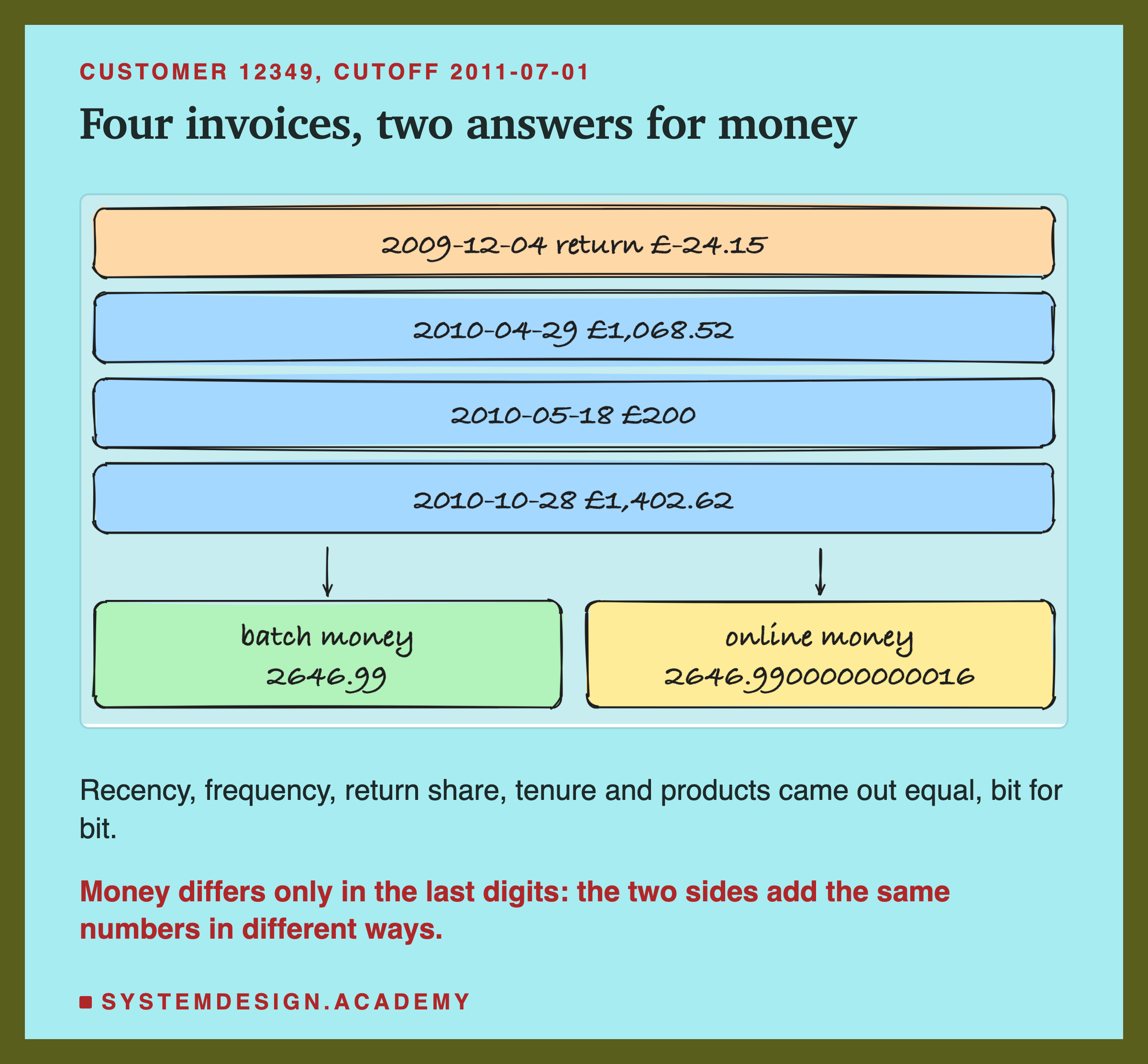
Before that date, this customer had four invoices. The first one was a return. The other three were purchases, the last one 245.65 days before the cutoff. The first line of all was 573.47 days before it.

I computed the six features both ways. Five of them came out exactly equal, down to the last bit the computer stores. Money did not. The batch side said 2646.99. The online side said 2646.9900000000016.

That tiny tail is not a bug in either piece of code. Both added the same 107 invoice lines, in the same order. They just added them in different ways, and a later slide explains how. For now, notice what this means for a test: if you check "are the two numbers equal?", the correct online code already fails.

The online side is a plain Python loop. I wrote it from the definitions in lesson 1, not by copying the pandas code, because that is how a second team would write it.

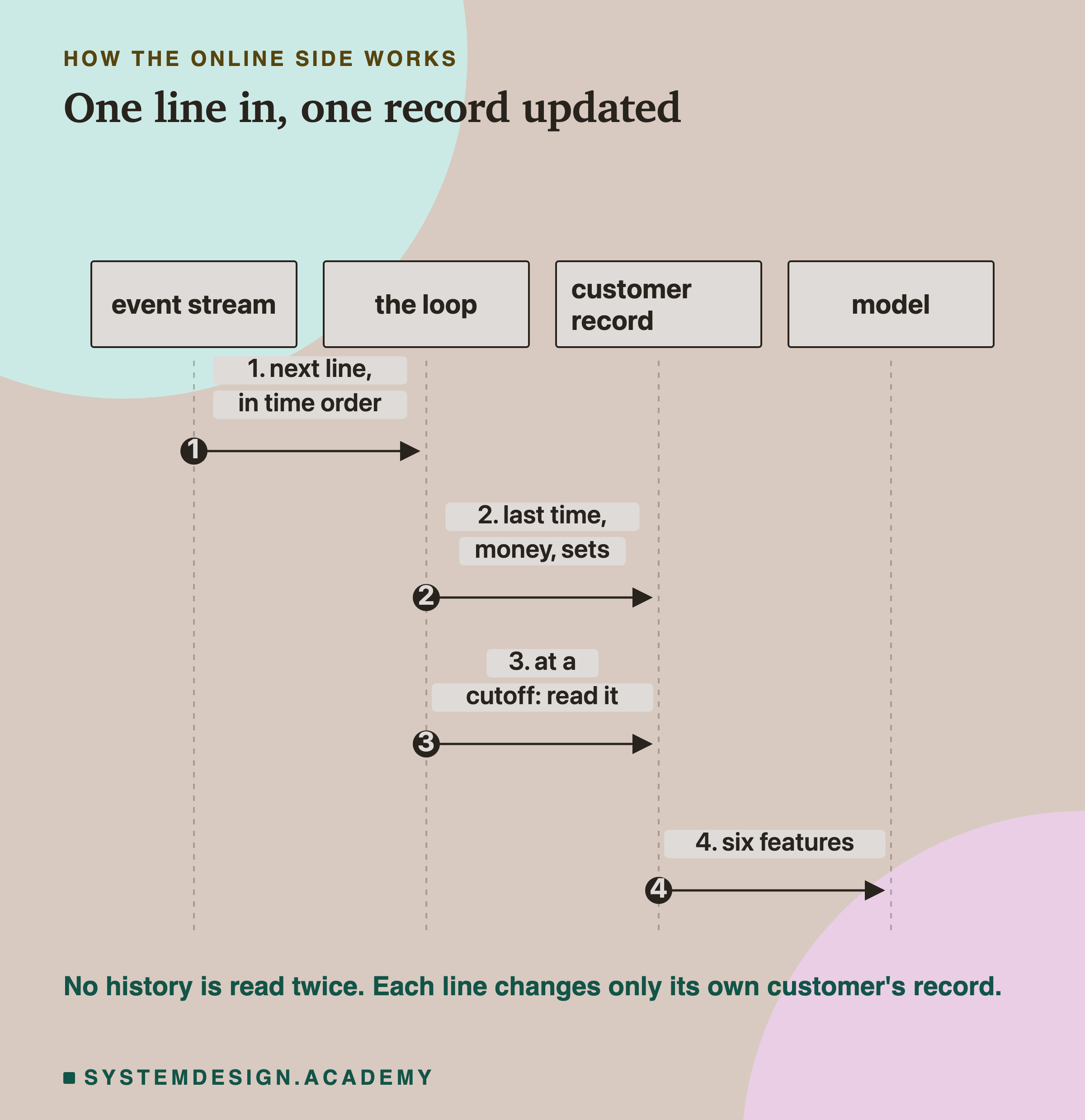
The loop reads the 809,561 invoice lines in time order, once. For each line it finds that customer's record, and changes it. It sets "last seen" to this line's time. It adds the line's amount to money. If the line is a purchase, it adds the invoice number to a set of invoices, and the product code to a set of products. A set is a collection that keeps each item only once, so its size counts different things. It also counts lines and return lines.

When the stream reaches a cutoff, the loop stops and reads every customer's record, the way a live service would answer a request at that moment. Recency is the cutoff minus "last seen". Tenure is the cutoff minus "first seen". Frequency is the size of the invoice set, and so on.

Nothing in this loop ever looks back at old lines. That is what makes it fast enough for serving. It is also what makes small choices matter, because each choice is baked into the record as the events go by.

I wrote the lab's design into the docstring of scripts/labs/features/online_offline.py before it first ran. Lessons 1 to 4 had run, and I had read their results. No model had been trained for this lesson.

Before writing the design I checked a few facts about the data, because they decide what some choices can do here. No invoice line sits at midnight: the shop's lines run from 06:00 to 21:59, London time. 65 of the 44,876 invoices have lines stamped one or two minutes apart; every other invoice has one time. 275 of the 5,942 customers have a return as their very first line.

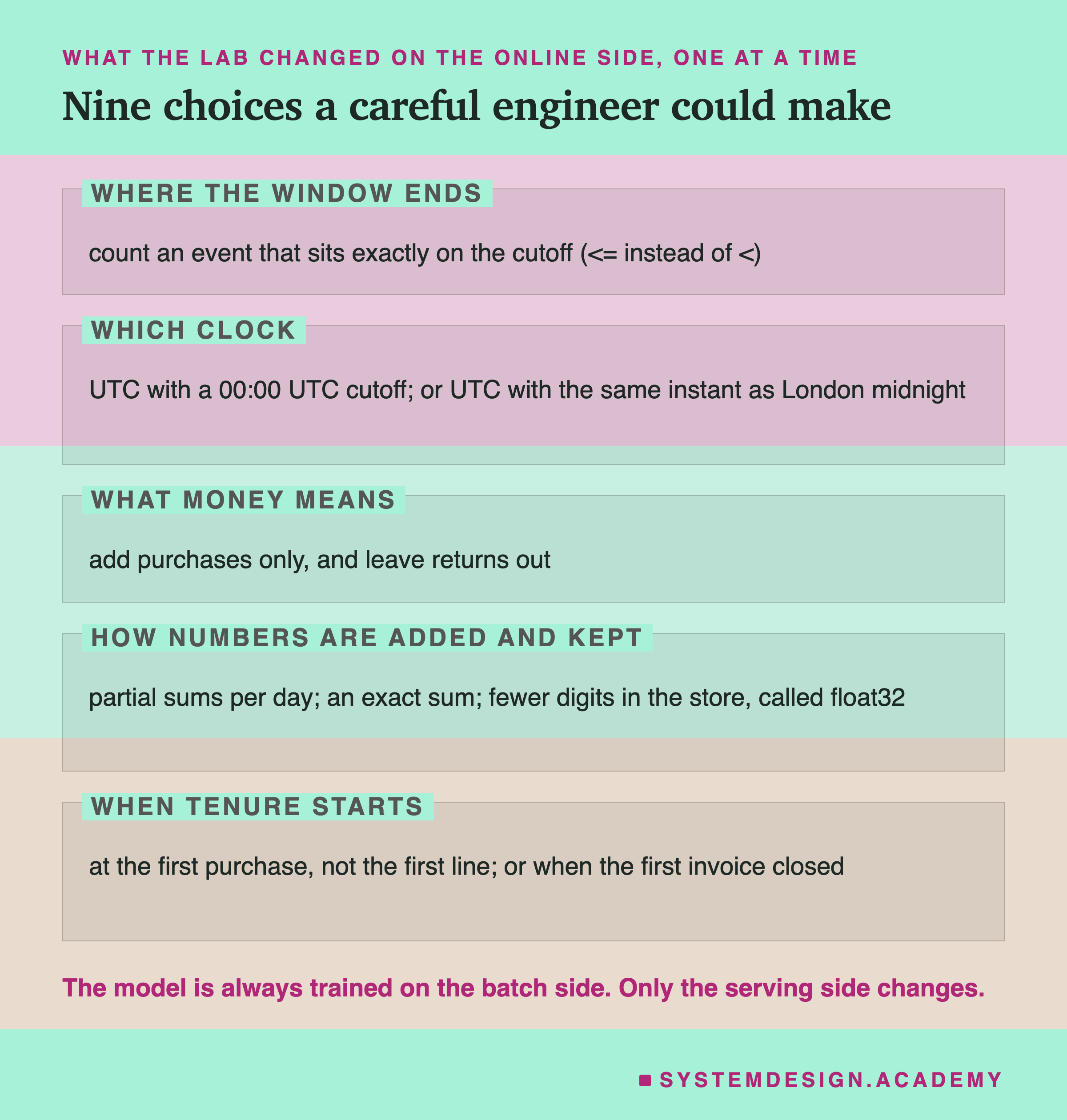
Step 1. The online side with every choice made the same way as batch, compared with batch at all 21 cutoffs, column by column.

Step 2. Nine choices, one at a time. Each is something a careful engineer could pick on purpose. None is a bug. They are grouped in the figure, and each one gets its own slide later.

Step 3. The score. The model is lesson 1's: scikit-learn's HistGradientBoostingClassifier with default settings, trained on the batch side's training rows. It then scores the test rows twice, once with batch features and once with the online ones. The batch score had to equal lesson 1's 0.5450 exactly, or the lab would stop. It did. Everything is averaged per test month, then over the five months, the same way in every lesson of this chapter.

Step 4. A parity test, the check a team would run in CI. CI, short for continuous integration, is the set of automatic checks that runs every time someone changes the code.

I also wrote down guesses before the run. Several were right. Three were not, and I name each one where the lesson comes back to it. They were about the two other ways of adding money, the returns choice, and bin edges, where I was only half right.

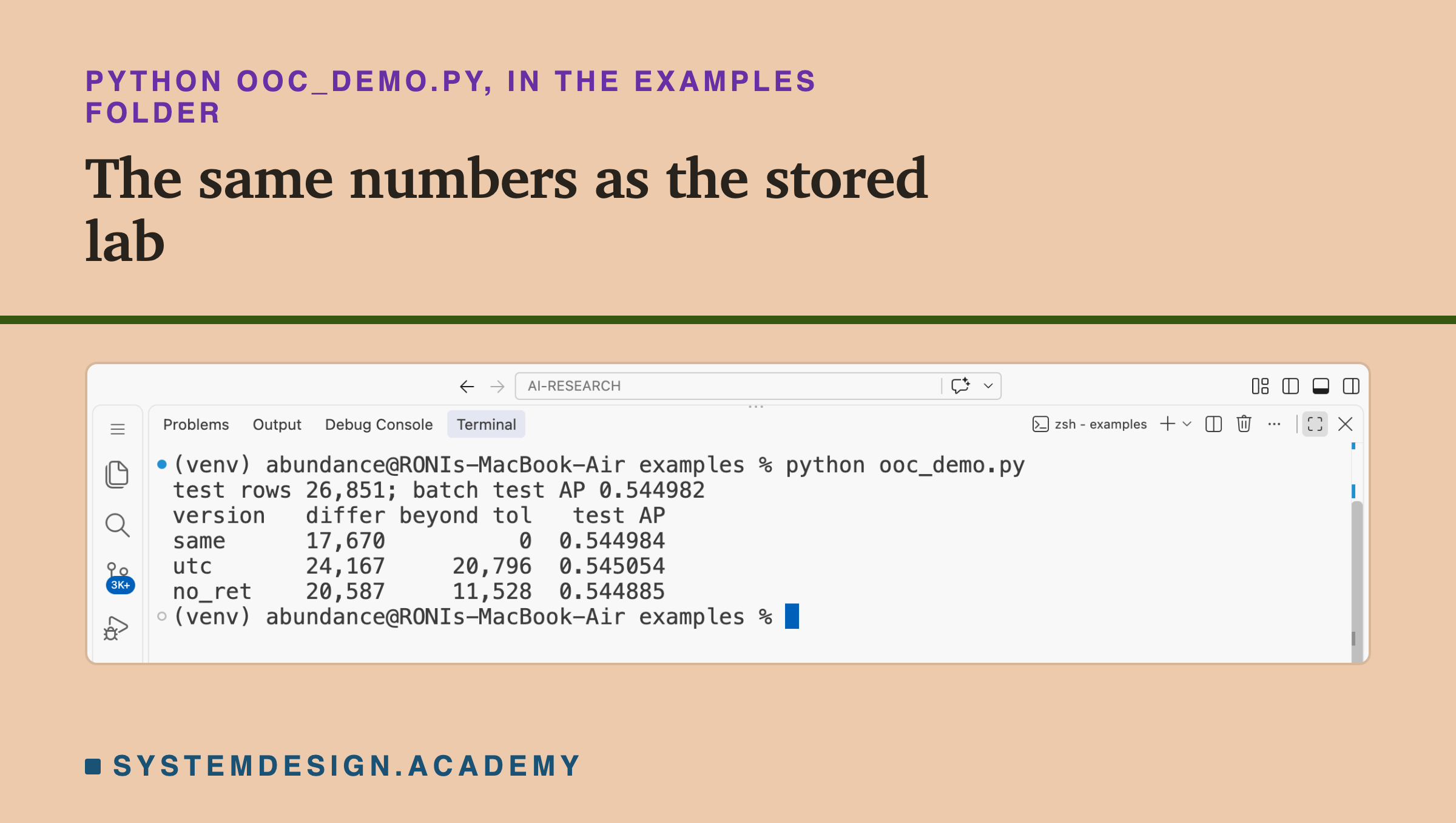
This is a real recording of the report script, ooc_report.py, on the laptop where the lab ran. It trains one model again, but mostly it reads the stored results and checks every number this lesson uses.

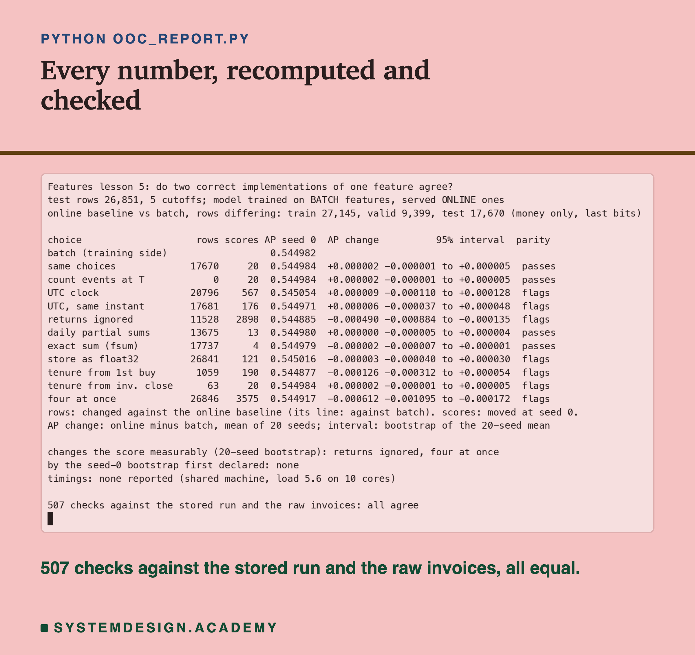
The report rebuilds both feature tables from the raw invoices and recounts every difference. Four of the counts it also predicts with plain pandas, without the loop at all. For example, the UTC clock should change recency exactly for the rows whose customer was last seen in summer time. It counted those rows directly: 19,077, the same as the loop. Then it trains the seed-0 model again and checks every score. It also checks that the demo and the playground print what they should, and that every number in this lesson appears in the lesson text. If anything disagrees, it stops with an error.

First, step 1: both sides make every choice the same way. Do they agree?

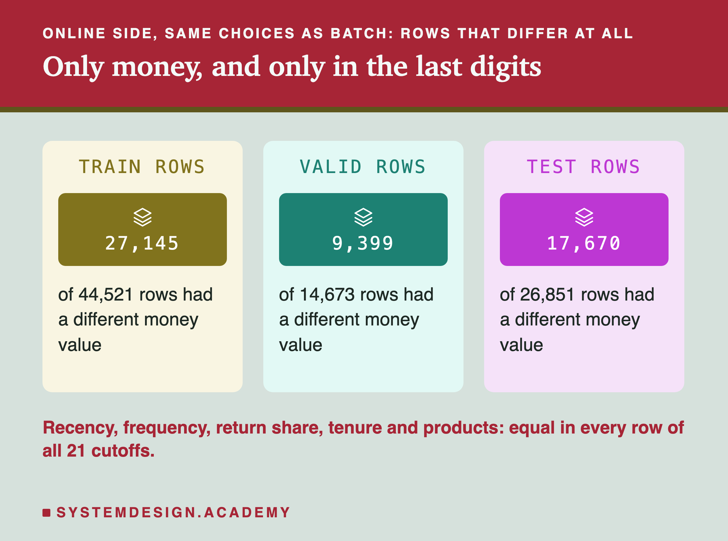
Five of the six features agreed in every row, at every cutoff. Money did not: on the test months it differed in 17,670 of 26,851 rows, which is 65.8 percent. The largest difference in any row was 1.92e-09 pounds. That notation means 1.92 times ten to the power of minus nine. In pence it is less than a millionth of a penny, far too small to see on any receipt.

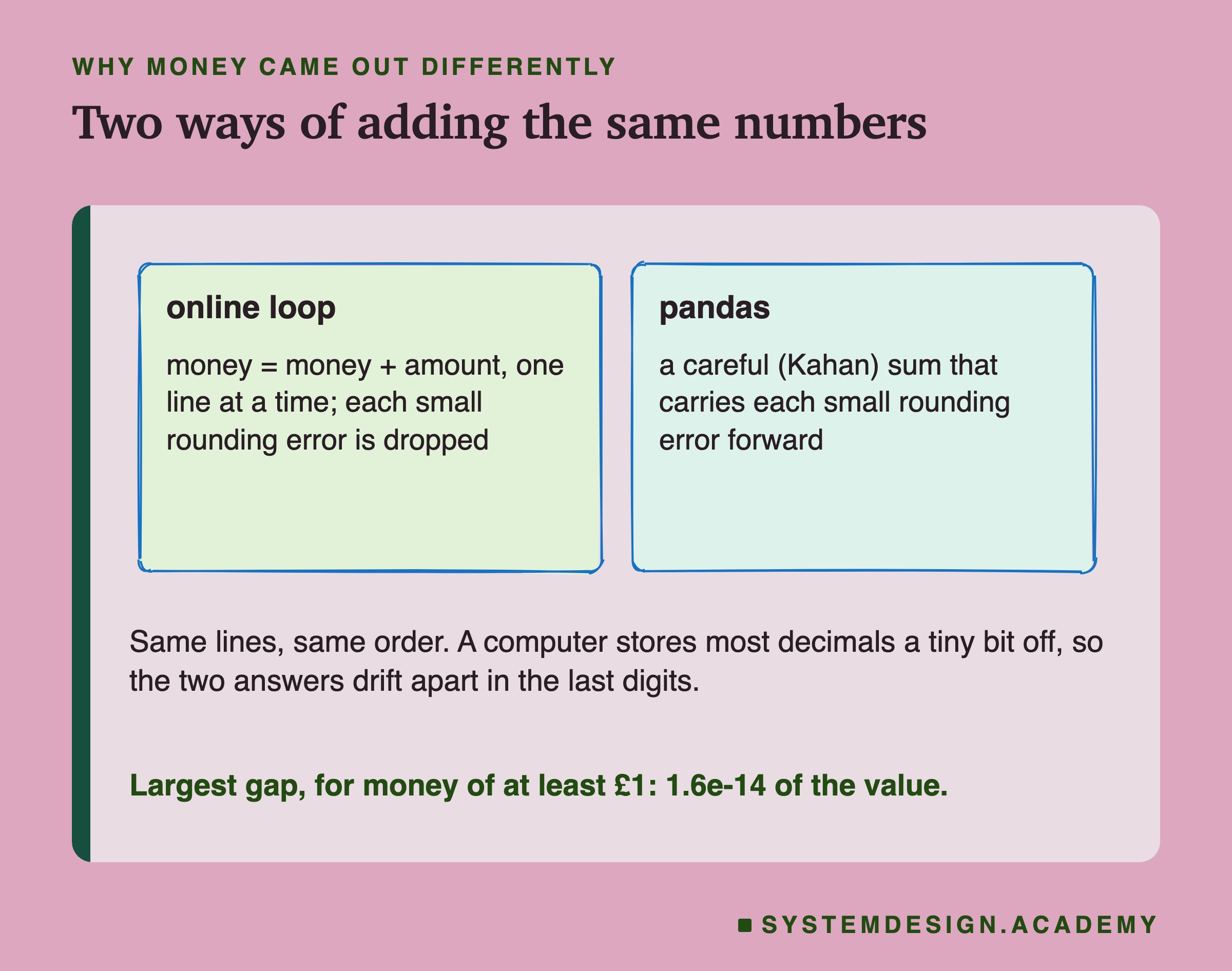
Why? Because pandas does not add numbers the simple way. Its grouped sum uses Kahan summation, a careful method that keeps track of the small rounding error at each step and feeds it back in. I checked this in the pandas source code. My loop uses a plain +=, which drops that error each time. Both are correct ways to add. They give answers that differ in the last few digits. For money of at least one pound, the biggest difference was 1.6e-14 of the value.

So "the same choices" is not enough to get the same bits. And on the very next slide that matters, because a test that demands exact equality will fail here.

Now step 2. Each choice changes one thing on the online side. I compare each one with the online side that made the same choices, so the money noise from the last slide does not count against every choice.

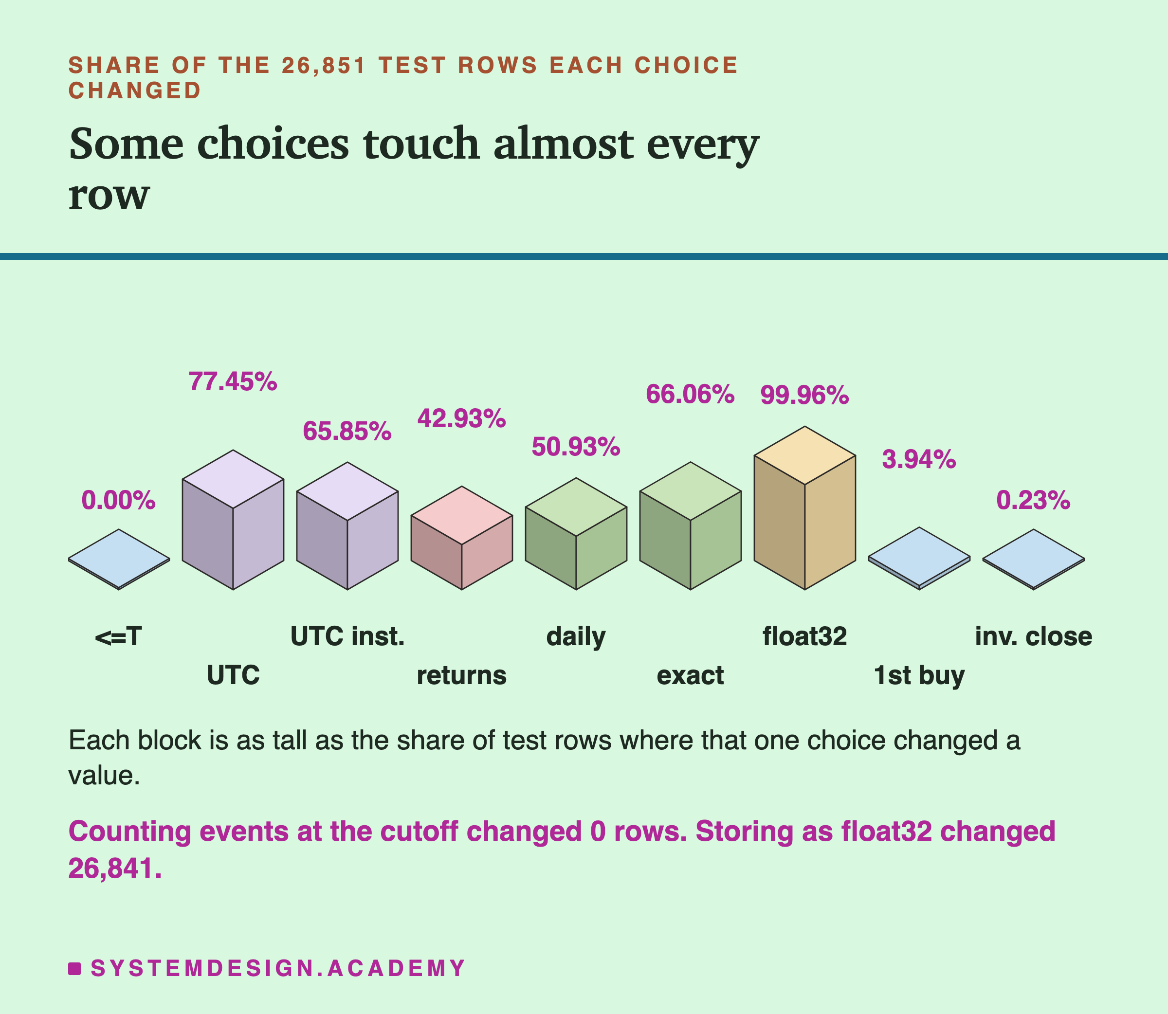
The choices touch very different numbers of rows. Counting an event that sits exactly on the cutoff changed 0 rows, because no line in this shop sits at midnight. Storing every number with fewer digits, a choice called float32 that a later slide explains, changed 26,841 rows, almost all of them, by tiny amounts. The UTC clock changed 20,796.

Rows changed is one question. The score is another.

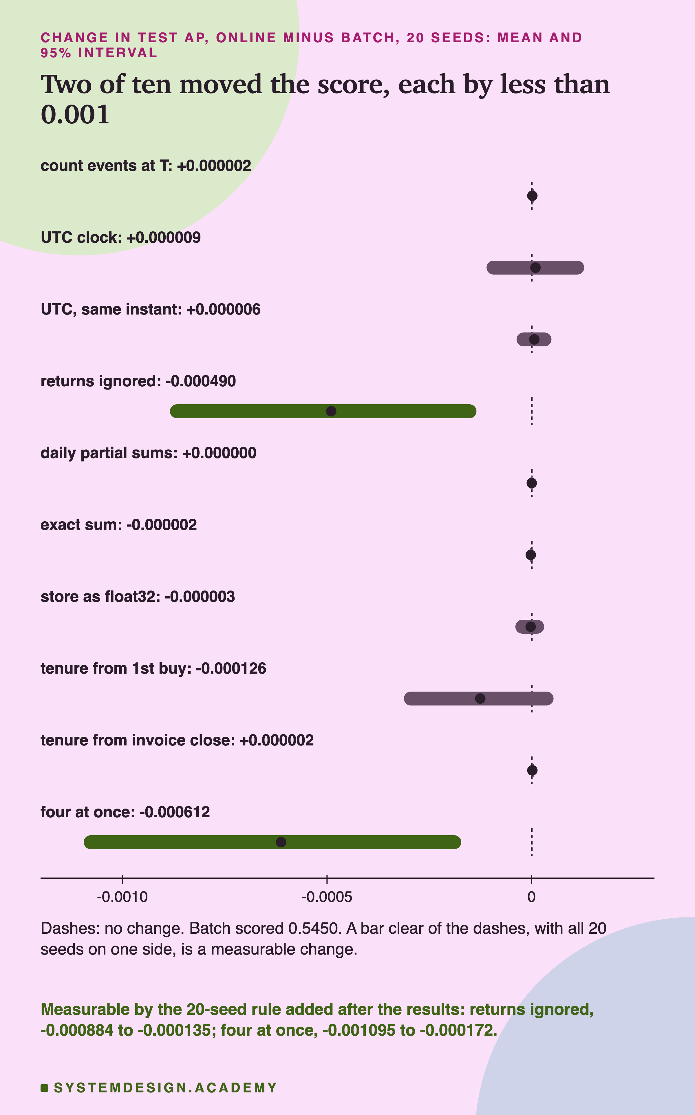
Here is the headline. The batch side scored a mean test AP of 0.544982 at seed 0, and 0.545152 averaged over 20 seeds. Of the nine single choices, only one moved the score measurably: ignoring returns in money. That verdict uses a rule I added after seeing the results, explained on the next slide; by the rule I first declared, no choice did. It lowered test AP by -0.000490 on average over 20 seeds, with an interval from -0.000884 to -0.000135. Four choices together, a post-results question on a later slide, lowered it by -0.000612.

Everything else could not be told apart from zero. And even the measurable ones are small. For comparison, lesson 1 found that better features raised AP by more than 0.15. The biggest effect here is hundreds of times smaller.

I measured two kinds of luck, as in lessons 1 to 4.

Luck in training. With more than 10,000 training rows, this model turns on early stopping by itself. Early stopping means the model stops adding trees once they no longer help on a small held-out part of the training rows. It keeps 10 percent of the training rows aside for that, chosen at random. The seed moves that choice. So I trained 20 models, seeds 0 to 19, and compared online with batch for each.

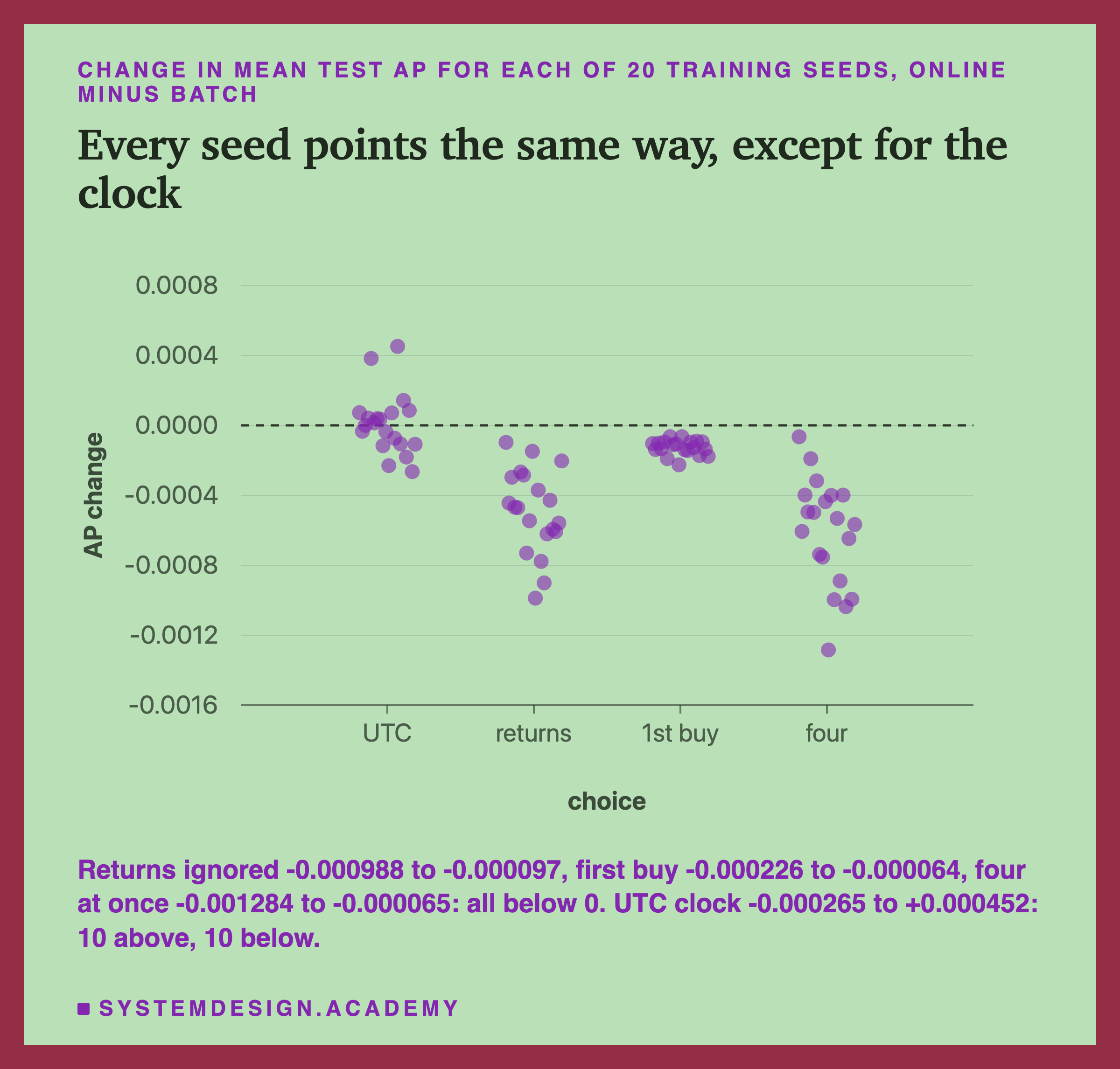
Luck in which customers were tested. A bootstrap draws the test customers again at random, with repeats allowed, 1,000 times, and works out the gap every time. The middle 95 percent of those gaps is the 95% interval.

Now the honest part. My design, written before the run, judged each choice with a bootstrap of seed 0 only. By that rule, nothing at all changed the score measurably. Then a review of the sister lessons set a rule for the whole chapter. A verdict must use both kinds of luck at once, so the bootstrap is done on the mean over 20 seeds. I added that after seeing my results, and before it ran. It changed two verdicts: returns ignored, and four choices at once.

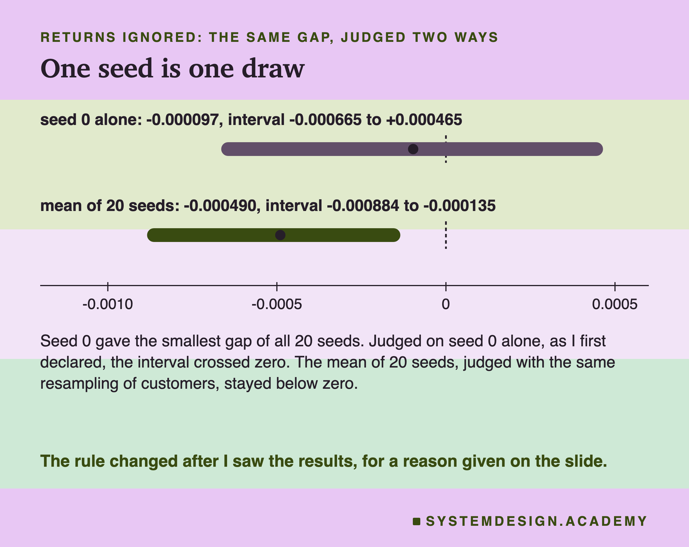
For returns ignored, seed 0 happened to give the smallest gap of all 20 seeds, -0.000097. Judged on that one seed, the interval crossed zero. Judged on 20 seeds, with all 20 below zero and an interval clear of zero, it is a real, small effect.

The same happened for four choices at once: on seed 0 its interval ran from -0.000789 to +0.000626, and on the 20-seed mean from -0.001095 to -0.000172. My guess before the run was that ignoring returns would lower the score measurably. By the rule I first declared, that guess was wrong; by the later rule, it was right.

The first clock choice: the online service keeps all time in UTC, which is common for servers. It converts each event from London time to UTC correctly, and its cutoff is midnight UTC on the 1st of the month. In summer that cutoff is 01:00 London time, an hour later than batch's. The shop has no sales between midnight and 1am, so no event moves across it.

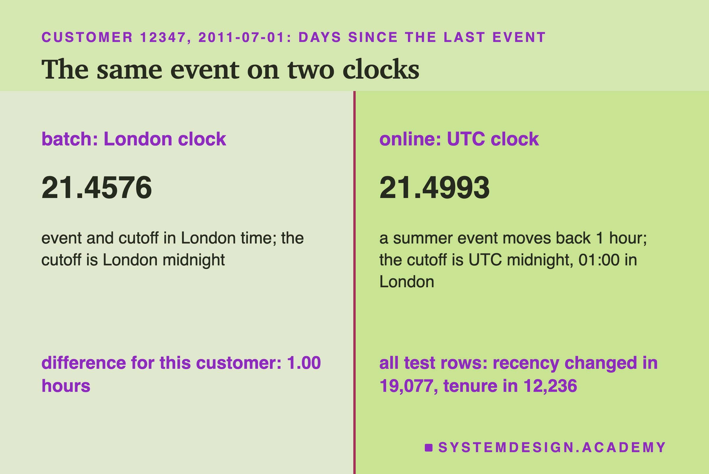
In summer, a London event at 14:00 is 13:00 UTC. The cutoff stays at 00:00 either way. So any customer last seen in summer looks one hour older to the online side. Customer 12347's recency went from 21.4576 days to 21.4993 days. Recency changed in 19,077 test rows, tenure in 12,236, and 20,796 rows had at least one change.

The second clock choice keeps UTC but sets the cutoff to the same moment as London midnight. Then the two sides differ only when the event and the cutoff are on different sides of a clock change. The online side measures real elapsed time, and the batch side subtracts wall-clock times. A wall-clock time is what a clock on the wall shows, and it jumps by an hour when the clocks change. That changed 17,681 rows.

And the score? The UTC clock moved 567 scores at seed 0. But over 20 seeds the change was +0.000009, ten seeds up and ten down, with an interval from -0.000110 to +0.000128. It cannot be told apart from zero. One possible reason, which I did not test: recency here is counted in days, and one hour is a small step on that scale. So few customers cross a point where the model's answer changes.

Stream processors have their own rules about this. Apache Flink's documentation says its hourly windows line up with the epoch, the start of computer time in UTC. To use another time zone, you add an offset "to adjust windows to timezones other than UTC-0". So the clock choice is a real one, made in real tools.

The definition said "money is the customer's spend". Batch subtracts returns, so it is net spend. A second engineer could fairly read "spend" as purchases only, and leave returns out.

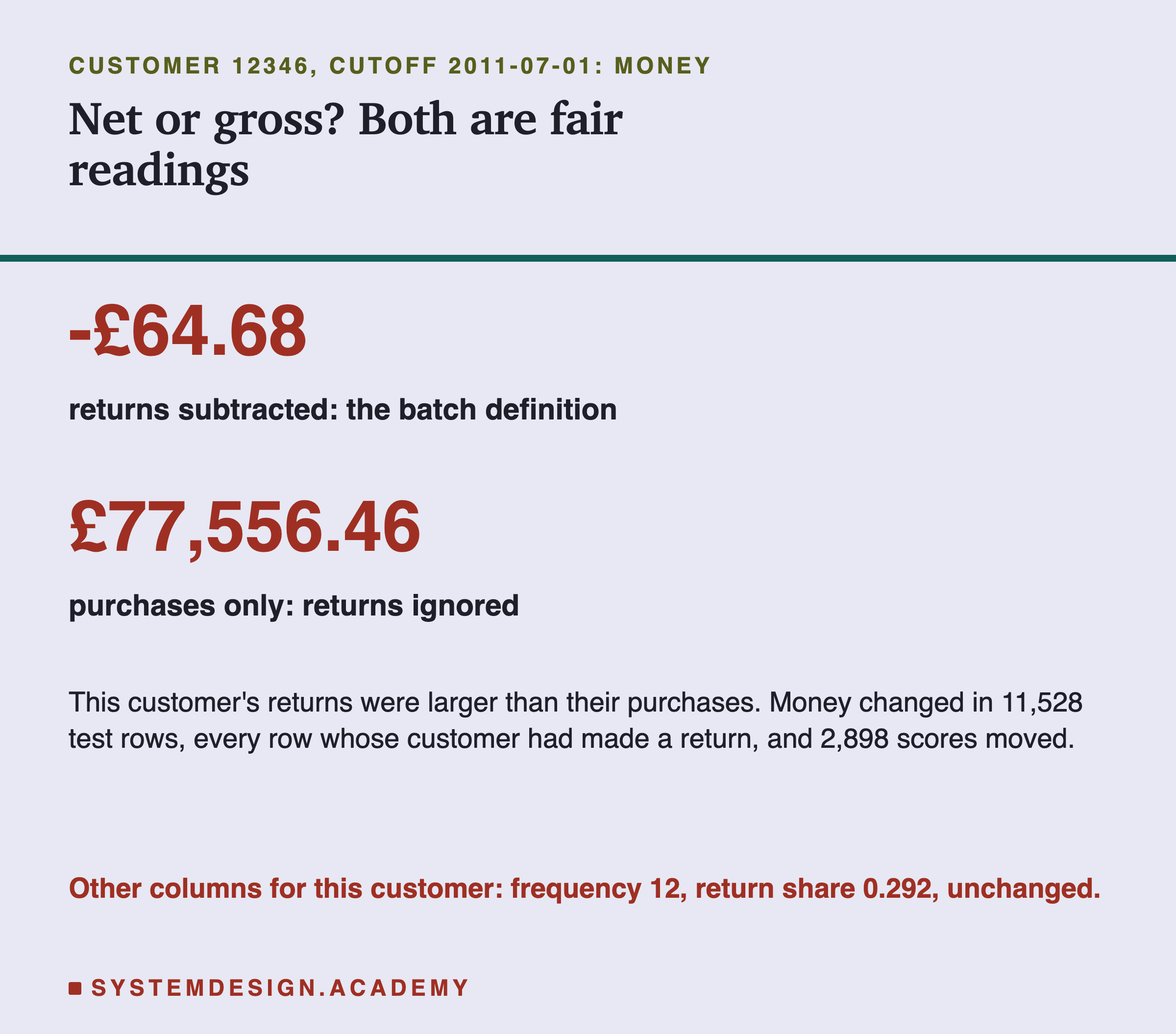
Customer 12346 shows how far apart the two readings can be. Net, they spent minus £64.68: their returns were larger than their purchases. Gross, they spent £77,556.46. Same customer, same events, two honest numbers.

This choice changed money in 11,528 test rows: exactly the rows whose customer had made at least one return. The report counted those rows separately and they match. It moved 2,898 scores at seed 0, more than any other single choice.

And it was the only single choice that moved test AP measurably: -0.000490 over 20 seeds. That fits a simple picture. Ignoring returns changes what the feature means, not just how it is rounded or which clock it reads. Tenure from the first purchase is also a change of meaning. Both meaning changes pushed every one of the 20 seeds down; only returns cleared the bar. The clock and storage choices did not. The model learned that a customer with high net spend tends to come back. The online side now shows it a number that is gross spend, which is systematically larger for anyone who returns things.

A later lesson in this chapter changes a feature's definition on purpose. Here the point is smaller: two readings of one sentence, each correct, chosen by two people who never talked.

Five choices changed rows but moved the score by an amount I cannot tell apart from zero.

Counting events at the cutoff (<= instead of <) changed 0 rows. That is true only because this shop sells nothing at midnight. On data with events at exactly the cutoff, the same choice would let an event from the prediction moment into the feature. Do not read "harmless" as a general law; read "harmless here, for a reason I can name".

Daily partial sums and an exact sum both change how money is added. The exact sum uses Python's math.fsum, which its documentation describes as "an accurate floating-point sum" that tracks "multiple intermediate partial sums". Both changed the last digits of money in more than 13,000 rows, and moved at most 13 scores at seed 0. Over 20 seeds their effect was +0.000000 and -0.000002. Before the run I guessed that these two would move no score at all. That guess was wrong: they moved 13 and 4 scores at seed 0, through the bin edges explained on the next slide.

Storing every number as float32, a 32-bit floating-point number with about seven digits of precision instead of about sixteen, changed 26,841 rows. A feature store may let you declare a column that way: Feast's schemas, for example, have both Float32 and Float64 types. Over 20 seeds the effect was -0.000003.

Tenure from the first purchase instead of the first line changed 1,059 rows, the customers whose first line was a return and who had bought since. Customer 12349 is one: his tenure went from 573.47 days to 427.44. All 20 seeds moved down, by -0.000126 on average, but the interval crossed zero.

Tenure from when the first invoice closed changed only 63 rows, by one or two minutes.

Here is something I did not expect. With every choice made the same way, the online side moved 20 scores at seed 0. The only difference was money, in the last digits. How can a difference that small change anything?

This part was added after I saw the results, and the design says so.

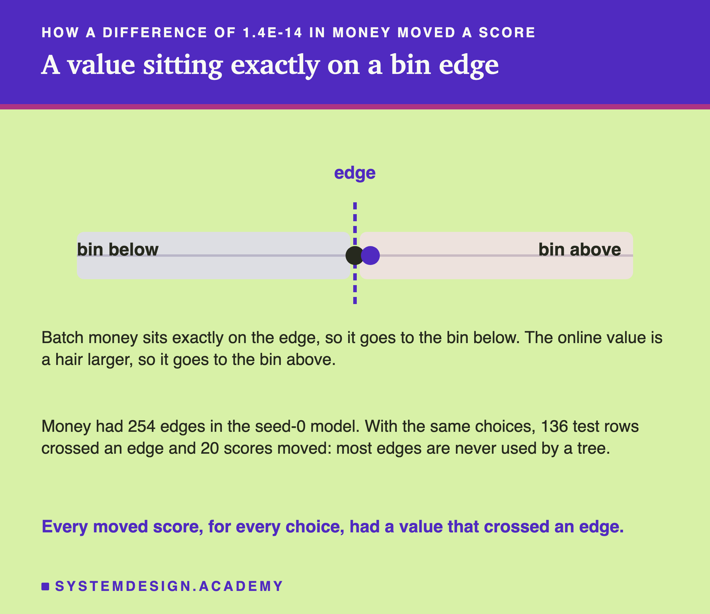
Before training, this model sorts every number into at most 255 groups called bins. The scikit-learn documentation says each feature "is binned into integer-valued bins". The cut points between bins are the bin edges. Money had 254 of them in the seed-0 model. The trees never see the exact money value, only which bin it fell into.

Some edges sit exactly on a value that real customers have. A customer whose money equals an edge goes to the bin below. Add a tiny amount to that value, and it goes to the bin above. Here the money differences that moved a score ran from 1.4e-14 to 6.8e-13. For all 20 moved scores, money sat exactly on an edge. With the same choices, 136 test rows crossed an edge, and only 20 scores moved, because most edges are never used by any tree to make a decision.

I predicted, before this part ran, that "crossed an edge" and "score moved" would be the same rows. Half right. Every moved score, for every choice, had a value that crossed an edge. But many crossings moved nothing.

AP averages over thousands of customers. A change that is small on average can still be large for one person.

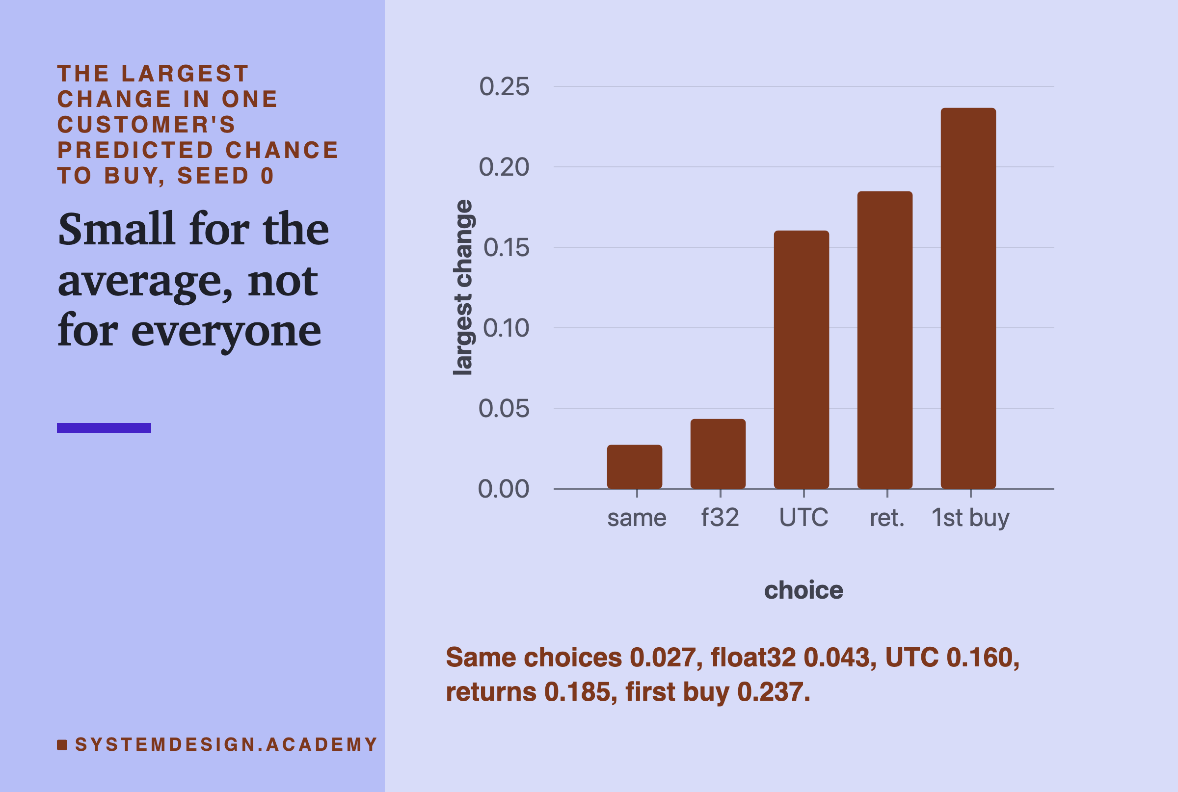
The report measured, for each choice, the largest change in any one customer's predicted chance to buy. The lab did not store this; the report computed it from the retrained seed-0 model. With every choice the same, one customer's score moved by 0.0273: the last-digit noise in money, landing on an edge. With tenure from the first purchase, one customer's score moved by 0.2366, on a scale that only runs from 0 to 1.

Why does this matter? If a team uses the score to decide who gets a coupon, the average AP is not what a customer feels. A customer near the decision line can be in on Monday's batch run and out on Tuesday's live call, with no code change at all. For a ranking measured over everyone, the effects here were small. For a decision about one person, they need not be.

A real online service would not differ from batch in just one way. So after the main results I asked one more question: what if the service keeps time in UTC, ignores returns, stores 32-bit numbers and starts tenure at the first purchase, all together? This was added after the results, and is labelled so in the lab.

Together they changed 26,846 of the 26,851 test rows and moved 3,575 scores at seed 0. Over 20 seeds, test AP fell by -0.000612, all 20 seeds below zero, with an interval from -0.001095 to -0.000172. So it is measurable, and still small. The largest change for one customer was 0.2395.

Most of that comes from returns alone, -0.000490. The other three added a little. I did not test which pairs interact.

So what should a team check? A parity test runs both sides on the same rows and compares them, column by column. The hard part is the tolerance.

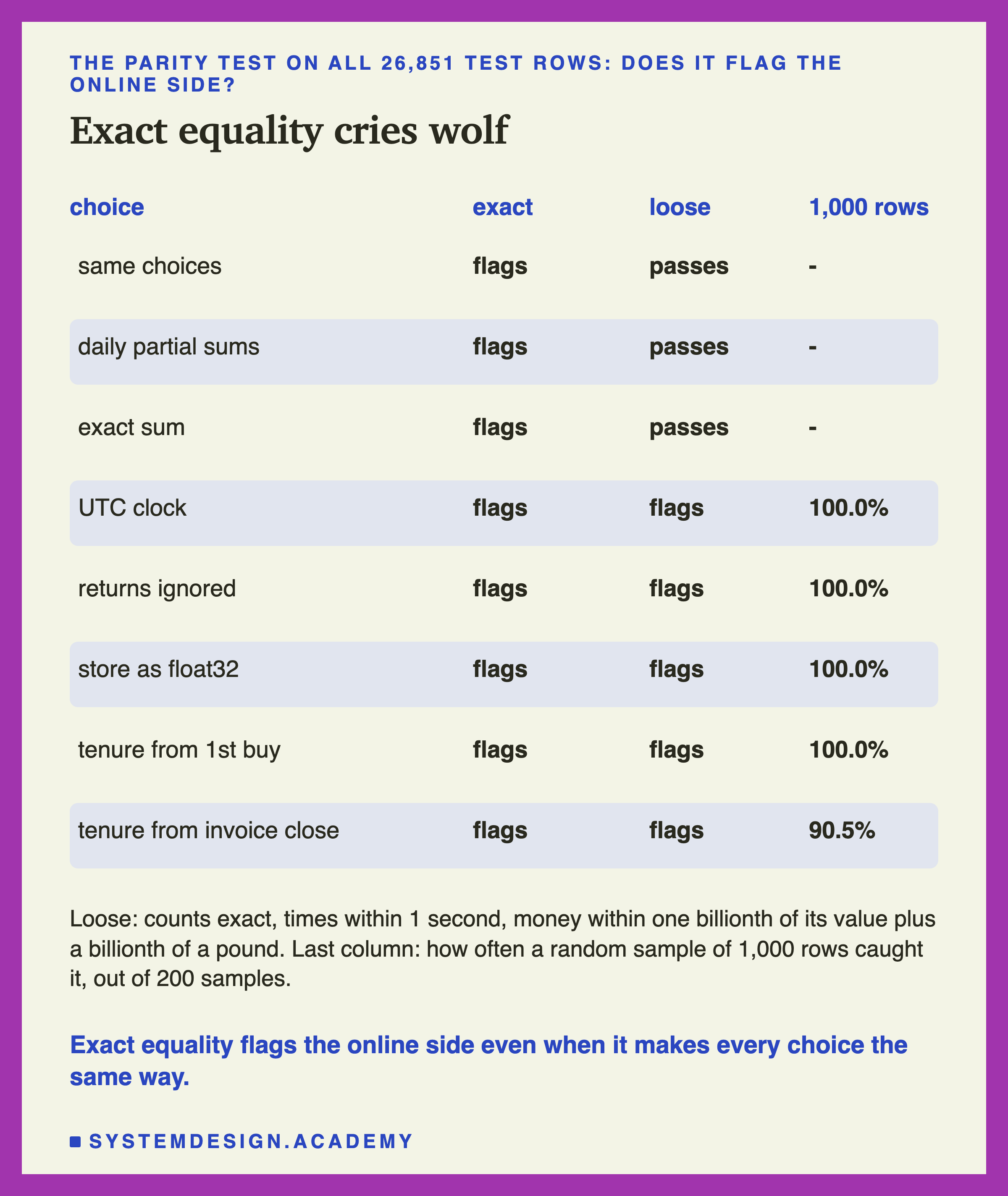
Exact equality flags every version, including the one that made every choice the same way. A test that always fails gets ignored, so it protects nothing. The figure's title calls this crying wolf: an alarm that rings so often that people stop listening.

The loose tolerance is per column. Counts, like frequency and products, must be exactly equal: there is no rounding in a count. Times must agree within one second. Money must agree within one billionth of its value, plus a billionth of a pound, so a total of exactly zero still passes. That second part matters: some customers' net money is exactly 0.0 on the batch side, and about 1.4e-14 on the online side. Why one billionth? The adding-order noise was at most 1.6e-14 of the value, so a billionth leaves a wide safety margin, and every real choice in this lab differed by far more. The loose test passed the three versions whose only difference was how money was added. It flagged the clock, the returns, float32 and both tenure choices.

Notice that the loose test also flags float32 and both clocks, which did not move the score measurably. That is fine. A parity test tells you that the two sides differ and by how much. Only the score tells you whether the difference matters. Two separate questions.

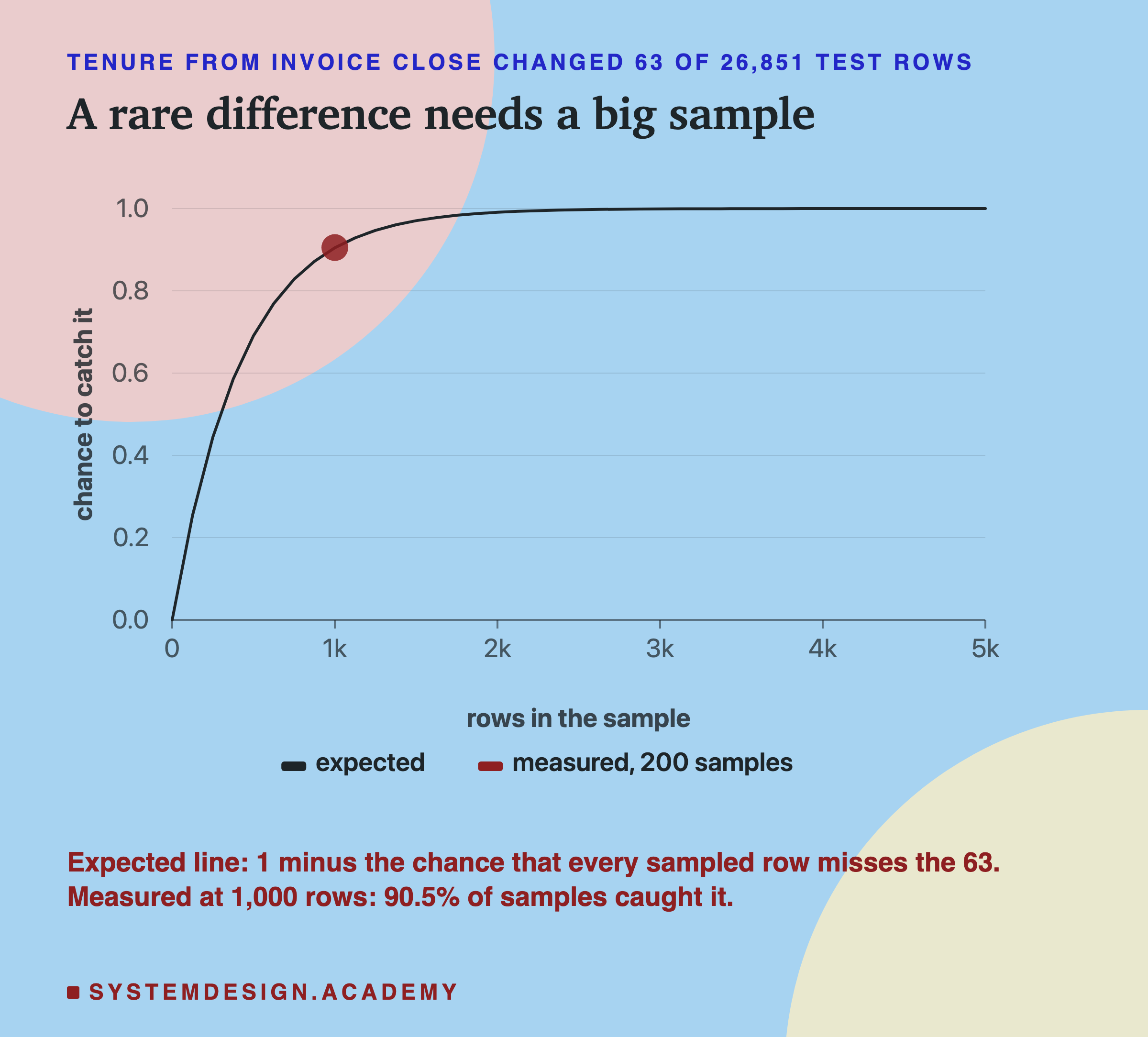
Sample size matters too. The invoice-close choice changed only 63 rows. A sample of 1,000 random rows caught it in 90.5 percent of 200 tries. So a CI check on a small sample will sometimes miss a rare difference. Run it on more rows, or on all of them at night.

The choices in this lab are not invented. Real tools make them, each one in its own documented way.

Apache Flink's documentation says a window has "a start timestamp (inclusive) and an end timestamp (exclusive)". Kafka Streams says its tumbling and hopping windows have "the lower interval bound being inclusive and the upper bound being exclusive", but that for sliding windows the bounds "are both inclusive". So two stream tools do not even agree with each other on every kind of window.

pandas adds grouped floats with Kahan summation; a plain Python loop does not. Each rule is right on its own. Mix them, one on each side of your model, and you get the kind of differences this lesson measured.

I checked each of these claims against the tool's own documentation or source code the day I wrote this lesson, and recorded the quotes in results/ooc-factcheck.json.

The full lab trains a model for every seed in each of its parts, and runs the online loop again for every choice. I wrote a small demo that does the heart of it: the batch side, one online loop with three versions, and one model.

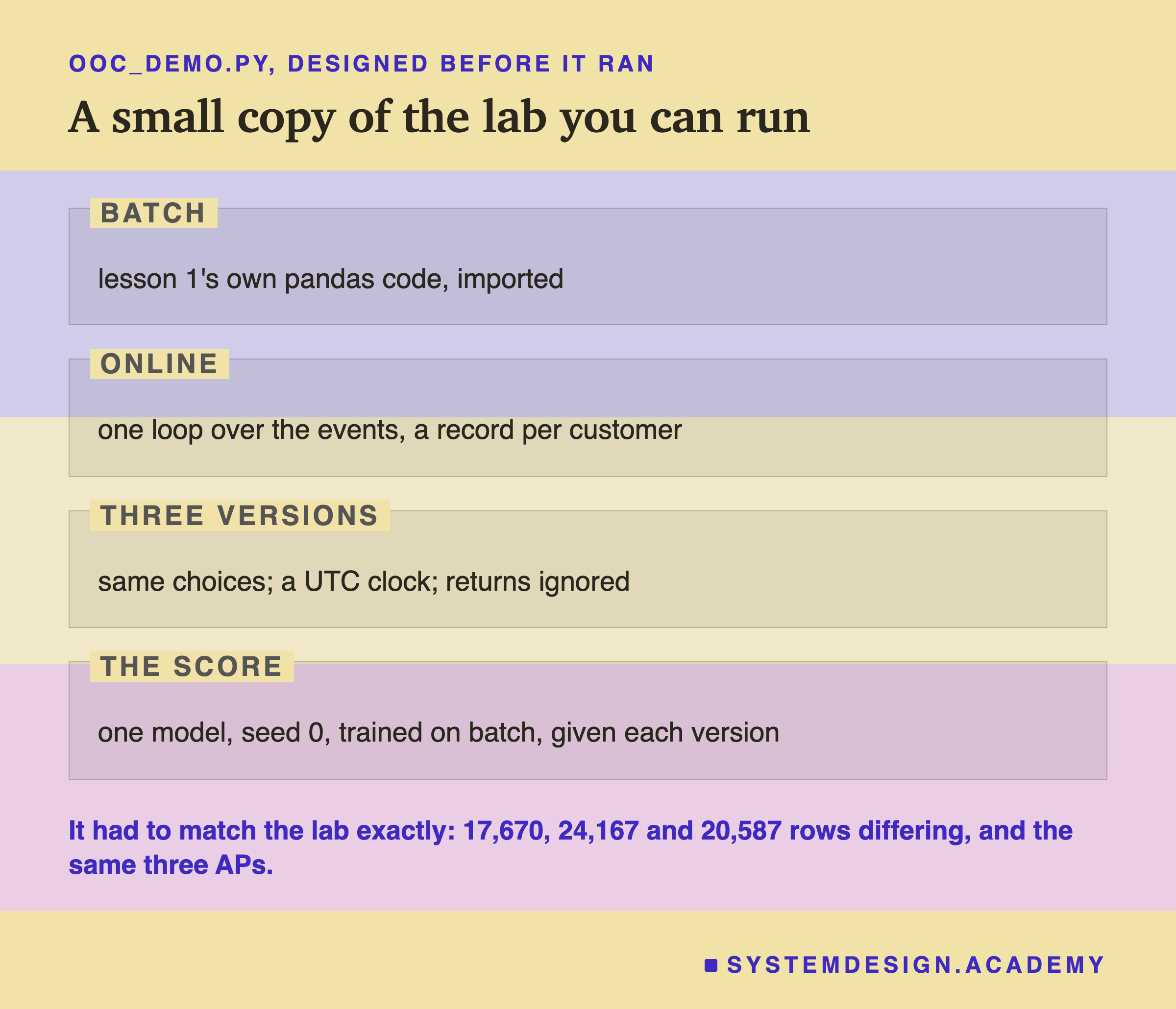
I wrote the demo's design into its docstring after the lab had run and before the demo first ran. Its loop is shorter than the lab's, written separately, so it is also a second check on the lab's loop. The rows it reports differ from batch, not from the same-choices version, so the money noise is counted in all three.

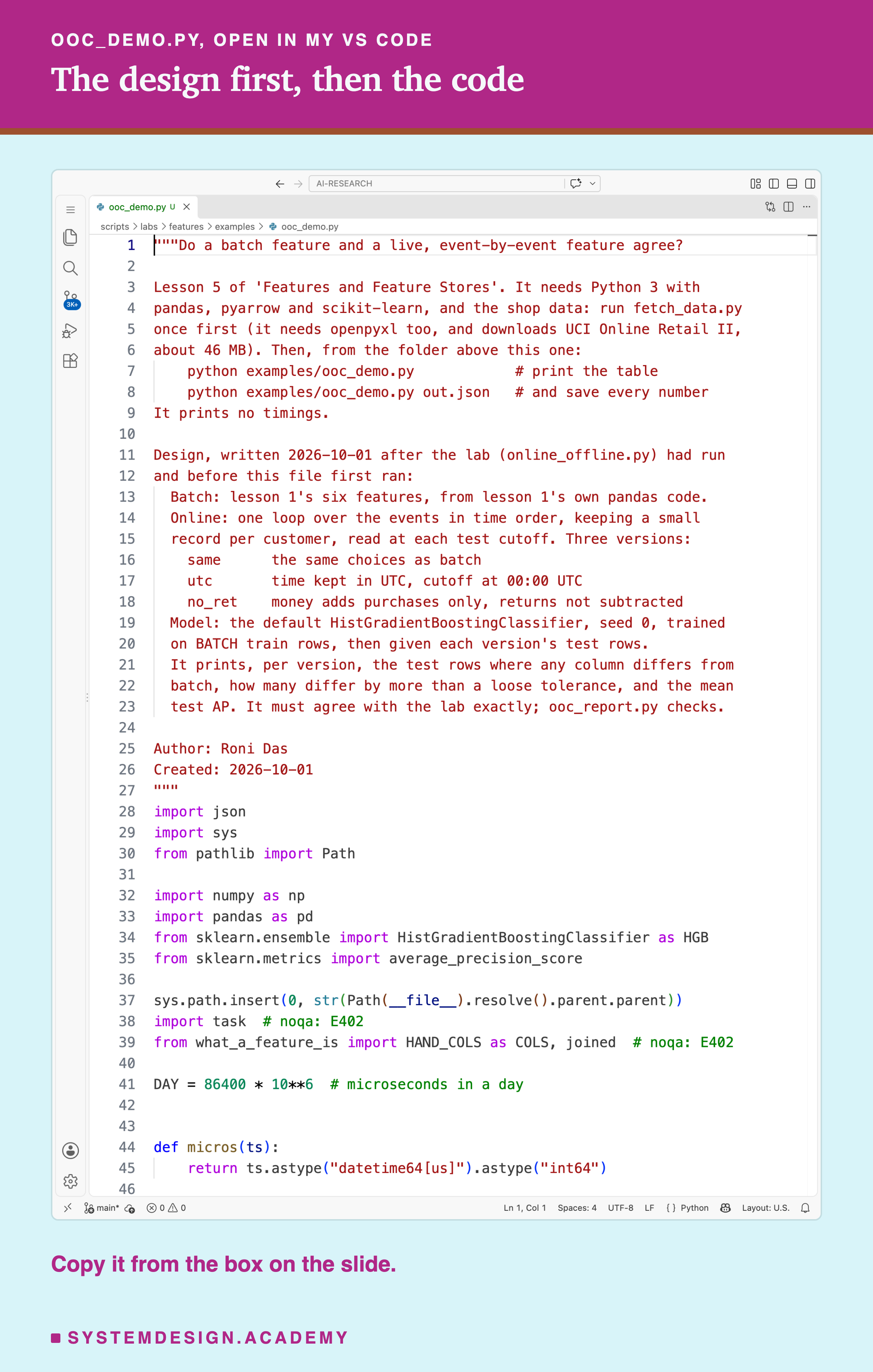
Before you run this lab. You need Python 3 with pandas, pyarrow and scikit-learn: pip install pandas pyarrow scikit-learn openpyxl. First run python fetch_data.py from the scripts/labs/features folder. It downloads the shop data once, about 46 MB, and writes one cleaned file. The demo imports lesson 1's lab file, what_a_feature_is.py, from that same folder. It needs no GPU. I ran it with scikit-learn 1.9.1 and pandas 3.0.6 on a Mac; it took well under a minute, even though other programs were using the machine at the time, so I give no exact time. These libraries run on Windows and Linux too, but I have not checked the numbers there. Give it a file name, python examples/ooc_demo.py out.json, and it also saves every number. That is how results/ooc-demo.json was made.

This box holds customer 12349's real 107 invoice lines before 1 July 2011. It needs nothing but Python, so it runs in your browser. Press Run to see the batch side and the online side side by side, column by column, and the parity test's verdict. Under that, it prints the lab's table for all 26,851 test rows.

Then change the switches at the top, one at a time. Set CLOCK = "utc" and watch recency move by an hour; tenure stays, because his first line was in winter. Set RETURNS = "ignore" and watch money rise by the returned amount. Set TENURE_FROM = "first purchase" and watch tenure drop. Set INCLUSIVE = True and see that nothing changes, because no line sits at midnight.

The report script writes this box from the raw invoices. It then runs the box with each switch flipped and checks that it prints exactly the values the lab's loop gives for this customer.

The lab is one file, scripts/labs/features/online_offline.py. It imports lesson 1's batch code instead of copying it, so the batch side is guaranteed to be the same one the model was trained on in lesson 1.

stream_inputs turns the event table into plain Python lists, the way a stream would hand events over one at a time. It also converts each London time to UTC with pandas' Europe/London zone, and stops with an error if any time falls in a clock-change hour. None does.

online is the loop. It takes a set of choices, so one function covers the same-choices version, every single choice and the four-at-once version. Each customer's record is a small dictionary. At each cutoff, snapshot reads every record into one row of six features.

align puts the online rows in the same order as the batch rows and checks that both sides have exactly the same customers at every cutoff. diff_stats counts, per column, how many rows differ at all and by how much.

flagged and loose_ok_rows are the parity test. parity_check is the version a team would put in CI: draw a sample of rows, return the columns that fail.

seedboot is the 20-seed bootstrap. It computes AP for each resample from per-row weights, and before using that fast method it checks it against scikit-learn's own on resampled rows.

Testing parity with exact equality. Here it flagged the online side that made every choice the same way. A check that always fails is soon switched off.

Testing parity on a tiny sample. A difference in 63 rows of 26,851 escaped one sample of 1,000 rows in about one try out of ten.

Assuming a parity failure means a broken model. Five of the six choices that the loose test flagged moved the score by an amount I cannot tell apart from zero. Measure the score before you panic.

Assuming a passing average means every customer is fine. One customer's chance moved by 0.2366 for one choice, and 0.2395 for four at once, while the average barely moved.

Leaving a definition in words only. "Spend" had two fair readings. Both choices that changed meaning pushed every seed down, and one of them, returns, cleared the bar. The clock and storage choices did not.

When this matters most. My guess, not tested here: when a model reacts to small input changes, like a straight-line model, which uses the exact value instead of a bin. When decisions are made per customer at a threshold. When features are about time of day, where an hour is a big step.

When it matters less. This is also my guess. It matters less when features are counted in days or larger units and the model works on bins. It also matters less when you judge it by an average over many customers, as here.

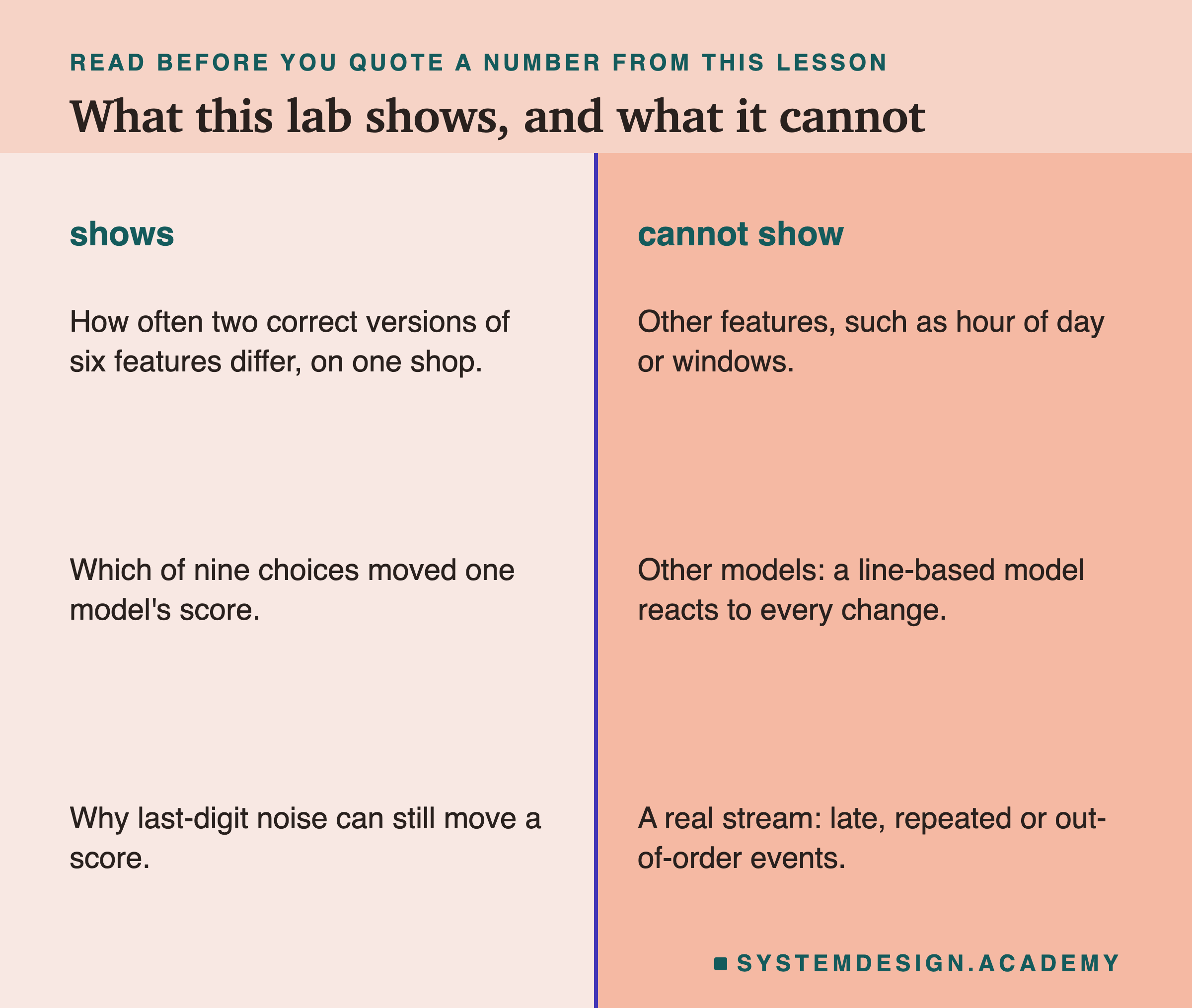
One shop, six features, one model. Recency and tenure are counted in days, and the model sorts every value into bins. Both of those soften small differences. A model that uses exact values, or features measured in hours, could react much more. I did not test either.

A clean stream. My loop reads the events in perfect time order, each exactly once. A real stream can deliver events late, twice, or out of order. The next lesson in this chapter is about late events.

Nine choices. I picked choices that a careful engineer could make on purpose. There are many more, and I tested none of the bugs, on purpose.

A rule changed after the results. The 20-seed bootstrap replaced the seed-0 bootstrap I first declared. I report both, and the change is labelled in the lab.

No timings. The machine was shared with another lab, so I report no speed numbers.

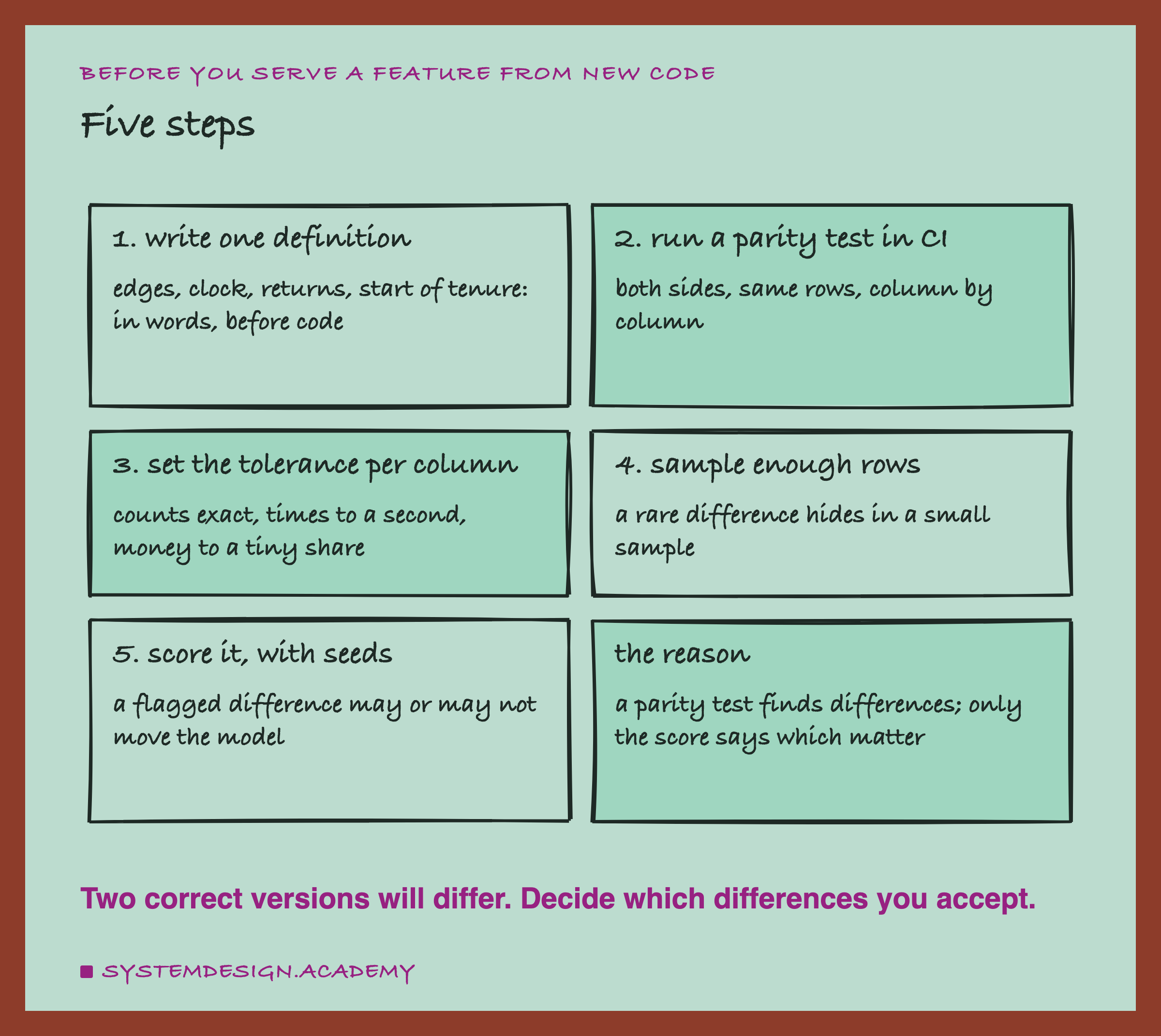
These are the steps I would take the next time a team serves a feature from new code.

1. Write one definition, with its edge cases. Here "spend" had two fair readings, and only that one moved the score.

2. Run a parity test in CI, comparing both sides on the same rows, column by column.

3. Set the tolerance per column. Exact equality failed the correct online side in 17,670 test rows.

4. Sample enough rows, or run the full comparison at night.

5. Score what the test flags, with several seeds, before you decide it matters.

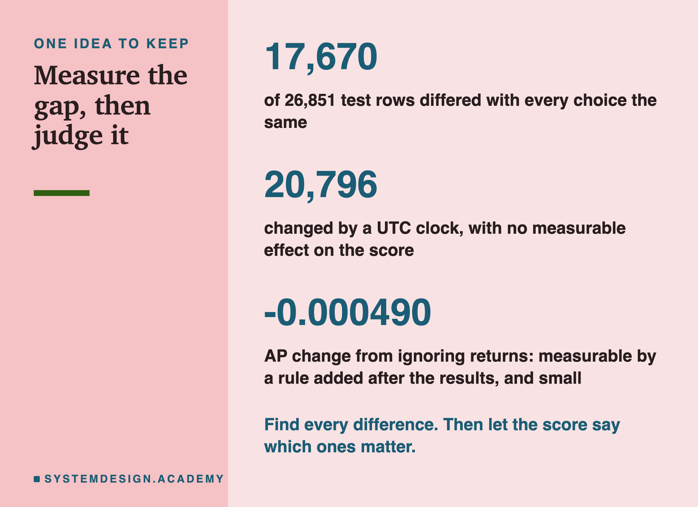
The one idea to keep: two correct implementations of one feature will not agree bit for bit. On this shop, almost none of the differences moved the score. Both changes of meaning pushed every seed down. Only ignoring returns cleared the bar, and only by a rule I added after seeing the results; by the rule I first declared, none did. The clock and storage choices did not move it. Find every difference, then let the score decide which ones you must fix.