The Letters That Come Late
Let me start with an office desk.
Imagine the front desk of a big office building. Every evening, the man at the desk writes up a tally of the day's post: how many letters came for each company in the building. Each letter has a postmark, the date it was sent. Most letters come the next morning. A few take days, because one post office was slow or one van broke down.
So every evening he has a choice. He can write up the tally now, and miss the letters that are still on their way. Or he can wait a day or two, catch most of the slow ones, and give the companies their tally later.
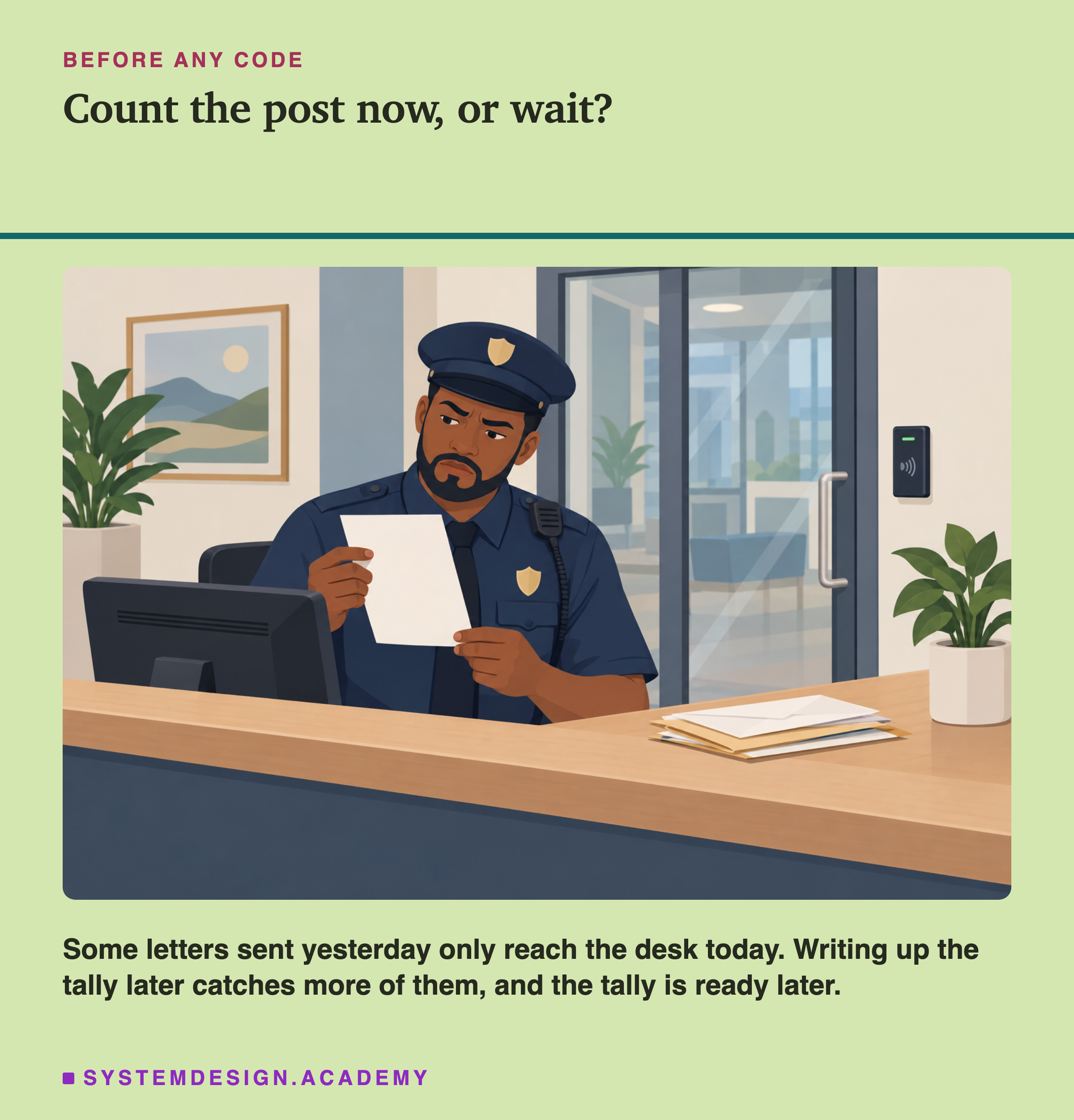
There is a second choice too. When a letter turns up after the tally is written, what does he do with it? He can add it to the next tally, or he can throw it away because its day is already closed.
A feature pipeline has exactly these two choices. This lesson measures what each one is worth, on data from a real shop, with one big warning that the next slides explain: the delays are invented.
Where This Lesson Starts
This is the sixth lesson of the chapter on features and feature stores. It uses the same shop data, the same prediction task and the same model as the lessons before it.
The first lesson, what a feature is, built six made features from each customer's history: recency, frequency, money, return share, tenure and products. With those six, the default model reached a test average precision of 0.5450. In this lesson, the model with the true features is exactly that model, checked to the last digit on all 20 seeds.
The third lesson, feature freshness, asked how old a feature can be before it costs anything. On this task, features up to two weeks old cost nothing its tests could tell apart from zero. Keep that in mind. It is the main reason the result of this lesson is small.
The data engineering chapter's first lesson, batch vs streaming data, defined event time, processing time, watermarks and allowed lateness, with sources. Its lab could not measure them, because its data had no arrival times. I do not repeat those definitions in full here. This lesson measures what they do, as far as invented delays allow.
The Words You Need First
Please read this slide slowly if any word is new. Every slide after it uses these words.
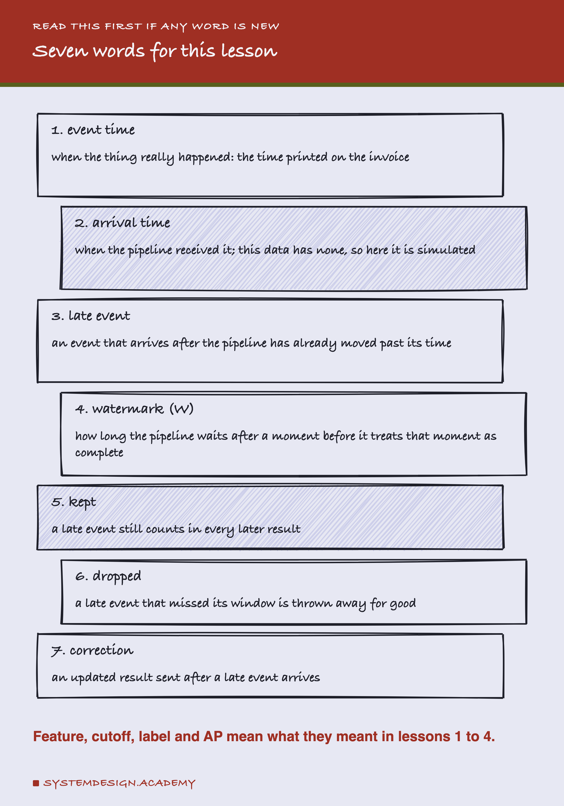
Event time. When something really happened. For an invoice, the time printed on it. Think of the postmark on a letter.
Arrival time. When the pipeline received the event. Think of the moment the letter reaches the desk. The gap between the two is the delay.
Pipeline. The program that turns raw events into features, step by step. Here it is a stream job, a program that runs all the time and handles events as they come in.
Window. A stretch of time whose events are added up together, like one day.
Watermark. How long the pipeline waits after a moment before it treats that moment as complete. I write it W. A watermark of 6 hours means: at 06:00, the pipeline treats midnight as done, and sends the result for midnight. Real engines work the watermark out from the event times they have seen, but the idea is the same.
Late event. An event that arrives after the watermark has passed its time.
Kept, dropped and correction. The three things a pipeline can do with a late event: count it in later results, throw it away, or send an updated result.
How I Score a Model, and How Sure I Am
Every result slide uses these words, so here they are once more, in short.
Average precision (AP). The model gives each customer a score. Sort the customers from highest to lowest. Walk down the list, and each time you meet a real buyer, note the share of buyers so far. AP is the average of those shares. A perfect list scores 1. A random list scores about the share of buyers, which here is about 0.2. Higher is better. I work out AP for each of the five test months on its own, then take the plain mean of the five.
Seed. A number that fixes the random choices. Here a seed fixes two things: the model's random choices in training, and the random delays the lab draws. Seed 3 of the model always goes with seed 3 of the delays. I run 20 seeds, 0 to 19, and report the mean and the spread. One seed is never a finding.
Bootstrap. A way to ask "what if the test had held slightly different customers?". Draw the test customers again at random, with repeats allowed, 1,000 times, and work out the difference each time. The middle 95 percent of those differences is the 95% interval. If it includes zero, the difference cannot be told apart from luck.
Paired. Every comparison uses the same customers, the same seed and the same redraw on both sides. So the only thing that differs is the one thing being tested.
The bootstrap in this lesson is taken over the mean of all 20 seeds, not over one seed. A later slide says why that changed while I was building the lab.
The Data Has No Arrival Times
This is the most important slide in the lesson, so I put it early.
The shop data, UCI Online Retail II, gives each invoice line one time. In the dataset's own words, it is "the day and time when a transaction was generated". It does not say when any system received the line. So this data has event times, and no arrival times at all.
To study late data, I had to invent the arrivals. For every invoice, the lab draws a random delay and adds it to the invoice's real time. All lines of one invoice share one delay. Every arrival time, every delay, and every number that depends on them in this lesson is simulated. I label them so on every figure.
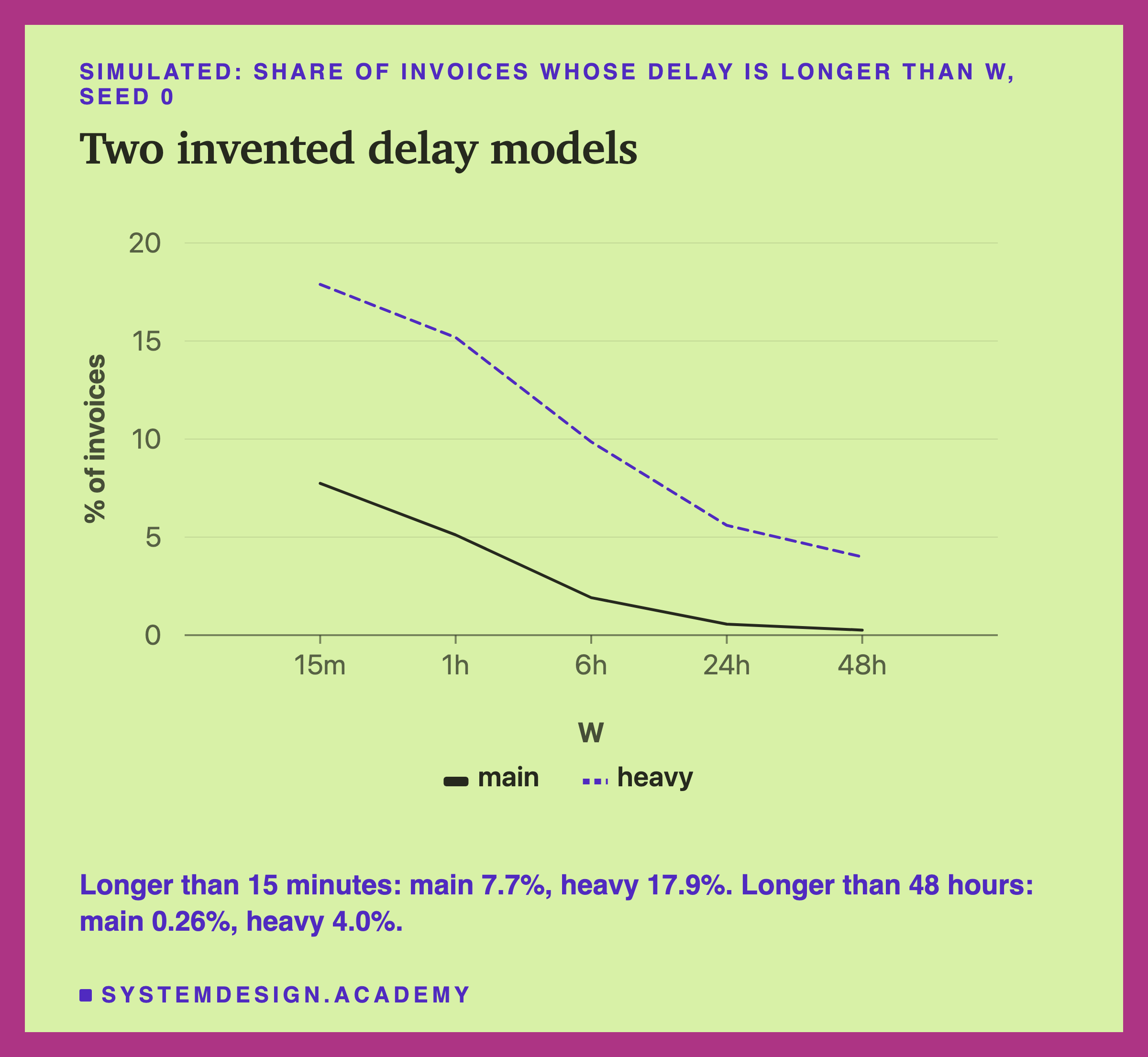
I wrote down two delay models before any draw, and did not change them:
- Main. 90 percent of invoices arrive within minutes: the delay follows an exponential curve with a mean of 2 minutes. The other 10 percent form a long tail: a lognormal curve with a middle value of 1 hour, spread wide (sigma 2.0), so some take days.
- Heavy. The check with a heavier tail. 80 percent within minutes, 20 percent with a middle value of 6 hours and a wider spread (sigma 2.5).
A lognormal curve is one where the logarithm of the value follows the familiar bell curve. It is a common shape for waiting times, because most waits are short and a few are very long. I claim nothing more about it. I do not know how late this shop's data really arrived, and nobody can learn it from this dataset.
One Real Order, Nine Hours Late
Here is one real customer at the test cutoff of 1 November 2011, with one simulated delay.
I fixed the rule for choosing them before the run. Take main delays, seed 0, the kept policy and W = 0. At the latest test cutoff that has one, take the smallest customer id among rows with a missing invoice. Only one row qualified at 1 November. So this customer was picked because their order is late. Most customers are not.
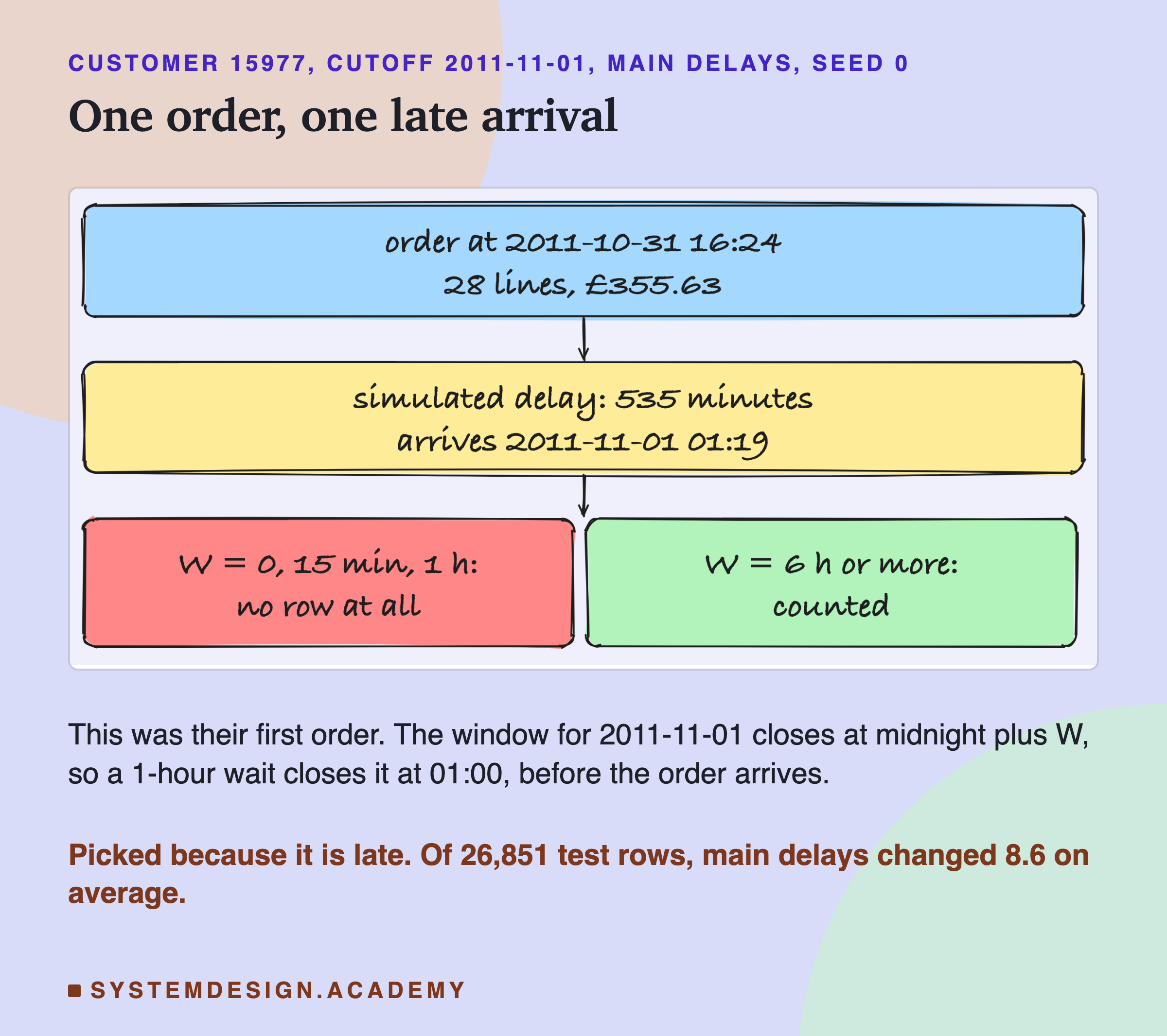
Customer 15977 placed their first ever order at 16:24 on 31 October: 28 lines, £355.63. The lab drew a delay of 535 minutes for it, about 9 hours, so it arrives at 01:19 on 1 November.
The result for 1 November is sent at midnight plus W. With W of 0, 15 minutes or 1 hour, that is before 01:19. The pipeline has never seen this customer, so it has no row for them at all. All six features are empty. With W of 6 hours or more, the order is in, and the row is right.
And this customer did buy again in November. A model that never heard of them could not rank them well.
What a Pipeline Does With a Late Event
The lab tests two policies. Each one is a different answer to the desk's second question: what to do with a letter that comes after the tally.
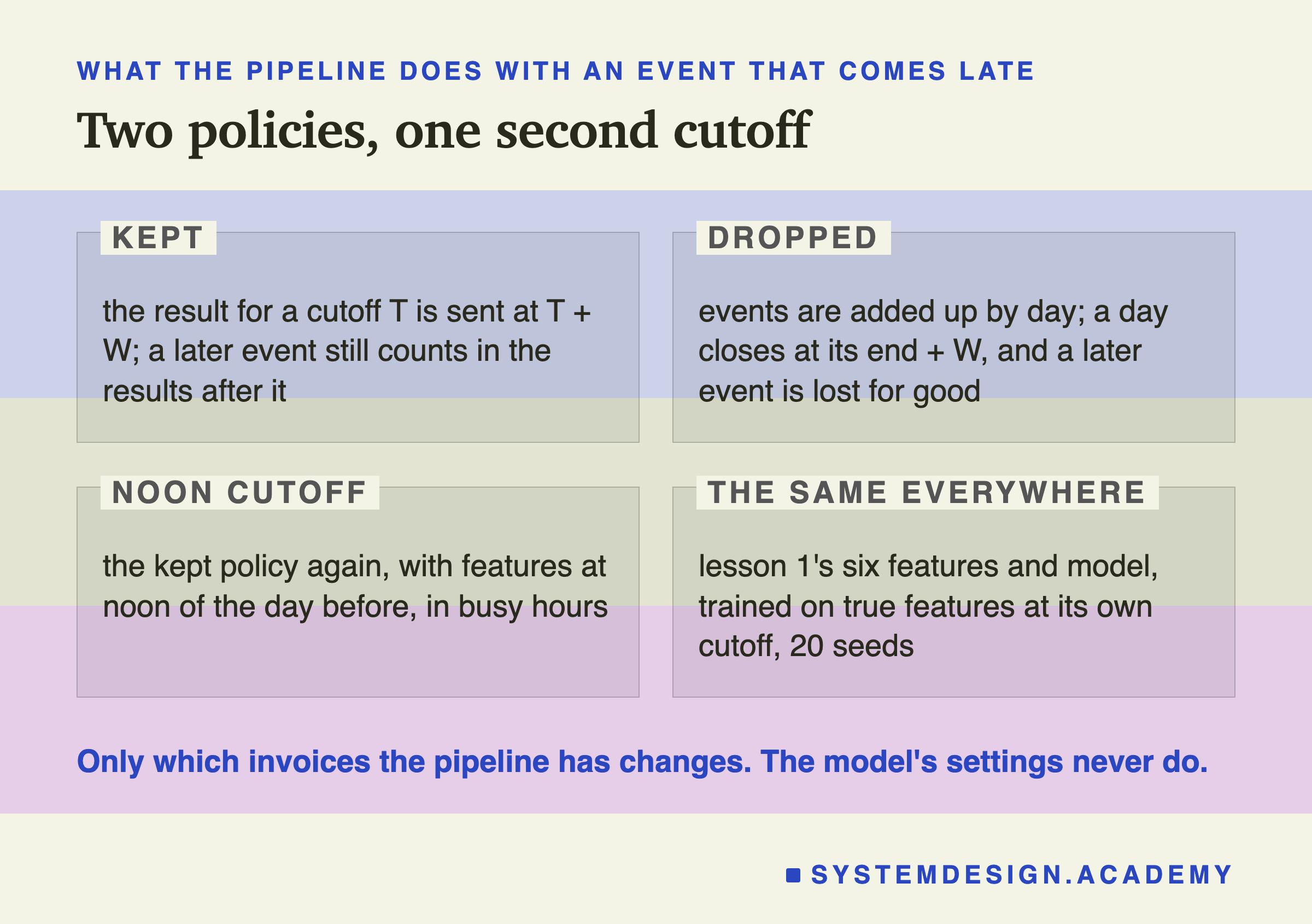
Kept. The pipeline keeps every event in its memory, which streaming engines call state. A late event misses the result that was already sent, but it counts in every result after that. So at a cutoff T, the features miss only the events still on their way at T + W. Each of those rows would need a correction later, if the pipeline sends one.
Dropped. The pipeline adds events up day by day, in daily windows. A day's window closes when the watermark passes the end of that day. An event that arrives after its own day has closed is thrown away and never counted again. So the features at T miss late events from every day in the customer's whole history, not only the last one.
The model is the same for every pipeline. It is trained on the true features, built later from the complete log of events. Only the live features it is served come from the pipeline.
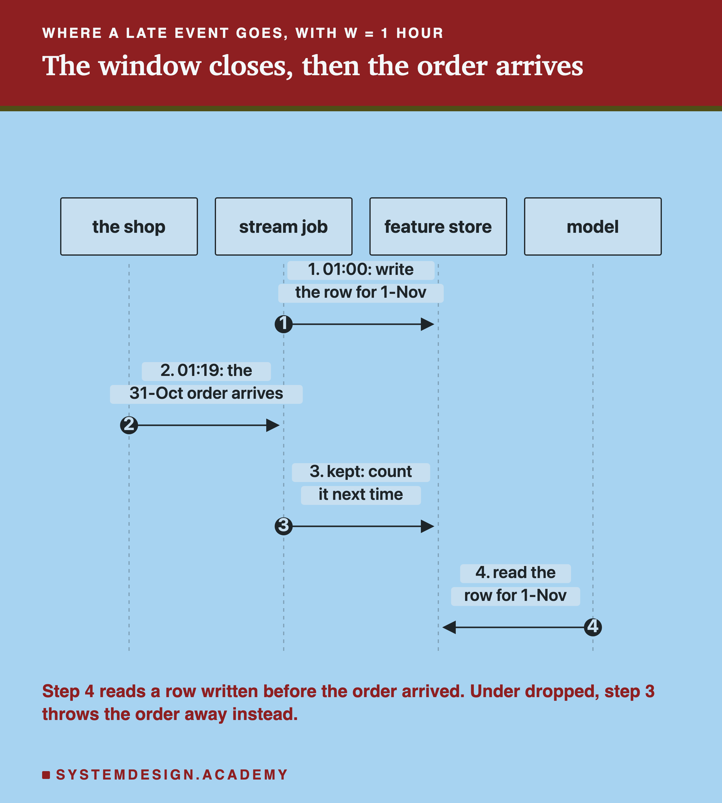
This sequence is customer 15977 again, with W of 1 hour. The features are written at 01:00. The order arrives at 01:19. Under kept, the order will count in the next result, but the row the model reads for 1 November is already written without it.
What Real Engines Do With Late Data
The two policies are not my invention. Here is what the documentation of four common stream engines says, checked on the day I wrote this lesson.
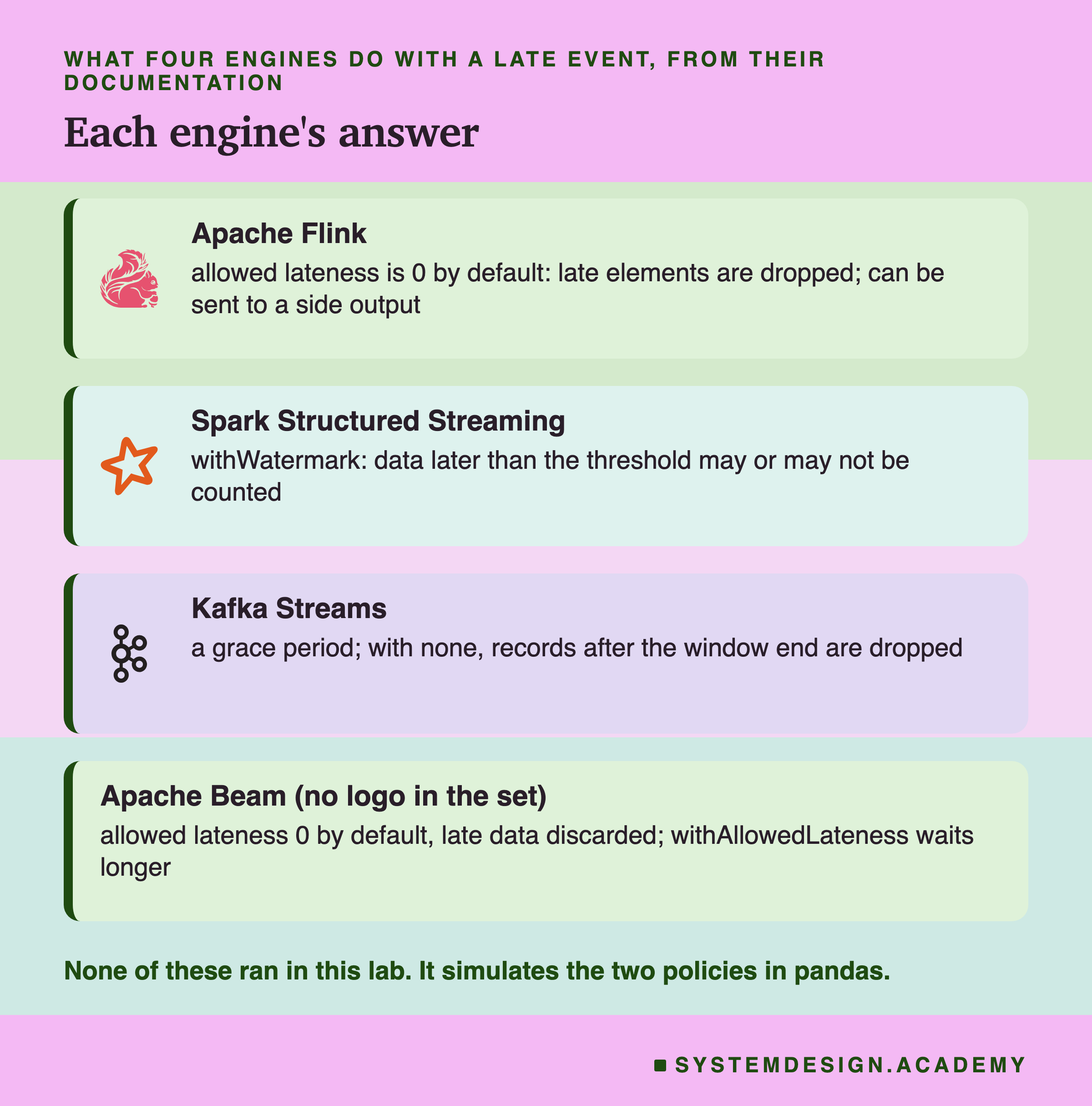
Apache Flink says: "By default, the allowed lateness is set to 0. That is, elements that arrive behind the watermark will be dropped." You can set a longer allowed lateness, and then a late element can fire the window again; Flink says those outputs "should be treated as updated results". It is the correction path from the desk story. Dropped elements can also be sent to a separate stream, which Flink calls a side output.
Spark Structured Streaming uses withWatermark. Its guide says data within the threshold is counted, and data later than it "is not guaranteed to be dropped; it may or may not get aggregated". So Spark's late data is somewhere between my two policies.
Streams, the stream library that comes with Apache Kafka, calls it a grace period. With no grace period, its documentation says "out-of-order records arriving after the window ends are considered late and will be dropped".
Apache Beam says that with its default settings "late data is discarded", because the default allowed lateness is 0, and withAllowedLateness lets you wait longer.
So my dropped policy is close to Flink's and Beam's defaults, and kept is what you get by keeping state open, at a memory cost. The lab simulates both in pandas. None of these engines ran here.
A Fact About This Shop: the Quiet Evening
Before any result, one fact about the data that changes everything at small W.
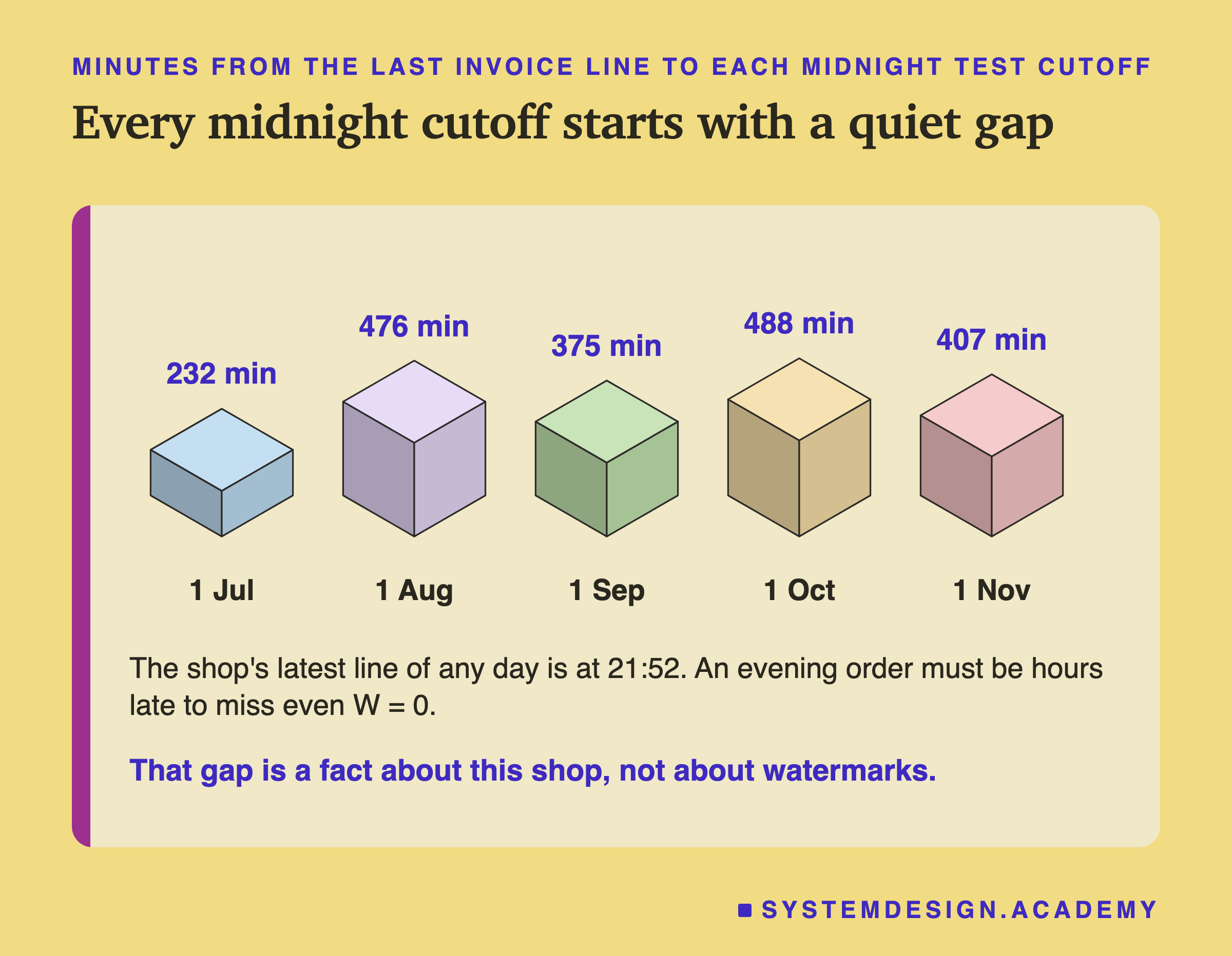
The task's cutoffs are at midnight. This shop stops recording orders in the evening: across two years, the latest invoice line of any day is at 21:52. Before the five test cutoffs, the last line came between 232 and 488 minutes before midnight.
So for the kept policy at W = 0, an order from the last evening has to be delayed for hours before it misses the cutoff. Most delays in the main model are minutes. That makes small watermarks look free here for a reason that has nothing to do with watermarks.
I saw this coming, so I wrote a second cutoff into the design before the run. It is the same kept pipeline, with features at noon of the day before, in the middle of the shop's busy hours. A later slide shows what it found.
How the Lab Was Built
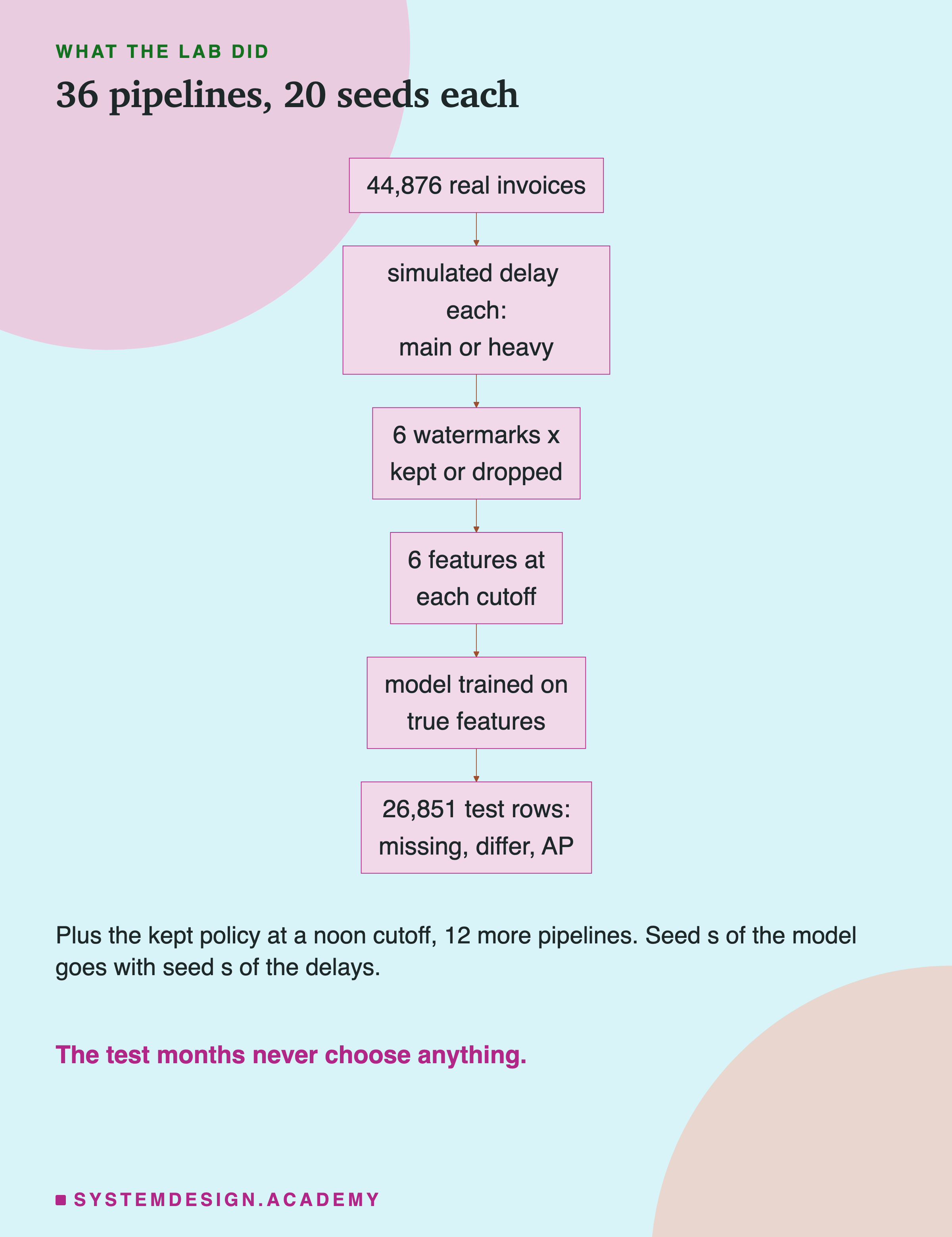
I wrote the design of the lab into the docstring of scripts/labs/features/late_events.py before it first ran. It names the delay models, the six watermarks, the two policies, the noon cutoff, what to measure, and my guesses. At that point I had looked at two things in the data. One was the hour of day of the invoices. The other was the 65 invoices whose lines carry more than one timestamp.
-
The delays. For each of 20 seeds, the lab draws one delay per invoice from each delay model. It draws them in a fixed order, so the report and the demo can draw exactly the same ones.
-
The pipelines. W takes six values: 0, 15 minutes, 1 hour, 6 hours, 24 hours and 48 hours. For each W and each policy, the lab decides which invoice lines the pipeline has at each test cutoff. Then it builds lesson 1's six features from those lines, with lesson 1's own code. A customer with no line yet gets empty features, which is what a lookup that finds no row returns.
-
The measures. For each pipeline, three numbers. The share of invoices before the cutoff that are missing. The test rows whose features differ from the true ones. And the change in test AP, against the same model served the true features.
-
The check. With true features, all 20 seeds must equal lesson 1's model exactly. They do.
My guesses, written before the run, were these. The kept policy at midnight misses well under 1 percent of invoices, and its AP change cannot be told apart from zero at any W. Dropped changes far more rows and costs a little, perhaps measurably with heavy delays at W = 0. The noon cutoff misses more at small W than midnight. One more honest note: before the full run, I ran seed 0 once to check that the code worked, and I saw its numbers. The design did not change after it.
The Lab, Rebuilt and Checked
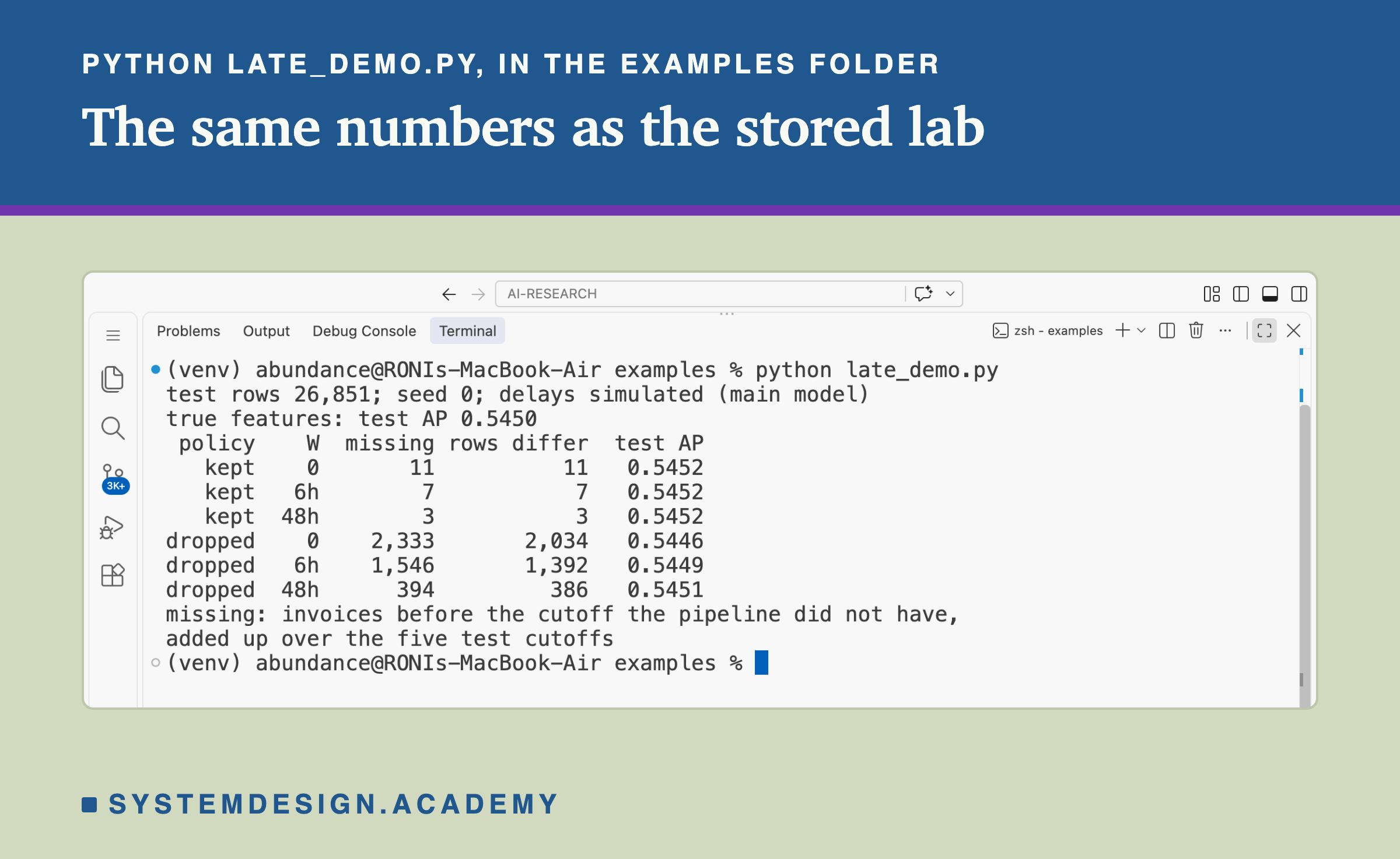
This is a real recording of the report script, late_report.py, run on the laptop where the lab ran. It does not trust the lab's code. It draws every simulated delay again with its own code, and decides with its own code which lines each pipeline has. It rebuilds every feature from the raw invoice lines, and stops on the first number that differs.
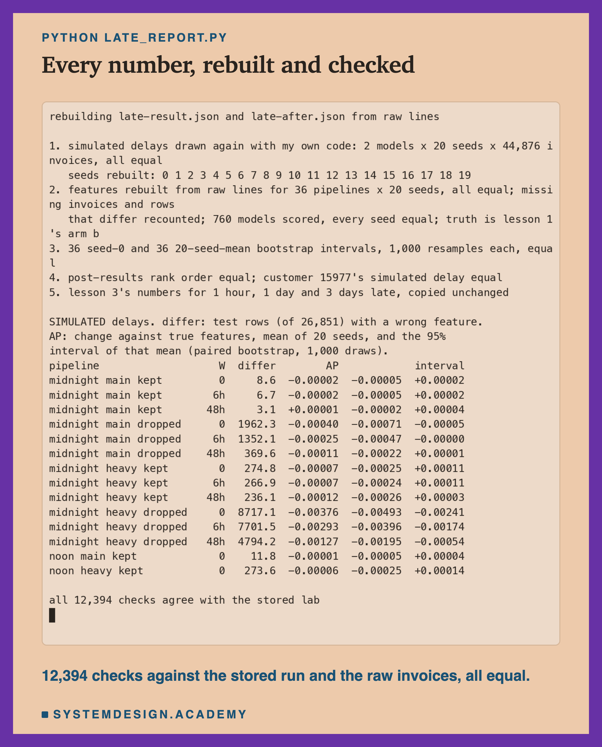
The table at the bottom is the whole result in one place. "missing" is the share of invoices before the cutoff that the pipeline did not have. "differ" is how many of the 26,851 test rows had at least one feature different from the truth, as a mean over 20 seeds. Then the change in test AP, and the 95% interval of that 20-seed mean. The recorded run took 43 minutes, while other programs were busy on the same laptop.
How Many Rows Each Pipeline Gets Wrong
Before any score, the simplest count: how many test rows have features that differ from the truth? All numbers on this slide come from simulated delays, as a mean over 20 seeds.
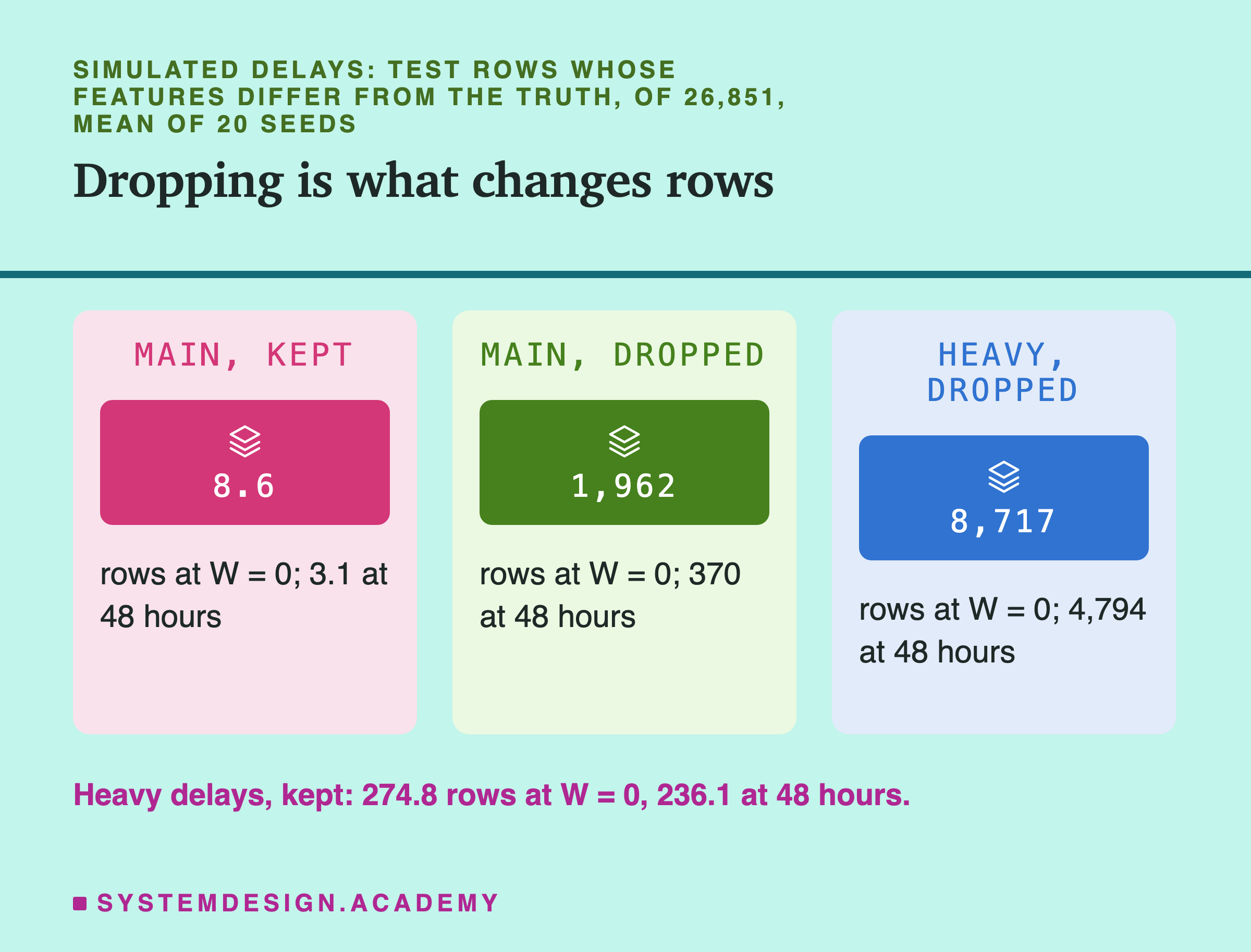
| pipeline | invoices missing, W = 0 | rows that differ, W = 0 | rows that differ, W = 48 hours |
|---|---|---|---|
| main delays, kept | 0.0047% | 8.6 | 3.1 |
| main delays, dropped | 1.24% | 1,962 | 370 |
| heavy delays, kept | 0.15% | 274.8 | 236.1 |
| heavy delays, dropped | 8.25% | 8,717 | 4,794 |
The kept policy barely touches the features. With main delays, fewer than 9 of 26,851 rows differ on average. Waiting does help, from 8.6 rows to 3.1, but there is little to fix. With heavy delays, about 275 rows differ, and waiting 48 hours fixes only about 39 of them. Why so few? The invoices still missing at T + 48 hours are the very slow tail, days or weeks late, and no watermark in this lab waits that long.
The Answer: Dropping Moved the Score; Waiting Won Back Part of It
Now the score. Each line is one pipeline. Each point is the mean change in test AP over 20 seeds, against the same models served the true features.
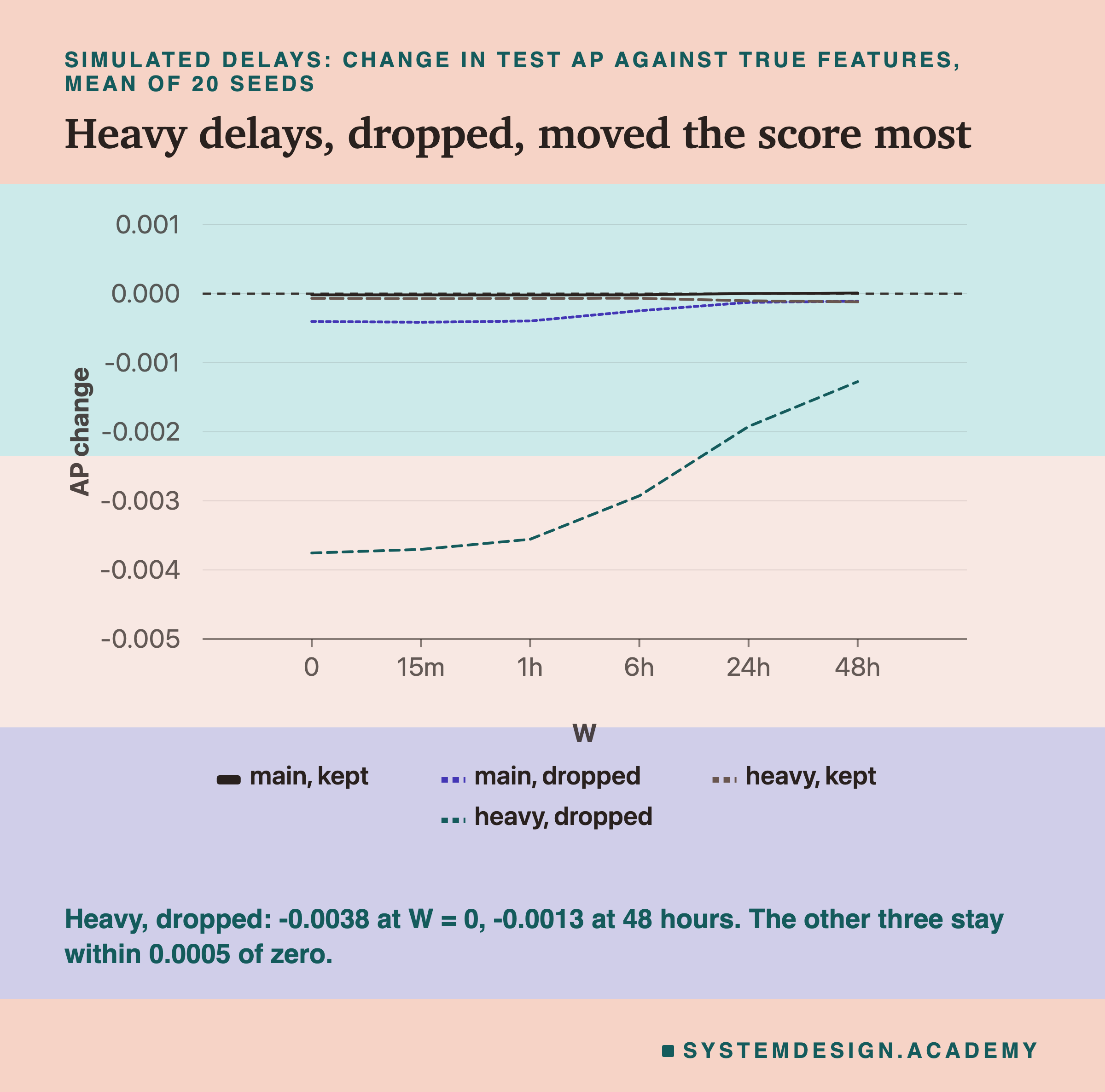
| pipeline | W = 0 | W = 6 hours | W = 24 hours | W = 48 hours | seeds below truth at W = 0 |
|---|---|---|---|---|---|
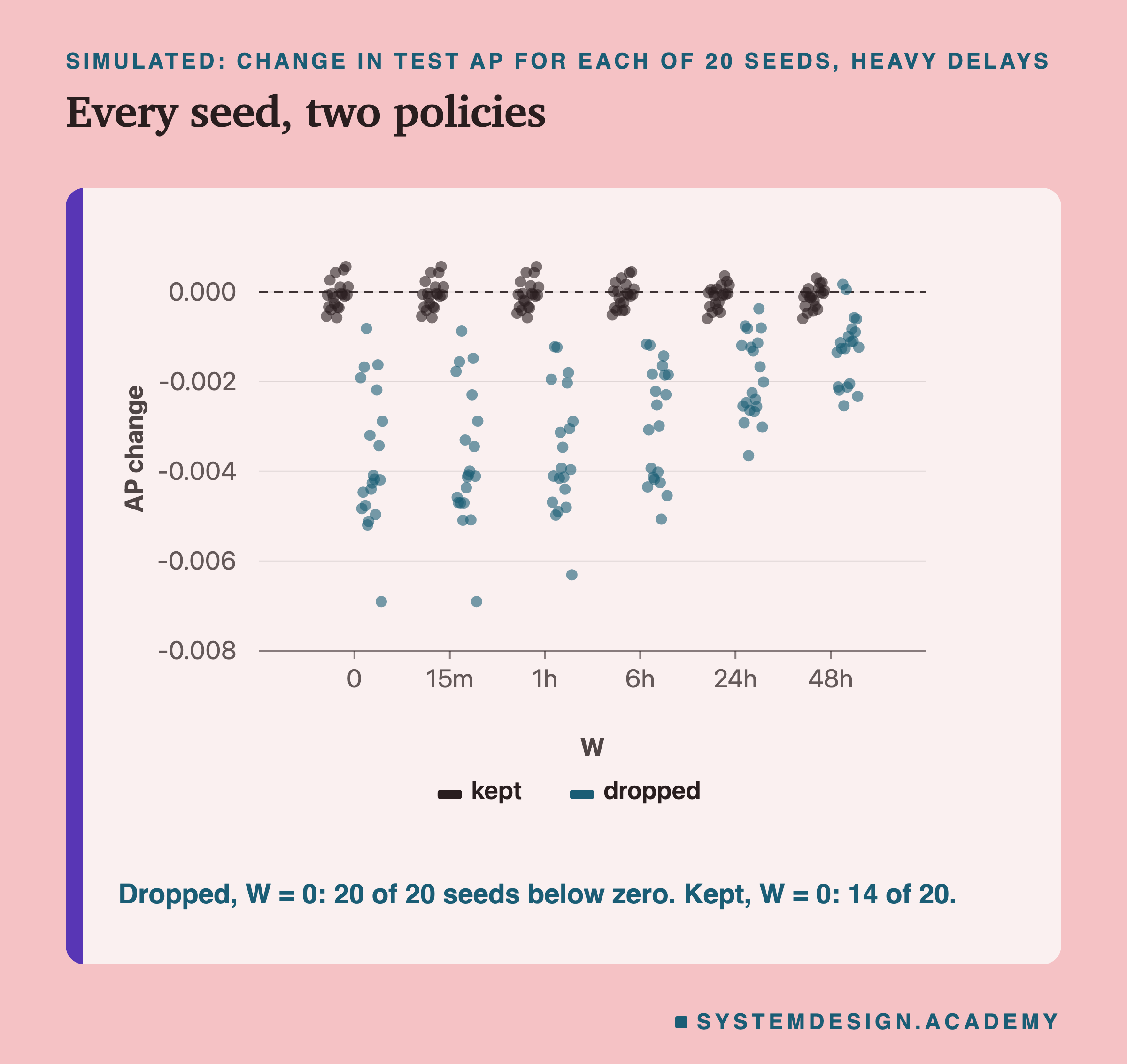
| main, kept | -0.00002 | -0.00002 | +0.00000 | +0.00001 | 12 of 20 |
| main, dropped | -0.0004 | -0.0002 | -0.0001 | -0.0001 | 17 of 20 |
| heavy, kept | -0.0001 |
Which Changes Can Be Told Apart From Zero?
Seeds and the bootstrap check different kinds of luck. The seeds move the model's training and the delay draw. The bootstrap moves which customers were tested.
While I was building this lab, a review of lessons 1 and 3 set a rule for the whole chapter. A claim that a change is or is not real must come from a bootstrap of the 20-seed mean, not of one seed. My lab's plan had only a seed 0 bootstrap. So after the main run, I added the 20-seed-mean bootstrap to the docstring, marked as added after the results, and ran it. In each of the 1,000 draws, every pipeline is scored on the same redrawn customers, and the score is averaged over all 20 seeds.
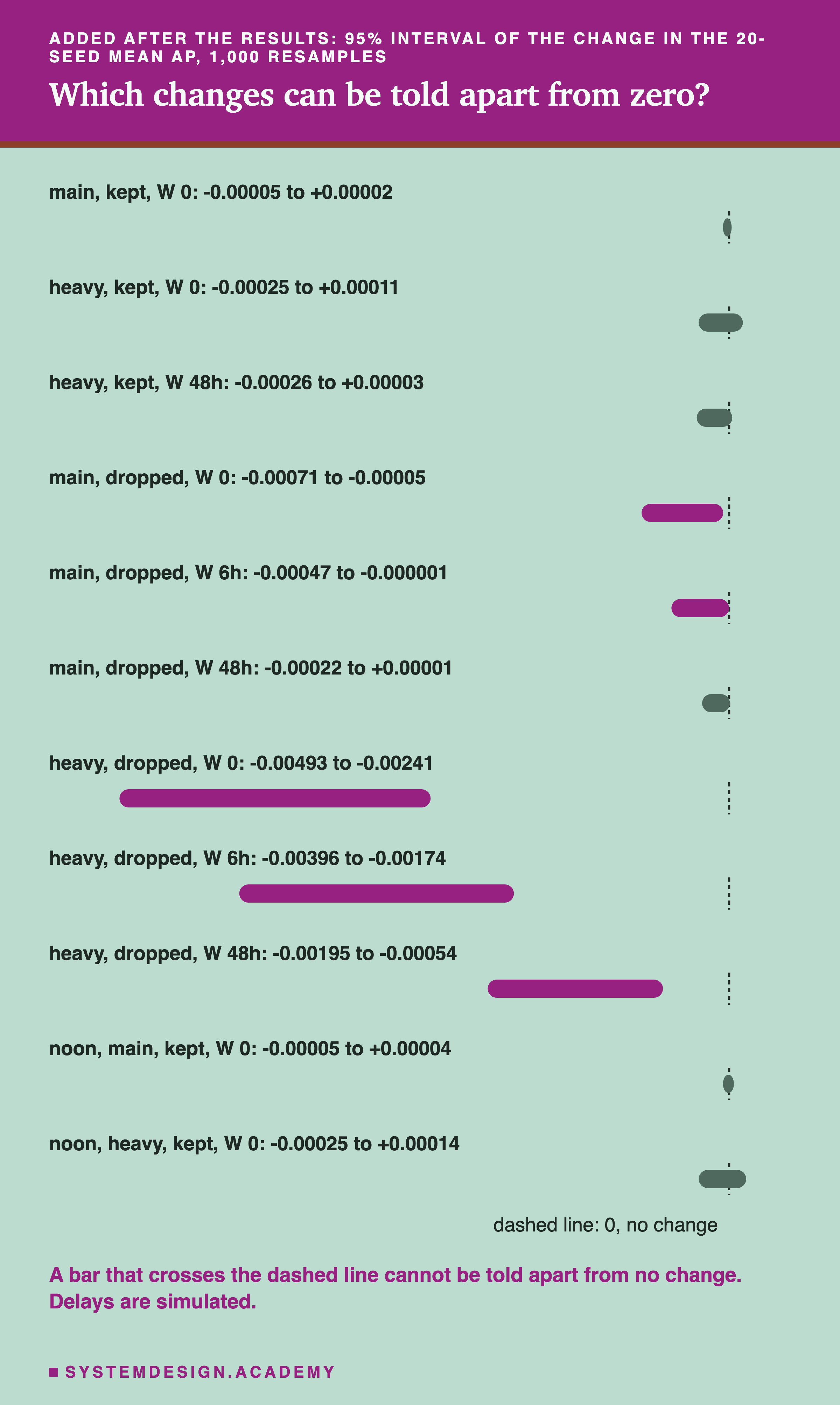
Kept. Every interval crosses zero: at every watermark, with both delay models, at both cutoffs. Waiting changed nothing that can be told apart from luck, because there was nothing measurable to repair.
Dropped, main delays. The intervals are clear of zero at W = 0, 15 minutes and 1 hour. At W = 0 the interval runs from -0.00071 to -0.00005. At 15 minutes and 1 hour, the upper ends are -0.000078 and -0.000067. At 6 hours the upper end is -0.000001, which only just misses zero, so I would not lean on it. At 24 and 48 hours the intervals cross zero.
Dropped, heavy delays. Every interval is clear of zero: -0.00493 to -0.00241 at W = 0, and still -0.00195 to -0.00054 at 48 hours.
Was It Just the Quiet Evening?
The quiet evening gave every midnight cutoff a free head start. So the noon cutoff asked: what if the cutoff fell in the busy hours instead? Same kept policy, same delays, features at noon of the day before, with its own true features and its own model.
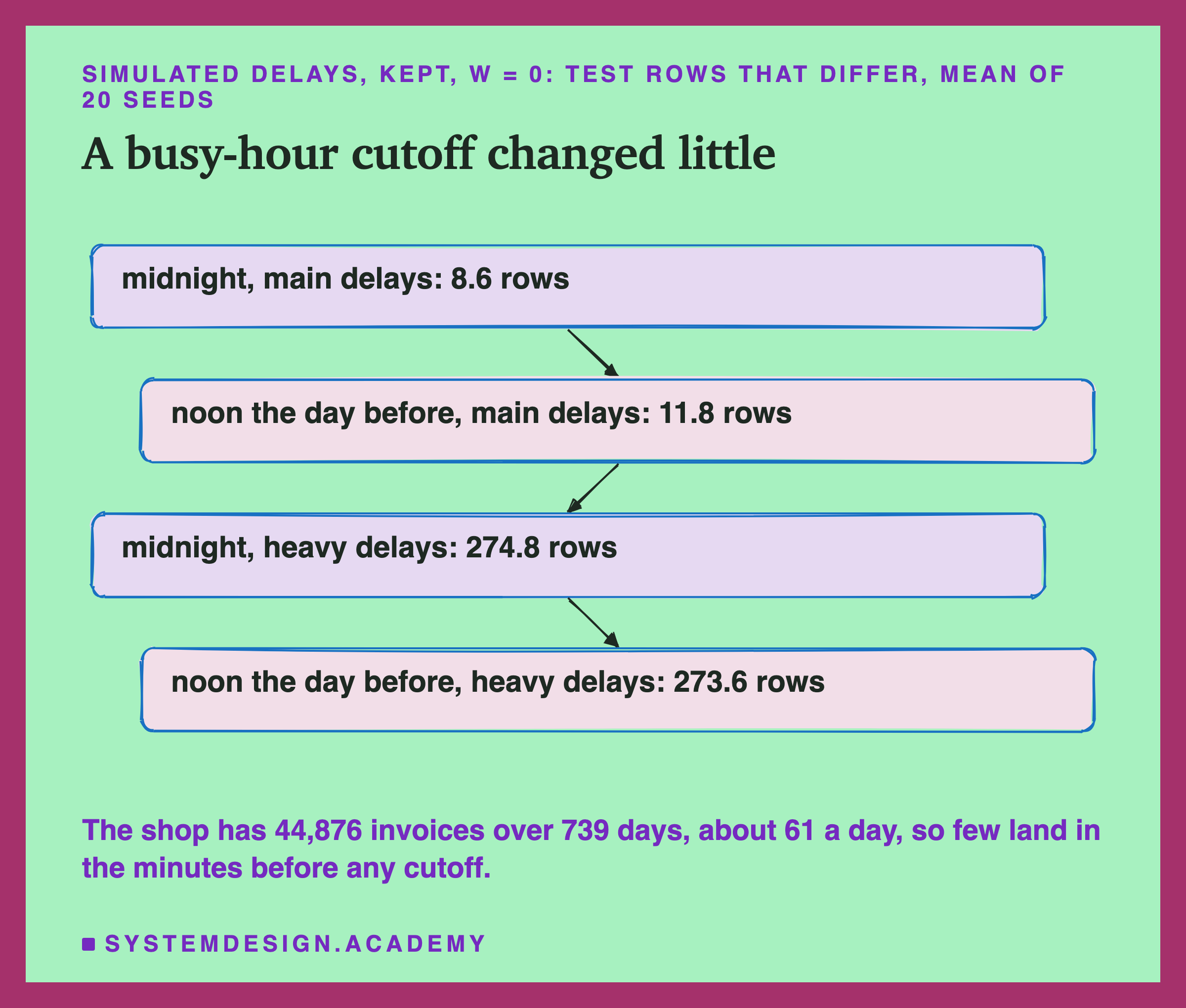
It changed little. With main delays at W = 0, 11.8 rows differ at noon against 8.6 at midnight. Among invoices from the last 24 hours before the cutoff, noon misses 3.01 percent against 1.24 percent at midnight. So the busy hours do matter for the most recent orders. Waiting 15 minutes at noon brings that down to 2.11 percent. But there are few of those orders.
One possible reason, which fits the counts: this is a small shop, about 61 invoices a day. Only a handful land in the minutes before any cutoff. Most of what the kept policy misses is the slow tail, orders hours or days late, and those are just as late whatever the hour. The AP change at noon was as small as at midnight. So the quiet evening is not why kept was nearly free here. The small number of orders near any cutoff is a likelier reason, but I did not test it on its own.
Why a Third of the Rows Moved So Little: Asked After the Results
The result surprised me a little. With heavy delays and dropped, a third of the test rows had a wrong feature, yet the score fell by only 0.0038. So after seeing the main results, I wrote one more question into the lab's docstring, and ran it afterwards. Please read this slide as a follow-up, not as part of the plan.
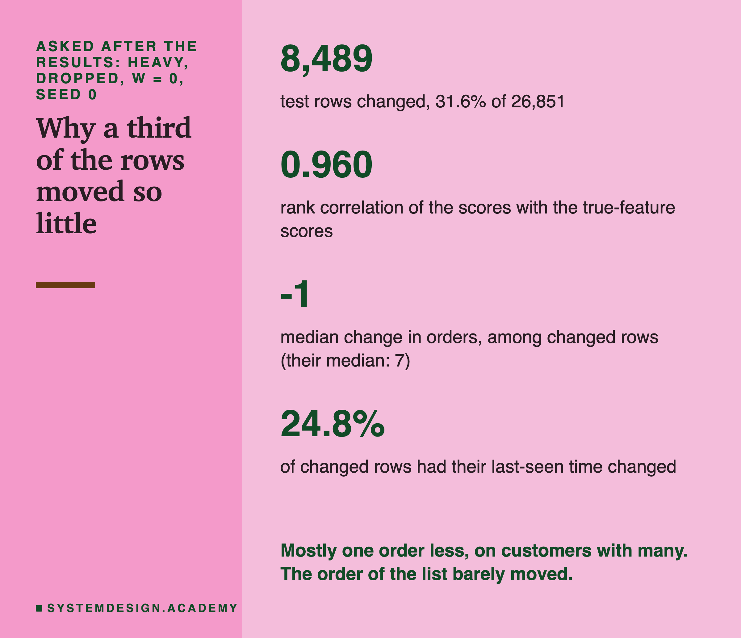
AP only cares about the order of the customers, not the exact scores. So I measured how much the order changed, with a rank correlation. A value of 1 means the two lists put every customer in the same order. A value of 0 means no relation at all. For seed 0, between the dropped pipeline's scores and the true-feature scores, it was 0.960. With main delays it was 0.993.
Then I looked at what changed in the changed rows. The median change in a customer's number of orders was -1: usually one order was lost. And these were regular customers: their median was 7 orders, against 3 for all test rows. Only 24.8 percent of them had their last-seen time changed.
One possible reason, which fits these counts: dropping takes a small share out of a long history. A customer with 7 orders who loses one still looks like a regular. I did not test this reason on its own. The changed rows were also good prospects: 32.4 percent of them bought again, against 13.9 percent of the rest. So the losses fell on the customers who matter most, and still the ranking barely moved.
What Waiting Costs: Lesson 3 Already Measured It
Waiting is not free. A result sent at T + W is a result that is W late. If the model must answer at T, it gets the features of an earlier moment instead. Lesson 3 measured exactly this staleness on this same task and model, so I did not measure it again.
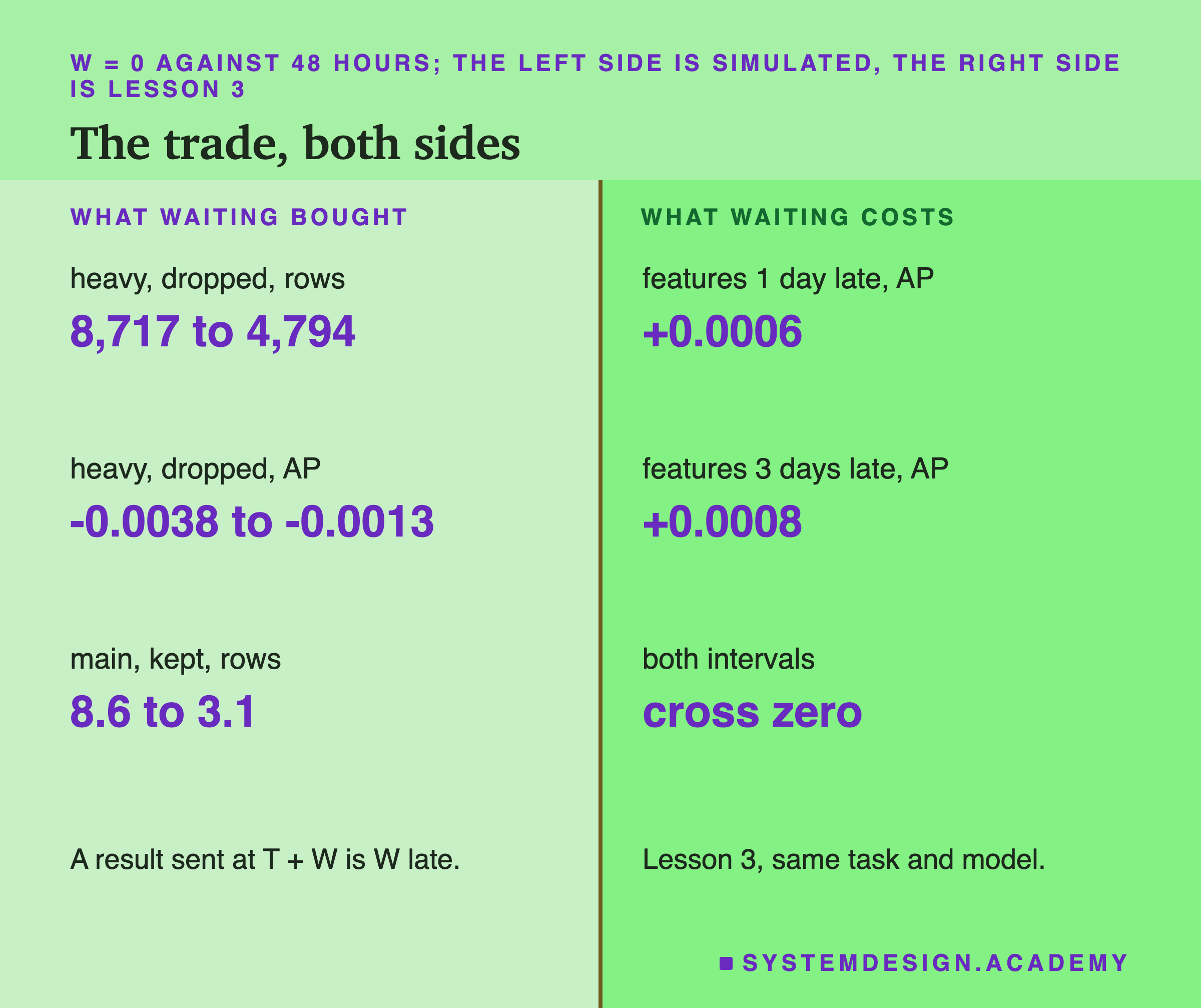
Lesson 3 served features 1 day late and 3 days late, which brackets a 48-hour watermark. The mean change in test AP over 20 seeds was +0.0006 and +0.0008, and the bootstrap of the 20-seed mean crossed zero for both. On this task, a result two days late costs nothing measurable.
So the trade here is lopsided in an odd way. Waiting costs nothing measurable, so you may as well wait. And under the kept policy, waiting also buys nothing measurable. Only a pipeline that drops late data has something to win by waiting, and even there the win is small.
In a system where the answer is needed now, the cost side changes completely. A fraud check on a card payment cannot wait 48 hours for its features. There, W is paid in money and the trade has to be measured with that system's own data.
The Lab's Code, Piece by Piece
The lab is one Python file, scripts/labs/features/late_events.py. It uses the shared file task.py for the data, the cutoffs and the labels, and imports lesson 1's feature code instead of copying it.
invoice_order and draw_delays make the simulated delays. The invoices are sorted by their first line's time, then by invoice id. A random number generator is seeded with 1000 * k + seed, where k is 0 for main and 1 for heavy. It draws three lists of the same length. The first is a uniform number per invoice, which decides whether that invoice is in the tail. The other two are a fast delay and a tail delay. The delay is the tail one when the uniform number is under the tail share.
minutes turns every time into minutes since 1 December 2009, as a plain decimal number. I did this on purpose. The heavy tail has no upper limit, and the longest delay drawn here was about 25 years. Plain minutes have no range to worry about, so the code never has to ask whether a timestamp can hold a delay.
included is the heart of the lab, two lines long. Kept: the line happened before the cutoff, and arrived by the cutoff plus W. Dropped: the line happened before the cutoff, and arrived by the end of its own day plus W.
features calls lesson 1's build_tables on only the included lines, one cutoff at a time, and joins the result onto the label rows. A customer with no included line gets empty values, written as NaN, short for "not a number". Here a feature had no missing values in training. For that case, scikit-learn's documentation says a missing value at prediction goes to whichever side of each split held more training rows.
Try It Yourself
The full lab builds 36 pipelines for 20 seeds each, 720 sets of features, and took about 17 minutes. I wrote a small demo that does the heart of it in under a minute. It uses main delays, seed 0, kept and dropped, and W of 0, 6 hours and 48 hours.
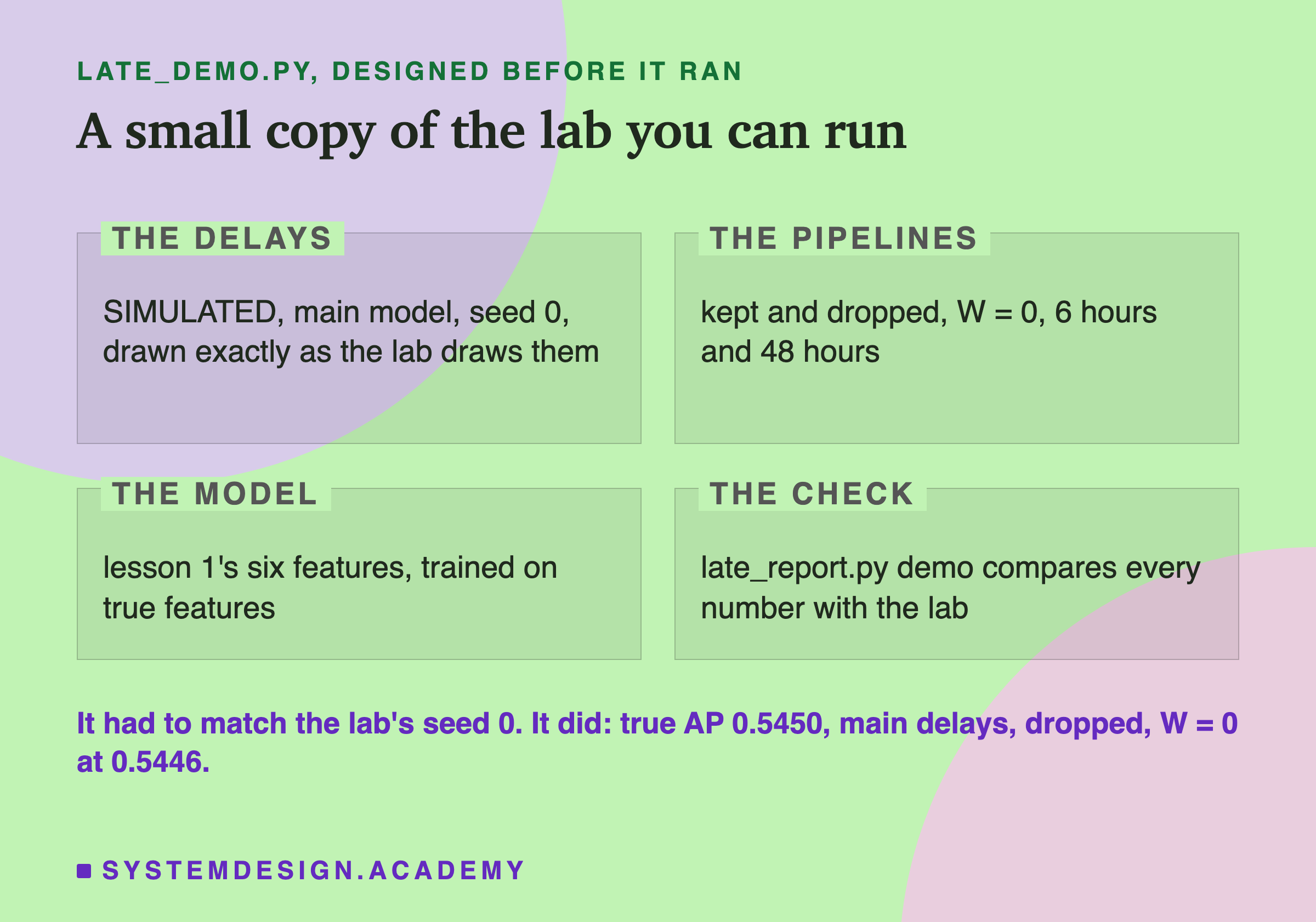
I wrote the demo's design into its docstring after the lab had run and before the demo first ran. It writes its own feature code, about twenty lines, and its own delay draw, so you can read all of it in one go.
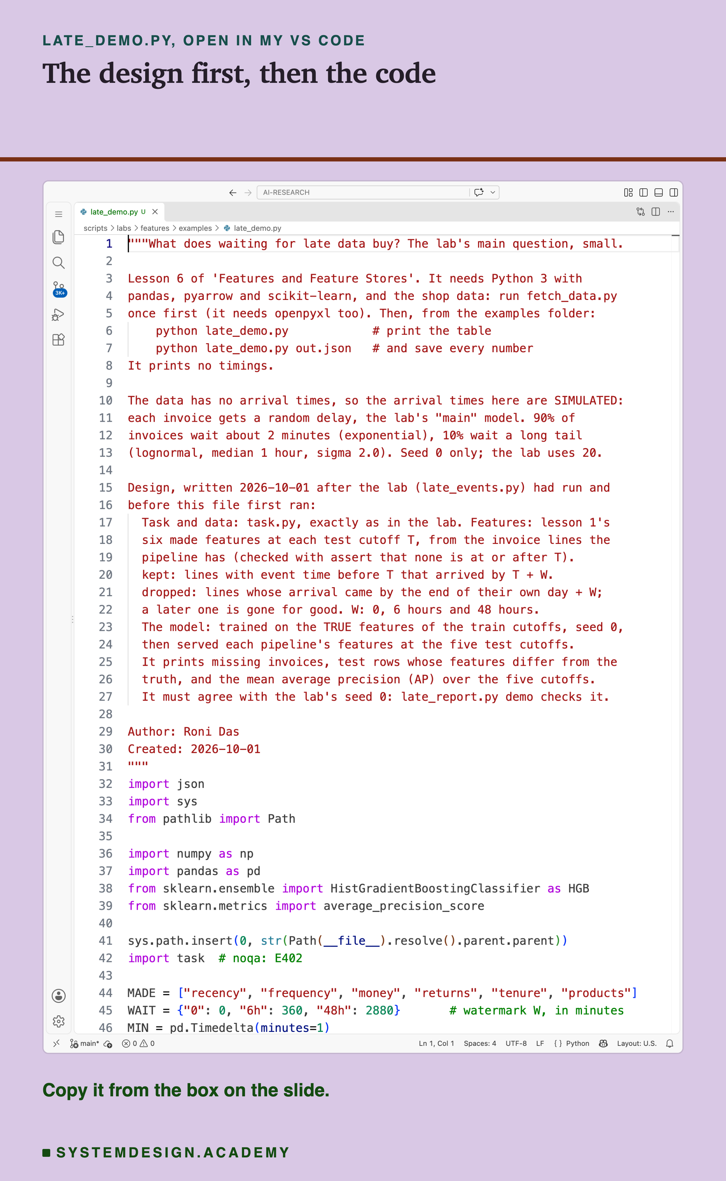
Before you run this lab. You need Python 3 with pandas, pyarrow and scikit-learn: pip install pandas pyarrow scikit-learn openpyxl. First run python fetch_data.py from the scripts/labs/features folder. It downloads the shop data once, about 46 MB, and writes one cleaned file. Then go into the examples folder and run python late_demo.py. It needs no GPU. On my Mac it took 45 seconds while other programs were also running. I ran it with scikit-learn 1.9.1 and pandas 3.0.6. These libraries run on Windows and Linux too, but I have not checked the numbers there. Give it a file name, python late_demo.py out.json, and it also saves every number. I made results/late-demo.json this way.
Move the Watermark Yourself
This box holds customer 15977's real order, the delay the lab drew for it, and the lab's mean results over 20 seeds for every pipeline. It needs nothing but Python, so it runs in your browser. Press Run to see whether the order makes it in with a 1-hour watermark.
Then change W near the top to 0, 360 or 2880 and run again. Change POLICY to "dropped", and DELAYS to "heavy", and watch the lab's line at the bottom move. The order's own fate is the same under both policies, because it is the customer's first order, from the last day.
The report script writes this box from the stored lab results. It then runs the box at all six watermarks under both policies, and checks that the order lands IN or MISSED exactly as it did in the lab.
Common Mistakes, and When Late Data Matters
Not knowing what your engine does with late data. In two of the four engines above, Flink and Beam, the default throws late events away. Streams does too, as soon as you choose no grace period. On my simulated heavy delays, that one setting changed a third of the rows, while waiting 48 hours undid less than half of it. Read your engine's default before you tune W.
Measuring rows and calling it the cost. 8,717 changed rows sounds like a disaster. It cost 0.0038 AP. A changed row and a worse ranking are different things, and you need to measure both.
Tuning a watermark on invented delays. This lab's delays are made up. Before choosing W for a real pipeline, log the arrival time next to the event time, and measure the real delays.
Believing one seed. Every delay draw is luck. The numbers here are means over 20 draws and 20 models.
When late data matters a lot. When the feature is built from the last few minutes, like payments on a card in the last ten minutes, or the clicks in a session. Then a few late events are the whole signal, and both W and the late-data policy decide whether the model sees an attack at all.
When it matters little. When the question is slow, like this one: will a customer buy within a month, asked once a month. Then a few missing orders out of a long history change little, and lesson 3 says even old features cost nothing measurable.
What This Lab Cannot Tell You
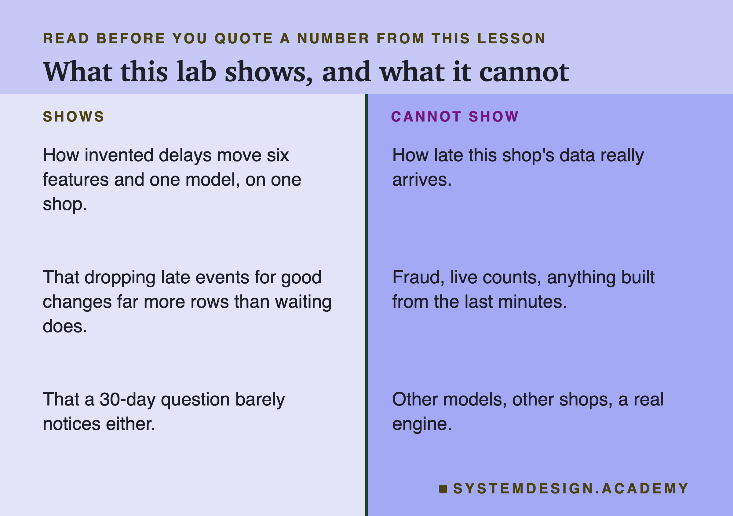
The delays are invented. This is the biggest limit, and I repeat it on purpose. The two delay models are guesses with a shape I chose. A real pipeline could be much faster, or much slower, or late in bursts, when a whole batch arrives hours late at once. My delays are independent, one per invoice. Bursts would hit many customers at the same moment.
A slow question. The label window is 30 days and the cutoffs are monthly. Lesson 3 found two weeks of staleness free on this task. A feature built from the last hour would be hurt by the same delays far more.
A simple watermark. In the lab, W is a fixed wait after a moment. A real engine works its watermark out from the event times it has seen. For example, Flink's bounded out-of-orderness takes the newest time seen minus a bound. With bursty or idle sources, a real watermark moves unevenly.
One model, trained on true features. A team that logged its live features and trained on them would teach the model what dropped rows look like. Lesson 3 tried that for staleness and it did not clearly help. I did not test it here.
A silent night. This shop records nothing from 21:52 until the next morning. A real engine works its watermark out from the event times it sees. With no events, it would stall overnight and close windows later than my fixed W. Real dropping would then be gentler than my simulation of it.
The follow-up came after the results. The 20-seed bootstrap and the question about why the cost was small were added after I saw the main results, and are labelled so.
What to Do on Monday
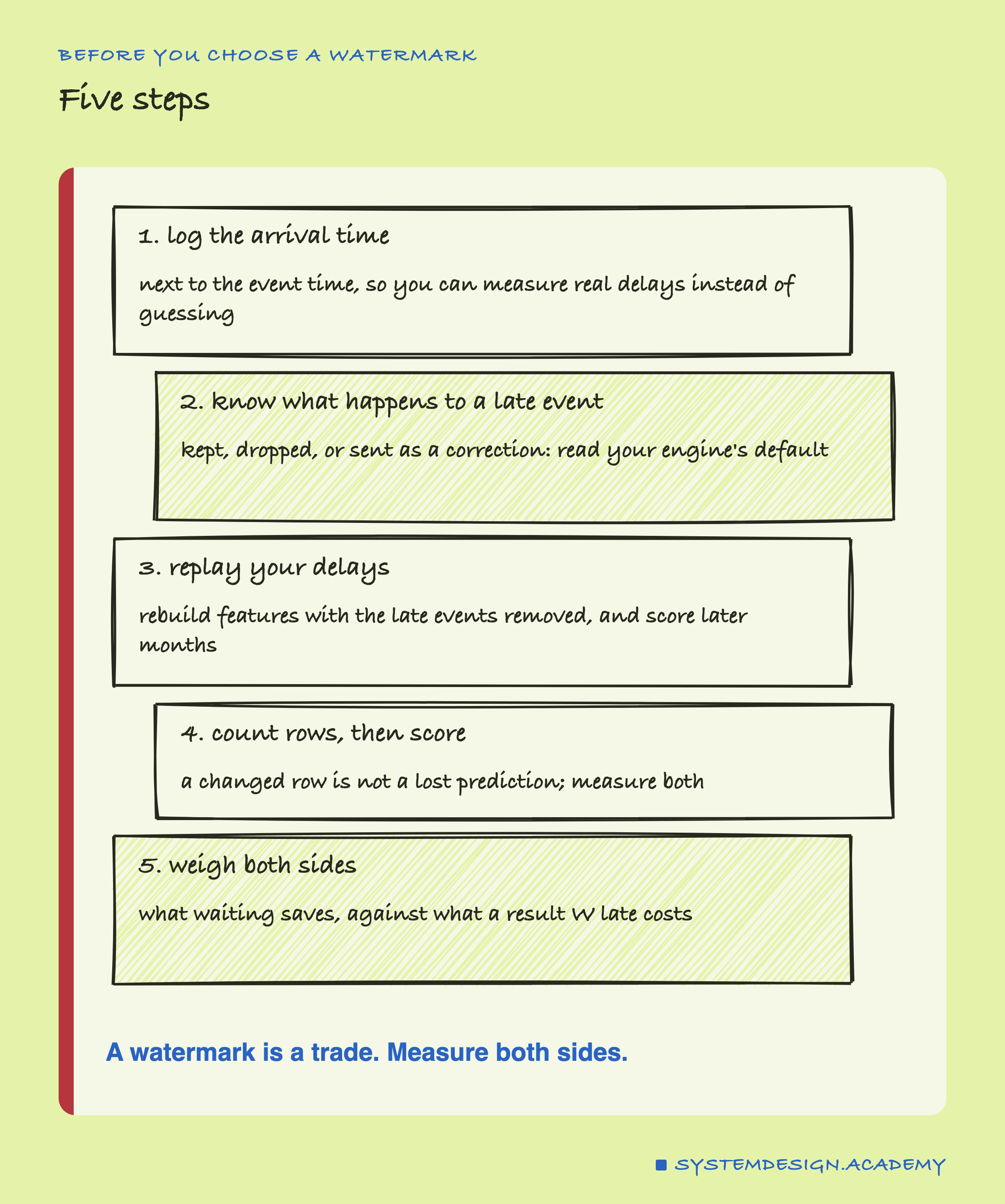
These are the five checks I would make before choosing a watermark for a feature pipeline.
-
Log the arrival time. Store when each event reached you, next to when it happened. Without it, every number in this lesson has to be simulated, and yours would be too.
-
Know the policy. Find out what your engine does with an event that arrives after its window closed: keep it, drop it, or send a correction. That choice mattered more than W here.
-
Replay your delays. Take your real delays, decide which events each W would have had at each cutoff, rebuild the features, and score later months, as this lab does.
-
Count rows, then score. Changed rows tell you where to look. The score tells you whether it matters.
-
Weigh both sides. A bigger W catches more late events, and makes every result later. Measure what lateness costs your model, as lesson 3 did.
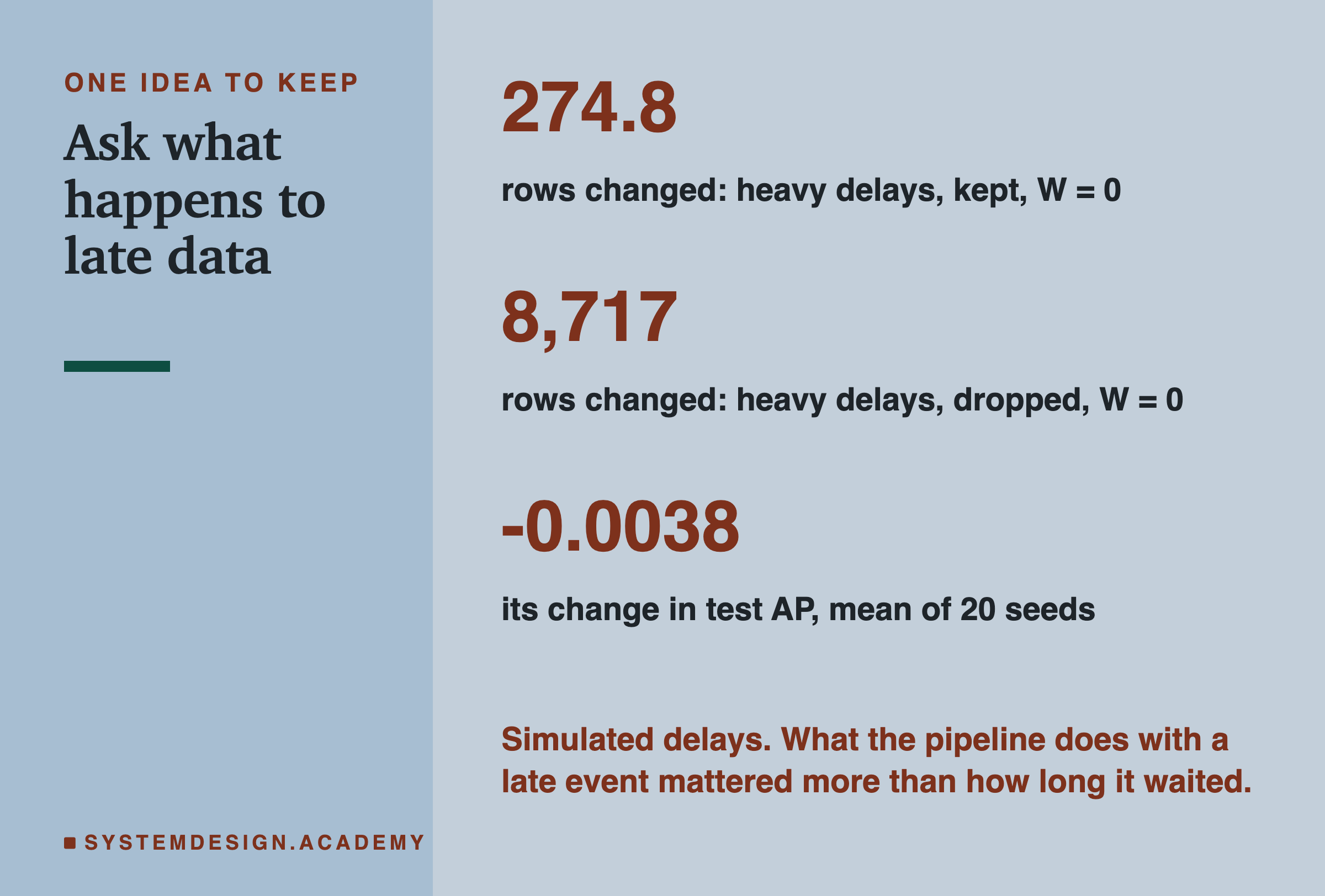
what a pipeline does with late data can matter more than how long it waits. Here, on simulated delays, keeping late events made every watermark free, and dropping them cost a small, real amount that waiting only partly won back. Measure your own delays before you trust either number.
Knowledge Check
Knowledge Check
4 questions - Score 80% to pass
Which numbers in this lesson are simulated rather than measured on the shop's data?
With heavy delays and W = 0, the dropped policy changed about 8,717 test rows and the kept policy about 275. What explains the gap?
Under the kept policy with heavy delays, waiting 48 hours fixed only about 39 of roughly 275 changed rows. Why so few?
Before choosing a watermark for a real feature pipeline, what does the lesson say to do first?