The Card in the Drawer
Let me start with a shop.
Imagine a small shop with a wall of drawers behind the counter. Each regular customer has a card in a drawer. The card says how often they come, how much they usually spend, and when they last came in. The shop owner uses the cards to decide whom to phone about a new delivery.
Nobody updates the cards after every visit. That would take all day. Instead, every Sunday evening someone sits down with the week's receipts and writes up all the cards at once.

So on a Thursday, the card she reads is four days old. A customer who came in on Tuesday and spent a lot is not on it yet. Does that matter? Would she phone the wrong people? Or are the cards still good enough, because people's habits change slowly?
This lesson asks exactly that. Machine learning systems have the same cards and the same Sunday evening. In this lesson I measure what the delay costs, on real data from a real shop.
Where This Lesson Starts
This is the third lesson of the chapter on features and feature stores. It uses the same shop data and the same prediction task as the first two.
The first lesson, what a feature is, built six made features from each customer's history: recency, frequency, money, return share, tenure and products. With those six, a default model reached a test average precision of 0.5450. I use exactly that model and exactly those features here. Lag 0 in this lesson is that model, checked to the last digit.
The second lesson, point-in-time joins, was about the opposite mistake. There, training rows read values from AFTER their cutoff, which made the offline score look far too good. Here, the live system reads values from well BEFORE its cutoff. Nothing leaks. The values are honest, only old.
The question is simple. In production, features are usually computed by a job on a schedule. At prediction time they may be hours or days old. How old can they get before the model gets worse?
The Words You Need First
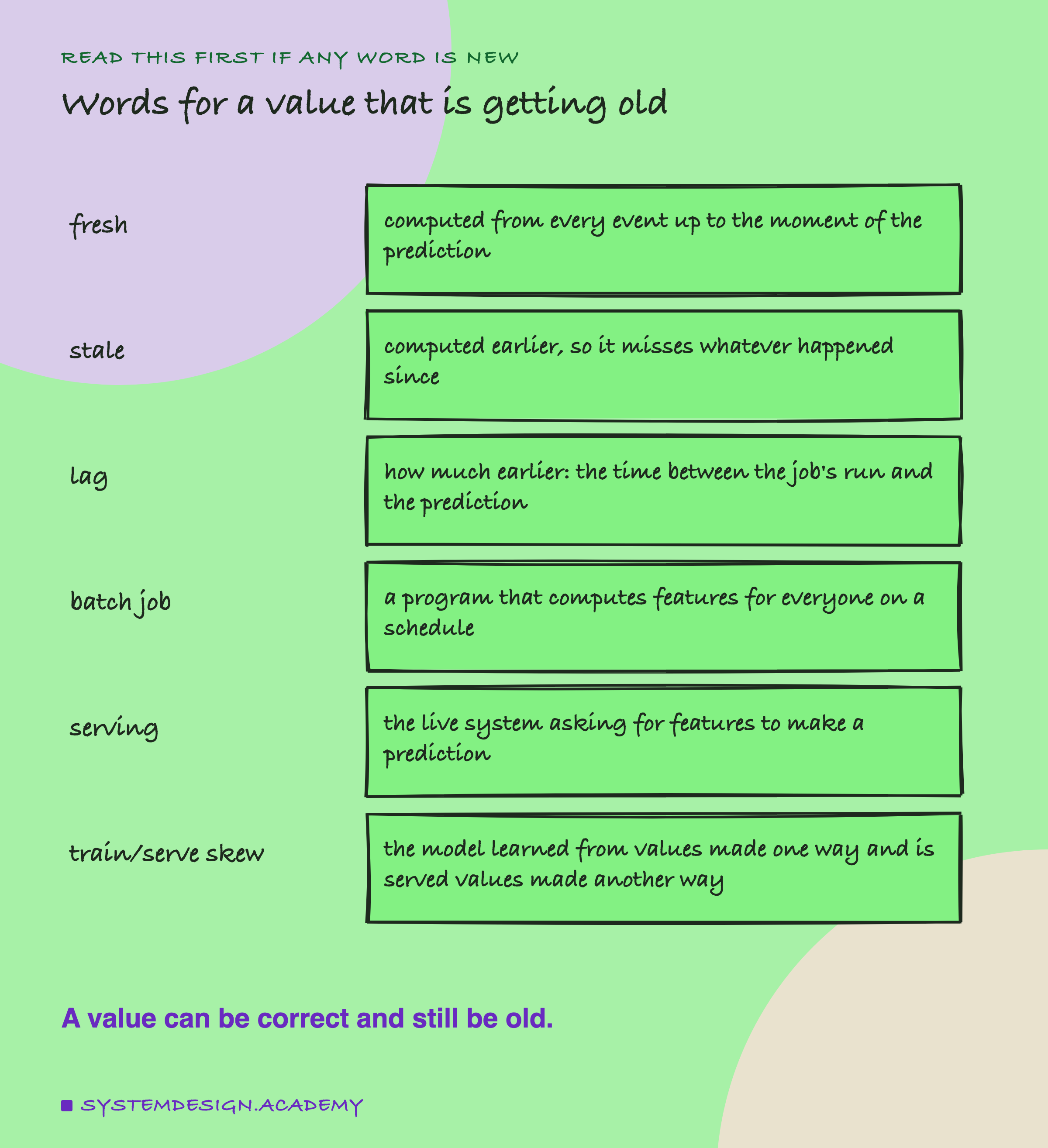
Please read this slide slowly if any word is new. Every slide after it uses these words.
Feature. One number about a customer that the model reads, like how many orders they placed. Cutoff. The moment we predict from, here the first of a month at midnight. Label. Did the customer buy in the 30 days after the cutoff, yes or no.
Fresh. A feature computed from every event up to the cutoff. Stale. A feature computed earlier, so it does not know what happened since. Think of the Thursday card.
Lag. How much earlier. If the job ran three days before the prediction, the lag is three days.
Batch job. A program that computes the features for every customer at once, on a schedule, such as every night.
Serving. The live system asking for a customer's features to make a prediction. Training. The model learning from past examples.
Train/serve skew. The model learned from values made one way, and at serving it gets values made another way. A stale feature is one kind of skew: the model learned on fresh values and now gets old ones.
How I Score a Model, and How Sure I Am
Every result slide uses these words, so here they are once more, in short.
Average precision (AP). The model gives each customer a score. Sort the customers from highest to lowest. Walk down the list, and each time you meet a real buyer, note the share of buyers so far. AP is the average of those shares. A perfect list scores 1. A random list scores about the share of buyers, which here is 0.196: the average of the five test months' shares. Counted over all test rows at once it is 0.1974, the number the demo prints. Higher is better.
ROC-AUC. The chance that a random buyer gets a higher score than a random non-buyer. A coin flip gives 0.5 and a perfect model gives 1.
Seed. A number that fixes the random choices inside training. This model keeps 10 percent of its training rows aside at random to decide when to stop, so a different seed gives a slightly different model. I train every model with 20 seeds, 0 to 19, and report the spread.
Bootstrap. A way to ask "what if the test had held slightly different customers?". Draw the test customers again at random, with repeats allowed, 1,000 times, and work out the difference each time. The middle 95 percent of those differences is the 95% interval. If it includes zero, the difference cannot be told apart from luck in which customers were tested.
Seeds and the bootstrap answer different questions. Seeds ask about luck in training. The bootstrap asks about luck in the test customers. I need both, and a later slide shows why.
One Real Customer, a Week Late
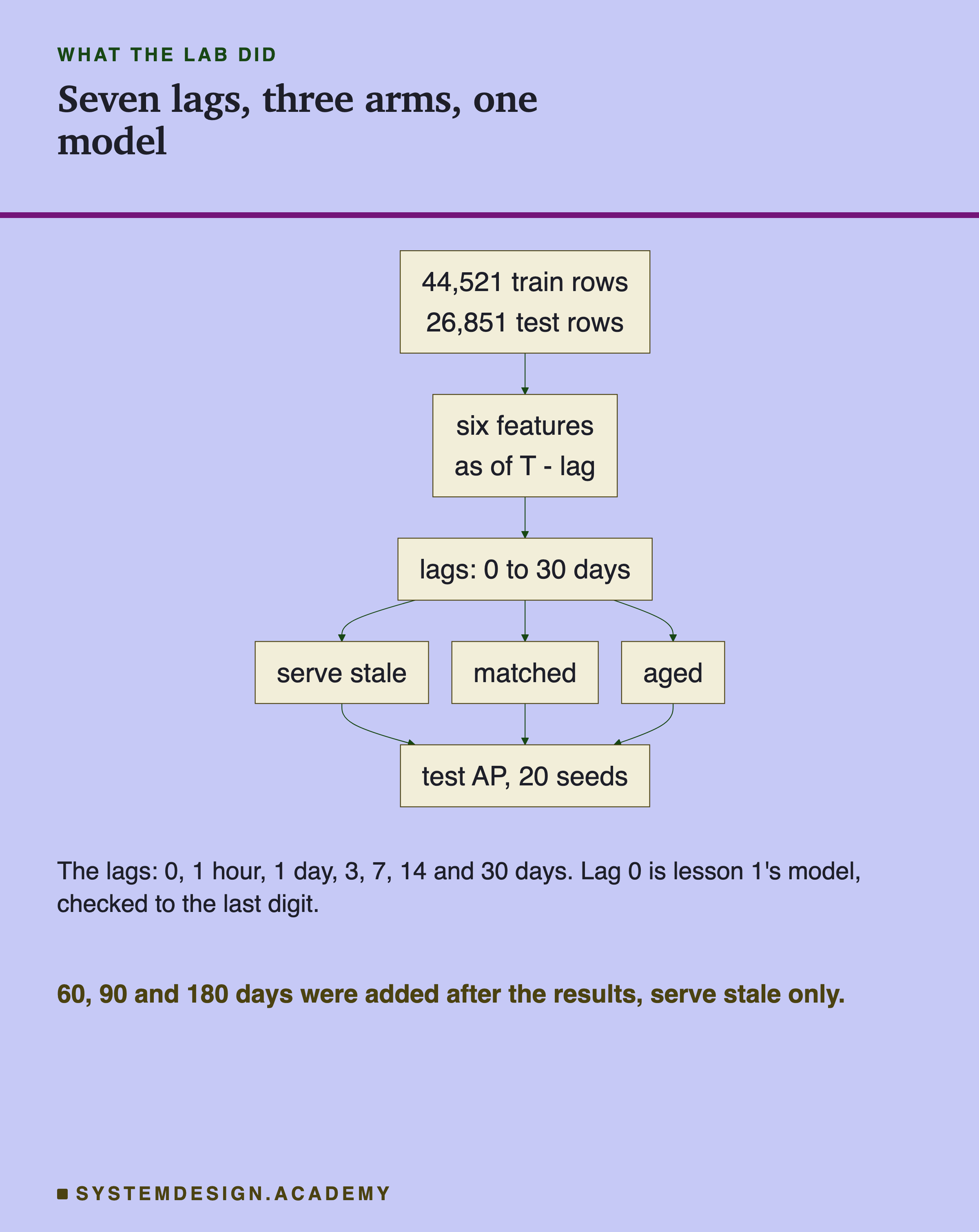
The data is UCI Online Retail II, a public dataset under a CC BY 4.0 licence. It holds the sales of a UK online shop from December 2009 to December 2011. The task is the chapter's fixed one. On the first of a month, for every customer seen before that day, will they buy again in the next 30 days? The training rows come from 13 cutoffs, 44,521 rows. The test rows come from 5 later cutoffs, July to November 2011, 26,851 rows.
Here is one real customer, number 12433, at the test cutoff of 1 November 2011. I picked them by a rule fixed before the run. The customer had to buy in the next 30 days, have an order in the last week, and have between 4 and 8 orders so far. Among the 43 who qualified, I took the smallest customer id.
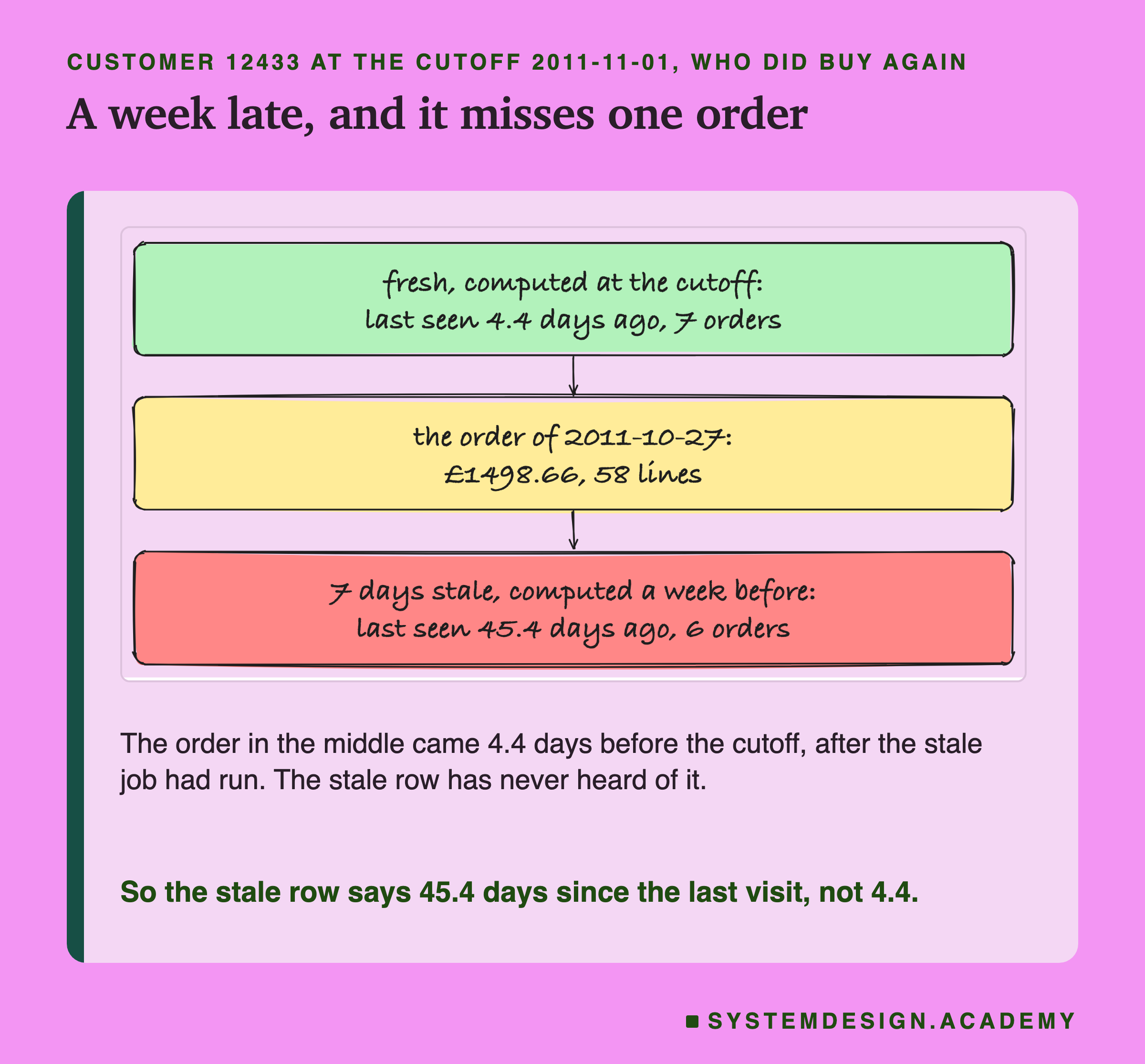
With fresh features, this customer was last seen 4.4 days before the cutoff and had placed 7 orders. With features a week stale, the job ran before their order of 27 October. So the stale row says they were last seen 45.4 days before the job ran, with 6 orders.
That is a big change for one customer. A recent, active buyer looks like someone who has not visited for six weeks. And this customer did buy again in November.
The Same Customer at Seven Lags
Here is the same customer's row at every lag the lab tests. Each row is what a job that ran that long before the cutoff would have stored.
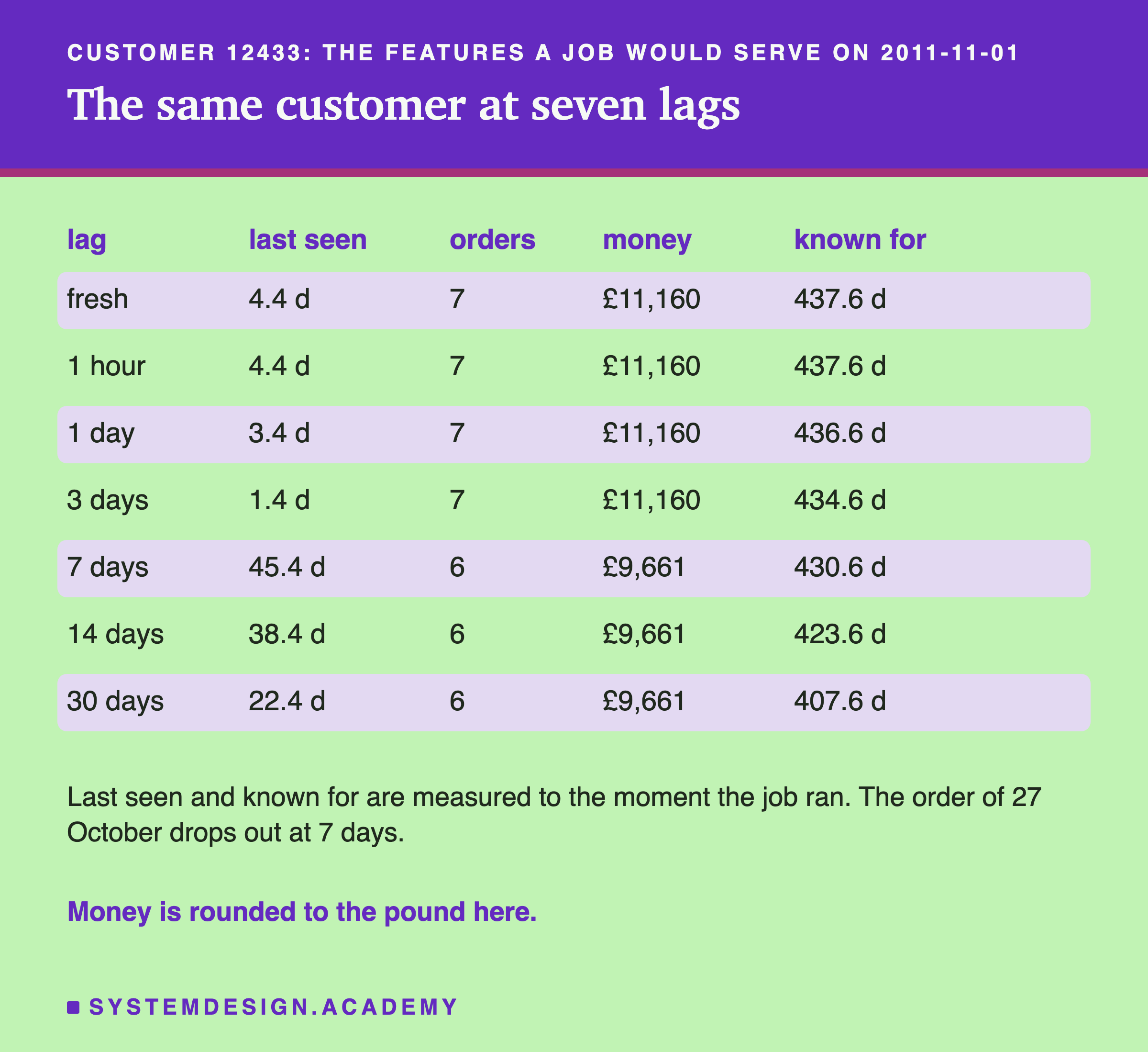
Look at the "last seen" column, which is the recency feature. It does something strange. From fresh to 3 days, it gets smaller: 4.4, 4.4, 3.4, 1.4. The job ran closer to the customer's last order, so less time had passed. Then at 7 days the order of 27 October falls out, and recency jumps to 45.4. After that it shrinks again, to 38.4 and 22.4, for the same reason as before.
This is how a stale pipeline really behaves. The job stores the numbers it computed, measured to the moment it ran, and the live system serves them unchanged. "Known for", which is the tenure feature, works the same way. Frequency and money only change when an order falls out of the window. Money here is the customer's net spend in pounds, rounded to the pound in the figure.
Where the Lag Comes From
Why would anyone serve old features? Because computing features is work, and work is usually done in batches.
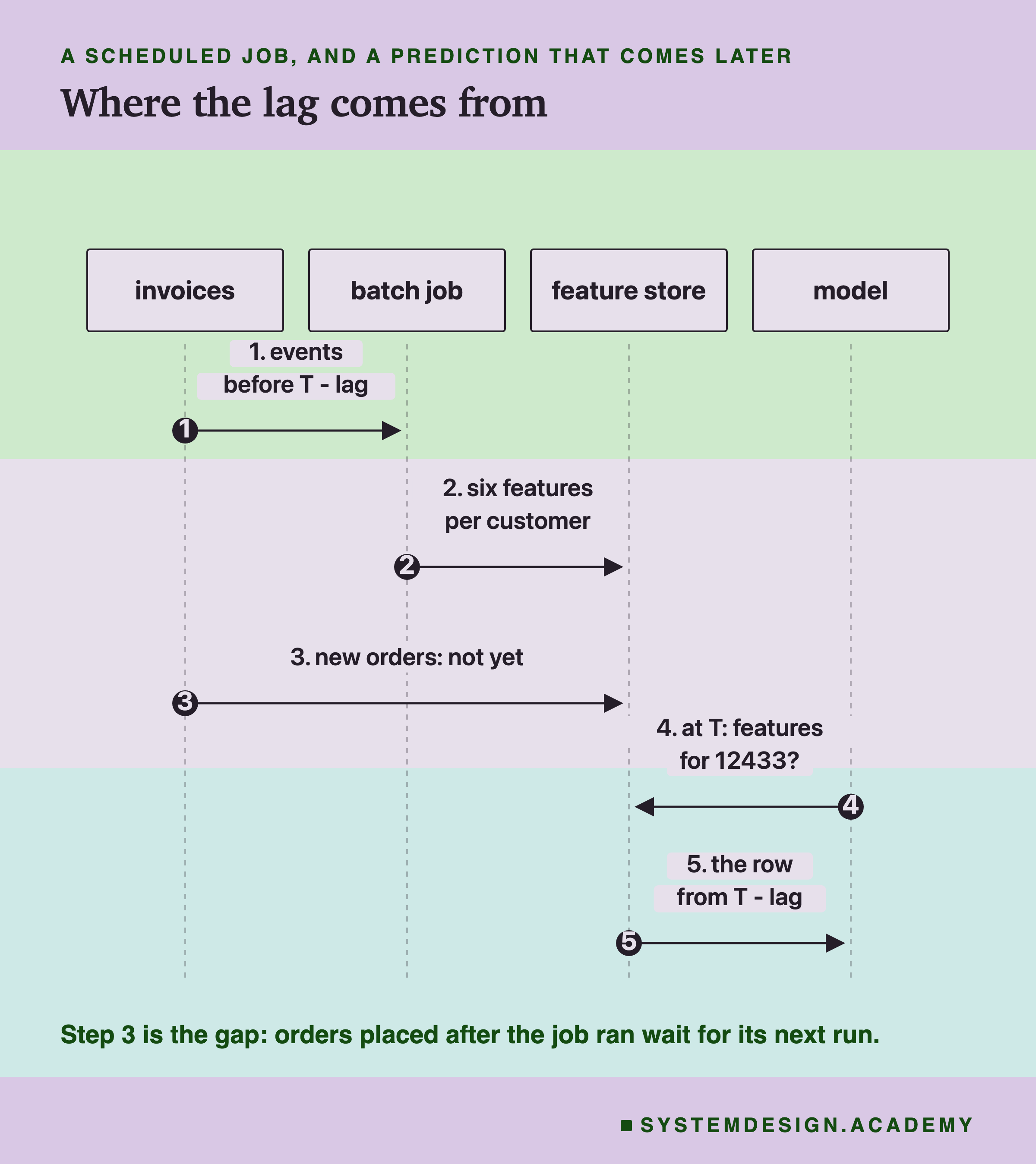
A is a system that keeps feature values for training and for serving. A common design has a batch job that reads all events, computes every customer's features, and writes them to a fast store that the live system reads from. Feast, an open-source feature store, has a step for this called materialize_incremental. To materialize here means to compute values and write them into a store, ready to be read.
Feast's documentation says materialize_incremental "fetches the latest values for all entities in the batch source" and loads them into the online store, the store the live system reads. The documentation shows it being run from Airflow, a scheduling tool. How often it runs is up to you.
Between two runs, the store holds the values from the last run. Orders placed since then wait. So the lag a prediction sees is somewhere between zero and the time between runs, plus however long the job takes. A nightly job gives lags up to about a day. A weekly job gives up to a week.
Making the job run more often costs money and effort. Before paying that, it is worth knowing what the lag costs. That is what this lab measures.
Three Ways to Live With a Lag
The lab tests three situations. I call them arms, because each one is a separate branch of the same experiment.
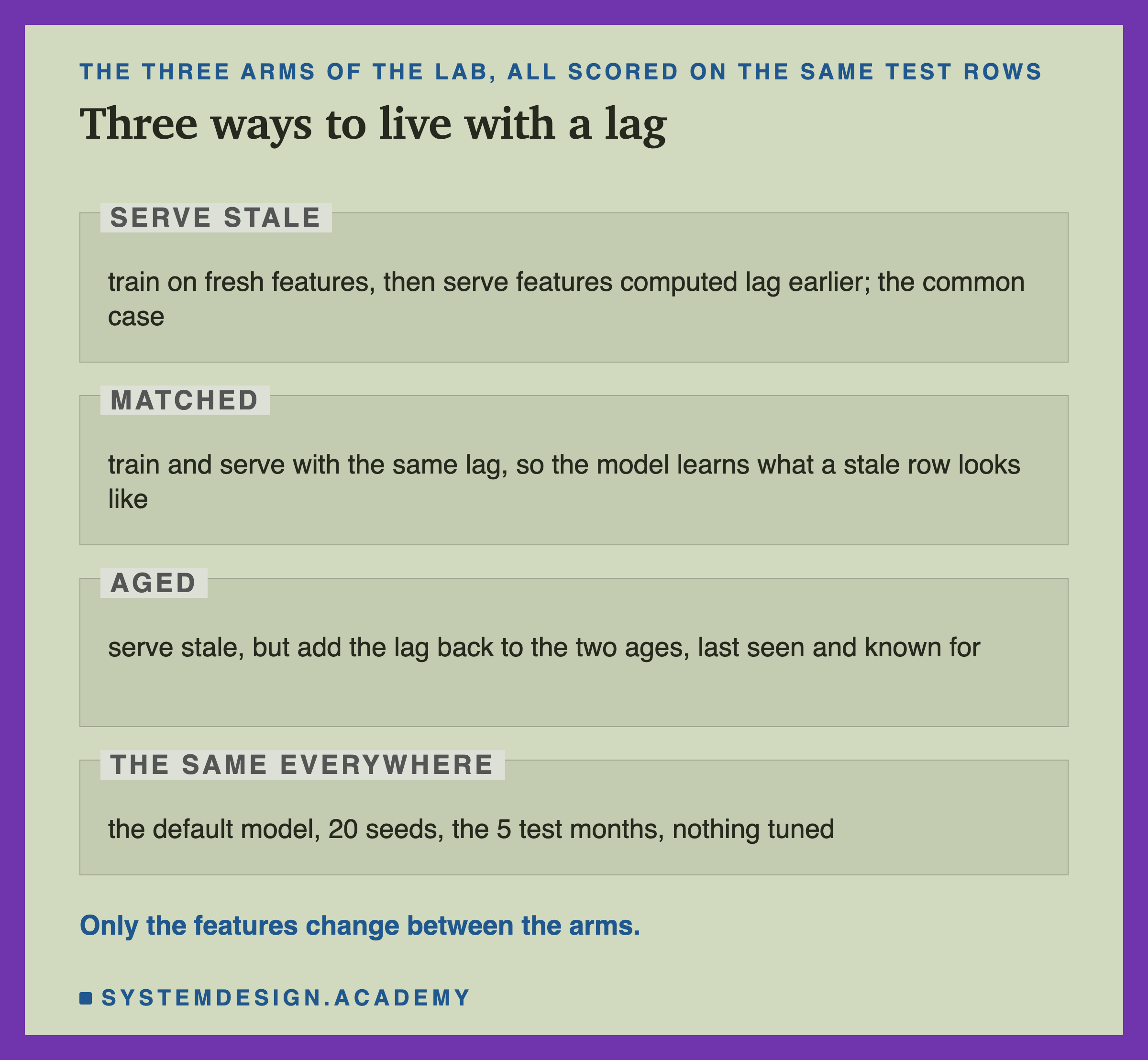
Serve stale. The model is trained on fresh features, built carefully from the past, as in lesson 1. At serving, it gets features that are a lag old. This is the common case: a team builds its training table with care, but the live system reads whatever the last job wrote.
Matched. The model is trained on features with the same lag it will see at serving. If the live system is always a week behind, train it on rows that are a week behind too. This removes the train/serve skew. What remains is only the information the lag throws away.
Aged. Serve stale, but repair the two ages. The stale row's "last seen" was measured to when the job ran. Add the lag back, so it is measured to the real prediction time. Lesson 2 gave a rule: store the time of an event, and work out the age at join time. This arm applies that rule to a stale row. I added it to the design before running. It separates two things a stale row gets wrong: its ages, which this repairs, and the orders it never saw, which nothing can repair.
How the Lab Was Built
I wrote the design of the lab into the docstring of scripts/labs/features/feature_freshness.py before it first ran. At that point I had looked at one thing in the data, the hour of day of the invoices. No model had been trained on any lag.
-
The features. For each lag, the six made features are computed as of the cutoff minus the lag, from events strictly before that moment. The lab imports lesson 1's own function for this, so the code is the same code. The rows and the labels never change.
-
New customers. A customer whose first order falls inside the lag window is in the test rows, but the stale job never saw them. Their six features are left empty, which is what a lookup that finds no row returns. At 30 days that is 716 of the 26,851 test rows.
-
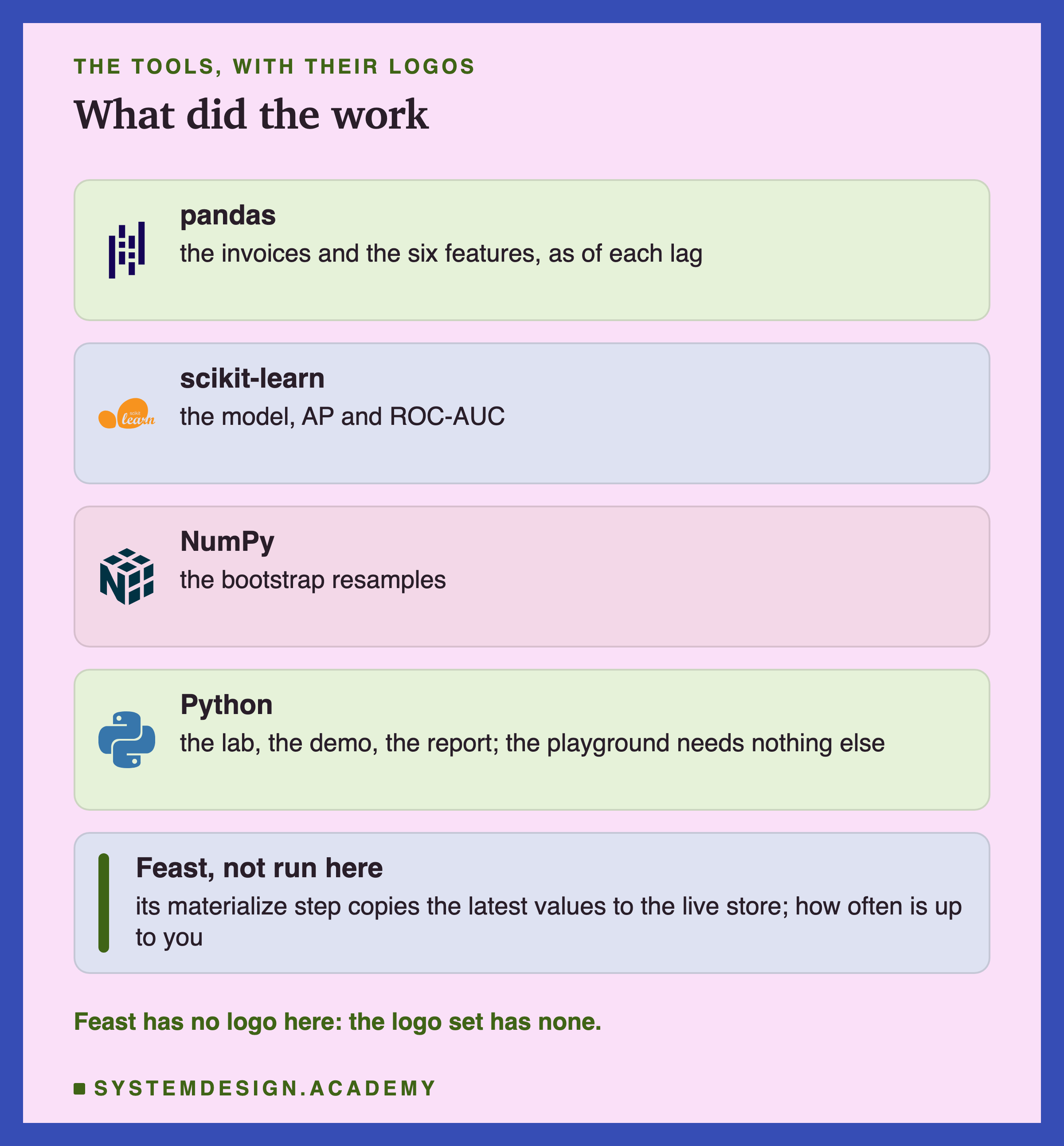
The model. HistGradientBoostingClassifier from scikit-learn with its default settings, the same as lesson 1. It is a gradient boosting model. It builds many small decision trees one after another, and each new tree tries to fix the mistakes of the ones before. Nothing is tuned.
-
The check. Lag 0 must give lesson 1's numbers exactly. It does, on all 20 seeds: seed 0 scores 0.5450.
I also wrote down my guess. One hour would cost nothing, because the shop records no order after 22:00. One to three days would cost too little to see. Thirty days would cost clearly. It would cost more in AP than in ROC-AUC. Matched would cost less than serve stale. Aged would win back part of the loss. The last four guesses turned out wrong, the first of them only partly: thirty days did cost something, but not clearly, as later slides show.
The Lab, Rebuilt and Checked
This is a real recording of the report script, fresh_report.py, run on the laptop where the lab ran. It does not trust the lab's code. It rebuilds every feature at every lag from the raw invoice lines with its own code, and stops on the first number that differs.
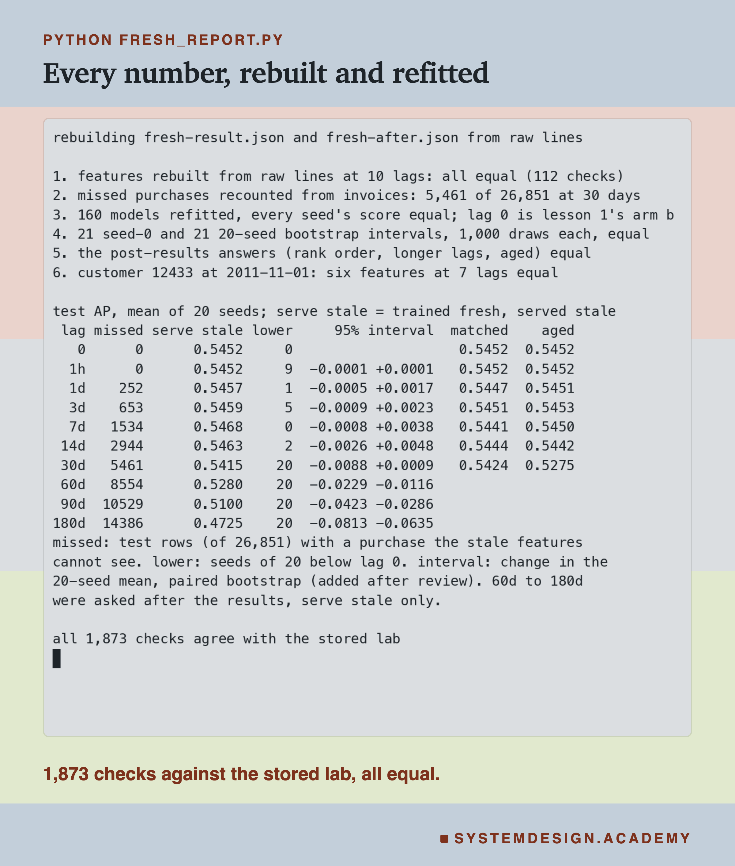
The report then refits all 160 models with the same seeds and checks every stored score. It also checks both kinds of bootstrap interval, and every number I asked after the results or after the review. It also checks that the missed orders, counted from invoices rather than lines, match the lab's count.
In the table, "missed" is the number of test rows with an order inside the lag window. "lower" is how many of the 20 seeds scored below lag 0. The 95% interval is the bootstrap of the 20-seed mean, added after the review. The rows from 60 days down were added after I saw the results, which the next slides explain.
What Each Lag Hides
Before any score, the simplest count. How many test customers placed an order inside the lag window, an order the stale features cannot see?
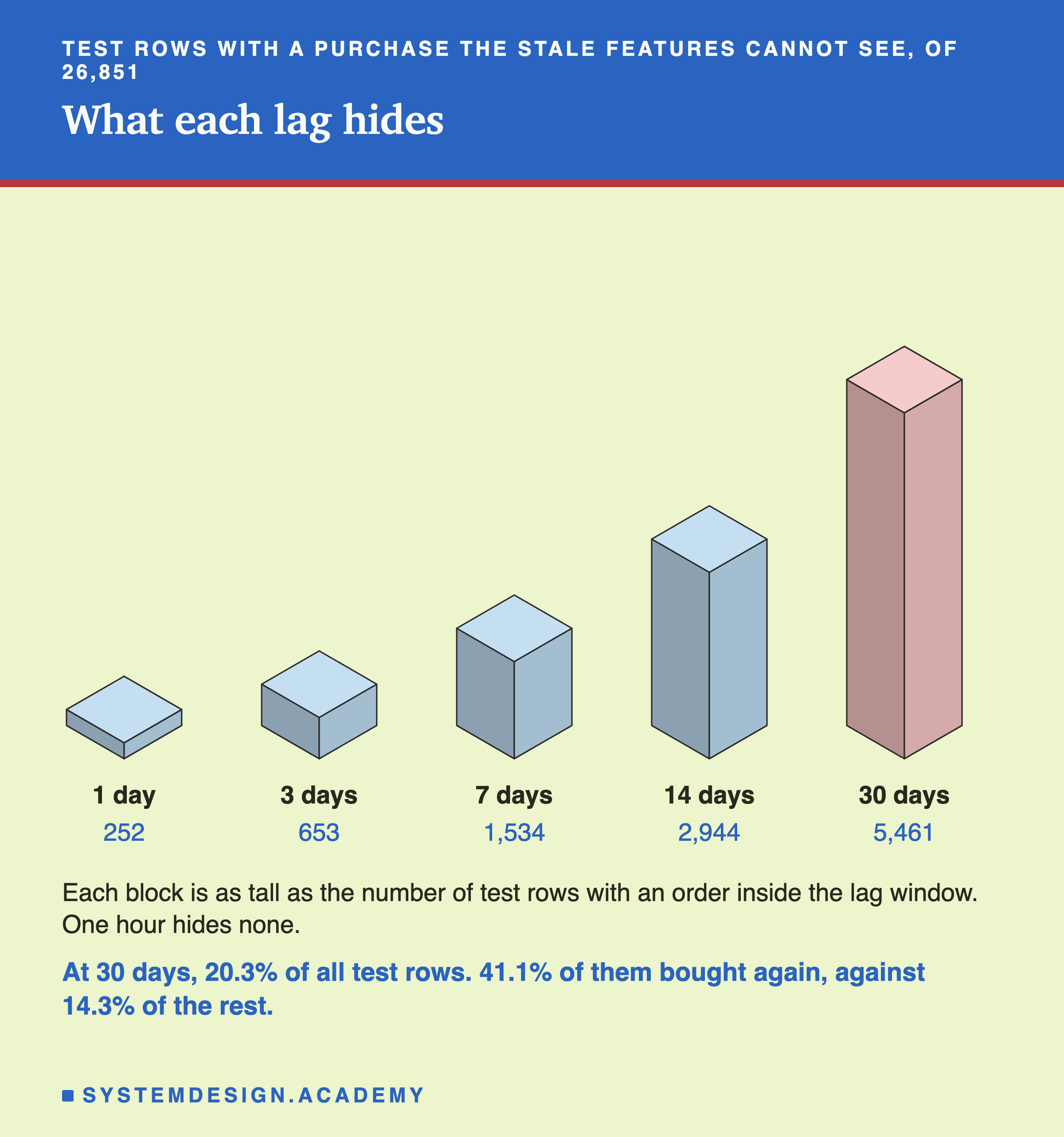
One hour hides nothing at all. The cutoff is midnight, and the shop has no order line at 22:00 or later, so the last hour of every month is empty. That result is true by construction, not a finding. Only the two ages move, recency and tenure, each by one twenty-fourth of a day: customer 12433's tenure goes from 437.609 to 437.567 days.
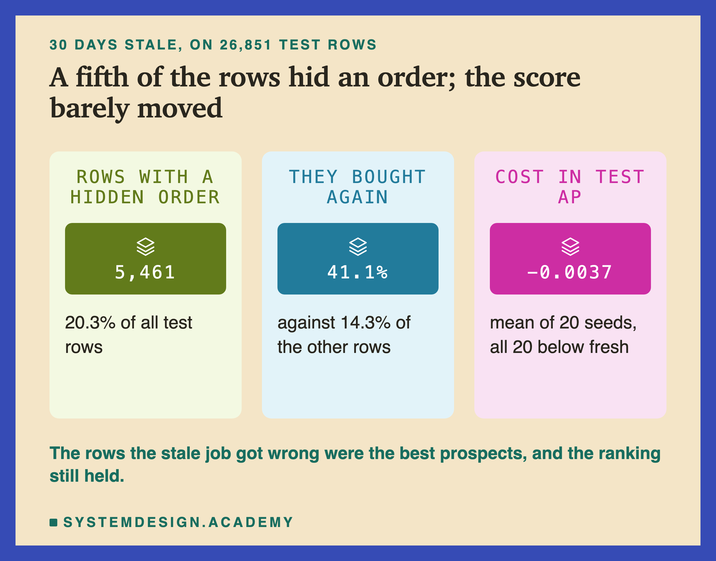
From there the count grows steadily. One day hides orders from 252 test rows. A week hides 1,534. Thirty days hides 5,461, which is 20.3 percent of all test rows.
And these are not random customers. Of the rows with a hidden order at 30 days, 41.1 percent bought again in the label window. Of the other rows, only 14.3 percent did. The stale job is wrong exactly about the customers most likely to come back. So I expected a clear cost.
The Answer: Flat for Two Weeks
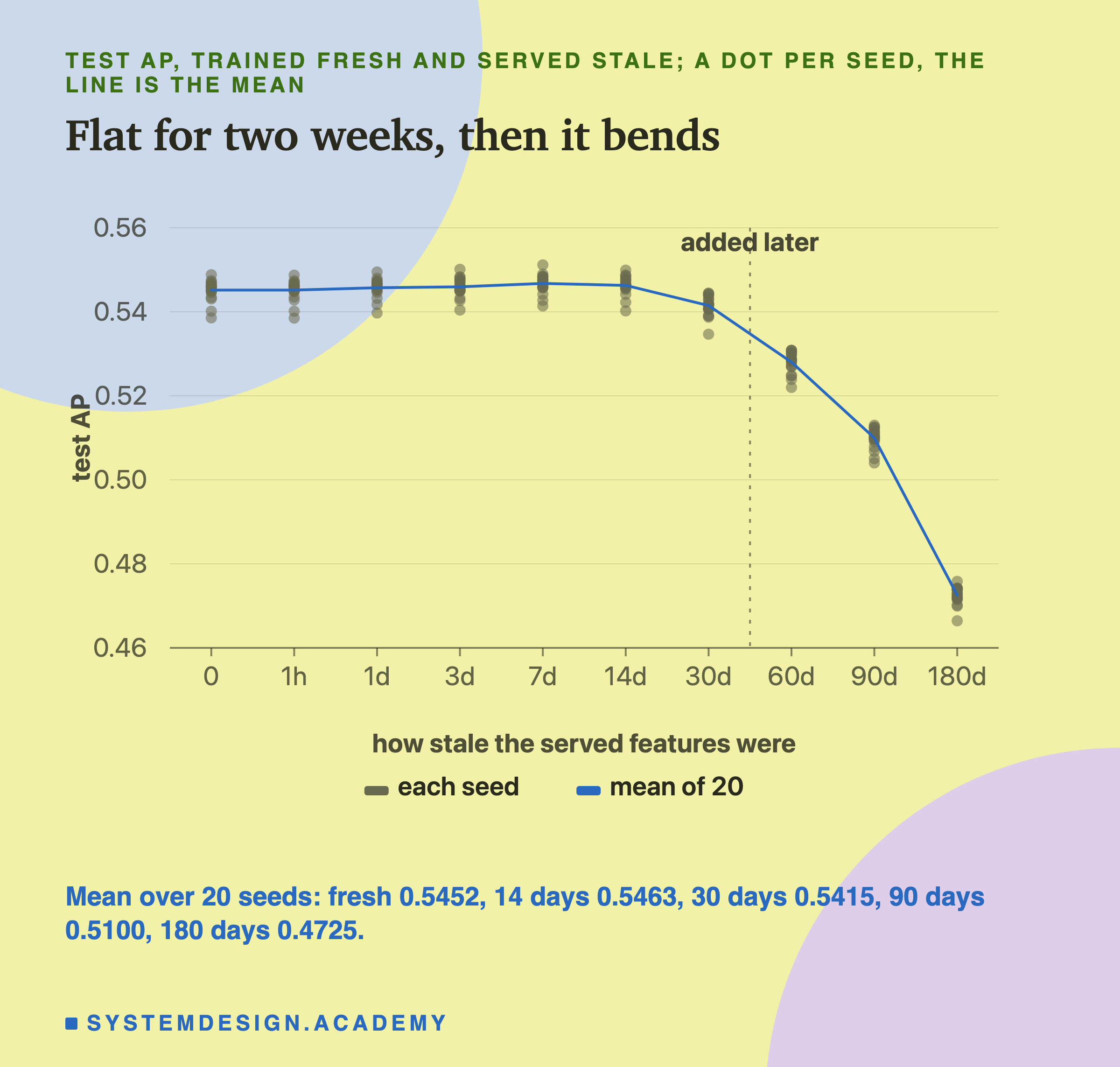
Here is the headline. Each dot is one of the 20 seeds. The line is their mean.
| lag | test rows with a hidden order | serve-stale test AP, mean of 20 seeds | seeds below fresh |
|---|---|---|---|
| fresh | 0 | 0.5452 | |
| 1 hour | 0 | 0.5452 | 9 |
| 1 day | 252 | 0.5457 | 1 |
| 3 days | 653 | 0.5459 | 5 |
| 7 days | 1,534 | 0.5468 |
Which Lags Can Be Told Apart From Zero?
The table says 7 days scored higher than fresh in all 20 seeds, and 30 days lower in all 20. Are those real? The seeds only test luck in training. A bootstrap tests luck in which customers were tested. I need both.
My first version of this slide used a bootstrap of the seed 0 model alone. An independent review of the draft pointed out the problem. The lesson quotes the mean of 20 seeds, and seed 0 lost more at 30 days, 0.0059, than the mean did, 0.0037. So after that review I added a second bootstrap, of the 20-seed mean itself, and this slide now uses it. It is paired: in each of the 1,000 draws, every lag is scored on the same redrawn customers, so the comparison is fair draw by draw.
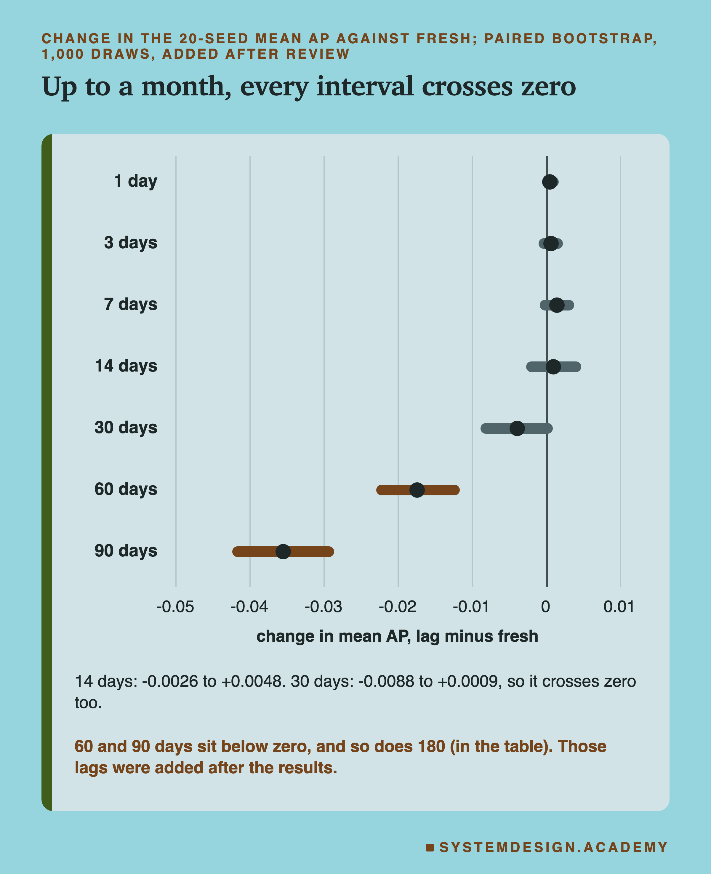
For 7 days the 95% interval of the change in the mean ran from -0.0008 to +0.0038. For 14 days, from -0.0026 to +0.0048. Both include zero, so both cannot be told apart from no change.
Thirty days ran from -0.0088 to +0.0009. That includes zero too. So here is what I can say about a month. All 20 seeds were below fresh, so luck in training is ruled out. But with these customers, the size of the loss cannot be pinned down, and the interval crosses zero. The seed 0 bootstrap alone, -0.0113 to -0.0005, would have told me it was settled. It was not. Only at 60 and 90 days does the interval sit clearly below zero.
Why were all 20 seeds above fresh at 7 days, then? Every seed was scored on the same 26,851 customers. If something about those particular customers favours the week-old values a little, every seed sees it. A different set of customers could flip it. I did not test what that something is. The point is narrower: agreement across seeds does not prove a gap is real, because all the seeds share one test set.
Why So Small? Asked After the Results
The main result surprised me. A fifth of the test rows had an order the stale features never saw, and those were the best prospects. Yet a month of staleness cost only 0.0037. I wrote three new questions into the lab's docstring after seeing the main results, and before they ran. Everything on this slide and the next one comes from that later run, so please read it as a follow-up.
The first question was about the ranking. AP only cares about the order of customers, not the exact scores. So I measured how much the order changed, with a rank correlation. A value of 1 means the stale features put every customer in the same order as the fresh ones. A value of 0 means no relation at all. At 30 days it was 0.952 for the seed 0 model. The order barely moved.
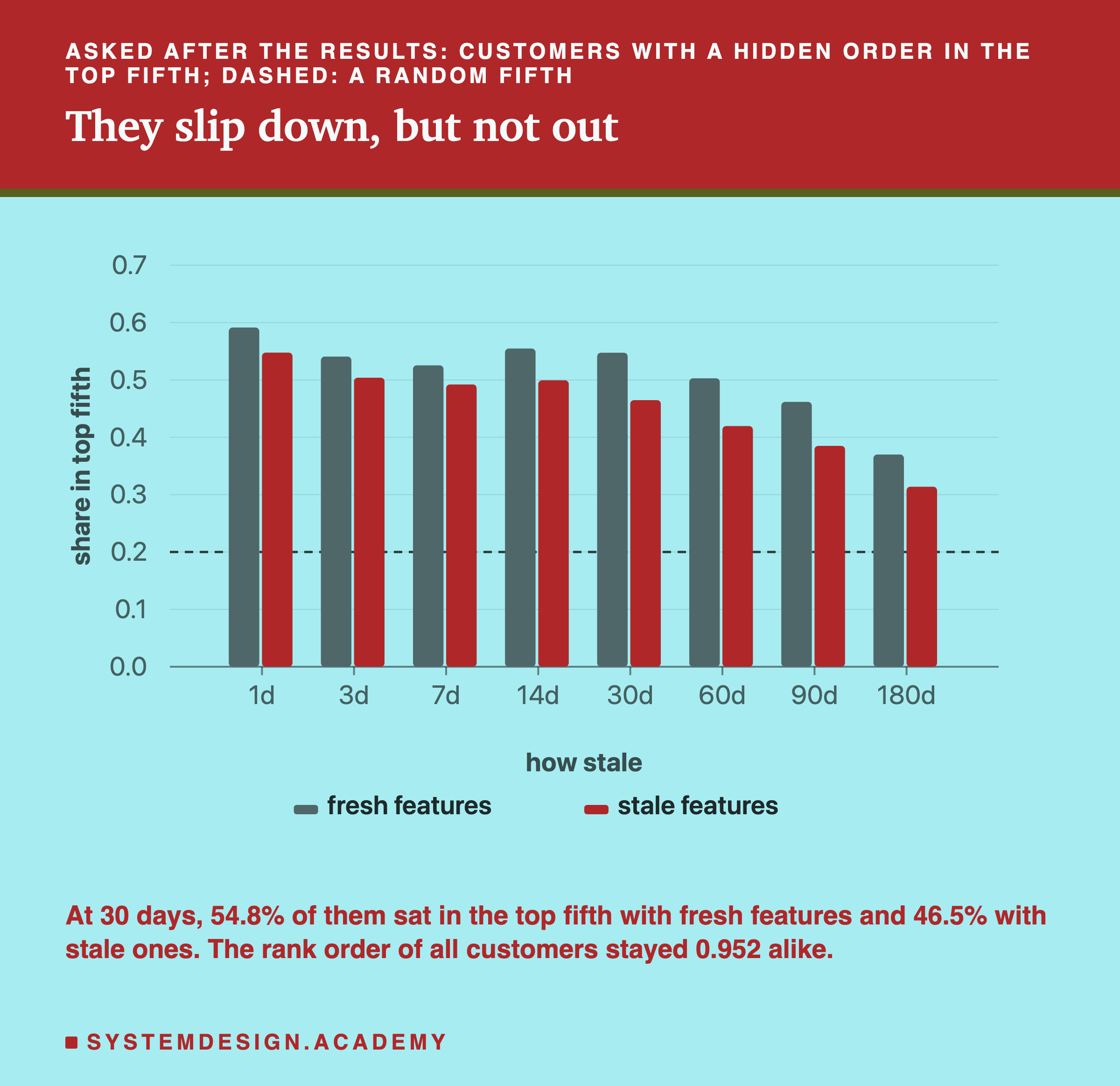
Then I followed the customers with a hidden order, again with the seed 0 model. With fresh features, 54.8 percent of them were in the top fifth of the ranking. With stale features, nearly half still were: 49.9 percent at 14 days and 46.5 percent at 30 days, against one in five by chance. One possible reason, which I did not test: a customer who ordered last week has often ordered before, so their stale card may already say "regular". Their median number of orders was 7 with fresh features and still 7 with 30-day-stale ones.
If that reason holds, habits in this shop change slowly compared with a 30-day question, and the stale card is a slightly older picture of the same habit.
Where It Starts to Cost: Asked After the Results
If a month costs so little, when does staleness start to hurt? The second follow-up question extended the serve-stale arm to 60, 90 and 180 days, with the same model and the same 20 seeds.
The answer is on the right side of the headline chart, past the dashed line. The cost grows steadily:
| lag | test rows with a hidden order | serve-stale test AP, mean of 20 seeds | change against fresh | 95% interval of the change, 20-seed mean |
|---|---|---|---|---|
| 30 days | 5,461 | 0.5415 | -0.0037 | -0.0088 to +0.0009 |
| 60 days | 8,554 | 0.5280 | -0.0171 | -0.0229 to -0.0116 |
| 90 days | 10,529 | 0.5100 | -0.0352 | -0.0423 to -0.0286 |
| 180 days | 14,386 | 0.4725 | -0.0726 | -0.0813 to -0.0635 |
All 20 seeds were below fresh at every one of these lags. From 60 days on, the interval, which comes from the bootstrap added after the review, also sits clearly below zero. At 180 days, half a year, more than half of the test rows had a hidden order, and the score had lost 0.0726. Even then, 0.4725 is above lesson 1's model on the raw last line, 0.393. Old history still beat no history.
The Repair That Made It Worse
Back to the main run. Here is how the three arms compared at every lag, as the design planned them.
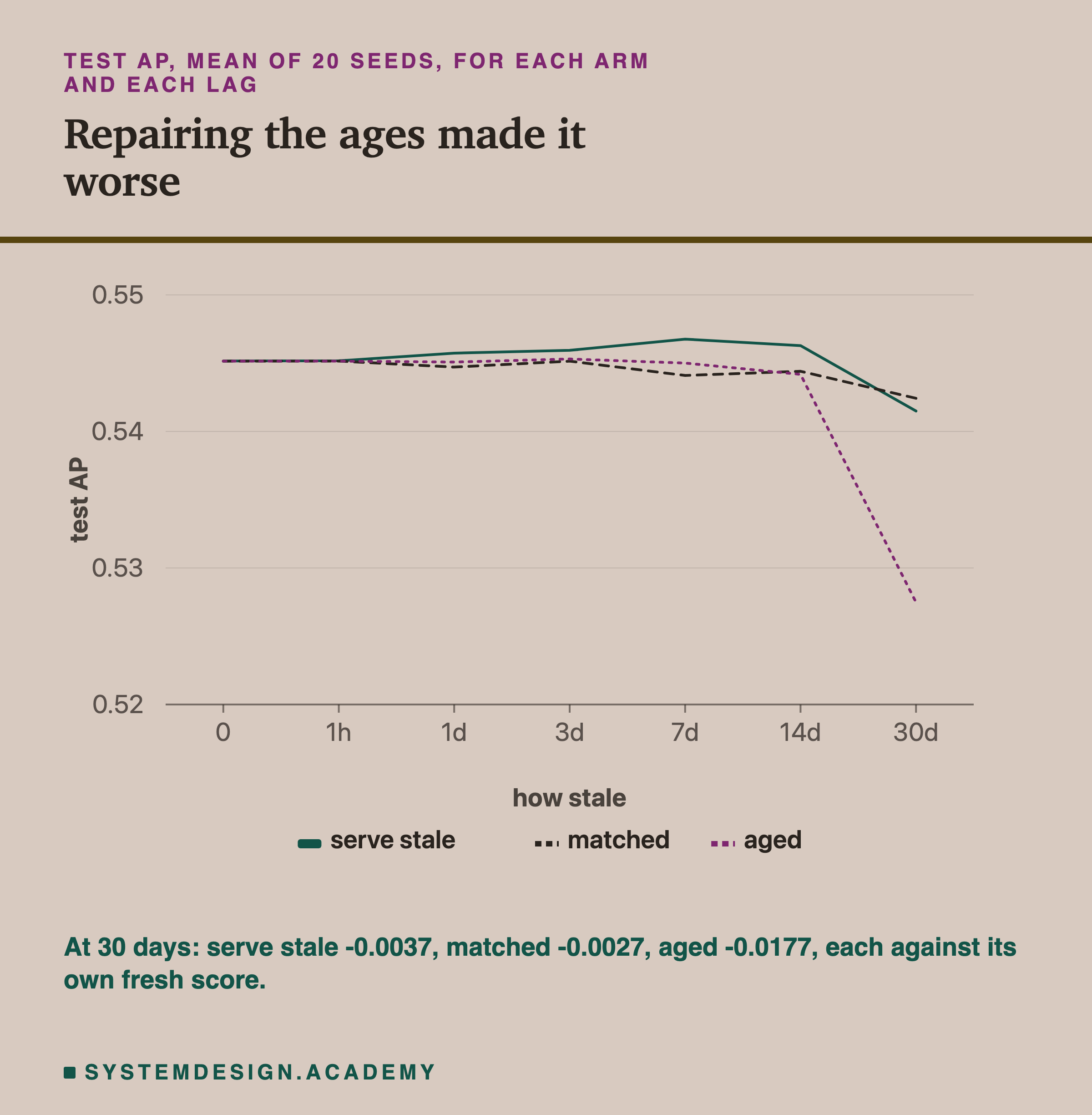
Matched, training on rows with the same lag, did not clearly help. At 30 days it cost 0.0027 against serve stale's 0.0037, and the bootstrap of its 20-seed mean, -0.0078 to +0.0021, included zero. My guess that matching would cost less at every lag was wrong: at 7 days, matched was 0.0011 below fresh while serve stale was 0.0016 above. The two arms cannot be told apart here.
Aged was the surprise. Adding the lag back to the ages cost 0.0177 at 30 days, nearly five times as much as doing nothing, and all 20 seeds were below fresh. The bootstrap of the 20-seed mean ran from -0.0242 to -0.0113, clear of zero. At 14 days aged cost only 0.0010, but 19 of the 20 seeds were below fresh. My guess was the opposite.
Why did a repair hurt? An independent review of my draft asked that, and I checked its answer with a new count, added after the review.
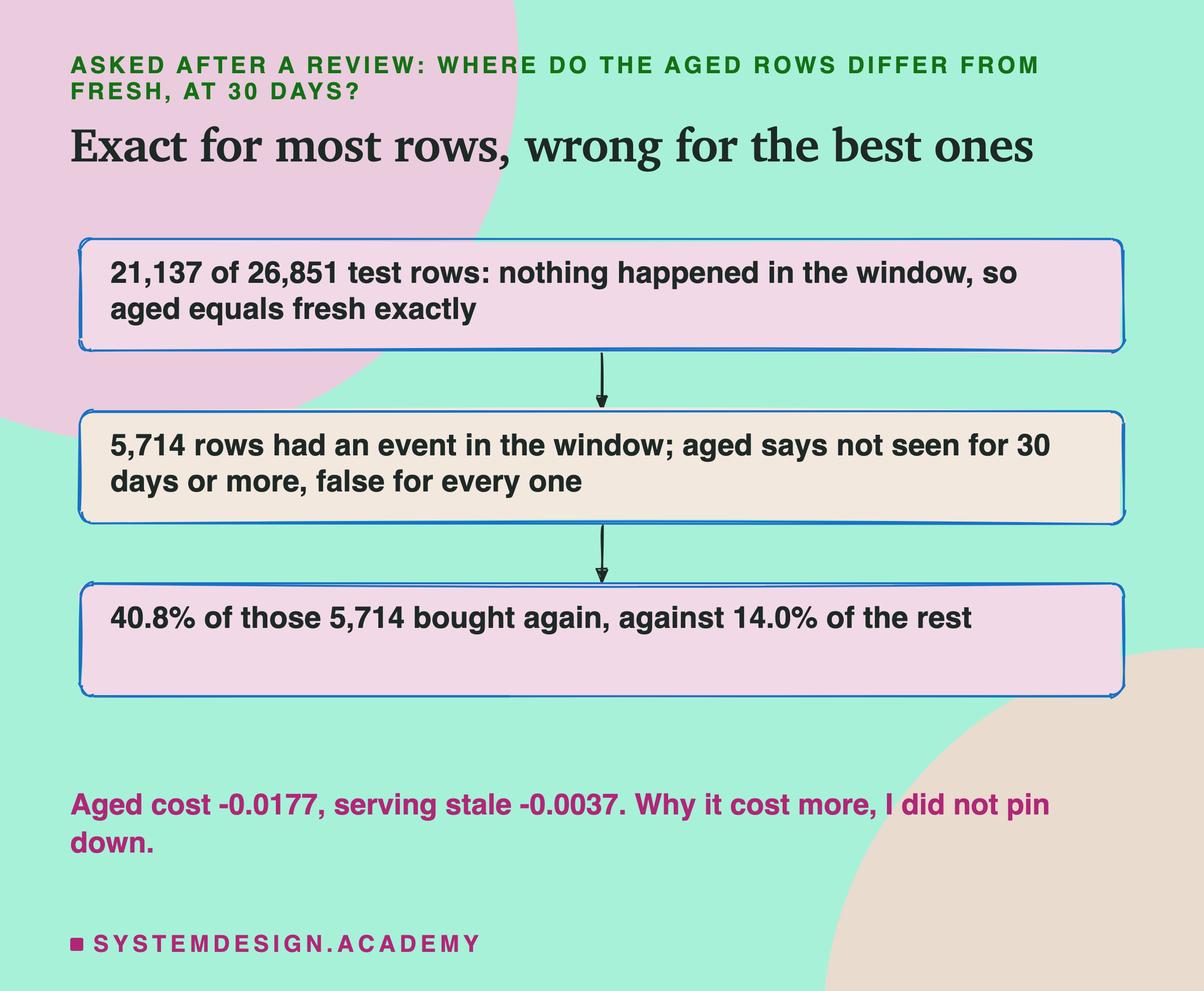
For a customer who did nothing in the 30-day window, adding the lag back is exact. Their last visit and first visit are the same as before, so their ages measured to the cutoff are simply the stale ages plus 30 days. The count agrees: on 21,137 of the 26,851 test rows, all six aged features equal the fresh ones.
The other 5,714 rows had an event inside the window. These are exactly the fresh rows with recency under 30 days, and 40.8 percent of them bought again, against 14.0 percent of the rest. For every one of them the aged row says "not seen for at least 30 days", which is false. So the repair is right for most customers and wrong for exactly the best prospects.
What I could not pin down is why that costs more than serving stale, where those same customers are also wrong. Over the 20 seeds, 46.2 percent of the 5,714 sat in the top fifth with aged rows and 46.4 percent with stale rows, almost the same. The extra loss may come from moves in the order that the top fifth does not show. I did not find them. Lesson 2's rule, work out the age at join time, still holds when the stored time is current. On a stale snapshot, here, it hurt.
One Seed Would Have Told a Different Story
One more result deserves its own slide, because it is the mistake I almost made.
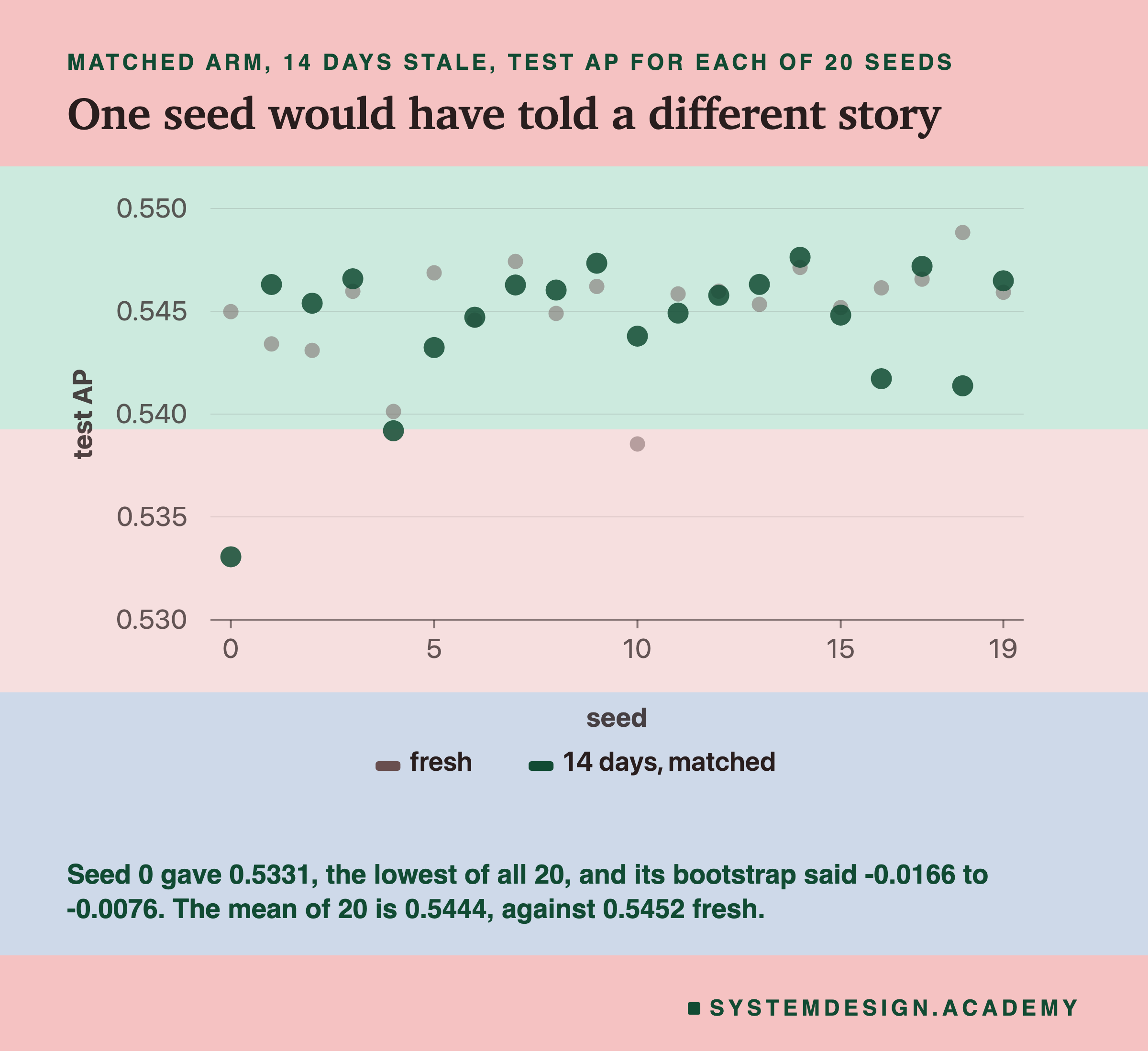
Look at the matched arm at 14 days. With seed 0, it scored 0.5331, against 0.5450 fresh. Its bootstrap interval ran from -0.0166 to -0.0076, nowhere near zero. If I had trained one model, I would have written "training on 14-day-old rows costs 0.012, and the bootstrap proves it".
But seed 0 was the lowest of all 20 seeds. Over the 20, matched at 14 days averaged 0.5444, against 0.5452 fresh, and only 9 of the 20 seeds were below fresh. The low score belonged to one unlucky model, not to the lag.
The bootstrap did not catch this, because it tests the customers, not the training. It takes one trained model as given. This is why every number in this lesson is a mean over 20 seeds, and why the bootstrap comes on top of the seeds, never instead of them.
The Lab's Code, Piece by Piece
The lab is one Python file, scripts/labs/features/feature_freshness.py. It uses the shared file task.py for the data, the cutoffs and the labels, and imports lesson 1's feature code instead of copying it.
stale_features is the heart of it. It calls lesson 1's build_tables with the cutoffs moved back by the lag: cutoffs - lag. That one subtraction makes every feature stale, and recency and tenure come out measured to the moment the job would have run. Then it shifts the cutoff column forward again and joins the features onto the label rows with how="left". A customer with no row before the lag gets empty values, written as NaN, short for "not a number".
Empty features at serving. The model handles NaN by itself. scikit-learn's documentation covers one special case. If a feature had no missing values in training, a missing value at prediction goes to whichever side of each split held more training rows. That applies to the serve-stale arm, whose fresh training table has no empty rows.
aged adds the lag back to recency_days and tenure_days and changes nothing else.
missed counts, for each test cutoff, the customers with a non-return invoice in the window from the cutoff minus the lag up to the cutoff. A non-return invoice is an ordinary order; returns are invoices whose number starts with "C".
draws the test customers again within each cutoff, 1,000 times, with the same draws for every lag and arm, so the comparisons are paired.
Try It Yourself
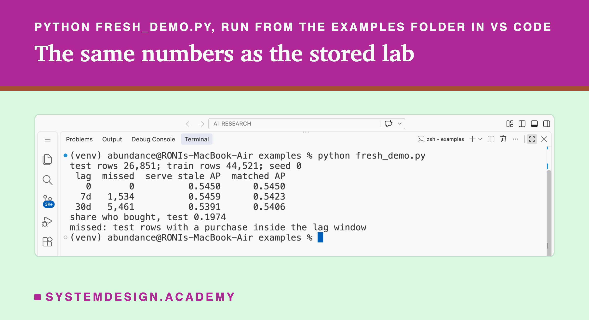
The full lab trains 160 models and takes about 15 minutes. I wrote a small demo that does the heart of it in under a minute: lags 0, 7 and 30 days, serve stale and matched, seed 0.
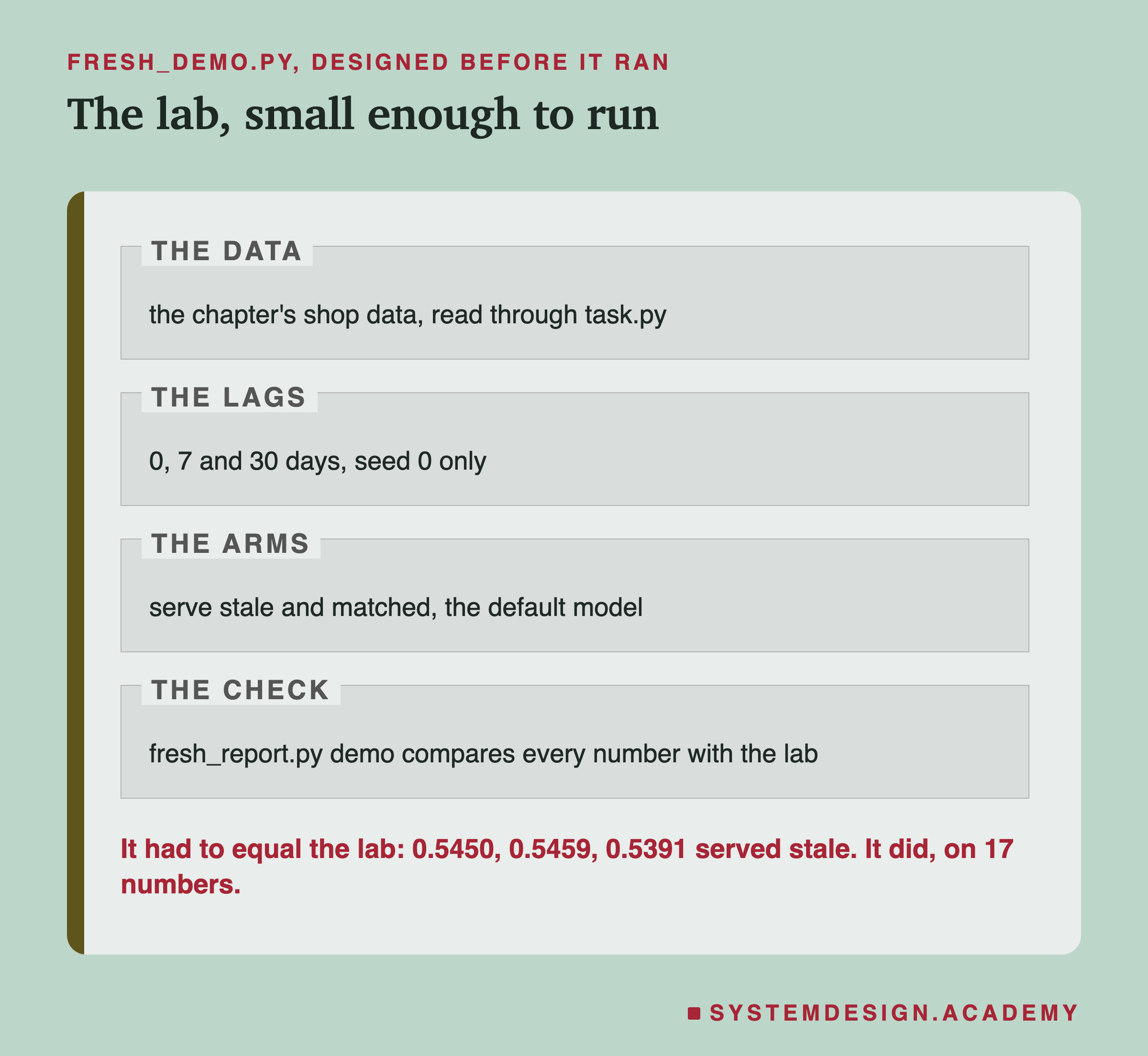
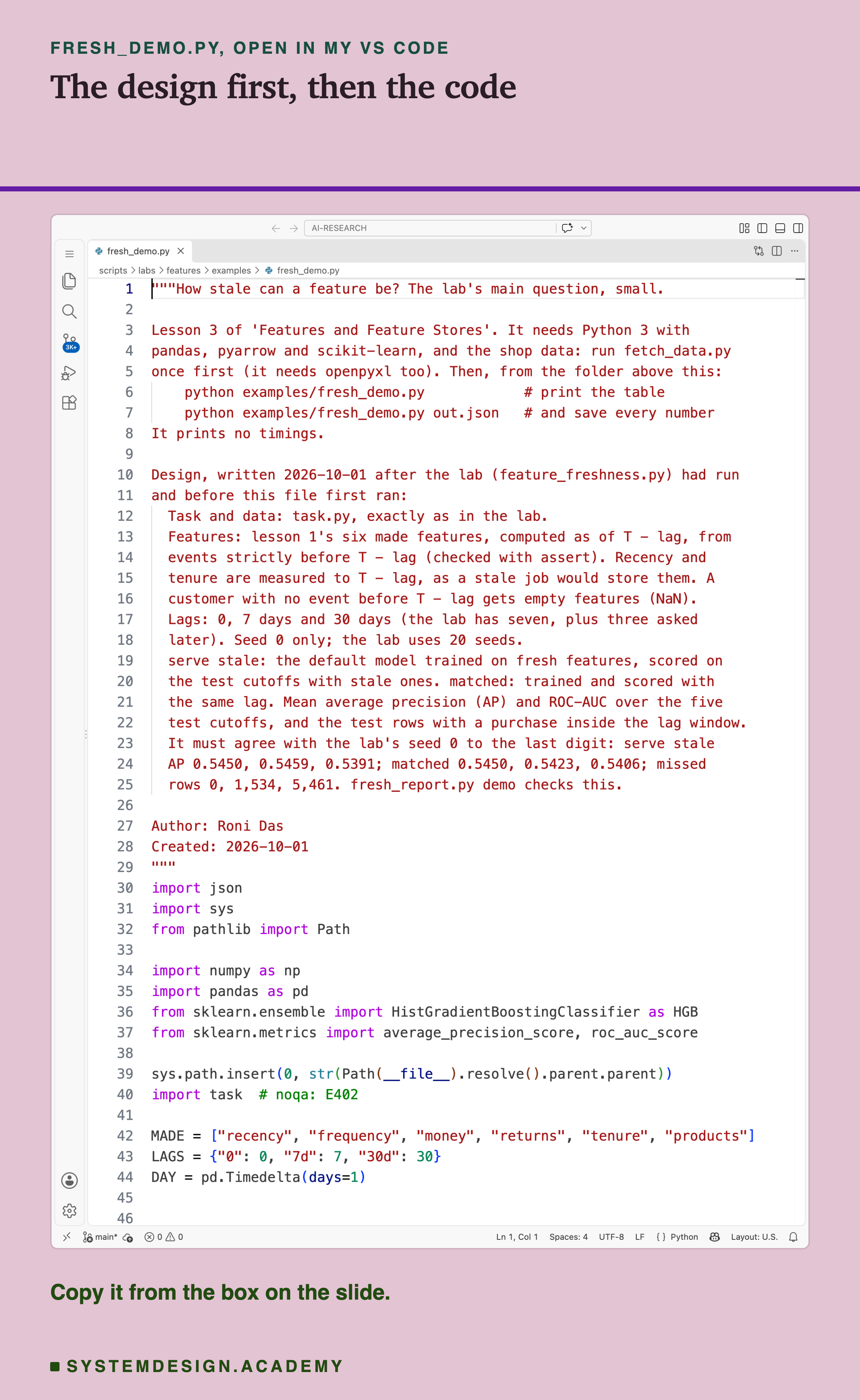
I wrote the demo's design into its docstring after the lab had run and before the demo first ran. It names the numbers it must reproduce: serve stale 0.5450, 0.5459 and 0.5391, matched 0.5450, 0.5423 and 0.5406, and 0, 1,534 and 5,461 rows with a hidden order. It writes its own feature code, about twenty lines, so you can read it in one go.
Before you run this lab. You need Python 3 with pandas, pyarrow and scikit-learn: pip install pandas pyarrow scikit-learn openpyxl. First run python fetch_data.py from the scripts/labs/features folder. It downloads the shop data once, about 46 MB, and writes one cleaned file. Then run the demo from the same folder. On my Mac it took 43 seconds while another program was also running. I ran it with scikit-learn 1.9.1 and pandas 3.0.6 on a Mac. These libraries run on Windows and Linux too, but I have not checked the numbers there. Give it a file name, python examples/fresh_demo.py out.json, and it also saves every number. That is how results/fresh-demo.json was made.
"""How stale can a feature be? The lab's main question, small.

Lesson 3 of 'Features and Feature Stores'. It needs Python 3 with
pandas, pyarrow and scikit-learn, and the shop data: run fetch_data.py
once first (it needs openpyxl too). Then, from the folder above this:
    python examples/fresh_demo.py            # print the table
    python examples/fresh_demo.py out.json   # and save every number
It prints no timings.

Design, written 2026-10-01 after the lab (feature_freshness.py) had run
and before this file first ran:
  Task and data: task.py, exactly as in the lab.
  Features: lesson 1's six made features, computed as of T - lag, from
  events strictly before T - lag (checked with assert). Recency and
  tenure are measured to T - lag, as a stale job would store them. A
  customer with no event before T - lag gets empty features (NaN).
  Lags: 0, 7 days and 30 days (the lab has seven, plus three asked
  later). Seed 0 only; the lab uses 20 seeds.
  serve stale: the default model trained on fresh features, scored on
  the test cutoffs with stale ones. matched: trained and scored with
  the same lag. Mean average precision (AP) and ROC-AUC over the five
  test cutoffs, and the test rows with a purchase inside the lag window.
  It must agree with the lab's seed 0 to the last digit: serve stale
  AP 0.5450, 0.5459, 0.5391; matched 0.5450, 0.5423, 0.5406; missed
  rows 0, 1,534, 5,461. fresh_report.py demo checks this.

Author: Roni Das
Created: 2026-10-01
"""
import json
import sys
from pathlib import Path

import numpy as np
import pandas as pd
from sklearn.ensemble import HistGradientBoostingClassifier as HGB
from sklearn.metrics import average_precision_score, roc_auc_score

sys.path.insert(0, str(Path(__file__).resolve().parent.parent))
import task  # noqa: E402

MADE = ["recency", "frequency", "money", "returns", "tenure", "products"]
LAGS = {"0": 0, "7d": 7, "30d": 30}
DAY = pd.Timedelta(days=1)


def made(ev, labels, cutoffs, lag_days):
    """The label rows at T, with features as of T - lag (NaN if unseen)."""
    out = []
    for t in cutoffs:
        when = t - lag_days * DAY
        past = ev[ev["ts"] < when]
        assert past["ts"].max() < when
        g = past.groupby("customer_id")
        buys = past[~past["is_return"]].groupby("customer_id")
        d = pd.DataFrame(index=g.size().index)
        d["recency"] = (when - g["ts"].max()).dt.total_seconds() / 86400
        d["frequency"] = buys["invoice"].nunique().reindex(d.index).fillna(0)
        d["money"] = g["amount"].sum()
        d["returns"] = g["is_return"].mean()
        d["tenure"] = (when - g["ts"].min()).dt.total_seconds() / 86400
        d["products"] = buys["stock_code"].nunique().reindex(d.index).fillna(0)
        d["cutoff"] = t
        out.append(d.reset_index())
    return labels.merge(pd.concat(out), on=["customer_id", "cutoff"], how="left")


def scores(d, p):
    """Mean AP and ROC-AUC over the five test cutoffs."""
    ap, auc = [], []
    for t in task.TEST_CUTOFFS:
        k = (d["cutoff"] == t).to_numpy()
        ap.append(average_precision_score(d["label"][k], p[k]))
        auc.append(roc_auc_score(d["label"][k], p[k]))
    return {"ap": float(np.mean(ap)), "auc": float(np.mean(auc))}


ev = task.load_events()
lab_tr, _, lab_te = task.splits(ev)
buys = ev[~ev["is_return"]]
fresh = HGB(random_state=0).fit(made(ev, lab_tr, task.TRAIN_CUTOFFS, 0)[MADE], lab_tr["label"])
print(f"test rows {len(lab_te):,}; train rows {len(lab_tr):,}; seed 0")
print(f"{'lag':>4s} {'missed':>7s} {'serve stale AP':>15s} {'matched AP':>11s}")
res = {"rows": {"train": len(lab_tr), "test": len(lab_te)}, "stale": {}, "matched": {}, "missed": {}}
for name, days in LAGS.items():
    te = made(ev, lab_te, task.TEST_CUTOFFS, days)
    hit = set()
    for t in task.TEST_CUTOFFS:
        w = buys[(buys["ts"] >= t - days * DAY) & (buys["ts"] < t)]
        hit |= {(c, t) for c in w["customer_id"].unique()}
    missed = sum((c, t) in hit for c, t in zip(te["customer_id"], te["cutoff"]))
    p = fresh.predict_proba(te[MADE])[:, 1]
    res["stale"][name] = scores(te, p)
    tr = made(ev, lab_tr, task.TRAIN_CUTOFFS, days)
    m = HGB(random_state=0).fit(tr[MADE], tr["label"])
    res["matched"][name] = scores(te, m.predict_proba(te[MADE])[:, 1])
    res["missed"][name] = int(missed)
    print(f"{name:>4s} {missed:7,d} {res['stale'][name]['ap']:15.4f} "
          f"{res['matched'][name]['ap']:11.4f}")
print(f"share who bought, test {lab_te['label'].mean():.4f}")
print("missed: test rows with a purchase inside the lag window")

if len(sys.argv) > 1:
    json.dump(res, open(sys.argv[1], "w"), indent=1)
Make a Card Stale Yourself
This box holds customer 12433's real invoices before 1 November 2011, and the lab's real scores at every lag. It needs nothing but Python, so it runs in your browser. Press Run to see the customer's features fresh and 7 days stale, and which invoices the stale job never saw.
Then change LAG near the top to "30d", "3d" or "180d" and run again. Watch "last seen" jump when an order falls out, then shrink again. The last line prints the lab's mean test AP at that lag, over 20 seeds.
The box computes five of lesson 1's six features. It leaves out products, because that needs every product code on every line. The report script writes this box from the stored lab results. It then runs the box at all nine lags it offers, and checks every printed feature against its own rebuild from the raw lines.
Common Mistakes, and When Freshness Matters
Paying for freshness before measuring it. A streaming pipeline that updates features within seconds is far more work than a nightly job. On this task, two weeks cost nothing I could measure. Replay your own lag on your own data first.
Repairing one column of a stale row. The aged arm sounded correct and cost nearly five times as much as leaving the row alone. If a row is stale, keep it whole and consistent. Either refresh all of it or none of it.
Believing one seed. Matched at 14 days looked like a clear loss with one seed and was nothing over 20.
Believing agreeing seeds. Serve stale at 7 days beat fresh on all 20 seeds and was still inside the bootstrap's noise. Seeds and the bootstrap check different things. Use both.
Forgetting new customers. A stale table has no row for anyone who arrived after the job ran. Decide what the model gets for them, and test it. A later lesson in this chapter is about exactly that.
When freshness matters a lot. When the thing you predict changes as fast as the lag, or faster. Fraud on a card that was stolen an hour ago, what a user wants to watch next, the price of a ride right now. The signal lives in the last minutes, and a nightly job would miss all of it.
When it matters little. When the question is about slow habits, like this one: will a customer buy within a month, asked once a month. Then a picture of last week is nearly as good as a picture of today.
What This Lab Cannot Tell You
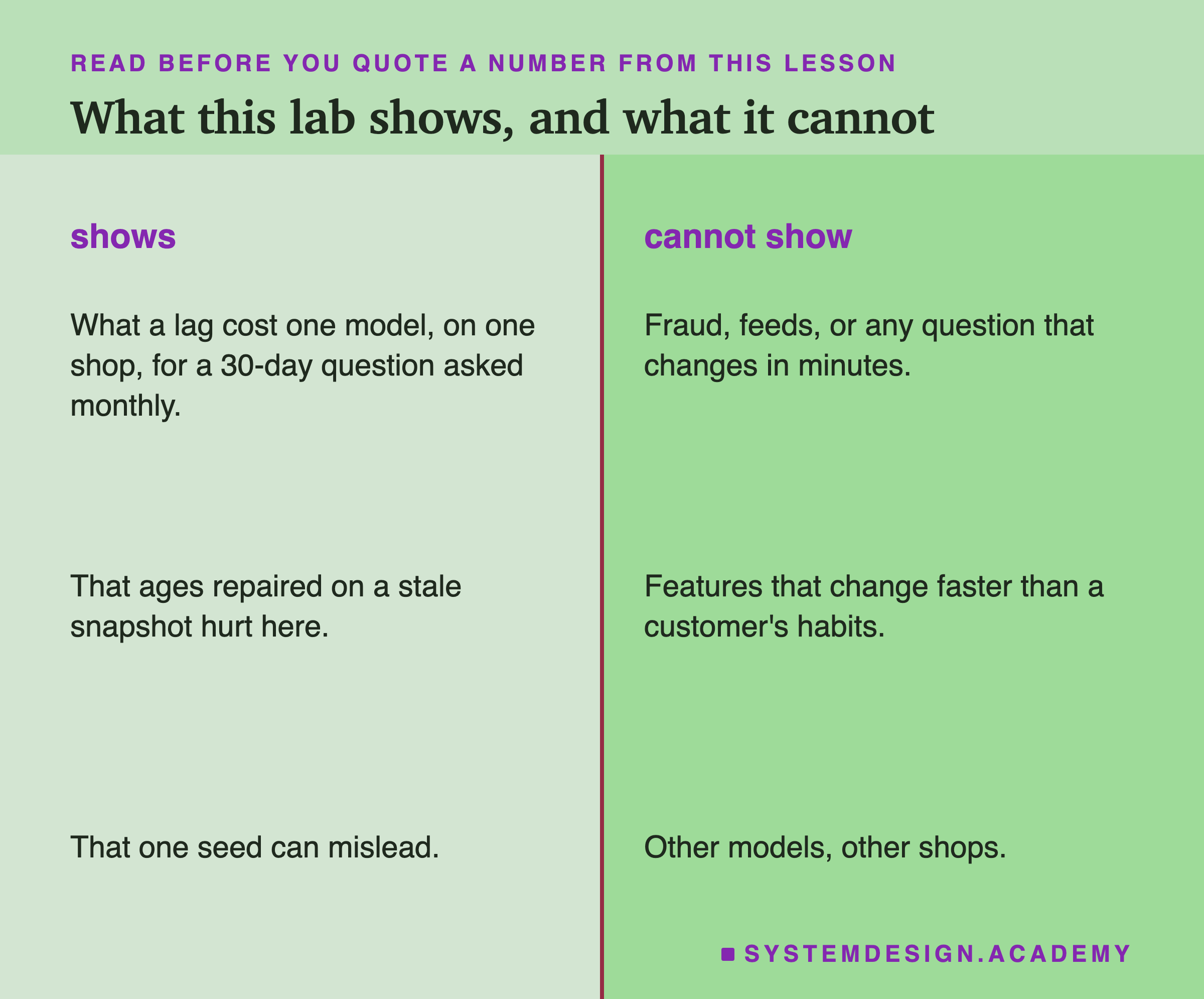
One kind of freshness. The label window is 30 days and the cutoffs are monthly. The features are counts and ages over two years of history. That is a slow question asked about slow features, and it measures one kind of freshness only. I would not use these numbers for fraud scores or real-time systems.
What would differ in a fast system. In a fraud model, the label might be "is this payment fraud", which often arrives weeks later, when the card owner disputes the charge. The useful features are things like "payments from this card in the last ten minutes". A lag of one hour could hide the whole attack. The cost could show up at lags this lab calls free, and the curve could bend in minutes, not weeks. A feed or a recommender has the same shape. To know, you would have to run the same replay with that system's features and labels.
A clean lag. In the lab every customer's features are exactly the same age. A real job finishes at different times for different customers, sometimes fails, and sometimes runs late. That makes the real lag a spread, not one number.
One model. All numbers come from one default gradient boosting model. Another model could react differently to stale values, especially to the empty rows of new customers.
The follow-ups came after the results. The rank, longer-lag and aged questions were asked after I saw the headline, and are labelled so on each slide.
What to Do on Monday
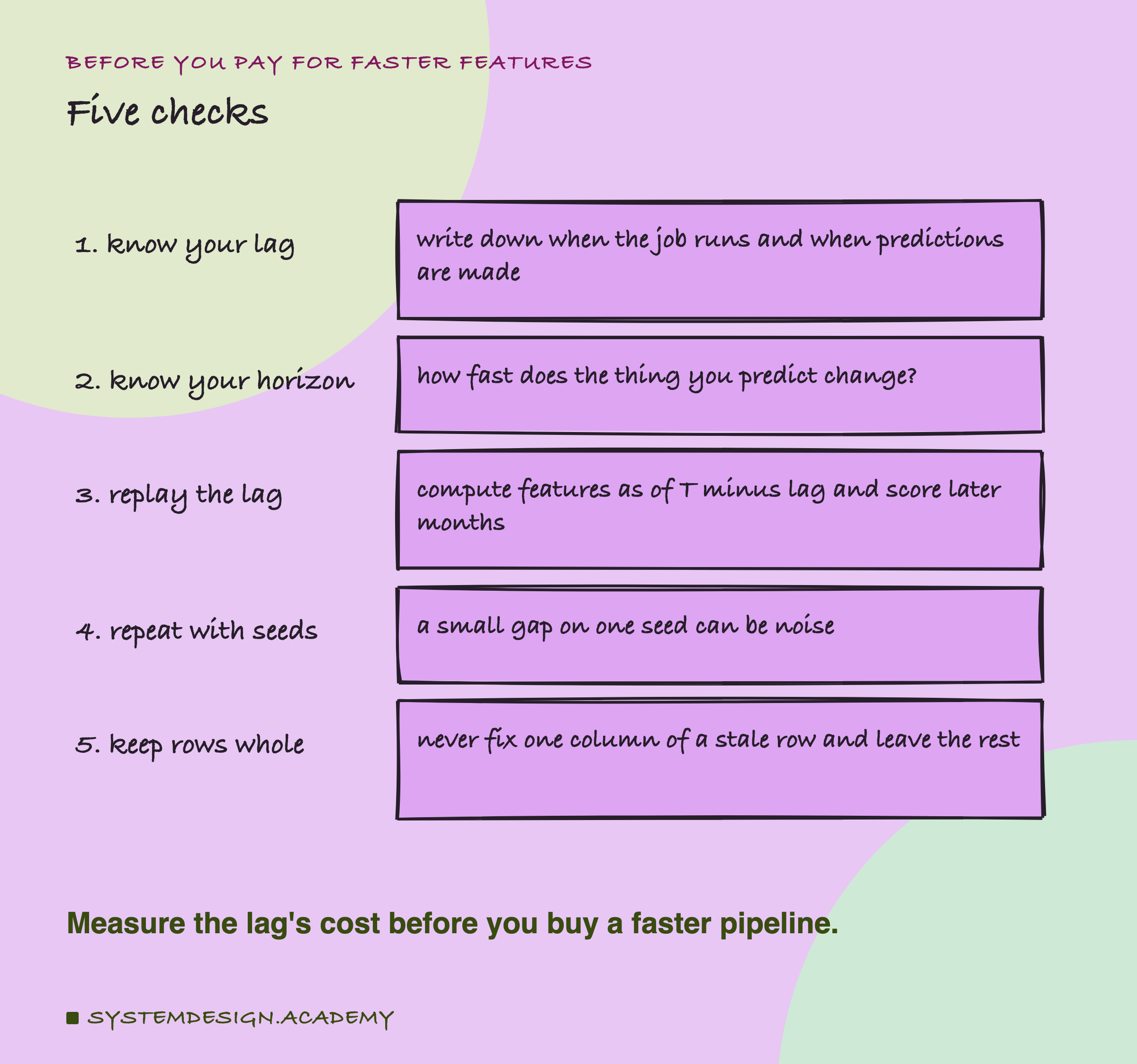
These are the five checks I would make before deciding how fresh a feature pipeline must be.
-
Know your lag. Write down when the job runs, how long it takes, and when predictions are made. The worst-case lag is the gap between runs plus the run time.
-
Know your horizon. How fast does the thing you predict change? A 30-day question about habits and a 10-minute question about fraud need very different answers.
-
Replay the lag. Compute your features as of the cutoff minus the lag, the way this lab does with one subtraction, and score later months. Try several lags, including much longer ones, to see where the curve bends.
-
Repeat with seeds, then bootstrap. A gap that shows up with one seed, or on one set of customers, may be noise.
-
Keep rows whole. Serve a stale row as it was written, or refresh all of it. A half-repaired row can be worse than either.
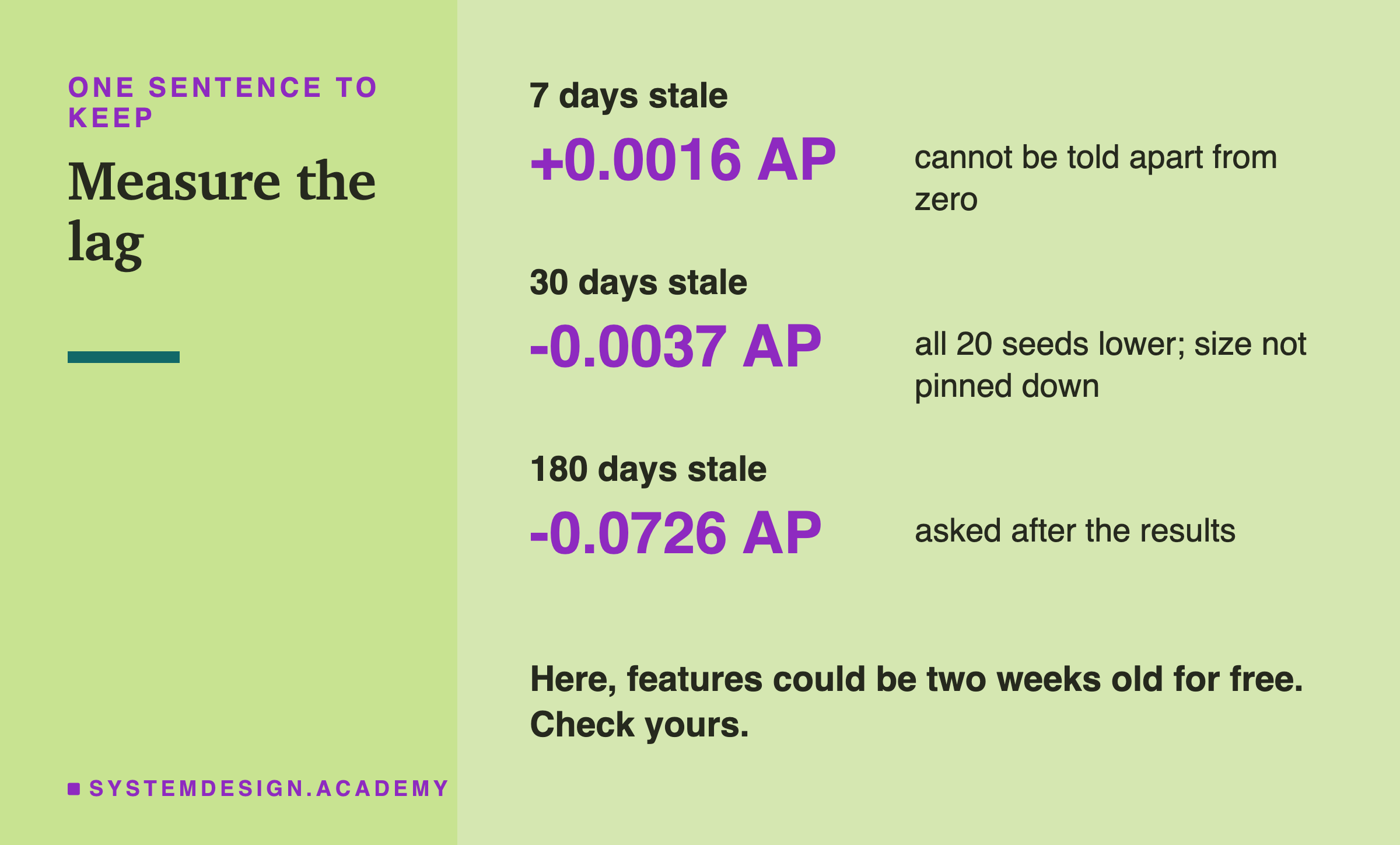
The one idea to keep: freshness has a price and a value, and both can be measured. Here, for a slow question, features two weeks old cost nothing I could measure, and a month cost a little in every seed. Measure yours before you pay for faster ones.
Knowledge Check
Knowledge Check
4 questions - Score 80% to pass
Features served up to 14 days stale changed the mean test AP by an amount the bootstrap could not tell from zero. What is the best reason this lab offers?
The aged arm added the lag back to recency and tenure on a 30-day-stale row. What happened, and why?
With seed 0, the matched arm at 14 days scored 0.5331 and its bootstrap interval did not include zero. Why does the lesson not call that a real cost?
Which system would this lab's result, that two weeks of staleness was free, carry over to the least?