The Paper and the Radio
Imagine two ways to find out about the roads before you drive to work. The first is the morning paper. It is printed once, in the night, from everything the reporters learned during the day before. It is cheap, it is complete, and it is right about yesterday. The second is the traffic report on the radio. Someone reads it out every few minutes, from calls that come in while you listen. It needs people on duty all day and all night, it is never finished, and it can tell you that a bridge closed ten minutes ago.
For some questions the paper is all you need: which roads are usually busy on a Monday, or how long some roadworks will last. For others only the radio will do: is the bridge open right now? Paying a radio station to tell you about next month's roadworks is waste. Reading last night's paper to find out whether the bridge is open right now is no use at all.
A program that learns from examples, which the rest of this course calls a model, has exactly this choice for every number it reads. Take a bank's check on card payments. Here is a made-up example: a card is used in Lagos, and ninety seconds later the same card is used in Toronto.
A program can stop the second payment if it looks at one number: how many times was this card used in the last five minutes? But that number has to be current, this minute. Say it was worked out by a job that ran at 2 AM. Then it still says whatever it said at 2 AM. The payment goes through, and the money is gone. Nothing in the program was wrong. The number it read was old.
Now take a program that guesses which customers will cancel next month, from what they did over the last 90 days. Does it matter whether its numbers are two seconds old or eight hours old? Not at all. Working them out once a night, in one big run, is far cheaper than updating them every time a customer does anything.
Same company, opposite needs. This lesson measures that choice on real data, and the answer turns out to depend less on the program than on each number it reads.
Where This Lesson Starts
This is the first lesson of the chapter on data engineering for ML. Data engineering is the work of getting data from where it is made to the model, in the right shape and at the right time. The first question that work has to answer is when each number is computed.
Two earlier lessons touch this from other sides. In the chapter on why production breaks, train/serve skew sent a model inputs computed a slightly different way at serving time. It used the same hourly bike rentals I use here. In the lifecycle chapter, stale pieces in a pipeline cached one input once a day and measured what the old value cost. This lesson asks the design question that comes before both: which inputs need to be computed fresh at all, and which can be computed once a night?
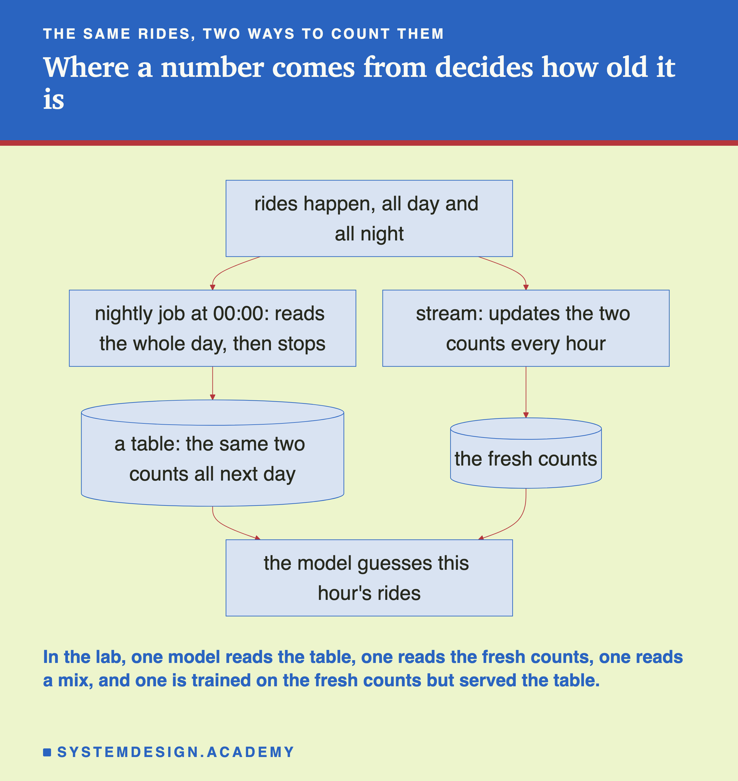
The lesson has two halves. The first is a small lab on real data. One model guesses bike rentals. I serve its two inputs from a nightly job, from a stream, from a mix of the two, and from a job run every few hours. The second half covers the ideas every streaming system is built on, and I explain each one when we reach it. One of them is what a crash does to a count. Where I could, I measured those on the same data. Where I could not, I say so.
Nine Words for This Lesson
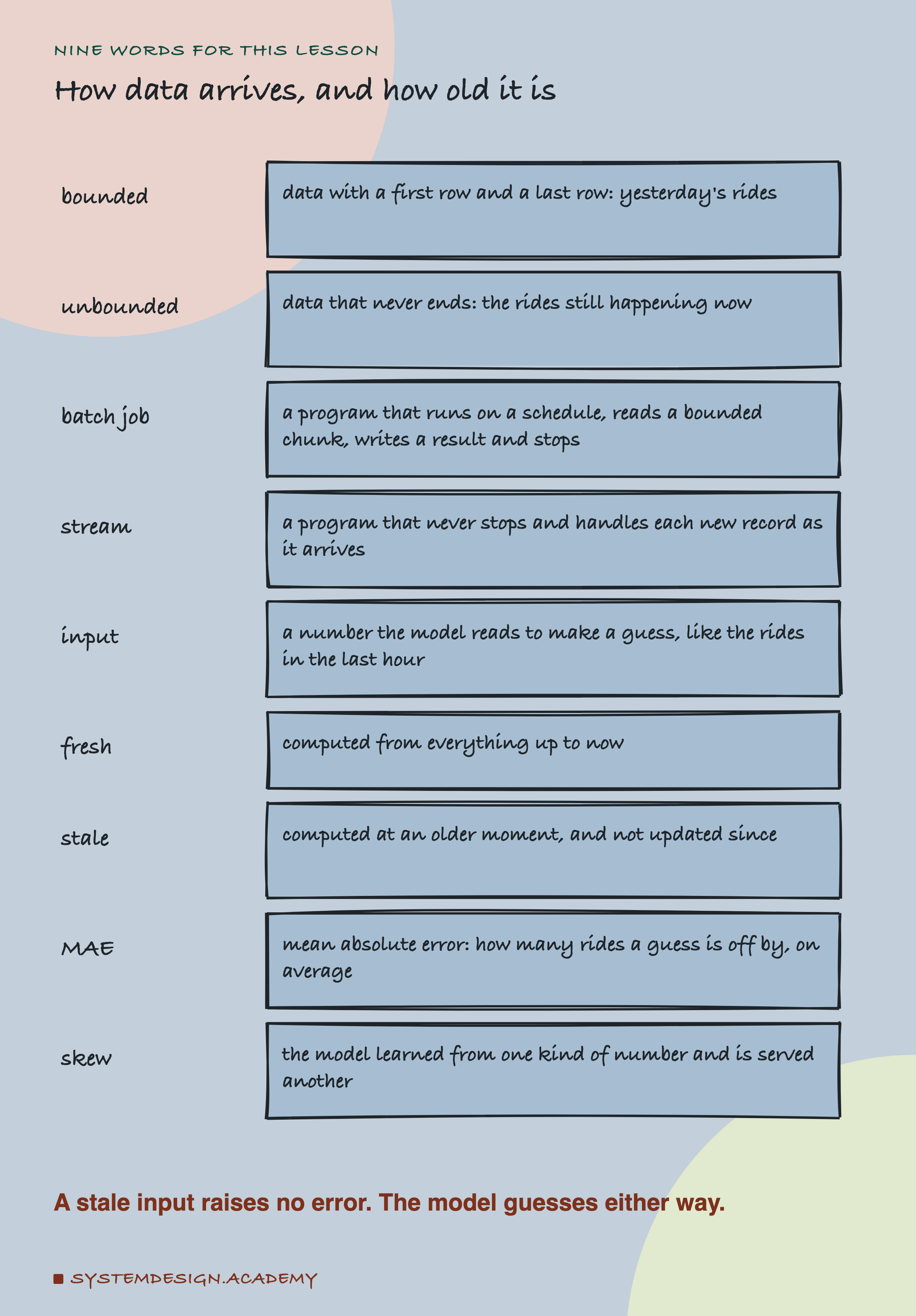
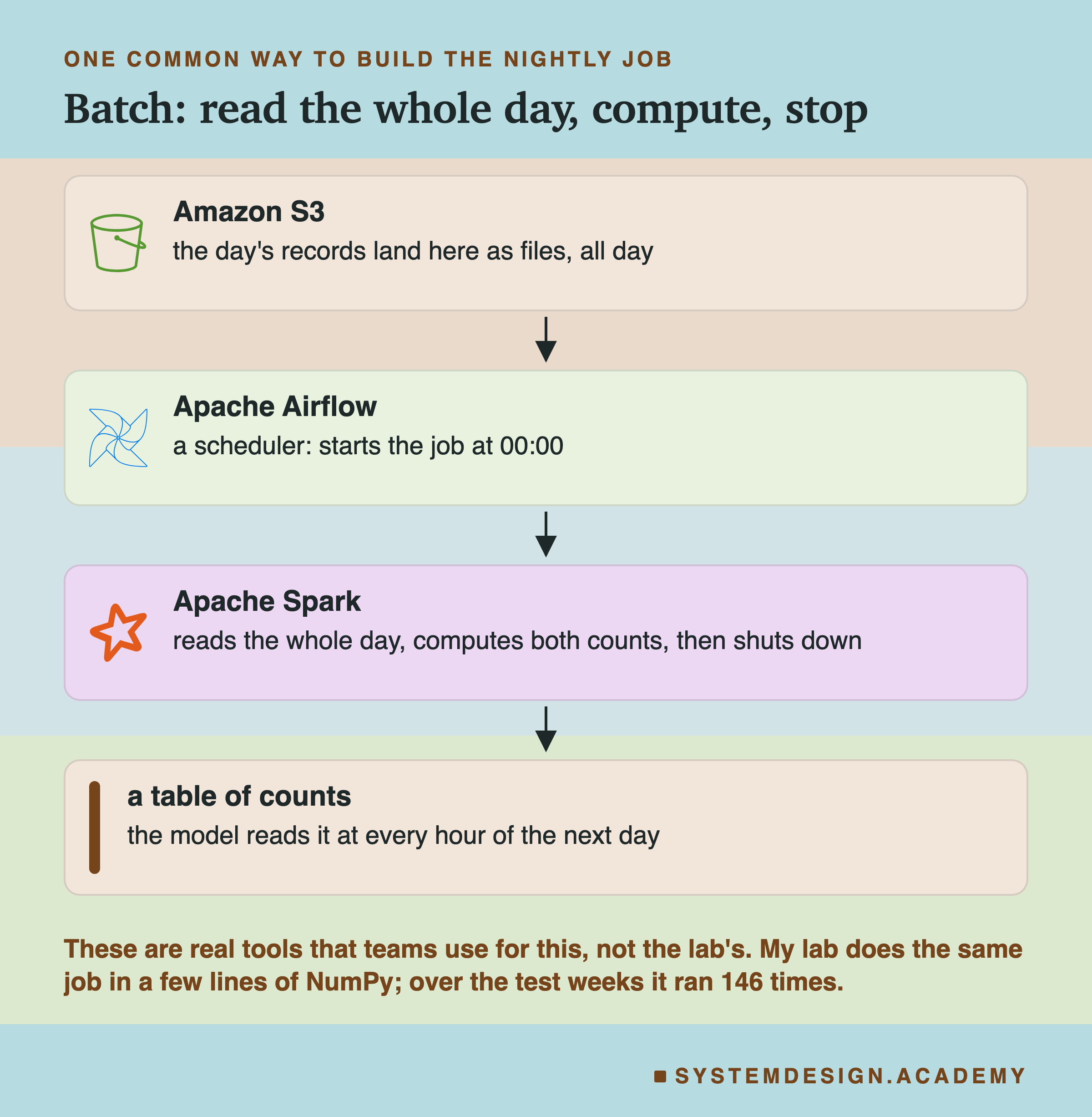
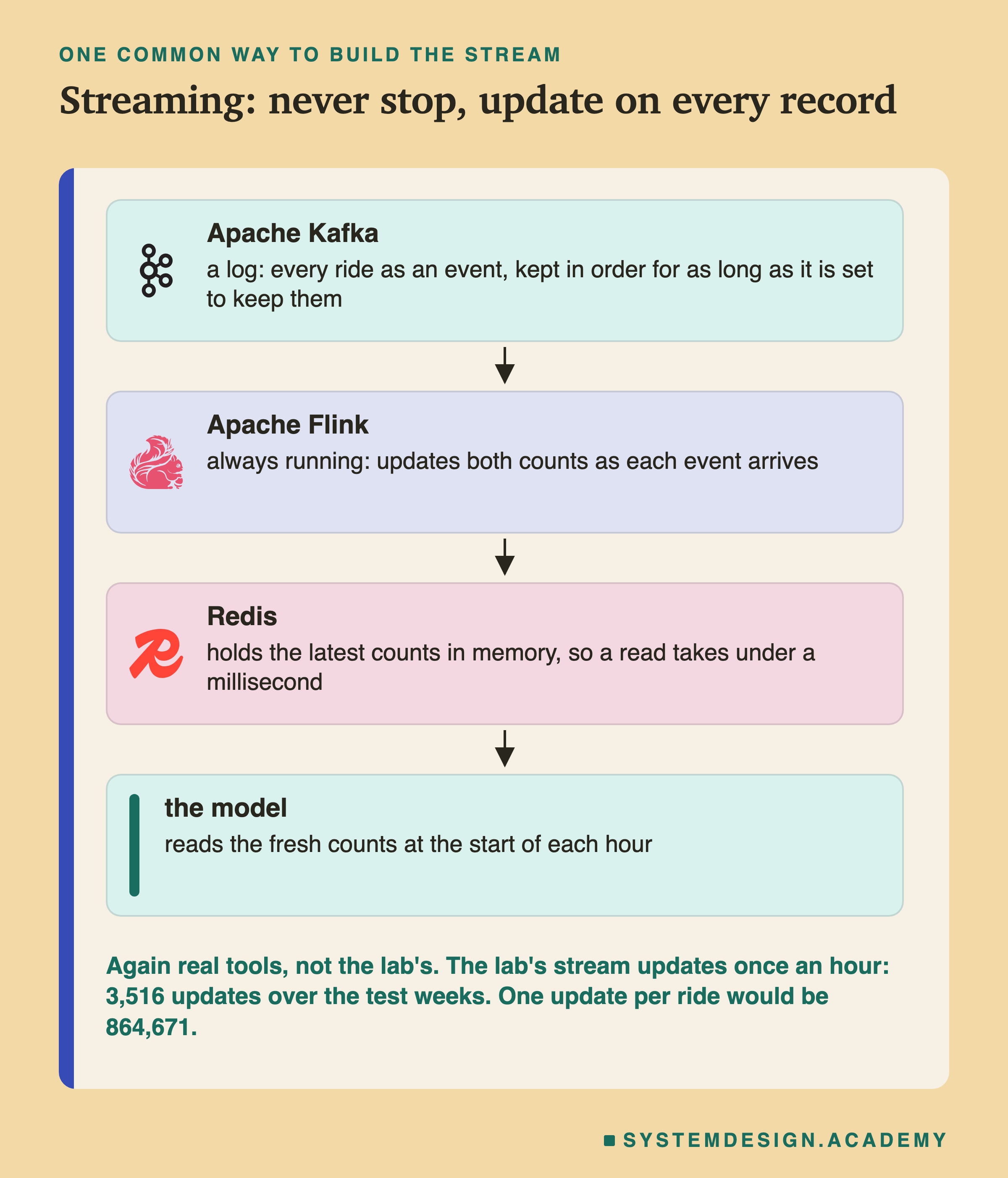
Data is bounded when it has a first row and a last row, like all of yesterday's rides. It is unbounded when it never ends, like the rides still happening now. A batch job is a program that runs on a schedule, reads a bounded chunk, writes a result and stops. A stream, or stream job, is a program that never stops and handles each new record, one row of data, as it arrives.
An input is a number the model reads to make a guess. Many teams call an input a feature; the two words mean the same thing here. An input is fresh when it was computed from everything up to now, and stale when it was computed at an older moment and not updated since. A stale input is not an error. It is a real number of the right type, in the right place. It is just old.
To say how good the guesses are, I use the mean absolute error, MAE. For every hour, take how far the guess was from the real number of rides, then average that over all the hours. An MAE of 30 means the guesses were off by 30 rides an hour on average. Lower is better.
Last, skew, short for train/serve skew: the model learned from one kind of number and is then served another. You will see it cost more than anything else in this lesson.
Bounded vs Unbounded: The Real Difference
Three tools come up again and again in this part of the course. Apache Spark runs batch jobs over many machines at once. Apache Flink runs stream jobs. Apache keeps records in order, in named streams called topics, so that other programs can read them. Strip away the tools, and there is one idea underneath everything. Tyler Akidau's essay "Streaming 101" (O'Reilly, August 2015) suggests two words for it that many engineers now use: bounded and unbounded data. His description of unbounded data is "a type of ever-growing, essentially infinite data set".
A batch job works on bounded data: a chunk with a clear start and a clear end, like all of yesterday's rides sitting in a folder of files. The job reads the chunk, computes something, writes the result and stops. It knows when it is finished, because the data runs out.
A stream works on unbounded data: records that keep arriving, one at a time, with no last row. The job never finishes. It handles each record as it lands, and then waits for the next one.
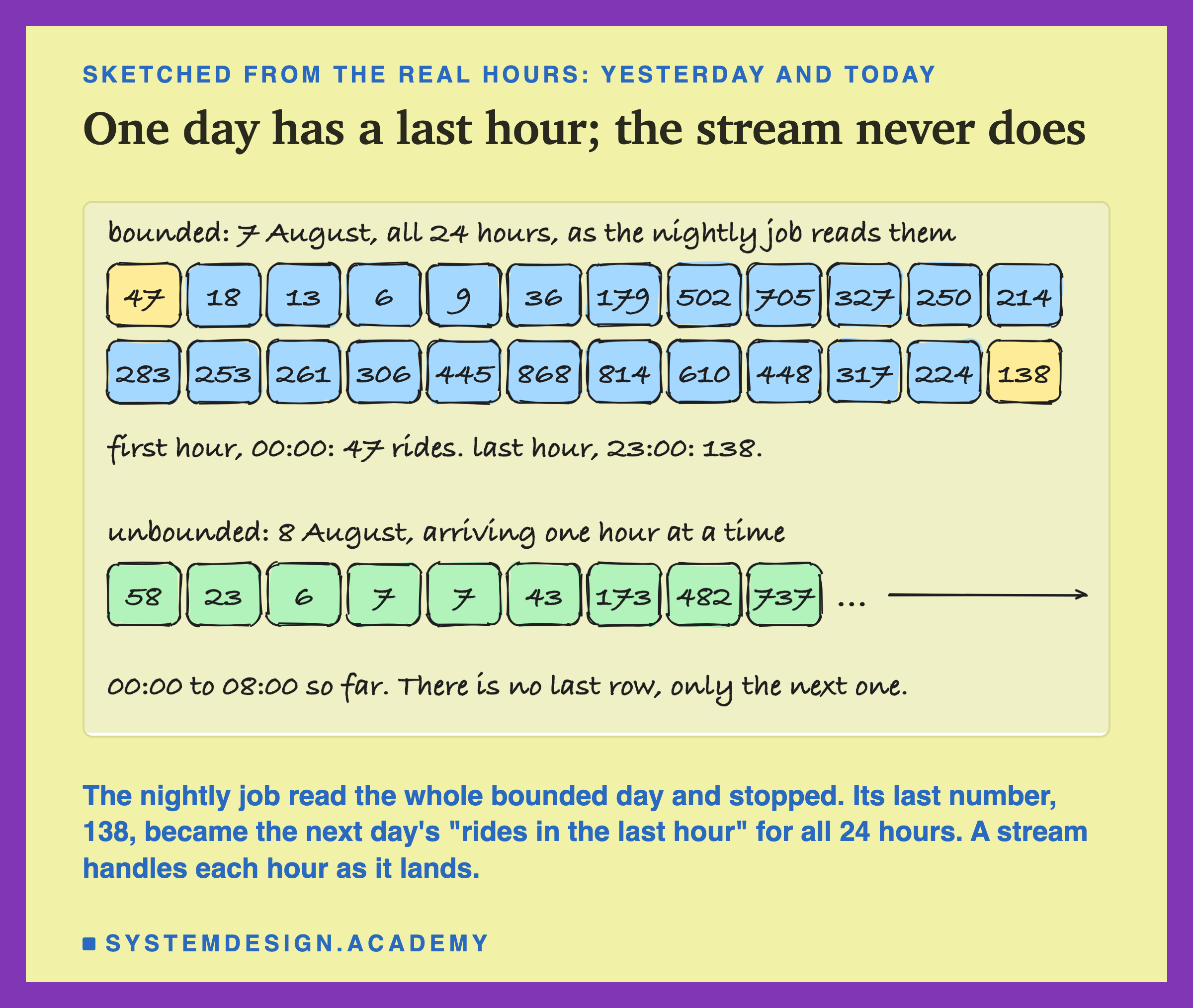
These are two real days from the lab's data. The nightly job reads the whole of 7 August 2012, 24 hours from 47 rides in the first hour to 138 in the last, and stops. The next day is still arriving. Remember that last number, 138. It is what the nightly job hands the model as "rides in the last hour" for every hour of 8 August.
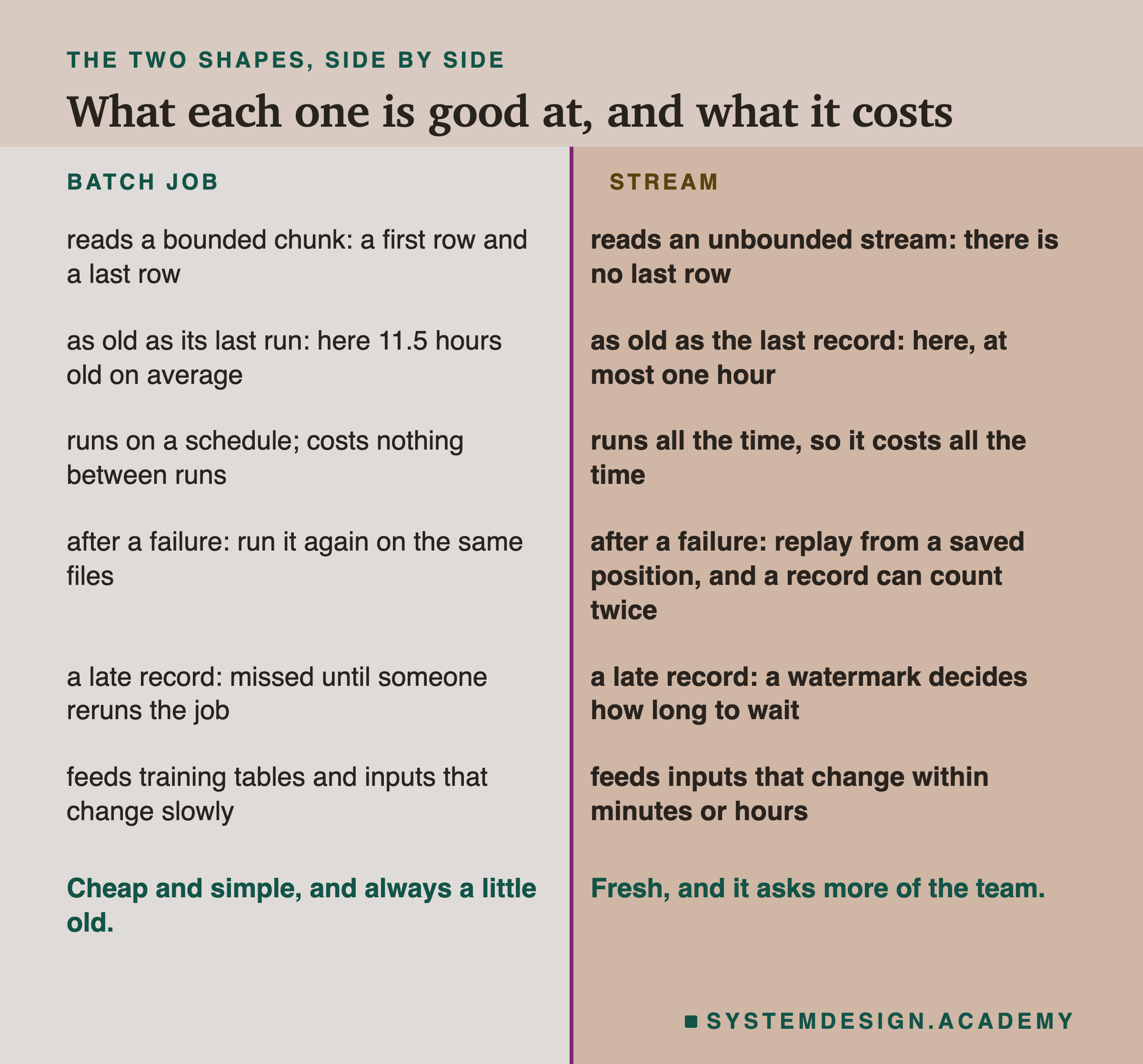
Notice what falls out of the split. Because batch has a fixed chunk, it can be scheduled to run at 00:00. It can work through millions of rows at once. And it costs almost nothing between runs, because nothing is running.
Because a stream has no end, it must run all the time, so it costs all the time. It handles one record at a time. And it has to cope with messy things, like records that arrive late or out of order. Bounded gives you cheap and a little old. Unbounded gives you fresh and more expensive. Every design later in this lesson, Lambda, Kappa, watermarks and delivery guarantees, is a consequence of this one split.
Latency vs Throughput vs Cost
Engineers love to say streaming is better because it is faster. That is not the trade. The real trade has three sides, and you rarely get to win all three. here means how old a result is by the time it is used. means how many rows a system handles for the work it does.
| Side | Batch | Streaming |
|---|---|---|
| Latency | Minutes to hours, set by the schedule | Seconds or less |
| Throughput | Very high, in bulk: one run scans millions of rows at once | Also high on a big enough cluster, but each record is handled on its own, with saved state, so each row takes more work |
| Cost | Low: machines run only on schedule | Higher: machines run all the time, plus saved state |
| Running it | Simple: a job that starts and stops | Hard: late records, records out of order, always on call |
| Doing it again | Easy: run the job again on the old files | Harder: replay the log, or keep a second path |
What the Lab Ran
I wrote the lab's design into the docstring of its script, batch_stream_demo.py, on 30 September 2026, before it ever ran. The script is small on purpose: it is the same file you can copy from this lesson and run yourself.
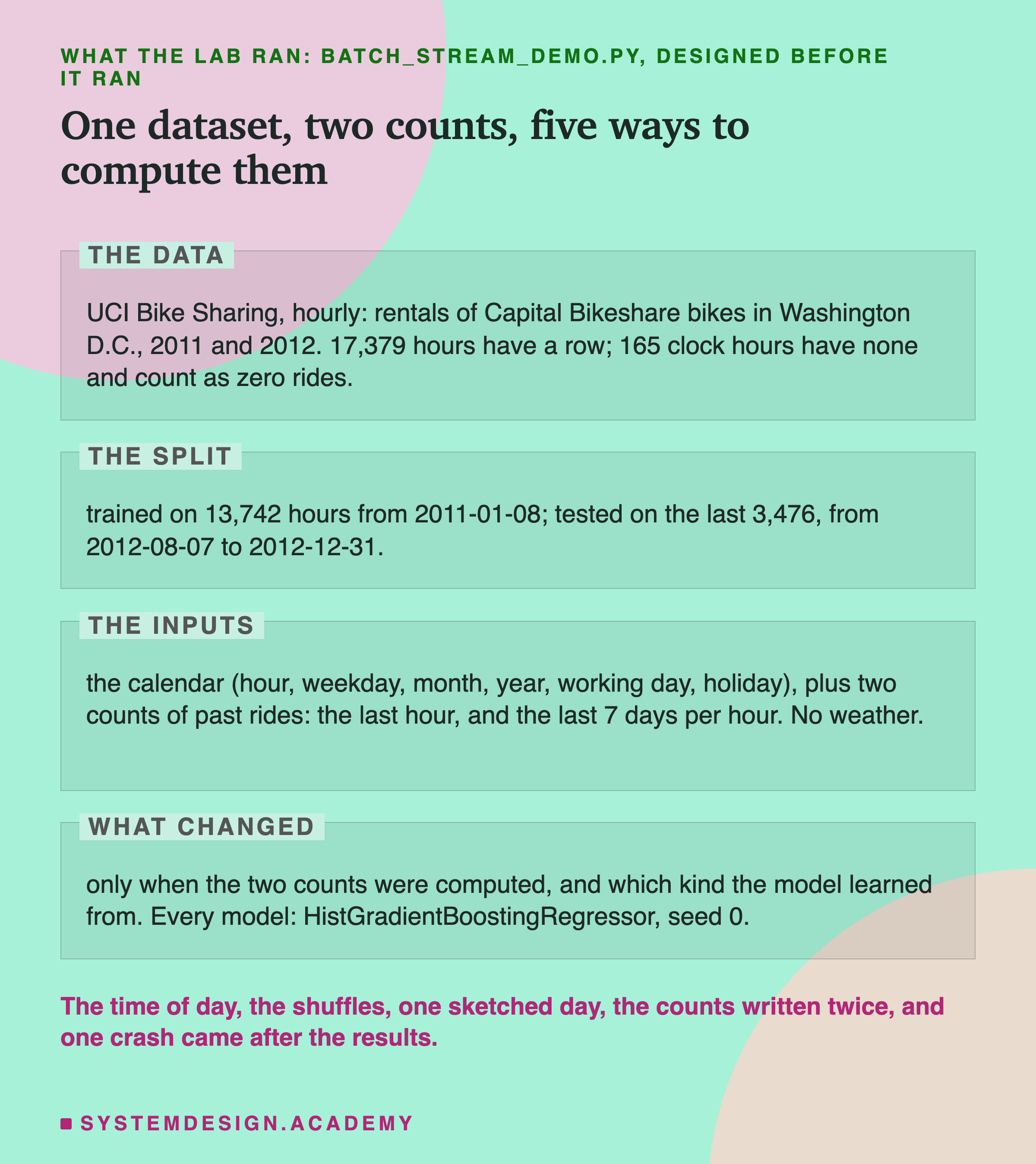
The data is UCI Bike Sharing, the hourly count of bikes rented from Capital Bikeshare in Washington D.C. in 2011 and 2012 (Hadi Fanaee-T and Joao Gama, 2013). It is the same data the chapter on why production breaks used. It has 17,379 rows, one per hour, in time order. The file has the year, the month, the weekday and the hour, but no day of the month. So the script rebuilds the calendar: a new day starts whenever the weekday changes. The report checks the rebuilt date against every row's own year, month and weekday, and every row agrees.
Two full years have 17,544 hours, so 165 clock hours have no row at all. Most of them fall in the small hours of the night. The longest run is 36 hours, from 01:00 on 29 October 2012 to 12:00 on 30 October. That gap matches Capital Bikeshare's shutdown for Hurricane Sandy: a local news site, ARLnow, reported on 31 October that "the system did shut down for about 36 hours". A count of rides is zero when no rides happen. So the script counts an hour with no row as zero rides, and never scores a guess for it.
The task: at the start of each hour, guess how many bikes will be rented in that hour. The model learns from the first 80% of rows: 13,742 hours, starting on 8 January 2011. The first week has no full week behind it, so it is skipped. The model is tested on the last 3,476 hours, from 7 August to 31 December 2012. The real test hours averaged 248.8 rides.
. Every model sees the calendar: the hour, the weekday, the month, the year, and whether the day is a working day or a holiday. I left the weather out on purpose. At the start of an hour nobody knows that hour's weather for sure. And I wanted the only inputs that depend on the pipeline to be two counts of past rides. The is the rides in the last hour, which changes every hour. The is the rides per hour over the last 7 days, 168 hours, which changes slowly.
The Main Run
Here is what the demo stored in results/bv-demo.json.
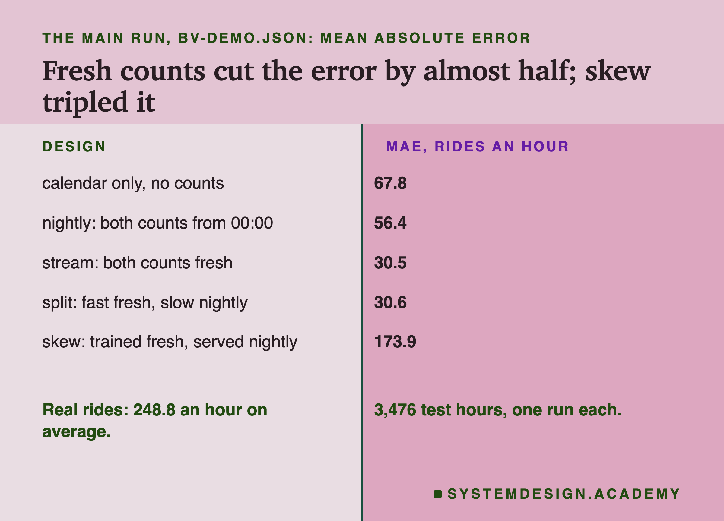
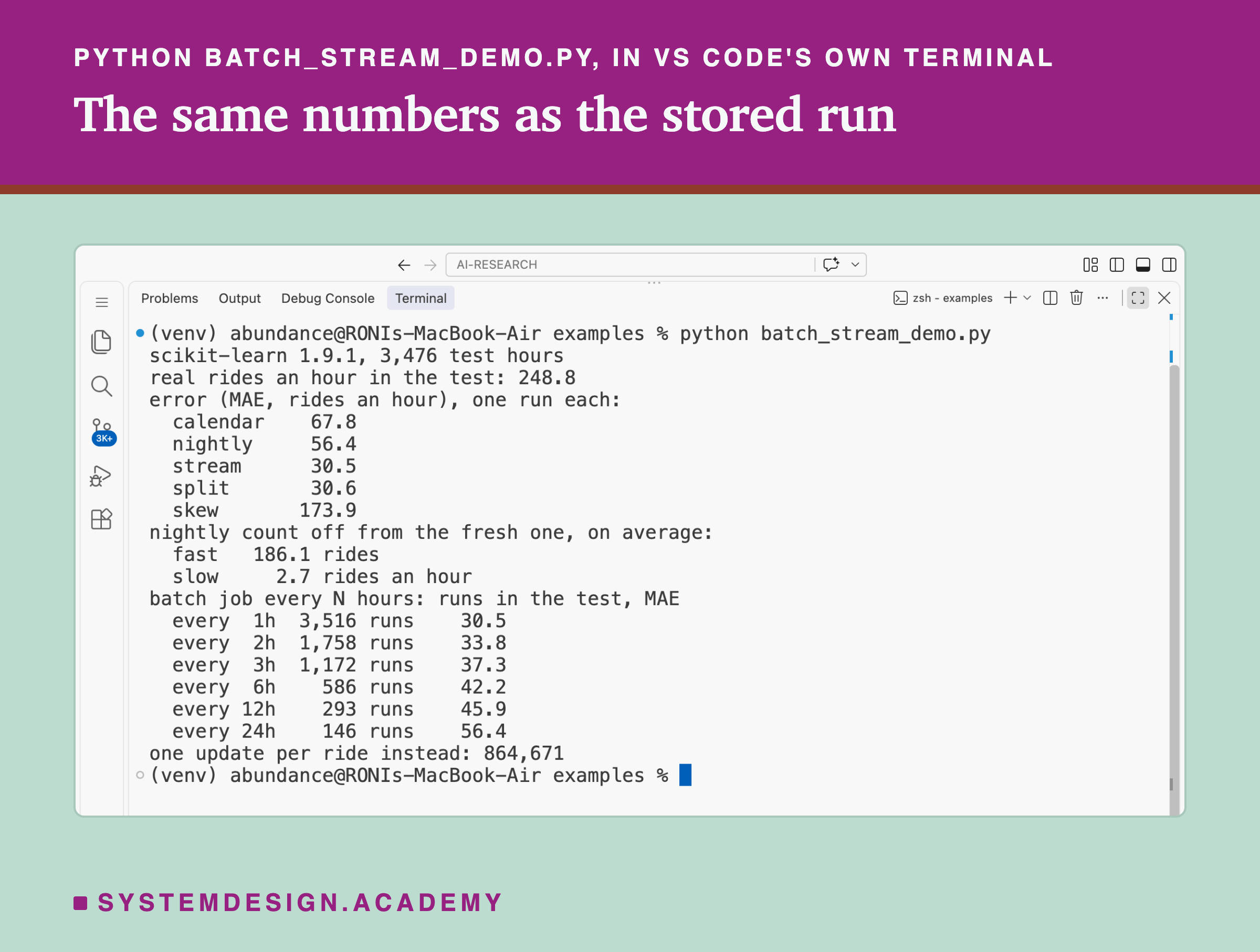
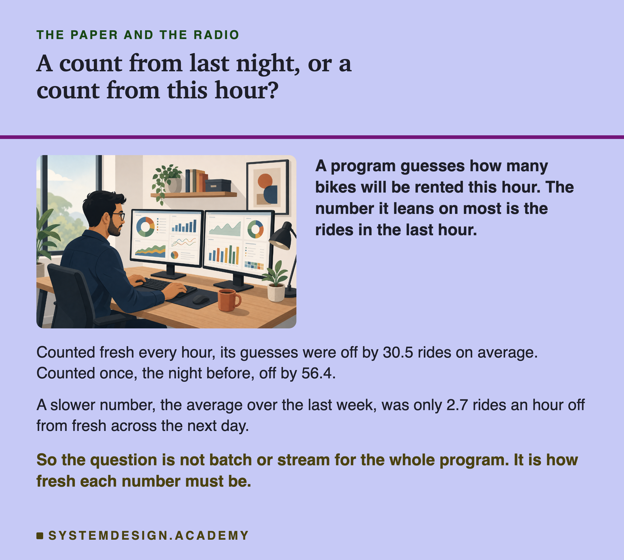
With no counts at all, the calendar alone was off by 67.8 rides an hour on average. Adding both counts from the nightly job brought that down to 56.4. Adding them fresh every hour brought it down to 30.5, so fresh counts cut the error by almost half against the nightly ones.
The split design is the one to look at twice. It took the fast count from the stream and the slow count from the nightly job, and it scored 30.6: 0.09 rides an hour worse than streaming both. The 0.09 itself is too small to read anything into. What matters is the rest of the drop. Streaming only the last-hour count took the nightly design's 56.4 down to 30.6, almost all the way to the 30.5 of streaming both. On this data one count needed a stream and the other did not, so the decision belongs to each input, not to the model.
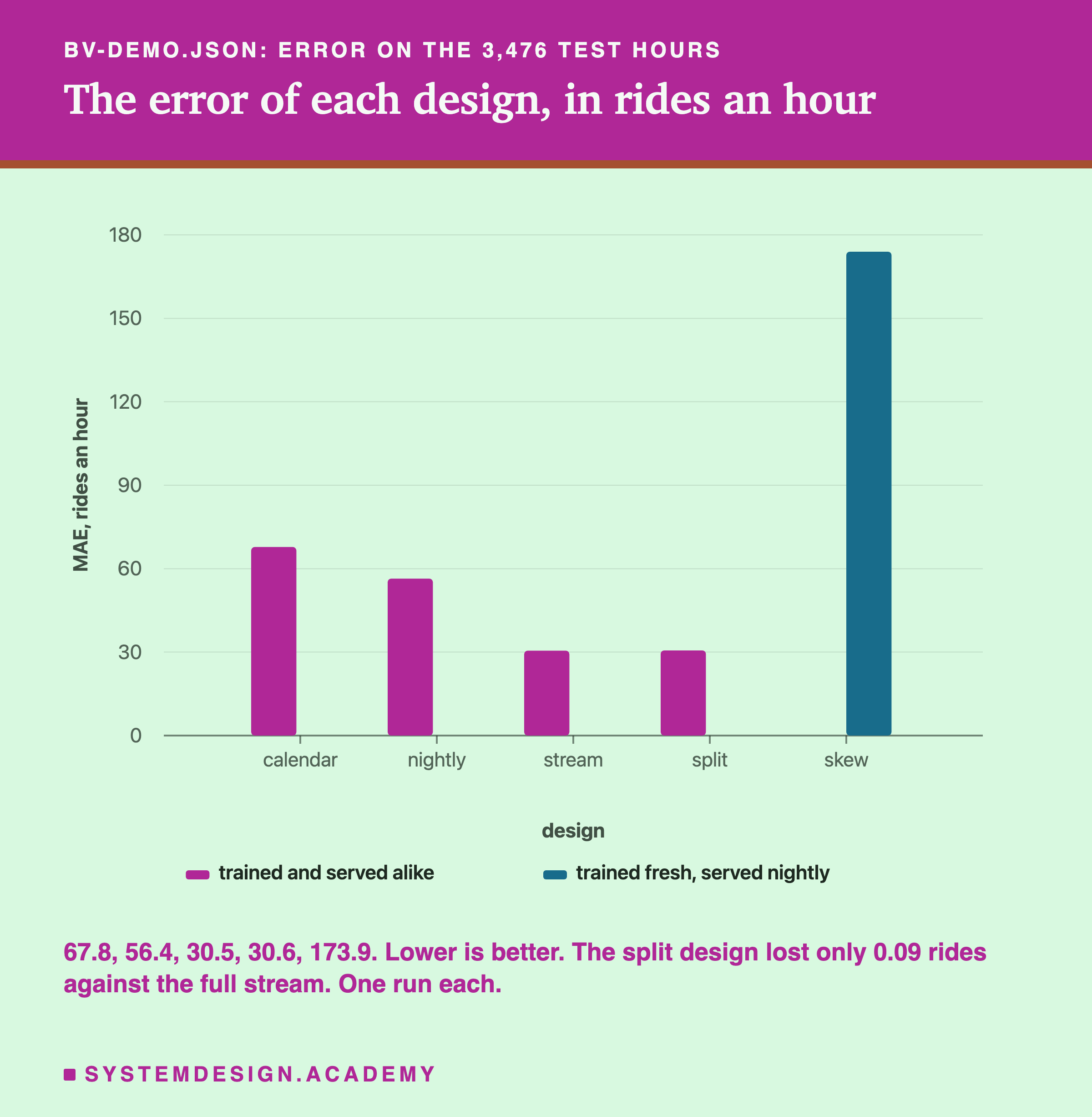
And then skew: 173.9. That model was trained on fresh counts and then served the nightly ones, and it was far worse than knowing nothing but the calendar. The next slides take these numbers apart. Which count needed to be fresh? Where in the day did the difference sit? Why did skew do so much harm? And how often must a batch job run before it gets close to a stream?
Which Count Needed to Be Fresh
Why did one count need a stream and the other not? The simplest measure needs no model at all. On every test hour, compare the count the nightly job served with the fresh count, and average how far apart they are.
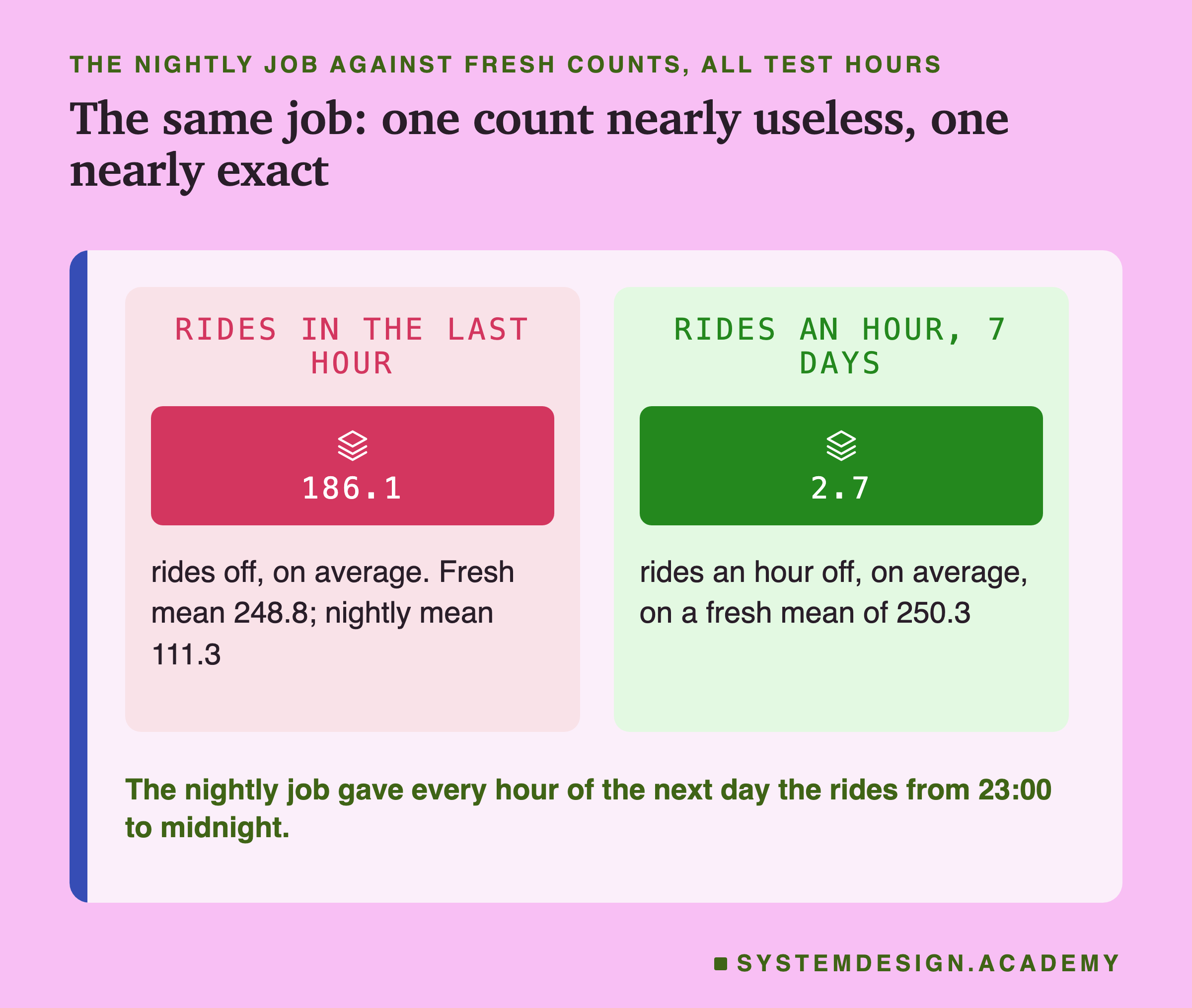
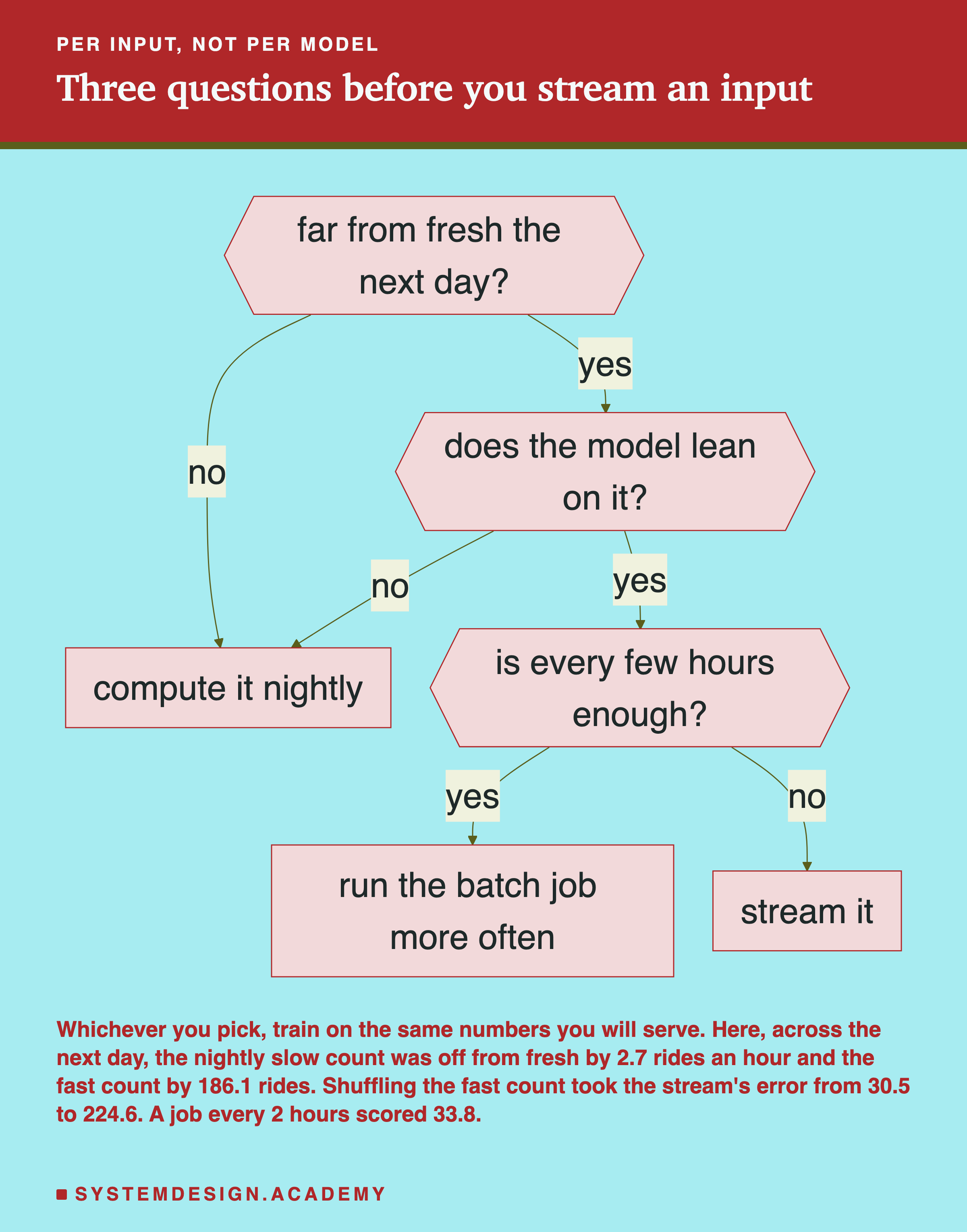
The fast count was off by 186.1 rides on average. The fresh last-hour count averaged 248.8 over the test hours. The nightly one averaged 111.3, because it is always the rides from 23:00 to midnight, a quiet hour. So for every hour of the next day, the nightly job served the number of a late evening. The slow count was off by only 2.7 rides an hour, on a count that averaged 250.3. A week's average barely changes in a day, because most of the hours it covers are the same whether you compute it at midnight or at 18:00.
The nightly values were 11.5 hours old on average when they were used. The job runs at 00:00, so an hour at 23:00 reads a value 23 hours old. But age alone did not decide the damage. What decided it was how much the value changed in that time. So the same age cost the fast count almost everything and the slow count almost nothing.
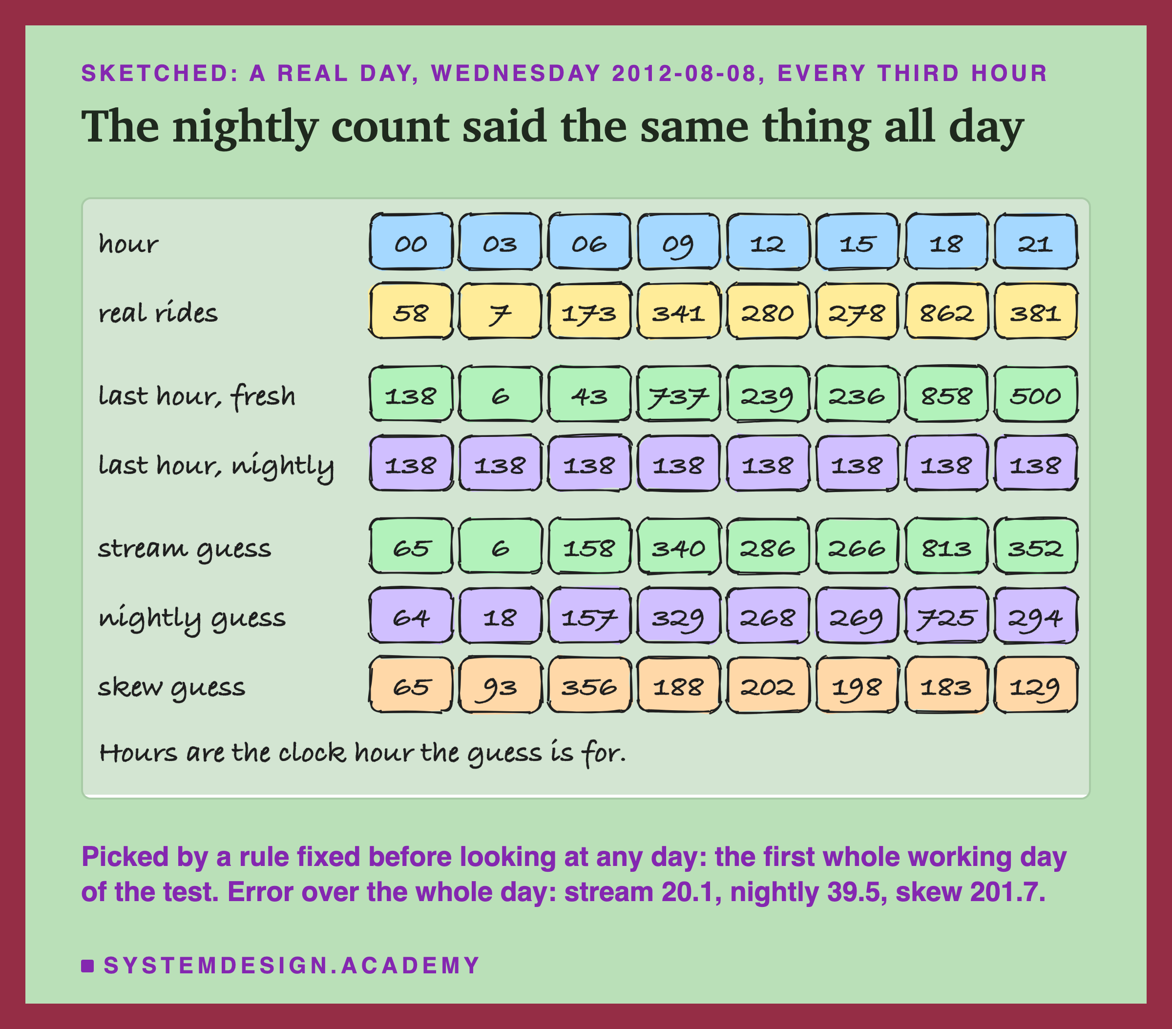
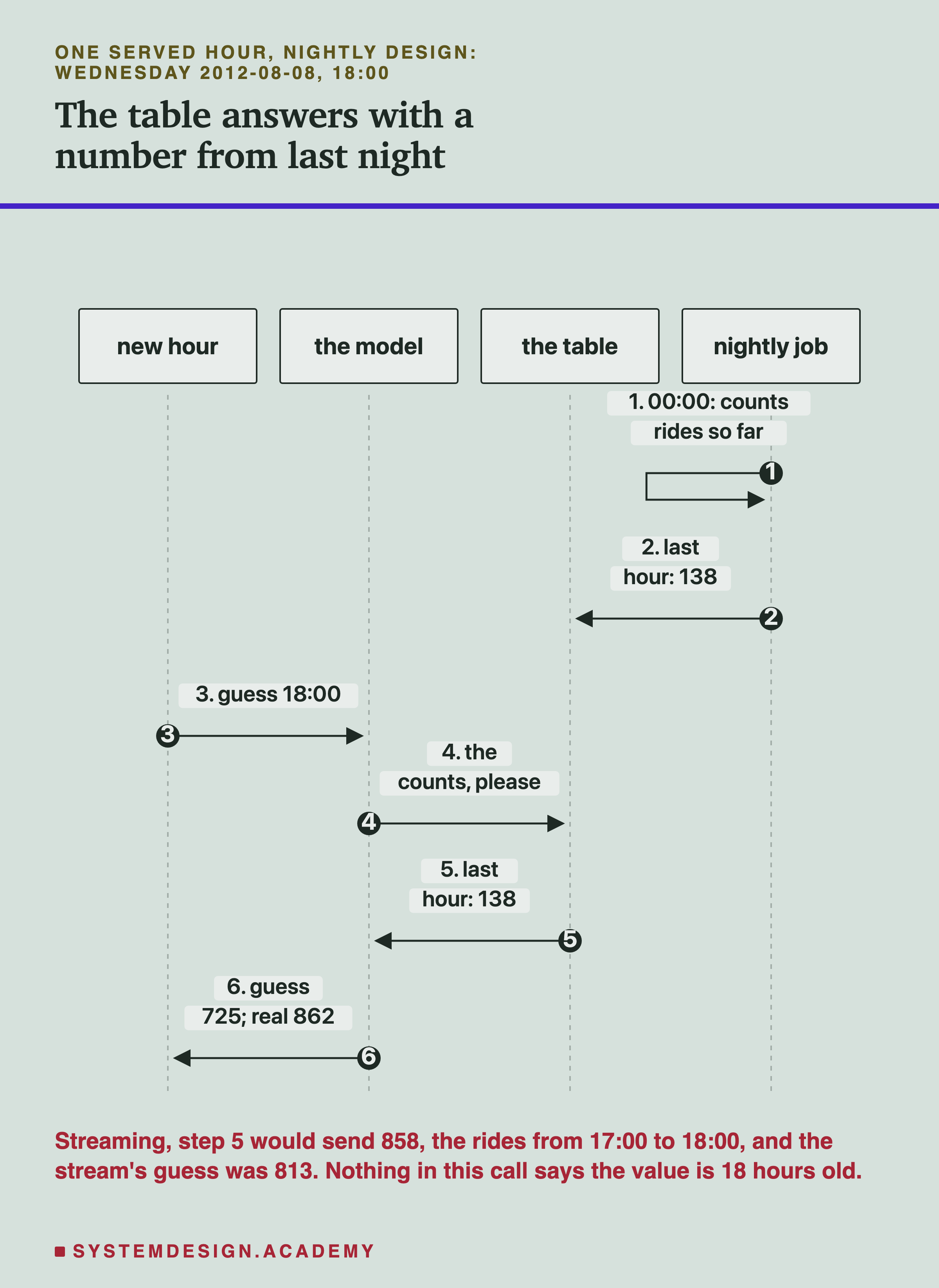
Here is one real day, picked by a rule I fixed before looking at any day's numbers: the first whole working day in the test. At 00:00 the two versions of the fast count agree, 138, because the nightly job has only just run. From then on the nightly count stays at 138. The fresh one follows the day: 6 at 03:00, 737 at 09:00 just after the morning rush, and 858 at 18:00.
The stream's guesses followed the real rides closely. The nightly model's guesses were close in the quiet hours and fell behind in the busy ones: 725 against a real 862 at 18:00. Over the whole day the stream was off by 20.1 rides an hour and the nightly model by 39.5.
Trained Fresh, Served Stale
The skew design was trained on fresh counts and served the nightly ones, and it did worse than no counts at all: 173.9 against the calendar's 67.8. The nightly design was served exactly the same nightly counts and scored 56.4. The only difference between the two is what each one learned from.
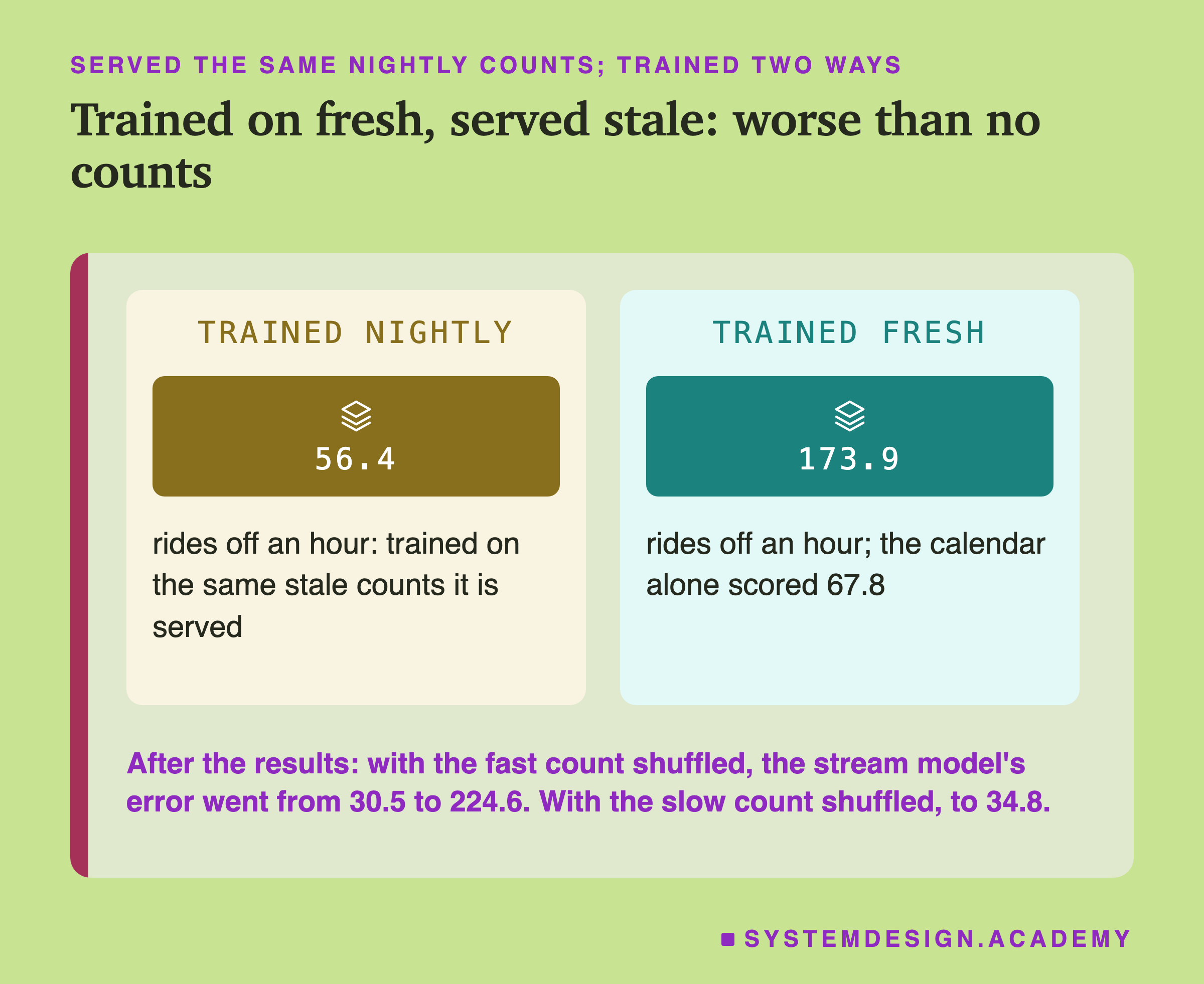
To see why, I shuffled one input at a time across the test hours, after the results, and measured the stream model again. Shuffling breaks the link between an input and the right answer.
Each value on its own is still a real count, but the pairs can be odd: a shuffled count can put 800 rides next to 03:00. So how much worse the model gets tells you roughly how much it leans on that input. With the fast count shuffled, its error went from 30.5 to 224.6. With the slow count shuffled, it went to 34.8. The stream model leaned heavily on the last hour's rides. Served 138 at 18:00 on 8 August, it guessed 183 for an hour that had 862 rides.
The nightly model learned from the same stale value it would later be served. Here is one possible reading, which I did not test on its own. A late-evening count told it little about 18:00. So it learned to lean on the calendar and the week's average instead, and a stale count could not mislead it much.
This is the rule that matters most in this lesson, and it is not batch or stream: train on the same numbers you will serve. A stale input with a model that learned from stale values was a moderate loss here. A stale input fed to a model that expects a fresh one was a large loss, and nothing raised an error.
The damage depends on which way the mismatch runs. After the results, I measured the reverse too: a model trained on the nightly counts and served fresh ones. It scored 61.3. That is far better than 173.9, but still worse than the 56.4 the same model scored when it was served the nightly counts it learned from. A fresher input did not help a model that had learned what stale ones mean. The chapter on why production breaks measured the same kind of failure for inputs computed a different way, such as temperatures sent in Fahrenheit. Here the value was right in every way except the moment it was computed.
How Often Must the Job Run?
Between a nightly job and a stream there is a whole range of choices: run the same batch job every few hours. Spark's Structured Streaming works close to this by default. Its documentation says queries "are processed using a micro-batch processing engine": small batch jobs run one after another. The demo measured the range, with both counts from a job run every 1, 2, 3, 6, 12 and 24 hours, each model trained and served alike.
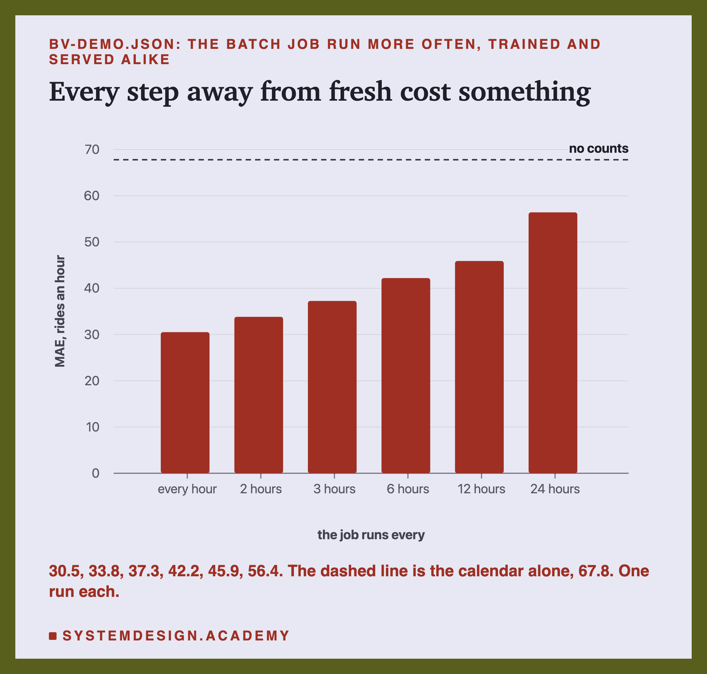
Every step away from fresh cost something. A job every hour scored 30.5, every 2 hours 33.8, and every 3 hours 37.3. Every 6 hours it scored 42.2, every 12 hours 45.9, and every 24 hours 56.4.
None of them came near the calendar alone, 67.8, so even a count from last night carried some information. How far the fast count was off rose from 38.0 rides for a job every 2 hours to 147.9 for a job every 6 hours. The job every 12 hours runs at 00:00 and at 12:00. Its fast count was off by a little less than the 6-hour one, 134.2, although its model still scored worse. I did not study why.
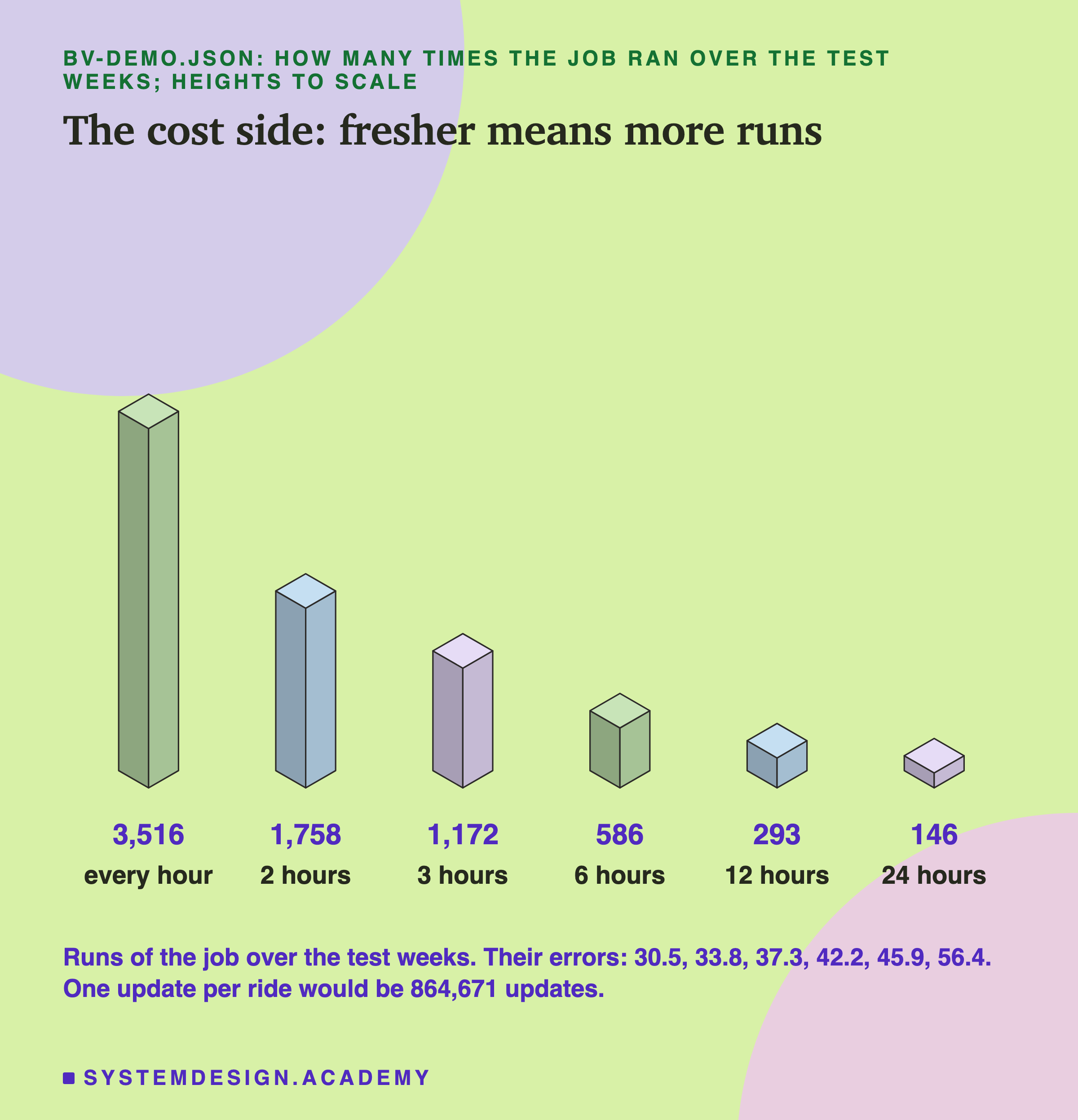
The other side of the trade is how often the job runs. Over the test weeks, a job every hour ran 3,516 times and a job every 24 hours ran 146 times. A real stream that updates on every ride would have done it 864,671 times. That count of runs is the real part of the cost here. What each run costs in money depends on the system, and I did not measure it.
So the practical question is not "batch or stream". It is: for this input, how much error does each extra run buy? Here, going from a job every 24 hours to a job every 3 hours cut the error from 56.4 to 37.3, for 1,172 runs instead of 146. Going the rest of the way to every hour cut it to 30.5, for 3,516. Whether that is worth it is a business question, and now it is one you can answer with numbers.
The Lambda Architecture: Have Both
For years, teams wanted the freshness of a stream and the exactness of batch at the same time. The Lambda architecture was the classic answer. Nathan Marz described it in a post called "How to beat the " (13 October 2011), with a batch layer and a realtime layer. The CAP theorem is a well-known result about systems spread over many machines. Sometimes part of the network is cut off from the rest, which is called a network partition. The theorem says that then the system has to give up either consistency or availability.
His book Big Data, written with James Warren, "presents the Lambda Architecture" under that name, and calls the fast path the speed layer.
The idea: send every event down two paths at once.
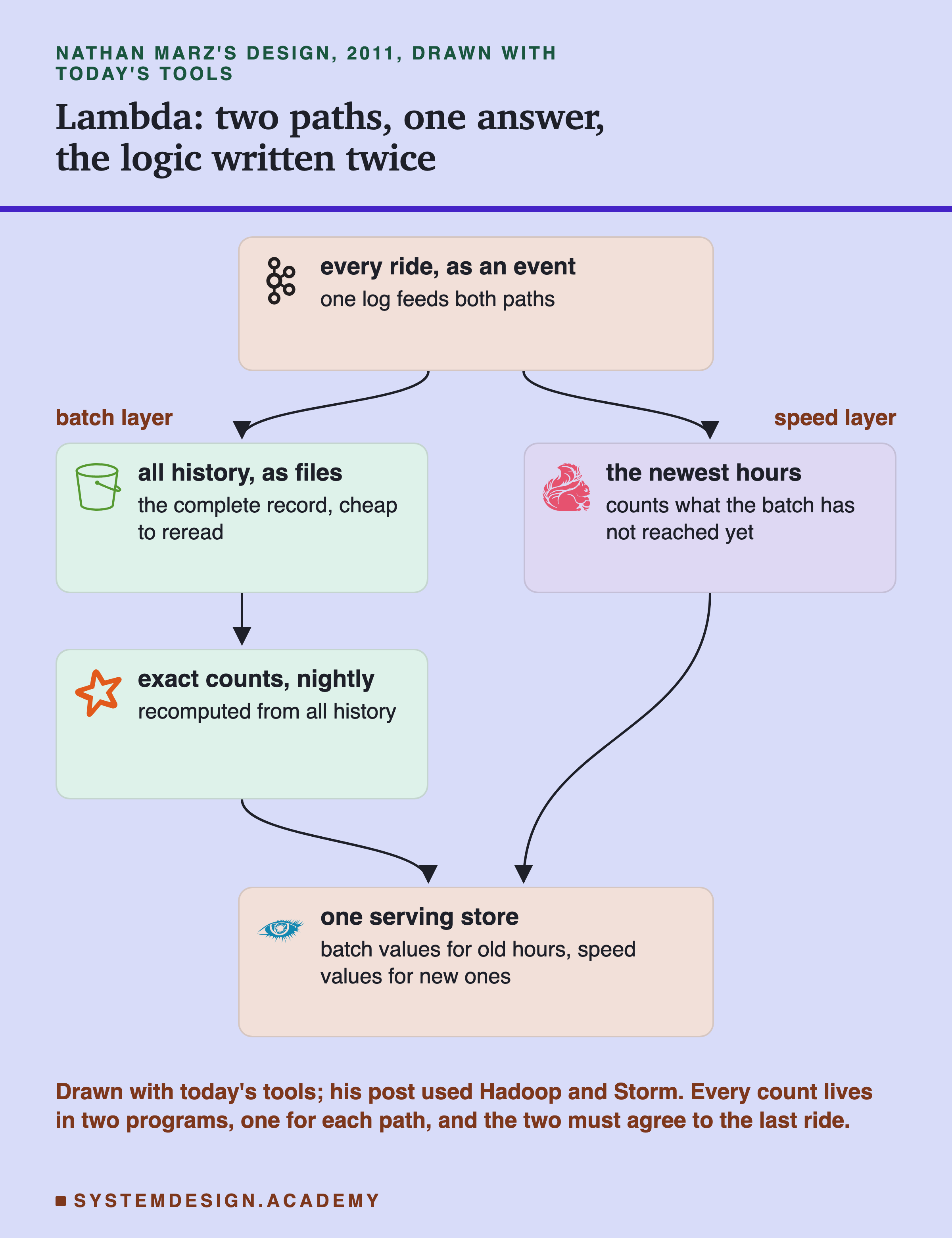
The batch layer rereads the full history and recomputes exact values. It is slow, running on a schedule, but its output is complete, so it is the source of truth. The speed layer follows the same events and covers the hours the batch layer has not reached yet.
A serving store merges the two. For older hours it serves the batch value. For the newest hours it serves the speed layer's value, until the batch layer catches up and replaces it. In Marz's own words: "everything the realtime layer computes is eventually overridden by the batch layer." Because its values only live until the exact batch value arrives, the speed layer can afford to be roughly right.
It works. But look at the diagram and you will see the tax: the same count is written twice, once for the batch engine and once for the stream engine. That is two programs that must agree exactly, or the model's inputs quietly change depending on which path produced them. Jay Kreps put it plainly in 2014. Keeping code that must give the same result in two systems, he wrote, "is exactly as painful as it seems like it would be."
The Kappa Architecture: Just Stream Everything
On 2 July 2014, Jay Kreps, one of the original creators of Apache , wrote "Questioning the Lambda Architecture" for O'Reilly Radar. His complaint was the tax on the last slide: why keep two copies of every computation? His answer was one path, the stream. He named it almost in passing: "Maybe we could call this the Kappa Architecture, though it may be too simple of an idea to merit a Greek letter."
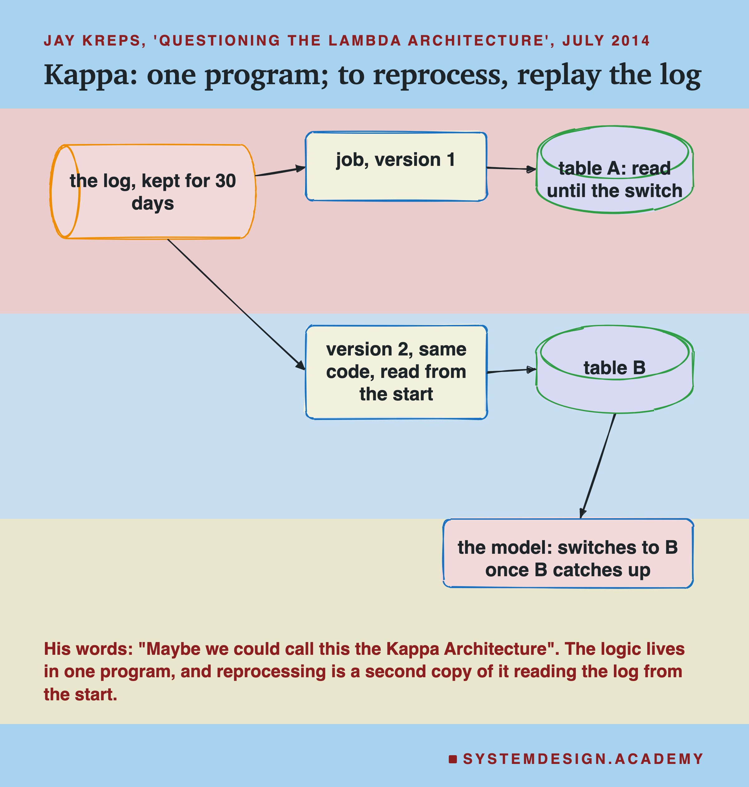
The trick is that the event log keeps enough history to serve as the source of truth. Reprocessing, the thing the batch layer was for, becomes a replay of the log. His recipe goes like this. First, keep as much history in Kafka as you may need to reprocess. In his words: "if you want to reprocess up to 30 days of data, set your retention in Kafka to 30 days."
When the logic changes, start a second copy of the same stream job. It reads from the beginning of the log and writes to a new table. When it has caught up, switch the application to the new table, then stop the old job and delete the old table. One program. Fix a bug once, and the replay applies the fix everywhere. The switch also gives you a clean way back: if the new version is wrong, you never switch, and the old job is still running.
The cost is real. A full recompute means replaying the whole log through a stream engine. A stream engine reads records one at a time and keeps a running state for each key, while a batch engine scans compressed files in bulk. For a pure historical total, batch is often the faster tool. And you must keep a lot of history in the log. Kafka can now move old parts of its log to cheap object storage. This tiered storage arrived as an early-access feature in Kafka 3.6 (October 2023). It was declared production-ready in Kafka 3.9 (November 2024).
Event Time, Processing Time, and Watermarks
The next idea decides whether a streaming input is right at all.
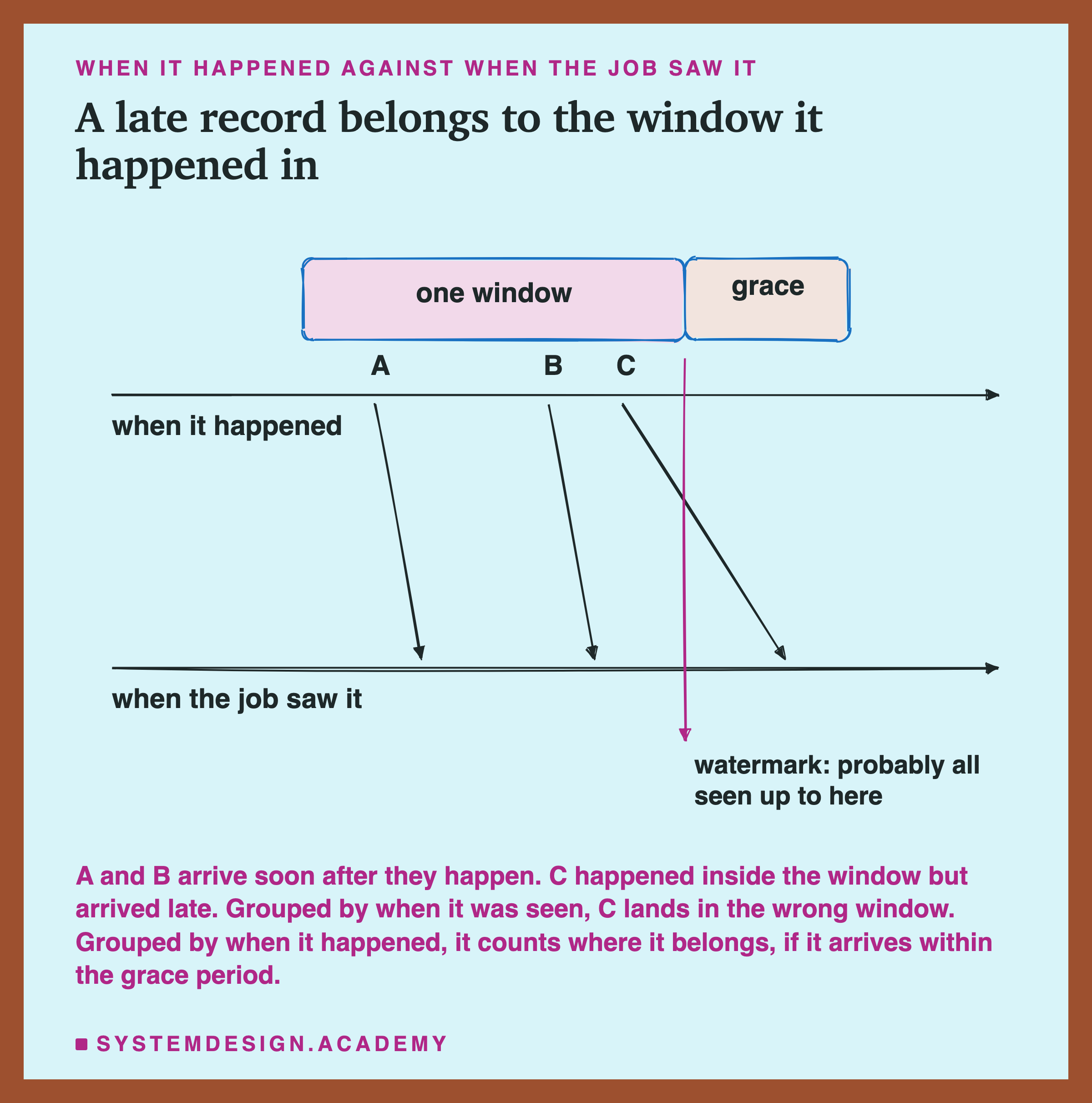
Event time is when a thing actually happened. Processing time is when your job saw it. In Akidau's words, event time is "the time at which events actually occurred" and processing time is the time "at which events are observed in the system". In a stream the two drift apart all the time, because networks lag and phones go through tunnels. A ride that really started at one moment might reach the job several seconds later.
It is tempting to say batch has no such problem, because all the data is already in the file. It has the same problem, hidden at the cut-off. A nightly job over "yesterday" reads whatever had arrived by 00:00. A record from 23:59 that arrives at 00:03 is simply missing from the result, and stays missing until someone runs the job again.
Akidau makes the same point about batch jobs that cut data into fixed windows. He asks: "what if some of your events are delayed en route to the logs due to a network partition?" A network partition is the break in the network described on the Lambda slide. The difference is that a stream has to decide, every minute, how long to wait.
Before the timing problem, there is a shape problem. You cannot count or average over an unbounded stream until you cut it into finite pieces, called windows. And the rule you pick for the cut changes the number. Apache Flink's documentation describes the three common choices.
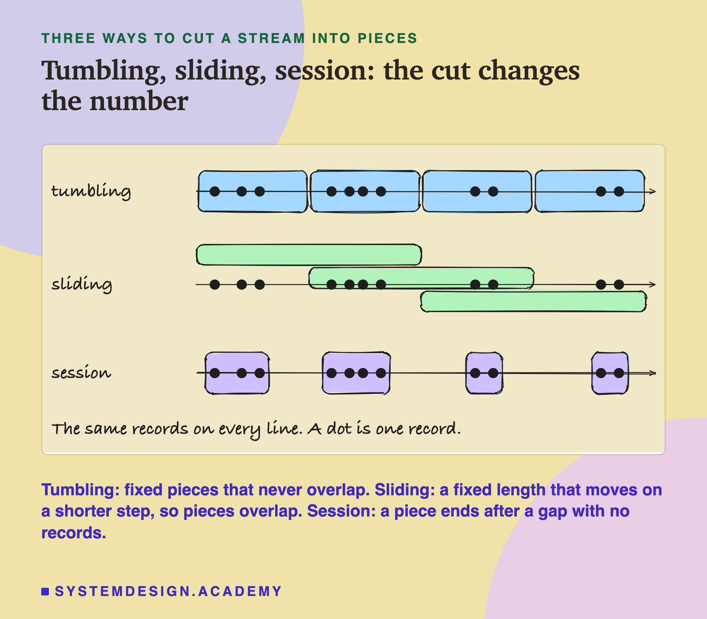
The window type is a modelling choice, not a detail. Tumbling windows "have a fixed size and do not overlap". They suit a number like rides per clock hour, the way the lab's data is cut. Sliding windows have a fixed size and move forward on a shorter step, so they overlap. They are how "transactions in the last 5 minutes" stays current every 30 seconds.
Exactly-Once vs At-Least-Once, and How This Feeds ML
One more streaming decision has direct consequences for your data: the delivery guarantee. Stream jobs crash and restart, and what the restart does to your counts is the delivery guarantee.
At-least-once means every record is processed, but after a crash some may be processed twice. Flink's documentation says it plainly: "Nothing is lost, but you may experience duplicated results (at least once)". For a count, a duplicate is an extra.
Exactly-once means every record affects the result one time, even across crashes. The name describes the effect on the result, not on the wire. A record may still be read again after a crash, but it lands in the result once. Flink does this by saving its state together with its position in the input, which is called a checkpoint.
The promise holds end to end only if the place the job writes to takes part. In Flink's words, "your sources must be replayable, and your sinks must be transactional (or idempotent)". A sink is where the job writes its results. Idempotent means that writing the same thing twice leaves the same result as writing it once. A producer is the program that writes records into , and a transaction is a group of writes that either all become visible or none do. Kafka added idempotent producers and transactions in version 0.11, in 2017, so that the log itself can take part.
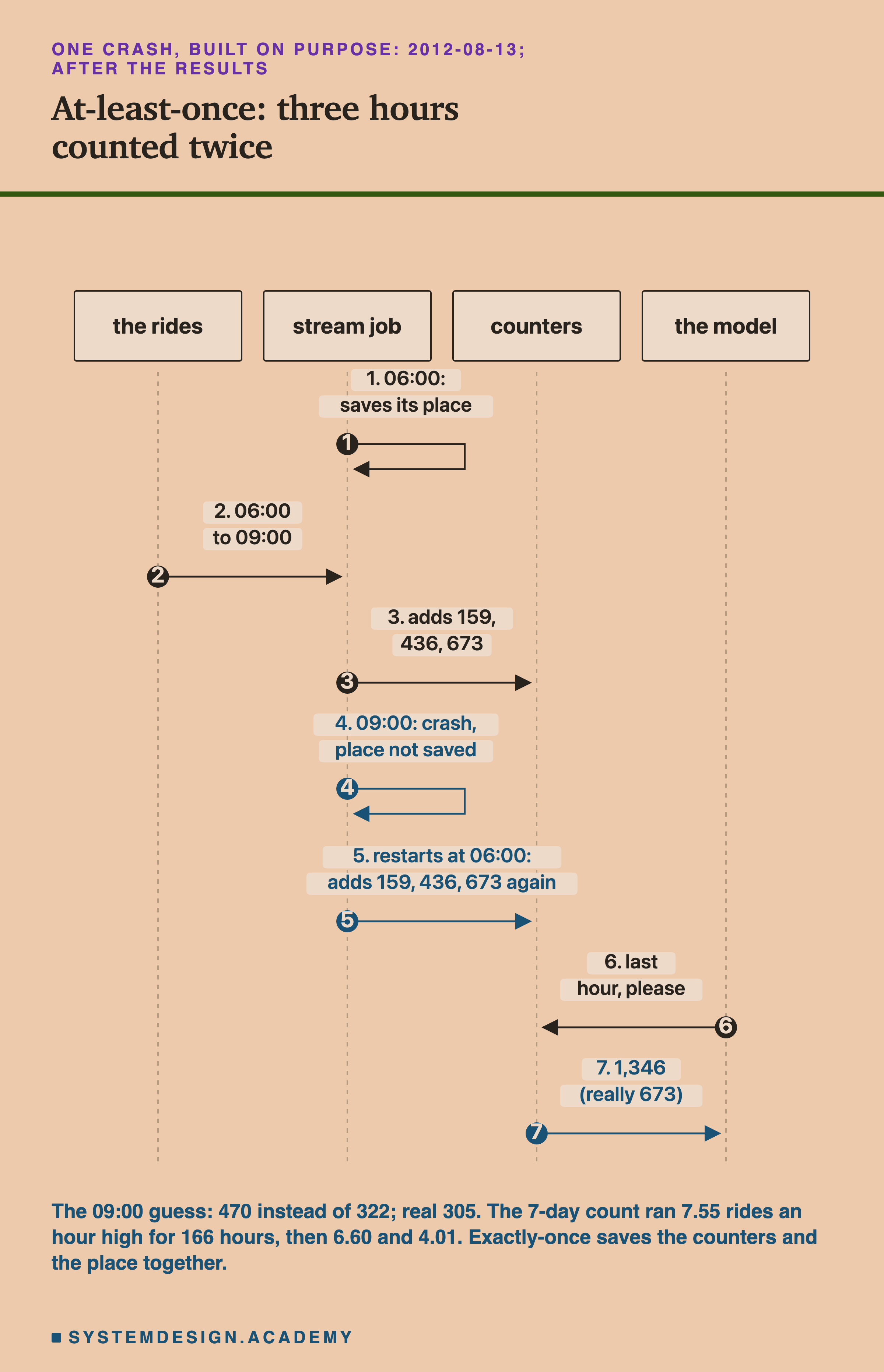
After the results, I built one crash on purpose, on the real data, to see what a duplicate does to a count. The stream job keeps one counter per clock hour in a database, and adds one to it for every ride. The fast count reads the last hour's counter, and the slow count sums the last 168.
The job records how far it got every 6 hours. It crashes once, at the start of 09:00 on Monday 13 August 2012, the first Monday of the test. It has counted 06:00, 07:00 and 08:00, but has not yet recorded that it did. On restart it goes back to 06:00 and counts those three hours again.
How Uber, Netflix, and DoorDash Actually Split It
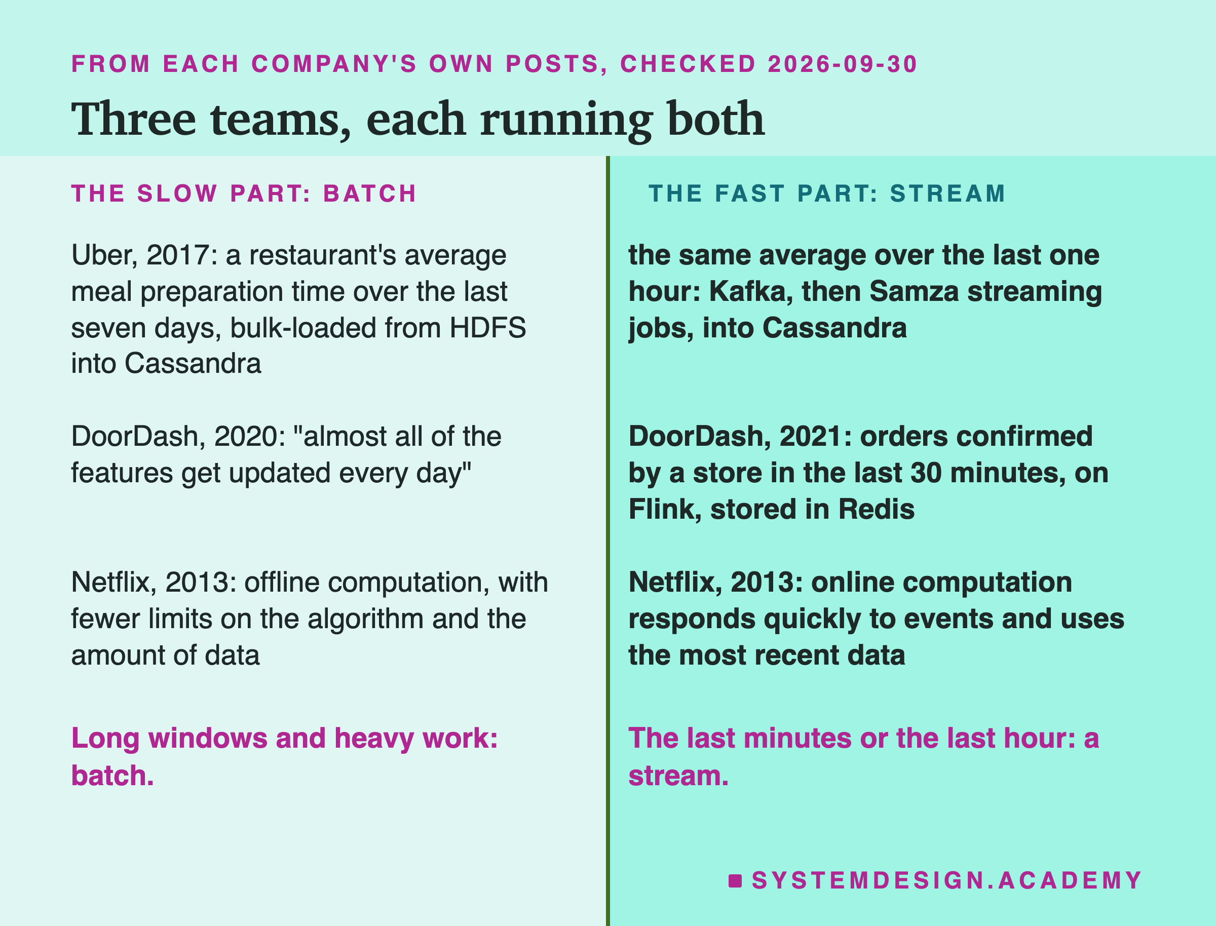
Three teams that wrote about their systems each run both batch jobs and streams. I checked every quote below against the company's own post on 30 September 2026.
Uber's 2017 post about its Michelangelo platform, by Jeremy Hermann and Mike Del Balso, describes two ways its models' inputs are computed. Three names in it need a word each. HDFS, the Hadoop Distributed File System, stores very large files across many machines. Apache Cassandra is a database that spreads its data over many machines. Samza is a stream processing framework, like Flink. The first is "bulk precomputing and loading historical features from HDFS into Cassandra on a regular basis": batch. The second is to "publish relevant metrics to Kafka and then run Samza-based streaming compute jobs to generate aggregate features at low ": a stream.
Its example is the same pair as this lesson's lab. UberEATS computes "a restaurant's average meal preparation time over the last seven days" in batch, and the same average "over the last one hour" in the stream. The streaming values are also logged back to HDFS for later training. The post says the near-real-time path "ensures that the same data is used for training and serving": this lesson's skew rule, built into the platform.
DoorDash wrote in 2020, in a post by Arbaz Khan and Zohaib Sibte Hassan, that "almost all of the features get updated every day". Its example of a real-time input, "average delivery time for orders from a store in the past 20 minutes", is instead "updated uniformly throughout the day". In 2021, Allen Wang and Kunal Shah described Riviera, a framework built on Apache Flink that computes such inputs. One example is the "total orders confirmed by a store in the last 30 minutes", over a rolling window that refreshes every minute.
Riviera serves them from a built on Redis: a system that keeps a model's input values ready to be read quickly.
Netflix wrote in 2013, in a post by Xavier Amatriain and Justin Basilico, that its recommendations are computed in three ways. Offline computation "allows for more choices in algorithmic approach such as complex algorithms and less limitations on the amount of data that is used". Online computation "can respond quickly to events and use the most recent data". Nearline computation sits between the two, and stores its results instead of serving them at once. Netflix's Keystone platform runs its streams on and Flink (2018), and a 2022 paper describes Netflix search adapting to members' "interactions from the current session".
Try It Yourself
This script is the lab. It downloads the Bike Sharing data and rebuilds the clock. It computes the two counts as a stream and as a nightly job would, and trains the five designs. Then it runs the batch job every 1, 2, 3, 6, 12 and 24 hours. It prints each design's error, how far the nightly counts are from fresh ones, and how many times each job ran. It does not need a GPU; when I ran it, it finished in under ten seconds.
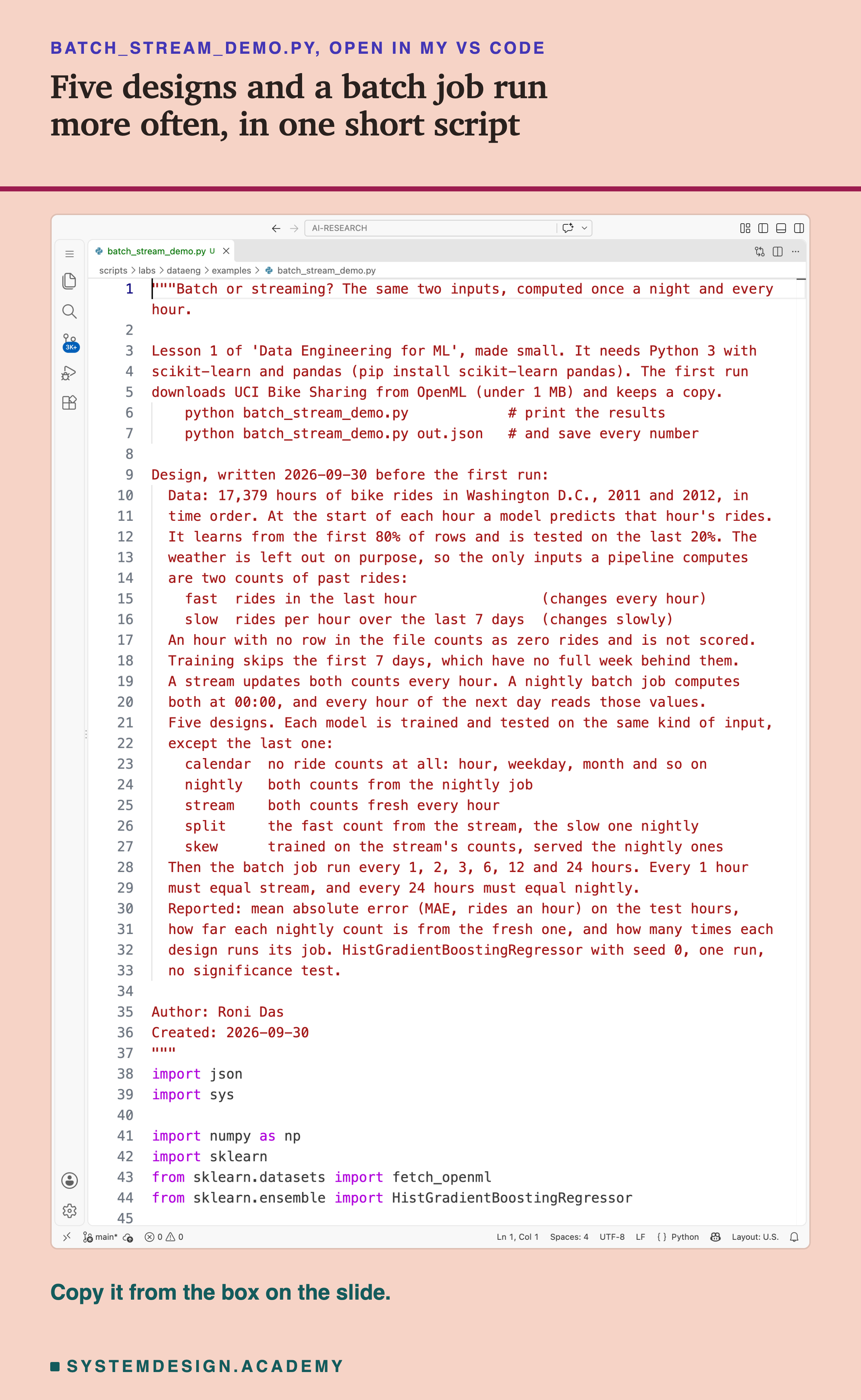
Before you run this lab. You need Python 3 and two libraries: pip install scikit-learn pandas. scikit-learn holds the model and the download, and brings NumPy with it; pandas holds the table. The first run downloads the Bike Sharing data from OpenML (under 1 MB), so it needs an internet connection once. After that, scikit-learn keeps a copy in a folder in your home directory (scikit_learn_data).
I ran it with scikit-learn 1.9.1 on a Mac. scikit-learn runs the same way on Windows and Linux, but I have not checked the numbers there. Another version of scikit-learn may give different decimals, which is why the first line printed is the version. Give it a file name, python batch_stream_demo.py out.json, and it also saves every number at full precision; that is how results/bv-demo.json was made.
"""Batch or streaming? The same two inputs, computed once a night and every hour.

Lesson 1 of 'Data Engineering for ML', made small. It needs Python 3 with
scikit-learn and pandas (pip install scikit-learn pandas). The first run
downloads UCI Bike Sharing from OpenML (under 1 MB) and keeps a copy.
    python batch_stream_demo.py            # print the results
    python batch_stream_demo.py out.json   # and save every number

Design, written 2026-09-30 before the first run:
  Data: 17,379 hours of bike rides in Washington D.C., 2011 and 2012, in
  time order. At the start of each hour a model predicts that hour's rides.
  It learns from the first 80% of rows and is tested on the last 20%. The
  weather is left out on purpose, so the only inputs a pipeline computes
  are two counts of past rides:
    fast  rides in the last hour               (changes every hour)
    slow  rides per hour over the last 7 days  (changes slowly)
  An hour with no row in the file counts as zero rides and is not scored.
  Training skips the first 7 days, which have no full week behind them.
  A stream updates both counts every hour. A nightly batch job computes
  both at 00:00, and every hour of the next day reads those values.
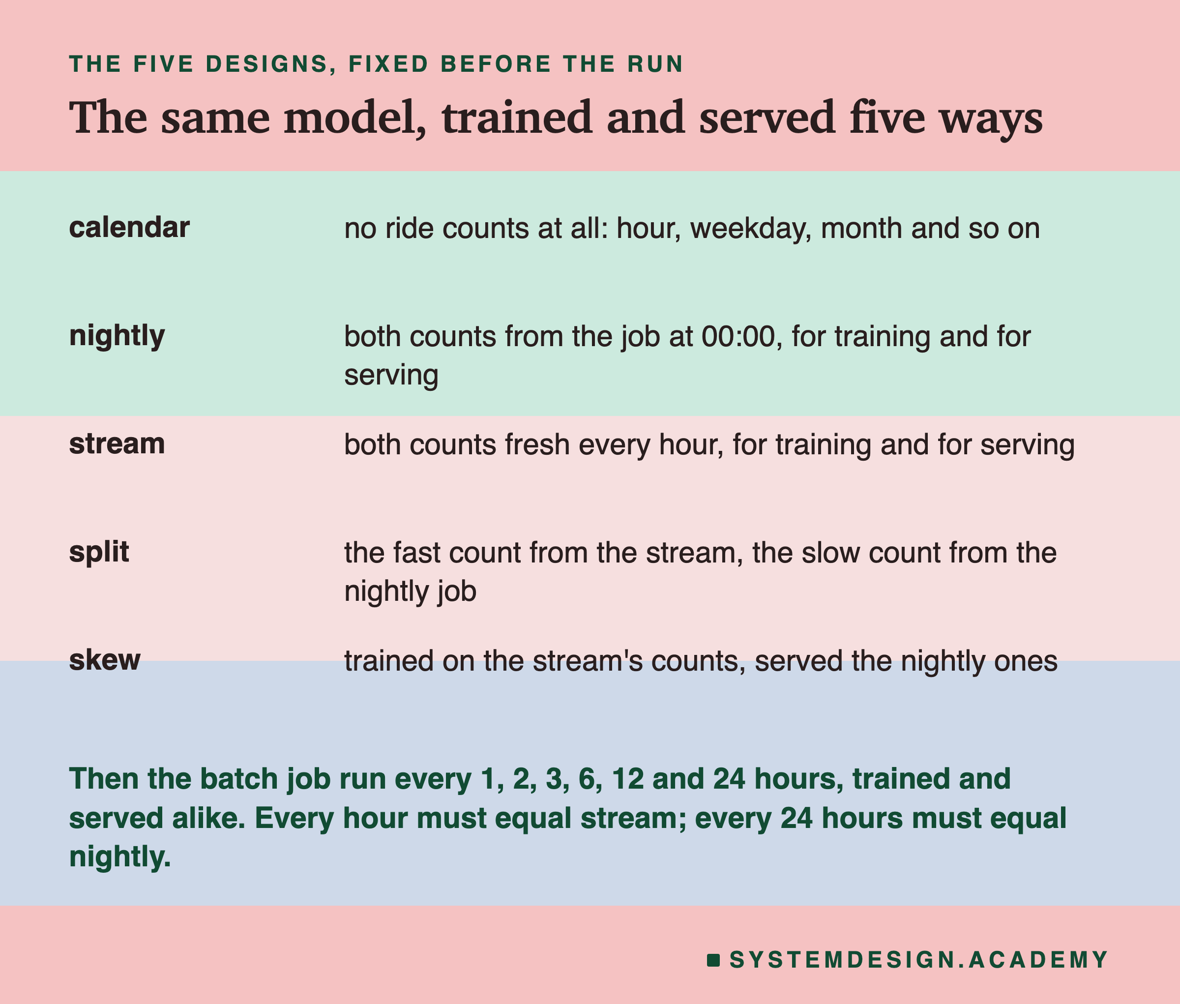
  Five designs. Each model is trained and tested on the same kind of input,
  except the last one:
    calendar  no ride counts at all: hour, weekday, month and so on
    nightly   both counts from the nightly job
    stream    both counts fresh every hour
    split     the fast count from the stream, the slow one nightly
    skew      trained on the stream's counts, served the nightly ones
  Then the batch job run every 1, 2, 3, 6, 12 and 24 hours. Every 1 hour
  must equal stream, and every 24 hours must equal nightly.
  Reported: mean absolute error (MAE, rides an hour) on the test hours,
  how far each nightly count is from the fresh one, and how many times each
  design runs its job. HistGradientBoostingRegressor with seed 0, one run,
  no significance test.

Author: Roni Das
Created: 2026-09-30
"""
import json
import sys

import numpy as np
import sklearn
from sklearn.datasets import fetch_openml
from sklearn.ensemble import HistGradientBoostingRegressor

data = fetch_openml("Bike_Sharing_Demand", version=2, as_frame=True, parser="auto").frame
rides = data["count"].to_numpy()

# The file has the year, month, weekday and hour, but no day of the month.
# A new day starts when the weekday changes; a jump of two skips a day.
weekday, hour = data["weekday"].to_numpy(), data["hour"].to_numpy()
day = np.r_[0, np.cumsum((weekday[1:] - weekday[:-1]) % 7)]
clock = day * 24 + hour  # hours since 2011-01-01 00:00

# Rides on a full hourly clock. total[k] is every ride before hour k.
on_clock = np.zeros(clock[-1] + 1, dtype=int)
on_clock[clock] = rides
total = np.r_[0, np.cumsum(on_clock)]


def counts(asof):
    """The two inputs as a job that ran at the start of hour `asof` saw them.

    The first week's rows get meaningless values here; none is used."""
    fast = total[asof] - total[asof - 1]
    slow = (total[asof] - total[asof - 168]) / 168
    return fast, slow


calendar = np.column_stack([
    hour, weekday, data["month"], data["year"],
    data["workingday"].astype(str) == "True", data["holiday"].astype(str) == "True",
]).astype(float)


def table(fast_every=None, slow_every=None):
    """The calendar, plus each count from a job run every N hours."""
    cols = [calendar]
    if fast_every:
        cols.append(counts(clock // fast_every * fast_every)[0])
    if slow_every:
        cols.append(counts(clock // slow_every * slow_every)[1])
    return np.column_stack(cols)


cut = int(0.8 * len(rides))  # learn from the first 80% of rows
train = np.flatnonzero((np.arange(len(rides)) < cut) & (clock >= 168))
test = np.arange(cut, len(rides))


def mae(learn_from, serve_with):
    model = HistGradientBoostingRegressor(random_state=0)
    model.fit(learn_from[train], rides[train])
    error = model.predict(serve_with[test]) - rides[test]
    return float(np.abs(error).mean())


out = {"scikit_learn": sklearn.__version__, "rows": len(rides),
       "train_rows": len(train), "test_rows": len(test),
       "hours_without_a_row": int(len(on_clock) - len(rides)),
       "test_mean_rides": float(rides[test].mean())}
print(f"scikit-learn {sklearn.__version__}, {len(test):,} test hours")
print(f"real rides an hour in the test: {rides[test].mean():.1f}")

X = {"calendar": table(), "nightly": table(24, 24),
     "stream": table(1, 1), "split": table(1, 24)}
out["mae"] = {name: mae(X[name], X[name]) for name in X}
out["mae"]["skew"] = mae(X["stream"], X["nightly"])
print("error (MAE, rides an hour), one run each:")
for name, value in out["mae"].items():
    print(f"  {name:<9} {value:6.1f}")

# How far the nightly job's counts are from fresh ones, on the test hours.
fresh, night = counts(clock), counts(clock // 24 * 24)
out["nightly_off_by"] = {k: float(np.abs(night[i] - fresh[i])[test].mean())
                         for i, k in enumerate(["fast", "slow"])}
print("nightly count off from the fresh one, on average:")
print(f"  fast  {out['nightly_off_by']['fast']:6.1f} rides")
print(f"  slow  {out['nightly_off_by']['slow']:6.1f} rides an hour")

# The same batch job, run more often: both counts, trained and served alike.
out["every"] = {}
print("batch job every N hours: runs in the test, MAE")
for n in [1, 2, 3, 6, 12, 24]:
    runs = int(clock[-1] // n - (clock[cut] - 1) // n)  # starts in the test
    out["every"][n] = {"runs": runs, "mae": mae(table(n, n), table(n, n))}
    print(f"  every {n:>2}h {runs:>6,} runs  {out['every'][n]['mae']:6.1f}")
out["test_rides"] = int(rides[test].sum())
print(f"one update per ride instead: {out['test_rides']:,}")

if len(sys.argv) > 1:  # a file name was given: save every number too
    json.dump(out, open(sys.argv[1], "w"), indent=1)
The Lab Report
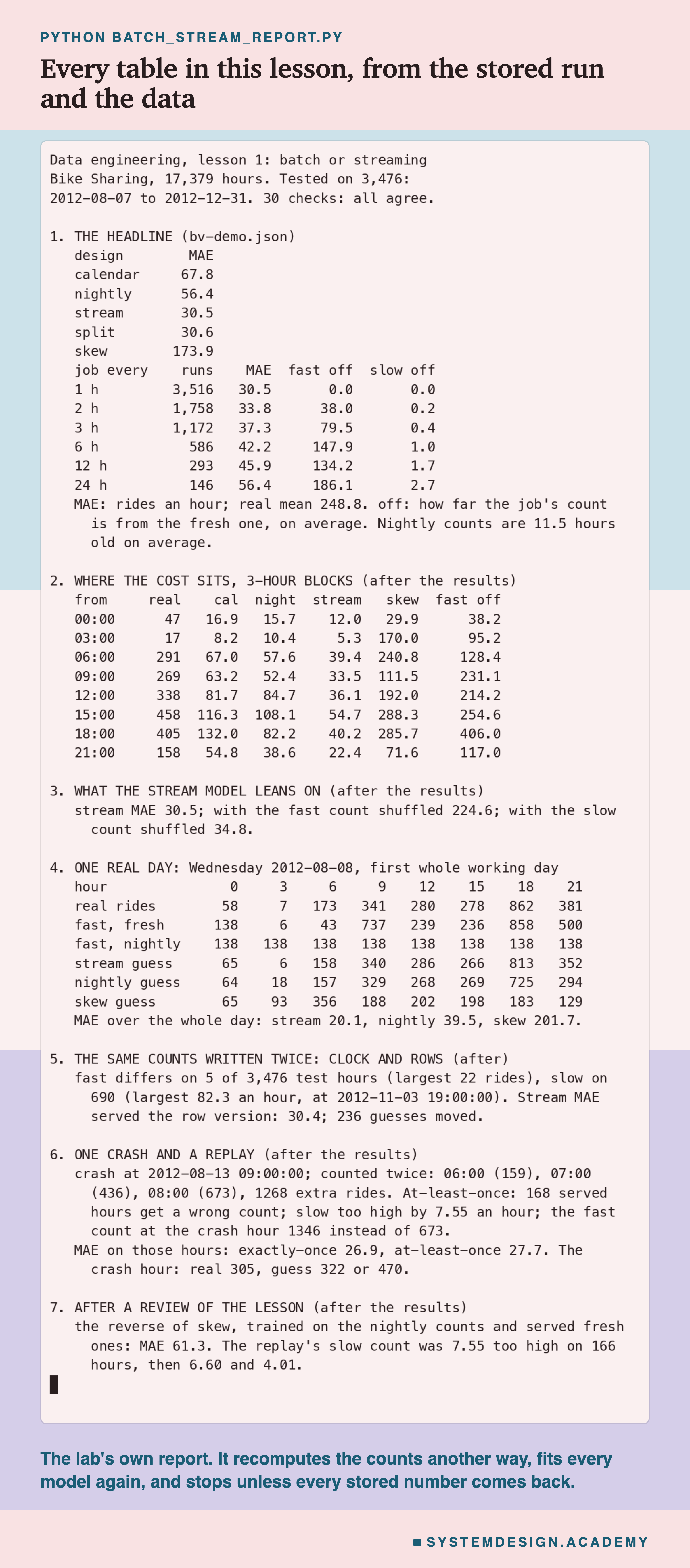
The report lives in scripts/labs/dataeng/batch_stream_report.py. It reads the demo's stored files, results/bv-demo.json and the printed run, and the Bike Sharing data from scikit-learn's local copy. It does not trust the demo's arithmetic. It rebuilds the calendar with real dates, and checks it against every row's year, month and weekday. It computes the two counts a different way, with pandas on an hourly clock instead of the demo's running total. It fits every model again. And it stops unless every stored error, count and run comes back exactly. Every check agreed. It changes nothing in the demo's files.
Its json mode writes every number to results/bv-report.json, which the figures read. The demo mode checks the demo's printed run line by line, and the box mode writes the playground below and checks it against both files.
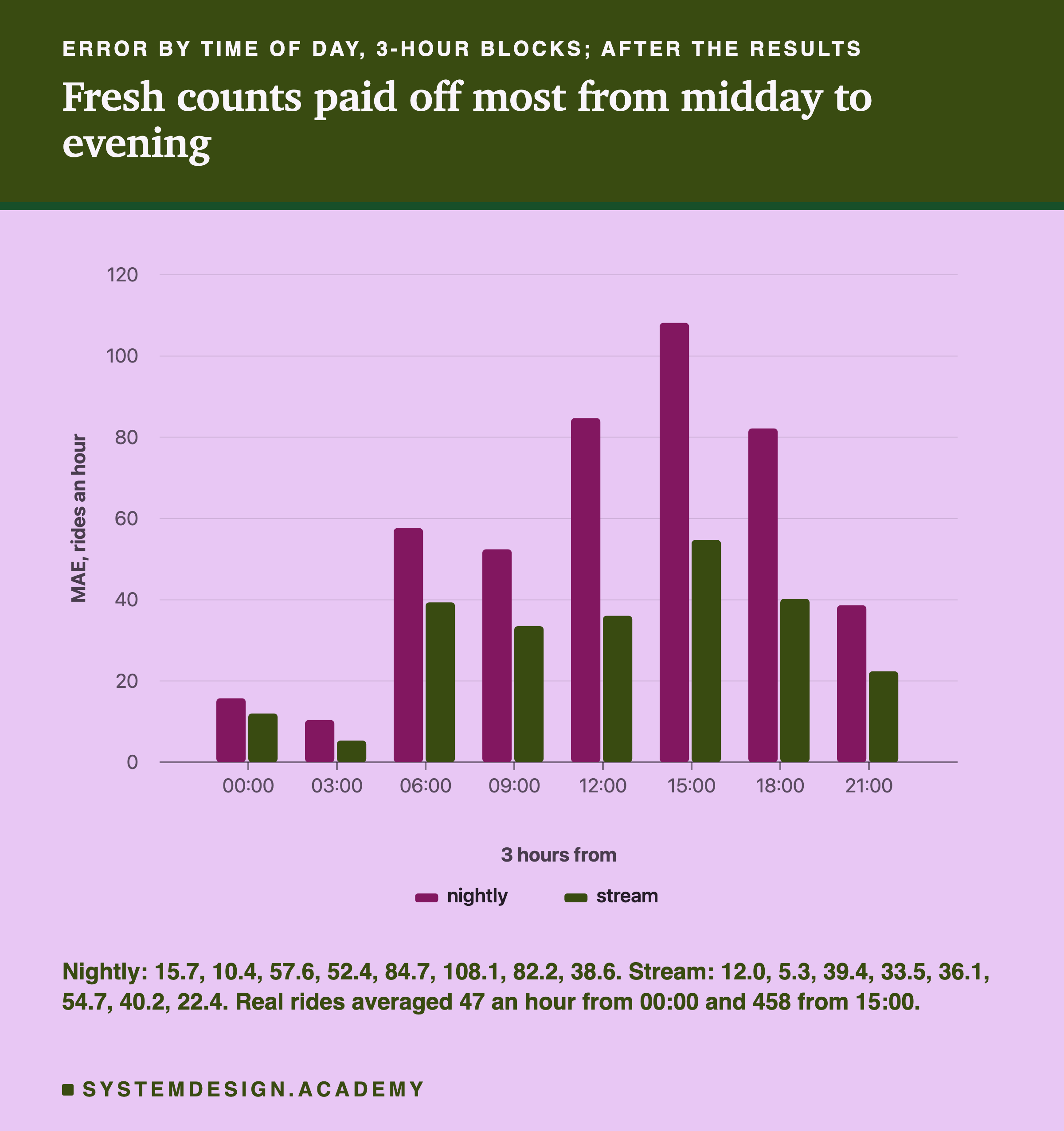
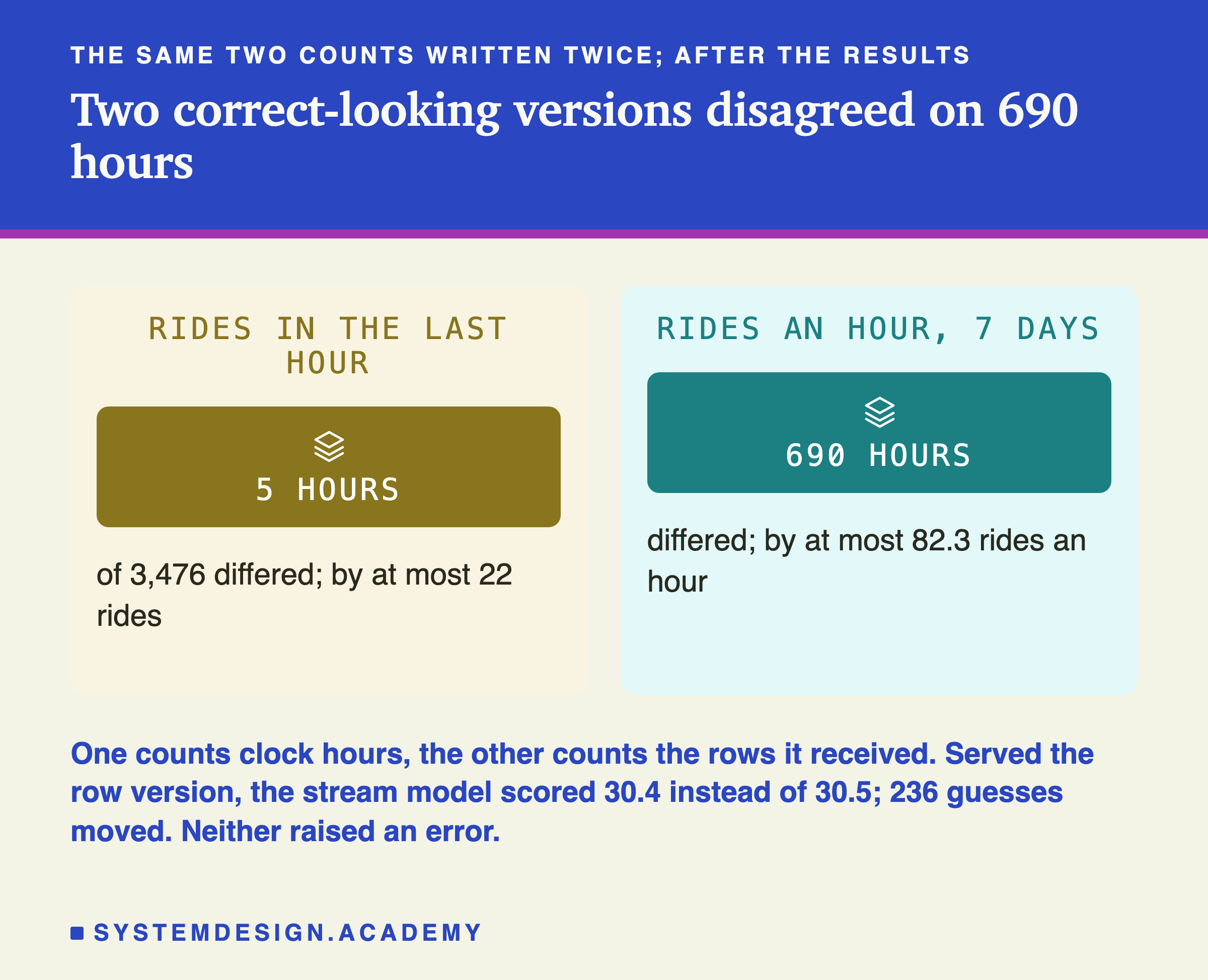
Here is what came before the run, in the demo's docstring: the data, the split, the two counts and the five designs. The job every 1 to 24 hours, and what to report, were there too. Then there is what came after I saw the results, written into the report's docstring before the report first ran. It covers the error by time of day, the shuffles, and the sketched day with the rule that picked it. It also covers the two versions of the counts, and the crash and replay. Every figure that shows one of those says "after the results".
Count It Yourself, No Model
This box has no model in it. It holds the real rides for every clock hour, from eight days before the test to the end of 2012. It also holds the guesses of three designs, stream, nightly and skew, for every test hour, to a hundredth of a ride. Each number is stored as two or three characters, in base 64, so that the box stays small. Base 64 just means counting with 64 different digits instead of 10. It runs in your browser.
The counts in the box are exact. So how far a job's counts are from fresh ones matches the lab to the last digit. The report checked that for a job every 1, 2, 3, 6, 12 and 24 hours. The guesses are stored to a hundredth of a ride. The report checked that every MAE the box prints, for the whole test and for each 3-hour block, reads the same as the lab's.
As it is, the box prints the number of test hours, their real mean, and the MAE of the three designs. Then it prints how far two jobs are off from fresh counts. A job run every 24 hours is off by 186.1 and 2.7, and a job run every hour by 0.0.
Then try off(3) and off(6) to see how far a job every 3 or 6 hours is off. Compare them with the chart of errors on the slide about how often the job must run. Try by_block('skew') next to by_block('nightly') to see where in the day the skewed model went wrong, and mae('stream', range(15, 18)) for one block on its own. Ask yourself which of these you could have measured before building anything.
The Code, Part by Part
Loading. fetch_openml("Bike_Sharing_Demand", version=2) downloads the data once and reads the local copy after that. rides is the number of rides in each row's hour.
The clock. The file has no day of the month, so day counts days. Each step between two rows adds the change in weekday, taken modulo 7 (the remainder after dividing by 7). That change is 0 within a day, 1 at midnight, and 2 when a whole day has no row. clock is then the number of hours since 00:00 on 1 January 2011. on_clock puts every row's rides at its clock hour, with zero for the 165 hours that have no row. total is a running total: total[k] is every ride before hour k.
counts(asof). The two inputs as a job that ran at the start of hour asof would have seen them. The fast count is total[asof] - total[asof - 1], the rides in the hour before. The slow count is the rides in the 168 hours before, divided by 168. Because both use the running total, each count is one subtraction.
table. The calendar columns, plus each count from a job run every N hours. clock // N * N is the start of the hour when that job last ran, so is the stream, the nightly job and the split.
How to Choose, One Input at a Time
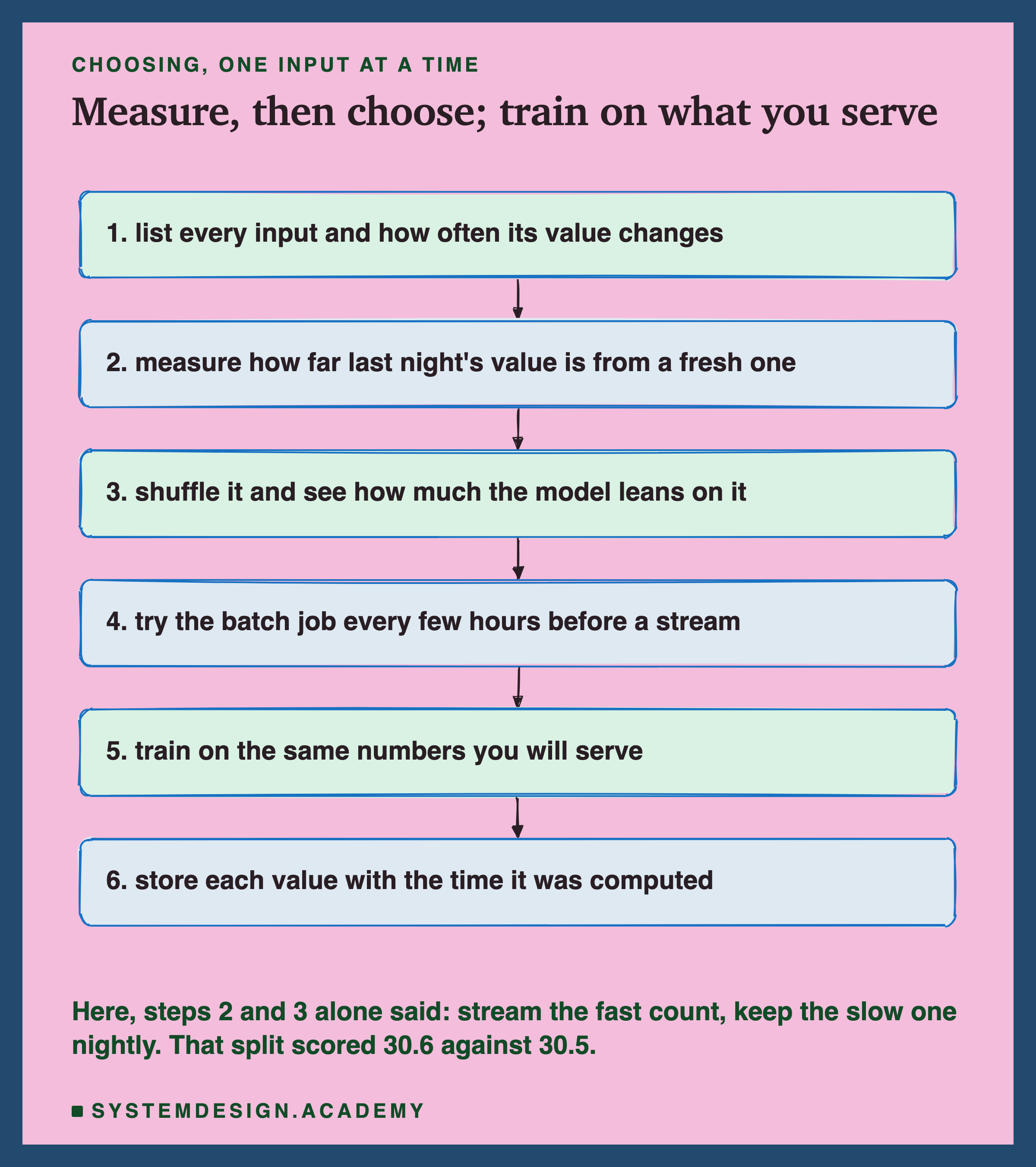
List every input and how often its value changes. A customer's country barely changes. A week's average changes a little every hour. A count over the last hour changes completely every hour. Write it down for each input before you choose anything.
Measure how far last night's value is from a fresh one. On past data, compute each input the way a nightly job would and the way a stream would, and average the difference. It needs no model. Here it was 186.1 rides for the fast count and 2.7 rides an hour for the slow one, and those two numbers alone pointed at the right design.
See how much the model leans on it. Shuffle the input across rows and measure the model again. If the error barely moves, freshness cannot matter much for that input.
Try a batch job every few hours before a stream. It is the same code as the nightly job, run more often. Here a job every 3 hours scored 37.3 against 56.4 for a nightly one.
Train on the same numbers you will serve. Build the training table the same way the serving path computes its inputs. Here, training on fresh counts and serving nightly ones cost more than any other choice: 173.9. The reverse, which I measured after the results, cost less, 61.3 against 56.4, but still more than training and serving alike.
Store each value with the time it was computed. Then how old an input is becomes a number you can check, and a stale input can raise an alarm instead of passing silently.
When to Stream, When to Batch
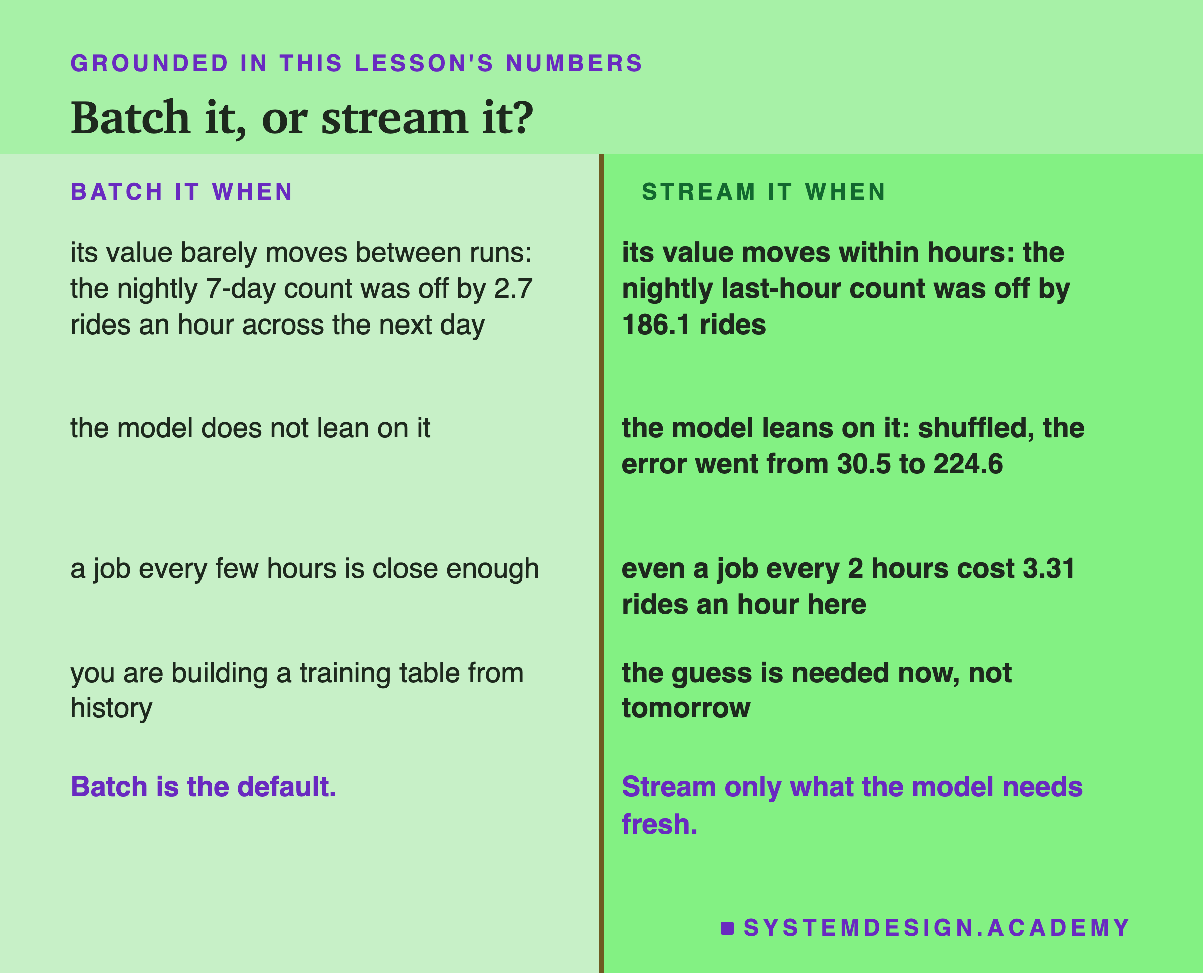
Batch it when its value barely moves between runs. A 7-day average, a customer's country, last month's total. Here the nightly 7-day count was off from the fresh value by 2.7 rides an hour on average, across the next day. Keeping it nightly cost 0.09 rides an hour.
Batch it when the model does not lean on it. Even a fast-moving input is not worth a stream if shuffling it barely changes the error.
Batch it when a job every few hours is close enough. It keeps the simplicity of batch: a job that starts and stops, and runs again on the same files after a failure.
Batch it for training data. Months of history, computed cheaply and exactly, is what a batch job is for, as long as serving computes the same thing.
Stream it when its value moves within hours and the model leans on it. Here the nightly last-hour count was off from the fresh value by 186.1 rides on average, across the next day. Shuffling it took the error from 30.5 to 224.6. That input earned its stream.
Stream it when the guess is needed now. A card payment, a delivery estimate, a bike dock about to run empty. If a guess from last night's numbers is no use by the morning, the input that drives it must be fresh.
Do not stream everything because it sounds modern. A stream runs all the time, needs a watermark, a delivery guarantee and someone on call. Pay for it only for the inputs that need it.
What These Numbers Can and Cannot Tell You
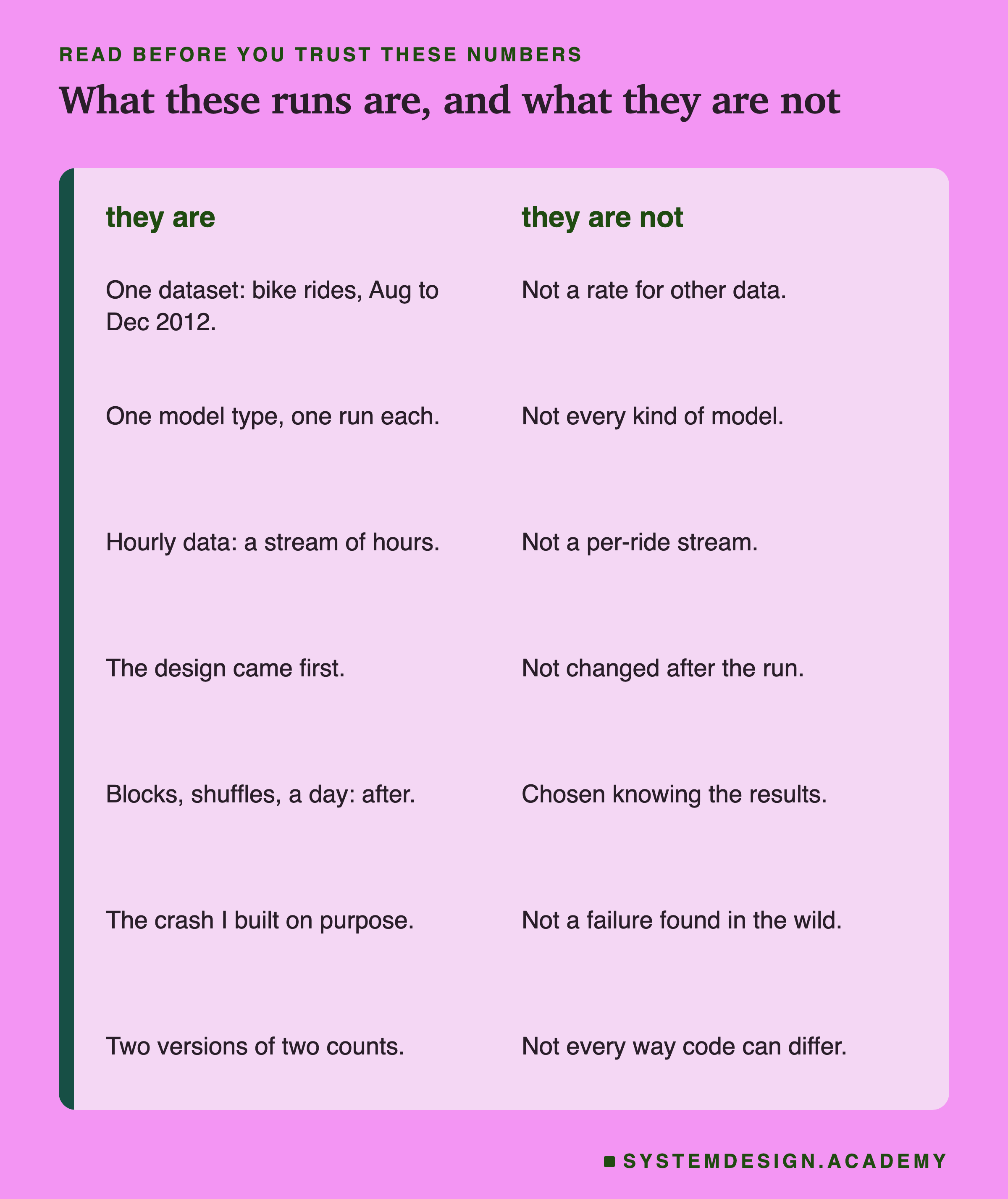
One dataset, one model type, one run each. Everything here is one city's bike rides in the second half of 2012, and one kind of model. With other data, other inputs and other models, the numbers would move. No significance test was declared, so I do not call any gap significant. The 0.09 between split and stream is too small to read anything into; what the split shows is that one count carried nearly all of the gain.
A stream of hours, not of rides. The data only has hourly totals, so my "stream" updates once an hour. A real stream updates on every ride, which would make the fresh count fresher still. I did not measure event time, watermarks or late records for the same reason.
No money. I counted how many times each job ran. What a run costs depends on the system, and I did not measure it.
The design came first. The five designs and the job every 1 to 24 hours were written down before the first run and not changed. The time-of-day blocks, the shuffles, the sketched day, the two versions of the counts and the crash came later. I designed them after I saw the results, and wrote them down before the report first ran. The reason I give for the nightly model's resistance to stale counts is my reading, labelled as such.
Faults I built on purpose. The crash, the replay and the second version of the counts are faults I put in to measure them. They are the kind of fault that happens in real systems, but they are not failures I found in someone's system.
What to Do Next
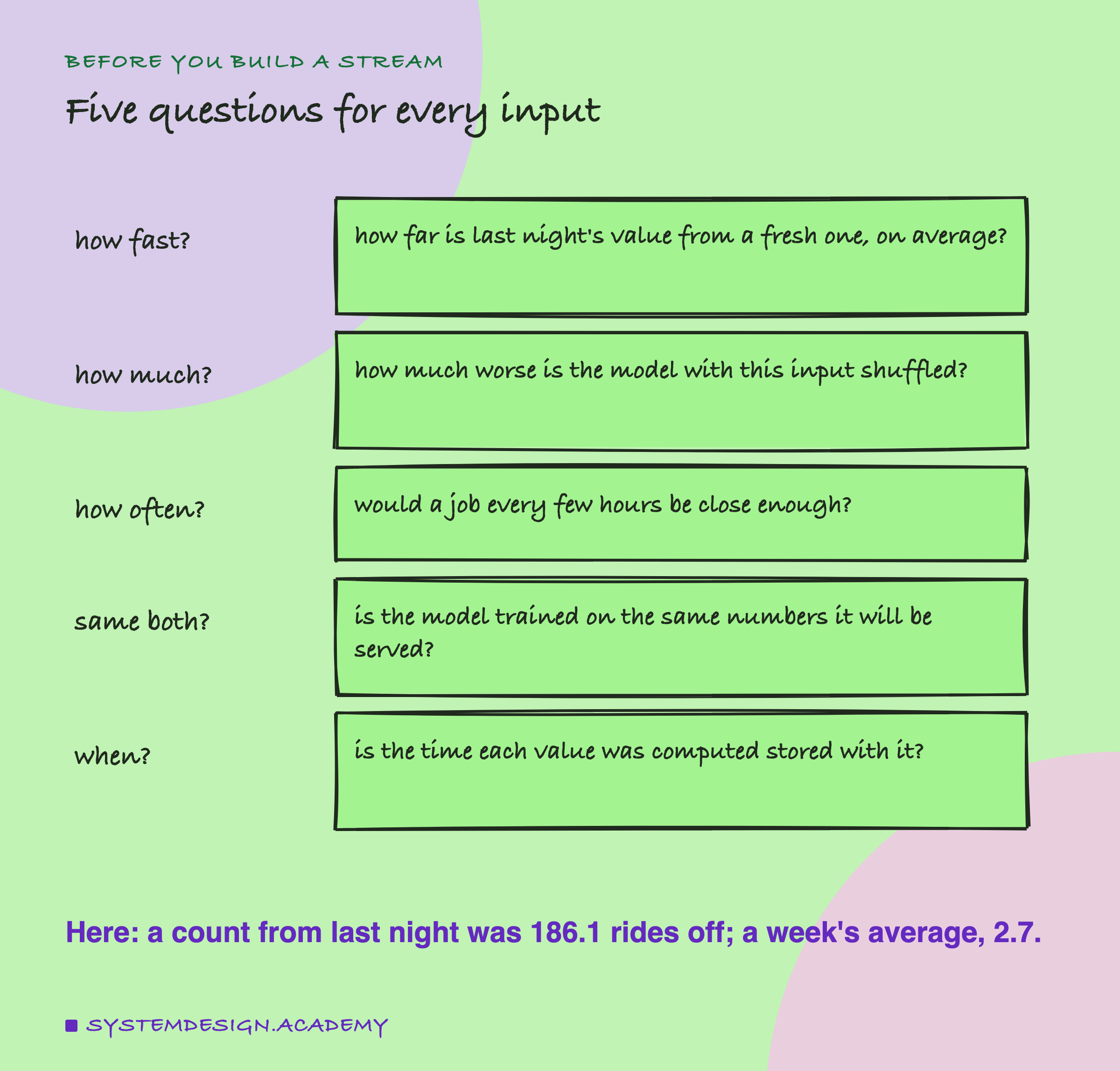
Take a model your team runs and list every input it reads. For each one, ask the five questions on the card. The first two need only past data and an afternoon. Compute each input the nightly way and the fresh way, and average the difference. Then shuffle it to see how much the model leans on it. Most inputs will turn out to be like the 7-day count, and they can stay in batch. A few will be like the last-hour count, and those are the ones worth a stream.
Then check the fourth question for every input: is the model trained on the same kind of number it is served? The skew design in this lesson is the common way to get it wrong. The training table is built from fresh values for every past hour, because history makes that easy. Serving, meanwhile, reads a table the nightly job refreshes once a day.
Here that cost more than anything else measured: 173.9. The reverse costs less but is still a mistake. After the results I trained on the nightly counts and served fresh ones. It scored 61.3, worse than the 56.4 of serving the nightly counts it learned from.
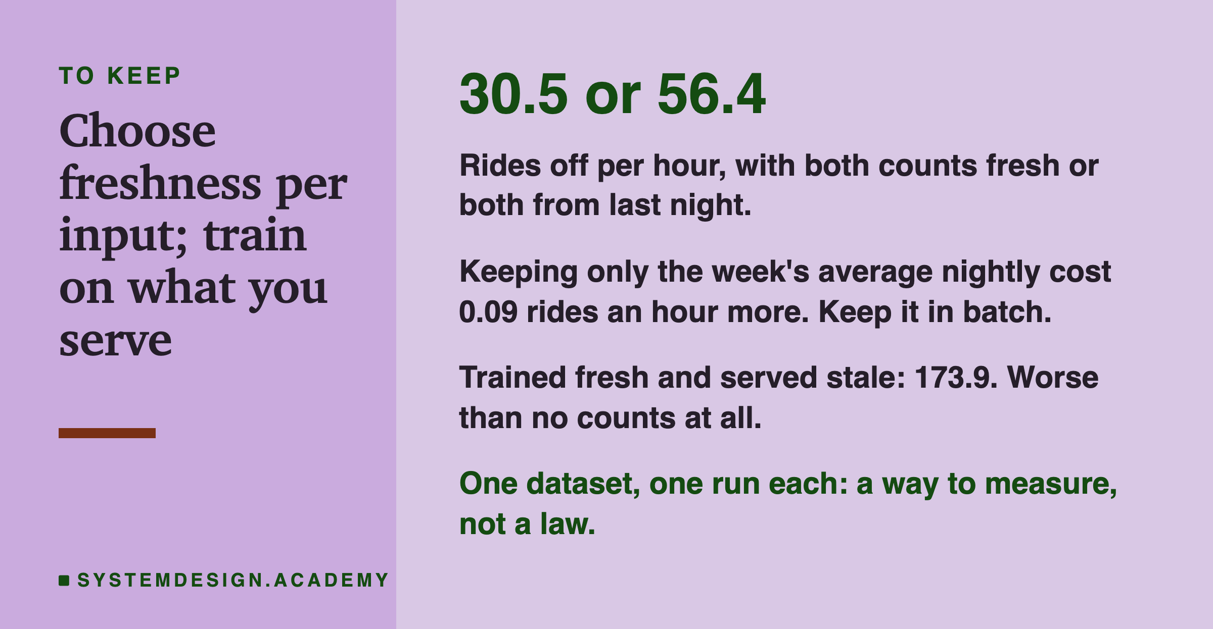
The card keeps three numbers from the lab. With both counts fresh the guesses were off by 30.5 rides an hour, and with both from last night by 56.4. Keeping only the week's average nightly cost 0.09 more. Training on fresh counts and serving stale ones cost the most: 173.9.
The next lesson in this chapter is about data ingestion pipelines. It covers how records get from where they are made into the log or the lake that both kinds of job read from.
Knowledge Check
Knowledge Check
4 questions - Score 80% to pass
The split design took the last-hour count from the stream and the 7-day count from the nightly job, and scored 30.6 against 30.5 for streaming both. What does that show?
The skew design was trained on fresh counts and served the nightly ones. Why did it score 173.9, worse than the calendar alone?
Two versions of the 7-day count, one working on clock hours and one on the rows a job receives, disagreed on 690 test hours. What made them differ?
What does exactly-once do that at-least-once does not?