Let me start in a classroom.

A teacher has a pile of tests to mark. Most students wrote full answers. One sheet is almost empty. Maybe the student joined the class last week and has not learned the topic yet. Maybe the student wrote a full page, and the page got lost on the way to the teacher's desk. Either way, the end-of-term ranking needs a mark for every student, so the teacher must write something in the book.

What mark should the empty sheet get? There are only a few sensible choices. A zero says "this student knows nothing", which is unfair if the page was lost. The class average says "this student is ordinary", which may or may not be true. A special mark, like "no paper", says "I do not know", and lets the teacher treat that student differently later.

None of these choices is obviously right. And the choice matters most when many sheets are blank at once.

Machine learning systems face the same question every day, many thousands of times. In this lesson I measure the choices on real data from a real shop.

This lesson uses the same shop, the same customers and the same question as the rest of the chapter. If any of that is new, please read what a feature is first. That lesson built six simple features from each customer's history: recency, frequency, money, return share, tenure and products. The question is always the same: at the start of a month, will this customer buy something in the next 30 days?

The lesson on feature freshness found something I promised to come back to. When the feature job runs 30 days late, 716 of the 26,851 test customers have no feature row at all. They are real customers who first appeared in the shop during those 30 days, so the job never saw them. That lesson simply left their features empty and moved on.

This lesson asks the question that lesson skipped. When a customer's features are missing at the moment the model is asked, what should the service put there instead? And does it matter how the model was trained?

Please read this slide slowly if any word is new. Every slide after it uses these words.

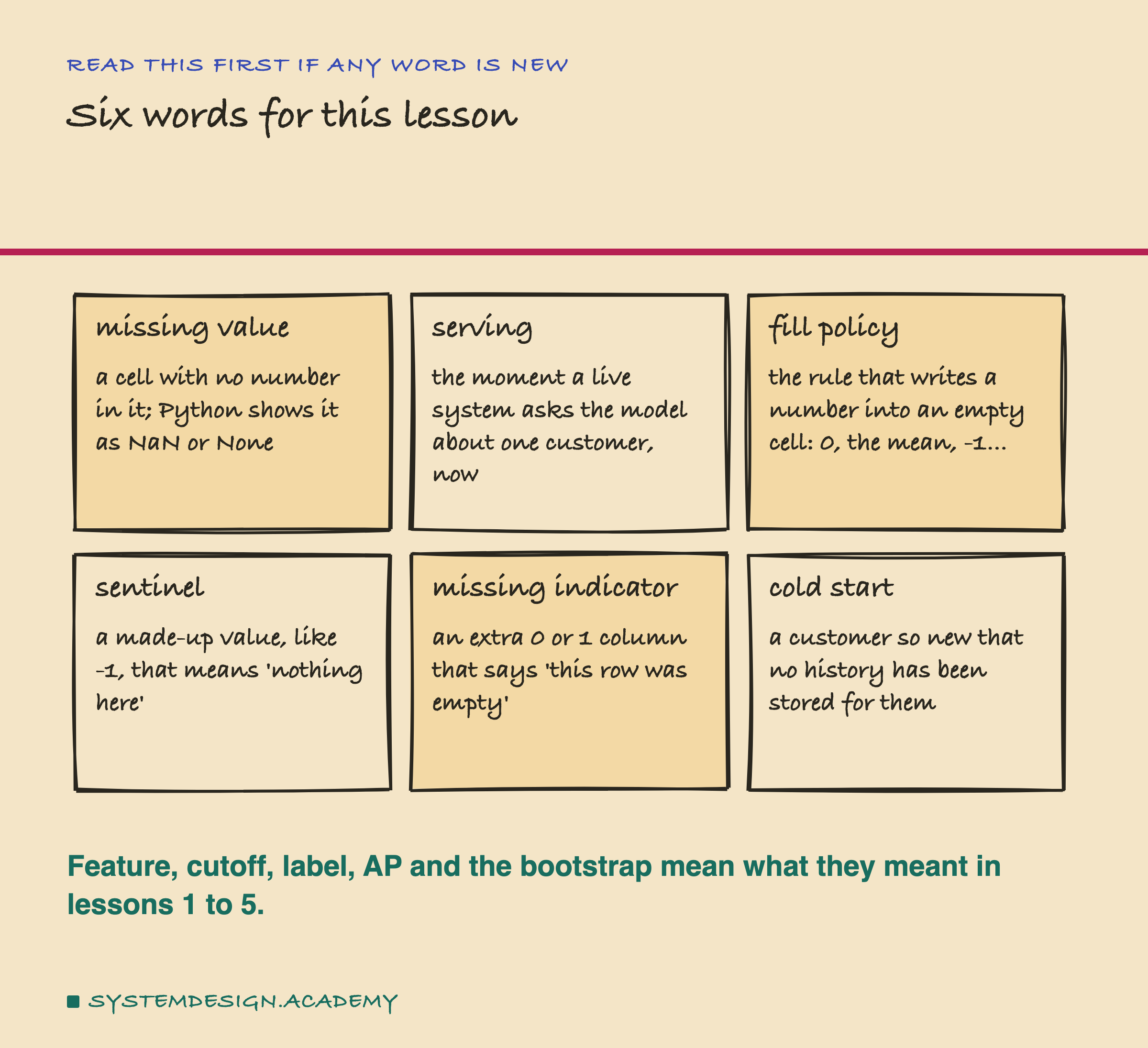
A missing value is a cell in a table that has no number in it. In Python you usually see it as NaN, short for "not a number", or as None. Think of the empty answer sheet.

Serving is the moment a live system asks the model about one customer, right now. Training happens once, at night, on old data. Serving happens all day, one request at a time.

A fill policy is the rule that writes a number into an empty cell before the model sees it. The common rules are these. Leave it as NaN. Write 0. Write the mean, the average of the column over the training rows. Write the median, the middle value when the column is sorted. Or write a sentinel: a made-up value, like -1, that a real row never has, so it means "nothing here".

A missing indicator is an extra column that holds 1 when the row was empty and 0 when it was not. It lets the model see the gap itself, not only the number that filled it.

A cold start is a customer so new that the system has stored no history for them yet. A feature store is a system that keeps feature values ready for the model to read. Its online store answers one customer at a time during serving. A lookup is one such read.

Feature, cutoff, label, average precision (AP), seed and bootstrap mean what they meant in lessons 1 to 5. I explain the bootstrap again where it matters.

There are two very different reasons a lookup finds nothing, and this lesson measures both.

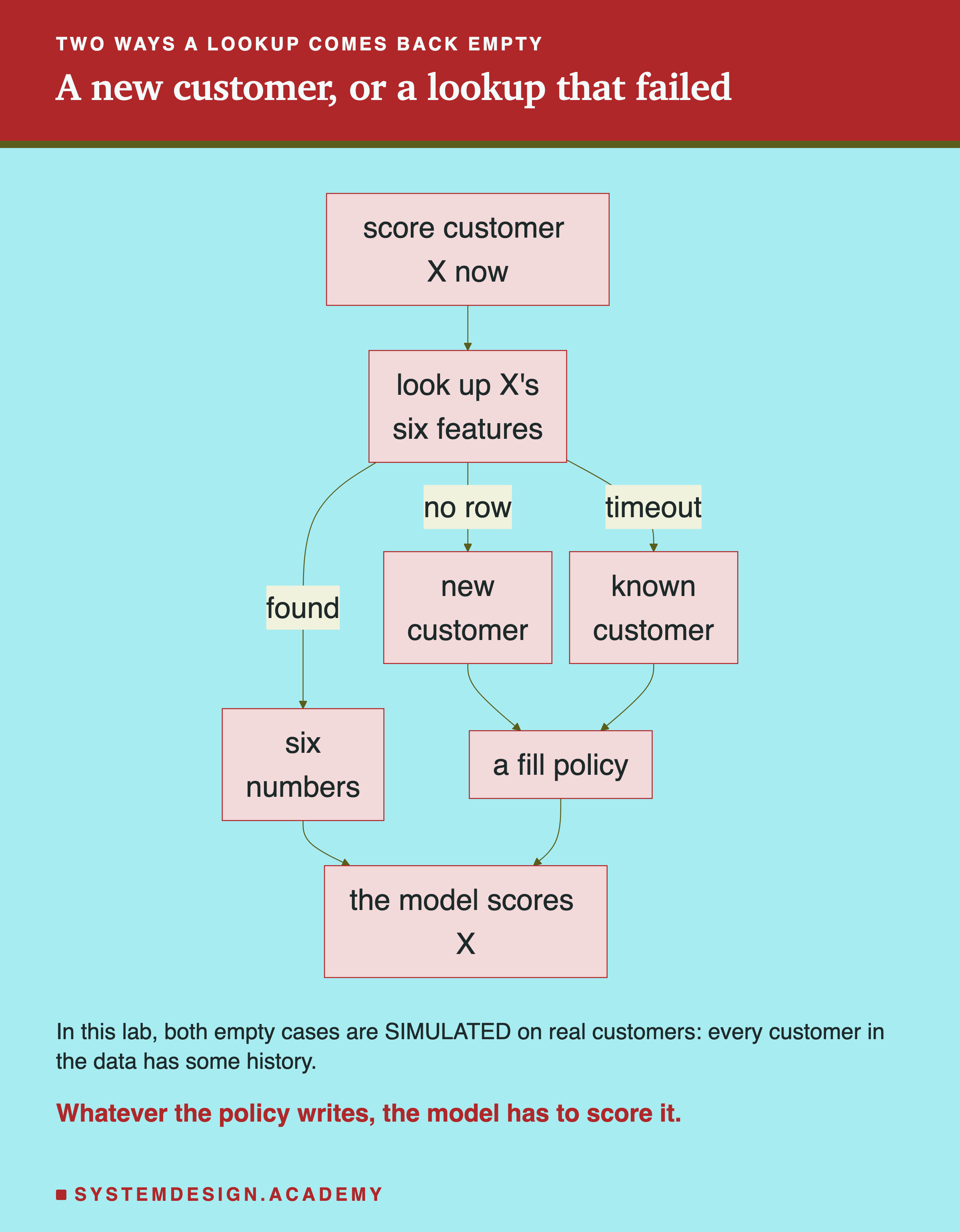
A new customer. Someone placed their first order this week. The nightly feature job has not run since, so the store has no row for them. This is a cold start, or close to one. Nothing went wrong; the data simply does not exist yet.

A failed lookup. A customer with two years of history asks for a page. The service asks the online store for their features, and the store does not answer in time. Or the key is missing because a pipeline run failed last night. The data exists somewhere, but not at this moment. The service has a few milliseconds to decide, so it falls back to something.

Here is an honest problem with my data. In this task, every customer in the test rows has at least one order before the cutoff, because that is how the rows are chosen. So a true cold start, with zero history, never appears. And no lookup ever fails, because the lab reads features from a table in memory.

So I make the gaps myself, on purpose. For new customers, I take the real customers who first appeared in the 30 days before the cutoff. They are the same 716 rows that lesson 3 found. I blank their features as if the row did not exist yet. For failed lookups, I blank the features of a random share of the other customers. Every gap in this lesson is simulated. The customers, their orders and whether they bought are all real.

Before measuring anything, I checked what real tools do when a value is missing. None of them stops with an error. Each one hands you something and carries on.

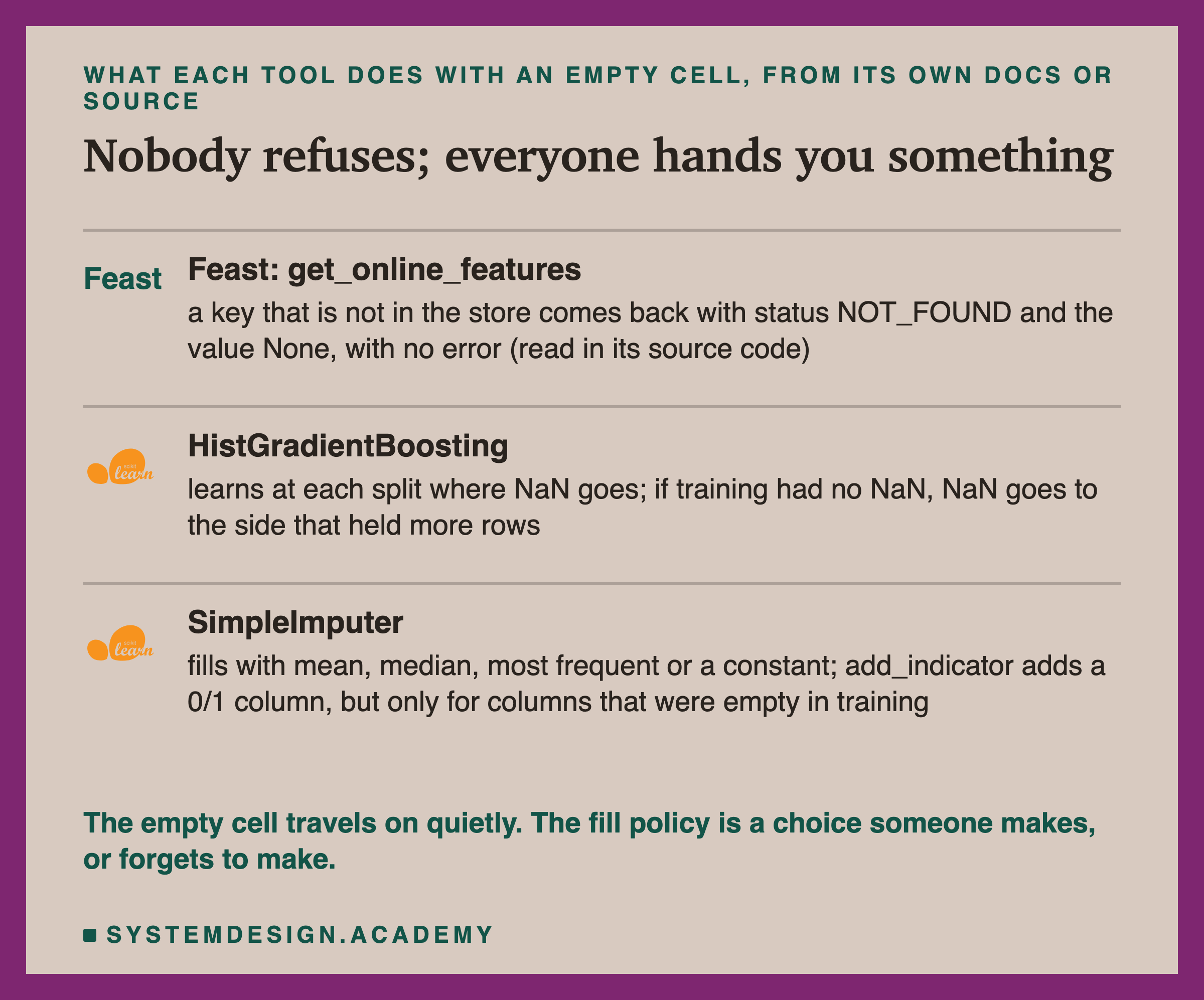
Feast is an open-source feature store, and a later lesson in this chapter uses it for real. Its documentation page on reading features does not say what happens to a missing key. So I read its source code, at commit 374f1d7a, on 1 October 2026, the day I wrote this lesson.

When a key is not found, Feast fills the answer with an empty value and marks it with a status called NOT_FOUND. Its own comment says this "could suggest that the feature values have not yet been ingested into feast or the ingestion failed". When you turn the answer into a Python dictionary with to_dict(), the empty value becomes None. So your code gets None for that customer, and no error. I have not run Feast in this lesson, so this is what the code says, not something I measured.

scikit-learn's HistGradientBoostingClassifier is the model of this whole chapter, and it accepts NaN directly. Its documentation says that during training, "the tree grower learns at each split point whether samples with missing values should go to the left or right child". It then adds the case that matters here. In its words: "If no missing values were encountered for a given feature during training, then samples with missing values are mapped to whichever child has the most samples." I also found that rule in the installed source code.

scikit-learn's SimpleImputer is a ready-made fill step. It can fill with the mean, the median, the most frequent value or a constant, and its constant is 0 for numbers by default. Its option adds missing-indicator columns. But its documentation warns: "If a feature has no missing values at fit/train time, the feature won't appear on the missing indicator even if there are missing values at transform/test time." Keep that sentence in mind for later. I recorded every quote in .

Here is one real new customer, number 12498, at the cutoff 1 November 2011. They first ordered 18.604 days before the cutoff, made one purchase of £247.25 across 13 products, and did buy again in the next 30 days.

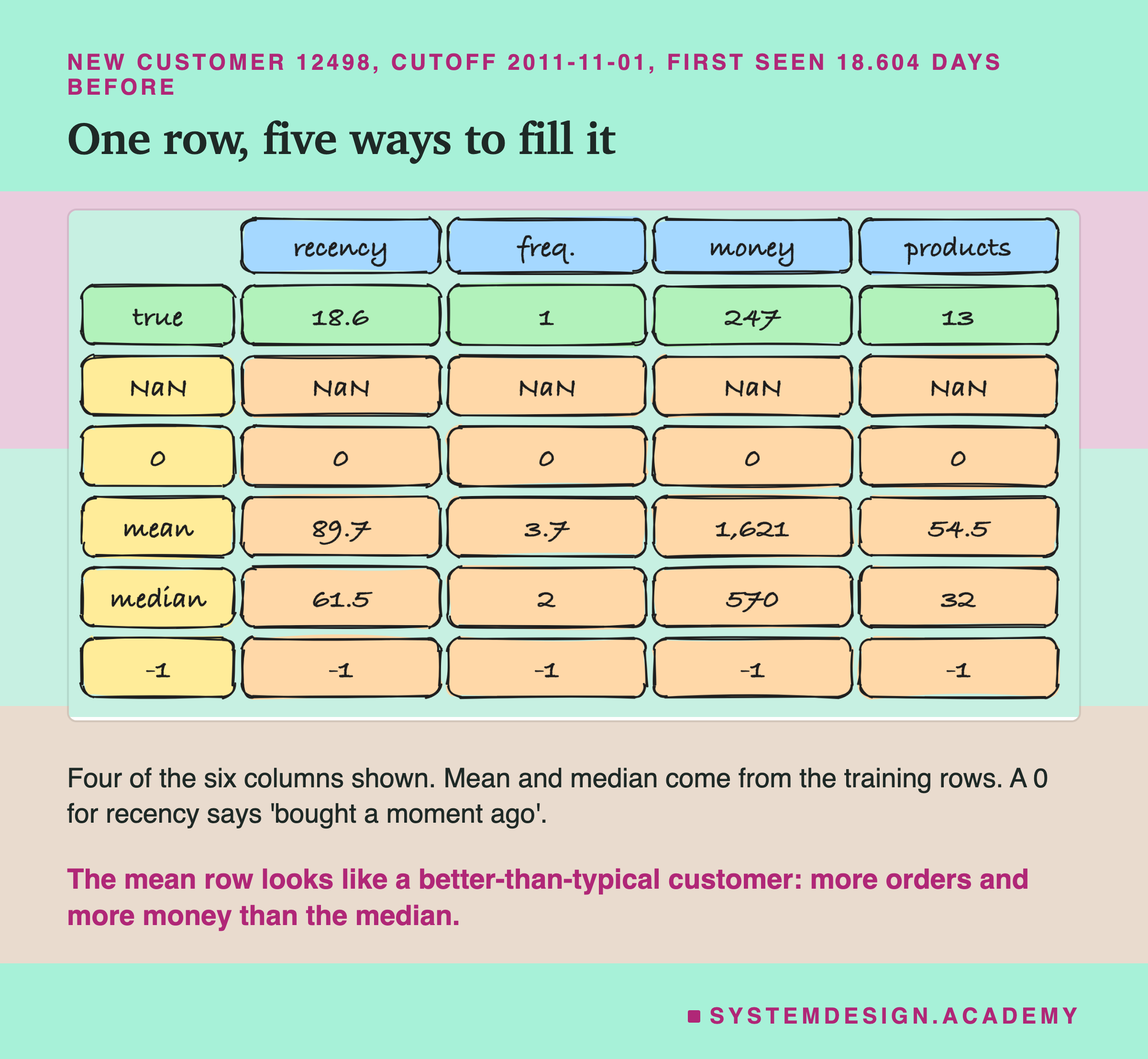
Now pretend their row has not been written yet. What does each fill policy put in its place?

NaN leaves every cell empty, and the model decides what an empty cell means. Zero writes 0 everywhere. Look at what that says: recency 0 means "bought a moment ago", and frequency 0 means "never bought". Those two cells contradict each other. Each value alone does occur in training. Some customers have 0 orders and 0 products. And a recency of 0 lands in the same group, or bin, as real recencies up to a few hours. But no real customer has all of them at once. -1 is the same kind of story, with a value below every real recency.

The mean row writes recency 89.7 days, frequency 3.7 orders, money £1,621 and products 54.5. The median row writes 61.5 days, 2 orders, £570 and 32 products. Those two look similar in words, "an average customer", but they are not. The mean row is a much better customer than the median row: almost twice the orders and almost three times the money. A later slide shows why, and why it mattered a lot.

One thing is true of every policy here. All six cells are filled the same way for every customer whose row is missing. So all of those customers get exactly the same row, and therefore exactly the same score.

Here is where the fill sits in a live service.

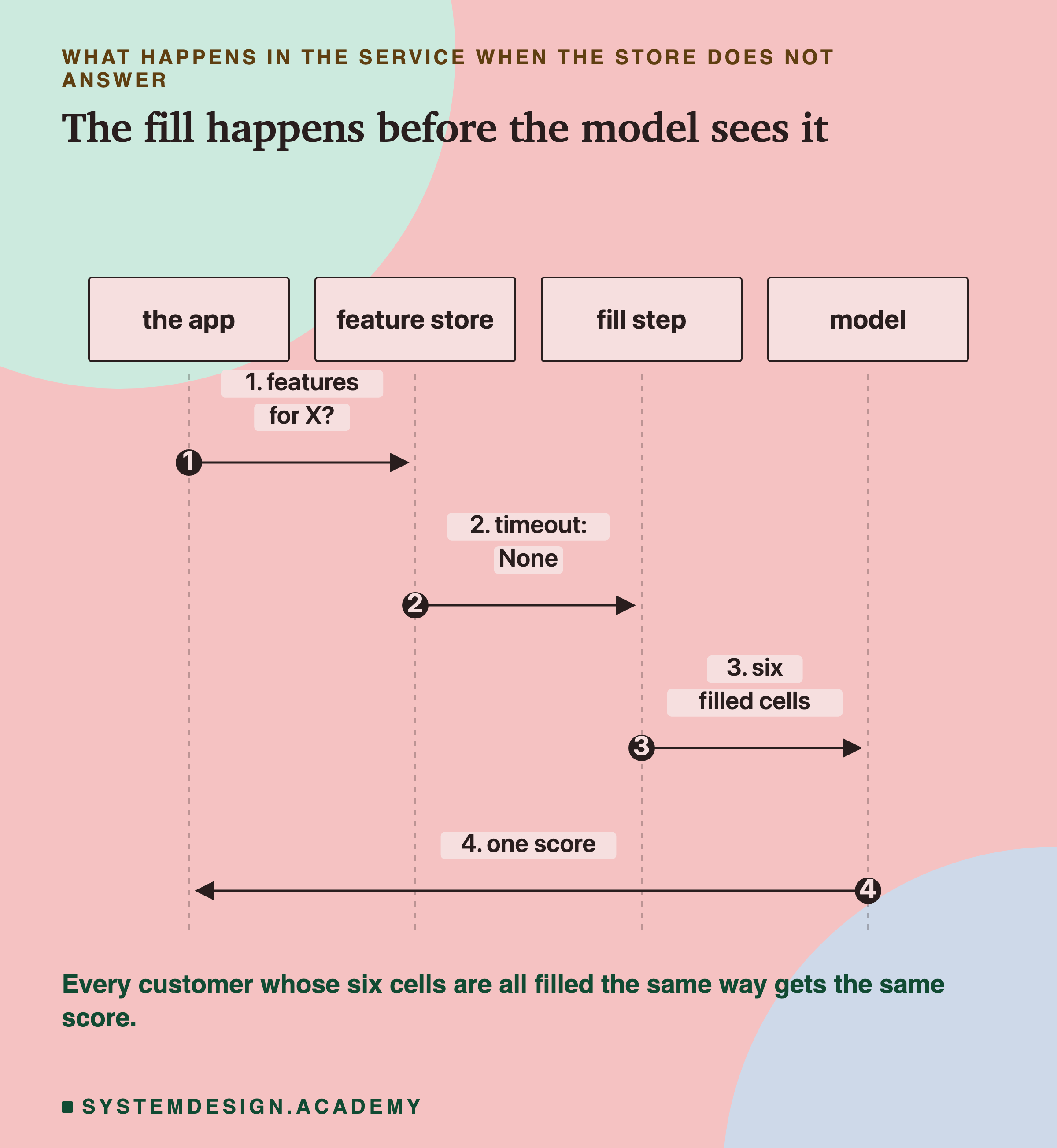
The app asks the store. The store fails, or finds no key, and returns None. A small piece of code, the fill step, turns that into numbers. The model scores the numbers and never learns that anything went wrong.

This matters for the measurement. A model ranks customers, and AP measures how well buyers are ranked above non-buyers. If 5,000 customers all get the identical score, the model cannot rank them against each other at all. The only thing the fill policy controls is where that block of identical scores sits among everyone else: high, low or in the middle.

So I expected the fill policy to matter mainly through that one position. The lab measures how much.

I wrote the lab's design into the docstring of scripts/labs/features/missing_at_serving.py before it first ran. Two small smoke tests ran before the full run, only to test the code, and both printed a few numbers from the first seeds. I changed nothing in the design after them, and the docstring says so.

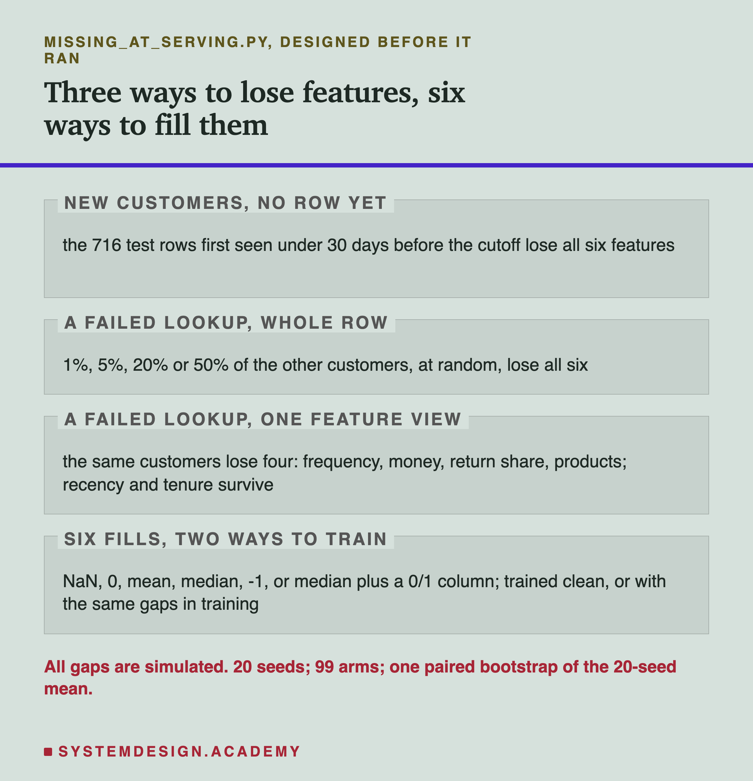
Three kinds of gap. First, new customers: all six features blanked for the 716 test rows whose first order was less than 30 days before the cutoff. Second, a whole-row lookup failure: 1, 5, 20 or 50 percent of the other 26,135 test rows, chosen at random within each month, lose all six features.

Third, a feature view failure. A feature view is a group of features that are stored and read together. Here the same customers lose only four features: frequency, money, return share and products. Recency and tenure survive, as if they came from a separate lookup that did answer. I added this third kind on purpose. With all six features gone, every failed customer gets the same score. The third kind is the only one where the failed group can still be ranked.

Six fills and two ways to train. A clean model is trained on true features, exactly lesson 1's model, and is then given the gaps only at serving. This is called the train/serve mismatch: training never saw an empty cell, but serving does. A model trained with gaps gets the same kind of gaps injected into its training rows, at the same rate, filled the same way. The missing indicator only makes sense for the second kind, because in clean training that column is always 0 and no split can use it.

What is measured. Test AP and ROC-AUC per month, then averaged over the five test months, as in every lesson of this chapter. I measure them over all rows, and over the failed rows alone. I also record where the block of identical scores lands. And I count how many failed customers move into or out of the . The top fifth is the 20 percent of each month with the highest scores, the group a shop would contact.

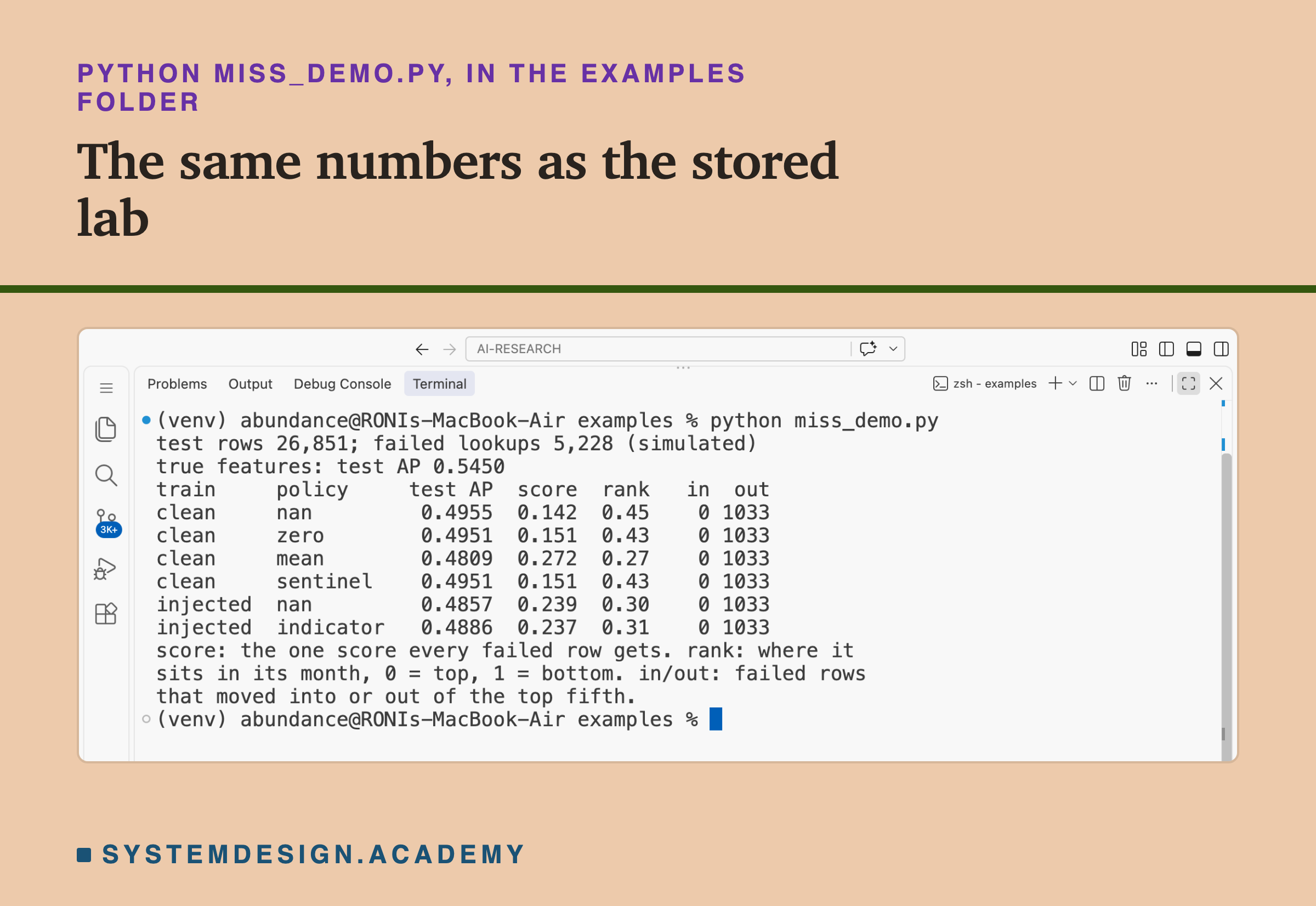
This is a real recording of the report script, miss_report.py, on the laptop where the lab ran. It refits every model the lab trained, reruns the bootstrap and checks every number.

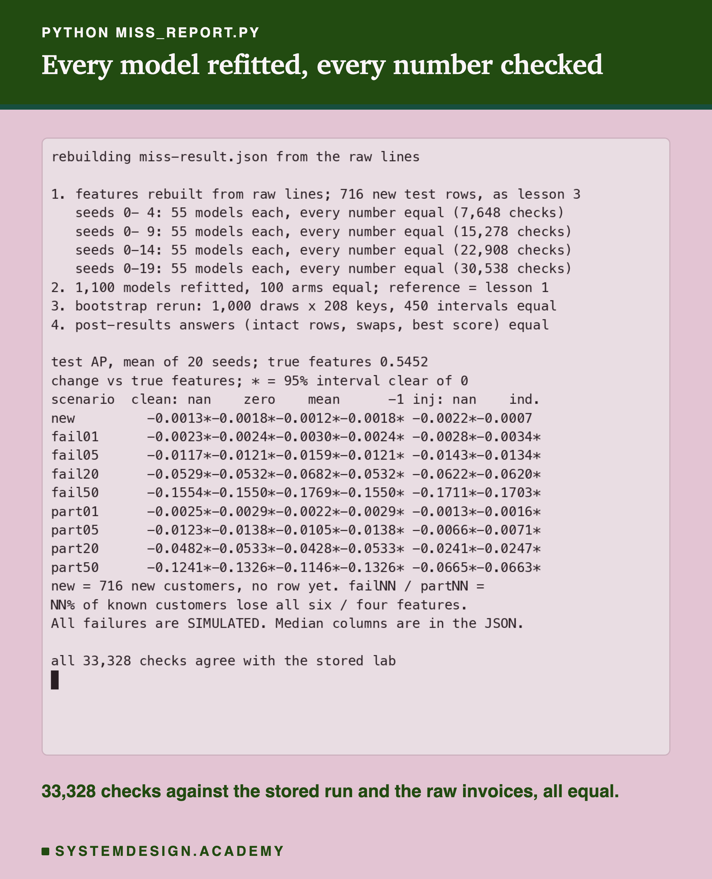
The report does not reuse the lab's code for the parts that matter. It rebuilds lesson 1's features from the raw invoice lines with its own groupby and requires them to match. It draws the failed customers, fills the cells, and computes AP, the block score, the ranks and the top-fifth moves with its own code. Then it refits all 1,100 models with the same seeds and requires every stored number to come back. It also checks that the clean model with true features equals lesson 1's model on all 20 seeds, and that its 716 new rows are lesson 3's 716. If anything disagrees, it stops with an error.

Here is the main result. The clean model with true features scored a mean test AP of 0.5452 over 20 seeds.

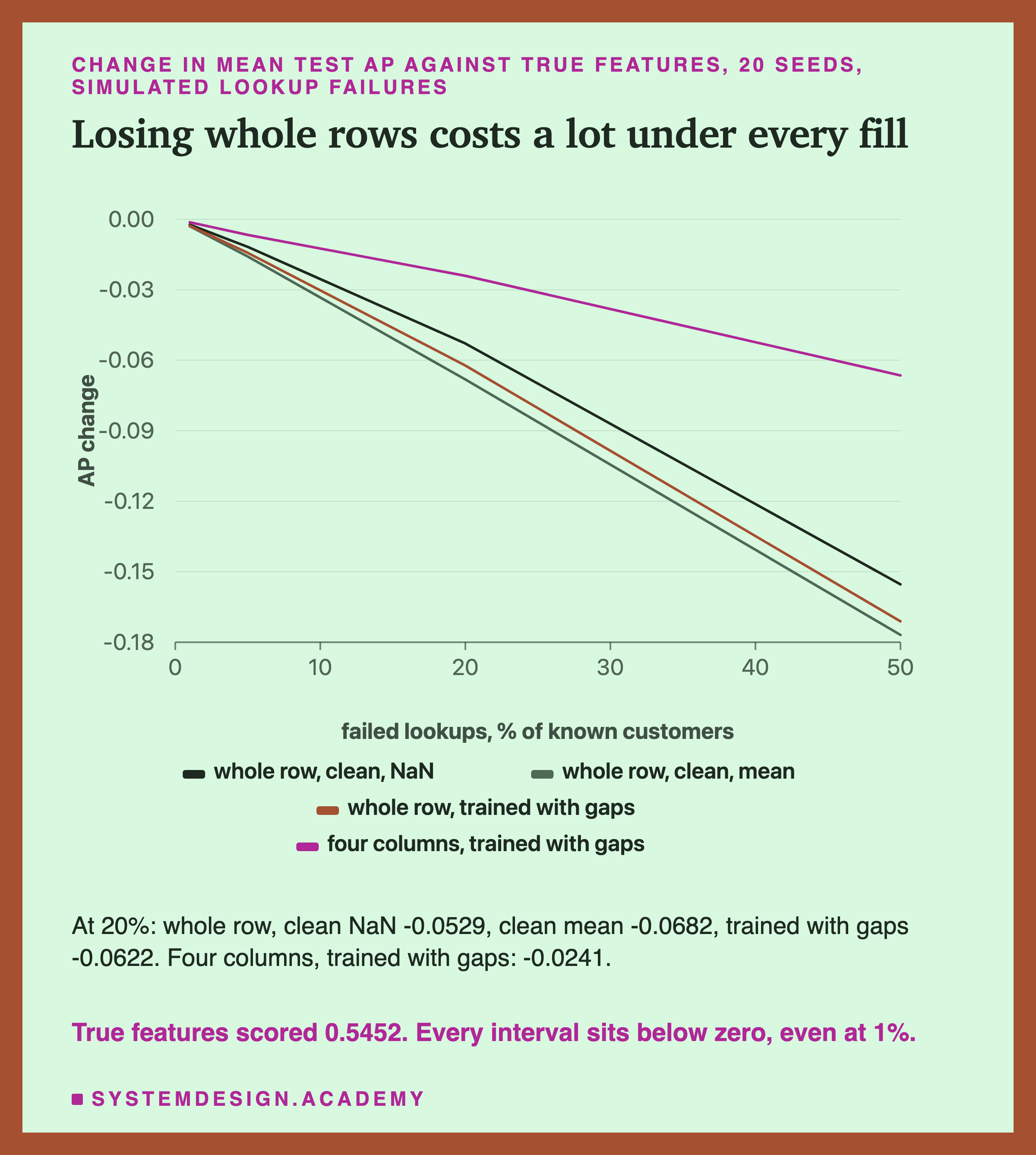
When a customer loses all six features, every fill costs real ranking, and the cost grows with the share that fails. At 20 percent failed, test AP fell by 0.0529 with NaN on the clean model. It fell by 0.0682 with mean fill on the clean model, and by 0.0622 with a model trained with the gaps. At 50 percent the losses were 0.1554, 0.1769 and 0.1711. From 5 percent up, all 20 seeds were below the true-feature score in every failed-lookup arm. At 1 percent, 16 to 20 of the 20 seeds were below it for models trained with gaps. Every 95% interval was below zero.

Even 1 percent cost something measurable. With NaN on the clean model, AP fell by 0.0023, interval -0.0027 to -0.0019. I had guessed, before the run, that 1 percent would be too small to see. I was wrong. Those 261 failed rows included, on average over the 20 seeds, 53 customers who sat in the top fifth with true features, and about 27 of them bought.

When only four columns fail and recency survives, the cost is much smaller, if the model was trained with gaps. At 20 percent, the four-column failure cost 0.0482 on the clean model with NaN, and 0.0241 on the model trained with gaps. Training with the gaps halved the loss. A later slide shows that the same training made whole-row failures worse.

I measured two kinds of luck, as in every lesson of this chapter.

Luck in training. With more than 10,000 training rows, this model turns on early stopping by itself and keeps 10 percent of the training rows aside, chosen at random. The seed moves that choice. Here the seed also moves which customers fail. So every number is a mean over 20 runs.

Luck in which customers were tested. A bootstrap draws the test customers again at random, within each month, with repeats allowed, and recomputes the score. I did it 1,000 times. In each draw I recomputed the AP of every arm for all 20 seeds and averaged them, so the interval covers both kinds of luck at once. The same draw is used for every arm, which is what paired means. The middle 95 percent of the 1,000 differences is the 95% interval. I call a difference measurable only when its interval sits entirely on one side of zero; otherwise I say it cannot be told apart from zero.

One correction, made after the run and labelled in the lab. At 1 percent, the failed group has only about 52 customers per month. In 191 of the 1,000 draws, some seed's month drew no buyer from that group, so AP inside the group was undefined. My first code reported "cannot be told apart from zero" for those intervals, which was wrong. They are now marked "undefined", recomputed from the stored draws. No overall-AP interval was affected.

Why do the fills differ at all, if they all give the failed customers one shared score? Because they put that score in different places.

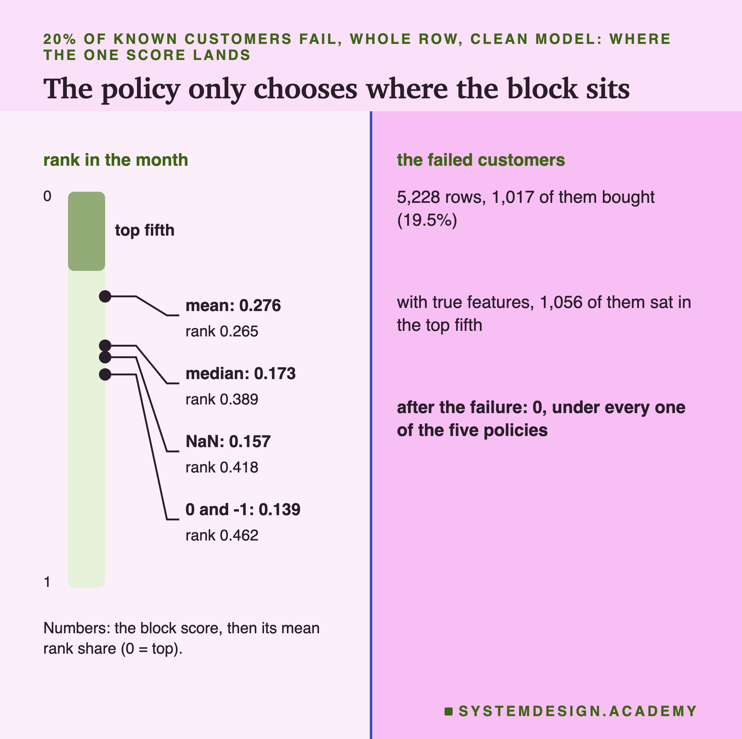
At 20 percent, 5,228 test rows fail. With true features, 1,056 of them sat in the top fifth of their month. After the failure, under all five fills on the clean model, none did. The shared score never reached the top fifth.

Look at where each block lands. Mean fill gave every failed customer a score of 0.276, high enough to sit at about a quarter of the way down the ranking. NaN gave 0.157, a little above the middle. Zero and -1 gave exactly the same score, 0.139, in all 20 seeds.

I checked why, after a review asked. Before it builds any tree, this model sorts each column into at most 255 groups called bins, and the trees only ever see the bin. In all 20 seeds, 0 and -1 fell into the same bin in all six columns. So the model cannot tell them apart. A straight-line model would read 0 and -1 as different numbers.

Only 19.5 percent of the failed customers bought, about the same as everyone else. So putting them all high, as mean fill did, pushed a large crowd of ordinary customers above many real buyers. That is why mean fill was the worst whole-row policy on the clean model, at every rate.

The figure above is about the failed customers against everyone else. What about the failed customers against each other?

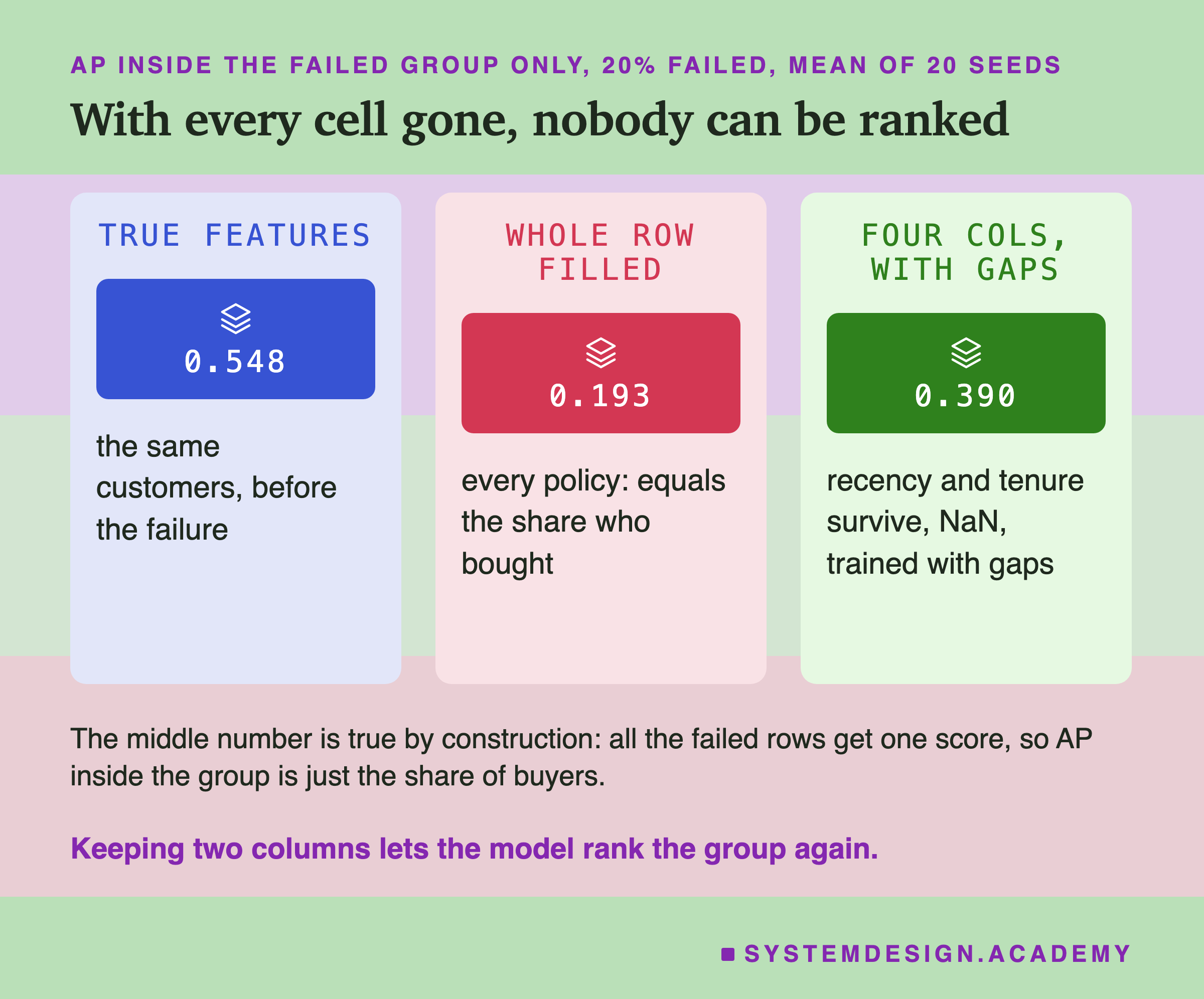
With true features, the model ranked those same 5,228 customers with an AP of 0.548. After a whole-row failure, AP inside the group is 0.193 under every fill, the mean over the five months. Please do not read 0.193 as a finding. It is true by construction. When every row in a group has the same score, AP can only equal the share of buyers in that group, month by month. That is why 0.193 differs a little from the 19.5 percent above, which counts all five months together. The lab checks this equality in every run, and it is there to show what is lost, not to compare fills.

The four-column failure is different. Recency and tenure still vary between customers, so the model can still rank them. Trained with gaps and NaN, it reached 0.390 inside the group. On the clean model the same group scored between 0.246 and 0.317, depending on the fill. So keeping even two columns alive gave back a large part of the ranking that a whole-row failure destroys.

Mean fill was the worst whole-row policy on the clean model. It sounds like the safest choice, "assume an average customer", so why?

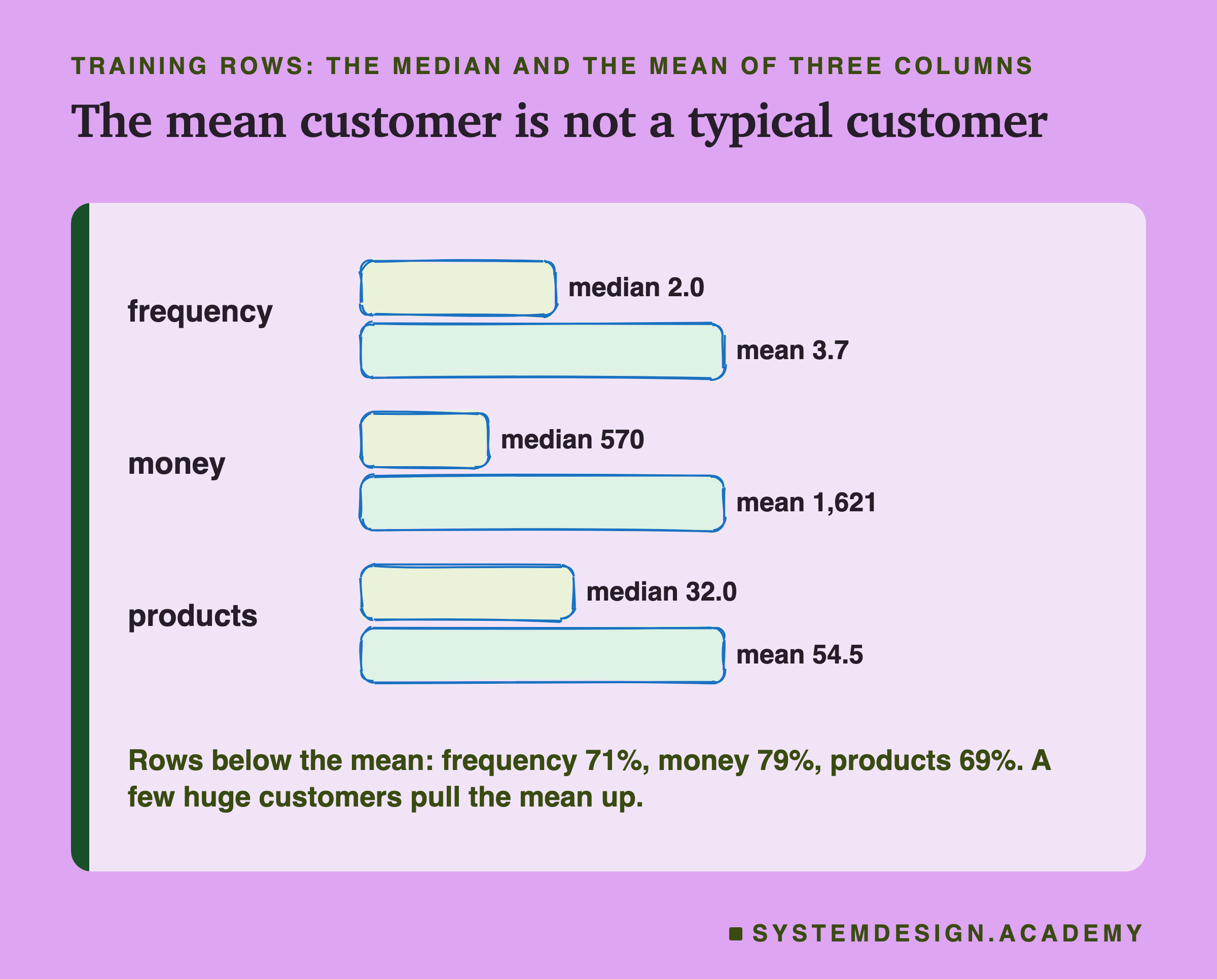
This part was asked after I saw the results, and the lab labels it so. In the training rows, the median customer made 2 orders and spent £570. The mean customer made 3.7 orders and spent £1,621. That gap comes from a few very large customers. They pull the mean far above the middle. In fact 71 percent of rows have fewer orders than the mean, and 79 percent spent less than the mean.

So "the mean" is not a typical customer at all. It describes a customer better than about three quarters of the shop. The model, quite reasonably, scored such a customer high: 0.276 on average, against 0.173 for the median row. When thousands of failed customers all got that flattering row, they crowded out real buyers near the top.

The lesson I take is simple. For columns like counts and money, which have a long tail of huge values, the median is a far more honest "average" than the mean. Here the median fill cost about the same as NaN.

AP is an average over thousands of customers. A shop that contacts its top fifth sees something more direct: which people are on the list.

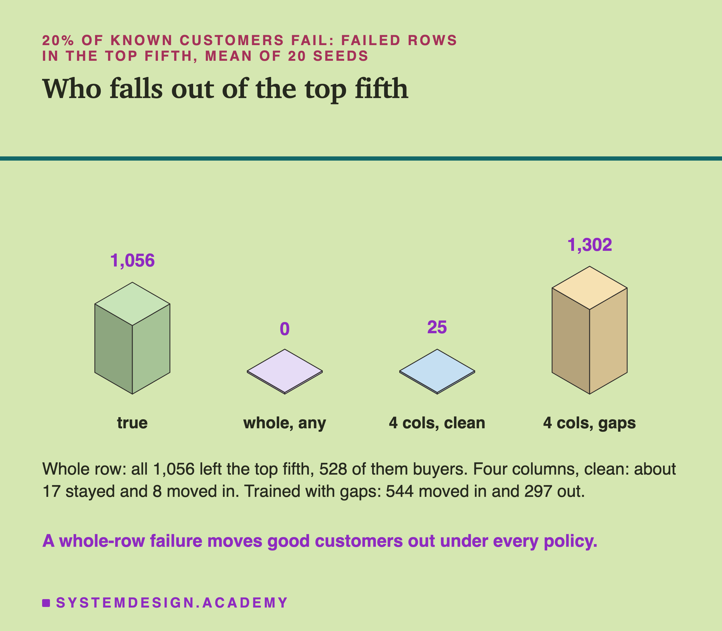
Take a whole-row failure at 20 percent. All 1,056 failed customers who belonged in the top fifth fell out of it, under every fill and both ways of training. 528 of them, half, were buyers. They simply vanish from the contact list.

With the four-column failure on the clean model, about 25 failed customers ended up in the top fifth. That is about 17 who were already there, and 8 who moved in. 1,039 moved out. The clean model saw empty cells it had never trained on, followed the "bigger side" rule at every split, and pushed nearly all of them down.

Trained with gaps, the four-column picture changed completely: 1,302 failed customers ended up in the top fifth, more than the 1,056 who belonged there. 544 moved in and 297 moved out. Of the 544 who moved in, 120 bought; of the 297 who moved out, 117 bought. So the model trained with gaps did not just keep the ranking; it shuffled it, and lifted more failed customers than true features would have. One possible reason, which I did not test: to a model that learned from gaps, a customer with a recent order and an unknown history looks promising.

Before the run I expected training with gaps to win everywhere. A model that has seen empty cells should know what they mean. It did not win everywhere.

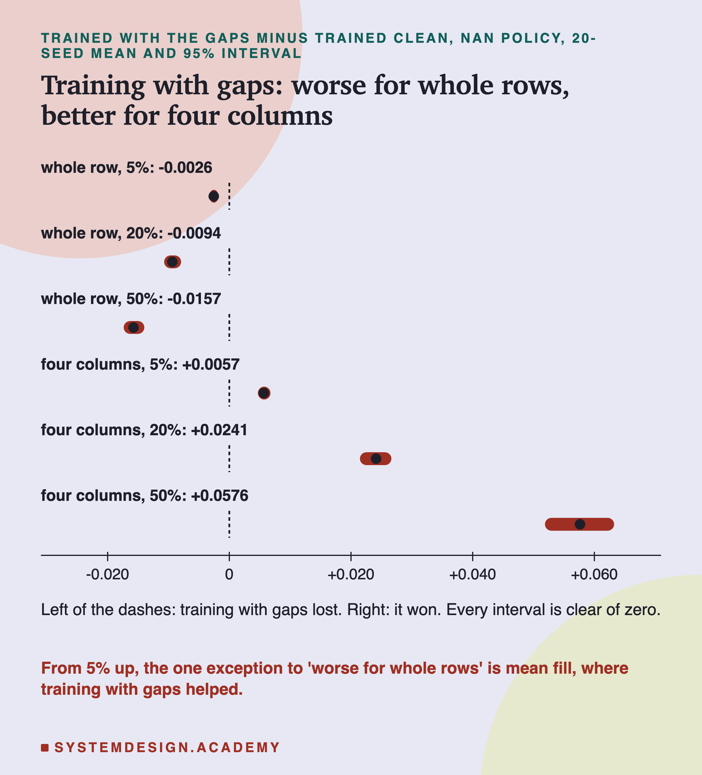
For whole-row failures from 5 percent up, training with gaps was worse than training clean, with every interval below zero. At 20 percent with NaN, it cost an extra 0.0094. For four-column failures, training with gaps was better at every rate, and by a lot: 0.0241 at 20 percent and 0.0576 at 50 percent.

There is one exception on the whole-row side from 5 percent up. With mean fill, training with gaps helped, by 0.0056 at 20 percent. At 1 percent, the gap-minus-clean intervals for mean and median fill cross zero. That fits the last slides: the clean model scored the mean row far too high, and a model trained with gaps learned to score it lower.

One more finding. Trained with gaps, median fill and median plus the missing indicator gave identical scores on every one of the 26,851 test rows. That held in all 20 seeds, for both new customers and the 20 percent whole-row failure.

After a review asked, I counted the splits in every tree. The indicator column was there, and it held 1 for exactly the blanked training rows. But in all 20 seeds of both scenarios, no tree ever split on it. Both models had the same number of splits on every other column, and the same number of trees.

For the 20 percent failure, one reason a split gains nothing: blanked training customers bought at 23.8 percent, against 23.4 percent for all training customers. For new customers that reason does not hold, 18.8 against 23.4 percent, so there I can report the count but not the cause. In the four-column failure, the same indicator was used in 22 to 34 splits per model, and every test score differed.

Why would training with gaps hurt whole-row failures? I asked this after the results, and the lab labels the answer as a post-results question.

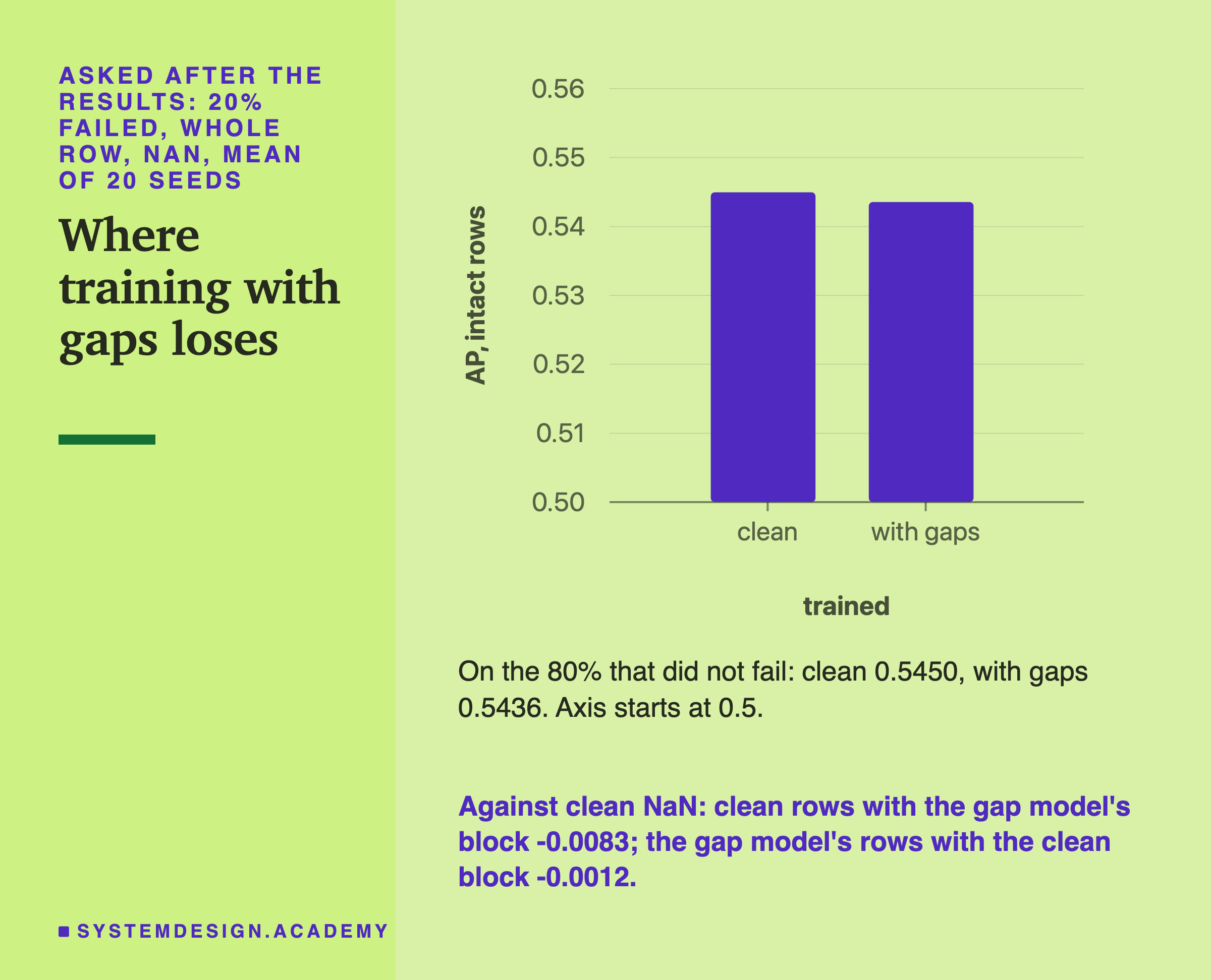
There are two possible causes. The model trained with gaps learned from fewer complete rows, so it might rank the healthy customers worse. Or it might place the block of failed customers in a worse spot. So I swapped the parts. I took the clean model's scores for the healthy rows and gave the failed rows the gap model's block score, and the other way round.

On the 80 percent that did not fail, the gap model was only a little worse: 0.5436 against 0.5450. Swapping in the gap model's block alone cost 0.0083 against clean NaN, interval -0.0095 to -0.0071. Swapping in its healthy-row scores alone cost 0.0012, interval -0.0018 to -0.0004. Most of the loss, then, came from where the block landed.

And why did it land badly? I measured this after a review asked, over the 20 seeds. On the intact test rows, both models were about equally calibrated. Calibration compares the average predicted chance with how often people really bought. Their mean predicted chance was 0.1886 for the clean model and 0.1891 for the gap model, against an actual buy rate of 0.1981.

But the gap model scored the blanked rows at 0.2385, almost exactly the 23.81 percent of blanked training customers who bought. In the test months, the failed customers bought only 19.45 percent of the time. Over all customers, the training months had a higher buy rate too: 23.4 percent against 19.7 percent. My reading, which fits these numbers but which I did not test directly: the model learned the right meaning of "empty", for the wrong months.

If the fill only chooses where the block sits, what is the best possible place? I asked this after the results too.

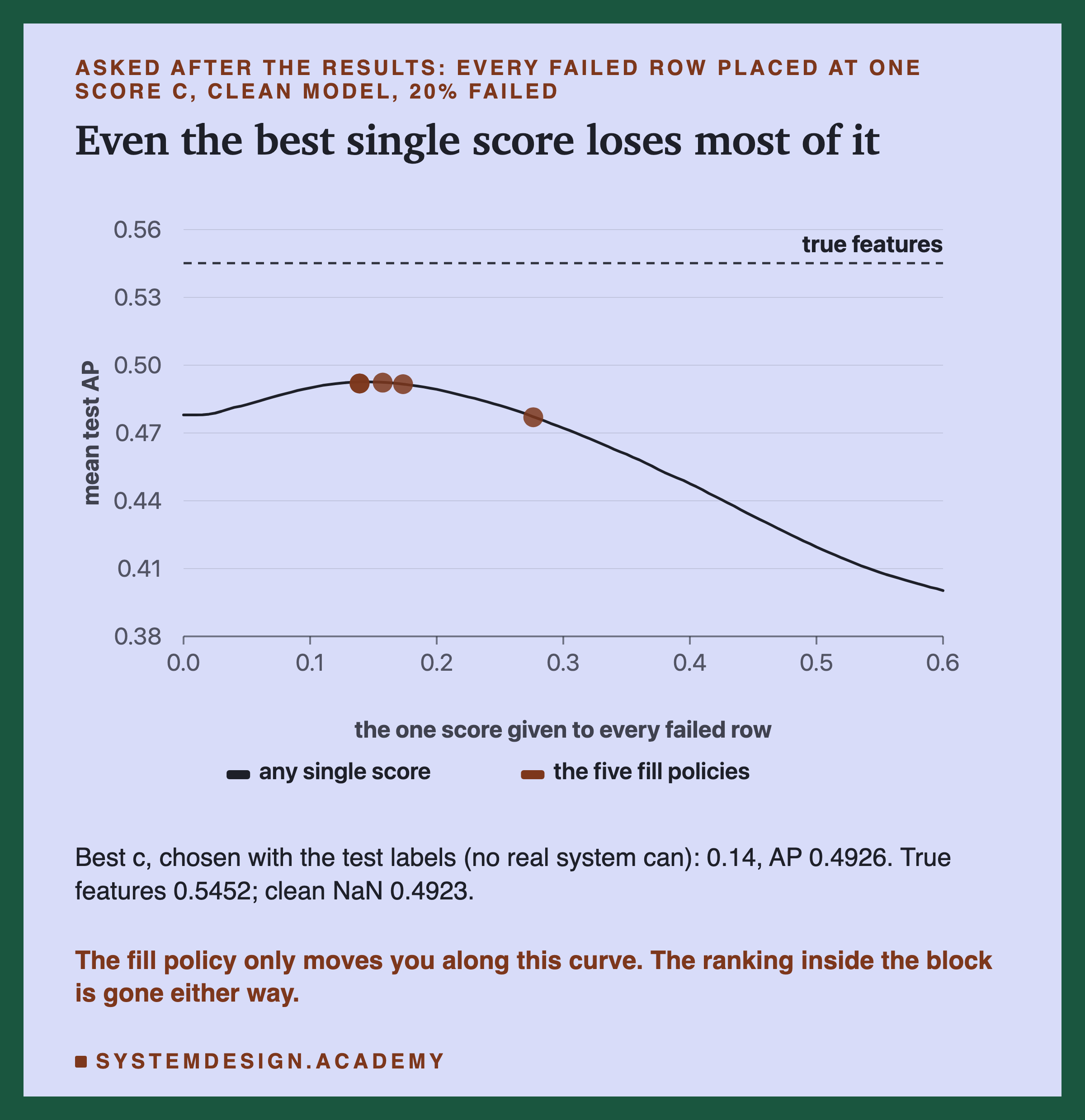
I gave every failed customer one score c, tried 121 values from 0 to 0.6, and kept the clean model's scores for everyone else. The best c, 0.14, reached a mean AP of 0.4926. That choice used the test labels, which no real system can see, so treat it only as an upper limit.

Two things stand out. First, the clean model with NaN reached 0.4923, only 0.0003 below that upper limit. In this lab, the "bigger side" rule happened to send the block almost exactly to the best place. I would not expect that luck to hold on other data.

This luck is also part of why training with gaps looked worse for whole rows, on the slide about training with gaps. Here the clean model happened to sit near the best place, so it was hard to beat. On other data, the clean model may not be so lucky.

Now the first kind of gap: the 716 new customers whose row does not exist yet.

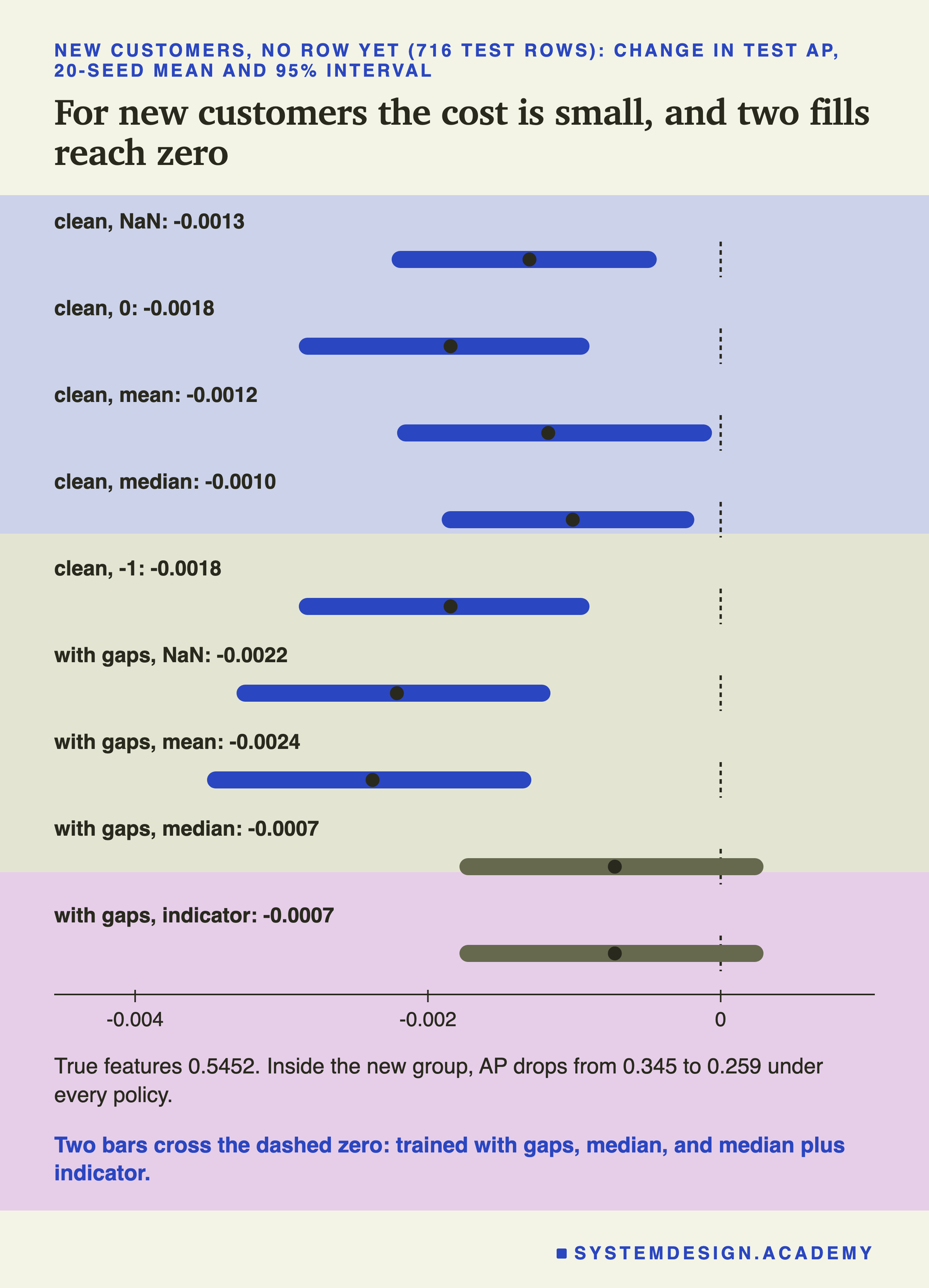
Overall, the cost is small, because 716 is only 2.7 percent of the test rows. Every fill on the clean model cost a measurable amount, from 0.0010 with the median to 0.0018 with 0 or -1. Trained with gaps, the median and the median plus indicator cost 0.0007, an amount that cannot be told apart from zero. The other gap-trained fills cost more, 0.0022 to 0.0025.

Inside the new group the loss is large. With their true short histories, the model ranked new customers with an AP of 0.345. With the row missing, every fill gives 0.259, which is just the share of them who bought, by construction.

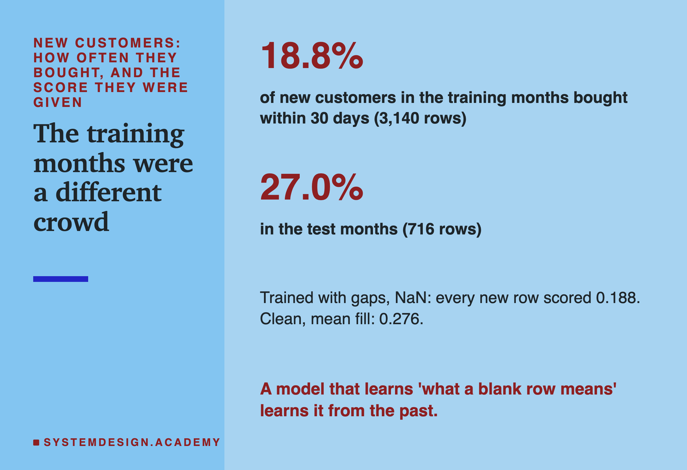
Here is a detail that I find more useful than the averages. In the training months, 18.8 percent of new customers bought within 30 days. In the test months, 27.0 percent did. A model trained with gaps learned that a blank row means "new customer, about 18.8 percent", and scored every new customer at 0.188. That was the right lesson from the past and the wrong number for the test months.

Meanwhile the clean model with mean fill scored new customers at 0.276, close to their real rate, by the accident of flattering means. So a policy can look good here for a bad reason. I would not choose mean fill because of this.

I wrote seven guesses into the lab before it ran. Here they are against the results, because a guess that was wrong teaches more than one that was right.

1. "At 1 percent, nothing can be told apart from zero." Wrong. Every arm lost measurably at 1 percent, because the few failed customers included many from the top fifth.

2. "NaN on the clean model lands in the lower half." Wrong. Its block landed at a rank of about 0.42, a little above the middle.

3. "Zero and -1 land high, because recency 0 looks like a fresh buyer." Wrong. They landed lowest of all, at about 0.46. One possible reason, not tested: frequency 0 and products 0 outweighed recency 0.

4. "Mean and median land in the middle." Half wrong. The median did; the mean landed high, for the reason on the mean slide.

5. "Training with gaps wins at 20 and 50 percent." Right for four-column failures, wrong for whole-row failures.

6. "New customers lose all ranking inside their group, and the overall cost is small." Right, and the first half is true by construction.

7. "The four-column failure keeps most of the group's ranking." Partly right. Trained with gaps it kept 0.390 of the 0.548, well above the 0.193 of a whole-row failure, but not most.

The full lab trains 55 models for each of 20 seeds. I wrote a small demo that does one slice of it. It uses the 20 percent whole-row failure and seed 0. It tries four fills on the clean model and two on a model trained with gaps.

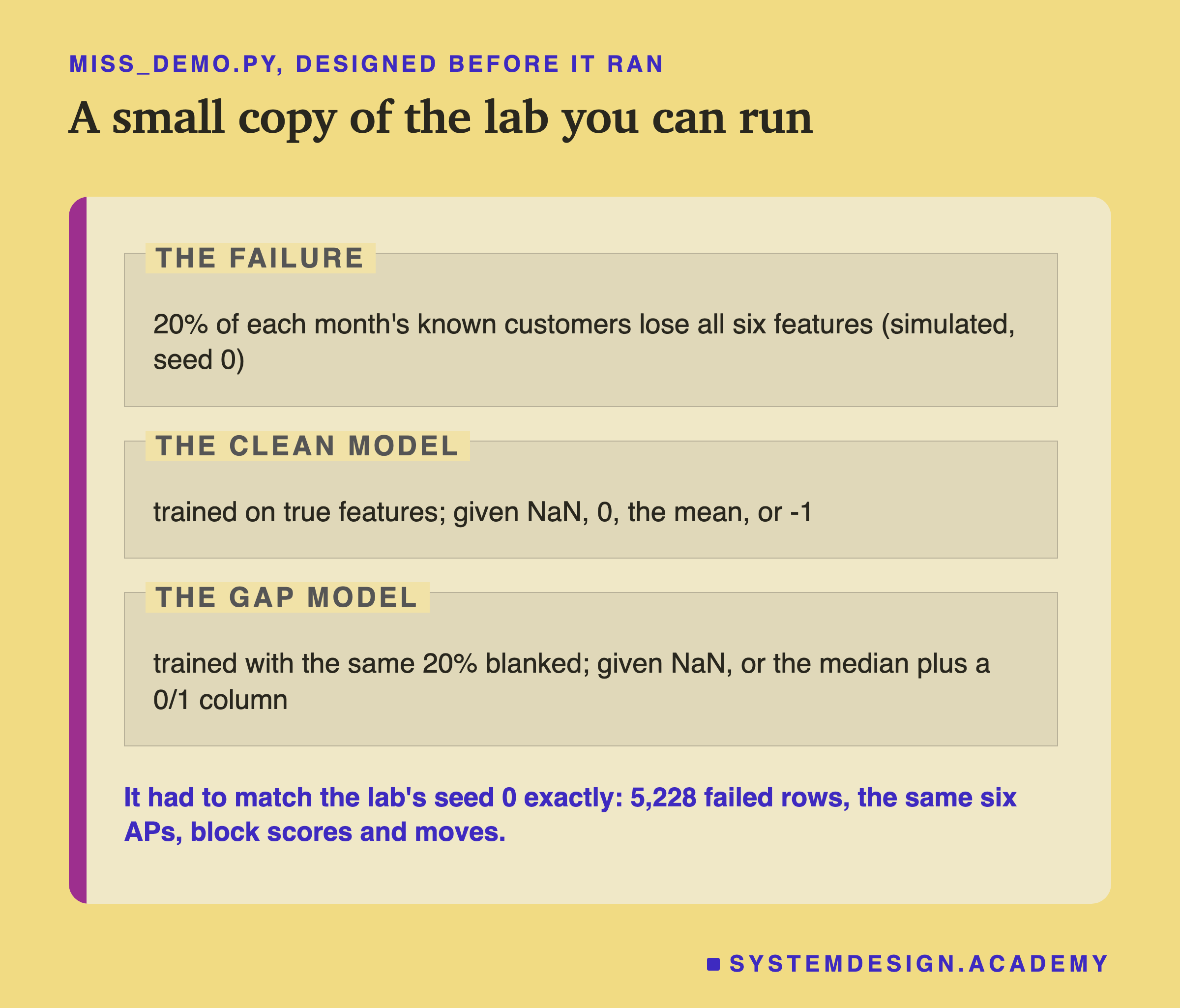
I wrote the demo's design into its docstring after the lab had run and before the demo first ran. Its code is shorter than the lab's and written separately, so it is also a second check of the lab's seed 0.

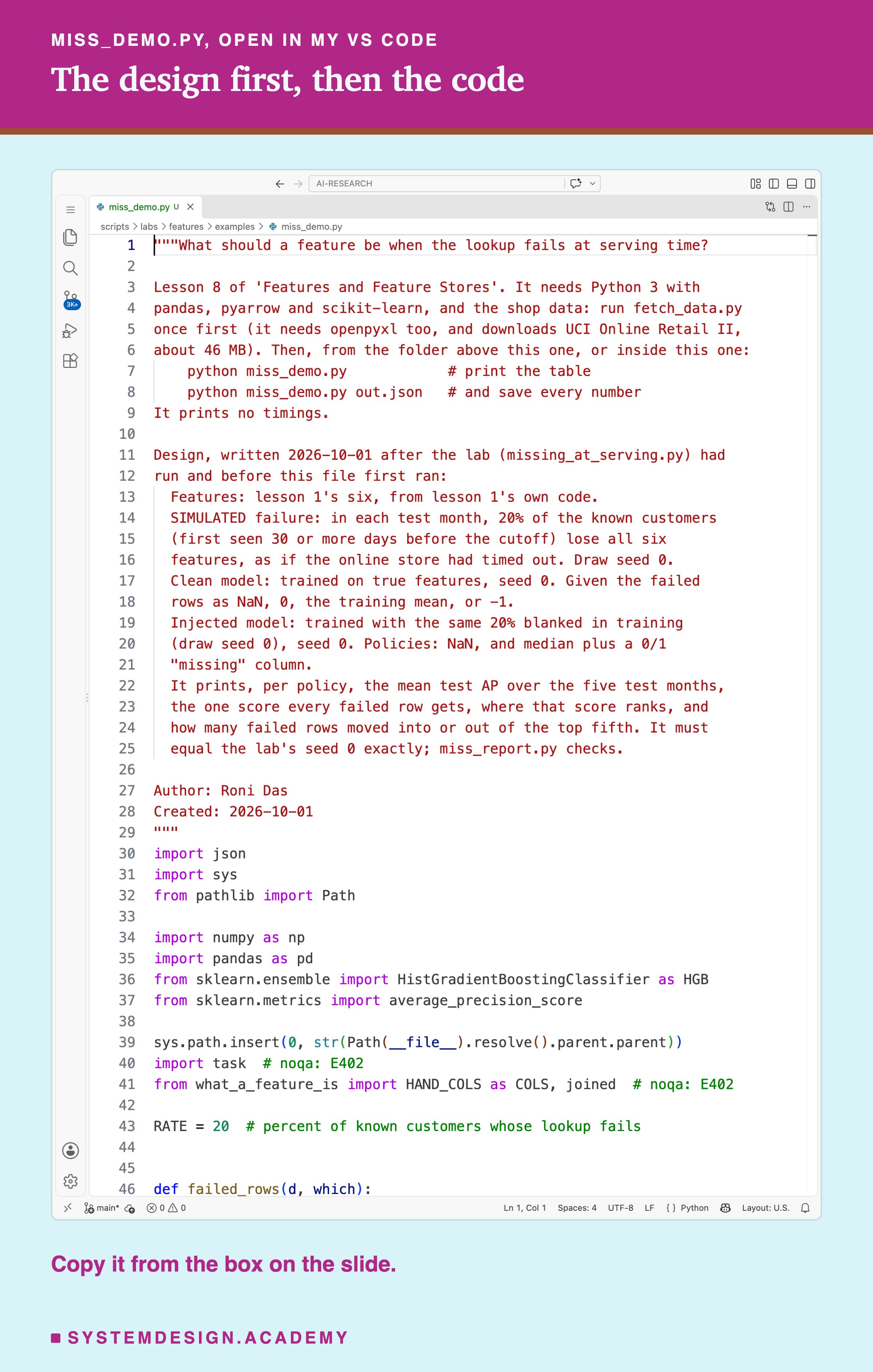
Before you run this lab. You need Python 3 with pandas, pyarrow and scikit-learn: pip install pandas pyarrow scikit-learn openpyxl. First run python fetch_data.py from the scripts/labs/features folder. It downloads the shop data once, about 46 MB, and writes one cleaned file.

The demo imports lesson 1's lab file, what_a_feature_is.py, from that same folder. It needs no GPU. I ran it with scikit-learn 1.9.1 and pandas 3.0.6 on a Mac. It finished well under a minute. Other programs were using the machine at the time, so I give no exact time. These libraries run on Windows and Linux too, but I have not checked the numbers there. Give it a file name, python miss_demo.py out.json, and it also saves every number. That is how results/miss-demo.json was made.

"""What should a feature be when the lookup fails at serving time?

Lesson 8 of 'Features and Feature Stores'. It needs Python 3 with
pandas, pyarrow and scikit-learn, and the shop data: run fetch_data.py
once first (it needs openpyxl too, and downloads UCI Online Retail II,
about 46 MB). Then, from the folder above this one, or inside this one:
    python miss_demo.py            # print the table
    python miss_demo.py out.json   # and save every number
It prints no timings.

Design, written 2026-10-01 after the lab (missing_at_serving.py) had
run and before this file first ran:
  Features: lesson 1's six, from lesson 1's own code.
  SIMULATED failure: in each test month, 20% of the known customers
  (first seen 30 or more days before the cutoff) lose all six
  features, as if the online store had timed out. Draw seed 0.
  Clean model: trained on true features, seed 0. Given the failed
  rows as NaN, 0, the training mean, or -1.
  Injected model: trained with the same 20% blanked in training
  (draw seed 0), seed 0. Policies: NaN, and median plus a 0/1
  "missing" column.
  It prints, per policy, the mean test AP over the five test months,
  the one score every failed row gets, where that score ranks, and
  how many failed rows moved into or out of the top fifth. It must
  equal the lab's seed 0 exactly; miss_report.py checks.

Author: Roni Das
Created: 2026-10-01
"""
import json
import sys
from pathlib import Path

import numpy as np
import pandas as pd
from sklearn.ensemble import HistGradientBoostingClassifier as HGB
from sklearn.metrics import average_precision_score

sys.path.insert(0, str(Path(__file__).resolve().parent.parent))
import task  # noqa: E402
from what_a_feature_is import HAND_COLS as COLS, joined  # noqa: E402

RATE = 20  # percent of known customers whose lookup fails


def failed_rows(d, which):
    """RATE% of each month's known customers, drawn at random."""
    rng = np.random.default_rng([0, RATE, which])
    known = (d["tenure_days"] >= 30).to_numpy()
    mask = np.zeros(len(d), dtype=bool)
    for _, idx in sorted(d.groupby("cutoff").indices.items()):
        k = idx[known[idx]]
        mask[rng.choice(k, int(round(RATE / 100 * len(k))), replace=False)] = True
    return mask


def fill(d, mask, policy, ref):
    """The six columns, failed rows filled by the policy."""
    x = d[COLS].astype(float).copy()
    value = {"nan": np.nan, "zero": 0.0, "sentinel": -1.0}
    for c in COLS:
        if policy in value:
            x.loc[mask, c] = value[policy]
        elif policy == "mean":
            x.loc[mask, c] = ref[c].mean()
        else:  # "indicator": the median, plus a 0/1 column
            x.loc[mask, c] = ref[c].median()
    x = x.to_numpy(float)
    if policy == "indicator":
        x = np.hstack([x, mask[:, None].astype(float)])
    return x


def per_month(d, p):
    d = d.assign(p=p)
    ap = d.groupby("cutoff")[["label", "p"]].apply(
        lambda g: average_precision_score(g["label"], g["p"])).mean()
    share = d.groupby("cutoff")["p"].rank(ascending=False, pct=True)
    return ap, share.to_numpy()


ev = task.load_events()
lab_tr, _, lab_te = task.splits(ev)
tr = joined(ev, lab_tr, task.TRAIN_CUTOFFS)
te = joined(ev, lab_te, task.TEST_CUTOFFS)
m_tr, m_te = failed_rows(tr, 1), failed_rows(te, 0)

clean = HGB(random_state=0).fit(tr[COLS].to_numpy(float), tr["label"])
ap_ref, share_ref = per_month(te, clean.predict_proba(te[COLS].to_numpy(float))[:, 1])
print(f"test rows {len(te):,}; failed lookups {m_te.sum():,} (simulated)")
print(f"true features: test AP {ap_ref:.4f}")
print(f"{'train':9s} {'policy':10s} {'test AP':>7s} {'score':>6s} "
      f"{'rank':>5s} {'in':>4s} {'out':>4s}")
out = {"ap_ref": ap_ref, "failed": int(m_te.sum())}
injected = {}
for pol in ("nan", "indicator"):
    injected[pol] = HGB(random_state=0).fit(
        fill(tr, m_tr, pol, tr.loc[~m_tr, COLS]), tr["label"])
for train, pol in [("clean", "nan"), ("clean", "zero"), ("clean", "mean"),
                   ("clean", "sentinel"), ("injected", "nan"),
                   ("injected", "indicator")]:
    model = clean if train == "clean" else injected[pol]
    ref = tr[COLS] if train == "clean" else tr.loc[~m_tr, COLS]
    p = model.predict_proba(fill(te, m_te, pol, ref))[:, 1]
    ap, share = per_month(te, p)
    moved_in = int(((share_ref > 0.2) & (share <= 0.2) & m_te).sum())
    moved_out = int(((share_ref <= 0.2) & (share > 0.2) & m_te).sum())
    score, rank = float(p[m_te][0]), float(share[m_te].mean())
    out[f"{train}/{pol}"] = {"ap": ap, "score": score, "rank": rank,
                             "in": moved_in, "out": moved_out}
    print(f"{train:9s} {pol:10s} {ap:7.4f} {score:6.3f} {rank:5.2f} "
          f"{moved_in:4d} {moved_out:4d}")
print("score: the one score every failed row gets. rank: where it")
print("sits in its month, 0 = top, 1 = bottom. in/out: failed rows")
print("that moved into or out of the top fifth.")
if len(sys.argv) > 1:
    json.dump(out, open(sys.argv[1], "w"), indent=1)

This box holds 58 real customers from the cutoff 1 November 2011, every 100th one by customer number. For each it has the lab's seed-0 score from true features, whether they bought, and whether they are new. It needs nothing but Python, so it runs in your browser.

Press Run. The five new customers in the sample lose their rows. Each gets the one score the lab's clean model gives an all-blank row under the chosen policy. The box prints AP before and after, and which failed customers moved into or out of the top fifth of this small sample. Then change POLICY to "mean" and run it again, and watch the blank customers jump up. Set FAIL = 0.2 to fail a random 20 percent of the known customers instead, and change SEED to draw different ones.

The report script writes this box from the lab's stored results. It checks that the box's own AP, written in plain Python, equals scikit-learn's on the same rows, before and after, for every policy. A sample of 58 customers is small, so its AP moves much more than the lab's.

The lab is one file, scripts/labs/features/missing_at_serving.py. It imports lesson 1's feature code instead of copying it, so the clean model is exactly lesson 1's model, and the lab checks that on all 20 seeds.

known_draw picks the failed customers. Within each month it takes the known customers, first seen 30 or more days before the cutoff, and draws a share of them at random without repeats. The seed, the rate and whether it is the test or the training draw all go into the random generator, so every draw can be rebuilt exactly.

scenario_mask turns a scenario name into two things: which rows are blanked, and which columns. filled applies a fill policy to those cells and, for the indicator, adds the extra 0 or 1 column. Mean and median come from fill_stats, computed on training rows that were not blanked.

measure records everything for one arm and one seed. That is AP and AUC overall, AP inside the failed group, and the true-feature AP on the same rows. It also records the block score, the rank of the failed rows, and the top-fifth moves. It stops with an error if a whole-row arm does not give one identical score, or if the tied AP is not the share of buyers.

bootstrap is the paired 20-seed bootstrap. It turns each redraw into per-row counts, uses lesson 3's fast weighted AP, and checks that fast AP against scikit-learn's average_precision_score before trusting it. after holds the four post-results questions, and the corrected intervals.

Filling with the mean on a long-tailed column. Here the mean customer was better than about three quarters of the shop, and mean fill was the worst whole-row policy on the clean model at every rate.

Assuming 0 means "nothing". For recency, 0 means "bought a moment ago". For money, a real customer can be below -1. Check what a fill value means in every column.

Training with gaps by habit. It halved the four-column cost and made whole-row failures worse. Measure both.

Judging only the overall AP. At 1 percent the overall drop was 0.0023, but about 27 buyers fell out of the top fifth. The rows a failure touches are the rows to look at.

Trusting a learned "blank means" number. The model trained with gaps learned the blank-row rate of the training months, which was off for the test months, for new customers and for failed lookups alike.

When to use what, from this lab. For an outage that wipes whole rows, a clean model with NaN did best here, with 0, -1 and the median close behind, and no fill was good. For a failure of one feature view while others answer, training with gaps at a realistic rate was clearly better. For new customers, every fill cost little overall; median, with gap training, could not be told apart from zero. These are results for one model on one shop, not laws. A straight-line model, which uses the exact value and not a bin, could behave very differently, and I did not test one.

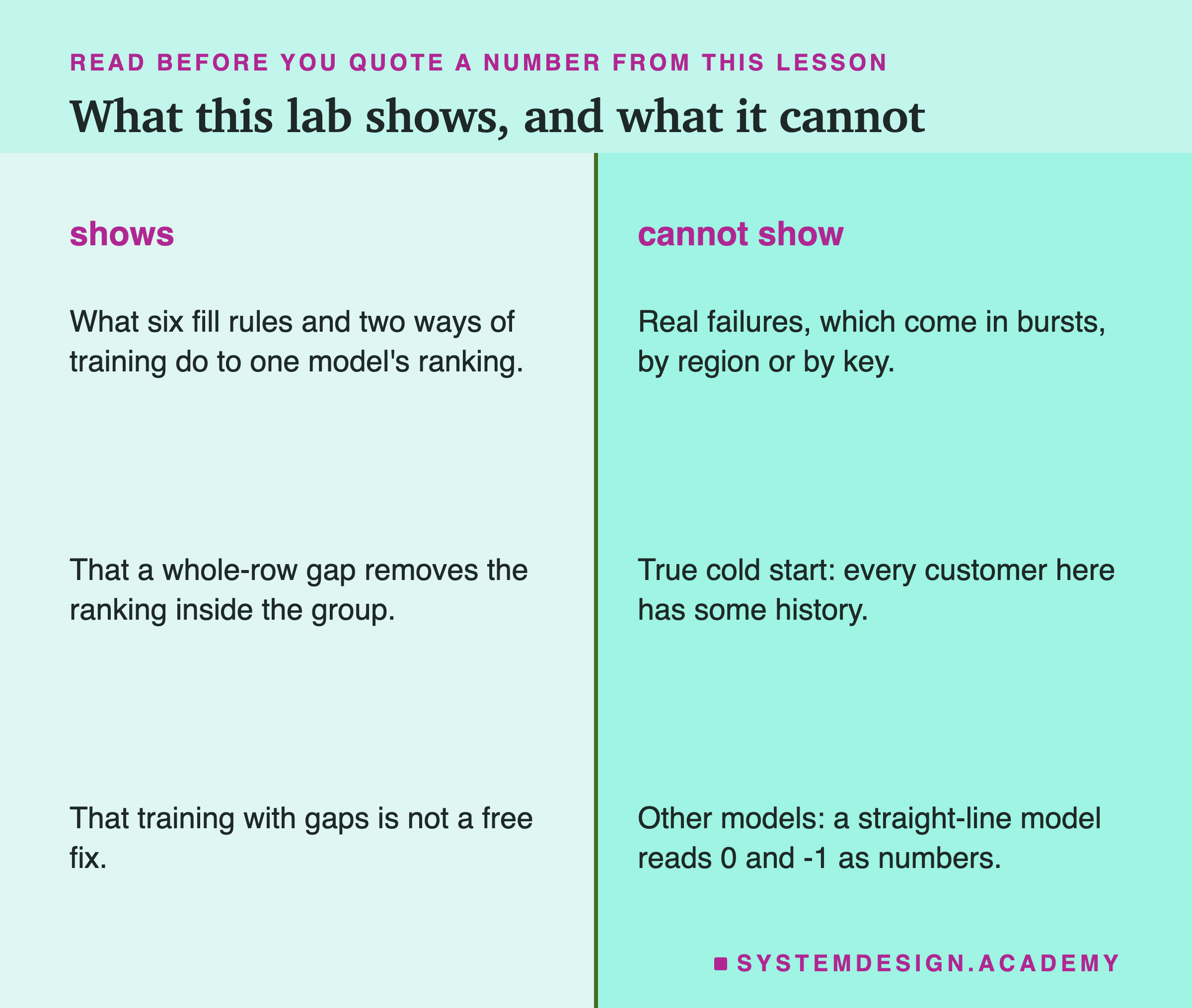
Every gap is simulated, and random. Real failures come in bursts: one region's store slows down, one shard loses its keys, one night's job fails. A random draw spreads failures evenly over customers, which is the kindest case. If failures hit good customers more often, the costs here would be larger.

No true cold start. The "new" customers all had at least one order. A truly brand-new customer would have even less to go on.

Rows fail together. Either all six columns or a fixed four go missing. I never tested one missing column at a time.

The training gap rate equals the serving rate. A real team cannot know the failure rate in advance, and I did not test a mismatch between the two.

One model, one shop, one confound I can name. The training months had a higher buy rate than the test months, 23.4 percent against 19.7 percent overall. Part of what "training with gaps" got wrong comes from that shift, not from gaps as such. Two rules changed after the results, and both are labelled in the lab: the corrected 1 percent intervals and the four post-results questions. And I report no timings, because the machine was shared.

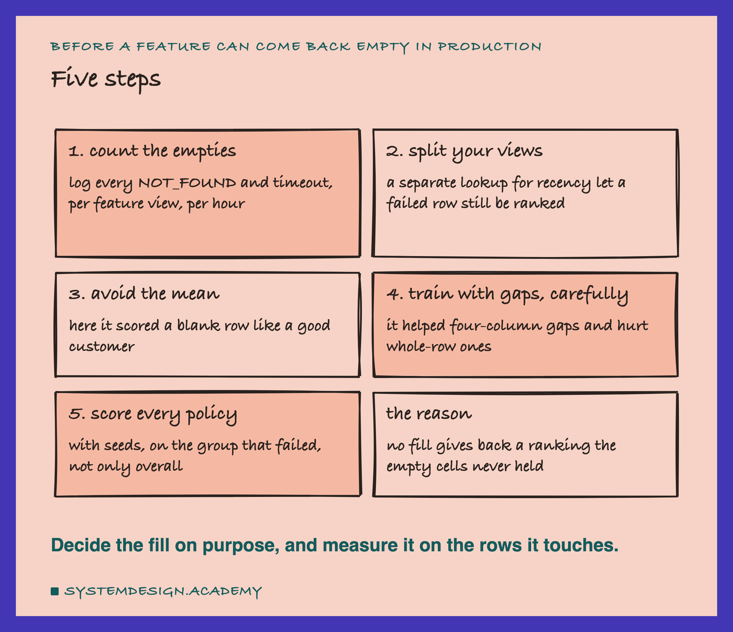
These are the steps I would take the next time a model reads features from a live store.

1. Count the empties. Log every NOT_FOUND and timeout, per feature view, per hour. A fill policy you never see working is a fill policy you never check.

2. Split your feature views where you can, and measure gap training with it. At 20 percent, keeping recency and tenure alone, on the clean model, only moved the loss from 0.0529 to 0.0482. Together with gap training it reached 0.0241.

3. Do not fill counts and money with the mean. Use the median, or leave NaN for a model that handles it.

4. Train with gaps only after measuring. It helped one kind of failure and hurt the other.

5. Score every policy on the rows it touches, with seeds and a paired bootstrap, not only overall.

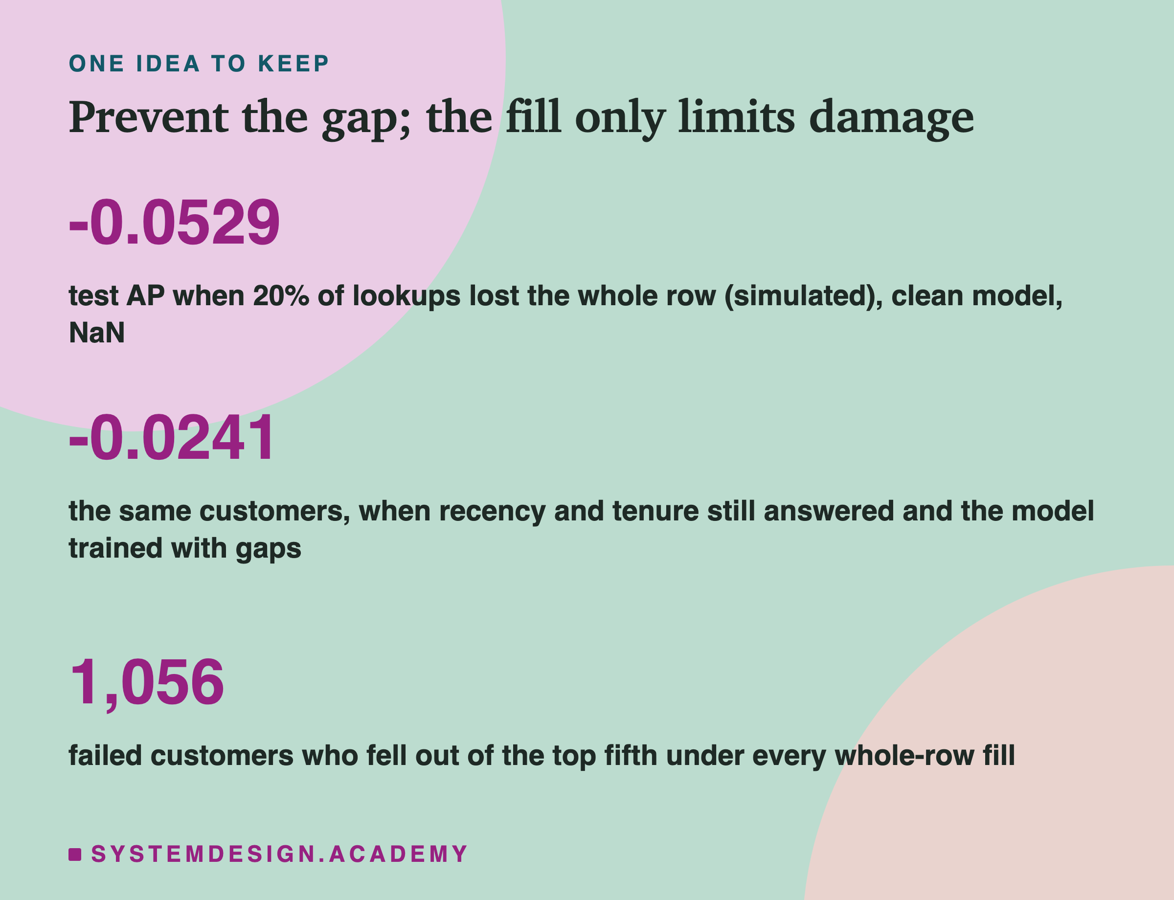
a fill policy decides where the missing customers land, never how they rank against each other. When a whole row is gone, no fill gives it back. Spend your effort on keeping the row, or part of it, available, and then choose the fill on purpose.