Every lesson so far has used qwen2.5:3b, a model with about 3.09 billion weights. A weight is one of the numbers the model learned during training; lesson 4's keys and values, for example, come from multiplying by such numbers. All 3.09 billion of them have to sit in memory for the model to run.

How much memory that takes depends on how precisely each number is stored. Store every weight as a 16-bit number and the model needs about 6 GB. Store them more roughly and it needs less. The model qwen2.5:3b that Ollama downloads by default is already stored roughly, at about 5 bits per weight, which is why it is under 2 GB.

Storing numbers with fewer bits is called quantization. Think of a photo saved at lower quality: the file gets much smaller, and most of the time you cannot see the difference, but look closely at the fine details and some are gone.

This lesson measures exactly that for a language model. It downloads the same model in three forms, and compares their size, their next-word odds, their answers and their speed on my laptop. It turns out that a smaller file does not only save memory; it also makes the model write faster, for a reason that connects back to lesson 3.

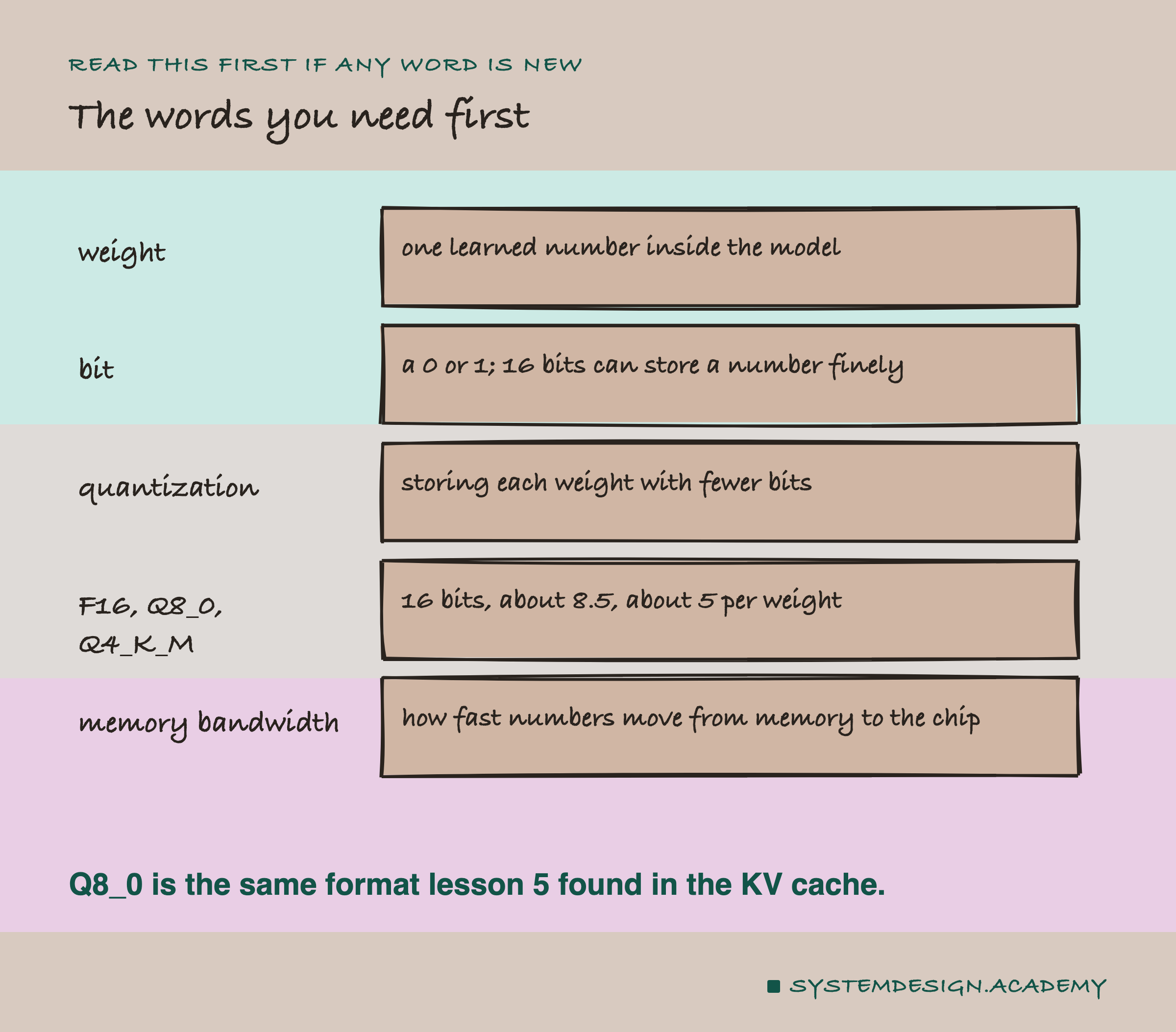
Weight. One of the numbers a model learned during training. qwen2.5:3b has about 3.09 billion of them.

Bit. The smallest unit a computer stores, a 0 or a 1. With 16 bits you can tell apart 65,536 different values; with 8 bits, 256; with 4 bits, only 16.

Quantization. Storing each weight with fewer bits, which means rounding it to the nearest of fewer possible values.

F16, Q8_0, Q4_K_M. The names Ollama and the llama.cpp project use for three formats: 16-bit numbers; 8-bit numbers with a shared scale; and a mix that is mostly 4-bit. You will see these names in model tags.

Memory bandwidth. How many bytes a second can travel from memory to the chip that does the arithmetic. It matters more than you might expect, as the speed slide shows.

The lab used three versions of the same model, all from Ollama's library: qwen2.5:3b (Q4_K_M), qwen2.5:3b-instruct-q8_0 (Q8_0) and qwen2.5:3b-instruct-fp16 (F16). They are the same trained model; only the storage of the weights differs.

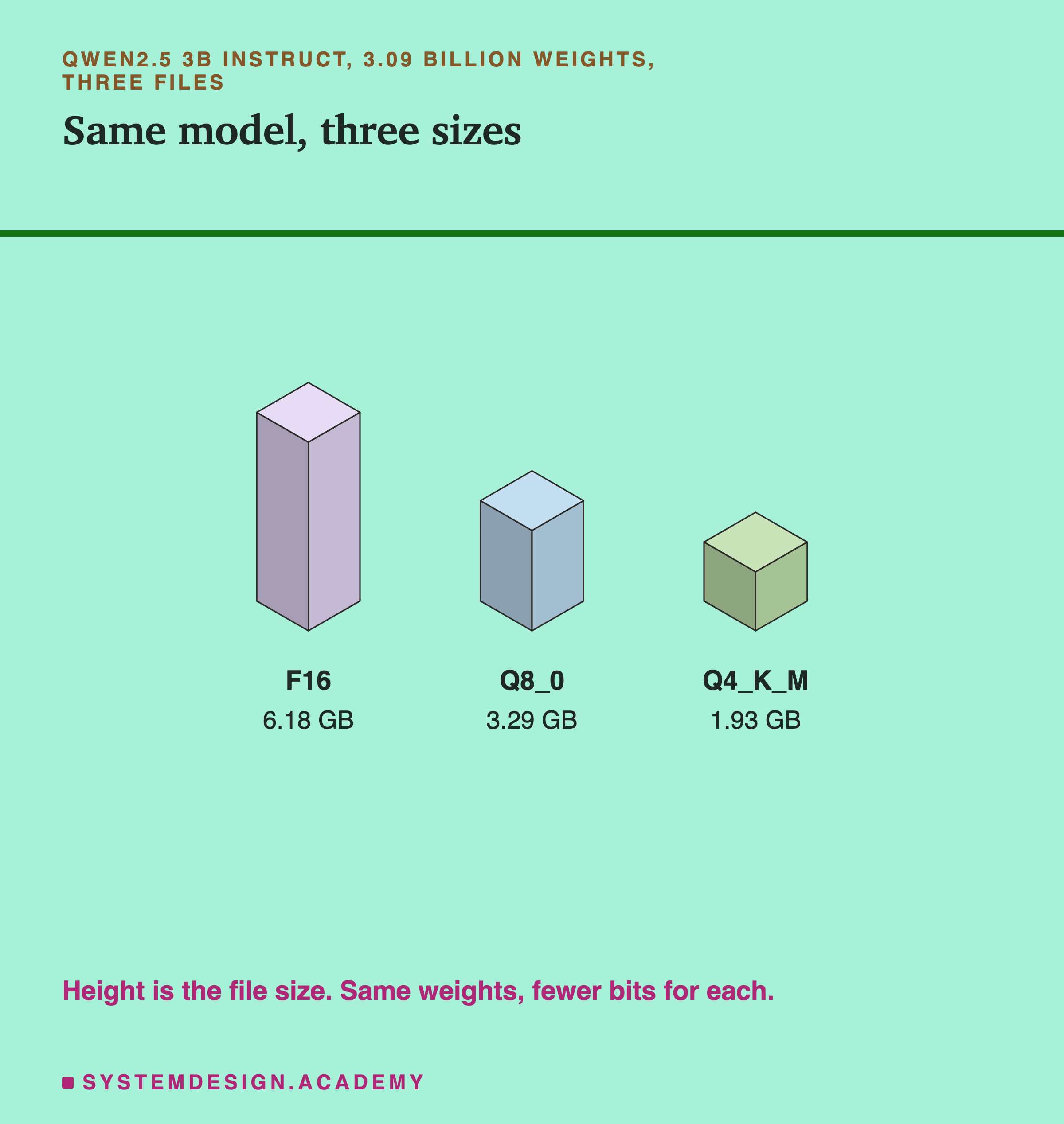
The files were 6.18 GB, 3.29 GB and 1.93 GB. Loaded with a 4,096-token window, Ollama reported 6.34, 3.44 and 2.09 GB, the file plus a little room for the window and working space.

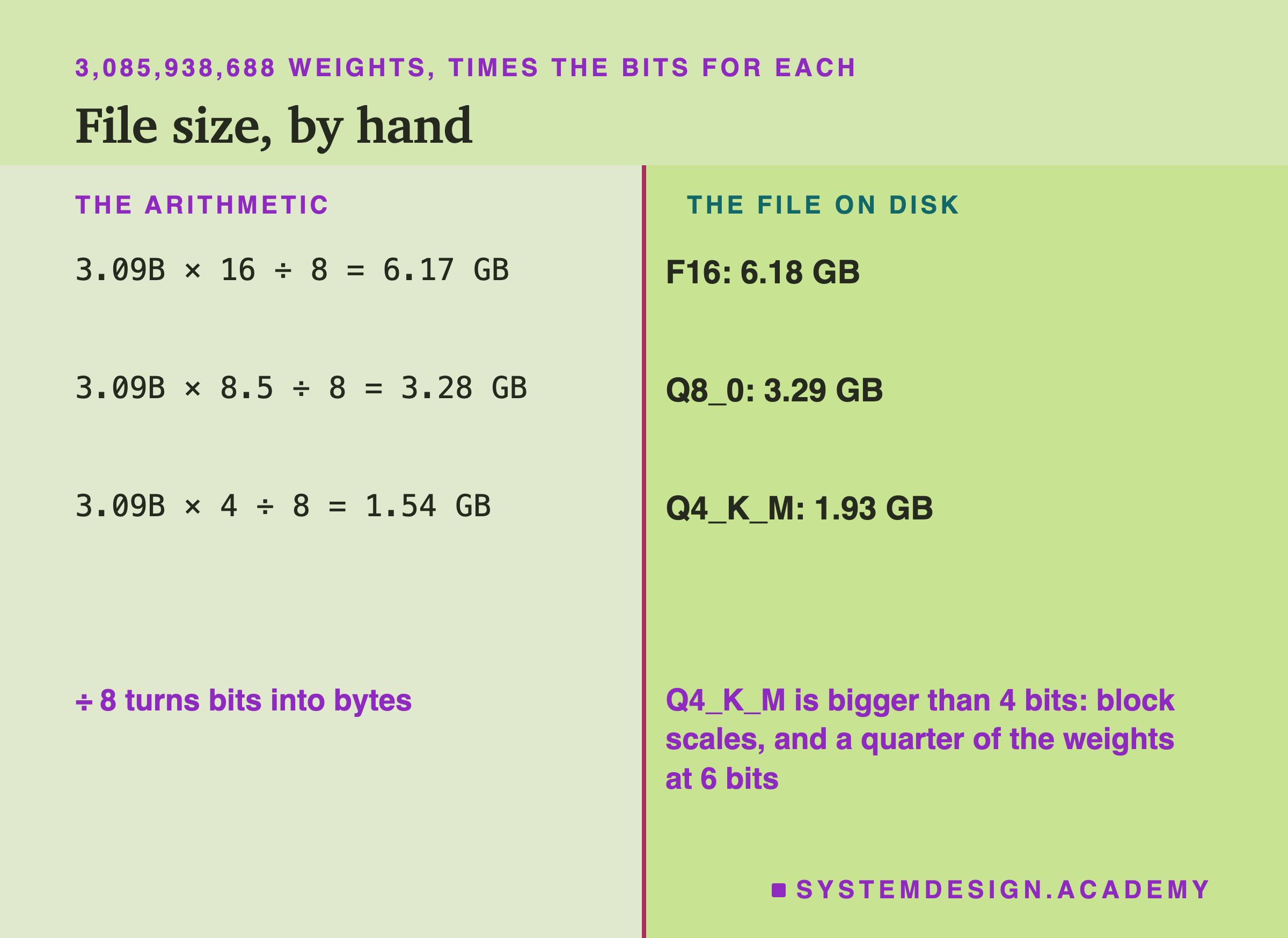
You can work the sizes out by hand. There are 3,085,938,688 weights. At 16 bits each, that is 3.09 billion × 16 ÷ 8 bytes, about 6.17 GB, almost exactly the F16 file. At 8.5 bits, about 3.28 GB, almost exactly the Q8_0 file. At a pure 4 bits it would be 1.54 GB, but the Q4_K_M file is 1.93 GB, for two reasons of about equal size. Each block of 4-bit weights also stores its own scale and minimum, which brings those weights to about 4.5 bits each. And about a quarter of the weights, including the table that turns tokens into numbers, are stored in a 6-bit format. Dividing the file size by the number of weights gives 5.0 bits per weight on average.

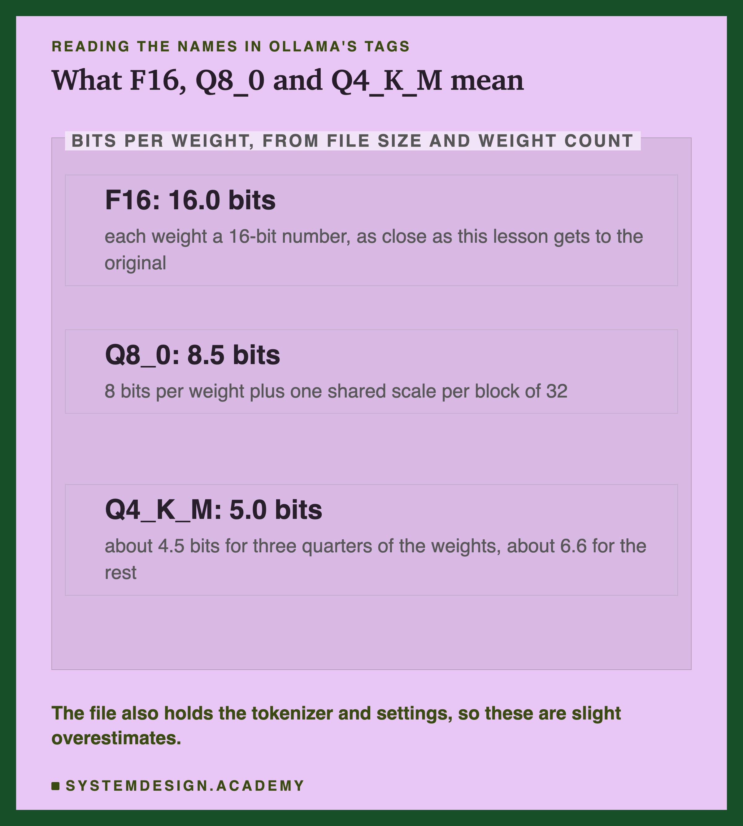
F16 stores each weight as a 16-bit floating-point number, a format that keeps about three significant digits and a wide range of sizes. This lesson treats it as the reference, the version closest to the model as it was trained.

Q8_0 groups the weights into blocks of 32. Each block keeps one shared scale, a 16-bit number, and each weight in the block is stored as an 8-bit whole number from −127 to 127 that is multiplied by the scale. That is 32 bytes for the weights plus 2 for the scale, 34 bytes per 32 weights, which is 8.5 bits per weight. If that sounds familiar, it is the same q8_0 format that lesson 5 found this laptop's Ollama using for the KV cache.

Q4_K_M is a mix from the llama.cpp project, which is the engine Ollama runs. About three quarters of the weights are stored as 4-bit numbers in blocks that carry their own scales, about 4.5 bits each once those are counted. About a quarter, chosen tensor by tensor (a tensor is one table of weights), are stored in a 6-bit format; in this file that includes the token table and the value weights of every layer. The "K" names the family of methods and the "M" means the medium-sized mix. ollama show --verbose lists each tensor's format, and the lab measured the result as 5.0 bits per weight on average.

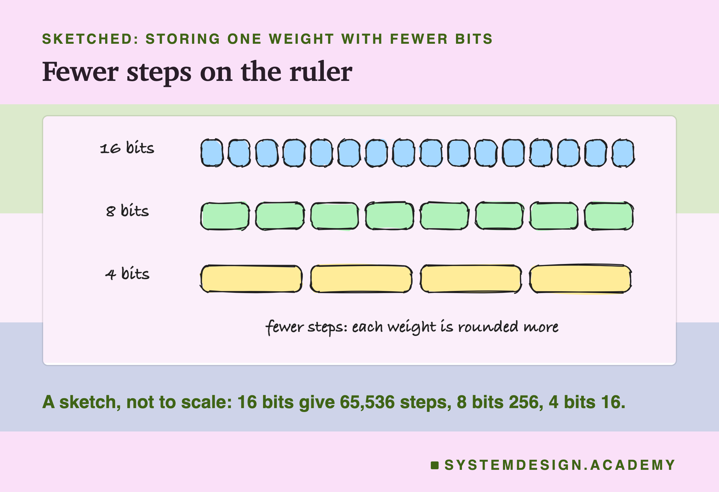
Think of a ruler. A ruler marked in millimetres lets you record a length precisely. A ruler marked only in centimetres forces you to round every length to the nearest centimetre. Quantization swaps a fine ruler for a coarse one.

With 8 bits and a scale shared by 32 weights, the steps are fine: in the playground at the end of this lesson, the largest change to eight sample weights is 0.0032. With 4 bits, there are only 16 steps (the box uses 15, from −7 to 7), and the largest change is 0.0557, about seventeen times as much. In proportion, small weights suffer most: at 4 bits, three of the eight sample weights round to exactly zero.

One rounded weight hardly matters. The question is what billions of slightly rounded weights do together. That is what the next measurements test.

This script asks each of the three files for the next word after "The capital of France is", with its probability, and then times how fast each writes 64 tokens.

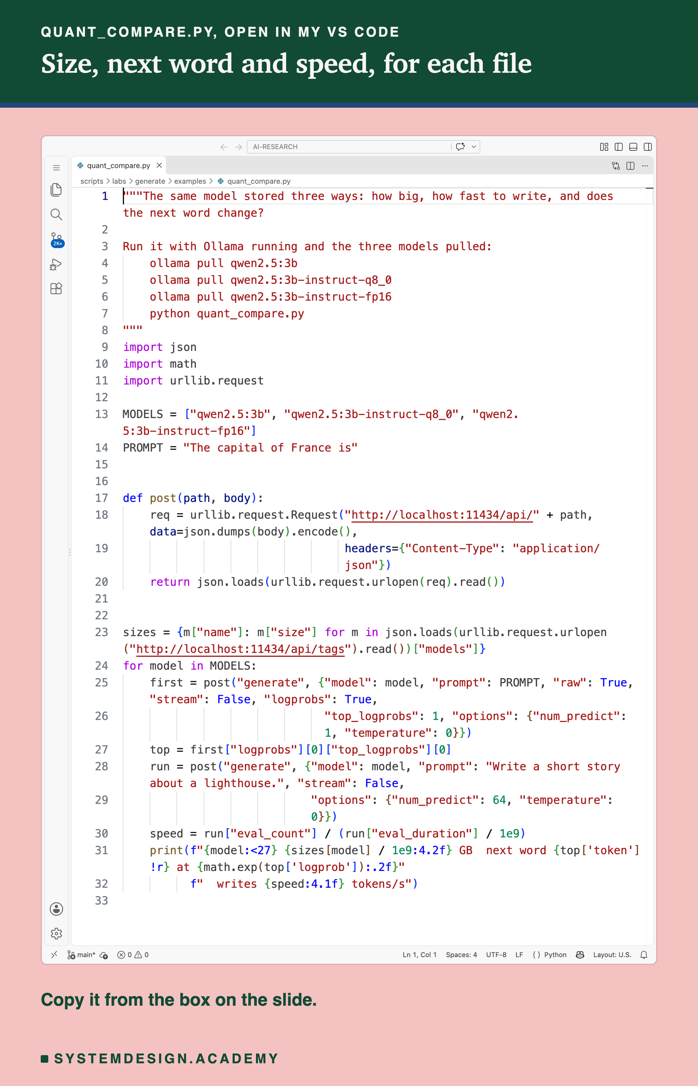
Before you run this lab. It uses qwen2.5:3b, qwen2.5:3b-instruct-q8_0 and qwen2.5:3b-instruct-fp16, running in Ollama on your own computer. If you have not set that up yet, the lab setup guide shows how to install Ollama, download the models and check that everything works, on macOS, Windows or Linux. You can use a different model instead: the guide shows the one line to change, and your numbers will differ from the ones in this lesson.

"""The same model stored three ways: how big, how fast to write, and does the next word change?

Run it with Ollama running and the three models pulled:
    ollama pull qwen2.5:3b
    ollama pull qwen2.5:3b-instruct-q8_0
    ollama pull qwen2.5:3b-instruct-fp16
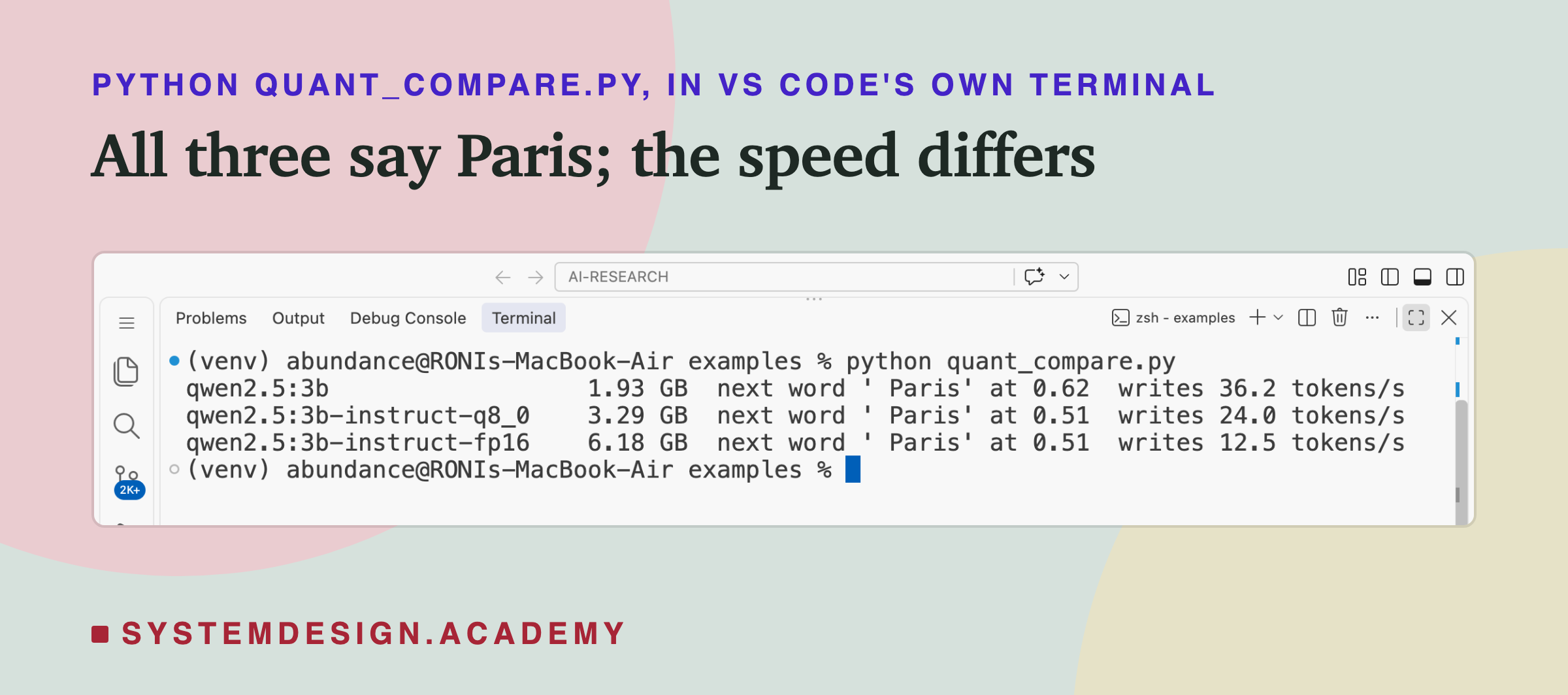
    python quant_compare.py
"""
import json
import math
import urllib.request

MODELS = ["qwen2.5:3b", "qwen2.5:3b-instruct-q8_0", "qwen2.5:3b-instruct-fp16"]
PROMPT = "The capital of France is"


def post(path, body):
    req = urllib.request.Request("http://localhost:11434/api/" + path, data=json.dumps(body).encode(),
                                 headers={"Content-Type": "application/json"})
    return json.loads(urllib.request.urlopen(req).read())


sizes = {m["name"]: m["size"] for m in json.loads(urllib.request.urlopen("http://localhost:11434/api/tags").read())["models"]}
for model in MODELS:
    first = post("generate", {"model": model, "prompt": PROMPT, "raw": True, "stream": False, "logprobs": True,
                              "top_logprobs": 1, "options": {"num_predict": 1, "temperature": 0}})
    top = first["logprobs"][0]["top_logprobs"][0]
    run = post("generate", {"model": model, "prompt": "Write a short story about a lighthouse.", "stream": False,
                            "options": {"num_predict": 64, "temperature": 0}})
    speed = run["eval_count"] / (run["eval_duration"] / 1e9)
    print(f"{model:<27} {sizes[model] / 1e9:4.2f} GB  next word {top['token']!r} at {math.exp(top['logprob']):.2f}"
          f"  writes {speed:4.1f} tokens/s")

The lab asked all three files for their ten most likely next words on lesson 1's 24 prompts: 12 with one clear answer, such as "The capital of France is", and 12 open ones, such as "My favourite food is". F16 is the reference.

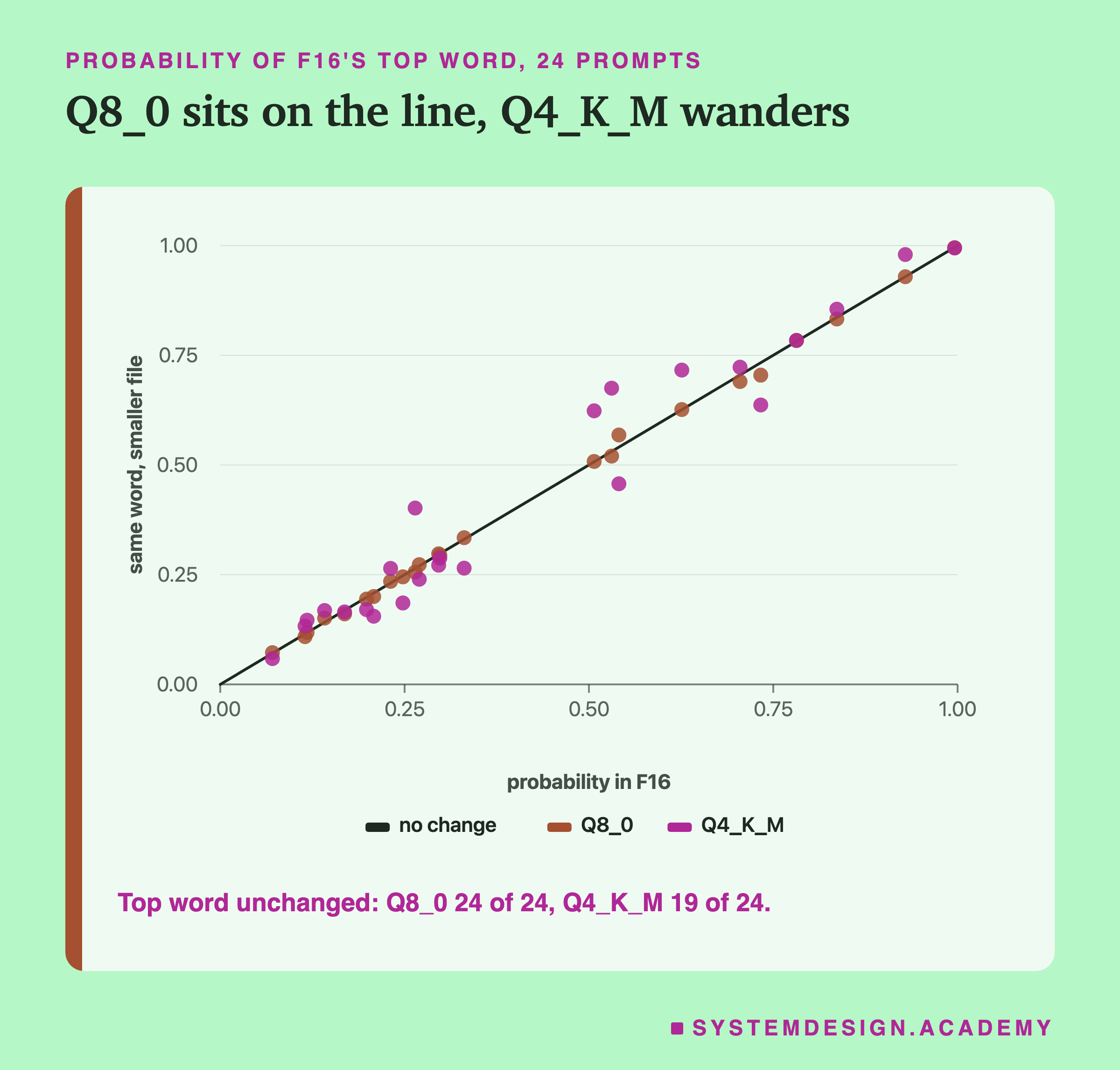
Q8_0 kept F16's top word on all 24 prompts, and the probability of that word moved by a median of 0.4 percentage points, at most 2.8. For practical purposes, it is the same model.

Q4_K_M kept the top word on 19 of the 24. The probability of F16's top word moved by a median of 2.9 points and at most 14.4. That is a visible change, but look at where it happened.

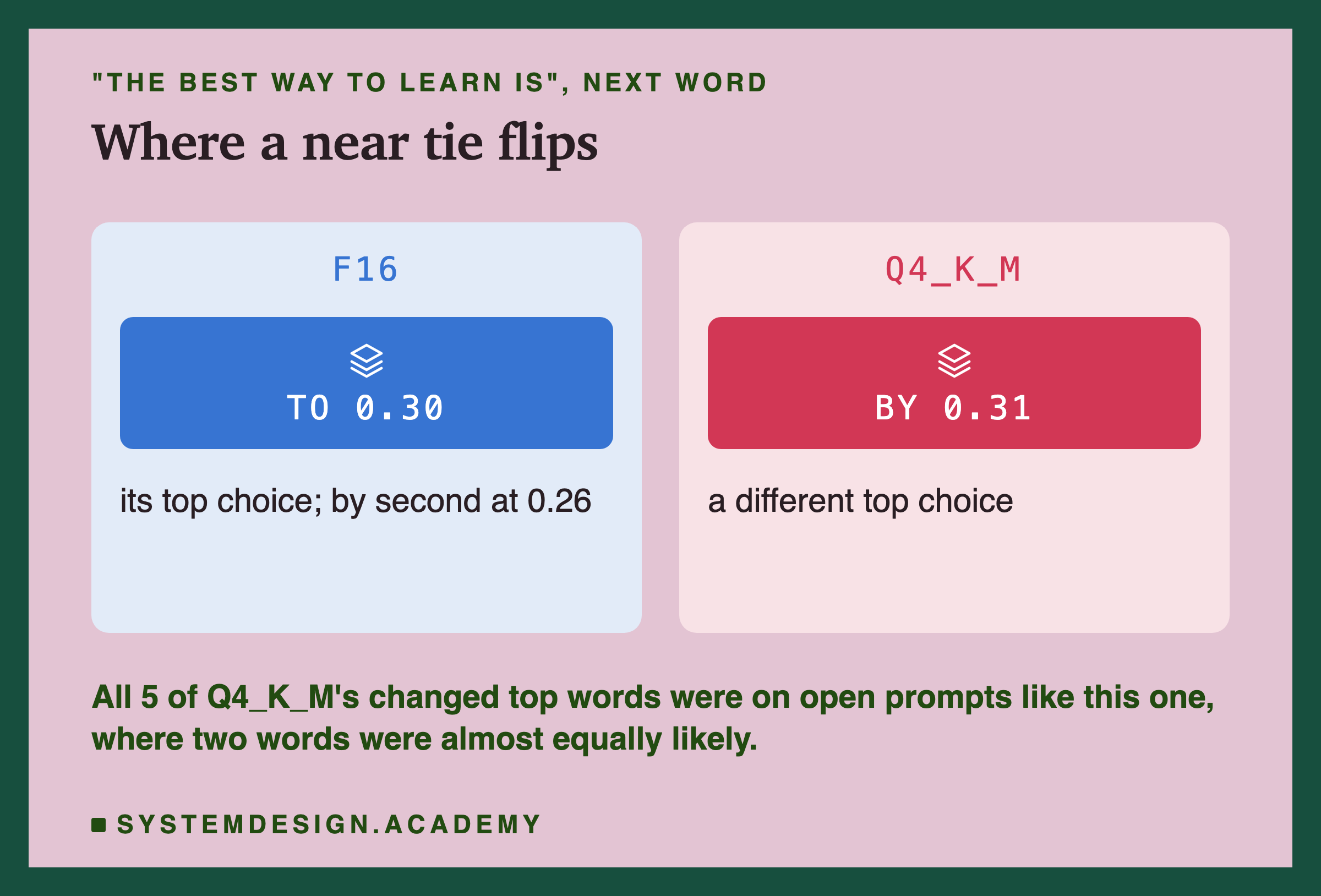
All 5 changed top words were on open prompts, and all 12 prompts with one clear answer kept theirs. After "The best way to learn is", F16 put " to" first at 0.30 and " by" second at 0.26; Q4_K_M swapped them, with " by" first at 0.31. The other four changes were similar: two or more words nearly tied, and a small nudge swapped their order. Where one word was well ahead of the rest, rounding did not change the winner.

Why did rounding leave every clear answer alone and flip only near ties? Lesson 1 showed that the model's odds come from a score for every token in its vocabulary; the scores are turned into probabilities, and the highest score wins. Rounding billions of weights adds a little noise to every score.

When one token's score is far ahead of the rest, as with " Paris" after "The capital of France is", a little noise cannot change the order. The probability may move, and here it did, from 0.51 in the F16 file to 0.62 in the Q4_K_M file, but the winner stays the winner. When two tokens are nearly level, as with " to" at 0.30 and " by" at 0.26 in F16, the same small amount of noise is enough to swap them.

Notice also that the noise does not only make the model less sure. The Q4_K_M file was more sure of " Paris" than the F16 file. Rounding moves scores in both directions; it does not simply make a model "dumber". What it does, on average, is make the smaller file's odds a little different from the original's, and those differences show wherever the original was nearly undecided.

That gives a rule of thumb you can use: quantization is least likely to matter for questions with one clear answer, and most likely to show on open-ended writing, where many continuations are nearly equally likely anyway. The measurement of longer texts on the next slide shows the same thing from another angle.

Odds are one thing; answers are what users see. The lab asked each file 40 two-digit multiplications, such as "What is 47 x 83? Answer with the number only.", through the chat template at temperature 0.

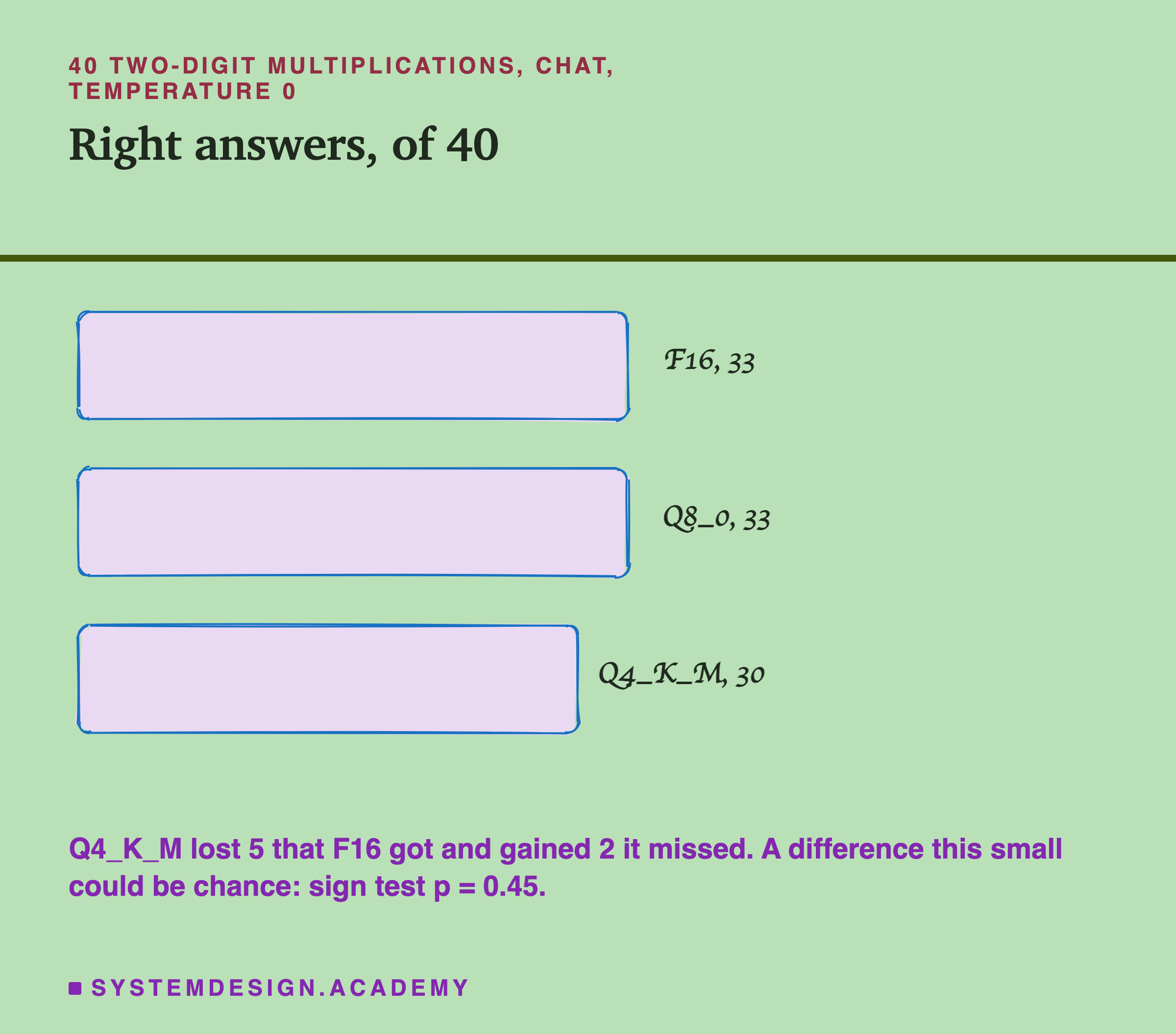
F16 got 33 right and Q8_0 got 33 right, the very same 33. Q4_K_M got 30. That looks like a loss, but look at the details: Q4_K_M got 5 wrong that F16 got right, and 2 right that F16 got wrong. A sign test, which asks how likely a split of 5 against 2 is if neither version is really better, gives p = 0.45, where p is the chance of a split at least this lopsided happening by luck alone. A split like that happens often by chance. With only 40 questions, this lab cannot tell whether Q4_K_M is worse at sums.

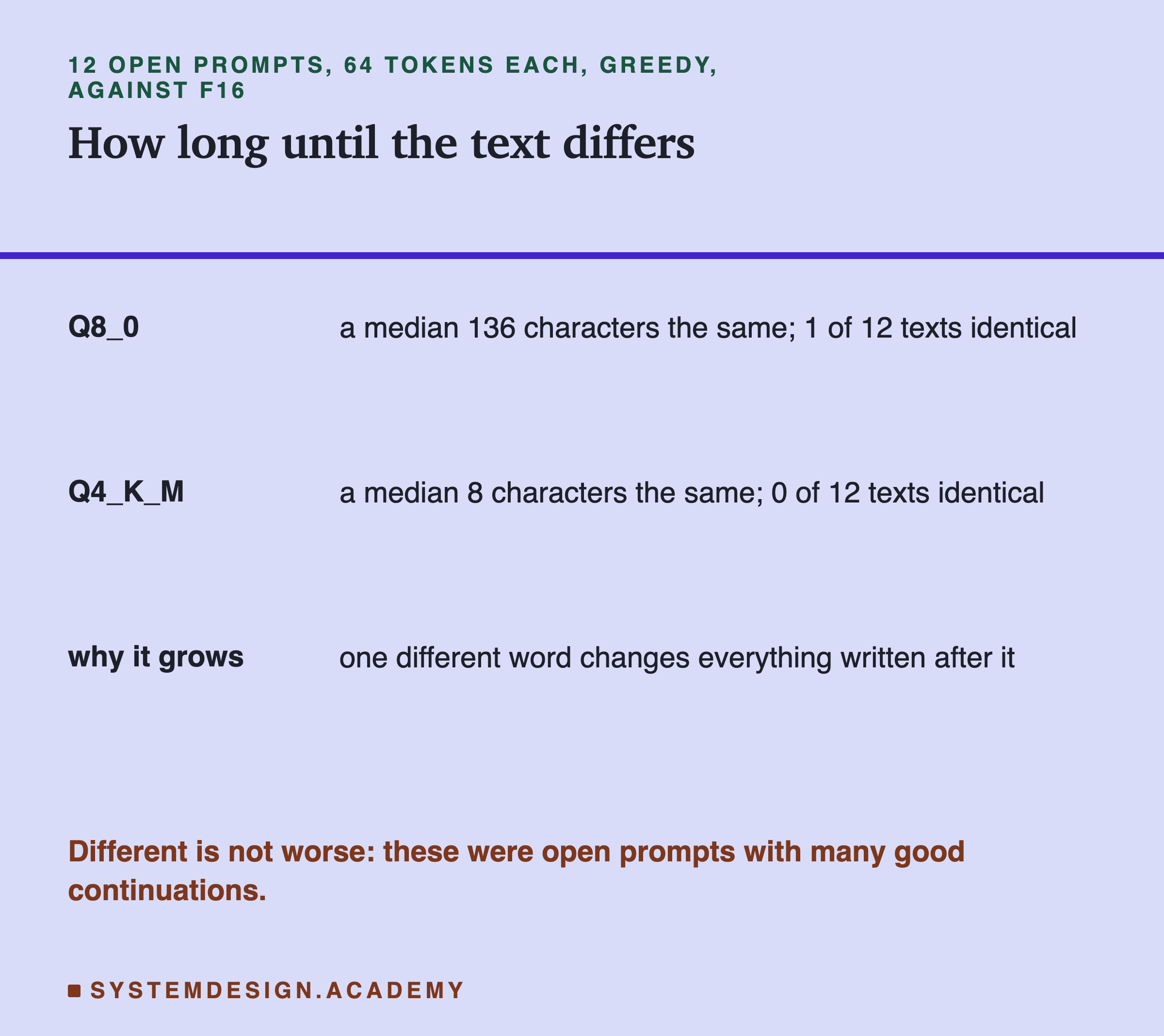
Longer texts show the rounding more. The lab wrote 64 tokens greedily from each of the 12 open prompts and compared each text with F16's. Q8_0's texts stayed the same as F16's for a median of 136 characters before the first difference, and 1 of the 12 was identical all the way. Q4_K_M's texts differed after a median of only 8 characters. That is lesson 2's point again: once one word differs, every later word is written after a different history, so small changes grow. On open prompts, a different text is not a worse text; it is just a different one of many good continuations.

The lab timed each file writing 128 tokens after a prompt of about 1,000 tokens, in 3 rounds with the three files in a shuffled order each round, 6 calls per file.

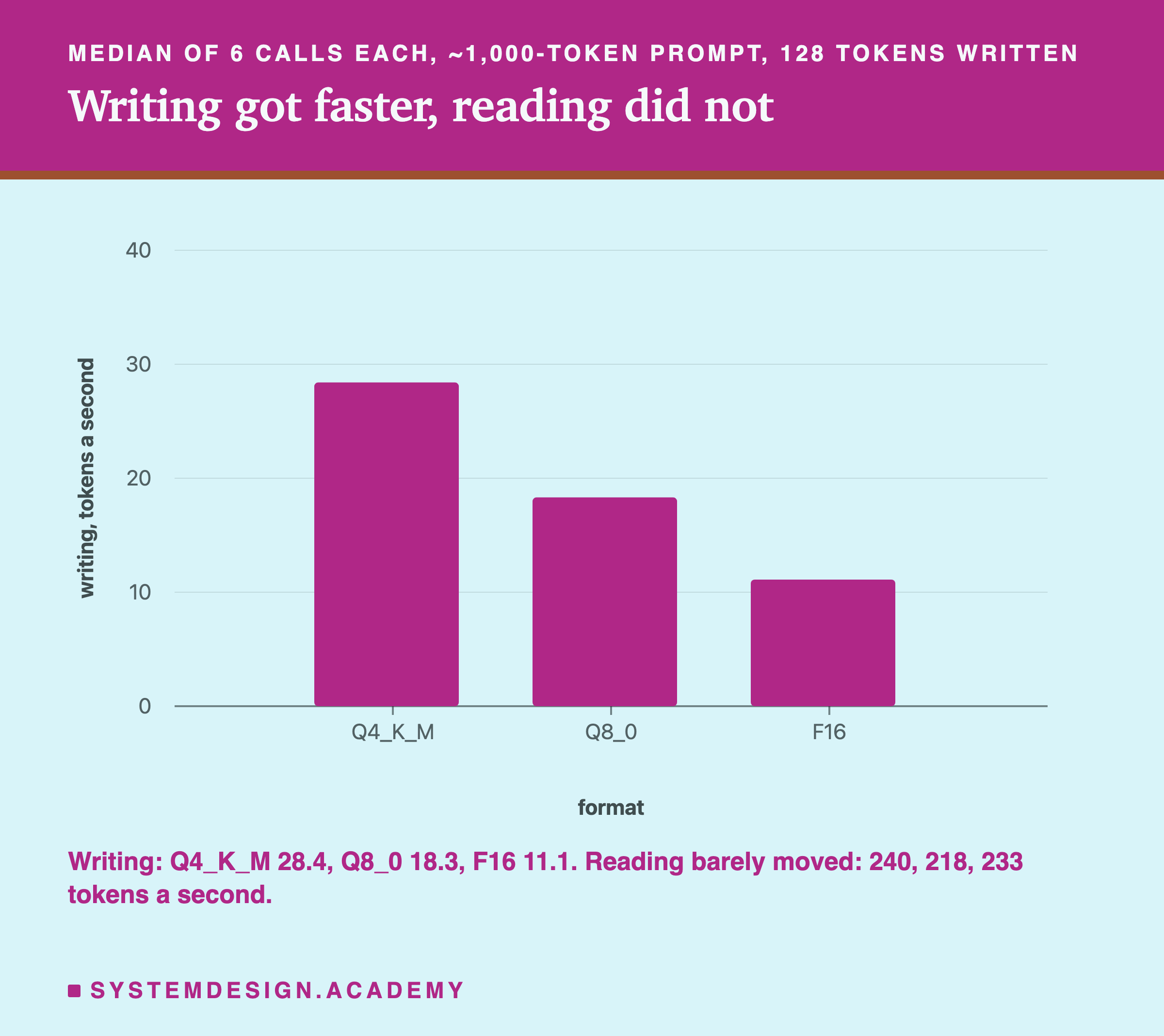
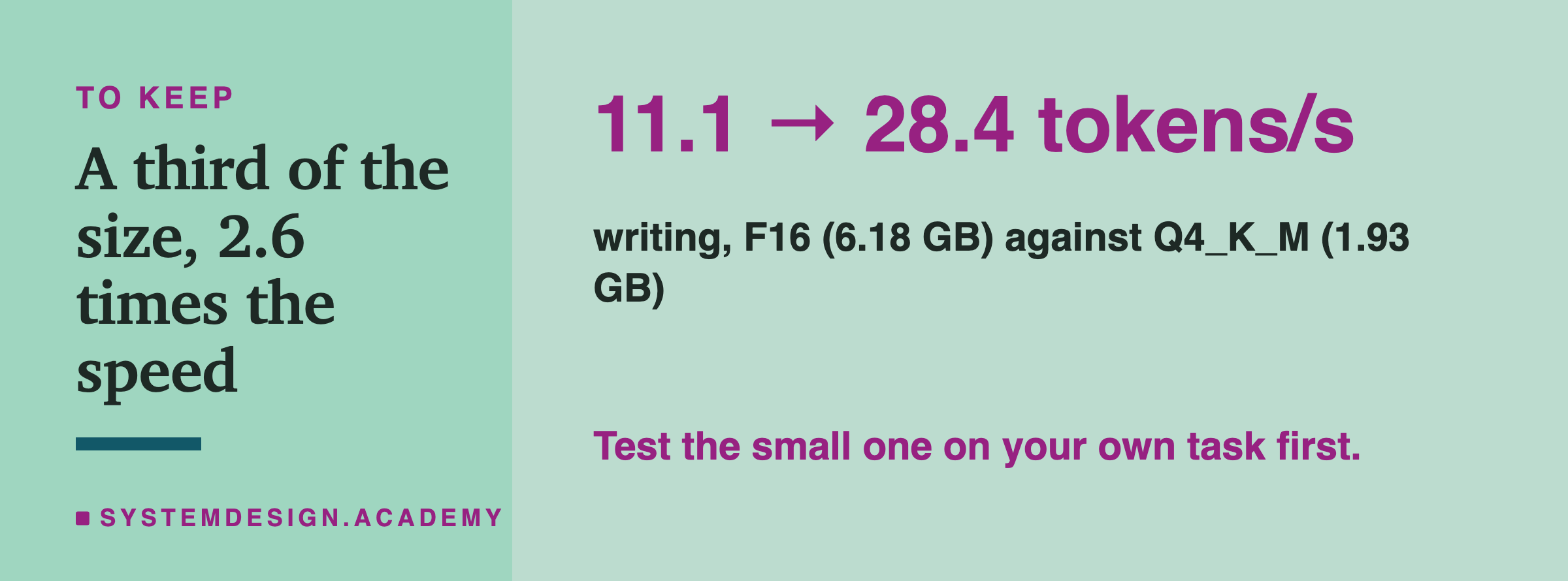
Writing speed rose as the file shrank: 11.1 tokens a second for F16, 18.3 for Q8_0 and 28.4 for Q4_K_M. The smallest file wrote about 2.6 times as fast as the largest. Reading speed hardly moved: 233, 218 and 240 tokens a second, within the laptop's usual noise.

Why would writing depend on the file size? Lesson 3 showed that writing is done one token at a time. For every single token, the chip must use every weight in the model once, and the weights live in memory, so for every token they must be fetched from memory to the chip.

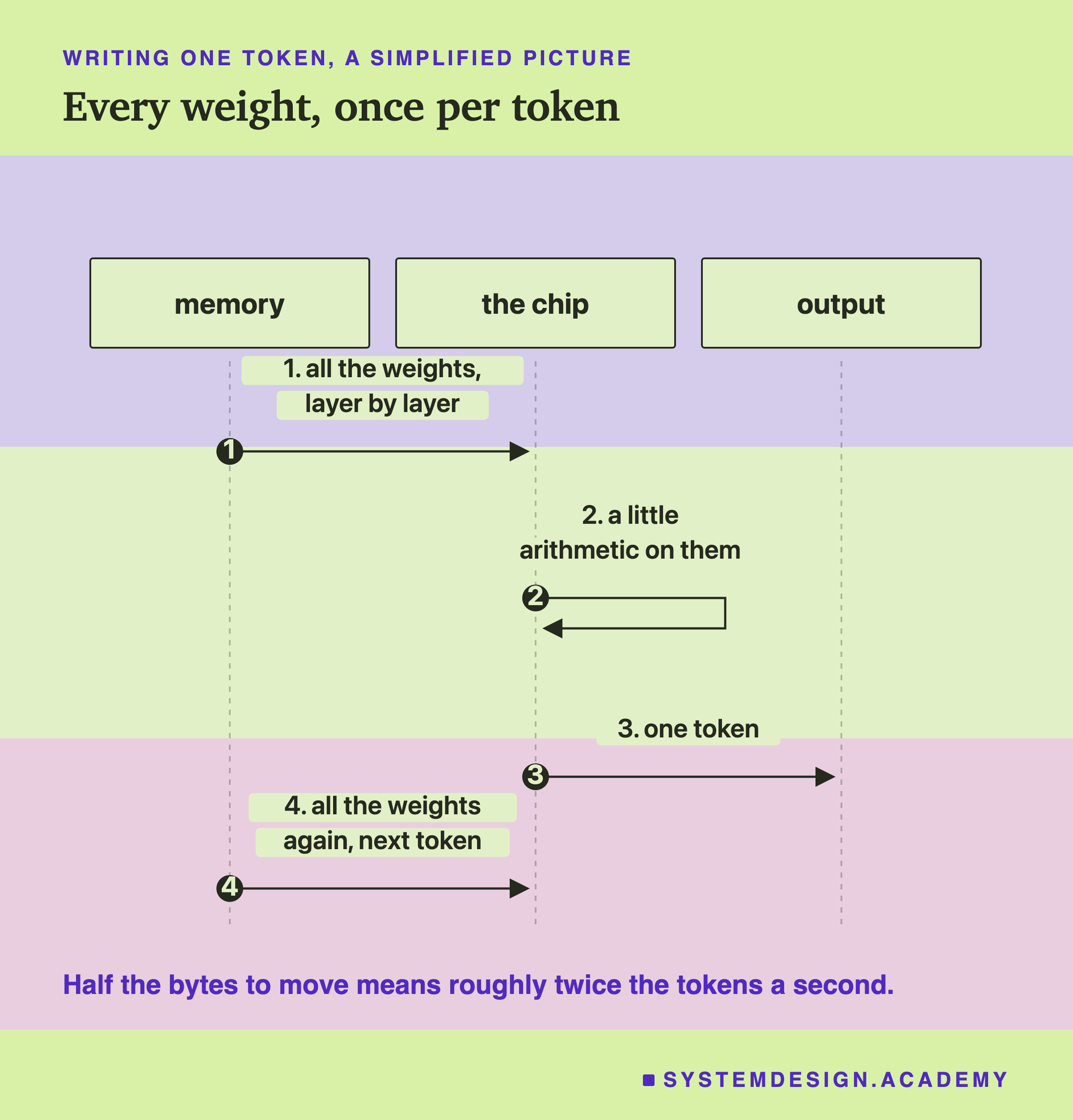
If moving the weights is the slow part, then writing speed times file size should come out roughly the same for all three files: the number of bytes the laptop can move per second.

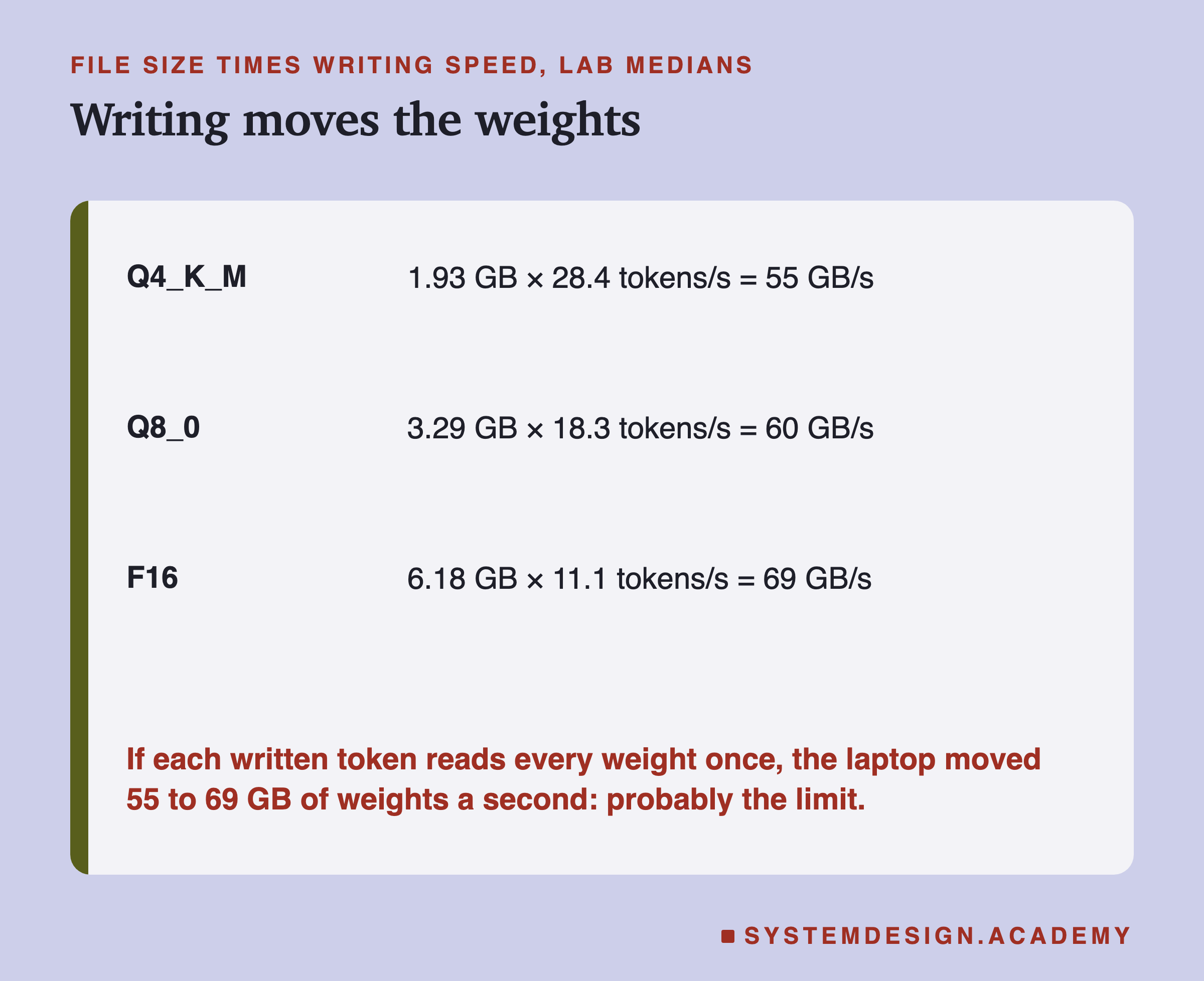
It does, roughly: 1.93 × 28.4 ≈ 55 GB a second, 3.29 × 18.3 ≈ 60, and 6.18 × 11.1 ≈ 69. The figures are not identical, because unpacking 4-bit numbers takes a little arithmetic too, but they are close enough to suggest where the time goes: writing is probably mostly waiting for memory. The gap between them may partly be the extra arithmetic of unpacking 4-bit numbers. This is a calculation from the lab's numbers, not a direct measurement of bandwidth.

Reading a prompt is different. Lesson 3 explained that reading handles many tokens at once, so each weight fetched from memory is used for many tokens before the next is needed, and fetching is no longer the slow part. That is a likely reason reading speed barely changed; the lab measured the speeds, not the cause.

Speed is a welcome surprise, but the main reason people quantize is memory. A model only runs if all its weights fit in memory, alongside the KV cache from lesson 5 and everything else the computer is doing.

Worked by hand with this lesson's bits per weight: a model with 7 billion weights needs about 7 × 16 ÷ 8 = 14 GB at F16, but about 7 × 5 ÷ 8 ≈ 4.4 GB at Q4_K_M's 5 bits. On a laptop with 16 GB, the first barely fits, if at all, once the operating system and a browser are running; the second leaves plenty of room. A model with 70 billion weights needs about 140 GB at F16, about 74 GB at Q8_0's 8.5 bits, and about 44 GB at 5 bits. None of those fits this 24 GB laptop, and only the smallest fits a machine with 64 GB.

So quantization often decides which model you can run at all, not just how fast it runs. A bigger model at 5 bits can be a better choice than a smaller model at 16 bits, if both fit. This lab did not compare models of different sizes, so it cannot say where that line falls for your task.

Remember the other costs from earlier lessons too. The window you set reserves KV cache memory on top of the weights, and on this laptop that cache was itself stored in q8_0, which is quantization applied to the keys and values instead of the weights.

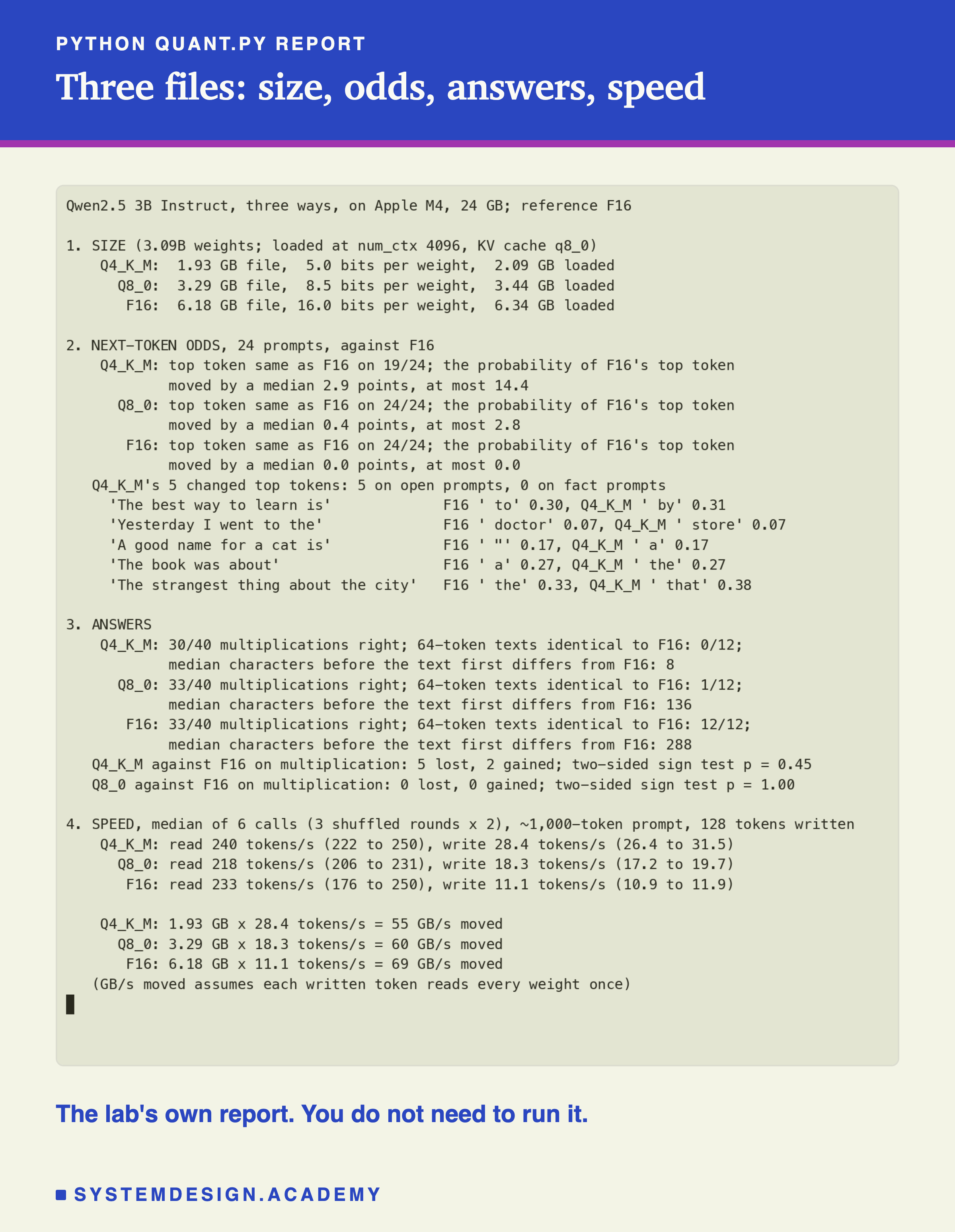
The lab is scripts/labs/generate/quant.py. It reads the sizes from Ollama, loads each file with the same window, and runs the four measurements. The speed test uses a unique first line in every prompt, lesson 6's guard against reuse, and checks that no prompt was read impossibly fast.

Two details in the report were added after reading the first version. The first listed only "19 of 24" for Q4_K_M, which sounds like a model that gets a fifth of its words wrong; listing the five changes showed they were all near ties on open prompts. The second compared 30 against 33 right answers; the sign test shows that difference is too small to call.

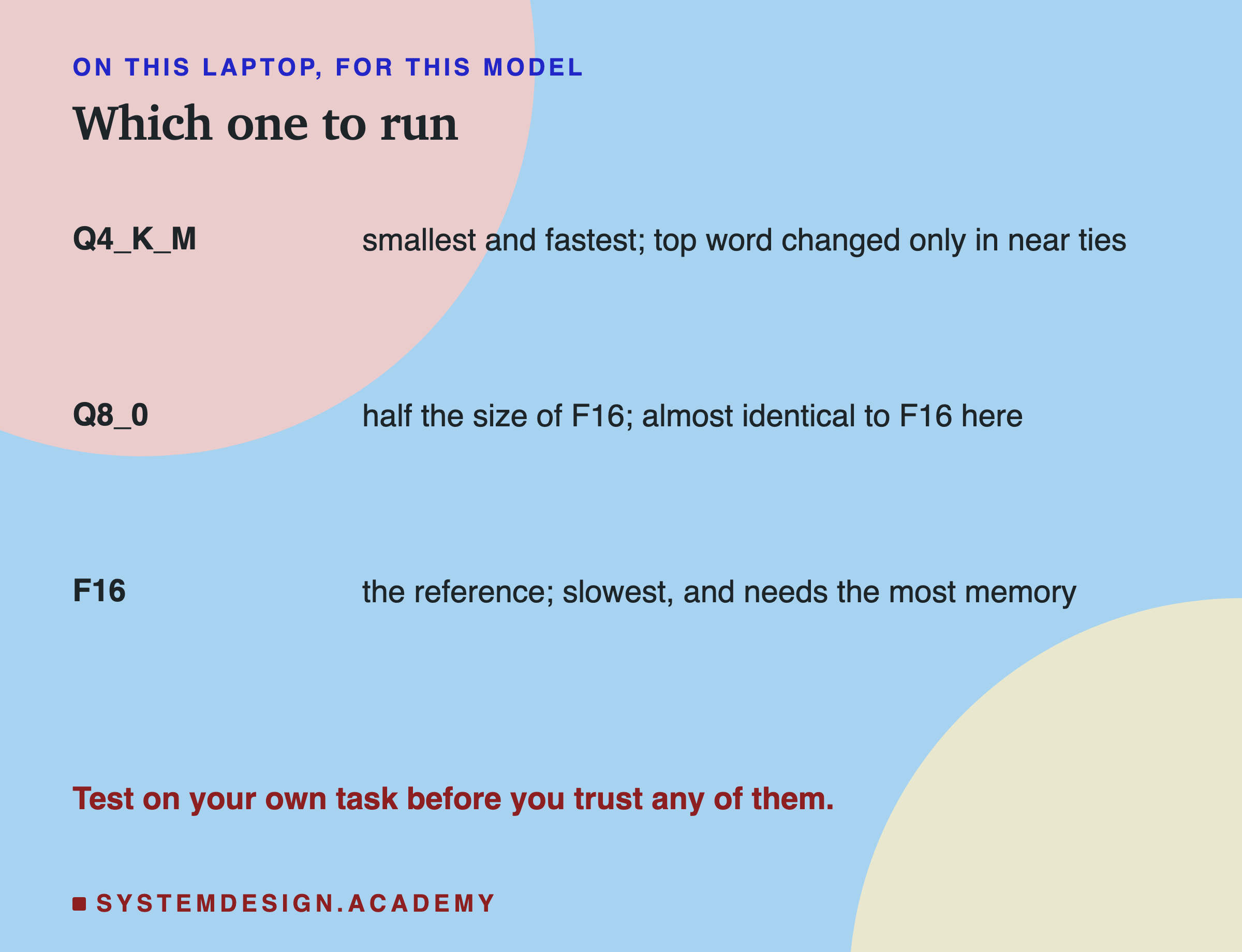
On this laptop, for this model and these tests, the choice looks like this. Q4_K_M is a third of the size of F16 and writes about 2.6 times as fast; on these tests its differences were small and mostly on near ties. Q8_0 is about half the size of F16, writes about 1.6 times as fast, and was almost indistinguishable from F16. F16 is the reference and the slowest.

This is probably why many of Ollama's default tags are a 4-bit mix: it is a good trade for most people on most machines. But "these tests" is doing a lot of work in that sentence. This lab used short prompts and simple sums. A task that depends on fine detail, such as exact code, careful arithmetic in long chains or a language the model saw little of, may suffer more from rounding. The only fair test is your own.

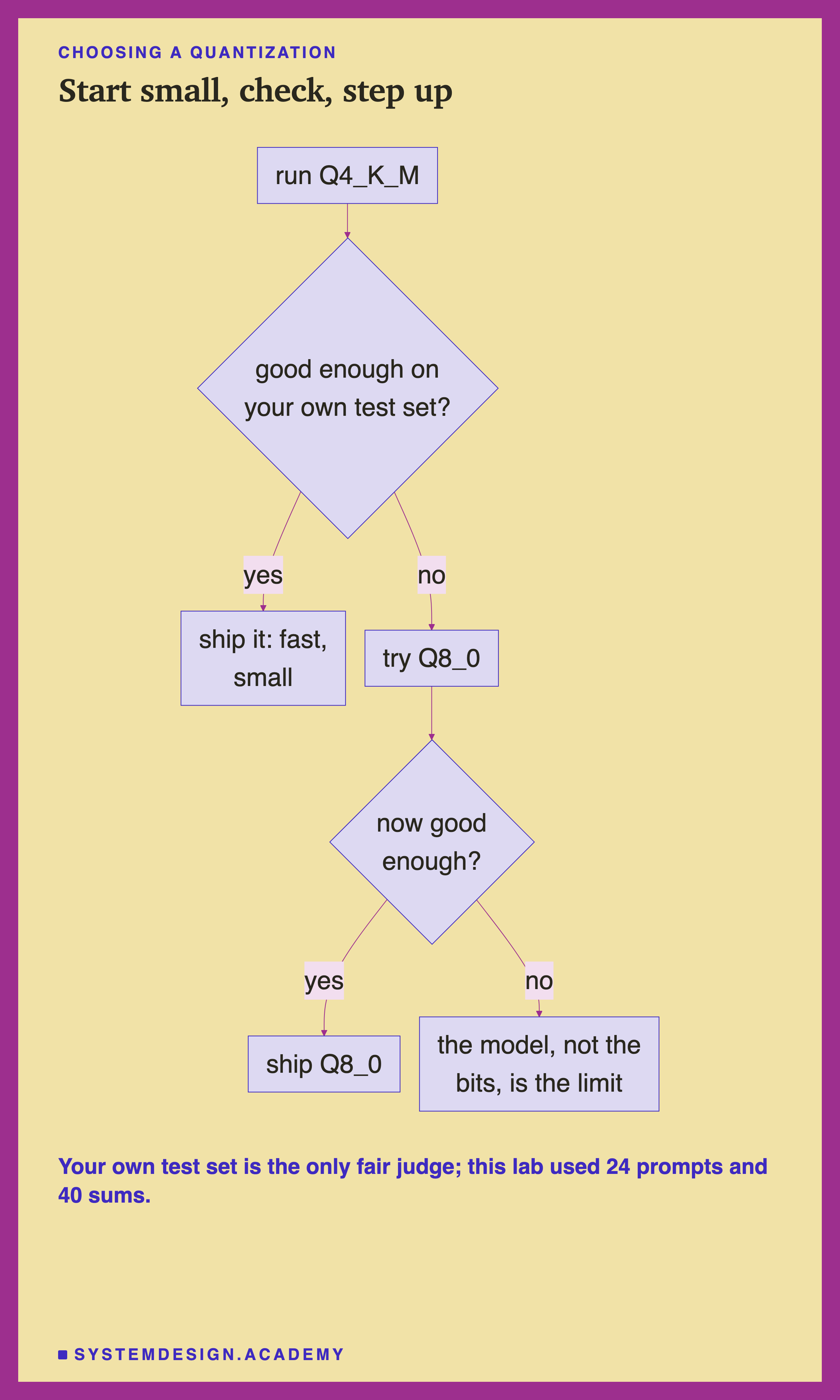
A sensible order is to start with the small file, check it on 20 to 50 examples from your real task, and step up to Q8_0 only if it falls short. If Q8_0 also falls short, the problem is probably the model itself, not how its weights are stored, and a bigger or different model is the answer.

This box has no model. It rounds eight made-up weights to 8 bits and to 4 bits, using one shared scale as Q8_0 does, and then works out the file sizes by hand.

It prints the 8-bit weights, whose largest change is 0.0032, and the 4-bit ones, whose largest change is 0.0557 and where 0.0213, −0.0062 and 0.0555 all became 0.0. Then it prints 6.18, 3.28 and 1.93 GB, close to the three files. Change the weights, or try 6 bits, and watch how the rounding grows. Real formats are cleverer than this box: Q4_K_M gives each group of 32 weights its own scale and minimum, so a group of small weights gets finer steps, and it stores about a quarter of the weights at 6 bits.

The three names. MODELS lists the three Ollama tags. They must be pulled first; the first one is the default qwen2.5:3b, which is the Q4_K_M file.

The file size. /api/tags lists every model Ollama has, with its size in bytes, so the script reads the size rather than guessing it.

The next word. A raw call with "logprobs": True and "top_logprobs": 1 returns the most likely next token and its log probability. math.exp turns the log probability back into an ordinary probability, as in lesson 1.

The speed. A second call writes 64 tokens. eval_count divided by eval_duration, turned from nanoseconds into seconds, gives tokens written per second, the same measure as lessons 3 and 5.

The lab. quant.py does all of this more carefully: 24 prompts instead of one, 40 sums, 12 longer texts, and speed timed in shuffled rounds with medians.

Assuming the default is full precision. qwen2.5:3b is already a Q4_K_M file at about 5 bits per weight. Check with ollama show.

Calling a small difference a loss. 30 against 33 right answers had a sign test p of 0.45: too close to call with 40 questions.

Testing on one prompt. One prompt showed the same answer, Paris, in all three files. The texts of 64 tokens showed how different they can become.

Forgetting the speed gain. Smaller files write faster on a laptop, most likely because writing is mostly waiting for memory.

Trusting general benchmarks for your task. The trade depends on the task; test on yours.

Comparing speeds from single runs. One run, on a different and shorter prompt, gave 36.2 tokens a second for Q4_K_M; the lab's median was 28.4. Use medians over several runs.

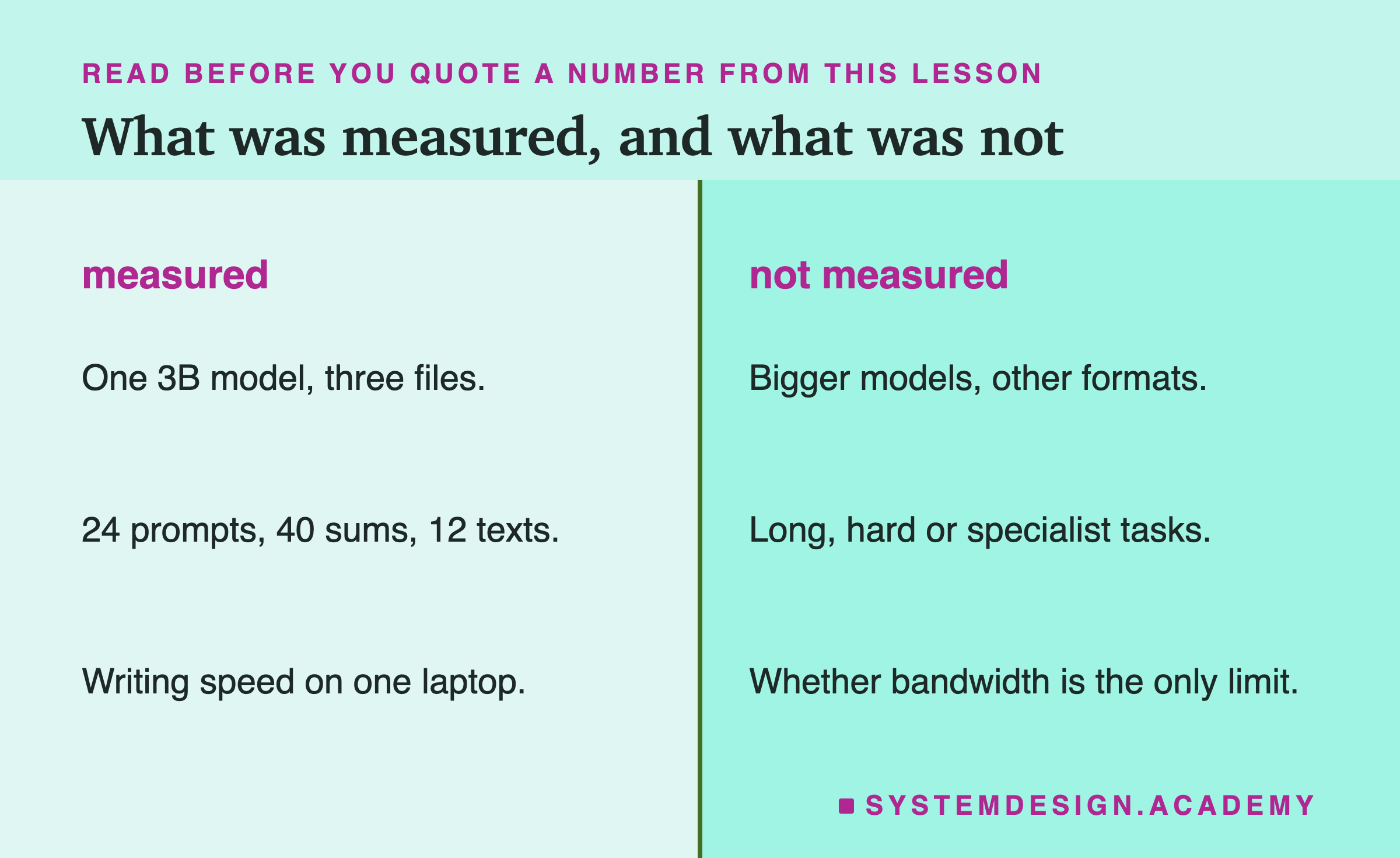
The lab compared three files of one small model on one laptop, with 24 prompts, 40 sums and 12 texts. Larger models are often said to tolerate rounding better and smaller ones worse, but this lab did not test that. It did not test other formats, such as 2-bit or 6-bit files, or tasks that need long exact reasoning. And the bandwidth arithmetic is a calculation from measured speeds and sizes, not a measurement of the memory system itself.

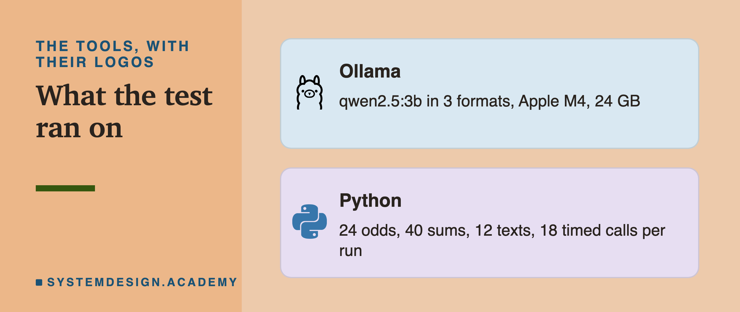
Everything ran locally with Ollama and Python, so you can repeat it on your own machine, if it has room for the 6 GB file.

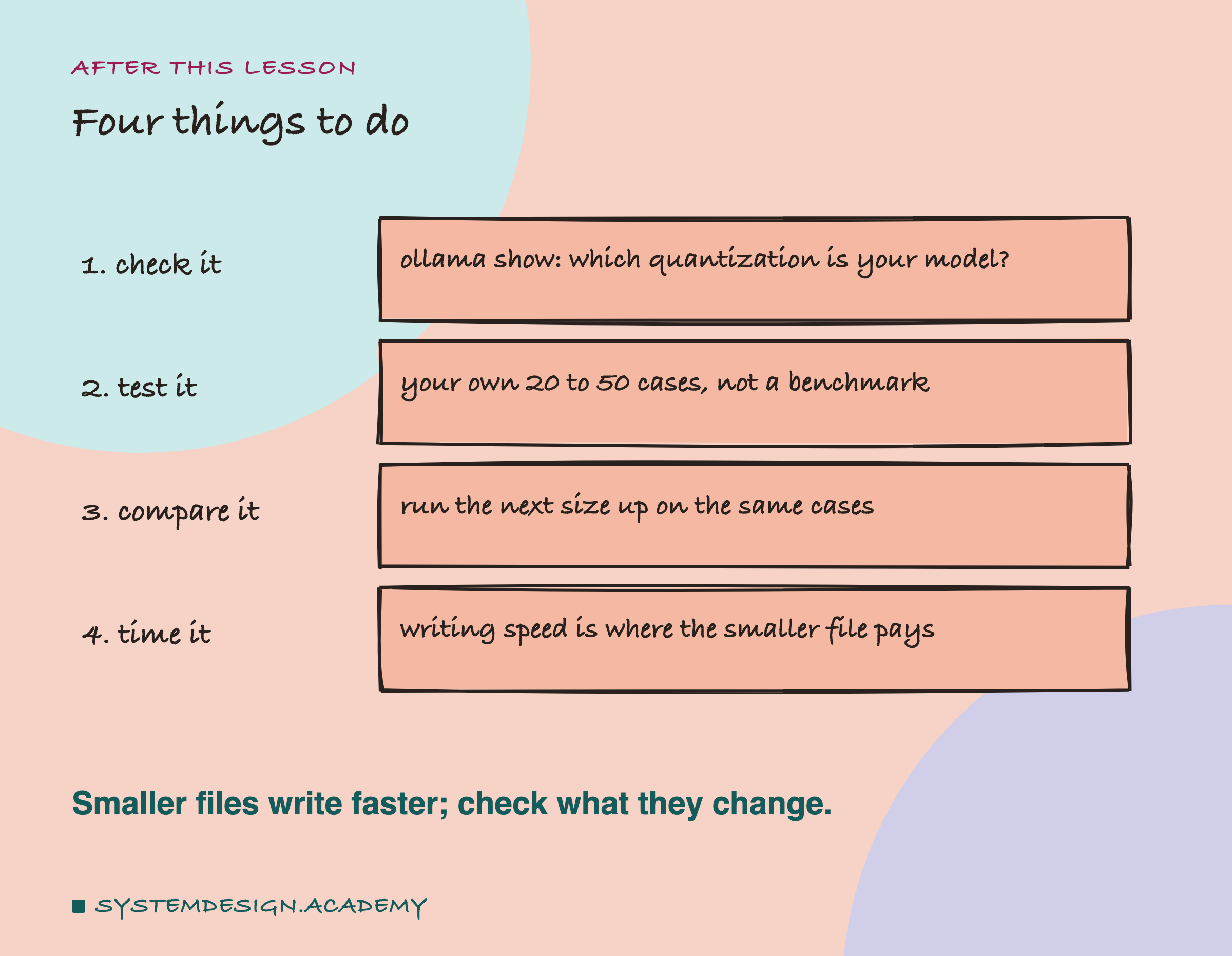
Run ollama show on the model you use and read its quantization line, so you know what you are running. Then collect 20 to 50 real examples from your task, with the answers you expect, and run them through your current file and the next size up. If the scores are the same, keep the smaller file and enjoy the speed. If they differ, look at the examples that changed before deciding: they tell you whether the smaller file fails on something that matters to you.