Imagine a small bakery that opened in a quiet part of town. In its first year the owner kept a careful notebook: for every hour of every day, how many loaves were sold. By the end of the year she knows her shop well. Monday mornings are slow. Saturday mid-morning is the rush. Rainy days are quiet. She uses the notebook to decide how much dough to make each morning, and it works.

Then, in her second year, a new office building opens across the road. Hundreds of new people walk past every morning. The notebook still says what a Monday in March looked like last year, and the owner still bakes for last year's Monday in March. By half past eight the shelves are empty. The notebook was not wrong about last year. It was only about last year, and she was using it for this one.

Nothing in the notebook tells her that the world outside has changed. She finds out from the empty shelves. The fix is simple to say: keep writing in the notebook, and plan from the newest pages, not only the oldest ones. It is harder to do well. How often should she look again? Should she throw away last year's pages, or keep them? And what about the very first morning after the office opened, when there were no new pages yet?

This lesson asks those questions of a computer program that guesses how many bikes a city rents in an hour. I taught it one year, then asked it about every hour of the next year, and I tried three ways of keeping it up to date. The program that was never updated missed by about twice as much as the one updated every month, and most of its error came from guessing too low: it was under the real count in 86% of the hours.

The lesson before this one, the score that lied, was about the test. It showed that picking test hours at random let the program see the rest of each test month while it learned, and that a fair test must keep time in order: learn from the past, then be tested on what came after. That fair test is called a forward split: train on the earlier hours, test on the hours after them. With it, the program's average miss grew from 26.09 bikes an hour to 44.07. Lesson 1 then measured where the extra 17.97 came from. Hiding whole months from the random test raised its miss to 34.95, so seeing the rest of the same month explained 8.86 of the gap, about half. The other half went with the future itself, which was busier than the past. That leaves a question for this lesson: what happens to a program that is used for a whole year while the world keeps moving?

That is this lesson. Lesson 1 made the test honest. This lesson keeps the honest test and runs it for twelve months in a row, one month at a time, the way a program is really used after it goes live. Each month it is asked about hours it has never seen. At the end of each month the real answers come in, and we can see how wrong it was.

The same public data is used, two years of hourly bike rentals from Washington, D.C., so every number here can be put next to a number from lesson 1. The same kind of program is used too, with the same settings. What changes is only the rule for keeping it up to date. I compare three rules: never update it, update it every month with everything seen so far, and update it every month with only the most recent twelve months. The words for all of this come next.

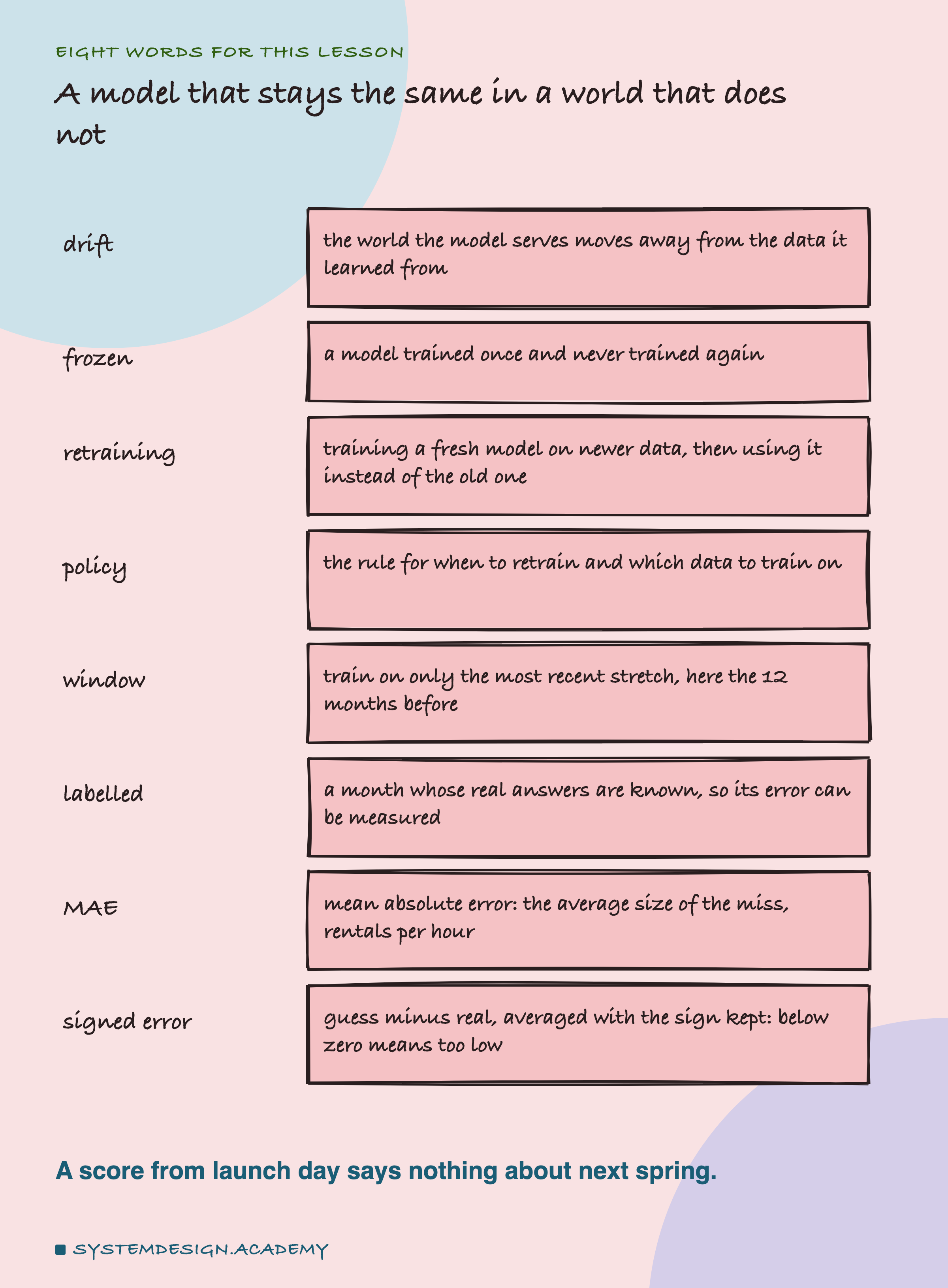
A model is a program that learned from examples to guess a number, here the bikes rented in one hour. Lesson 1 defined it, along with training (showing the model rows where the answer is known) and the mean absolute error, or MAE: for every hour, take the difference between the guess and the real count, drop the minus sign, and average. Its unit is rentals per hour.

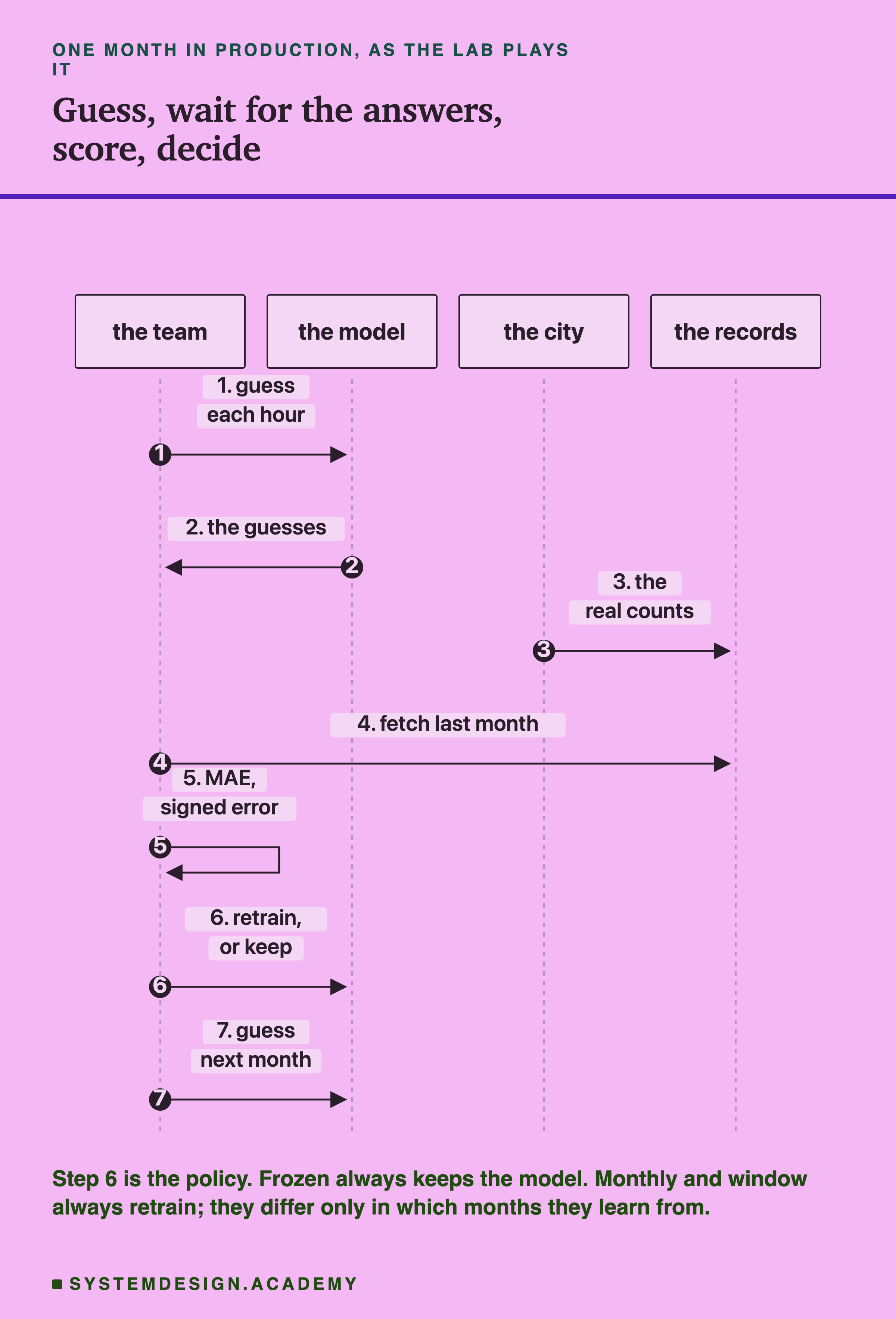
Drift is the name for the world moving away from the data a model learned from. Here the drift is simple and large: many more people rented bikes in the second year. A frozen model is one that is trained once and then used as it is, forever. Retraining means training a fresh model on newer data and putting it in place of the old one. A policy is the rule that says when to retrain and which rows to train on. A window policy trains only on the most recent stretch of time, here the twelve months before the month being guessed, and forgets everything older.

A month is labelled once its real answers are known, so its error can be measured. For bike rentals that happens as soon as the hour is over, because the count is the answer. In many other jobs the answer comes much later: whether a loan is repaid can take years. Last, the signed error is the average of the guess minus the real count, keeping the sign. MAE says how big the misses are. The signed error says which way they lean: below zero means the model guessed too low on average.

Here is the drift in this data, measured, before any model is involved: the average number of bikes rented per hour, month by month, across both years.

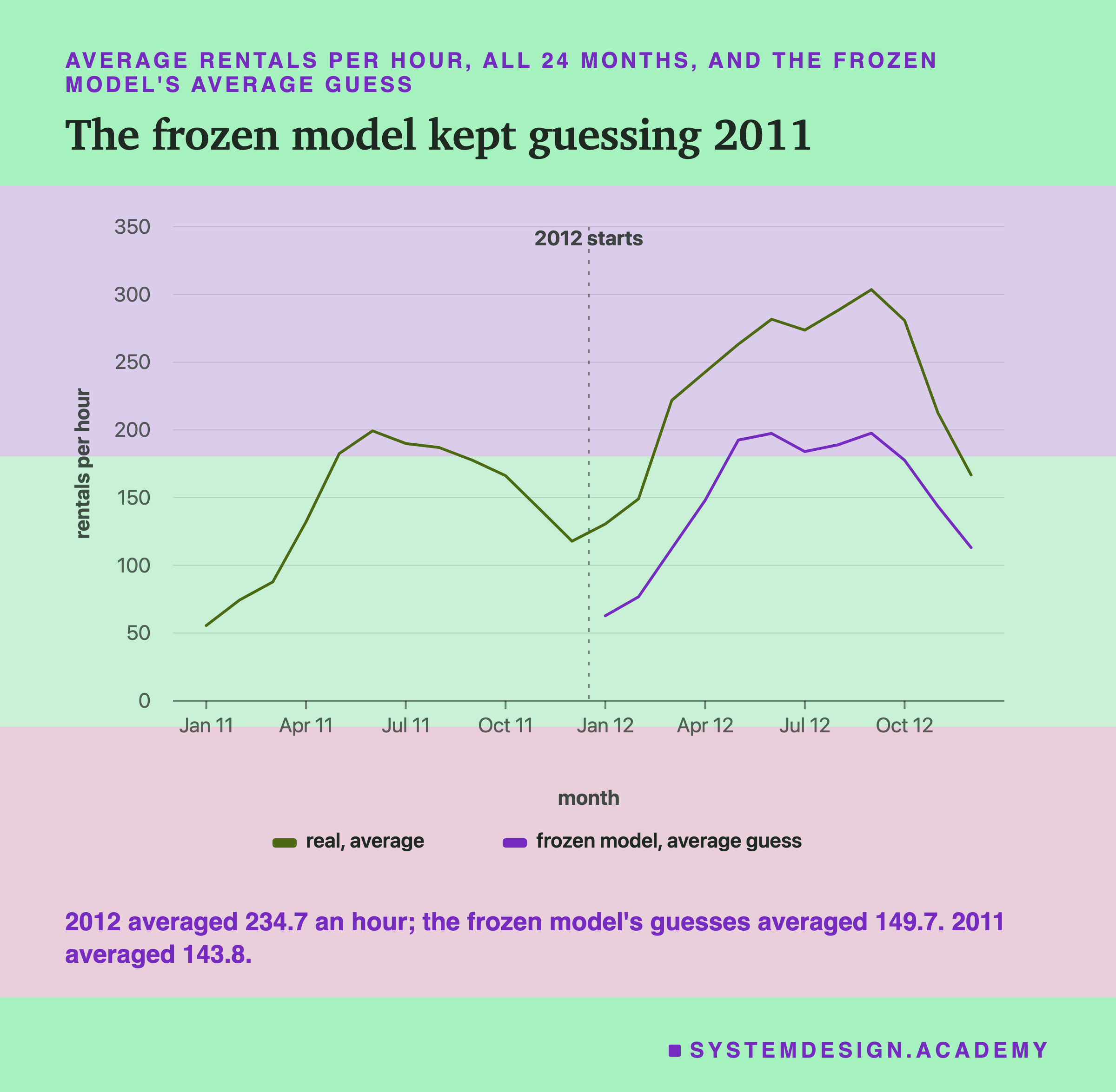
In 2011 the scheme averaged 143.8 rentals an hour. In 2012 it averaged 234.7. Every month of 2012 was busier than the same month of 2011, from 1.41 times (June and December) to 2.53 times (March). Lesson 1 showed the yearly totals; the new thing here is the second line on the chart, which is the model that never learned about 2012. I will come back to it. For now, look at the shape: its guesses for 2012 rise and fall in almost exactly the way 2011 did, at almost exactly 2011's height.

The drift is not only in the level. The lab report also measured how much each month grew over the month before. In 2011, March was 1.18 times February. In 2012, March was 1.49 times February, the largest jump from one month to the next in all of 2012. In 2011, September was already quieter than August (0.95 times). In 2012, September was busier than August (1.05 times). So the second year was not simply the first year multiplied by a fixed number. It was busier, and its busy months came at slightly different times.

Why did the second year grow? The data cannot say. It has no column for the number of docking stations, the number of members, or the price. Growth is common for a new scheme in its second year, but that is my reading, not something this file measures. What the file does measure is that the growth happened, and that a model which learned only 2011 never saw it.

Everything in this lesson compares three policies. Each one answers the same question before every month of 2012: which months should the model learn from?

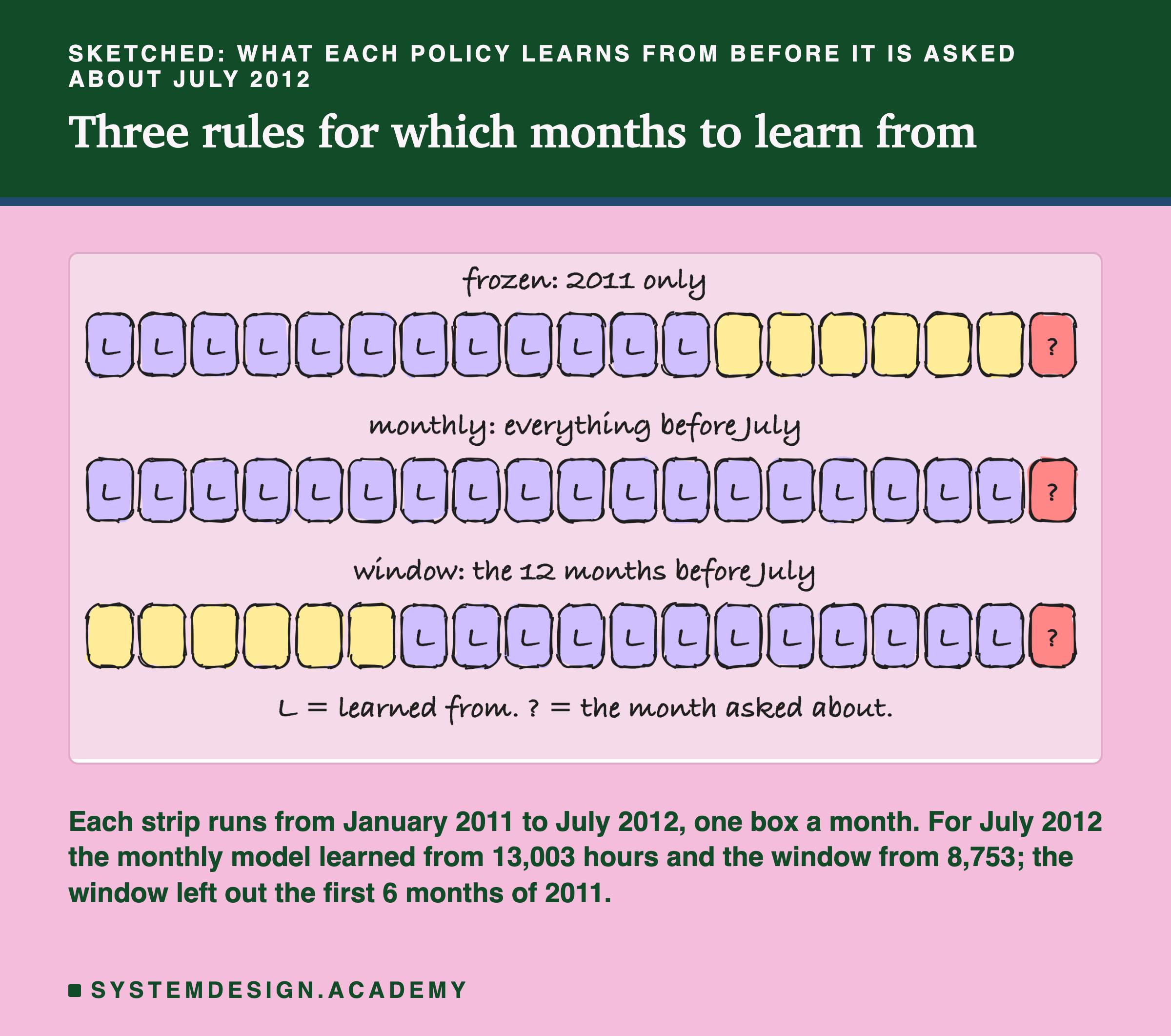
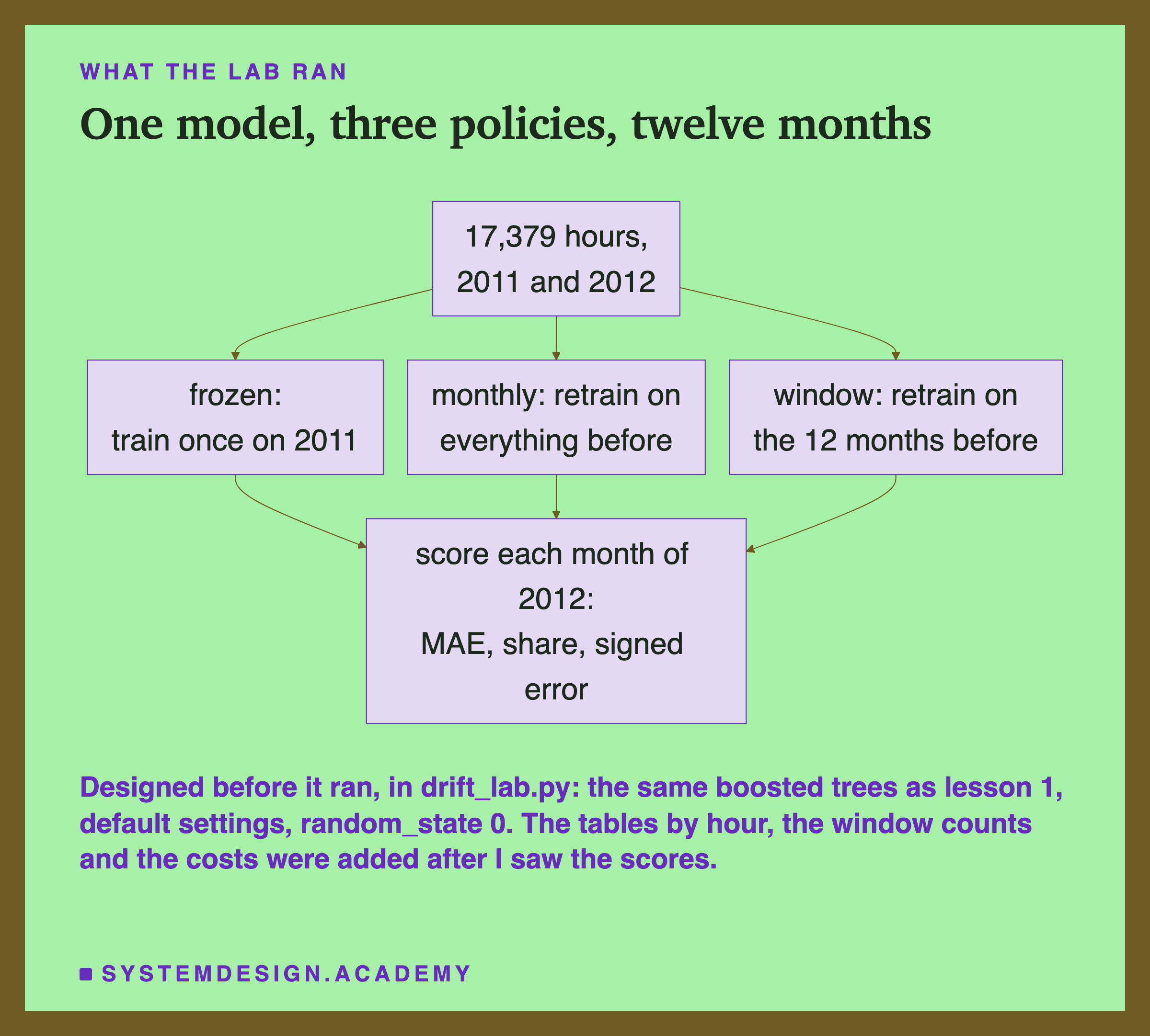
The frozen policy trains once, on all of 2011, and never again. Before July 2012 it still knows only 2011. The monthly policy retrains before every month on everything before that month: before July 2012 that is all of 2011 and the first six months of 2012, 13,003 hours. The 12-month window policy also retrains before every month, but only on the twelve months just before it: before July 2012 that is July 2011 to June 2012, 8,753 hours. It throws away the first six months of 2011.

Each policy has a reason behind it. Frozen is the cheapest: one model, trained once, nothing to maintain. Monthly uses every example there is, on the idea that more data is better. The window uses only recent data, on the idea that the old months describe a world that no longer exists. Which idea wins depends on the data, and the lab measured it on this data only.

In every case the model for a month never sees any hour of that month while it learns. The test is always the future, like the forward split of lesson 1, only repeated twelve times.

I wrote the design at the top of the lab file, drift_lab.py, before I ran it: the question, the data, the model, the three policies, the months to score, and the four numbers to store for each month and policy. The dated record is the chapter plan, CHAPTER-PLAN.md (2026-09-29, "DRIFT LAB (batch 2) designed before running"). The design also says, in writing, that there is no test of significance (a calculation of how likely a difference this large would be to appear by luck alone): this is one year and one run per policy, a description and not an experiment that can prove one policy better than another in general.

The model is the same as in lesson 1: scikit-learn's HistGradientBoostingRegressor, which I call boosted trees, with its default settings and random_state=0, a fixed seed so that the same data always gives the same model. It learns by building many small decision trees, each one asking yes-or-no questions about the inputs and each one correcting the mistakes of the ones before. I did not tune it. The same 12 inputs go in: season, year, month, hour, holiday, day of the week, working day, weather, temperature, "feels like" temperature, humidity and wind speed.

The months. Month number 1 is January 2011 and month 24 is December 2012. For each of the twelve months of 2012, and for each policy, the lab chose the training rows by the policy's rule, trained a fresh model, and asked it about every hour of that month: 8,734 hours in all. It stored four numbers per month and policy (the MAE, the real average for the month, the MAE as a share of that average, and the signed error) and, for every hour, the guess itself.

The MAE from lesson 1 has one weakness for this lesson: it cannot tell you whether a model guesses too high or too low. A model that is 70 too low every hour and a model that is 70 too high half the time and 70 too low the other half have the same MAE. They need very different fixes. So this lesson adds a second score. Lesson 1 already had it and called it the bias (its forward test's overall bias was -11.2); here I call it the signed error.

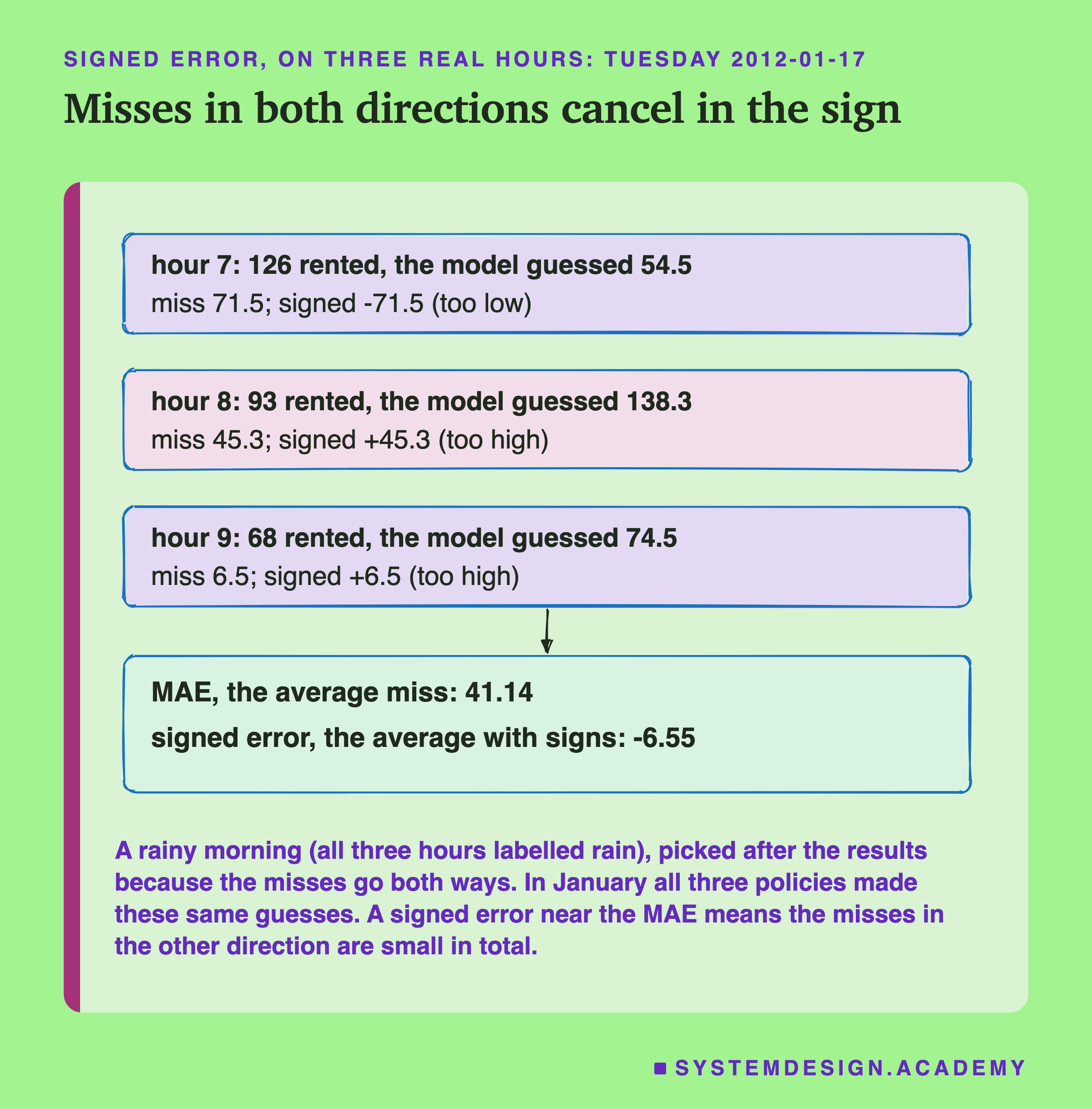
These are three real hours from Tuesday 17 January 2012, the morning rush on a rainy morning (all three hours are labelled rain). I picked them (after the results) because they go both ways, which is uncommon in this lesson. At 7 in the morning 126 bikes were rented and the model guessed 54.5: 71.5 too low. At 8, 93 were rented against a guess of 138.3: 45.3 too high. At 9, 68 against 74.5: 6.5 too high. The MAE of the three is 41.14. The signed error is the plain average of the three differences, -71.5, +45.3 and +6.5, which is -6.55. The misses were big, but they partly cancelled.

That is how to read the two together. When the signed error is close to zero, the misses go both ways and the model is not leaning. When the signed error is almost as large as the MAE, with a minus sign, the misses that were too high add up to very little: they may not be rare, but they are small next to the misses too low. The model is guessing a smaller world than the real one. The gap between the two numbers tells you how one-sided the misses are, and a one-sided miss is the typical sign of the kind of drift in this lesson.

One more measure from lesson 1 comes back here: the MAE as a share of the month's real average. A miss of 40 in a month that averages 130 rentals an hour is worse than a miss of 40 in a month that averages 300. The share puts the months on one scale.

Here is the headline, from the lab's stored file, results/drift.json.

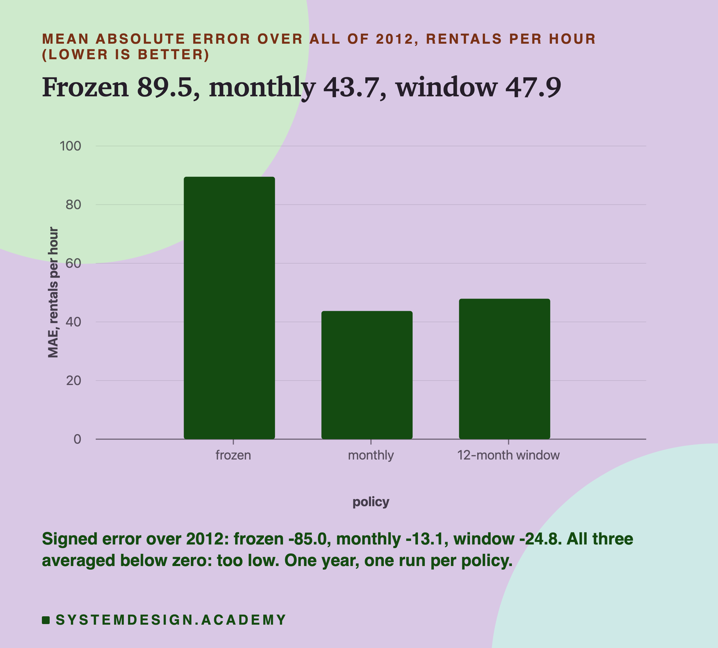
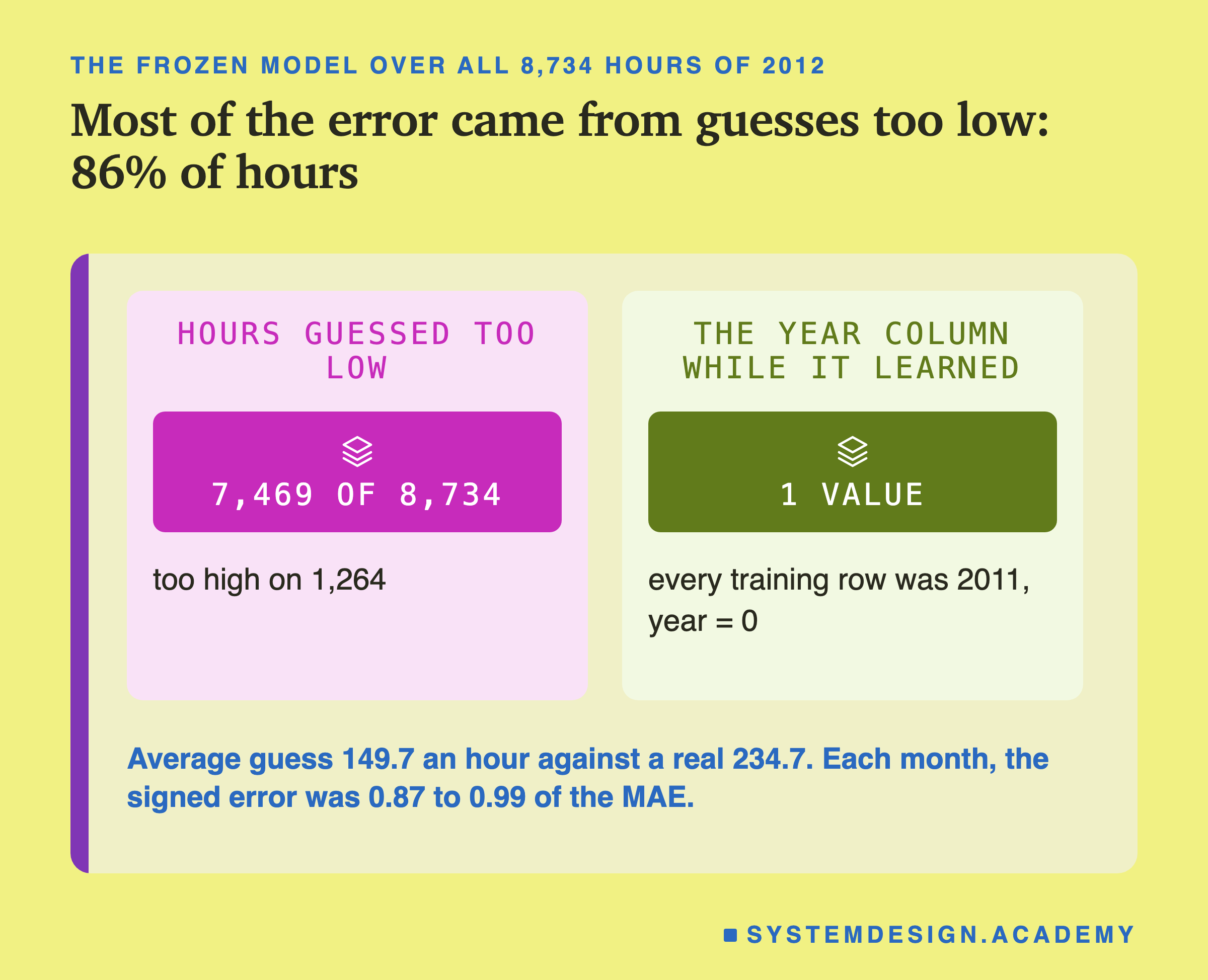
Over all 8,734 hours of 2012, the frozen model missed by 89.5 rentals an hour on average, with a signed error of -85.0. The monthly policy missed by 43.7, signed -13.1. The 12-month window missed by 47.9, signed -24.8. The frozen model's signed error is almost as large as its MAE: most of its error came from guessing too low. Retraining every month cut the average miss roughly in half here, and the lean fell from -85.0 to -13.1. A later slide shows what made that possible.

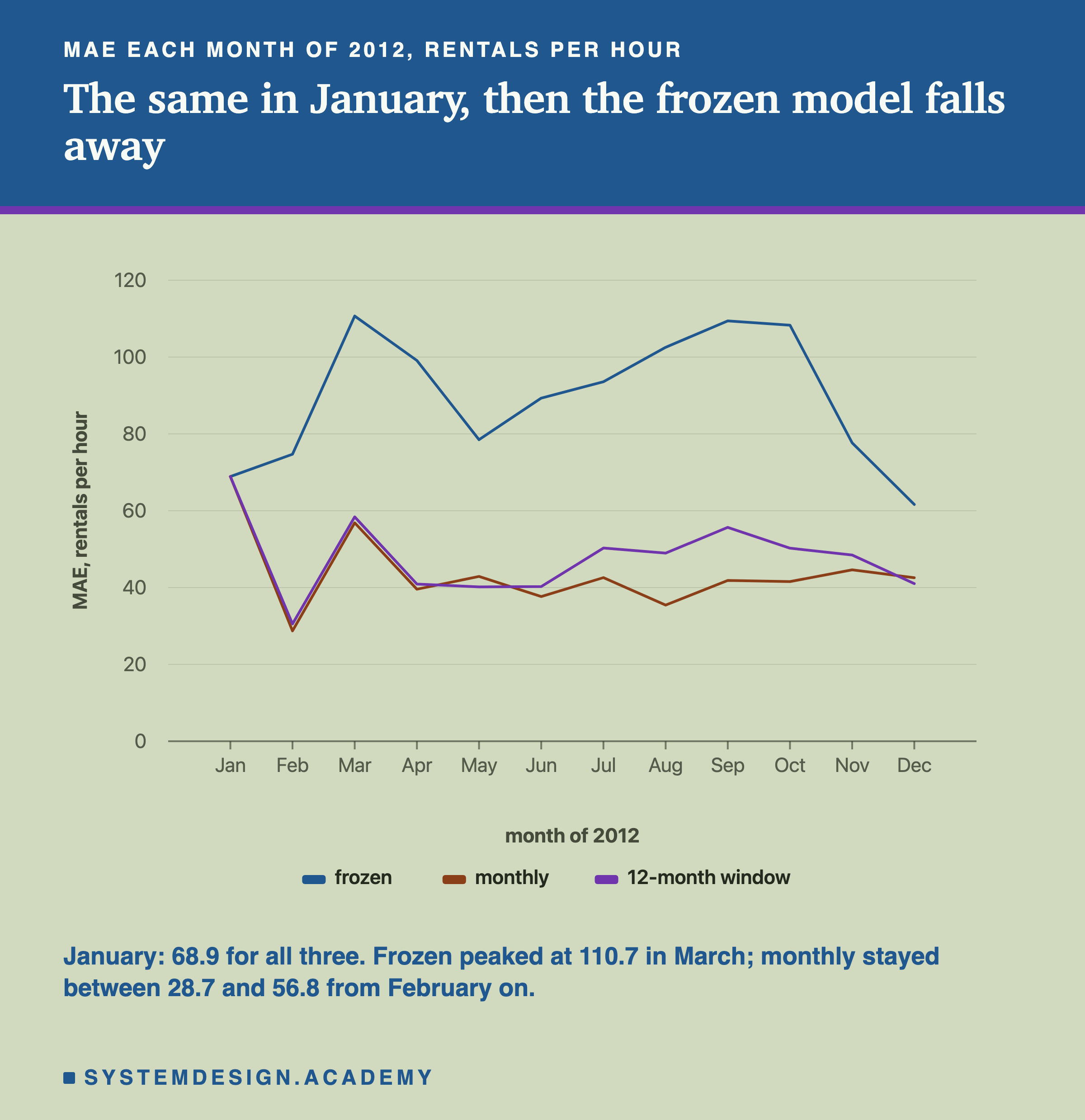
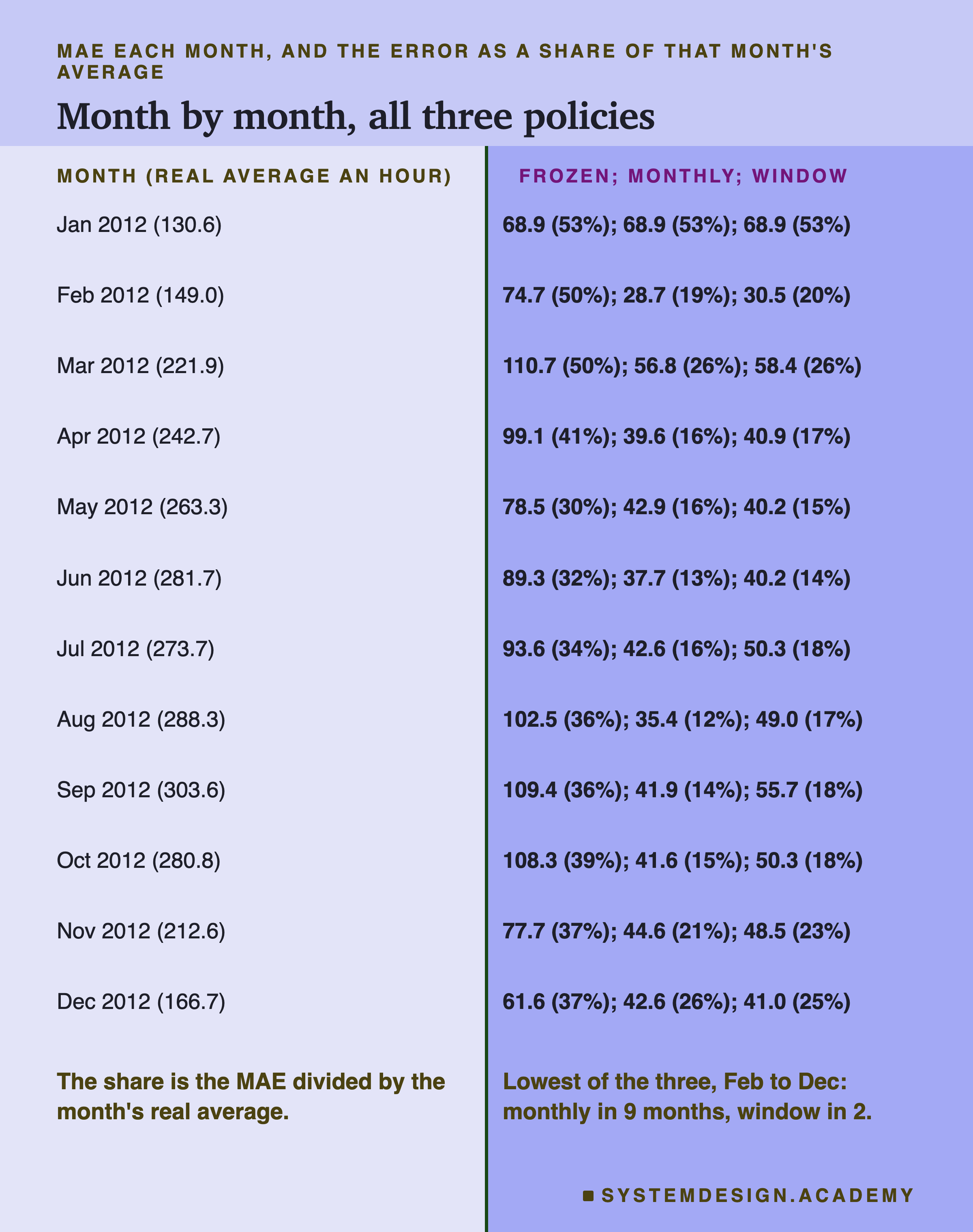
Month by month, the three policies start at exactly the same place. In January 2012 all three missed by 68.9, because all three had learned from 2011 only. There was nothing else yet. From February the retrained models had one month of 2012 to learn from, and their error dropped to 28.7 (monthly) and 30.5 (window), while the frozen model's rose to 74.7. After that, the frozen model's error stayed between 61.6 and 110.7 for the rest of the year, and the monthly policy's stayed between 28.7 and 56.8.

The frozen model was not just wrong. It was wrong in one direction, month after month.

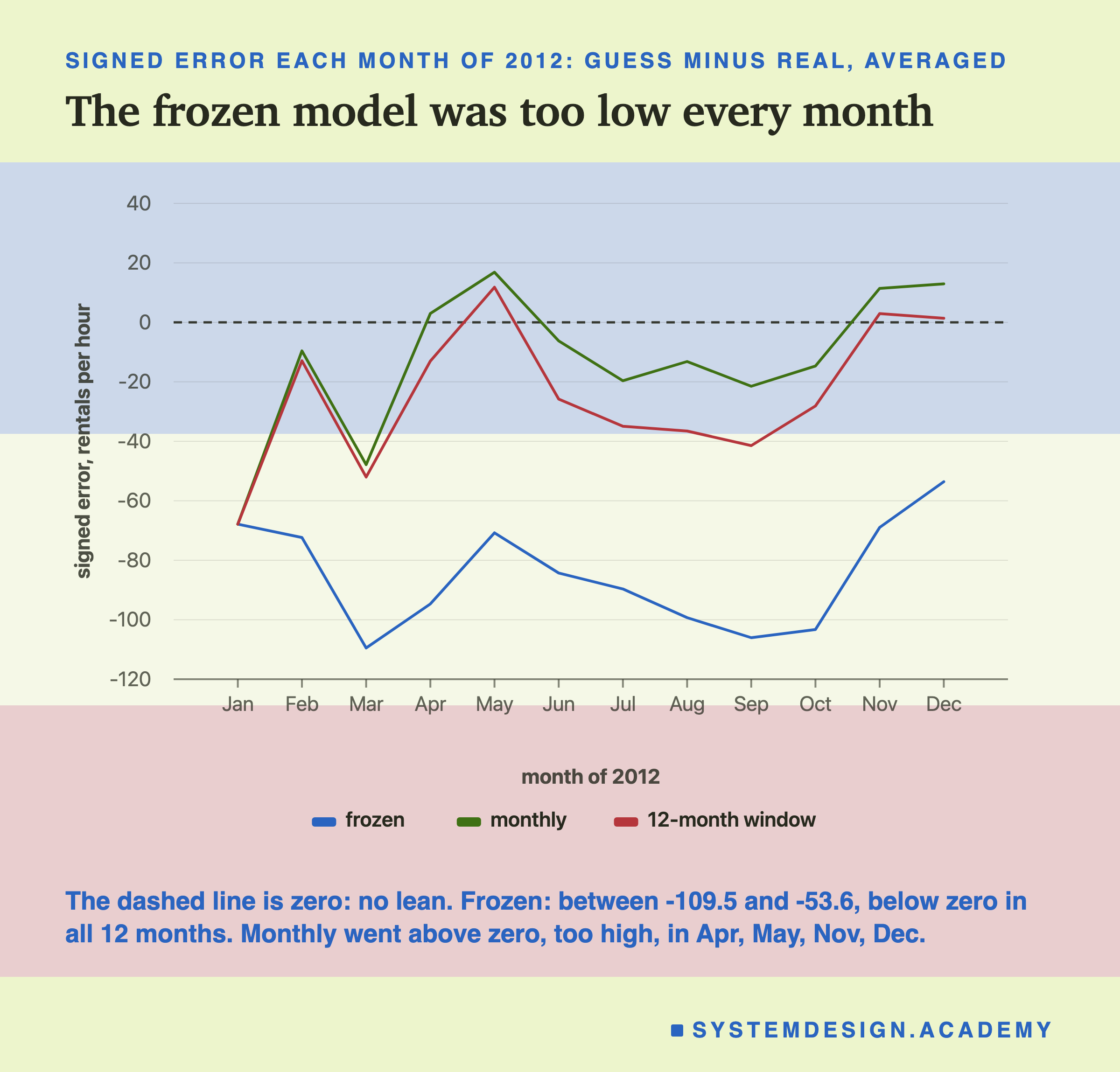
Its signed error was below zero in all twelve months, from -53.6 in December to -109.5 in March. In every month the size of the signed error was between 0.87 and 0.99 of the MAE: the misses too high were small in total. By count, it was too low on 7,469 of the 8,734 hours (86%); even in December, its best month, it was too low on 582 of 742. The retrained models lean much less. The monthly policy even went above zero, guessing too high on average, in April, May, November and December.

So what was the frozen model guessing? The lab report compared its average guess for each month of 2012 with the real average of the same month in 2011. (After the results.)

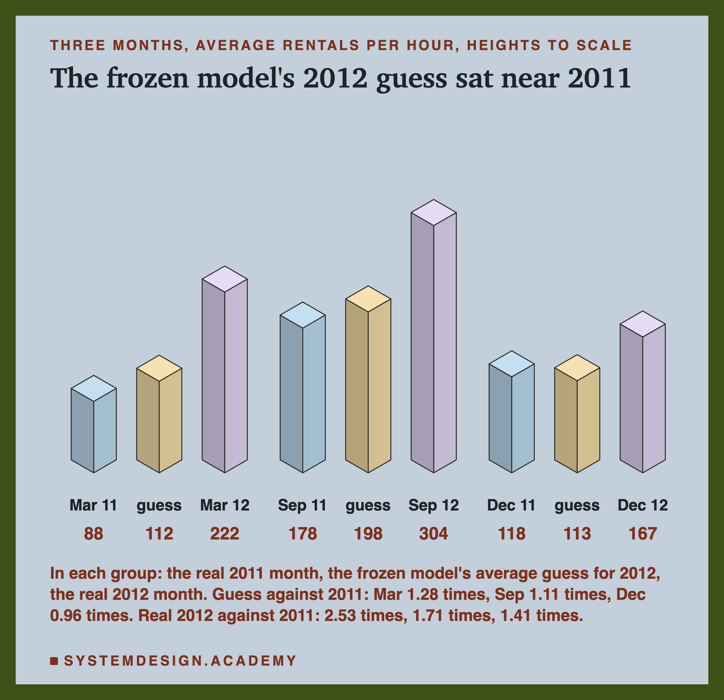
The answer is plain: it guessed last year. Across the twelve months, its average guess for a 2012 month was between 0.96 and 1.28 times the real 2011 average for that month. The real 2012 months were between 1.41 and 2.53 times their 2011 averages. Over the whole year it guessed 149.7 rentals an hour on average, close to 2011's 143.8, while 2012 really averaged 234.7.

The lab stored every hour's guess, so the misses can be sorted by the hour of the day. I read these tables before writing about them (after the results).

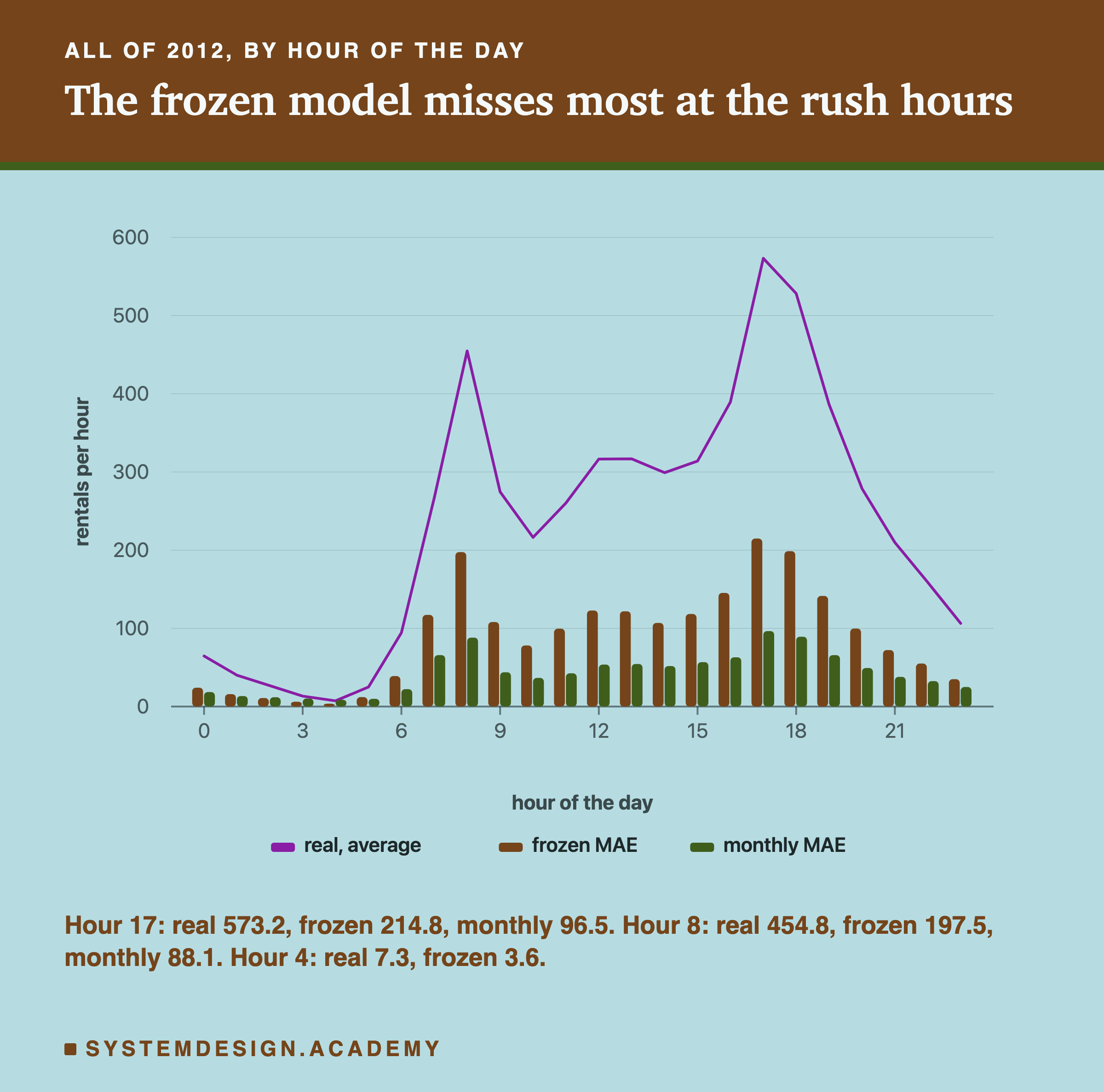
The biggest misses are at the commuting peaks. At hour 17, when the real average was 573.2 rentals, the frozen model missed by 214.8 and the monthly model by 96.5. At hour 8, real 454.8, the frozen model missed by 197.5 and monthly by 88.1. As a share of each hour's average, the frozen model missed these three peak hours by about 37% to 43% and monthly by about 17% to 19%. The busy hours grew the most in absolute numbers, and a model that expects last year's crowd misses them the most.

The quiet hours tell a small surprise. At hour 4, when about 7 bikes an hour were rented, the frozen model missed by 3.6 and the monthly model by 8.7. At hours 2, 3 and 4 the monthly model's miss was larger than the frozen model's (11.9 against 10.8, 10.2 against 6.2, 8.7 against 3.6), and at hours 3 and 4 its signed error was above zero (+4.9 and +6.9): it guessed too many bikes in the middle of the night. One possible reason, a guess: a retrained model learned that 2012 was busier, and applied some of that growth to hours that grew little. Those hours hold very few bikes, so this costs little in total, but it is a reminder that retraining does not improve every slice.

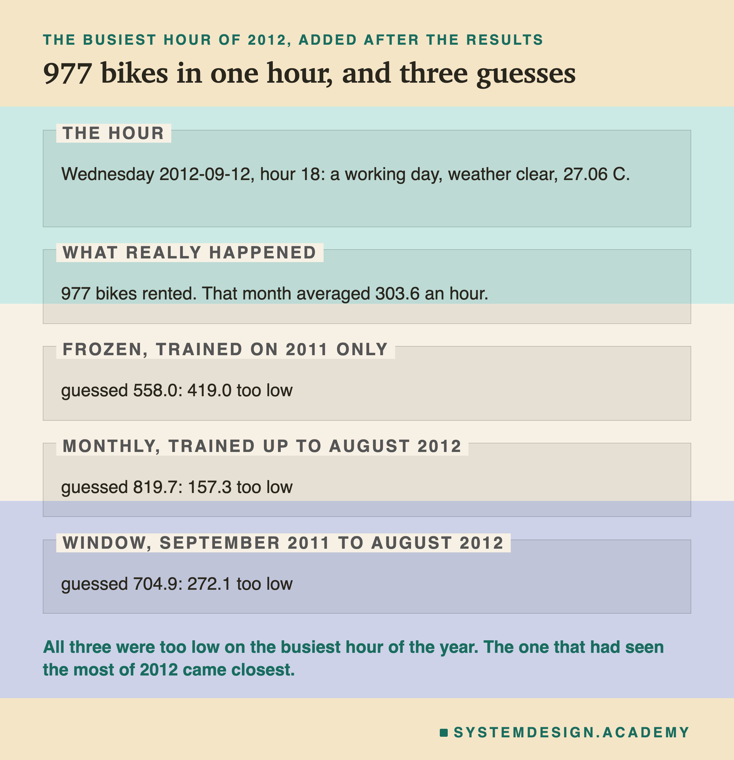
One hour shows the pattern in a single row. The busiest hour of 2012 was 6 in the evening on Wednesday 12 September, a clear working day at 27.06 C, when 977 bikes were rented (the date is rebuilt from the day-of-week column, as in lesson 1). The frozen model guessed 558.0, 419.0 too low: a big evening for 2011, not for 2012. The 12-month window guessed 704.9, and the monthly model, which had learned from every hour up to the end of August 2012, guessed 819.7, still 157.3 too low. I picked this hour (after the results) because it is the largest count of the year; it is one hour, not a summary, but it shows how far behind a model that learned last year's crowd can be on the day the new crowd is biggest.

I expected the 12-month window to do at least as well as monthly retraining. The world was changing, so forgetting the oldest months sounded sensible. It did worse in 9 of the 11 months after January. Before guessing why, I looked at what the window actually leaves out (after the results).

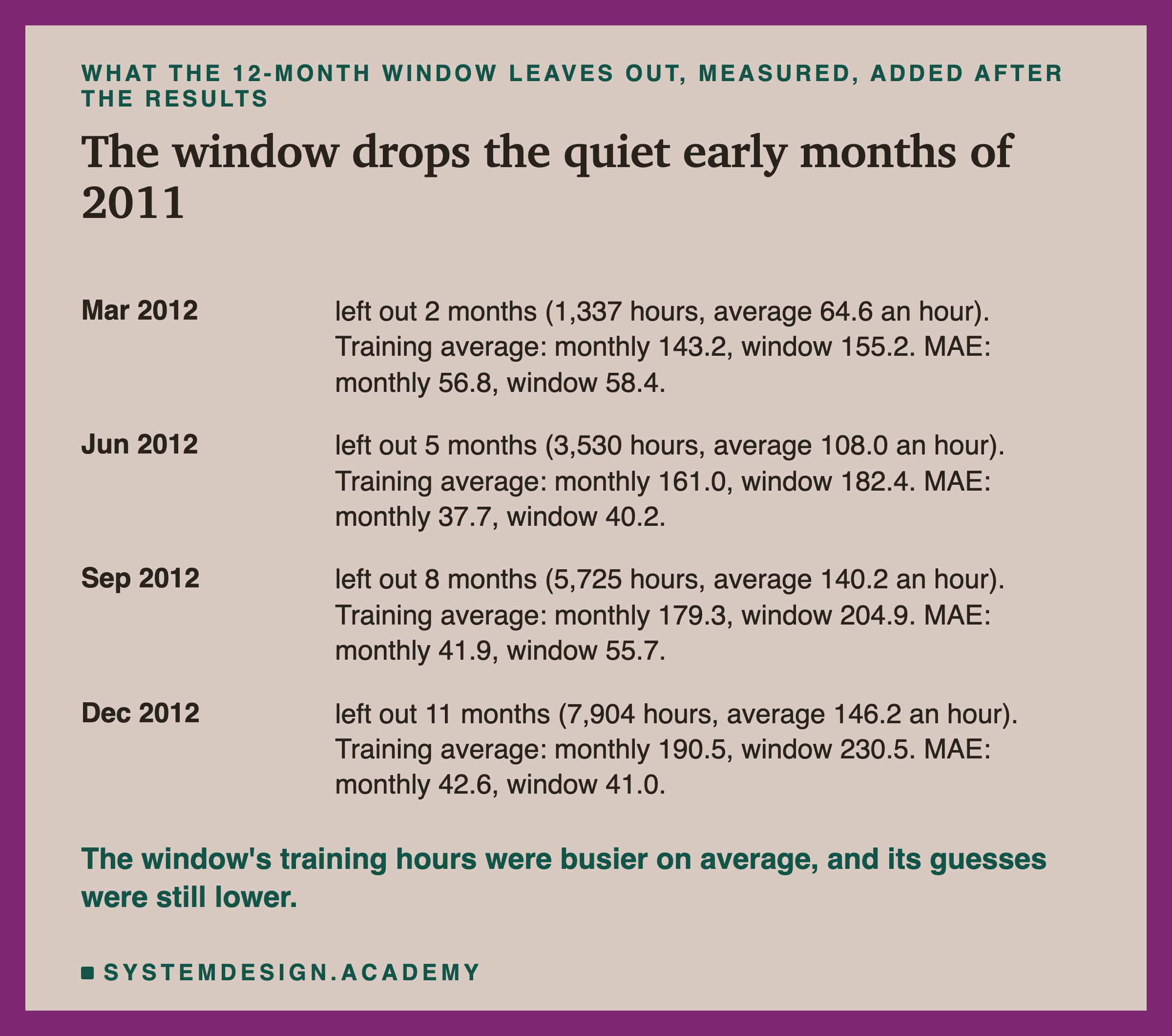
The window drops the oldest months of 2011, which were the quietest months in the whole dataset. Before September 2012, for example, it left out eight months, 5,725 hours averaging 140.2 rentals an hour. So the window's training hours were busier on average than the monthly policy's: 204.9 against 179.3 an hour before September. You might expect busier training data to push the guesses up. It did not. The window's signed error was below the monthly policy's in all 11 months from February to December. Its guesses were lower, not higher.

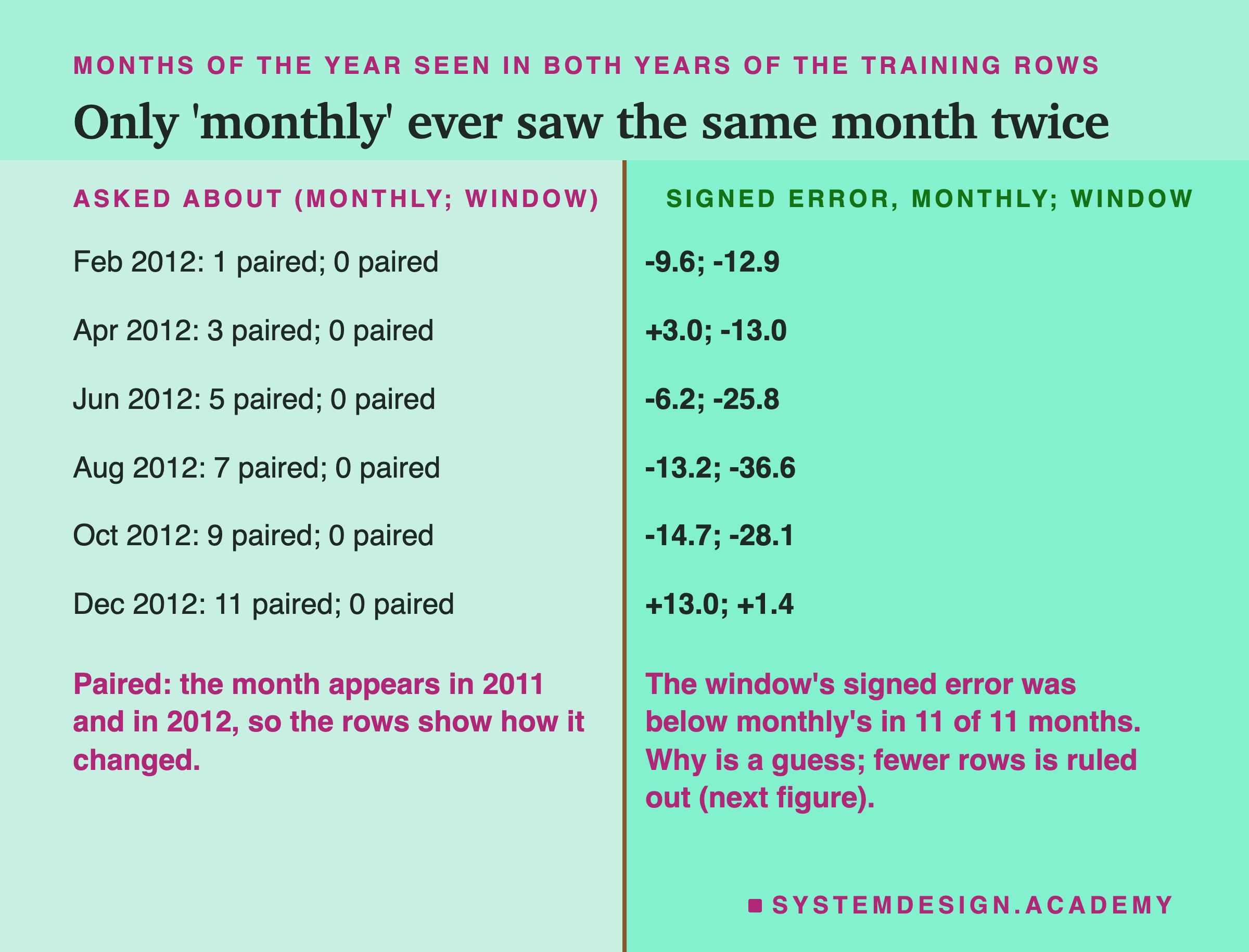
Here is the one other thing the report measured. Call a month of the year paired in a set of training rows if that month appears from both years: say, January 2011 and January 2012. Paired months are the only rows that show the model how the same month changed from one year to the next. Before June 2012, the monthly policy's training rows held 5 paired months (January to May of both years). The window held 0. It always holds 0, because twelve months in a row contain each month of the year exactly once. A concrete case: in the window used before September 2012, the 2012 rows are January to August, and the 2011 rows are September to December. So in that window, "year = 1" also means "early in the year", and "year = 0" also means "late in the year".

A review of this lesson asked a question I had not: did retraining help because of the fresh rows, or because of one particular input? So I added a follow-up to the lab, designed after the main results and prompted by that review. Its design is the docstring of the lab's followup mode, and its results are in results/drift_followup.json. It reruns the three policies from February to December 2012 (January is the same for all three) with one change: the year column is made constant, so no tree can use it. Everything else is the same: the months, the rows, the model, the seed.

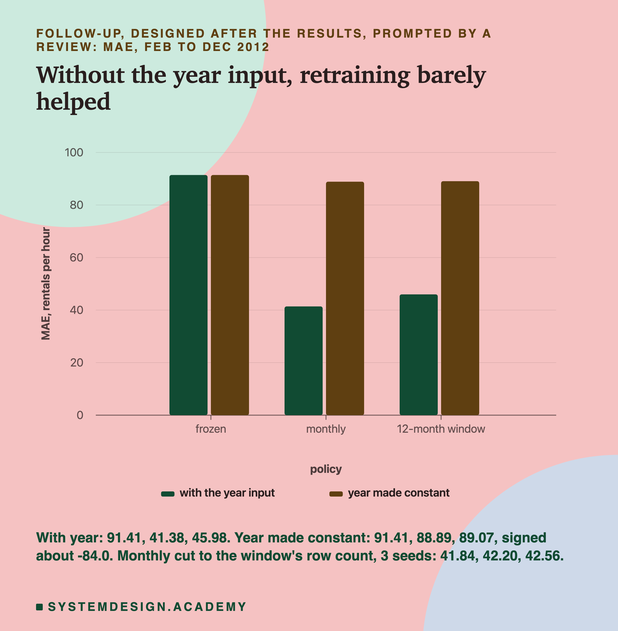
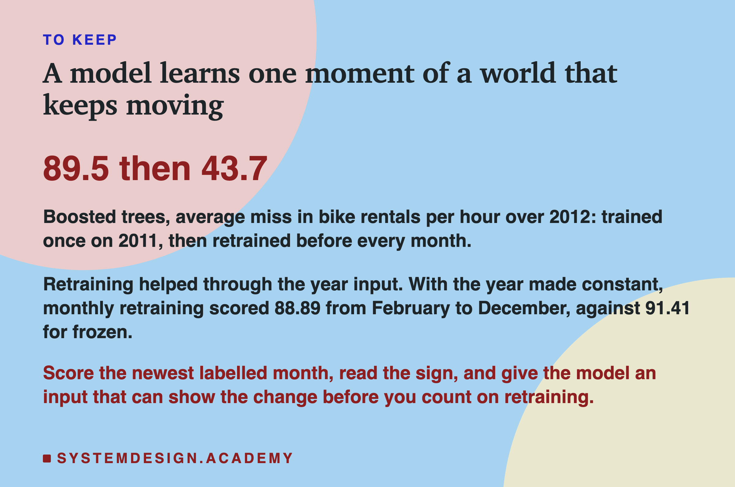
With the year as an input, the three policies scored 91.41, 41.38 and 45.98 from February to December. With the year made constant, they scored 91.41, 88.89 and 89.07. The frozen model did not change at all, which fits the measurement on the earlier slide: it never used the year. The two retrained models lost almost all of their advantage. Monthly retraining, which had every row of 2012 up to the month before, missed by 88.89, only a little better than never retraining, and its signed error was -84.0, against -8.1 with the year. It kept the lean.

This changes the lesson's main advice, and I want to be plain about it. Retraining on newer rows is not, on its own, a fix for a world that has changed. Here it worked because the model had an input that could say "this row is from the new world": the year. With that input, fresh 2012 rows taught the trees that 2012 sat above 2011. Without it, the fresh rows were mixed with the old ones under the same month, hour and weather, and the model went on guessing close to the old level. Why the trees averaged the two years in that way is my reading; that the lean stayed is measured.

The same follow-up tested the window's row count. The monthly policy, cut at random to the window's number of training rows for each month, scored 41.84, 42.20 and 42.56 over three seeds, all well under the window's 45.98. So the window did not do worse only because it had fewer rows. This is one run per setting on one year, and designed after the results; read it as a strong hint about this data, not a rule.

Retraining learns from the past. However often you do it, there are two things it cannot do, and the data shows both.

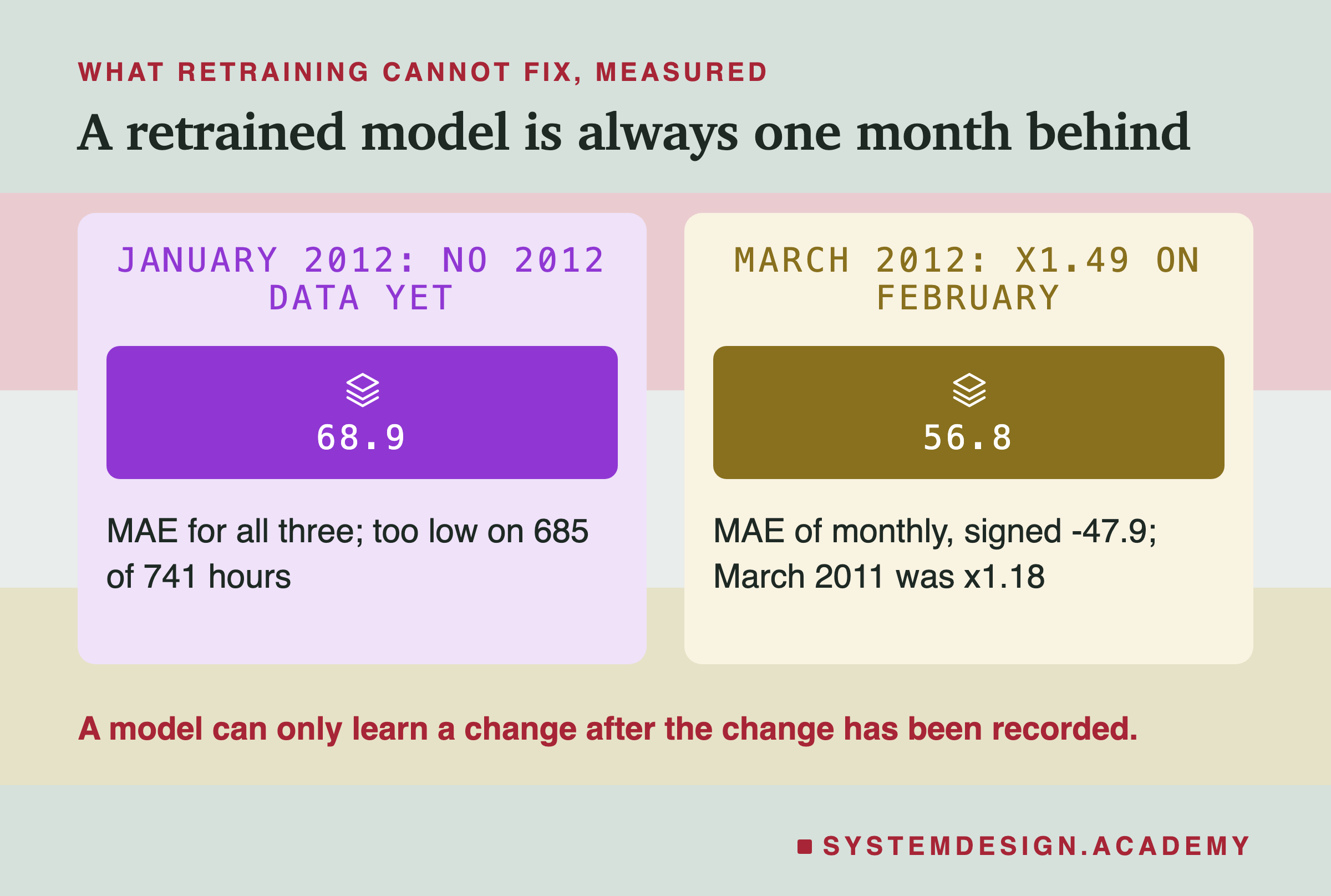
The first month after a change. In January 2012, all three policies had exactly the same model, trained on 2011 only, because no hour of 2012 existed yet. The largest difference between their January guesses was 0.00. All three missed by 68.9 and guessed too low on 685 of the 741 hours. No policy can do better on the first stretch after a change, because the change has not been recorded yet. The only defences are outside the model: someone who knows that a new year is expected to be busier, or a warning from inputs that look different, which a later lesson in this chapter is planned to measure.

A sudden jump inside the year. In 2012, March was 1.49 times as busy as February, the largest jump from one month to the next that year. In 2011 the same step was only 1.18 times. The monthly policy, retrained on everything up to the end of February, missed March by 56.8, with a signed error of -47.9, its worst month after January. It had learned February 2012; it could not know how much bigger March would be until March was over. In April, once March was in its training rows, its miss fell to 39.6.

So even the best policy here is always about one month behind. Retraining more often, every week or every day, would shorten the delay, but it cannot remove it, and it costs more, which is the subject of a later slide. A retrained model learns what already happened. It is a way to catch up, not a way to see ahead.

In real use you do not get a table for the whole year. At the start of each month, you know one new thing: how the model did on the month that just ended, because its real answers have arrived. That is the newest labelled month, and it is the number to decide on. I added this reading of the results afterwards.

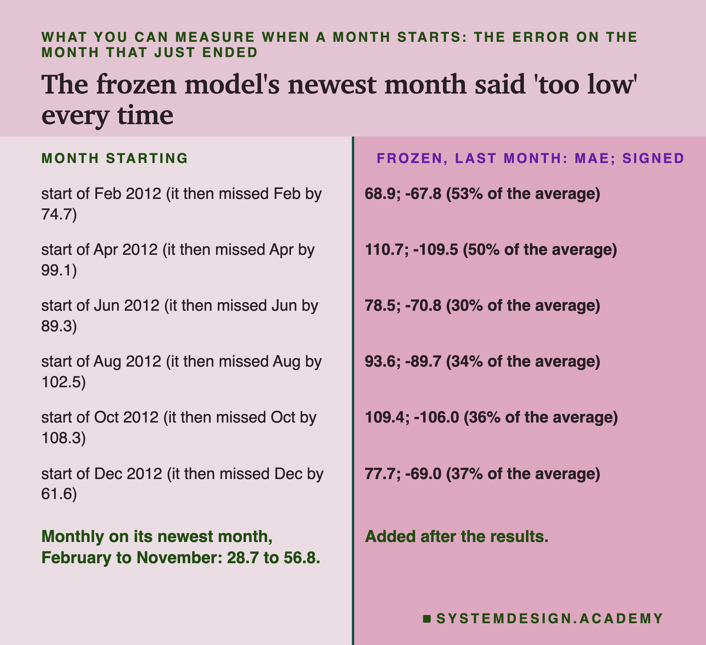
Suppose you had shipped the frozen model and were watching it. At the start of February 2012, January's answers are in. January's MAE was 68.9, which is 53% of January's average, and its signed error was -67.8: most of the error came from guesses too low (it was under the real count on 685 of 741 hours). That one number, read on the first day of February, already says what the rest of the year will show: this model expects a smaller world than the real one. Every month after that tells the same story, from 30% to 50% of the month's average, always with the minus sign.

How would you decide? You need a line to compare with. The honest line is the error you accepted when you shipped the model, measured with a forward test like lesson 1's (train on the past, score the stretch after it): if the model scored about 15% of the average in testing and the newest month shows 53%, something has changed. The retrained models give a feel for the range here: after January, the monthly policy's newest month was between 28.7 and 56.8, 12% to 26% of each month's average. A frozen model reading 50% is far outside that.

Then read the sign. A newest month whose signed error is almost as large as its MAE means the misses lean one way, which points at a change in level: the whole world got busier or quieter, not just noisier. That is the kind of drift in this lesson. It tells you the model is behind; it does not yet tell you that retraining will catch it up. The next slide shows that here, retraining caught up only because the model had an input, the year, that could express the change. A large MAE with a signed error near zero means the misses go both ways: the model is noisy, not behind, and retraining on more of the same may not help. The exact line where you act is a choice for your job. This lab did not test any particular line, so I do not give one as if it were measured.

Retraining is not free, and the cheapest policy was the frozen one. The lab report counted what each policy had to do over 2012 (after the results).

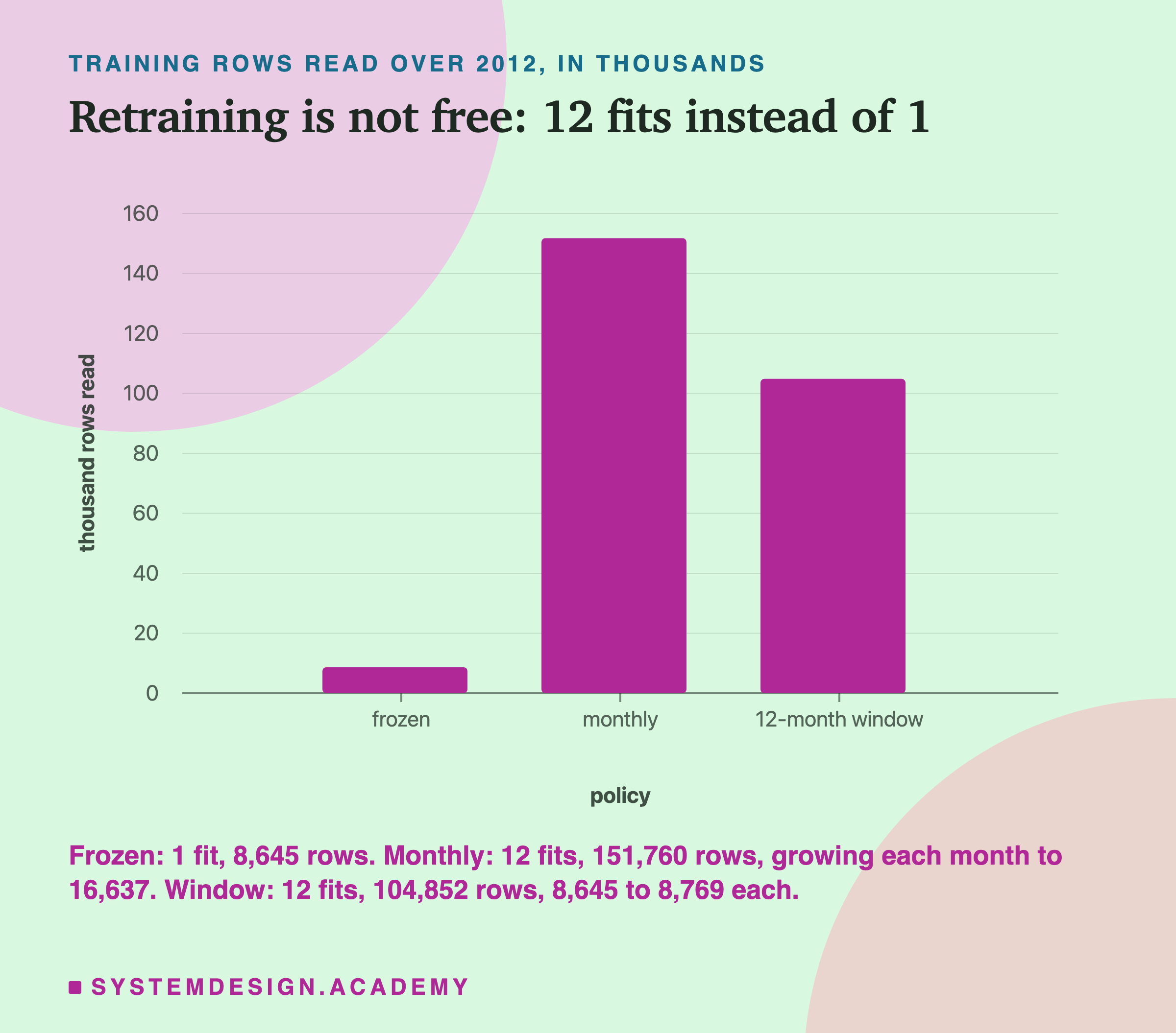
The frozen policy trains once, on 8,645 hours. The monthly policy trains 12 times, and each time on more rows than before, from 8,645 in January to 16,637 in December: 151,760 rows read in total. The window policy also trains 12 times, but each time on about a year of rows, between 8,645 and 8,769: 104,852 in total. So monthly retraining read about 17.6 times as many rows as the frozen model, and the window about 12.1 times.

I did not time the fits, so I report rows, not seconds. On a model trained on millions of rows, or on a large language model, the cost of each retrain is real money and real time, and the monthly policy's cost keeps growing with the data while the window's stays flat. That flat cost is one honest reason to choose a window even when it is a little less accurate.

The rows are not the only cost. Every new model is a new thing in production. Someone should check it before it replaces the old one: score it on a forward test, compare it with the model it replaces, and keep the old one ready in case the new one is worse. Twelve retrains a year means twelve of those checks. A policy that retrains often without checking has swapped one risk (a model that grows old) for another (a bad new model that nobody looked at).

Lesson 1 had one forward split: a model trained on everything up to hour 11 of a day in August 2012, then scored on the rest of 2012. That is a frozen model too, just frozen later. I put its monthly errors next to the monthly policy's (after the results).

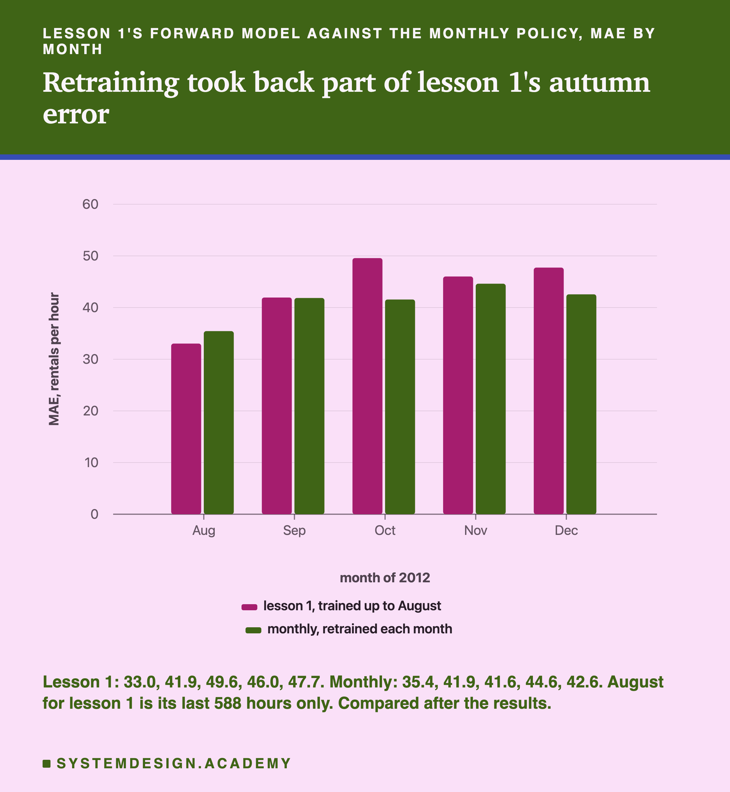
September is the check. Lesson 1's model and the monthly model for September trained on almost the same rows: everything up to August 2012, except that lesson 1's model stopped partway through August. They missed September by 41.94 and 41.85: close, as expected from nearly the same training rows. Two separate labs, run in two separate files, agree where they should. From October on, the monthly policy had seen September, and then October, and so on, while lesson 1's model had not. Its errors were 49.6, 46.0 and 47.7 for October to December; the monthly policy's were 41.6, 44.6 and 42.6.

August looks like the exception, 33.0 against 35.4, but it is not a fair pair: lesson 1's August holds only its last 588 hours, the stretch just after its training ended, while the monthly policy's August is the whole month, scored by a model that had seen no August at all. Different hours, different questions.

This joins the two lessons into one picture. Lesson 1 said: test on the future, or your score is too kind. This lesson adds: the future keeps arriving, and a model scored honestly on launch day grows older every month. Lesson 1's forward score, 44.07, was the score of a model on its first four and a half months. The frozen model here shows what the same kind of model looks like after a whole year of not learning.

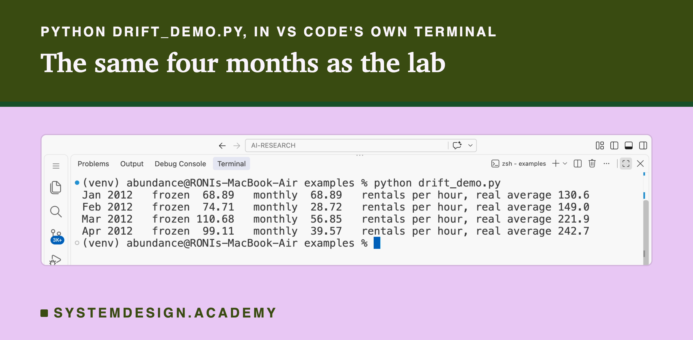
This script is the lab made small. It downloads the same data, trains the frozen model once on 2011, then for January to April 2012 trains a fresh monthly model on everything before each month, and prints both errors for each month. It does not need a GPU.

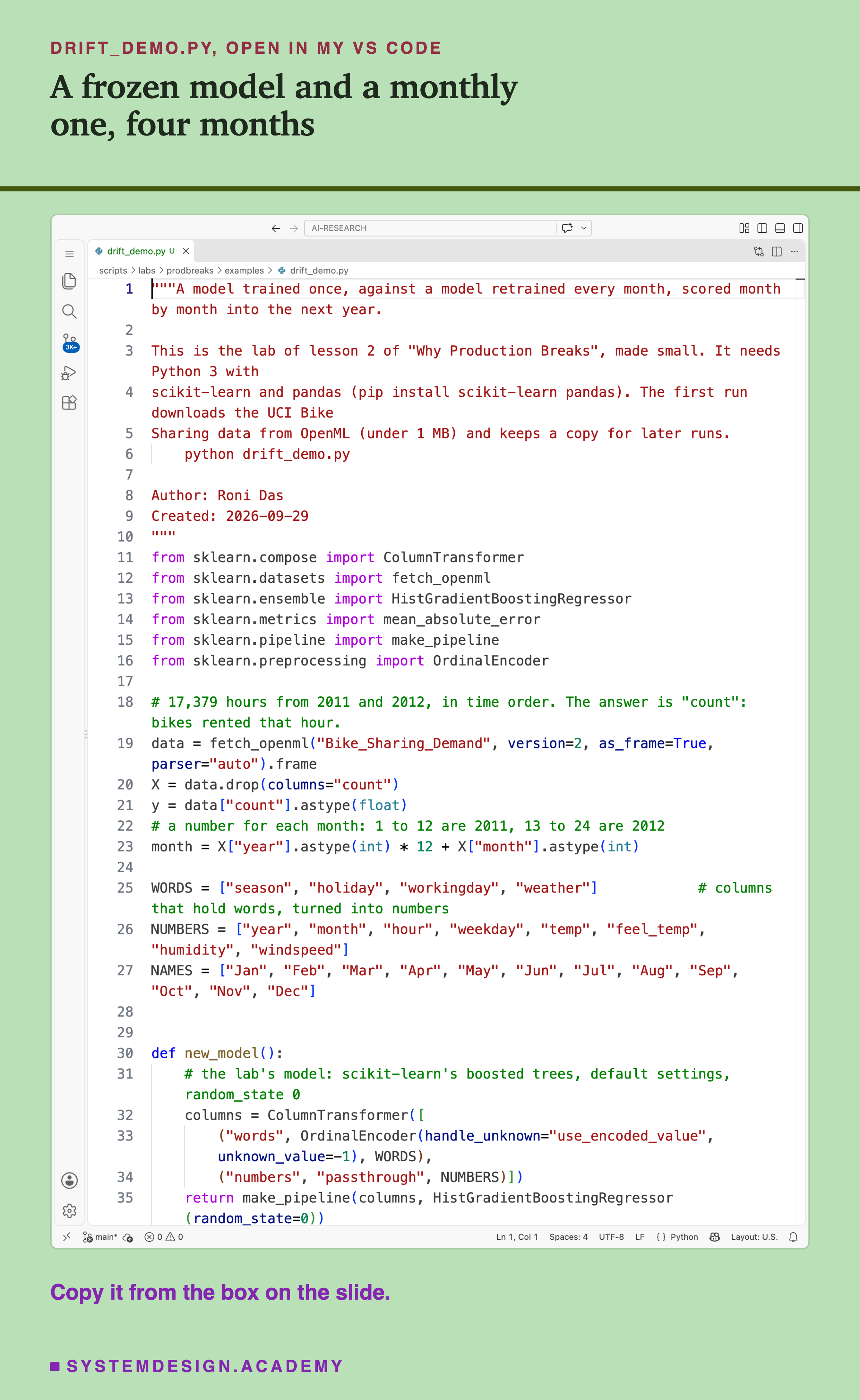
Before you run this lab. You need Python 3 and two libraries: pip install scikit-learn pandas. scikit-learn holds the model, the scores and the download; pandas holds the table. The first run downloads the Bike Sharing data from OpenML, so it needs an internet connection once; scikit-learn keeps a copy in a folder in your home directory (scikit_learn_data) for later runs. I ran it with scikit-learn 1.9.1 on a Mac. scikit-learn runs the same way on Windows and Linux, but I have not checked the numbers there, and another version of scikit-learn may give slightly different decimals.

"""A model trained once, against a model retrained every month, scored month by month into the next year.

This is the lab of lesson 2 of "Why Production Breaks", made small. It needs Python 3 with
scikit-learn and pandas (pip install scikit-learn pandas). The first run downloads the UCI Bike
Sharing data from OpenML (under 1 MB) and keeps a copy for later runs.
    python drift_demo.py

Author: Roni Das
Created: 2026-09-29
"""
from sklearn.compose import ColumnTransformer
from sklearn.datasets import fetch_openml
from sklearn.ensemble import HistGradientBoostingRegressor
from sklearn.metrics import mean_absolute_error
from sklearn.pipeline import make_pipeline
from sklearn.preprocessing import OrdinalEncoder

# 17,379 hours from 2011 and 2012, in time order. The answer is "count": bikes rented that hour.
data = fetch_openml("Bike_Sharing_Demand", version=2, as_frame=True, parser="auto").frame
X = data.drop(columns="count")
y = data["count"].astype(float)
# a number for each month: 1 to 12 are 2011, 13 to 24 are 2012
month = X["year"].astype(int) * 12 + X["month"].astype(int)

WORDS = ["season", "holiday", "workingday", "weather"]            # columns that hold words, turned into numbers
NUMBERS = ["year", "month", "hour", "weekday", "temp", "feel_temp", "humidity", "windspeed"]
NAMES = ["Jan", "Feb", "Mar", "Apr", "May", "Jun", "Jul", "Aug", "Sep", "Oct", "Nov", "Dec"]


def new_model():
    # the lab's model: scikit-learn's boosted trees, default settings, random_state 0
    columns = ColumnTransformer([
        ("words", OrdinalEncoder(handle_unknown="use_encoded_value", unknown_value=-1), WORDS),
        ("numbers", "passthrough", NUMBERS)])
    return make_pipeline(columns, HistGradientBoostingRegressor(random_state=0))


def train(rows):
    return new_model().fit(X[rows], y[rows])


# Frozen: trained once, on all of 2011, and never again.
frozen = train(month <= 12)

for m in range(13, 17):                                           # January to April 2012
    test = month == m
    monthly = train(month < m)                                    # retrained on everything before this month
    e_frozen = mean_absolute_error(y[test], frozen.predict(X[test]))
    e_monthly = mean_absolute_error(y[test], monthly.predict(X[test]))
    print(f"{NAMES[m - 13]} 2012   frozen {e_frozen:6.2f}   monthly {e_monthly:6.2f}   rentals per hour, "
          f"real average {y[test].mean():5.1f}")

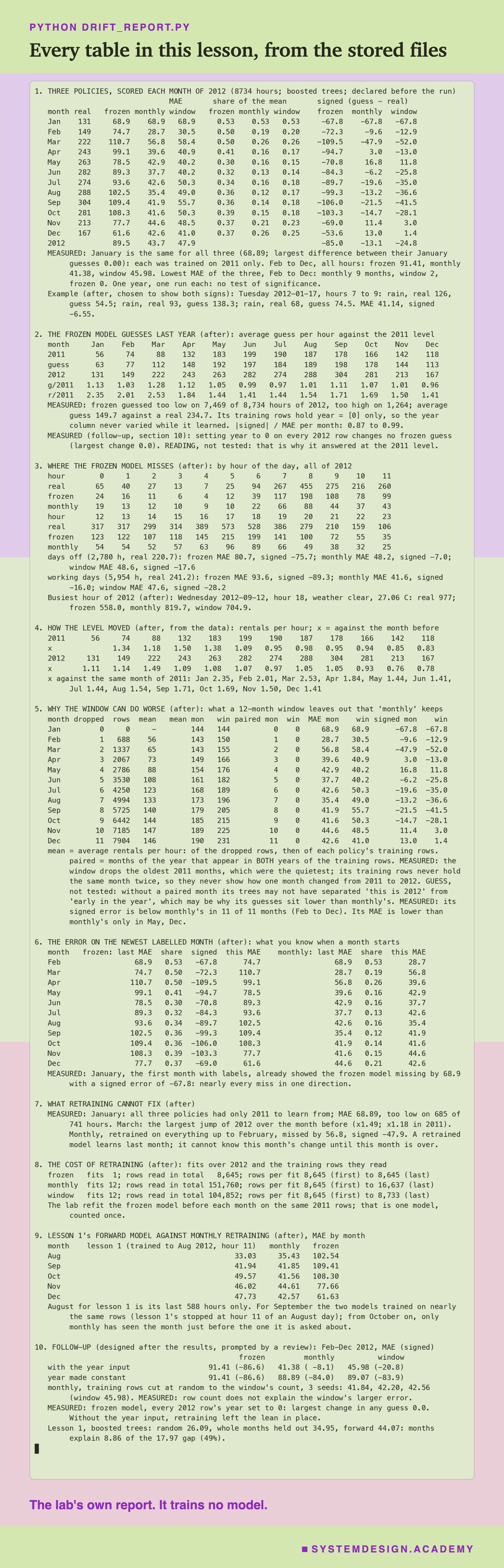
The report lives in scripts/labs/prodbreaks/drift_report.py. It reads the lab's stored results, results/drift.json, the Bike Sharing data itself from scikit-learn's local copy (for the month, hour and working-day columns of each row), and lesson 1's stored report, results/sp-report.json, for the comparison on the last slide. It trains no model. A json mode writes the numbers to results/td-report.json, which the figures read, and the figure script checks them against drift.json again before it draws anything.

Before it prints anything, it checks the files against each other. The stored real counts must be the counts in the data, hour for hour. Every month's MAE and signed error are computed again from the stored guesses and must match the stored scores. The number of training rows stored for each month must match the policy's rule applied to the data. If anything differs, the report stops. Every explanation it prints starts with MEASURED or GUESS, so that a reader of the report can tell a count from my reading of it.

This box has no model in it. It holds all 8,734 hours of 2012 in time order: the month, the hour of the day, whether it was a working day, the real count, and the guess of each of the three policies, rounded to whole bikes. It runs in your browser.

As it is, the box prints the error over all of 2012 for each policy (frozen 89.5, monthly 43.7, window 47.9) and then the table by month. Because the guesses are rounded to whole bikes, a few monthly numbers differ from the lesson by one in the last decimal (the largest difference is 0.03); the report's box mode checks every one.

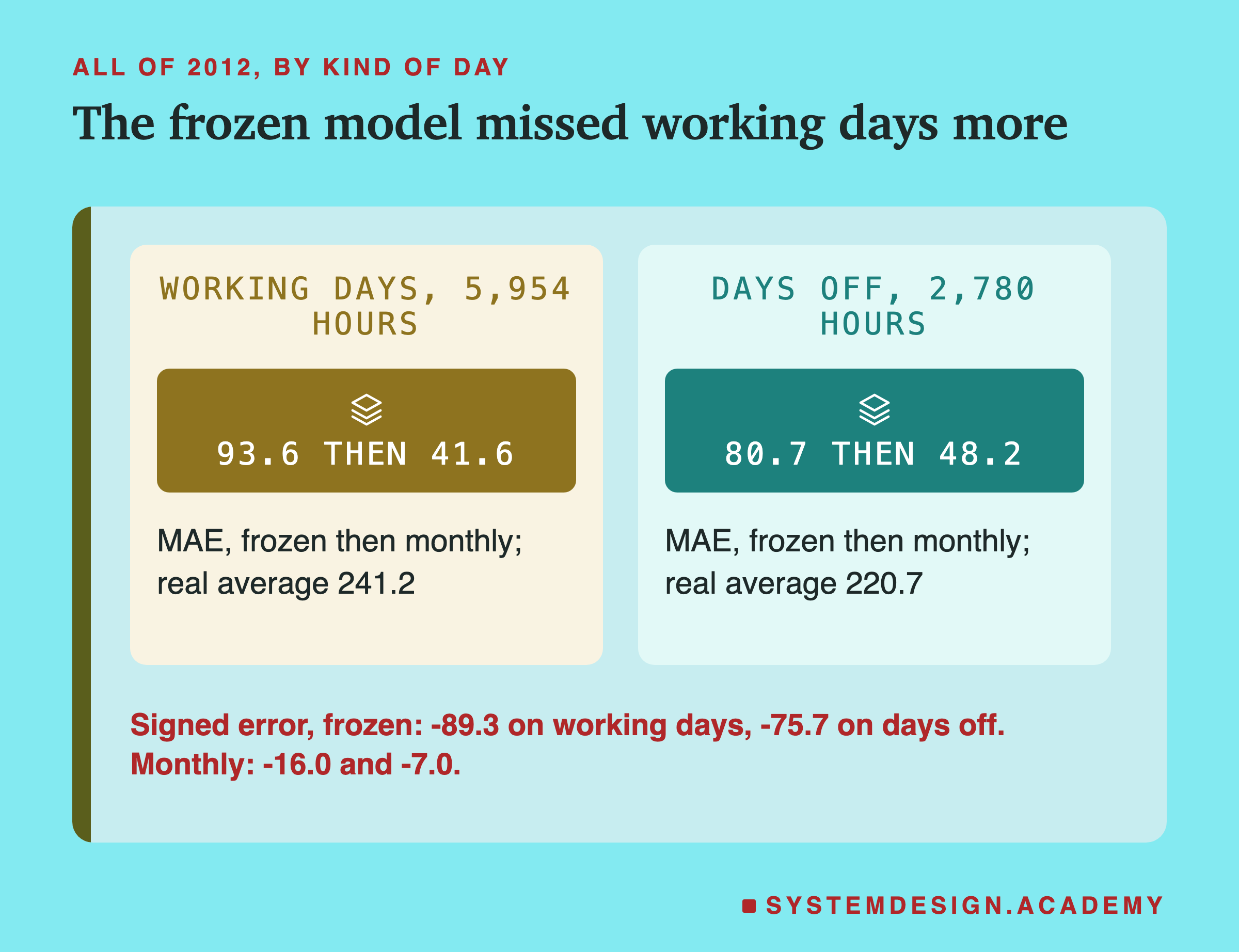
Try by_hour('frozen') and then by_hour('monthly') to see the rush-hour misses shrink and the night-time ones grow a little. Every function takes a rule for which hours to keep, so you can cut the year your own way: mae('frozen', lambda i: WORKING[i] == '1') gives the frozen model's working-day error; signed('window', lambda i: MONTH[i] in (6, 7, 8, 9, 10)) shows the window's lean from June to October; by_month(lambda i: HOUR[i] in (8, 17, 18)) gives the month table for the three peak hours only. Every number you get comes from the real guesses of the lab's models.

Loading. fetch_openml("Bike_Sharing_Demand", version=2, as_frame=True) downloads the data (or reads the local copy) as a pandas table. X is the 12 input columns and y is count, the answer. The line month = X["year"].astype(int) * 12 + X["month"].astype(int) gives every hour a month number: 1 to 12 for 2011 and 13 to 24 for 2012. This one number is what makes the policies easy to write, because "everything before July 2012" becomes month < 19.

The model. new_model builds a fresh model every time it is called, exactly as in lesson 1: a ColumnTransformer turns the four word columns into number codes with an OrdinalEncoder, passes the eight number columns through unchanged, and hands them to HistGradientBoostingRegressor(random_state=0). make_pipeline joins the steps so that the same column handling runs when the model learns and when it guesses. train(rows) fits a new model on the rows where rows is true.

The frozen policy is one line, run once, outside the loop: frozen = train(month <= 12). It learns 2011 and is never touched again.

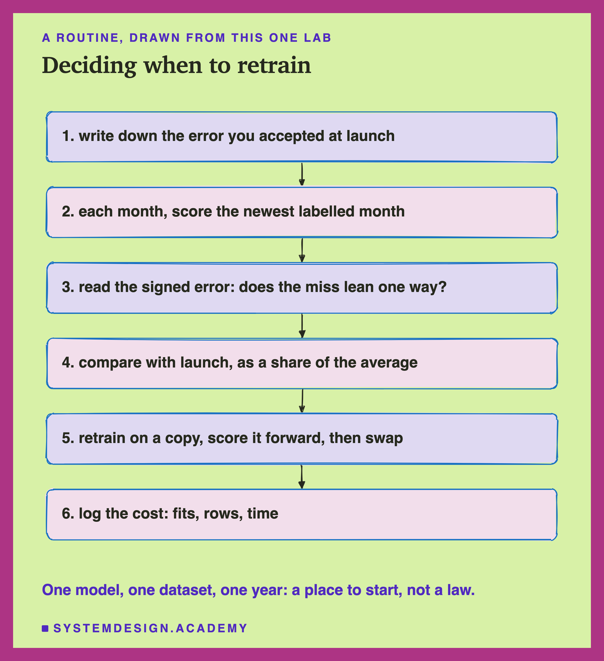
Write down the launch error. Before a model goes live, score it on a forward test, as in lesson 1, and keep that number: the MAE, the signed error, and the MAE as a share of the average. That is the line every later month is compared with. Without it, a newest-month error of 68.9 means nothing.

Score the newest labelled month, every month. As soon as a stretch of real answers arrives, score the model on it. Choose the stretch to match how fast answers arrive and how fast your world moves: a month suited this data; a week or a day might suit a busier one.

Read the sign, not only the size. A signed error close to the MAE means the misses all lean one way, which points at a change in level. Here, January's newest-month reading of 68.9 with a signed error of -67.8 said so on the first day of February.

Compare as a share. When the world gets busier, the raw error grows for that reason alone. Compare the share of the average with the share at launch, and look at the slices that matter to your users (a slice is a subset of the hours, such as every 8 in the morning, or every day off), such as the rush hours here.

Retrain on a copy, then test it before you swap. Train the new model on the chosen rows, score it forward on the most recent stretch it has not seen, compare it with the model in use, and only then replace the old one. Keep the old one ready. Check what your data rule throws away: here, a 12-month window threw away the only rows that showed one year against the next. And check that some input can express the change you expect: here that input was the year.

Log the cost. Count the fits, the rows, the time and the checks. A policy you cannot afford to run every month is not a policy.

Retrain regularly when the world keeps moving, and the model has an input that can show how. Demand that grows, prices that rise, a user base that changes. Here, ridership grew between the years, and retraining every month cut the average miss from 89.5 to 43.7. But the follow-up showed it did so through the year input. With the year made constant, monthly retraining scored 88.89 from February to December, against 91.41 for the frozen model, and it kept the lean (signed -84.0). Fresh rows alone did not fix the lean here. Before you count on retraining, ask what input lets the model tell the new world from the old one: a year, a date, a count of stores or members, a price.

Retrain when the newest labelled month leans one way. A signed error nearly as large as the MAE is the clearest signal in this lesson. It appeared in the very first month and never went away for the frozen model.

Keep all history, or a long window, when the old data still teaches something. Here, the old months were the only way for the model to compare one year with the next, and the 12-month window, which threw them away, did worse in 9 of 11 months (why is a guess). The window's larger error was not about having fewer rows: the monthly policy cut to the window's row count still scored 41.84 to 42.56.

Use a short window when the old data describes a world that is gone. A rule change, a new pricing plan, a redesign that changed how people behave. Then the old rows teach the wrong thing, and forgetting them can help. Decide by checking what the window drops, not by habit.

Do not expect retraining to see a change coming. The first month after a change (January here) and a sudden jump inside the year (March here) cannot be learned before they happen. For those you need something outside the model: someone who knows what is coming, or checks on the inputs, which the later lessons of this chapter measure.

Do not retrain blindly. If the newest month's miss is large but goes both ways, the model may be noisy rather than old, and more of the same data may not help. And a new model that nobody checks before it goes live is its own risk. Retrain on a schedule you can afford to check.

A frozen model is fine when the world really stays still. A model that sorts photos of parts on a production line that does not change, or one whose job and data are fixed by rule. Even then, keep scoring the newest labelled stretch: a frozen model is only safe while you are watching it.

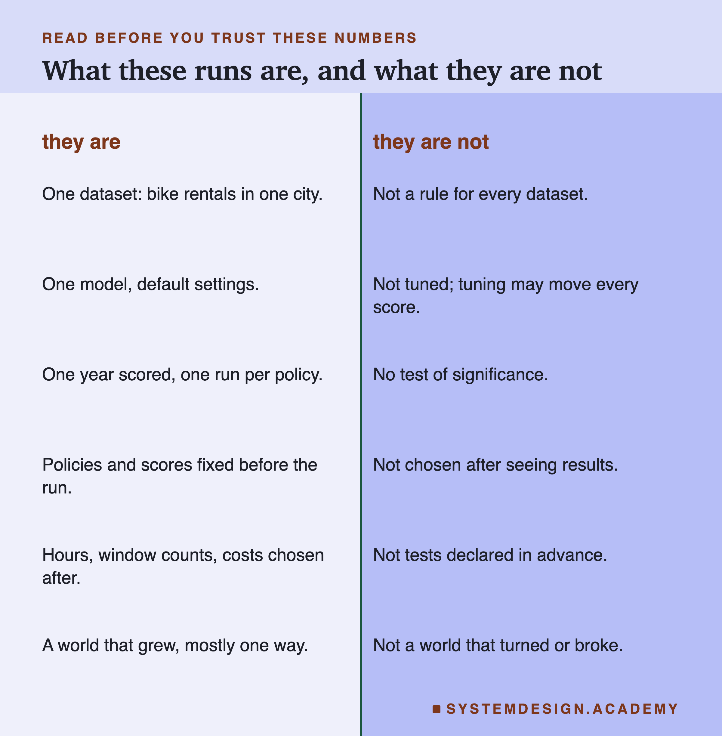
One dataset, one year. Hourly bike rentals in one city, scored over the twelve months of 2012. The drift here was mostly one kind: the level rose. In data where the world turns around, breaks suddenly, or changes shape rather than size, the three policies could rank differently. I make no claim that monthly retraining halves the error anywhere else.

One model, default settings, one run per policy. The boosted trees use a fixed seed, so a rerun gives the same numbers, which the student script confirmed for four months. But there is one run per policy on one year, and the design declared no test of significance. The gap between frozen and the other two is large and holds in every month after January. The gap between monthly and the window is smaller and goes the other way in two months, so I call it what happened here, not a finding. The follow-up is also one run per setting (three seeds for the cut rows), on the same year.

Not tuned. A tuned model might do better under every policy. Nothing here says whether tuning would change the order.

The design was declared; the reading was not. The policies, the months and the four stored numbers were written in drift_lab.py before the run. The tables by hour and by kind of day, the comparison with 2011, the window's dropped months and paired months, the newest-month reading, the cost counts, the example day, the busiest hour and the comparison with lesson 1 were all chosen after I saw the results. The follow-up run (no year input, cut rows, year set to 0) was designed after the results too, prompted by a review of this lesson, and its design is written in drift_lab.py under followup. Read them as a description of this run, not as tests I set out to pass.

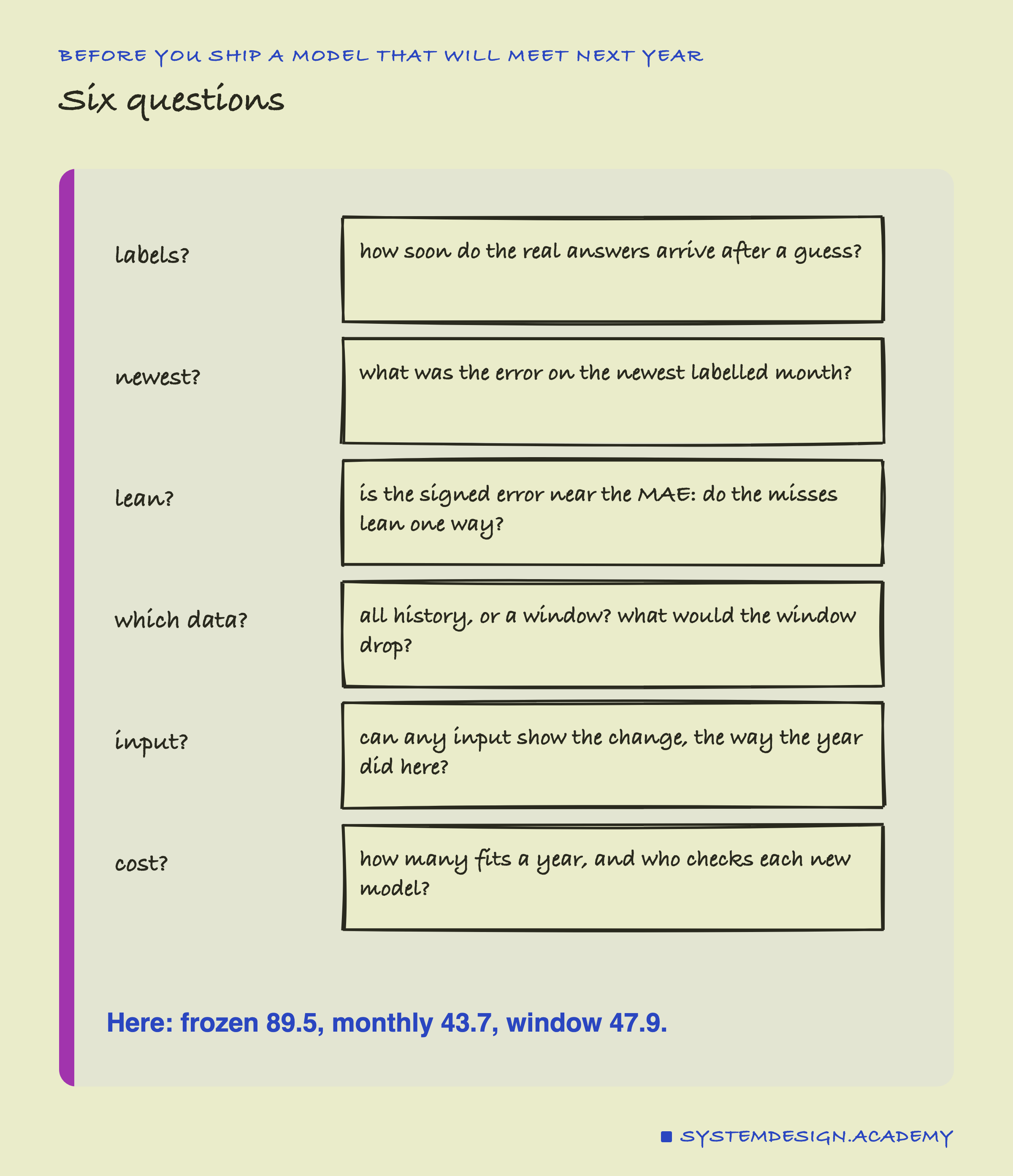
Take a model that you or your team shipped more than a few months ago. Find out when its real answers arrive, collect the most recent stretch of them, and score the model on it: the MAE, the signed error, and the MAE as a share of the average. Put those next to the scores from before launch. If the signed error is nearly as large as the MAE, the model is behind the world, and you now know which way.

Then write the policy down. How often will you retrain, on which rows, and who checks each new model before it replaces the old one? If you choose a window, list what it throws away. It takes an afternoon, and it turns "we should retrain sometime" into a rule you can follow and a number you can watch.

This lesson measured drift after the answers arrived: each month's error was known only once the month was over. That leaves a gap: in January 2012, nothing in the model's error could warn anyone until February. The later lessons of this chapter look at what else can go wrong between training and serving, and at watching the inputs themselves, which can move before any answer arrives.