Let me start with a newspaper.

An editor has a story that is too long for its page. Every paragraph takes space, and space costs money. So she cuts. She does not cut at random. She reads the story, finds the paragraph whose loss hurts the story least, cuts it, and reads again. Then she repeats, until the story fits.

Now imagine two paragraphs that say almost the same thing. If she asks "can I lose this one?", the answer is yes, because the other one still tells the reader. If she asks the same about the second one, the answer is also yes, for the same reason. Each paragraph looks useless. But if she cuts both, the story has a hole in it.

A machine learning model has the same problem with its inputs. Every input costs something to compute and to store, every day the model runs. Some inputs carry the story. Some repeat each other. In this lesson I measure which ones earn their place, on real data from a real shop.

This lesson uses the same shop, the same customers and the same question as the rest of the chapter. If any of that is new, please read what a feature is first. That lesson built six simple features from each customer's history, such as how many days since their last order and how much they have spent. The question is always the same: at the start of a month, will this customer buy something in the next 30 days?

The lesson on window aggregations added 15 more columns: orders, spend and products over the last 7, 30, 90, 180 and 365 days. Together with the six, the model scored a little higher. But that lesson also noted that it now had more than three times as many columns.

The lesson on categorical features at scale added a block of 842 hashed columns for each customer's favourite product, for a small gain.

So I now have a pile of features, and each one has a price. This lesson asks the question a team asks once the pile gets big: which of these features earn their compute?

Please read this slide slowly if any word is new. Every slide after it uses these words.

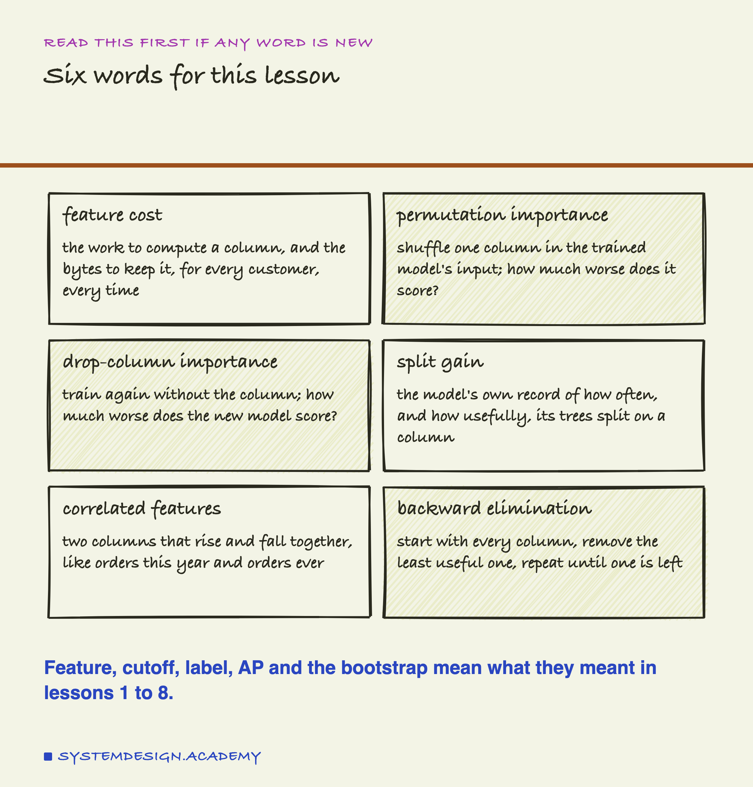
Feature cost is what a feature takes to exist. It is the computer work to calculate it, and the bytes to store it, for every customer, every time the features are refreshed. Think of the space a paragraph takes on the page.

Importance is how much the model's score depends on one feature. There are several ways to measure it, and this lesson uses three.

Permutation importance shuffles one column. Think of mixing up one paragraph's sentences with other stories' sentences, and seeing how much worse the article reads. In a table, it means giving every customer another customer's value for that one column, and scoring the same trained model again. I also call it shuffle importance, because that is what it does.

Drop-column importance removes the column completely and trains a brand new model without it. It is the editor actually cutting the paragraph and reading again. In this lesson, drop importance is AP lost, so a minus sign means the model scored higher without the column.

Split gain is a record the model keeps about itself. Each tree splits on columns, and each split improves the training score by some amount, its gain.

Two features are correlated when they rise and fall together. Backward elimination is the editor's method: start with everything, remove the least useful piece, repeat.

"How much does this column matter?" sounds like one question. In practice there are three common ways to answer it, and they do not measure the same thing.

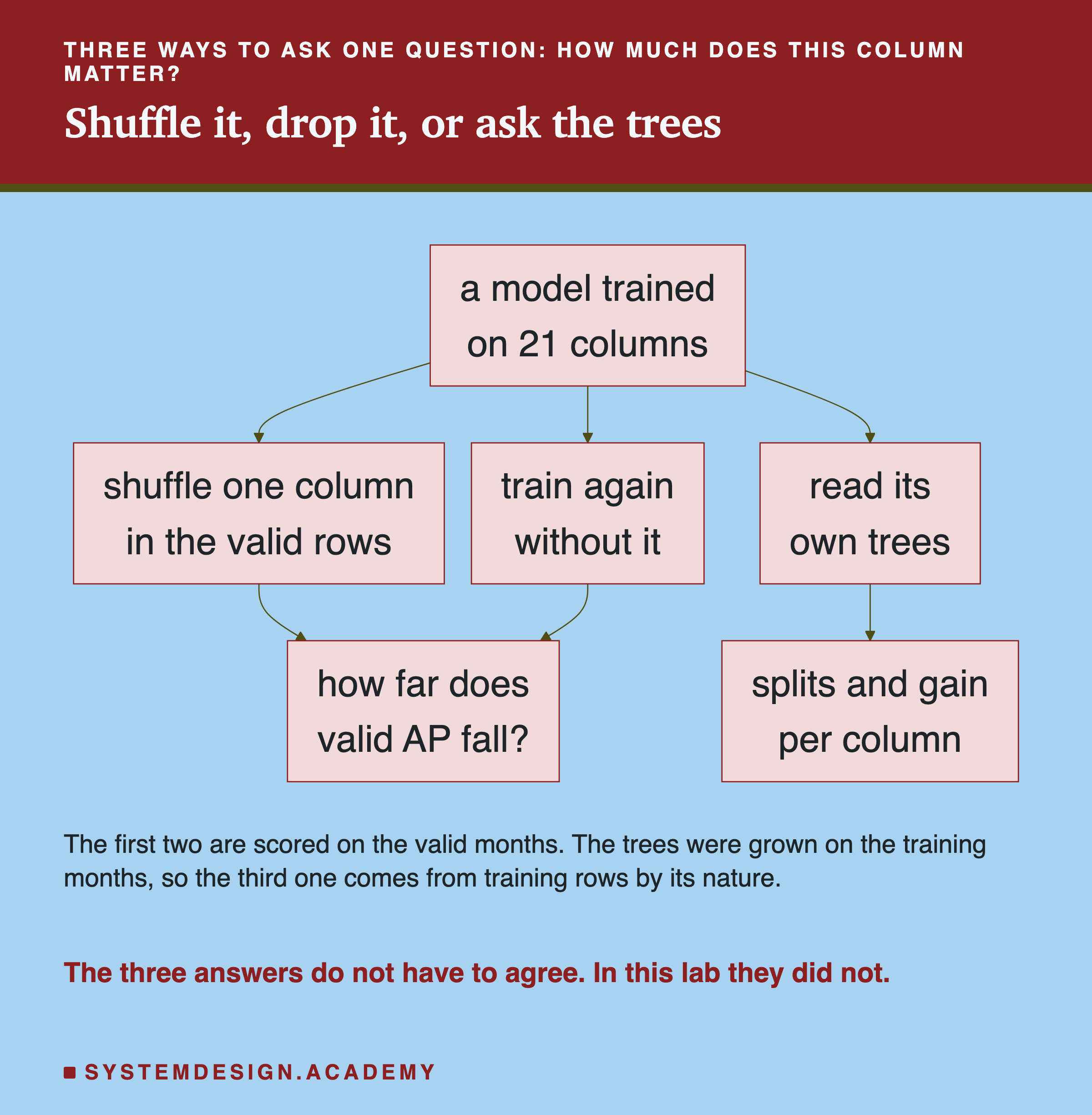
Shuffling is cheap. You train one model, then shuffle each column in turn and score again. Nothing is retrained. But a shuffled row is a strange customer. It has one customer's recent orders and another customer's lifetime orders. Later slides show how strange.

Dropping is honest but expensive. You train a new model for every column you remove. The new model can learn to use other columns instead. That is exactly what you want to know when you plan to delete a feature for real.

Split gain costs nothing extra, because the model wrote it down while it trained. But it tells you what the model leaned on, not what it needed. Those are different questions, as you will see.

I score the first two on the valid months: the three months kept aside for choosing things. The test months are only scored once, at the end.

Before I measured anything, I read what the tools and one well-known paper say about correlated features. They warn about opposite things.

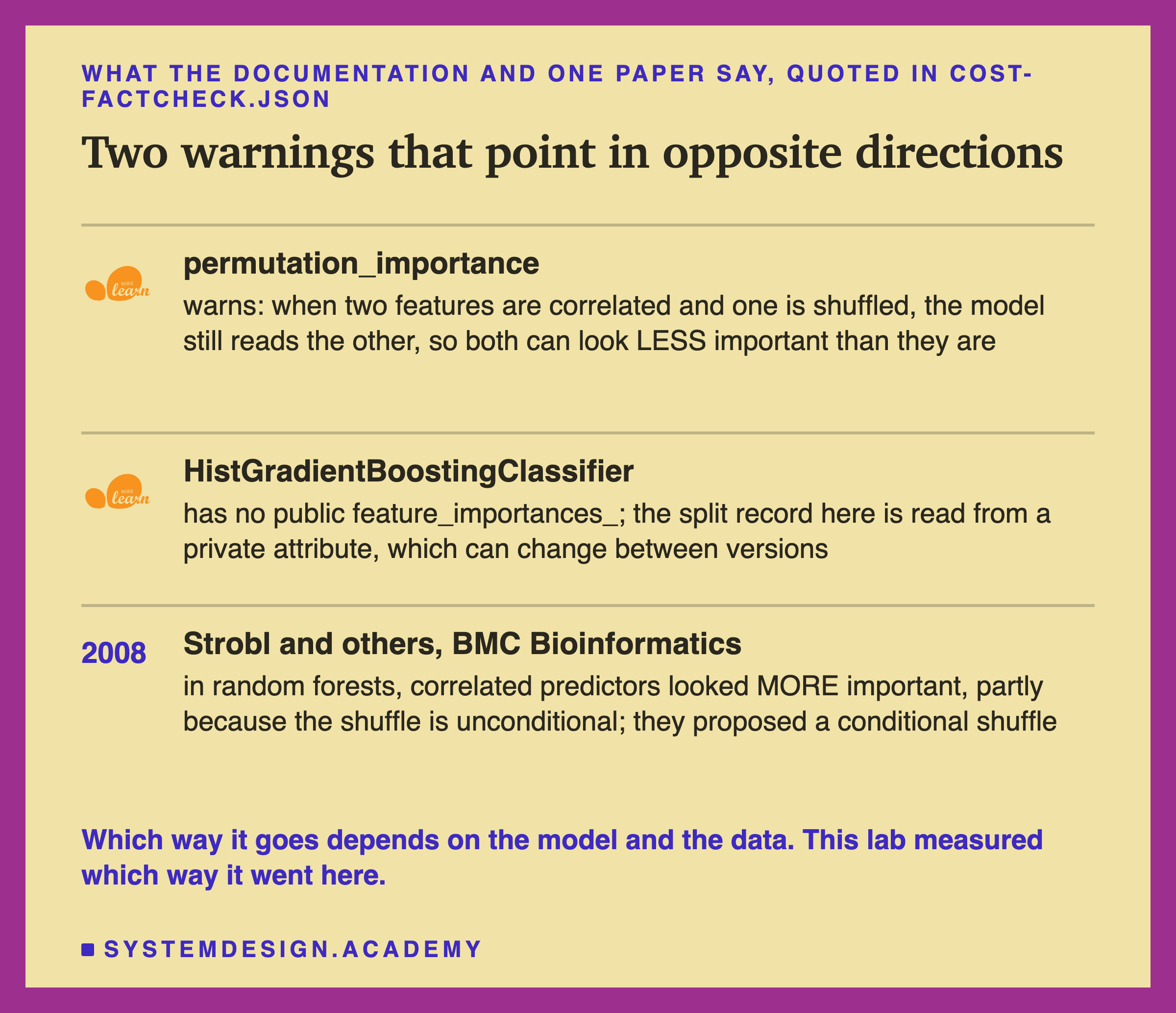
scikit-learn's permutation importance page gives this warning. In its own words: "When two features are correlated and one of the features is permuted, the model still has access to the latter through its correlated feature. This results in a lower reported importance value for both features, though they might actually be important." In plain words: each twin hides the other.

A 2008 paper by Strobl, Boulesteix, Kneib, Augustin and Zeileis in BMC Bioinformatics looked at random forests and found the opposite direction. Their abstract says the importance measures "show a bias towards correlated predictor variables", partly from "the unconditional permutation scheme". They proposed shuffling a column only among rows that are similar in the other columns, which they call a conditional permutation. I read the abstract only, so I quote nothing else from the paper.

HistGradientBoostingClassifier, the model of this chapter, lists no feature_importances_ attribute in its documentation. So I read the split record from the fitted trees through a private attribute, _predictors. Private means it can change in a future version without warning. Every quote is stored in results/cost-factcheck.json.

Here is everything the model can choose from.

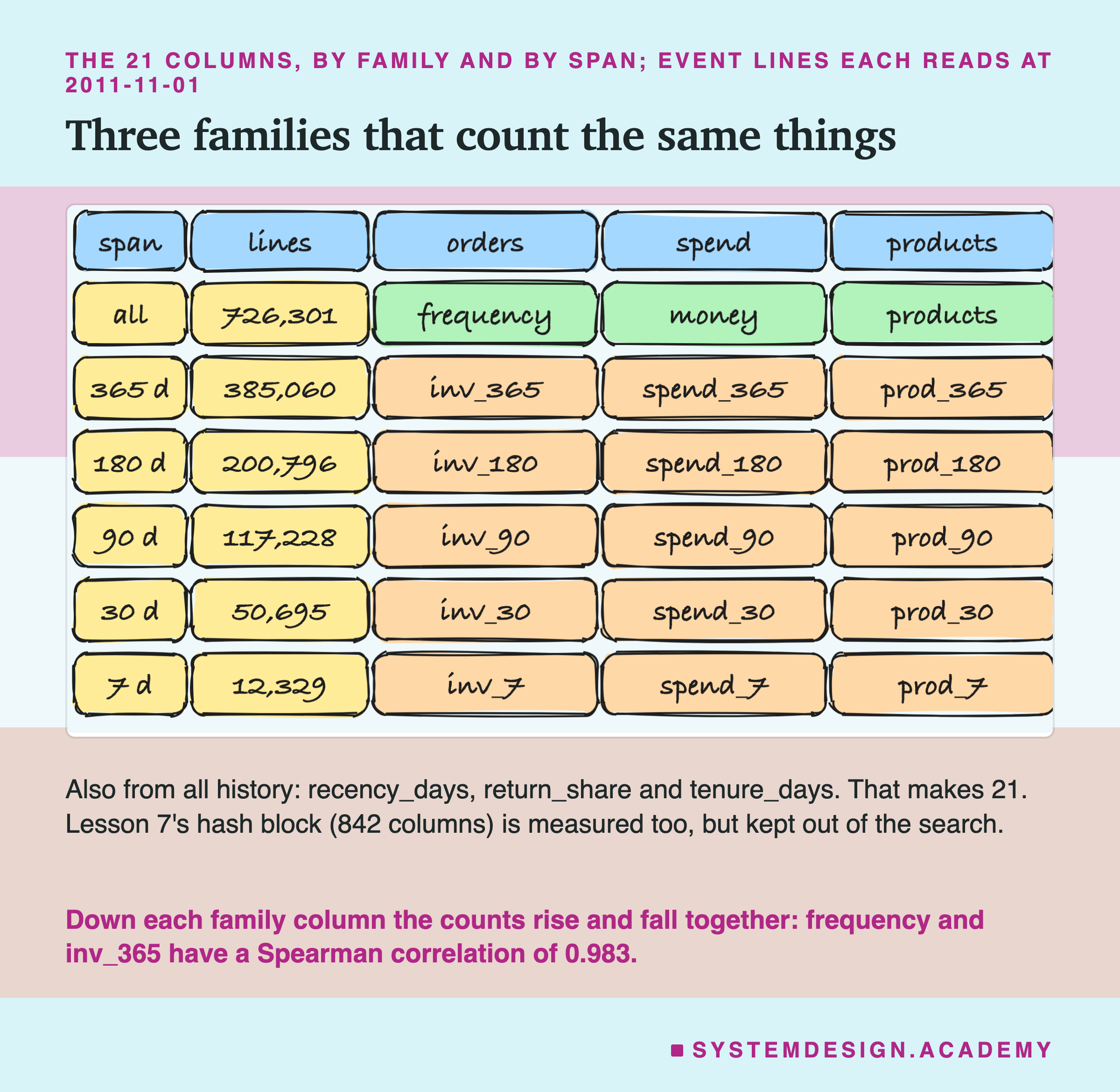
Read the table down a column and you see a family. The "orders" family has frequency, all orders ever, and five window versions, inv_7 to inv_365, the purchase invoices in the last 7 to 365 days. The "spend" and "products" families work the same way. These are twins by design: orders in the last year and orders ever are nearly the same number for most customers. Their Spearman correlation, a score from -1 to 1 for how well two columns keep the same order, is 0.983 for frequency and inv_365. For money and spend_365 it is 0.987, and for products and prod_365 it is 0.985.

The other three of lesson 1's six are recency_days, days since the last order, and return_share, the share of lines that were returns. The last is tenure_days, days since the first order.

The hash block from lesson 7 is different. It has 842 columns, 40 times as many as the other 21 together, and every model fit must sort and scan each of them. The search below needs 230 fits for each of 20 seeds, so with the block inside it the search would have taken many times longer. I decided, before the run, to measure the block separately and keep it out of the search. The lesson says so wherever it matters.

To price a feature, I wanted to time it. I could not, honestly.

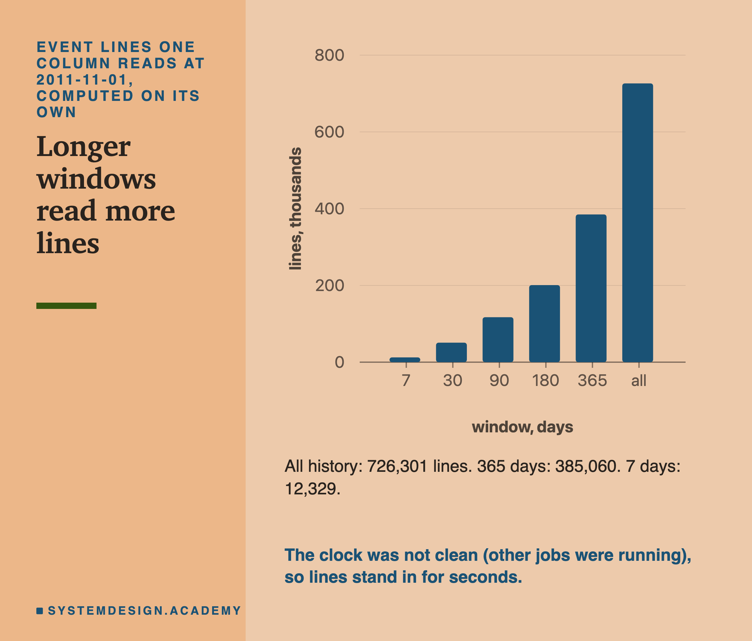
The lab has a timing mode that clocks every column for one cutoff, and it records how busy the machine was. The load average is a number for how many programs are waiting for the processor. My rule, set before the run, was to call a timing clean only if it stayed under 2. When I ran it, other lessons were being built on the same laptop and the load went from 4.44 to 3.98. So I report no seconds at all.

Instead I count lines read: how many invoice lines a column must look at to be computed, at the cutoff 1 November 2011. A column over all history reads every one of the 726,301 lines before that date. A 365-day window reads 385,060. A 7-day window reads only 12,329. That count does not depend on how busy the machine is, and the report recounts it.

Storage is simpler. Every column is one 8-byte number per customer. So 21 columns are 168 bytes per customer, and lesson 1's six are 48. The hash block, stored as a full row, is 842 times 8, or 6,736 bytes. Stored in a sparse format that keeps only the non-zero cells, lesson 7 measured about 28 bytes per row.

A subset's cost, in this lesson, is the sum of its columns' lines. That assumes each feature is computed by its own job, the way many feature stores run one job per feature definition. A team that computes everything in one pass would see different numbers.

I wrote the lab's design into the docstring of scripts/labs/features/feature_cost.py before it first ran. That includes every rule below and six guesses about the results.

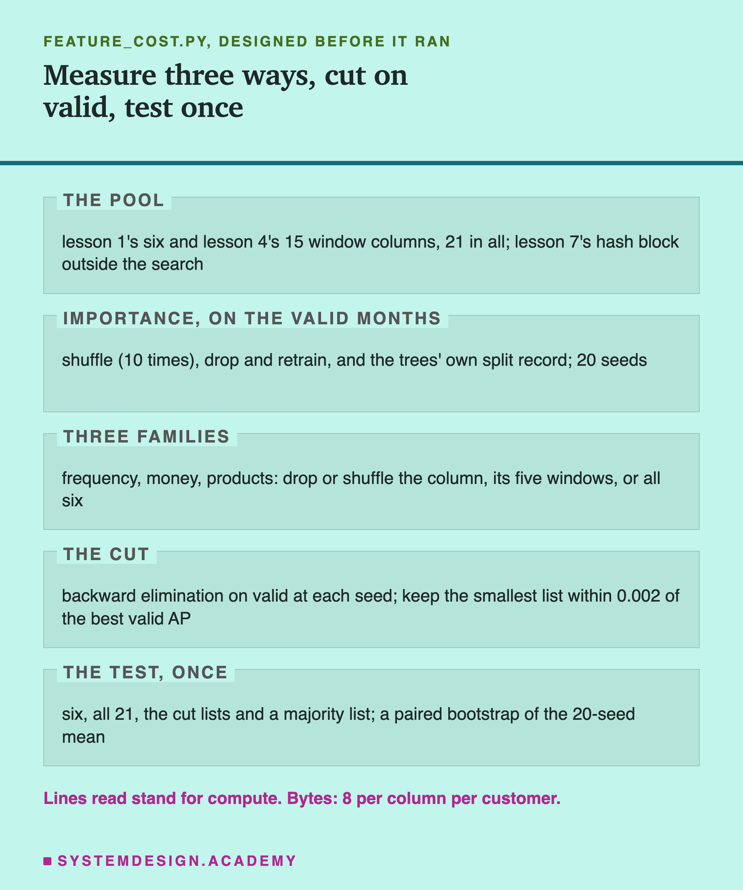
Importance. For each of 20 seeds, I trained the model on all 21 columns. I shuffled each column 10 times on the valid rows and averaged the loss. I trained a new model without each column. And I read the split counts and gains from the trees.

Families. For frequency, money and products, I dropped and shuffled three things: the single column, its five window twins together, and all six together. A group is shuffled with one row order for all its columns, so the group stays consistent inside itself.

The cut. At each seed separately, I ran backward elimination on the valid months: remove the column whose removal leaves the highest valid score, and repeat down to one column. Then I kept the smallest list whose valid score was within 0.002 of the best score anywhere on that path. I call these the cut lists. I also kept the list with the very best valid score, and a majority list: the columns that at least 11 of the 20 cut lists kept.

The test, once. Only after all of that did I score the test months, for six named sets of columns, 20 seeds each. The headline for each set is the mean over the 20 seeds.

This is a real recording of the report script, cost_report.py, in its fast mode, on the laptop where the lab ran.

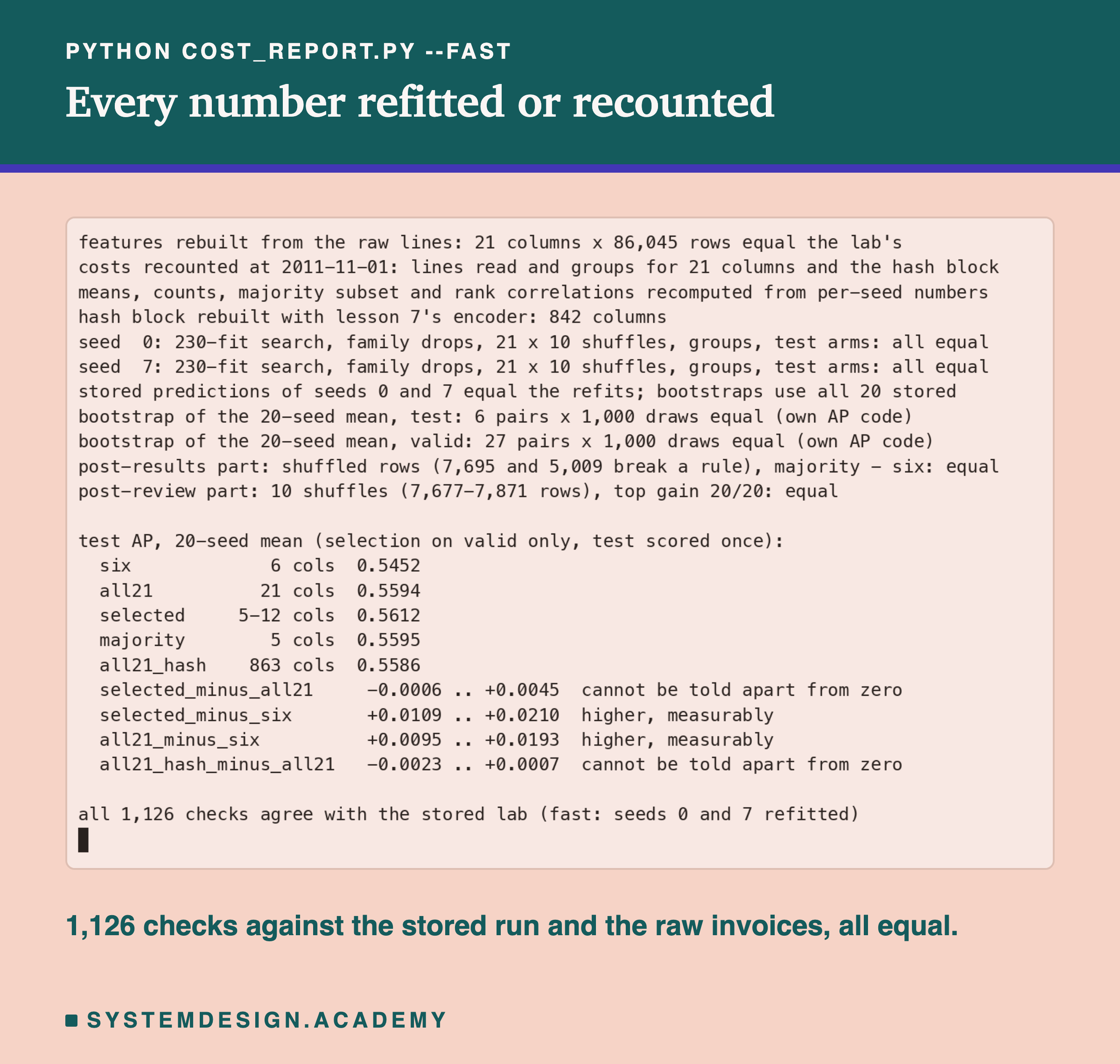
The report does not trust the lab's code for the parts that matter. It rebuilds all 21 columns from the raw invoice lines with its own grouping code and requires them to match. It recounts every column's lines. It refits seeds 0 and 7 completely, all 230 models of each search, and requires every stored number to come back exactly. Then it reruns both bootstraps with its own code for AP, and every one of the 1,000 draws must match.

The fast mode refits two seeds and checks the other 18 through their stored predictions. The full mode refits all 20 seeds and reruns both bootstraps on its own predictions. I ran it too, before the post-review checks existed, and all 6,328 of its checks agreed.

One honest note. The first time I ran the report, it stopped on a mismatch. The bug was in the report, not the lab. When a redrawn month happened to give the top-scored customers zero weight, my own AP code divided zero by zero. AP is built from precision, which means the share of the customers ranked so far who really bought. scikit-learn counts a precision with no customers yet as 0. I fixed the report, made it check its AP against scikit-learn on three draws instead of one, and it passed.

Here is the main result, on the test months, which chose nothing.

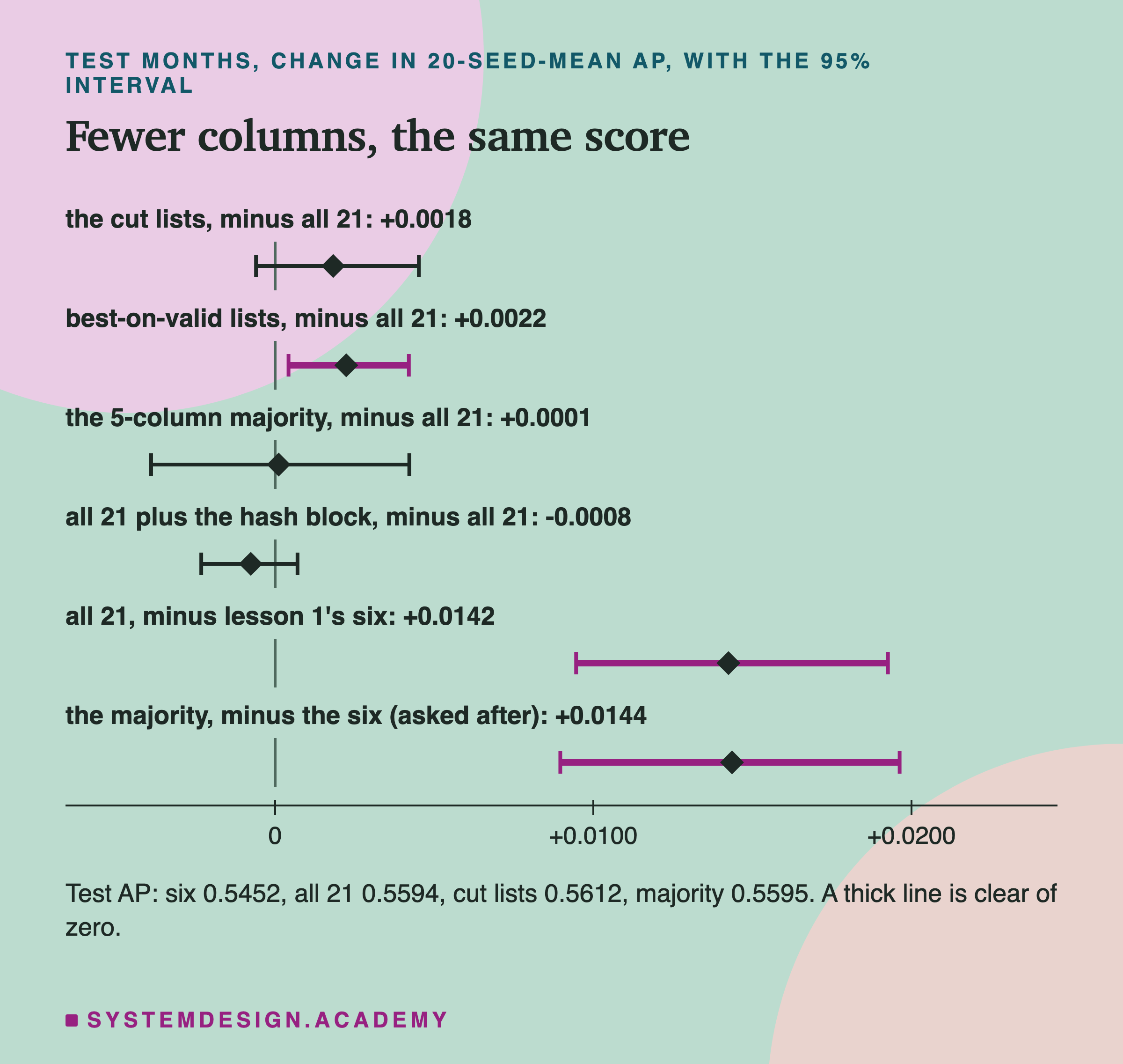
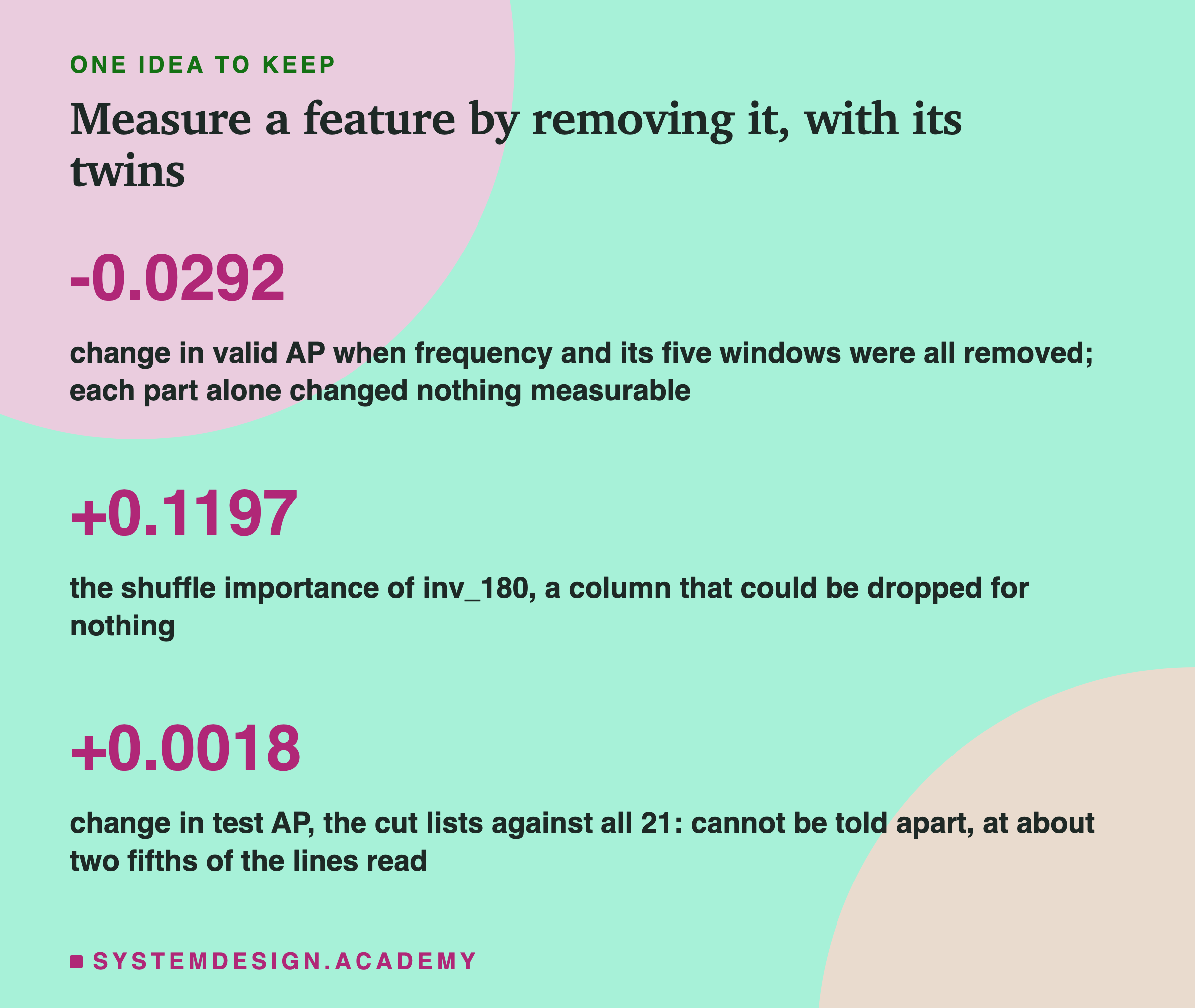
The cut lists scored 0.5612 against 0.5594 for all 21 columns, a gap of +0.0018 that cannot be told apart from zero. Its 95% interval runs from -0.0006 to +0.0045. The cut lists held 5 to 12 columns, depending on the seed. They were above all 21 in 17 of the 20 seeds and in 4 of the 5 test months. But the interval still crosses zero, so I do not call it a gain.

Both were clearly above lesson 1's six. All 21 beat the six by +0.0142, interval +0.0095 to +0.0193. The cut lists beat the six by +0.0161, interval +0.0109 to +0.0210.

The majority list, five columns, scored 0.5595, just +0.0001 above all 21, interval -0.0039 to +0.0042. The five are recency_days, products, inv_90, inv_365 and spend_365. After seeing the results, I also compared it with the six, which I had not planned. It was +0.0144 above them, interval +0.0090 to +0.0196. That is a post-results question, and the lab labels it so.

The best-on-valid lists, kept as a second rule, scored +0.0022 above all 21, and that interval, +0.0004 to +0.0042, is clear of zero. They held 7 to 20 columns. I report it, but the rule I declared first was the cut list, and that one could not be told apart.

Adding the hash block to all 21 gave -0.0008, interval -0.0023 to +0.0007, which cannot be told apart from zero.

A score alone does not answer this lesson's question. The question is the score for the price.

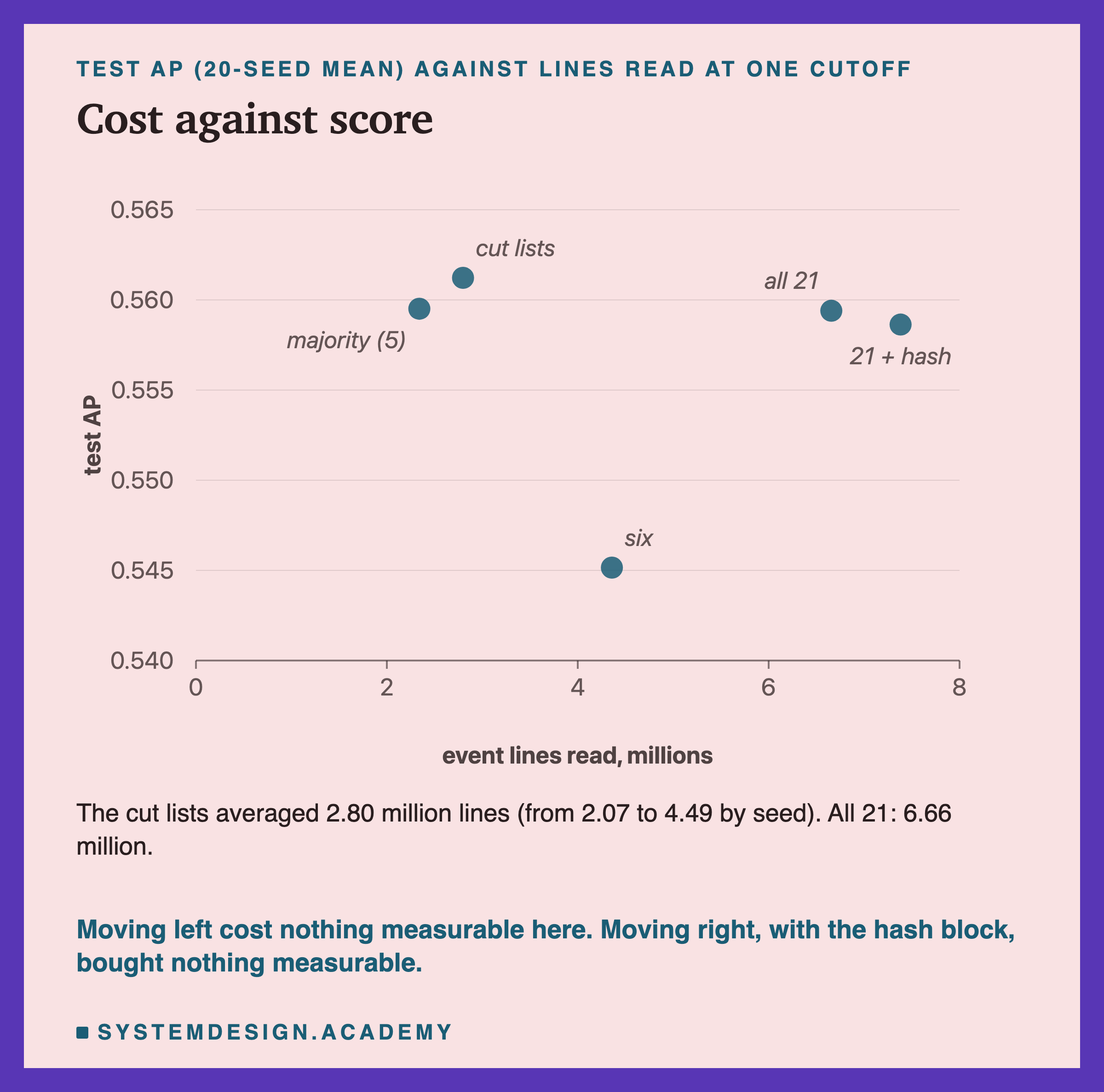
Read the chart from right to left. All 21 columns read 6.66 million lines in total at one cutoff. The cut lists read 2.80 million on average, about two fifths, and scored no lower that I could measure. The majority list read 2.34 million.

Notice where lesson 1's six sit: 4.36 million lines, and the lowest score here. Each of the six reads all history, so each one reads all 726,301 lines. The window columns are cheaper to compute in this model of cost, because they read less. That is why the cheap lists are mostly windows: of the majority's five columns, only recency_days and products read all history.

Moving right, adding the hash block, cost another 726,301 lines a cutoff and 842 columns of storage, and bought nothing measurable on test.

A frontier, in this sense, is the set of choices where you cannot get a higher score without paying more. Here the cheap lists sit on it, and the all-21 list does not. That reading is on the point estimates; the costs are exact, but the scores carry the intervals from the headline slide.

Now the main reason this lesson exists: what do the three importance measures say about each column?

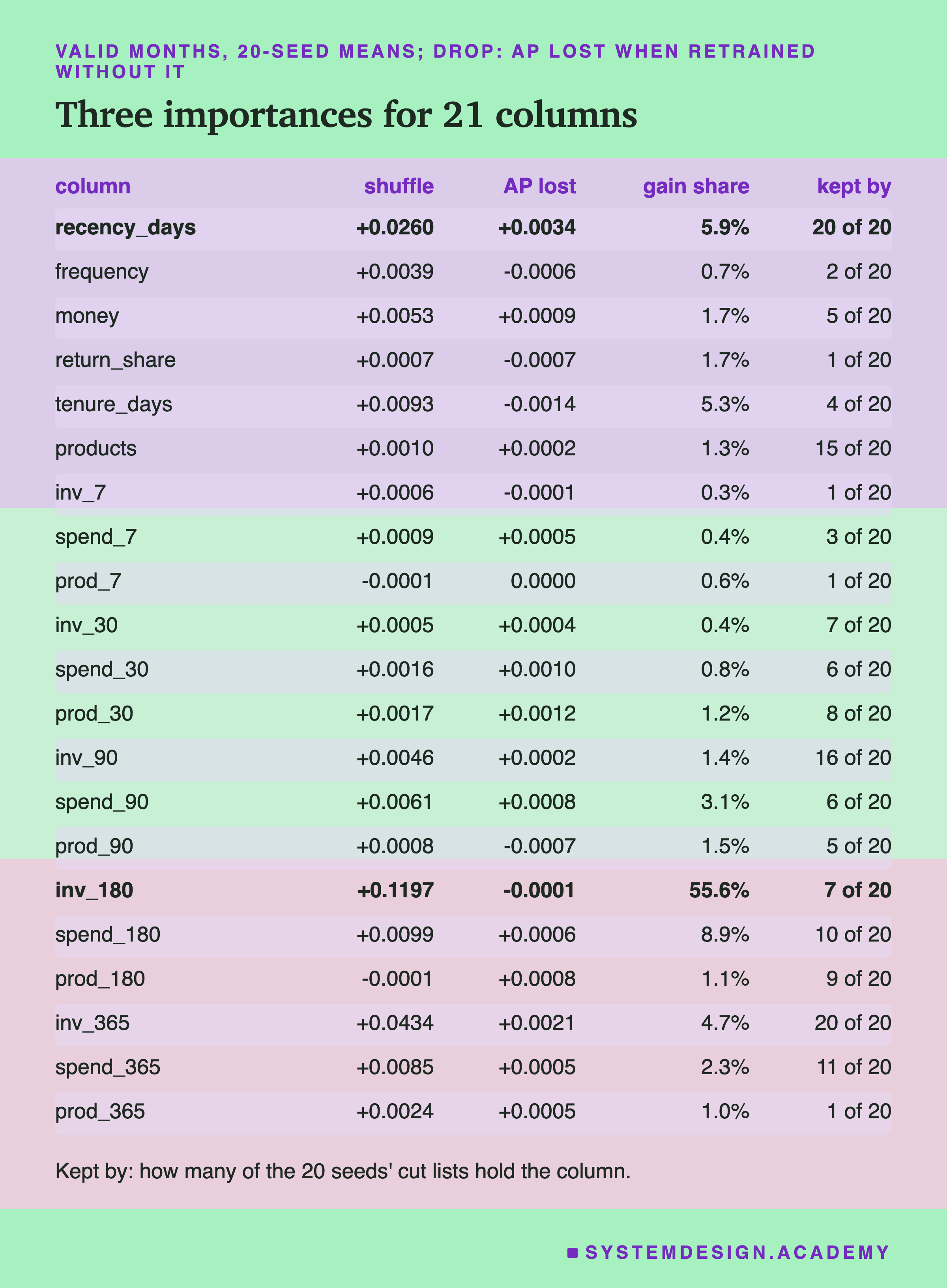
Look at the row for inv_180, orders in the last 180 days. Shuffled, it cost 0.1197 of valid AP, by far the most of any column. In the trees it took 55.6 percent of all split gain, more than half. By those two measures it is the most important feature here, by a long way.

Now look at its drop number, which is AP lost: -0.0001. The minus sign means a model trained without inv_180 scored 0.0001 higher, about the same as one trained with it. Only 7 of the 20 cut lists kept it.

recency_days goes the other way. Its shuffle importance, 0.0260, is only the third largest. Its drop importance, 0.0034 of AP lost, is the largest of all, and every one of the 20 cut lists kept it.

I measured how well the three rankings agree with a rank correlation, the Spearman score from before, applied to the lists of 21 importances. Shuffle against drop: 0.26. Split gain against drop: 0.15. Shuffle against split gain: 0.82. So shuffle and split gain largely agree with each other, and neither agrees much with the drop test.

Only five columns had a drop importance whose interval was clear of zero: recency_days, inv_365, money, and . For the other 16, removing them one at a time could not be told apart from no change.

Here is the same disagreement as a picture.

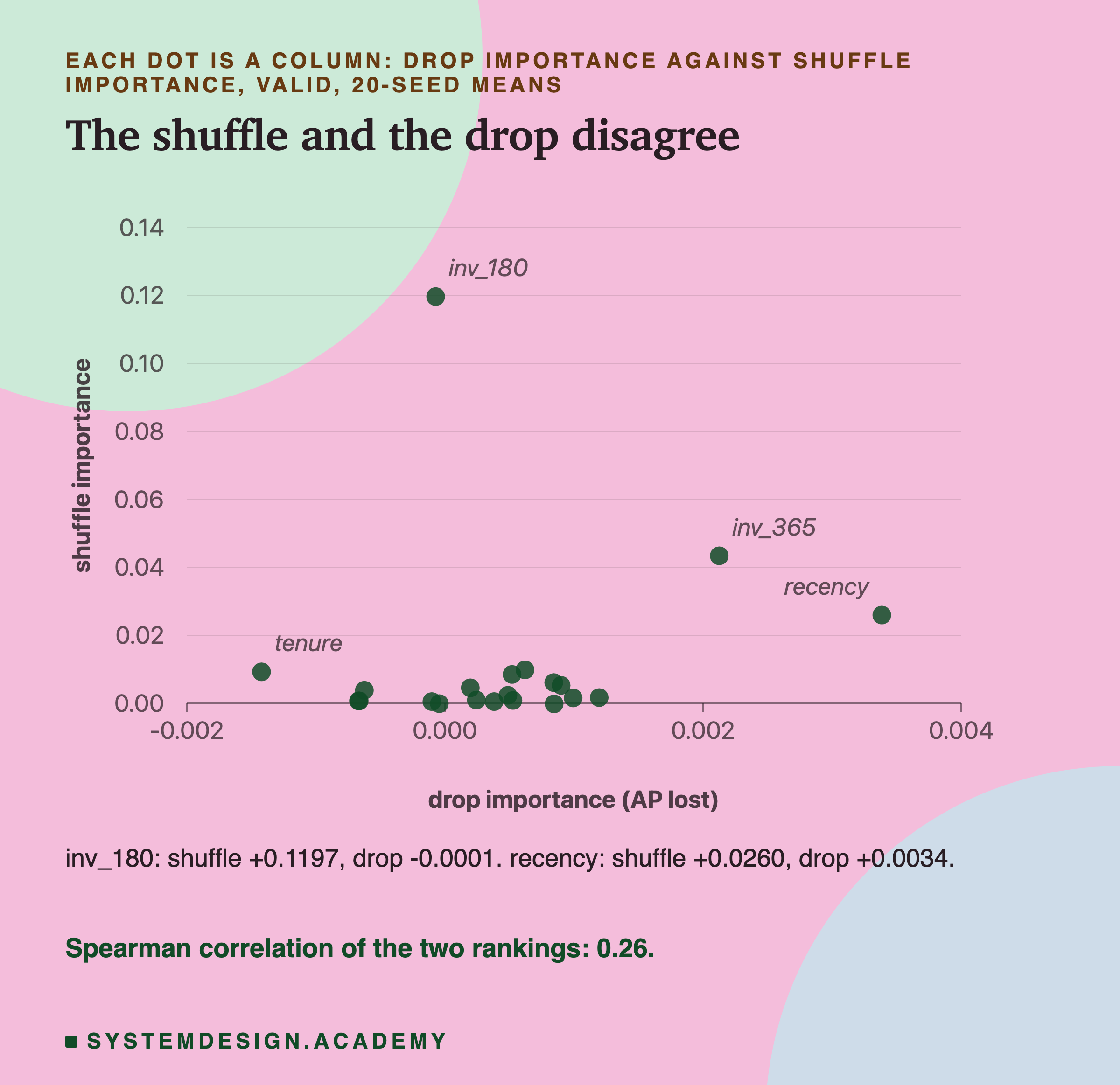
If the two measures agreed, the dots would climb from bottom left to top right. They do not. One dot, inv_180, sits high above everything at a drop importance of about zero.

So which one is right? They answer different questions, and both answers are true.

The shuffle asks: this model, as trained, how much does it rely on this column? The answer for inv_180 is: a great deal. This model put most of its early splits on it.

The drop asks: if I deleted this feature from my pipeline and retrained, would I lose anything? The answer for inv_180 is: no, because inv_365, inv_90 and frequency carry nearly the same information, and a new model simply uses them instead.

When your real decision is "should I stop computing this feature?", the second question is the one you are asking. That is why I trust the drop test more for feature cost decisions, and why it costs one new model per column.

Split gain deserves its own warning, because it is the measure that is free and therefore the one most often shown.

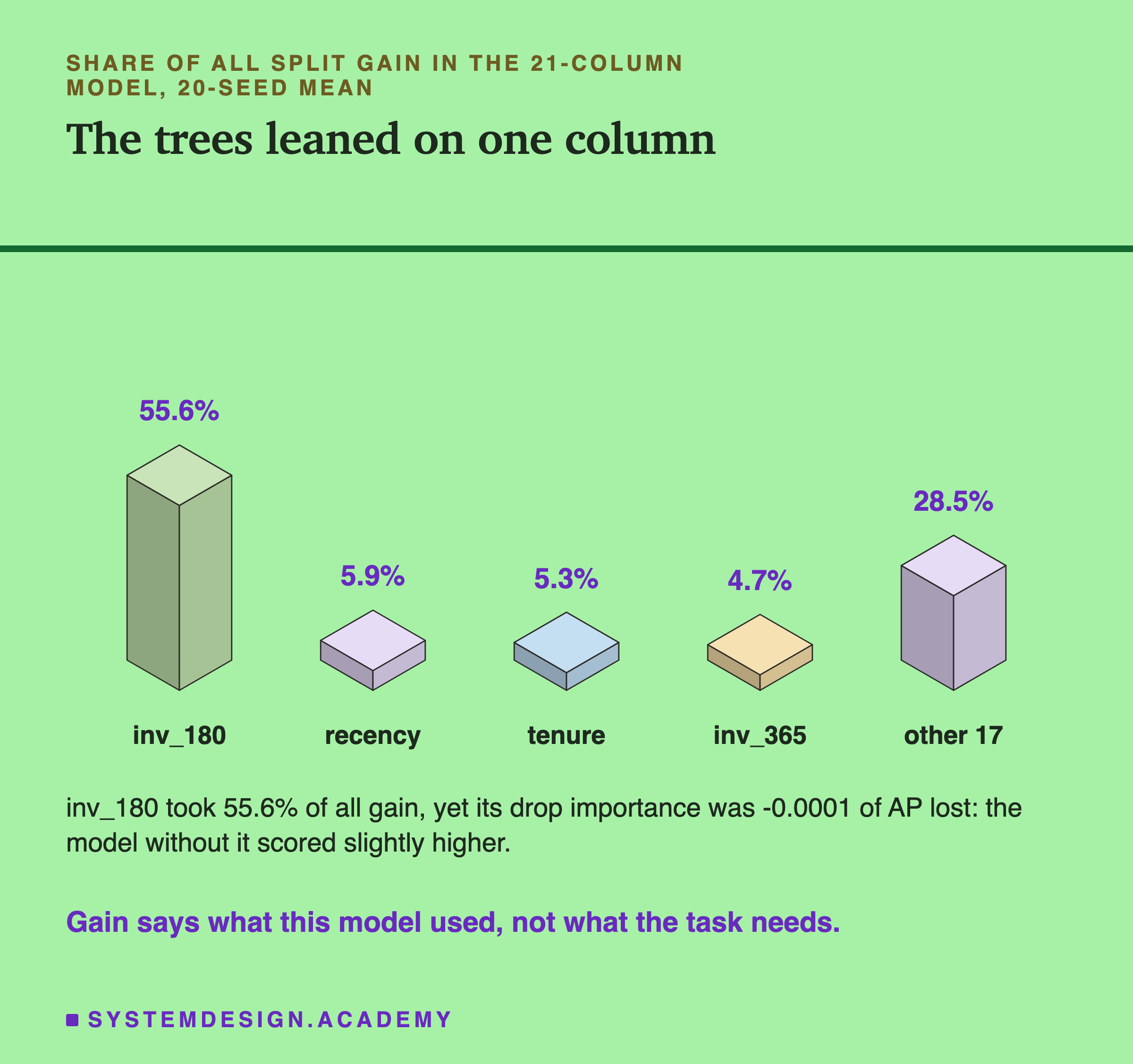
Gradient boosting builds trees one after another. The first trees fix the biggest mistakes, so their splits have the largest gains. Whichever column the first trees pick collects most of the total gain. Here that was inv_180, in the 20-seed mean.

inv_180, inv_365 and frequency all sort customers almost the same way. The first trees take whichever twin splits best by a hair. Here that was inv_180 at every seed I checked, and it then gets the credit for what the twins share. After the review, I checked all 20 seeds. inv_180 had the largest gain share at 20 of 20, from 52.7 to 58.8 percent. spend_180 was second at every seed. That check is labelled post-review in the lab.

By count of splits instead of gain, the leaders were different again: tenure_days had 14.5 percent of all splits, recency_days 13.9 percent, and inv_180 only 4.8 percent.

scikit-learn's permutation importance page makes a related point about split-based importance in general. It calls impurity-based importance "strongly biased" towards columns with many different values, and says it can rate features "that may not be predictive on unseen data". The lesson I take is simpler: split gain tells you about one fitted model, not about the feature.

Now the twins. This is the effect scikit-learn's page warns about, and the drop test shows it clearly.

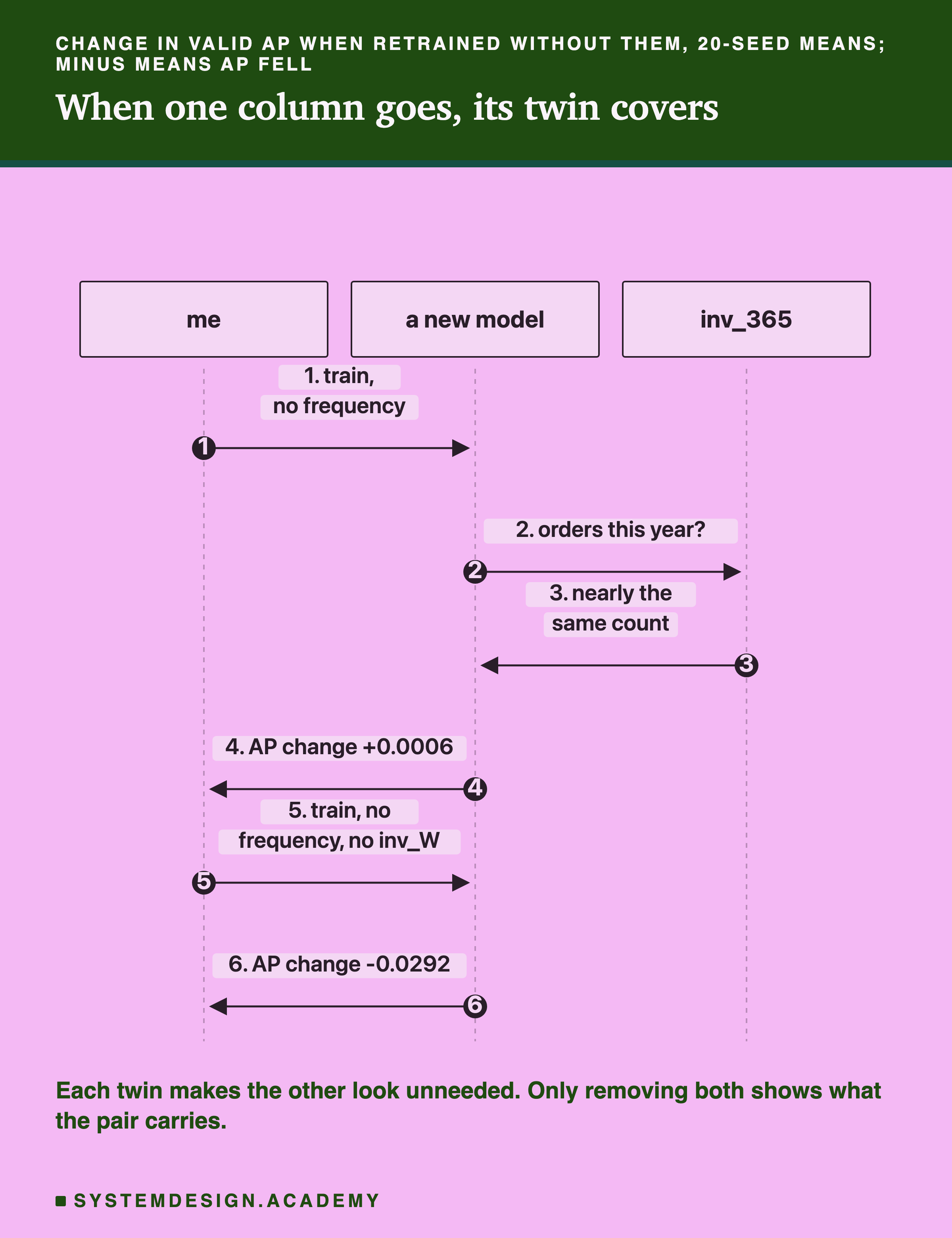
When I removed frequency and trained a new model, valid AP did not fall. On this slide and the next two I show the change in valid AP, so a plus sign means it rose. It moved by +0.0006, a tiny rise that cannot be told apart from zero. In the table's terms, that is a drop importance of -0.0006. The new model asked inv_365 instead, which gives nearly the same count.

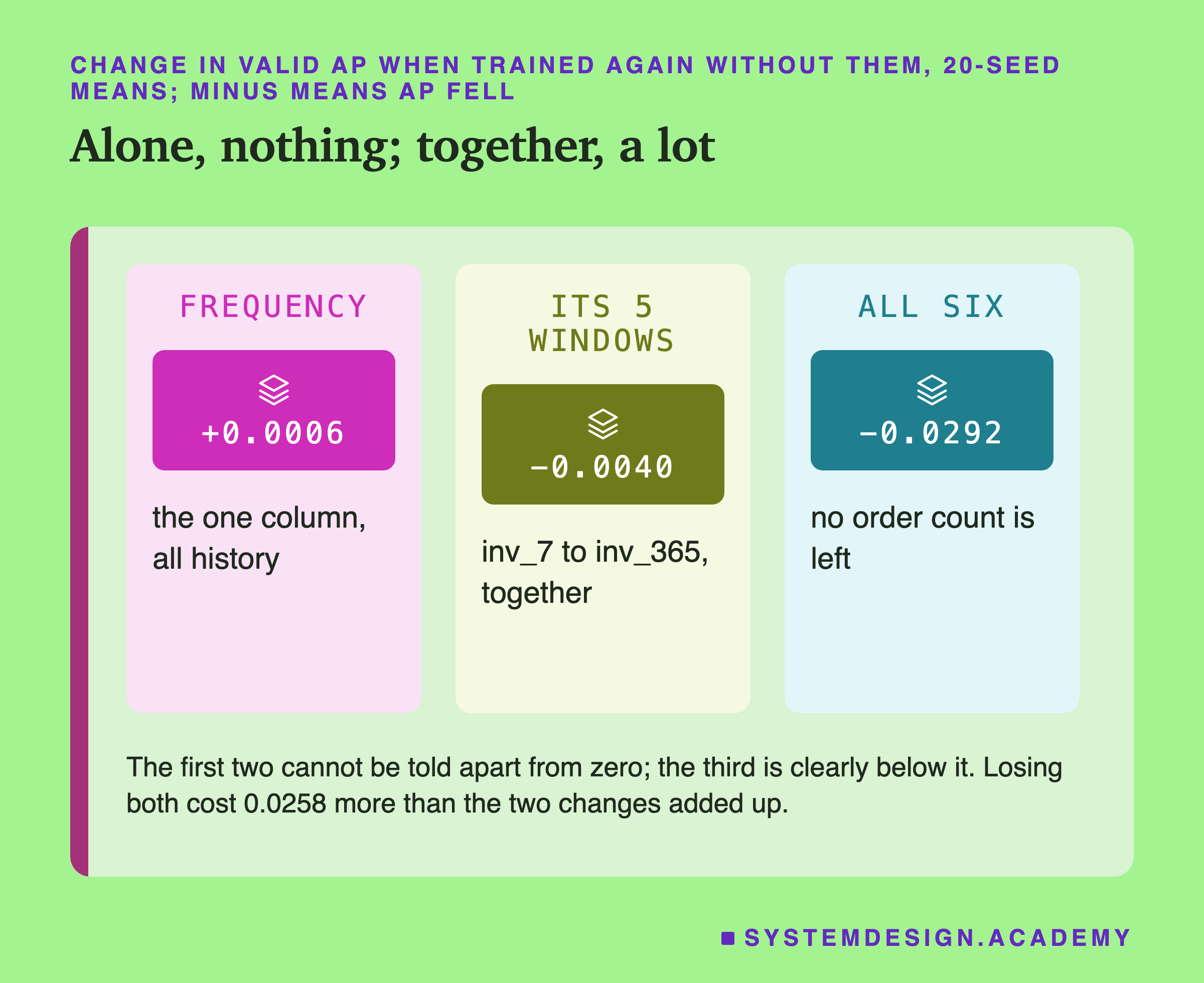
When I removed the five window columns of orders, inv_7 to inv_365, and kept frequency, valid AP moved by -0.0040. Its interval runs from -0.0081 to +0.0001, so it just crosses zero.

When I removed all six, so the model had no order count of any kind, valid AP fell by 0.0292, interval -0.0368 to -0.0209. That is clearly real, and it is more than eight times the largest single-column drop in the table, 0.0034 for recency.

The two parts, added up, predicted a change of about -0.0034. The real change was 0.0258 worse than that. I call that gap the interaction, and its interval, -0.0326 to -0.0182, is clear of zero. This is the editor's two paragraphs: each looks useless, and together they carry the story.

I expected the money family to show the same effect. It did not, and I want to show that too, because one clean example is easy to over-learn from.

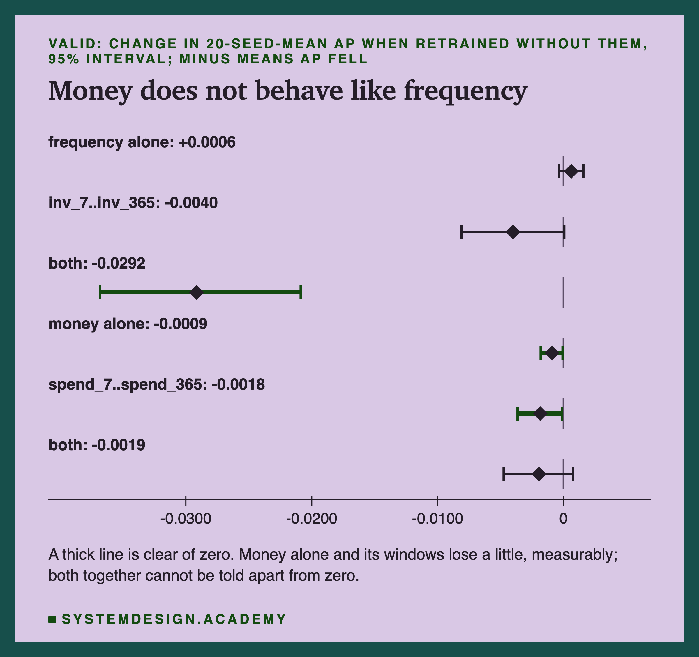
Removing money alone cost 0.0009, with an interval from -0.0018 to -0.0001. Removing its five spend windows cost 0.0018, interval -0.0036 to -0.0001. Both of those are small but measurable. Removing all six cost 0.0019, and that interval, -0.0048 to +0.0008, crosses zero. The interaction for money, -0.0016 to +0.0032, cannot be told apart from zero either.

So for money there is no hidden pair. Spend simply does not carry much that the other columns lack. One possible reason, which I did not test: the order counts and the recency already say most of what spending says about whether someone buys next month.

The products family showed nothing measurable at all: removing products alone, its five windows, or all six could not be told apart from zero.

The point is not "correlated features always hide each other". It is "they can, so test them together before you delete them".

Why did shuffling inv_180 cost 0.1197, when deleting it cost nothing? I asked this after I saw the results, and the lab labels the answer as a post-results question.

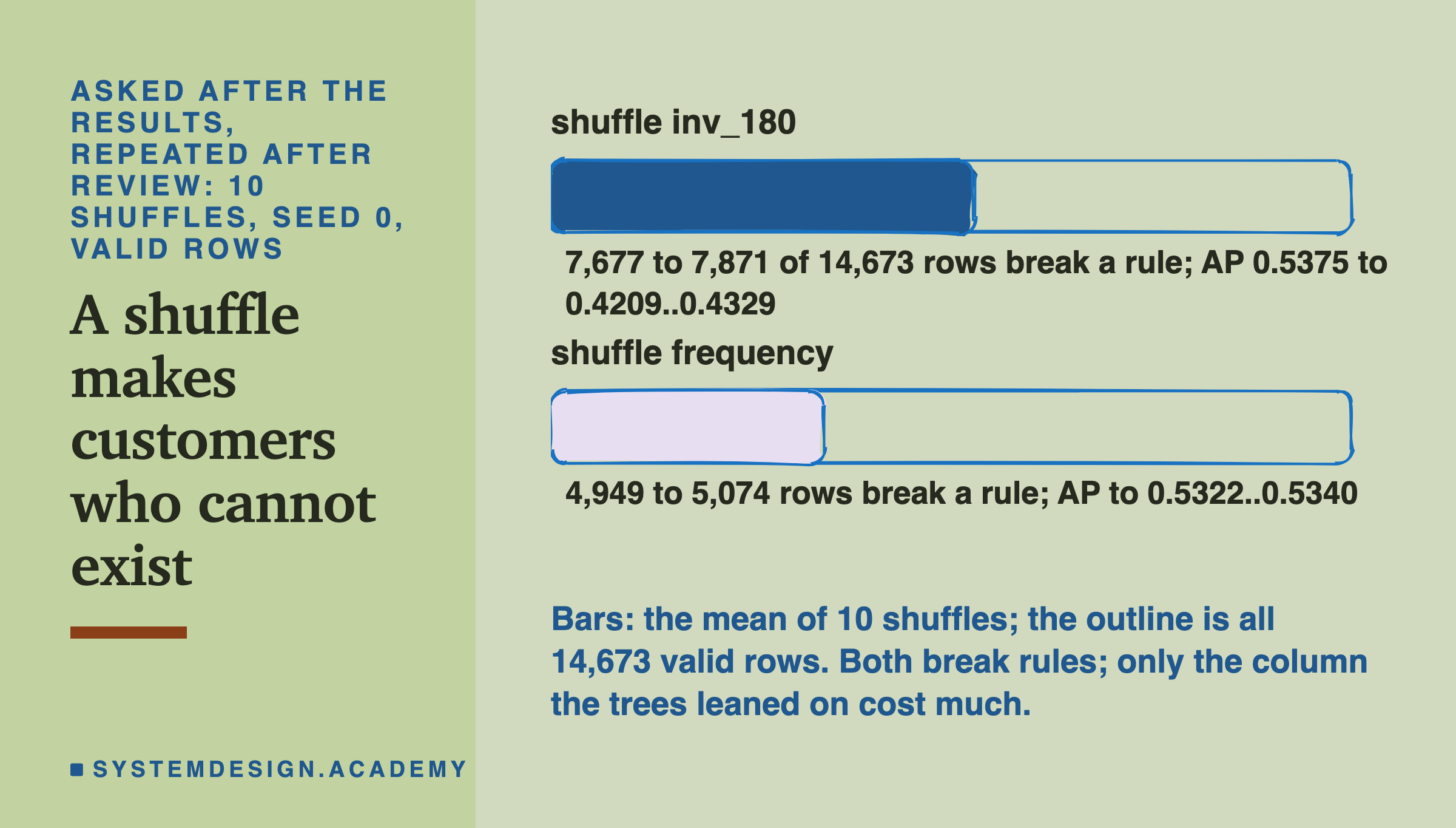
A shuffle gives each customer another customer's value for one column. That can make a customer who cannot exist. Every real row keeps some rules. Orders in the last 180 days can never be more than orders in the last 365 days. They can never be fewer than orders in the last 90 days. They can never be more than orders ever. And they must be zero if the last order was more than 180 days ago.

On the valid rows, before shuffling, no row broke any of these rules. I first counted one shuffle of inv_180, with the same random order scikit-learn uses. 7,695 of the 14,673 rows broke at least one rule, and valid AP fell from 0.5375 to 0.4268. But one shuffle is one draw, which breaks this chapter's own rule. So after the review I repeated it with 10 shuffles at seed 0, labelled post-review in the lab. Across the 10, between 7,677 and 7,871 rows broke a rule, and valid AP fell to between 0.4209 and 0.4329.

Shuffling frequency also broke a rule, frequency below orders this year, in 4,949 to 5,074 rows across the same 10 shuffles. But valid AP only fell to between 0.5322 and 0.5340. One possible reason: the model had barely used frequency.

So impossible rows alone do not explain the size of the loss. What they show is that a shuffle tests the model on customers who do not exist. I did not find where the loss lands: in the first shuffle, the rule-breaking rows held about as many top-fifth places as before, 1,840 against 1,827. Here is my reading, which fits these numbers but which I did not test. The loss comes from a model that leaned heavily on one column, fed values for it that do not fit together. This is the direction Strobl and others warned about: correlated predictors looking more important, not less.

Now lesson 7's hash block, measured outside the search, with the same three measures.

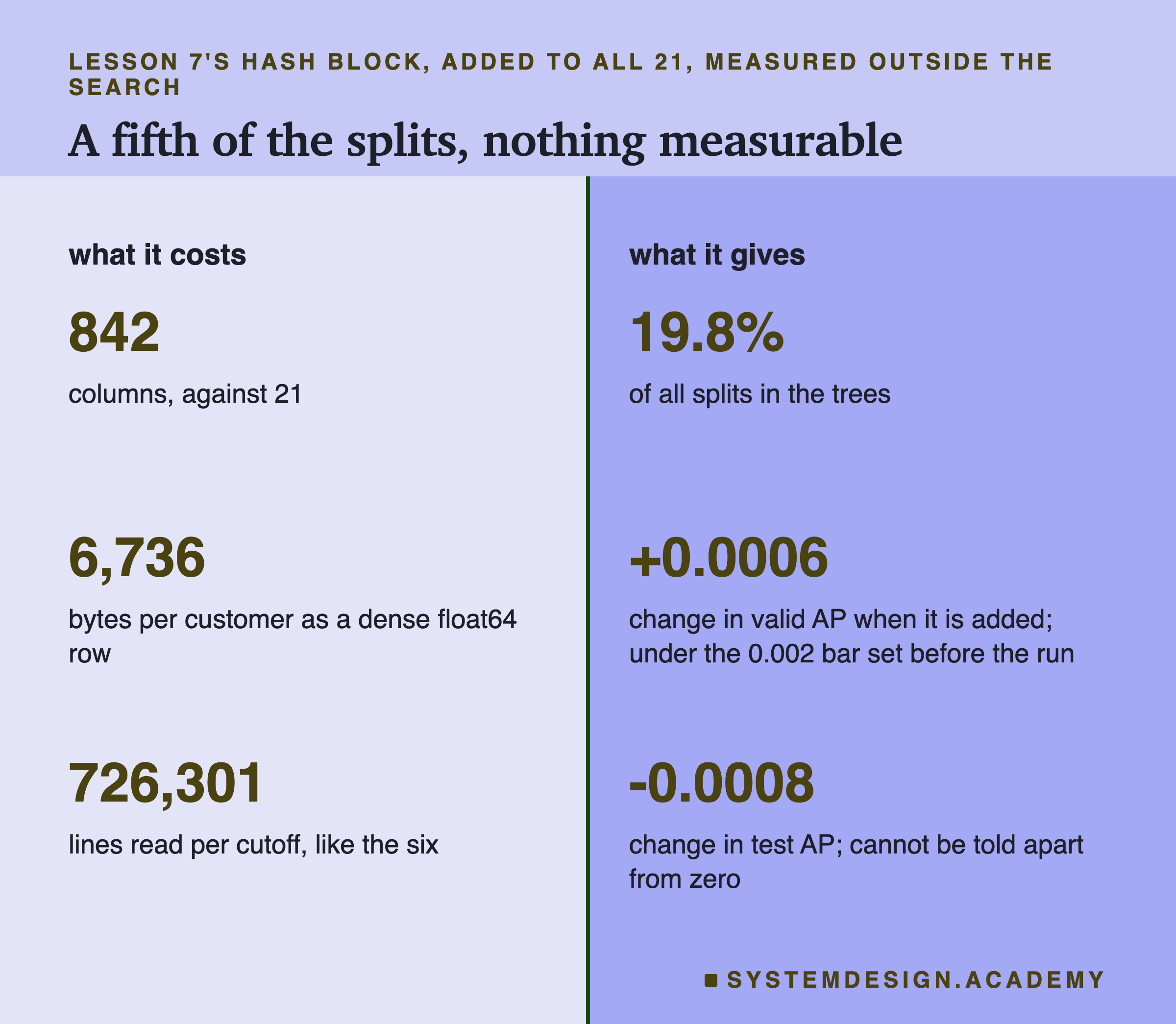
Added to all 21 columns, the hash block took 19.8 percent of all splits in the trees, nearly one in five. By split count, it looks busy. By split gain, it took 4.3 percent. Shuffling the whole block at once cost 0.0028 of valid AP.

But training with and without it, the change in valid AP was +0.0006. That is under the 0.002 bar I set before the run, and I did not bootstrap it. On the test months it was -0.0008, interval -0.0023 to +0.0007, which cannot be told apart from zero.

Lesson 7 measured a small gain for this same block when it was added to the six, with an interval from +0.0008 to +0.0039. Here, added to 21 columns that already include the window counts, that gain is gone. One possible reason, not tested: what a customer's favourite product says about their habits is mostly already in their recent order counts.

So the block costs 40 times the columns of all 21 together, reads all history, and gives nothing measurable once the windows are present. In this shop, for this model, it does not earn its compute.

Here is what backward elimination looked like on the valid months.

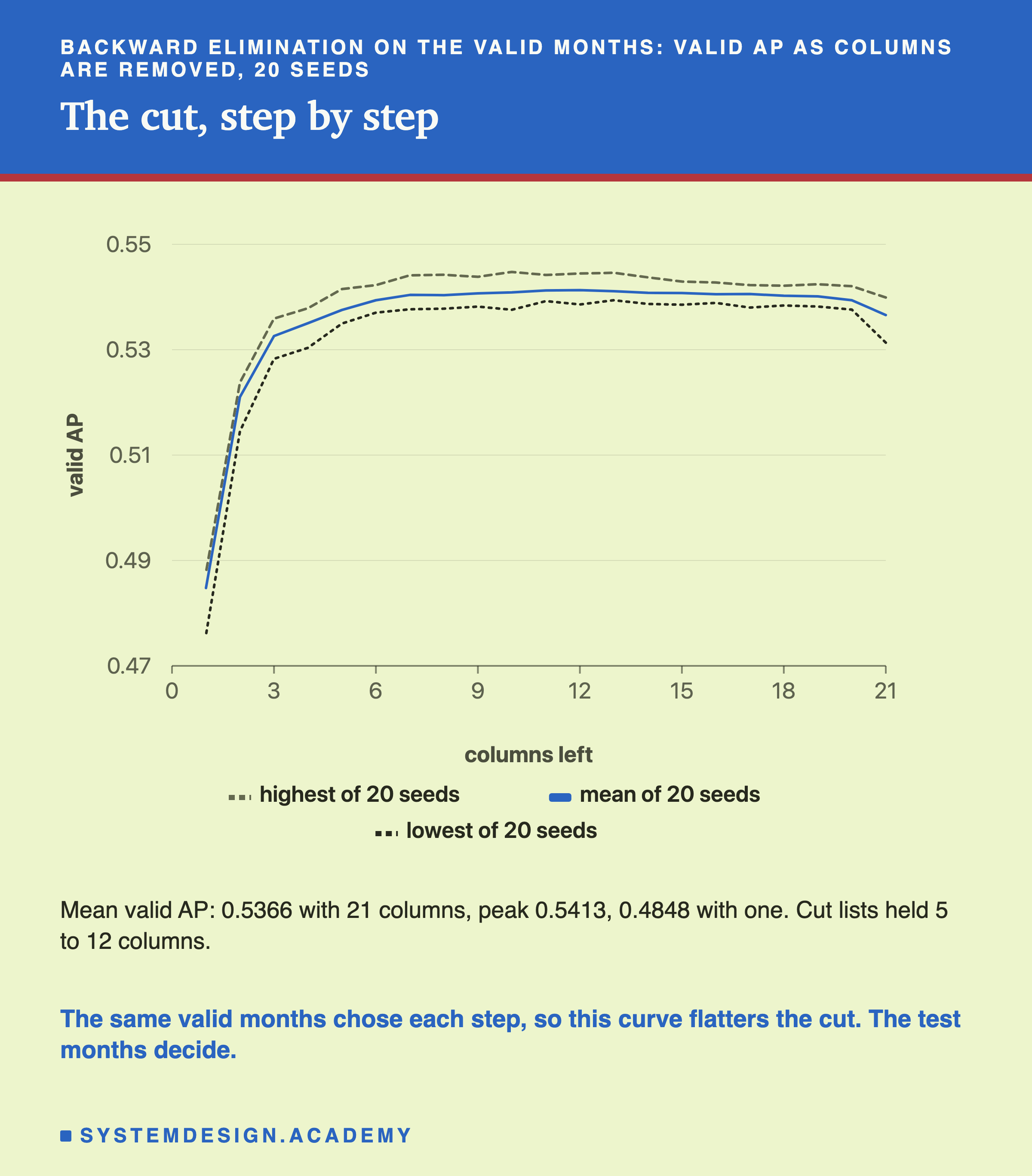
As columns go, valid AP first rises a little, from 0.5366 to a peak of 0.5413 in the mean, and stays flat for a long stretch. It only falls off sharply below three columns.

Please do not read the rise as a gain. Every step was chosen because it gave the highest valid score among its options. So the valid curve is a best case, chosen on the very rows that score it. That is called selection bias. The test months are the honest judge, and there the cut lists' gain was +0.0018, which cannot be told apart from zero.

One more detail. The last column standing was inv_365 in 18 of the 20 seeds and inv_180 in the other 2. In seed 0, recency_days was removed at the step from three columns to two, even though the drop test ranked it first. Greedy steps look only one move ahead.

The task asked me to report how stable the selection was. It was not stable.

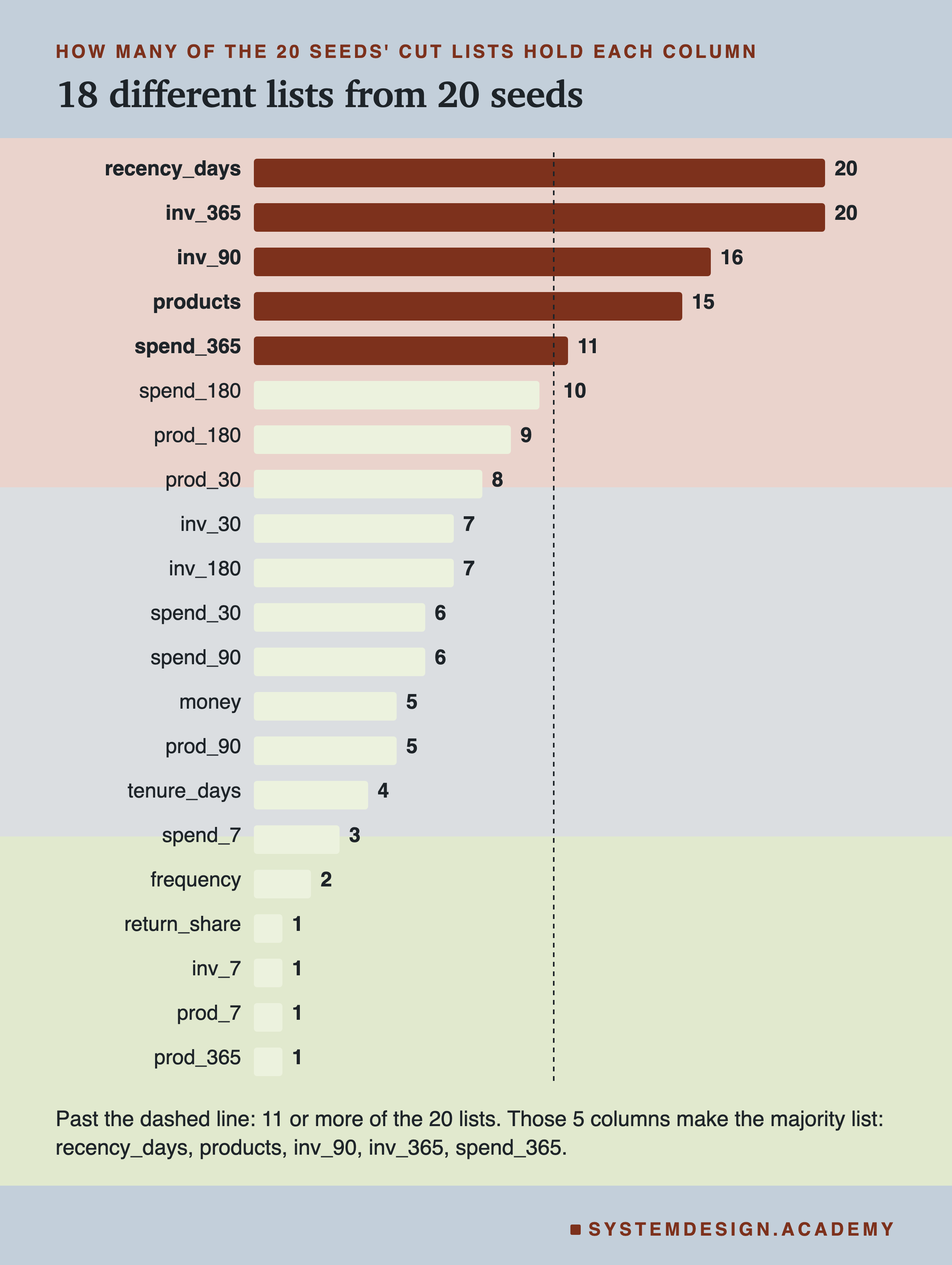
Each seed changes only one thing: which 10 percent of training rows the model holds aside for early stopping. That small change led to 18 different cut lists from 20 seeds. Only one list came up more than once: seeds 9, 18 and 19 all chose the same six columns. Their sizes ran from 5 to 12 columns, and 8 of the 20 had 7. The best-on-valid lists were all 20 different.

Two columns were in every list: recency_days and inv_365. Then inv_90 in 16 and products in 15. frequency, the lifetime order count from lesson 1, made only 2 of the 20 lists, because its twins could always cover for it.

So if you run feature selection once, with one seed, you get one of many possible lists, and the next run may give a different one. What is stable here is not a list. It is a shape: one recency column, one longer order window, and a few more that hardly matter.

That is why I built the majority list, and why I tested it on the test months instead of trusting any one seed.

I wrote six guesses into the lab before it ran. Here they are, against the results.

1. "Permutation importance of frequency alone and of money alone are each under 0.002, and permuting each family as one group costs more than the sum of its parts." Half wrong. Frequency alone was 0.0039 and money alone 0.0053, both above 0.002. The second half held: the frequency family shuffled together cost 0.2660, against 0.2507 for its parts added up, and money's 0.0534 against 0.0474.

2. "Dropping A alone and dropping B alone each cannot be told apart from zero for frequency and money; dropping both is measurably below all 21 for at least one of them." Right for frequency. Wrong for money, where each part alone was measurable and the pair was not.

3. "recency_days has the largest importance by all three measures." Wrong. It was largest only by the drop test. By shuffle and by split gain, inv_180 was far ahead.

4. "The chosen subsets hold 4 to 10 columns, and differ between seeds (more than 5 distinct subsets)." Partly wrong. They held 5 to 12, and 4 of them held 11 or 12. They did differ: 18 distinct lists.

5. "Selected cannot be told apart from all21 on test; all21 is measurably above six; selected is measurably above six." Right on all three.

6. "The hash block's drop-column importance is under 0.002." Right: +0.0006.

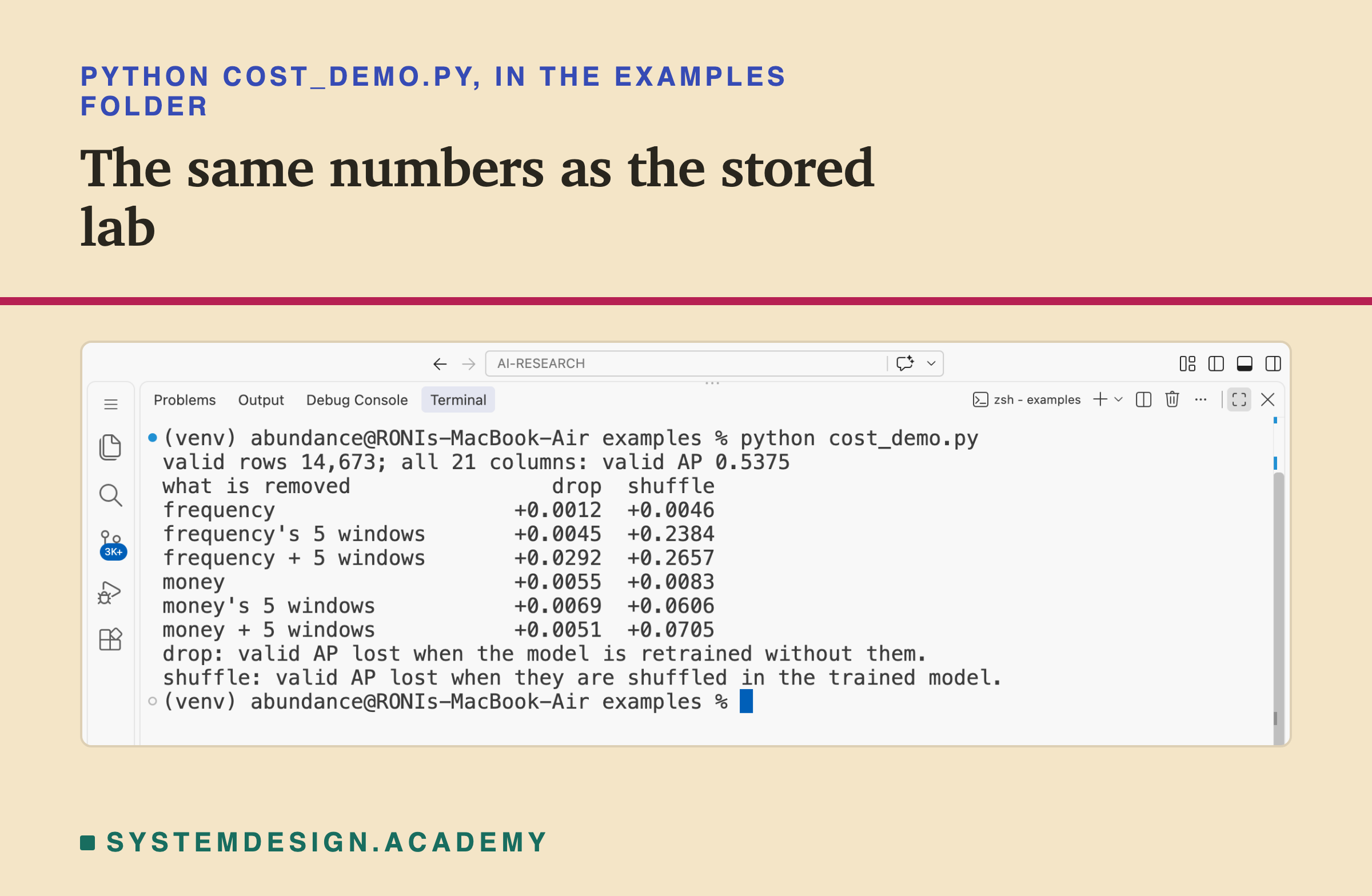
The full lab trains 230 models for each of 20 seeds. I wrote a small demo that shows the twins effect in one go, at seed 0.

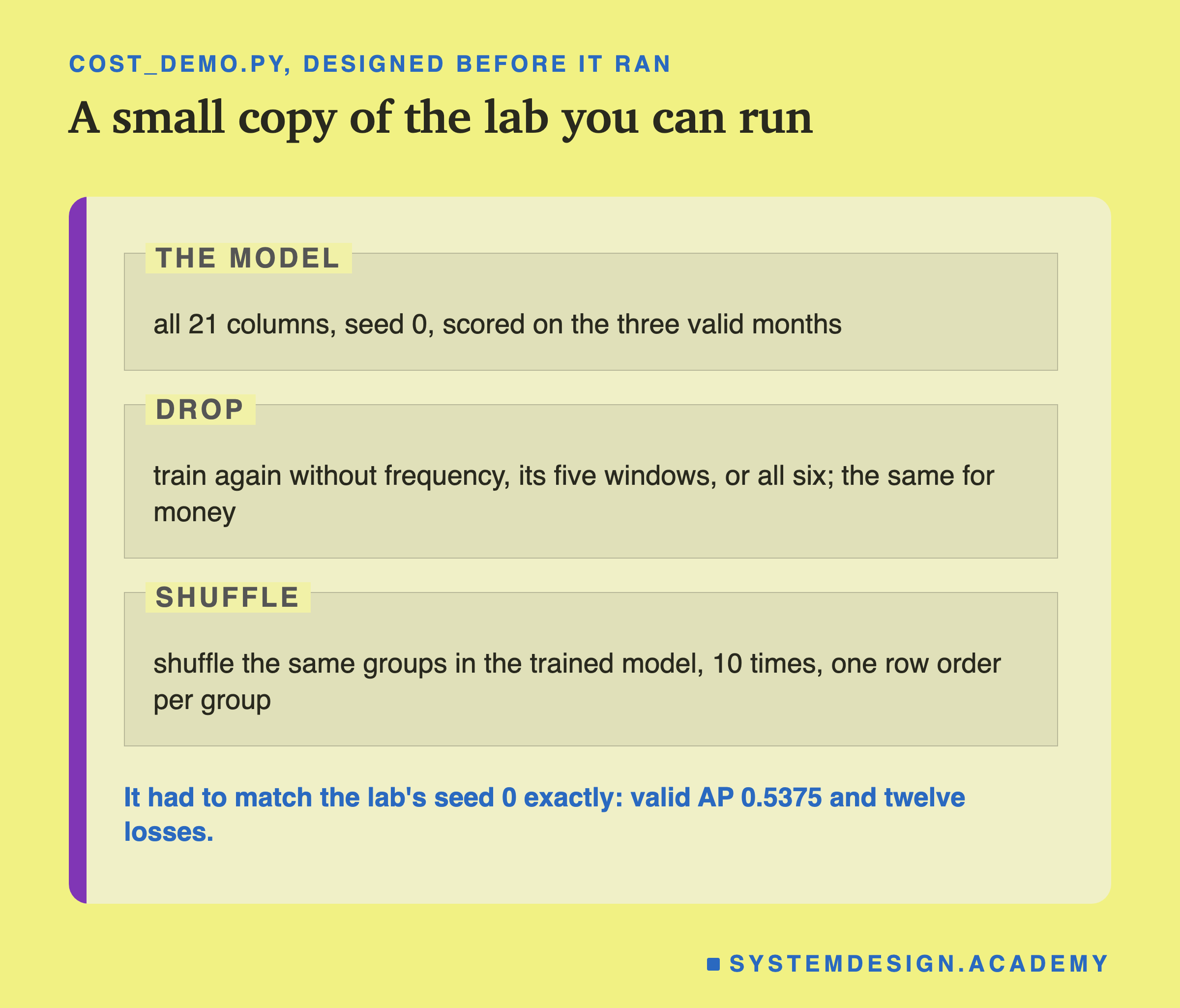
I wrote the demo's design into its docstring after the lab had started and before the demo first ran. Its code is shorter than the lab's and written separately, so it is also a second check of the lab's seed 0.

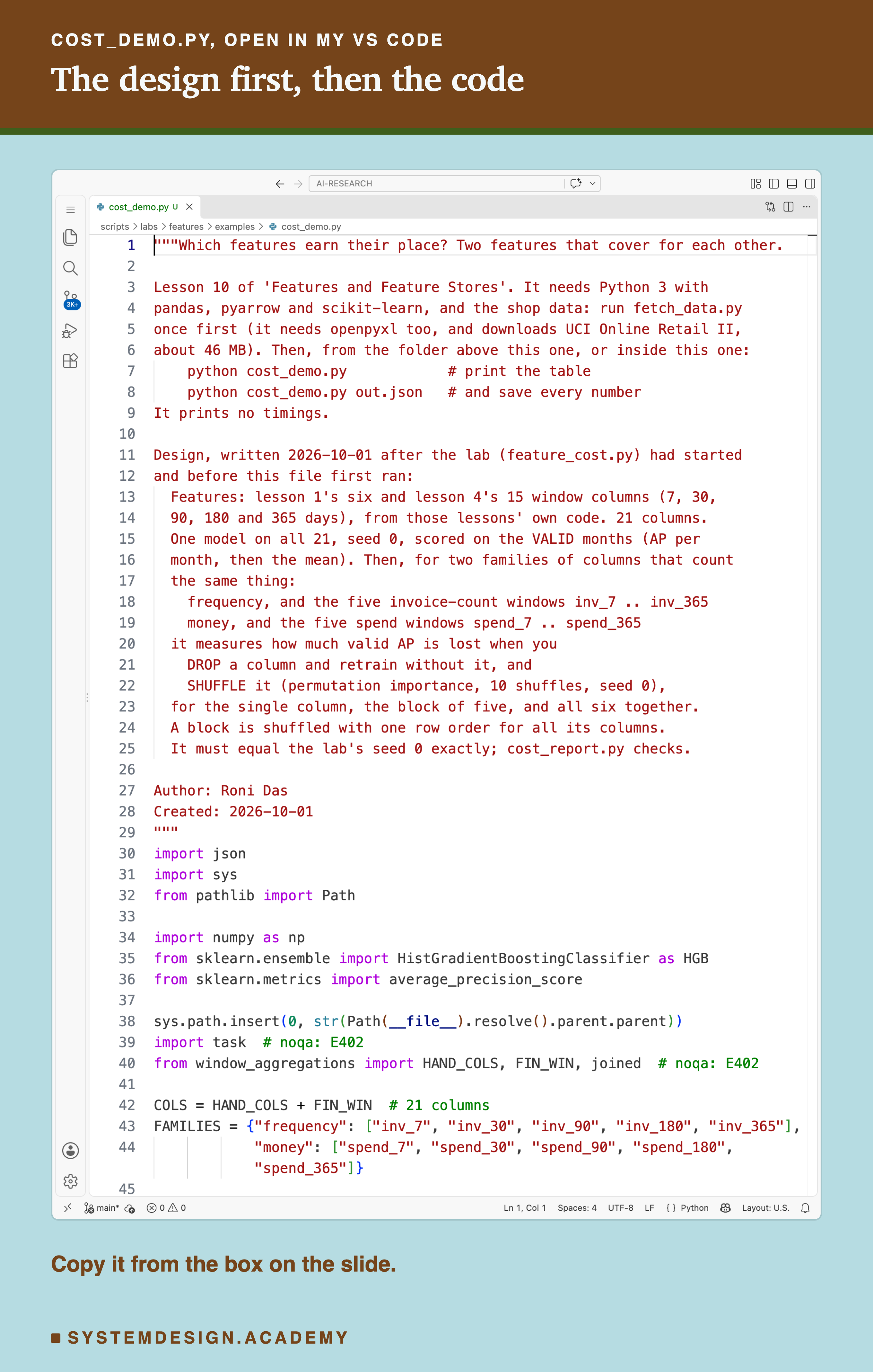
Before you run this lab. You need Python 3 with pandas, pyarrow and scikit-learn: pip install pandas pyarrow scikit-learn openpyxl. First run python fetch_data.py from the scripts/labs/features folder. It downloads the shop data once, about 46 MB, and writes one cleaned file.

The demo imports lesson 4's lab file, window_aggregations.py, which itself imports lesson 1's, from that same folder. It needs no GPU. I ran it with scikit-learn 1.9.1 and pandas 3.0.6 on a Mac, while other programs were using the machine, so I give no time for it. These libraries run on Windows and Linux too, but I have not checked the numbers there. Give it a file name, python cost_demo.py out.json, and it also saves every number. That is how results/cost-demo.json was made.

"""Which features earn their place? Two features that cover for each other.

Lesson 10 of 'Features and Feature Stores'. It needs Python 3 with
pandas, pyarrow and scikit-learn, and the shop data: run fetch_data.py
once first (it needs openpyxl too, and downloads UCI Online Retail II,
about 46 MB). Then, from the folder above this one, or inside this one:
    python cost_demo.py            # print the table
    python cost_demo.py out.json   # and save every number
It prints no timings.

Design, written 2026-10-01 after the lab (feature_cost.py) had started
and before this file first ran:
  Features: lesson 1's six and lesson 4's 15 window columns (7, 30,
  90, 180 and 365 days), from those lessons' own code. 21 columns.
  One model on all 21, seed 0, scored on the VALID months (AP per
  month, then the mean). Then, for two families of columns that count
  the same thing:
    frequency, and the five invoice-count windows inv_7 .. inv_365
    money, and the five spend windows spend_7 .. spend_365
  it measures how much valid AP is lost when you
    DROP a column and retrain without it, and
    SHUFFLE it (permutation importance, 10 shuffles, seed 0),
  for the single column, the block of five, and all six together.
  A block is shuffled with one row order for all its columns.
  It must equal the lab's seed 0 exactly; cost_report.py checks.

Author: Roni Das
Created: 2026-10-01
"""
import json
import sys
from pathlib import Path

import numpy as np
from sklearn.ensemble import HistGradientBoostingClassifier as HGB
from sklearn.metrics import average_precision_score

sys.path.insert(0, str(Path(__file__).resolve().parent.parent))
import task  # noqa: E402
from window_aggregations import HAND_COLS, FIN_WIN, joined  # noqa: E402

COLS = HAND_COLS + FIN_WIN  # 21 columns
FAMILIES = {"frequency": ["inv_7", "inv_30", "inv_90", "inv_180", "inv_365"],
            "money": ["spend_7", "spend_30", "spend_90", "spend_180", "spend_365"]}

ev = task.load_events()
lab_tr, lab_va, _ = task.splits(ev)
tr = joined(ev, lab_tr, task.TRAIN_CUTOFFS)
va = joined(ev, lab_va, task.VALID_CUTOFFS)
months = [np.flatnonzero(va["cutoff"].to_numpy() == t) for t in sorted(va["cutoff"].unique())]
y_va = va["label"].to_numpy()


def score(model, x, y):
    """Valid AP: per month, then the mean of the three months."""
    p = model.predict_proba(x)[:, 1]
    return float(np.mean([average_precision_score(y[m], p[m]) for m in months]))


def valid_ap(cols):
    """Retrain on these columns only (seed 0), score on the valid months."""
    m = HGB(random_state=0).fit(tr[cols].to_numpy(float), tr["label"])
    return score(m, va[cols].to_numpy(float), y_va)


def shuffle_loss(model, cols):
    """Permutation importance of a group: scikit-learn's loop, one row order."""
    x = va[COLS].to_numpy(float)
    j = [COLS.index(c) for c in cols]
    rs = np.random.RandomState(np.random.RandomState(0).randint(2**31))
    base, xp, order, losses = score(model, x, y_va), x.copy(), np.arange(len(x)), []
    for _ in range(10):
        rs.shuffle(order)
        xp[:, j] = xp[np.ix_(order, j)]
        losses.append(base - score(model, xp, y_va))
    return float(np.mean(losses))


full = HGB(random_state=0).fit(tr[COLS].to_numpy(float), tr["label"])
base = score(full, va[COLS].to_numpy(float), y_va)
print(f"valid rows {len(va):,}; all 21 columns: valid AP {base:.4f}")
print(f"{'what is removed':26s} {'drop':>8s} {'shuffle':>8s}")
out = {"valid_ap_all21": base}
for a, block in FAMILIES.items():
    for name, cols in ((a, [a]), (f"{a}'s 5 windows", block), (f"{a} + 5 windows", [a] + block)):
        drop = base - valid_ap([c for c in COLS if c not in cols])
        shuf = shuffle_loss(full, cols)
        out[name] = {"drop": drop, "shuffle": shuf}
        print(f"{name:26s} {drop:+8.4f} {shuf:+8.4f}")
print("drop: valid AP lost when the model is retrained without them.")
print("shuffle: valid AP lost when they are shuffled in the trained model.")
if len(sys.argv) > 1:
    json.dump(out, open(sys.argv[1], "w"), indent=1)

This box holds the lab's real backward elimination paths. For each of the 20 seeds, it has every step from 21 columns down to 1, with its valid AP and the column removed. It also holds how many lines each column reads. It needs nothing but Python, so it runs in your browser.

Press Run. With TOL = 0.002, the box picks the same list at every seed that the lab picked, and counts how often each column is kept. Then try TOL = 0.0, which picks the list with the very best valid score, and watch the lists grow. Try TOL = 0.005, and watch them shrink. Set BUDGET = 1_000_000 to allow at most one million lines per cutoff, and see which columns survive when every all-history column is too expensive. Set SEED = 0 to print one seed's whole path.

The report script writes this box from the lab's stored results. It checks that, with TOL = 0.002 and no budget, the box picks exactly the lab's cut list at all 20 seeds, and with TOL = 0.0 exactly the best-on-valid list. Remember that every number in the box is a valid-month number, chosen on the same months, so it flatters the cut. Only the lab's test numbers, printed at the end, are honest about it.

The lab is one file, scripts/labs/features/feature_cost.py. It imports lessons 1, 4 and 7's feature code instead of copying it. It then checks that all 21 columns reproduce lesson 4's stored scores at all 20 seeds. It also checks that the six reproduce lesson 1's score, and the six plus the hash block lesson 7's.

build joins the three lessons' tables and checks that their rows line up customer by customer. It saves the matrices once, so the 20 seeds can run in four worker processes.

run_seed does everything for one seed. It trains on all 21 columns, then runs the backward elimination, storing every candidate's valid AP. The first step of that search is exactly the drop-column importance, so it costs nothing extra. Then it drops each family's window block and the whole family, runs scikit-learn's permutation_importance with a scorer that averages AP per month, and reads the split record.

permute_group shuffles a group of columns with one row order. It copies scikit-learn's own shuffling loop, and the lab checks that on a group of one column it gives exactly scikit-learn's numbers.

split_record walks the fitted trees through the private _predictors attribute and adds up splits and gain per column.

cost_counts counts lines read and groups formed for each column at one cutoff. timing is the clock, which records the machine's load. holds the two post-results questions.

Deleting a feature because its shuffle importance is high or low. Here the column with the highest shuffle importance, inv_180, could be deleted for nothing. And frequency, with a small one, was half of a pair that mattered a lot.

Trusting split gain because it is free. The trees gave inv_180 more than half of all gain, and the hash block a fifth of all splits. Neither was needed.

Testing twins one at a time. Frequency alone and its windows alone each looked unneeded. Together they were worth 0.0292 of valid AP.

Running the cut once, with one seed. 20 seeds gave 18 different lists.

Reading the valid curve as the result. Every step was chosen on the valid months, so the valid score of the cut list is a best case.

When to use what, from this lab. Use the drop test, one new model per column, when you plan to stop computing a feature, and drop families together as well as one by one. Use the shuffle as a cheap first look at one model, never as a reason to delete. Use split gain to understand what a trained model did, not what the data needs. Price every feature in work and bytes before you add it, and cut with backward elimination on valid at several seeds, then test once.

These are results for one model on one shop, not laws. A straight-line model could rank these columns quite differently, and I did not test one.

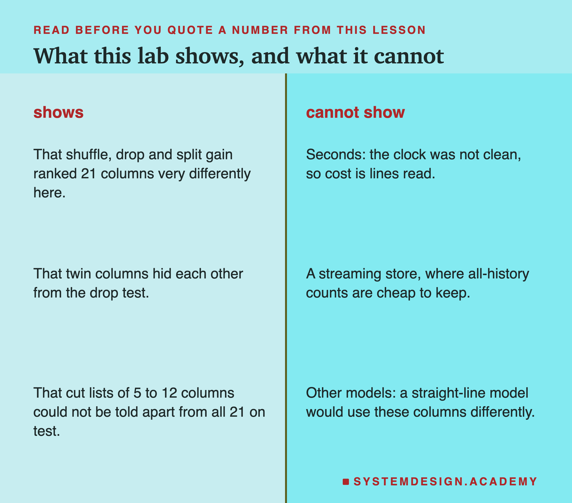
No seconds. The clock was not clean, so cost here is lines read and bytes. Lines read is a fair proxy for a batch job that recomputes each feature from raw events. It is not the same as time.

One cost model. A streaming feature store keeps running counters, so an all-history count costs almost nothing to update, while a 365-day window must also forget old events. Under that model, the six would be cheap and the windows expensive, and the frontier would look different. I named this before the run and did not measure it.

The hash block was outside the search. I measured it separately because of the time it would take inside the search. Inside the search, it might have been cut early, or kept by chance, and I cannot say which.

One model, one shop, a few months. The valid months are three, and the cut was chosen on them. The test months are five. I made two additions after seeing the results: the impossible-row count and the majority-versus-six interval. I made two more after an independent review: the 10-shuffle repeat and the top gain column at every seed. All four are labelled in the lab and on their slides.

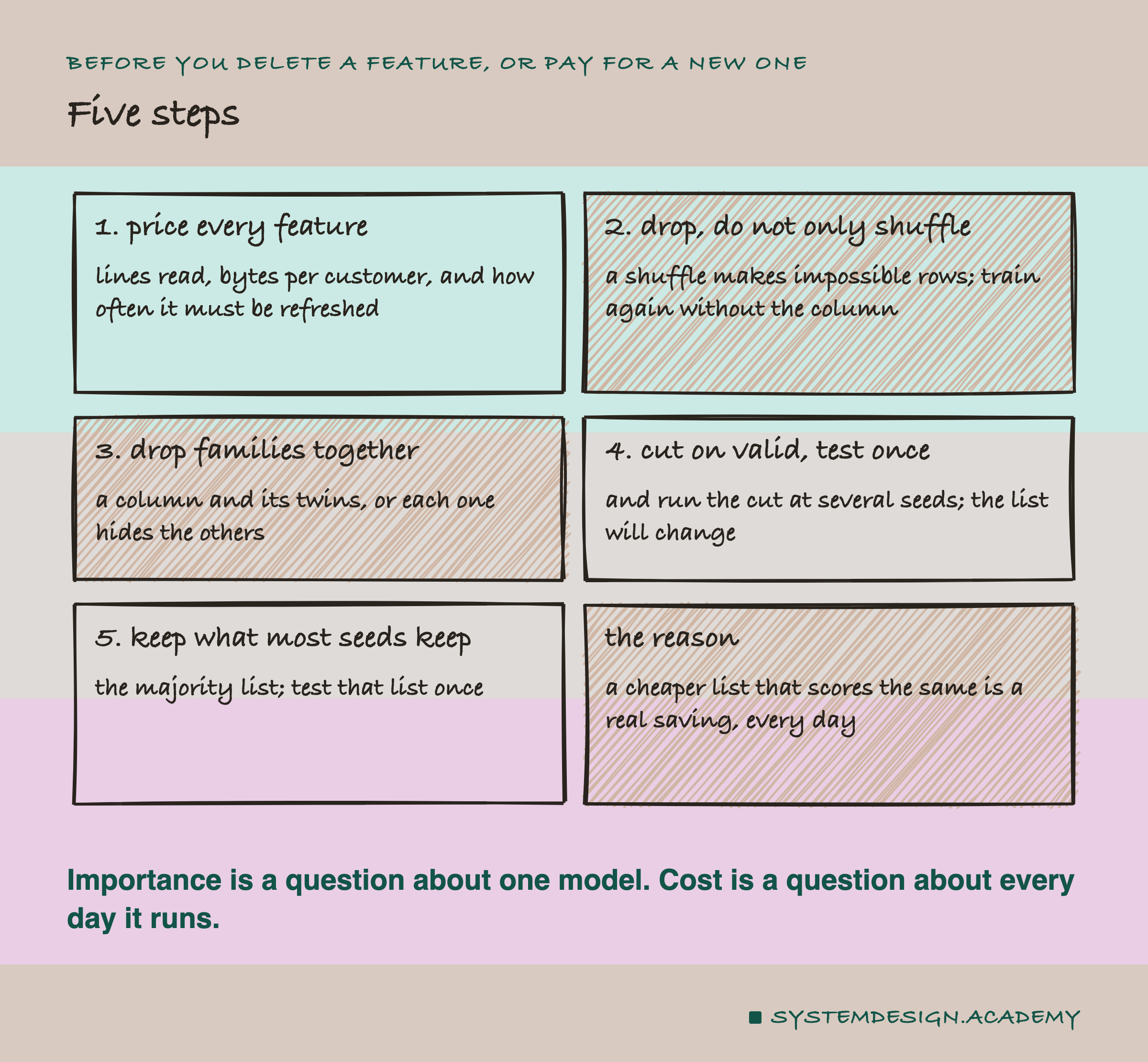
These are the steps I would take the next time a feature list starts to grow, before I add a feature or delete one.

1. Price every feature. Write down what it reads, what it stores, and how often it is refreshed. A feature nobody has priced is a feature nobody can cut.

2. Drop, do not only shuffle. Train a new model without the feature and score it on months the model did not see.

3. Drop families together. Find columns that are twins, by meaning or by correlation, and remove them as a group as well as one by one.

4. Cut on valid, test once, at several seeds. Expect the list to change between seeds, and look at what stays.

5. Keep what most seeds keep (the majority list), and test that list once. Here that list, five columns, scored +0.0001 against all 21, an interval from -0.0039 to +0.0042.