More Cards Than Drawers
Let me start with a small picture.
Imagine a library card cabinet. Every book has a card, and every card must go into a drawer. If the cabinet has one drawer for every book, each card has its own place. But a big library may have thousands of books and only a few dozen drawers.
So the librarian uses a rule. Maybe she files each card by the first letter of the title. Now many cards share a drawer. The rule is quick and the cabinet stays small. But two very different books can end up side by side. A reader who opens the drawer cannot tell them apart without looking closer.

Machine learning has the same problem with columns that hold names instead of amounts. A shop's product code is one. This shop has 4,646 of them. A model needs numbers, so each code must be turned into numbers somehow. You can give every code its own column. You can file codes into a fixed number of drawers. Or you can replace each code with one number learned from the past.
In this lesson I try all three on real data, and two more besides. I count how many codes share a drawer, how much memory each choice needs, and what happens to a code the model has never seen.
Where This Lesson Starts
This lesson uses the same shop, the same customers and the same question as the rest of the chapter. If any of that is new, please read what a feature is first. It sets up the data and the task, and it built six simple features that I reuse here as the starting point.
Those six features were recency, frequency, money, return share, tenure and products. They are all amounts: days, counts and pounds. None of them says WHICH products a customer likes. This lesson asks whether adding that, a column of product names, helps the model, and which way of turning names into numbers works best.
Two earlier lessons matter here. The lesson on point-in-time joins showed what happens when a feature sees past the cutoff. One of the encodings in this lesson did exactly that, by accident, and I only found it after the results came in.
The data engineering lesson on leakage before the split already measured how target encoding leaks when it is done on all the rows at once. I do not repeat that lesson here. This lesson is about scale: thousands of values, names that share a drawer, and names that only appear after training.
The Words You Need First
Please read this slide slowly if any word is new. Every slide after it uses these words.
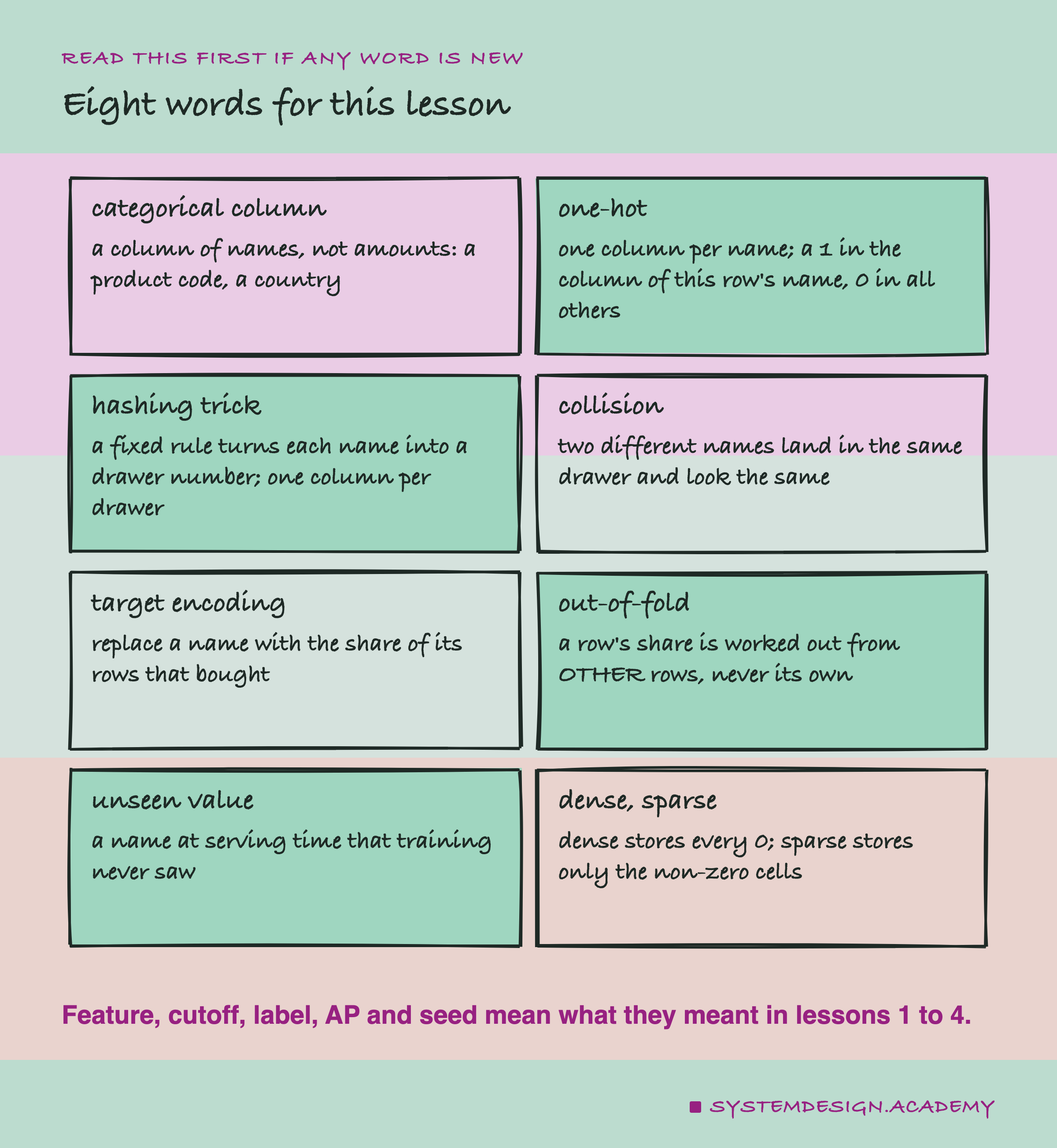
Categorical column. A column that holds names, not amounts. A product code like 85123A is a name. Adding two codes together means nothing, so a model cannot use the code as it is.
One-hot encoding. One new column per name. For each row, the column of that row's name holds a 1 and every other column holds a 0. Like a light switch panel with one switch per name, and only one switch on.
Hashing trick. A fixed rule, called a hash function, turns each name into a number. That number is cut down to a fixed range, so it points at one of a fixed number of buckets, the drawers of the picture. There is one column per bucket.
Collision. Two different names that land in the same bucket. To the model, they then look like the same name.
Target encoding. Replace each name with the share of its rows whose label was 1, here the share of customers with that favourite product who bought again. The word "target" means the label.
Out-of-fold. The rows are split into parts called folds. A row's target encoding is worked out from the other folds only, so its own label is never inside its own number. scikit-learn calls this cross fitting: the encoder is fitted on some folds and used on the fold it did not see.
Unseen value. A name that arrives at serving time but never appeared in training.
Which Categorical Column, and Why
The shop's data has two name columns that could describe a customer: the products they bought, and their country. I had to turn them into one value per row, because a row in this chapter is one customer at one cutoff.
For the product, I chose each customer's favourite code: the stock code on the most purchase lines before the cutoff. Ties go to the code bought most recently, then to the smaller code as text. A customer whose only lines before the cutoff are returns gets the value "none". For the country, I used the country on the customer's last line, exactly as lesson 1 did. So "none" is one of the favourite values too. When I say there are 1,673 favourite codes in the train rows, that count includes "none"; it is the favourite on 311 test rows.
Why one favourite and not every product the customer ever bought? That second choice, which I call the bag, holds more information. But one value per row is the textbook shape of this question: one column with thousands of possible names. With one value per row, all the encodings get exactly the same information, so the race between them is fair. I still measured the bag's size, and I hashed it in two extra contestants, so you can see what the bigger column costs.
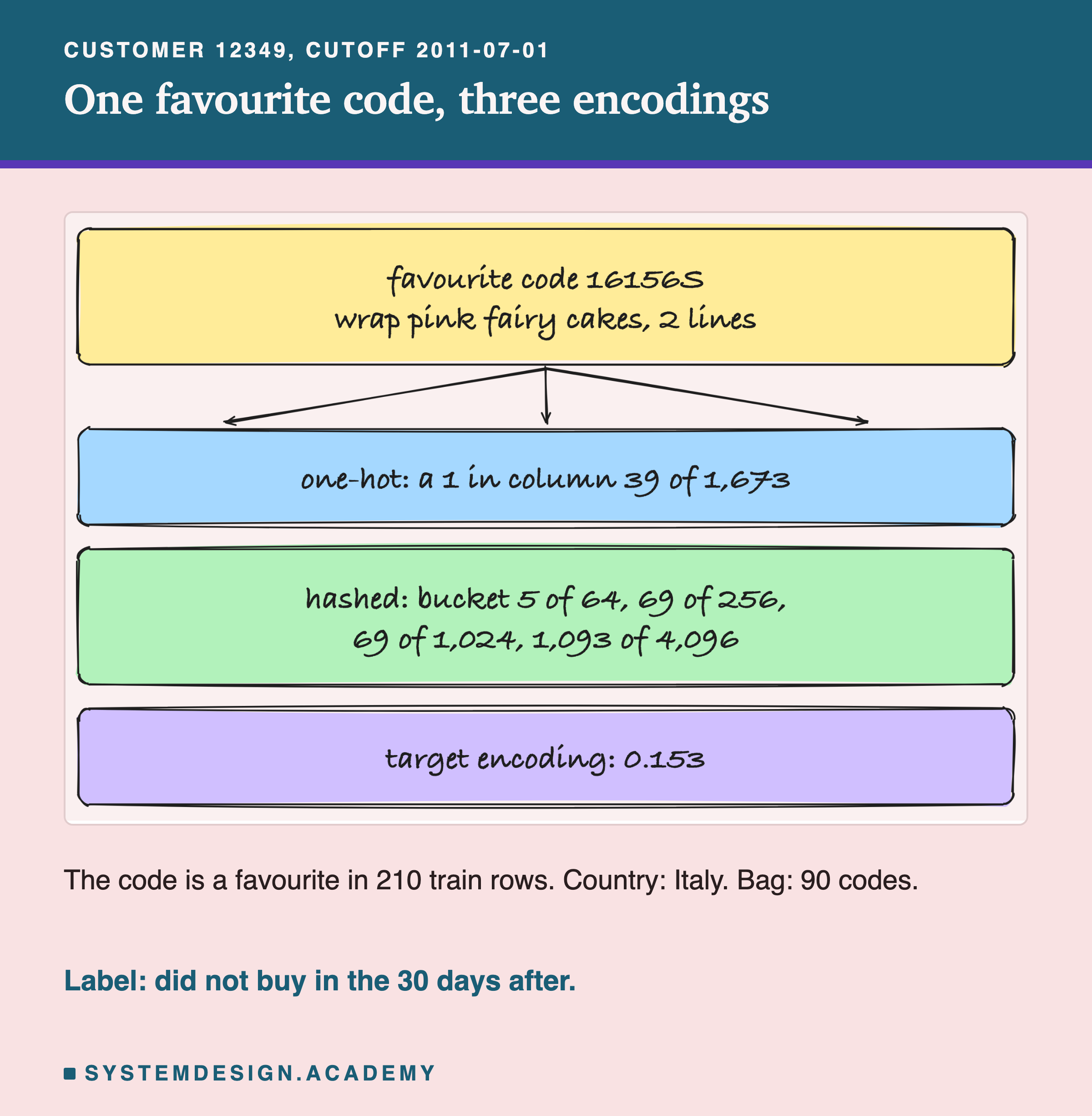
Here is one real customer, number 12349 at the cutoff 1 July 2011, the same customer lessons 1 and 4 used. Their favourite code is 16156S, wrapping paper with pink fairy cakes, on just 2 of their lines. They had bought 90 different codes. The same code is the favourite in 210 train rows, so the model has seen it many times. One-hot puts a 1 in column 39 of 1,673. Hashing puts it in bucket 69 of 1,024. Target encoding, at seed 0, turns it into 0.153.
Three Ways to Turn a Name Into Numbers
The three main encodings give the model very different shapes.
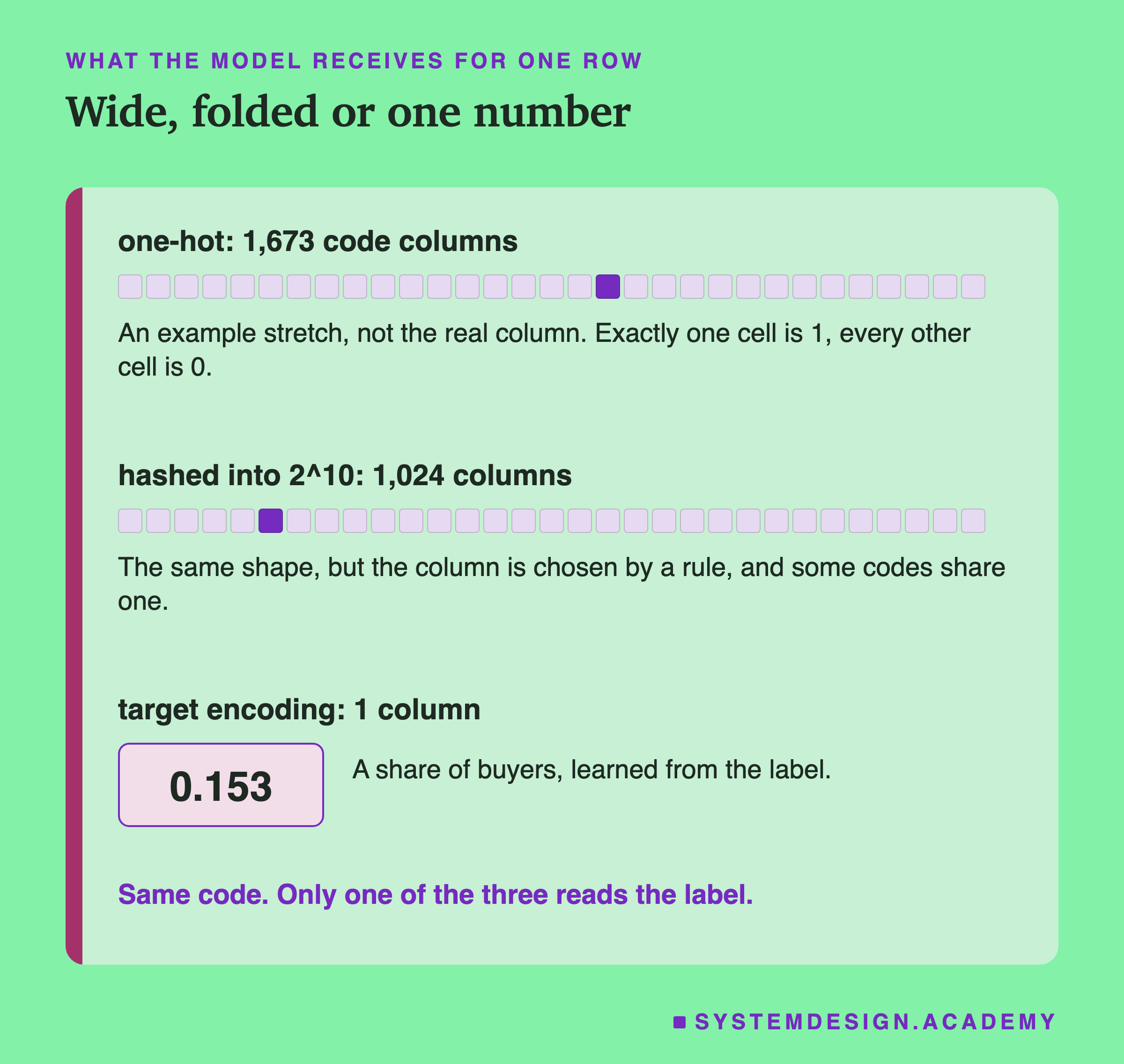
One-hot is wide. Here it made 1,673 code columns, one for every favourite code in the train rows, plus 40 country columns. Every row has a single 1 in the code part. Nothing is lost, but a code that never appeared in training has no column at all.
Hashing is also wide, but you choose the width. scikit-learn's FeatureHasher runs each name through a hash function called MurmurHash3. It turns any text into a big whole number, and the same text always gives the same number. The number is then cut down to the number of buckets with a remainder after division. So "code=16156S" always lands in bucket 69 of 1,024. The hasher never needs to see the training data first. It also has an answer for a code it has never seen: that code lands in some bucket too.
Target encoding is narrow: one column per name column. It is the only one of the three that reads the label. That makes it powerful, because the number already says something about buying. It also makes it dangerous, because a number built from labels can carry a row's own answer into training.
The idea of hashing features is older than any one paper. A well-known paper on it is "Feature Hashing for Large Scale Multitask Learning" by Weinberger, Dasgupta, Langford, Smola and Attenberg, at the ICML conference in 2009. Its new step was a second hash that gives each feature a plus or minus sign, so that collisions tend to cancel out on average. They used it to filter spam for hundreds of thousands of email users at once.
The Shop, the Task and the Split
The data is UCI Online Retail II, a public dataset under a CC BY 4.0 licence. It holds every sale of a UK online shop from 1 December 2009 to 9 December 2011. The shop mainly sells gift items, and many of its customers are wholesalers, people who buy to sell again. The chapter's fixed cleaning drops lines with no customer id and keeps returns as flagged rows.
The task is the chapter's fixed one. On the first of each month, for every customer seen before that day, will they buy in the next 30 days? Each pair of a customer and a cutoff is one row, and the label is 1 if they bought.
The rows are split by time. Train months, March 2010 to March 2011, give 44,521 rows; the models and every encoder learn from these. Valid months, April to June 2011, give 14,673 rows; choices like the smoothing and the number of buckets are made here. Test months, July to November 2011, give 26,851 rows; they only score, and they choose nothing.
Average precision (AP) asks: when the model's list of likely buyers is read from the top, how many of the names near the top really bought? A random list scores about the share of buyers, which averaged 0.196 over the five test months. Every AP in this lesson is worked out per test month and then averaged.
How the Lab Was Built
I wrote the lab's design into the docstring of scripts/labs/features/categorical_scale.py before it first ran. Before that I had looked only at the data's shape and at scikit-learn's own descriptions of the three encoders. I had also timed one model fit on random numbers of the one-hot shape, only to check the run would finish. No model had been trained on this task with any product column.
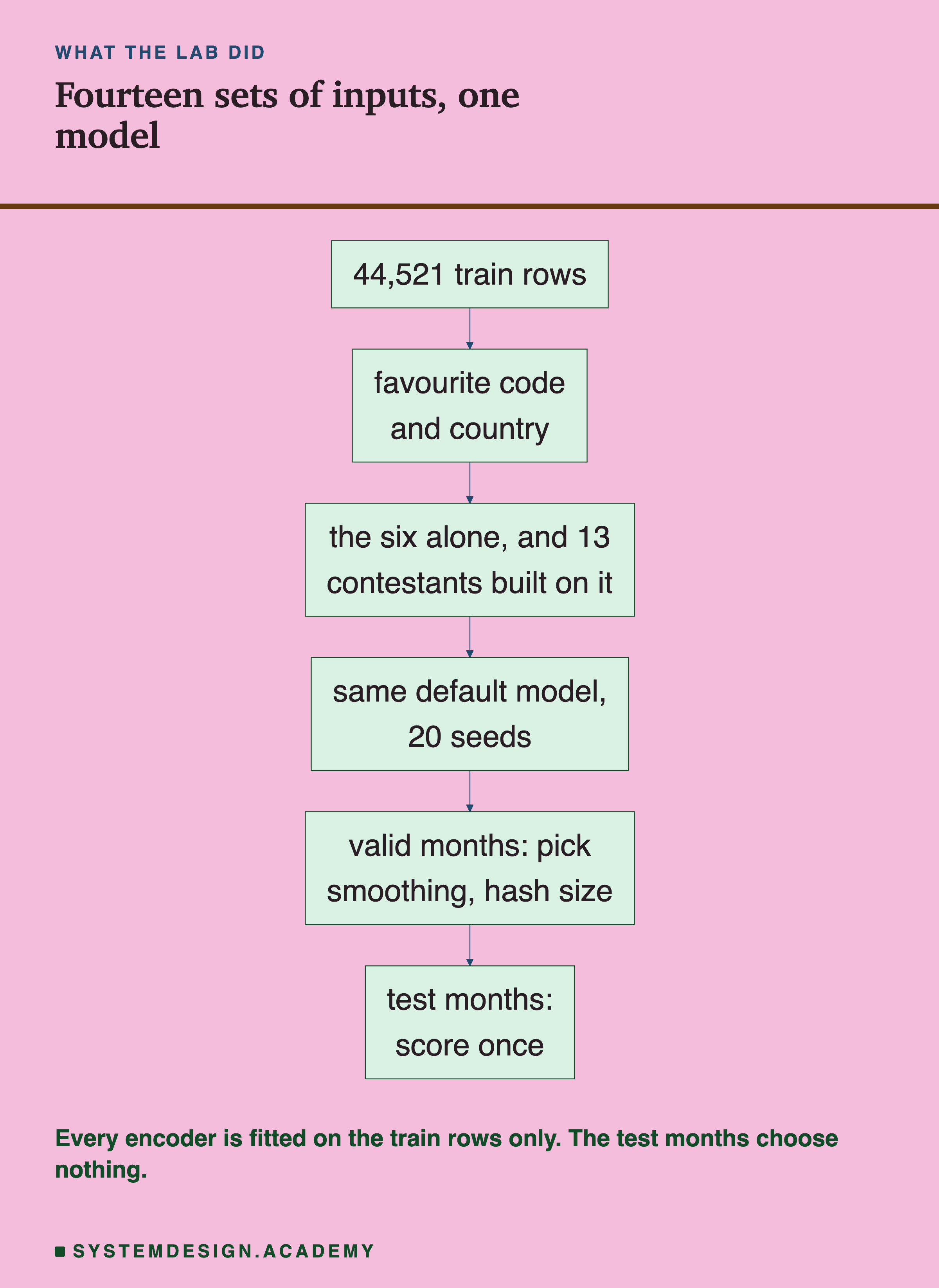
The model is the chapter's usual one: scikit-learn's HistGradientBoostingClassifier with its default settings. It builds many small decision trees, each one fixing the mistakes of the trees before it. Only the inputs change from one contestant to the next.
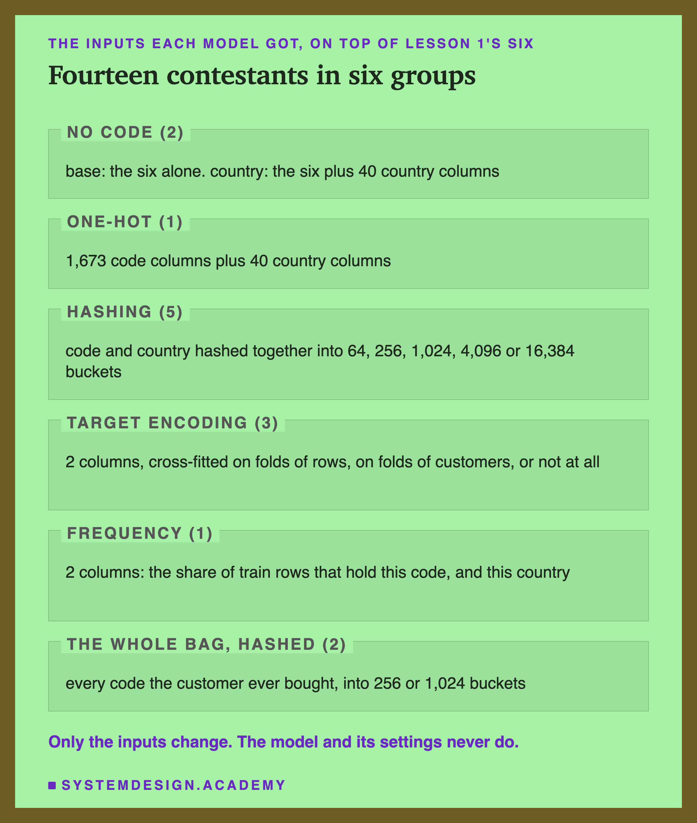
The frequency encoding replaces a name with the share of train rows that hold it. It is cheap and reads no label. I put it in the design as a cheap baseline. Its design had a flaw I only found after the results: it counted over all 13 train months. It turned out to be the biggest story in the lesson.
The design wrote down six guesses so they could be wrong in public. Here they are, scored.
-
Country adds nothing. Right: 0.5452 with country and 0.5452 without.
-
(An interval is a range of likely gaps; the slide How Sure Can I Be explains it.) Wrong twice. One-hot and the three bigger hash sizes did clear zero, just. And target encoding with the usual folds came in below the six.
How Many Codes Share a Bucket
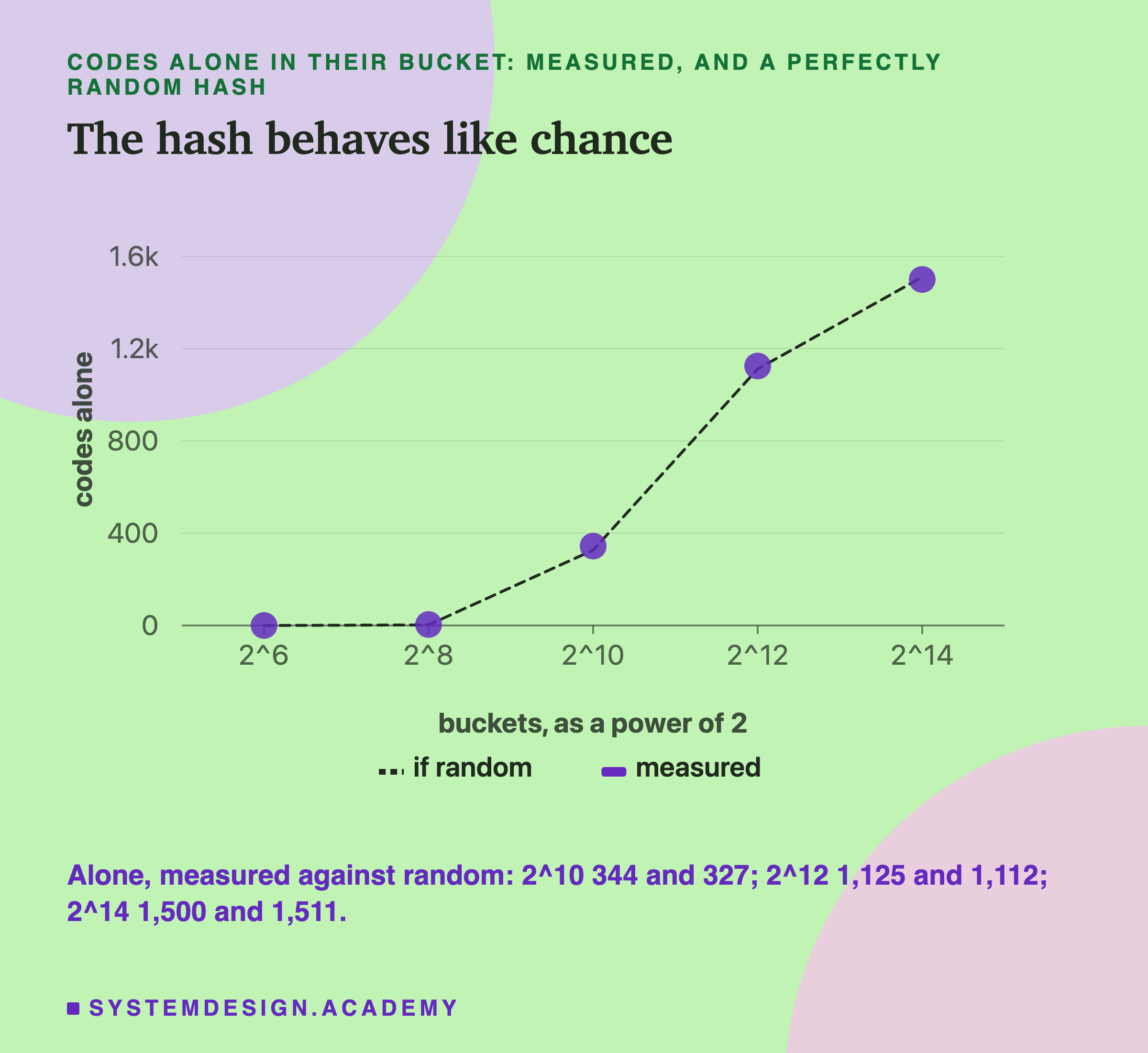
Before any model, the lab counted the collisions. There are 1,673 different favourite codes in the train rows, and I hashed each one at five sizes.
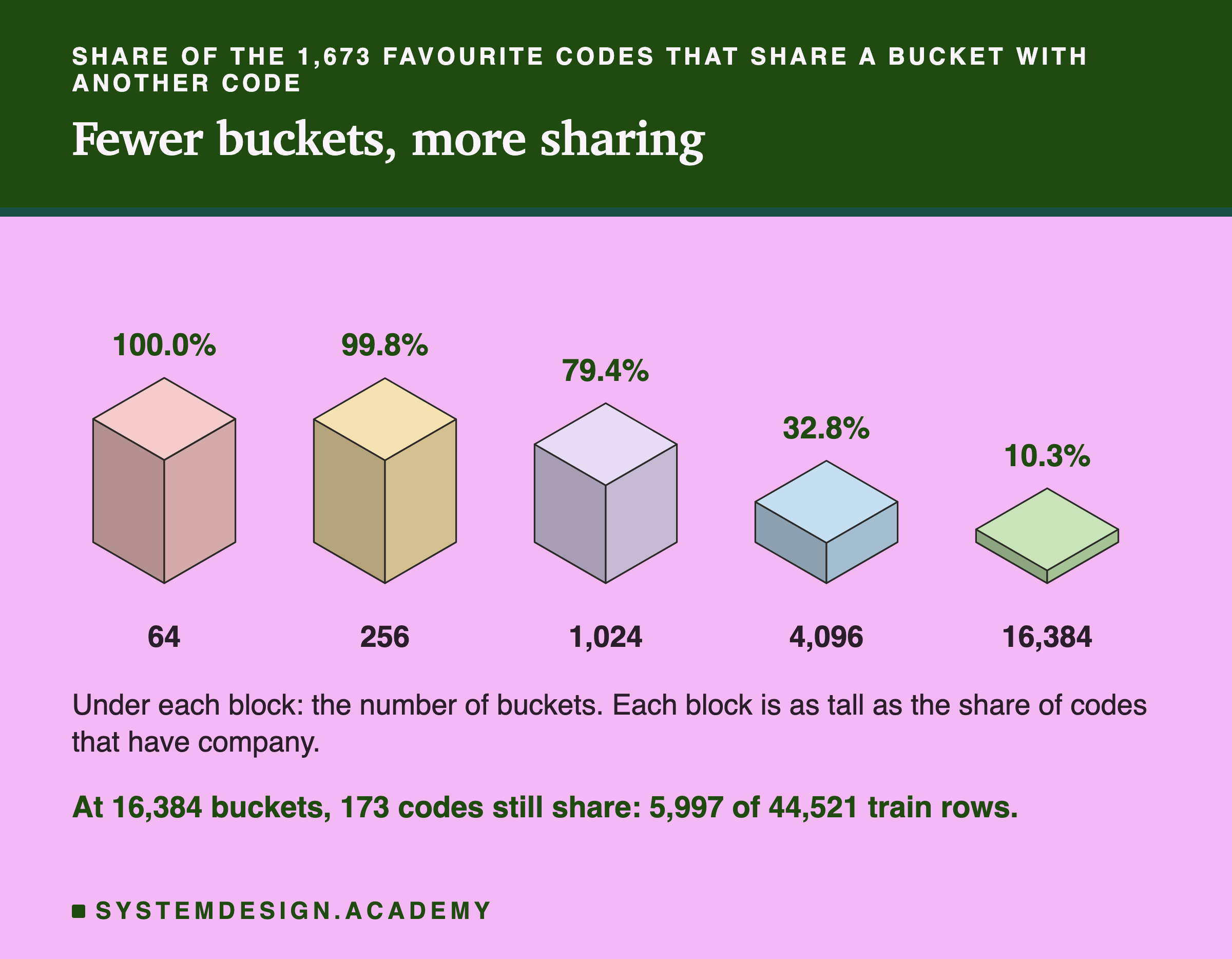
| buckets | codes sharing a bucket | train rows affected | most codes in one bucket |
|---|---|---|---|
| 64 | 1,673 | 44,521 | 37 |
| 256 | 1,669 | 44,485 | 17 |
| 1,024 | 1,329 | 36,539 | 6 |
| 4,096 | 548 | 15,382 | 4 |
| 16,384 | 173 | 5,997 |
The Lab's Report, Running
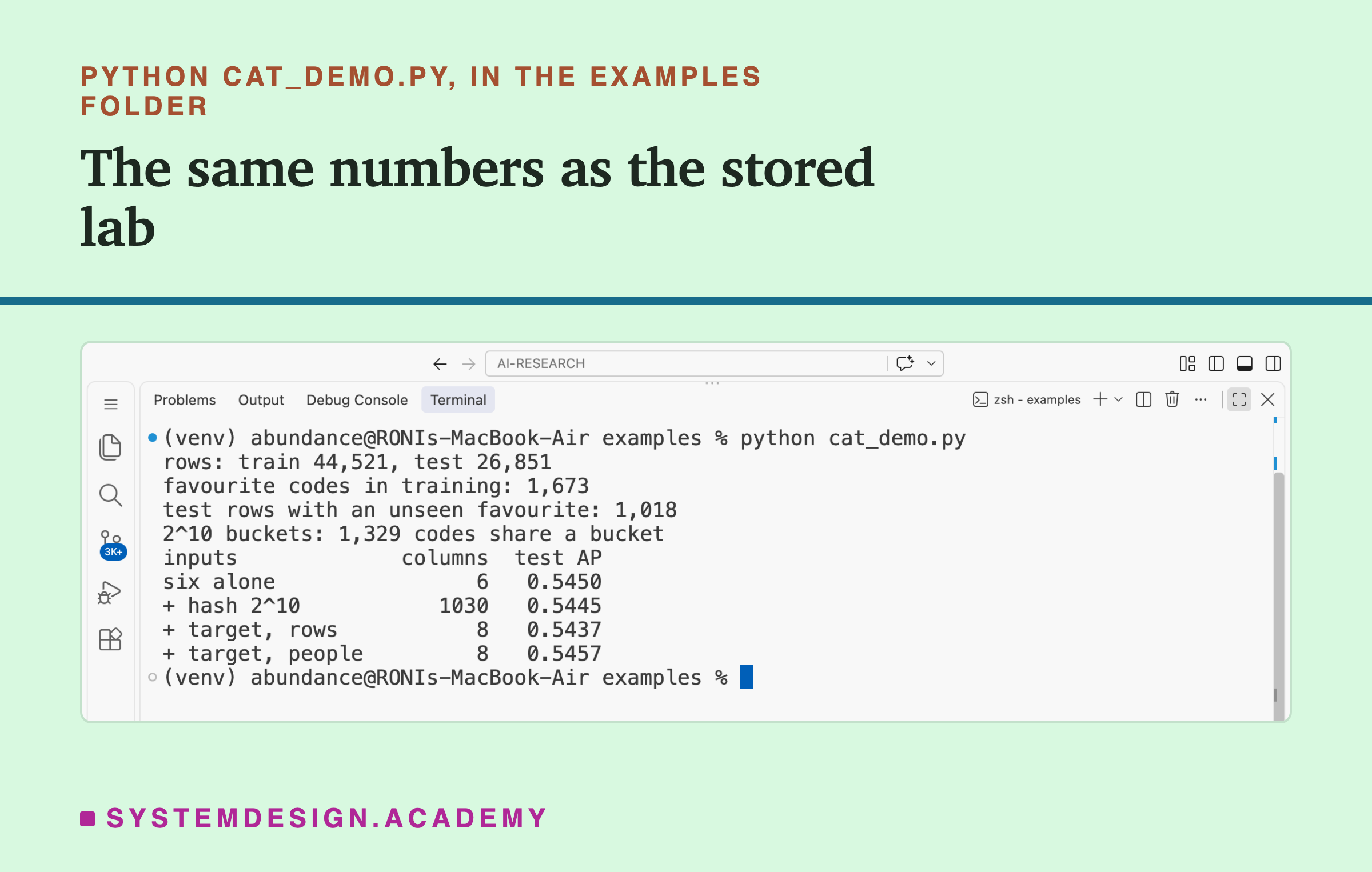
This is a real recording of the report script, cat_report.py, on the laptop where the lab ran. It trains nothing. It reads the stored results and checks every number this lesson uses.
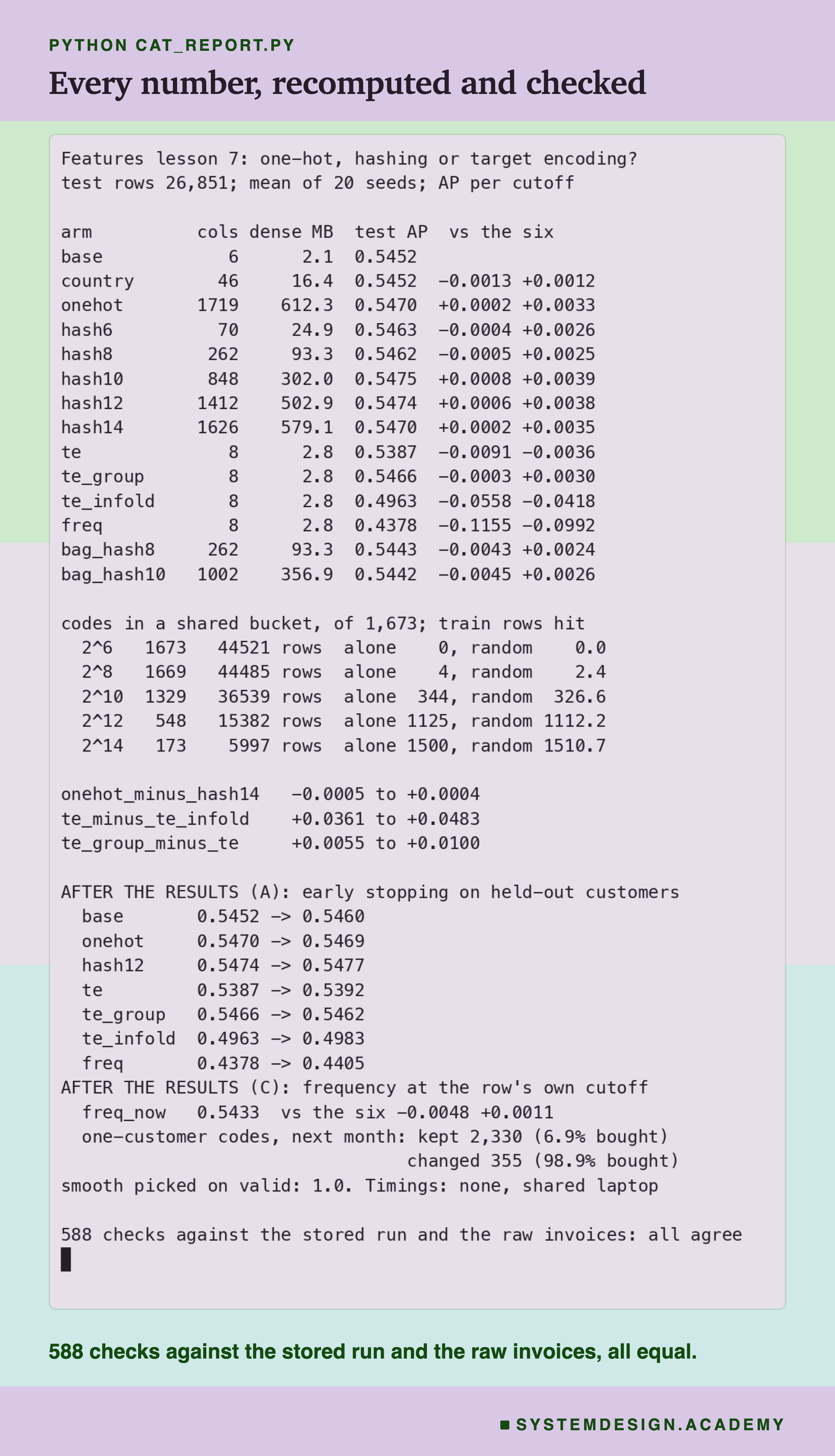
The report rebuilds every row's favourite code from the raw invoices with its own, simpler code. From those it recounts the unseen rows, the bag, and customer 12349's values. It also has its own copy of MurmurHash3, written in plain Python. It checks that this copy puts every code in the same bucket as scikit-learn does, at every size. Then it recounts the collisions with it.
It also checks each mean against the 20 stored seeds, and each interval against its 1,000 stored resamples. It checks the student demo against the lab and the playground box's printout. Last, it checks that every number in this lesson appears in the lesson text. If anything disagrees, it stops with an error.
What Each Encoding Scored
Here is every contestant, scored on the five test months and averaged over 20 training seeds.
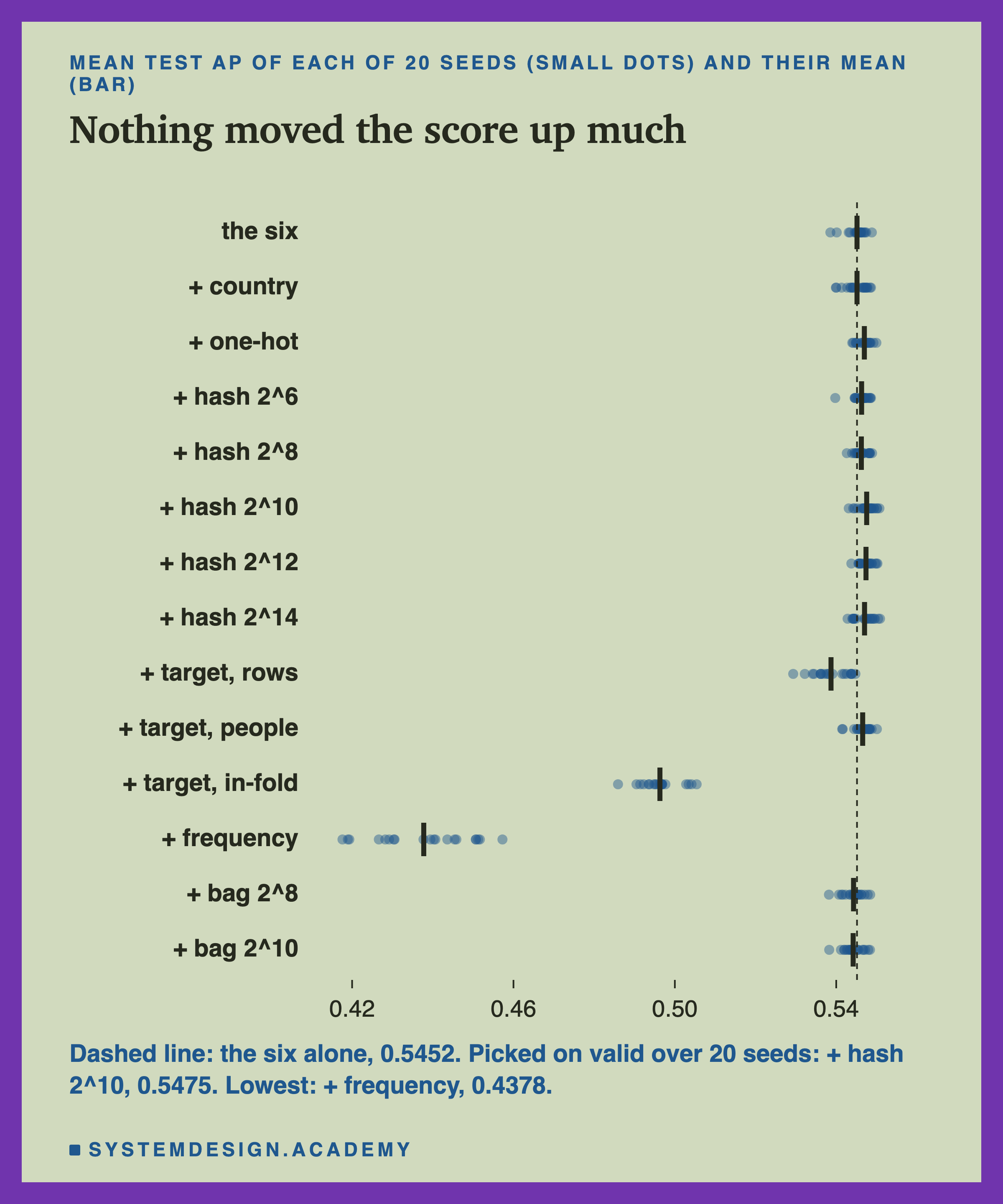
| inputs | columns | test AP | ROC-AUC |
|---|---|---|---|
| the six alone | 6 | 0.5452 | 0.798 |
| + country | 46 | 0.5452 | 0.799 |
| + one-hot | 1,719 | 0.5470 | 0.800 |
| + hash, 64 buckets | 70 | 0.5463 | 0.799 |
| + hash, 256 buckets |
How Sure Can I Be?
Gaps of a few thousandths need care. I checked two kinds of luck.
Luck in training. The model sets aside 10 percent of the train rows at random to decide when to stop adding trees. That is called early stopping, and the seed moves it. So every contestant was trained with 20 seeds, 0 to 19. The six alone ranged from 0.539 to 0.549 over the seeds, a spread several times larger than the best gain. One seed alone would have told almost any story.
Luck in which customers were tested. A bootstrap draws the test customers again at random, with repeats allowed, within each test month. I did that 1,000 times, with the same draws for every contestant, and each time worked out the 20-seed mean AP of each contestant minus the six. The middle 95 percent of those gaps is the 95% interval.
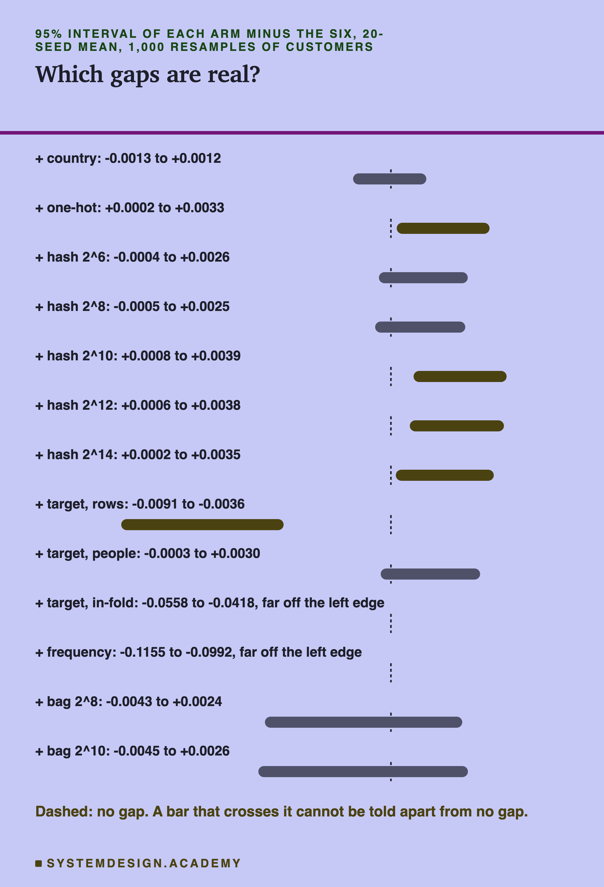
Four gains stayed above zero: one-hot, +0.0002 to +0.0033, and hashing at 1,024, 4,096 and 16,384 buckets. Each is very close to zero at its low end, and one-hot's did not survive a later check. Country, the two small hashes, target encoding on folds of customers and both bag contestants cannot be told apart from the six. Three contestants were clearly worse: target encoding on folds of rows, target encoding with no folds, and frequency.
One-hot against 16,384 buckets: -0.0005 to +0.0004. Those two cannot be told apart. 16,384 buckets against 64: -0.0004 to +0.0020, also not clear.
A confound to keep in mind. The contestants that gained also had far more columns. One-hot had 1,719 against 6. So these numbers cannot say whether the code itself helped, or whether a model with more columns to split on simply found a little more. And a later check, two slides on, found the one-hot gain does not survive a change in how early stopping picks its rows.
What the Width Costs
The scores barely moved. The memory did not.
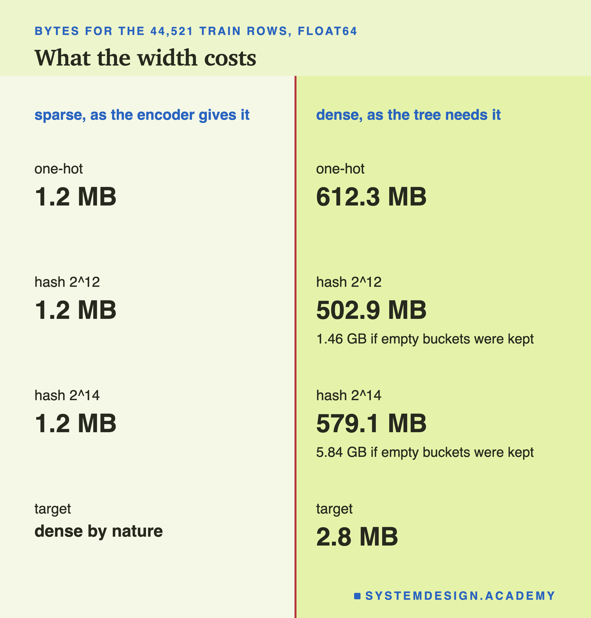
The encoders hand back a sparse table. Each row has only two cells that are not zero, one for the code and one for the country. So the sparse table is about 1.2 MB at every width. Width costs almost nothing when you store only the ones.
The model is a different matter. This kind of tree model in scikit-learn needs a dense table, every cell stored. I checked: given a sparse table, it stops with an error that says dense data is required. One-hot then needs 612.3 MB for the train rows alone. Hashing into 16,384 buckets would need 5.84 GB if the empty buckets were kept; dropping them brought it to 579.1 MB. Target encoding needs 2.8 MB, the same as the six plus two columns. A MB is a million bytes and a GB is a thousand MB.
So the cost of a wide encoding depends on the model. A linear model, which gives each column a weight and adds them up, can read the sparse table as it is. I did not test one. For the tree model here, the width is paid in full.
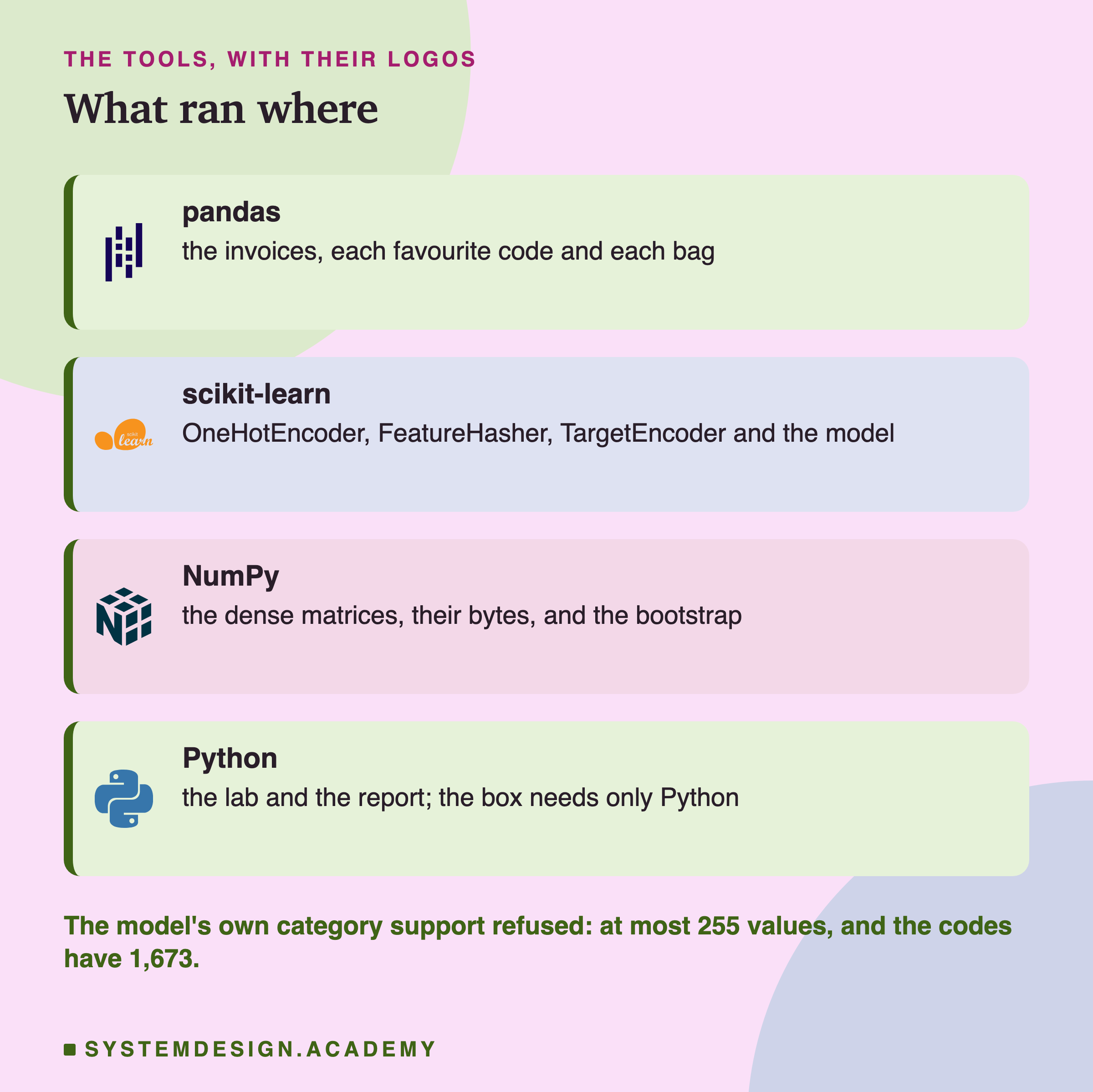
Why not let the tree model handle the codes itself? HistGradientBoostingClassifier has its own support for categorical columns. I tried it on the favourite codes. It stopped with an error: "Categorical feature at index 0 is expected to have a cardinality <= 255 but actually has a cardinality of 1673." Its documentation says each categorical column may have at most max_bins values, and max_bins can be no larger than 255.
The Bag Is the Bigger Column
The favourite is one code per row. The bag, every code the customer ever bought, is much bigger.
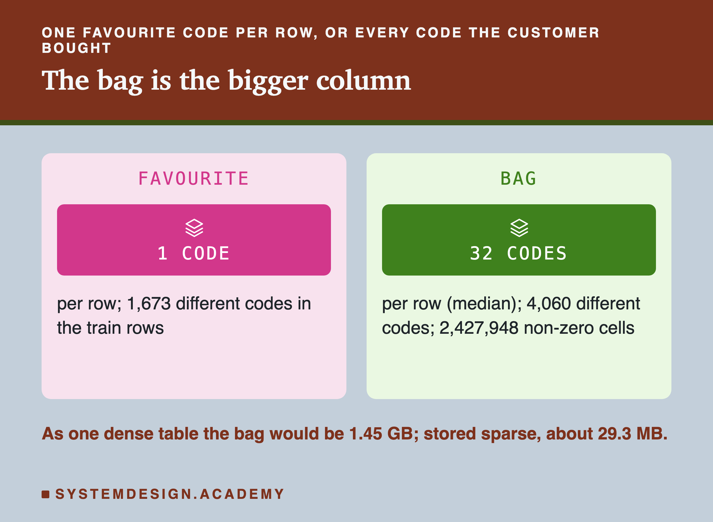
The train rows hold 4,060 different codes in their bags. The middle customer row has 32 codes, and the mean is 54.5, because some wholesalers buy hundreds of products. One-hot over the bag, often called multi-hot because a row can have many ones, would have 2,427,948 non-zero cells in the train rows. Stored dense, it would be 1.45 GB. Stored sparse it would be about 29.3 MB; that figure is worked out from the cell count, not measured from a built table.
I hashed the bag into 256 and 1,024 buckets. At 1,024 buckets, 3,980 of the 4,060 codes share a bucket. Neither bag contestant could be told apart from the six: 0.5443 and 0.5442 against 0.5452.
The bag also has more unseen codes. 10,806 test rows hold at least one code that no train row's bag held. That is 5.7 percent of all the codes in test bags. New products arrive every month, and a customer who buys a lot will buy some of them.
So the bigger column was not the stronger column here. One possible reason, which I did not test: the six already know how much and how often a customer buys, and which products they buy says little extra about whether they come back within a month.
A Code the Model Has Never Seen
At serving time, some customers have a favourite that no train row had. The lab counted them: 1,018 test rows, 3.8 percent. Of those, 289 hold a code the shop had not sold at all before 1 March 2011. The rest are older codes that simply were nobody's favourite in training. Five test rows also had a country that no train row had.
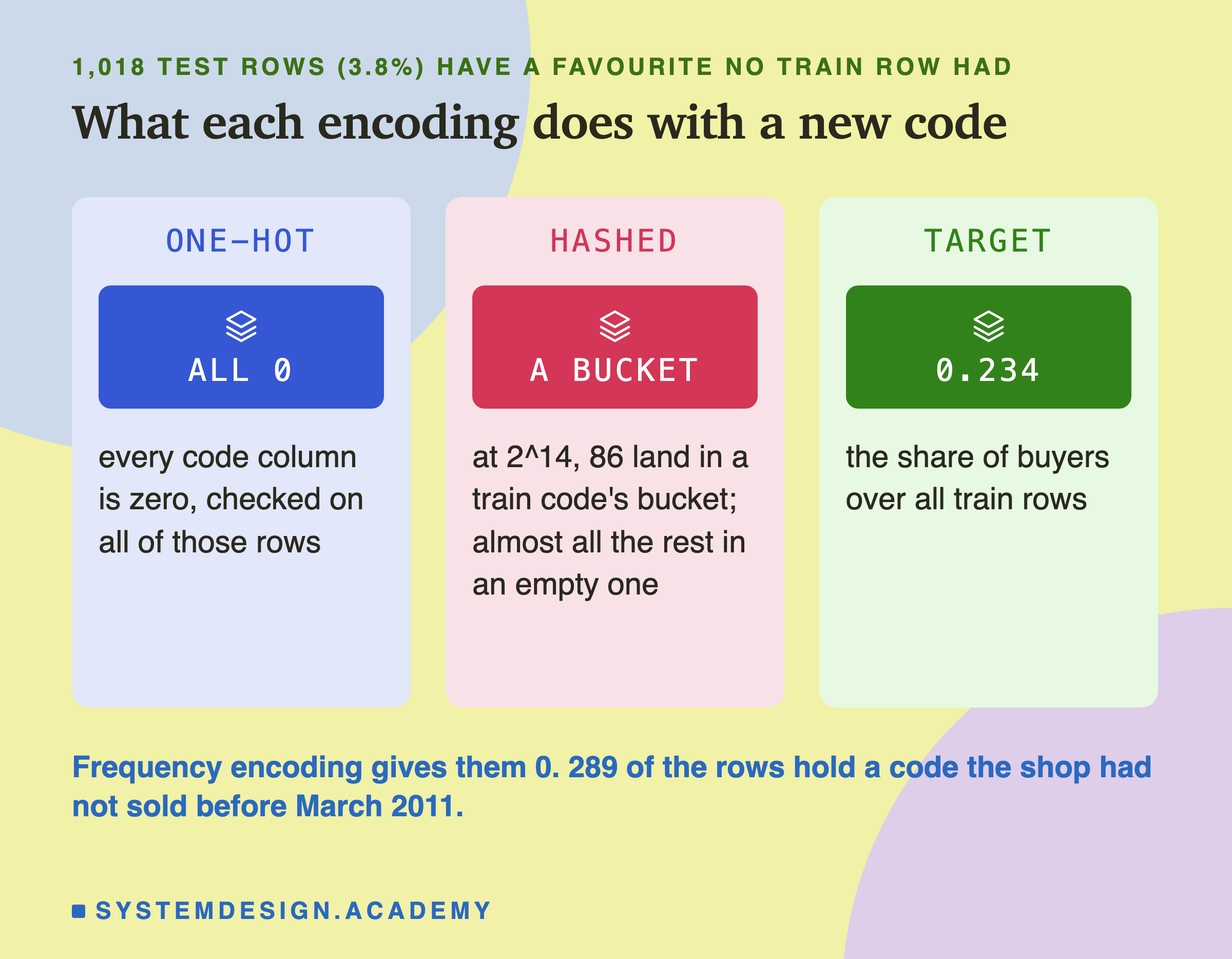
Each encoding has its own answer, and the lab checked each one on the real test matrices.
One-hot with handle_unknown="ignore" gives an unseen code a block of all zeros. The row then looks like a code the model never learned anything about.
Hashing has no idea what "unseen" means. The code lands in a bucket like any other. At 64 and 256 buckets, all 1,018 rows landed in a bucket a train code used, so they borrowed some other code's meaning. At 16,384 buckets only 86 did. Of the other 932, almost all landed in an empty bucket, which the model ignores; 8 landed in a bucket a country name uses.
Target encoding gives an unseen code the overall share of buyers in training, 0.234. That is scikit-learn's documented rule: the value is called target_mean_.
Frequency gives it 0, the share of train rows that hold it.
These rows matter more than their number suggests. 26.4 percent of them bought, against 19.5 percent of the other test rows. One possible reason, which I did not check: a customer whose favourite is new may be a customer who is buying a lot right now.
How the Encodings Did on New Codes
I scored the 1,018 unseen rows on their own. They are spread over the five test months, from 133 rows in July to 294 in November, so each month's AP rests on few buyers. Treat these numbers as rough.
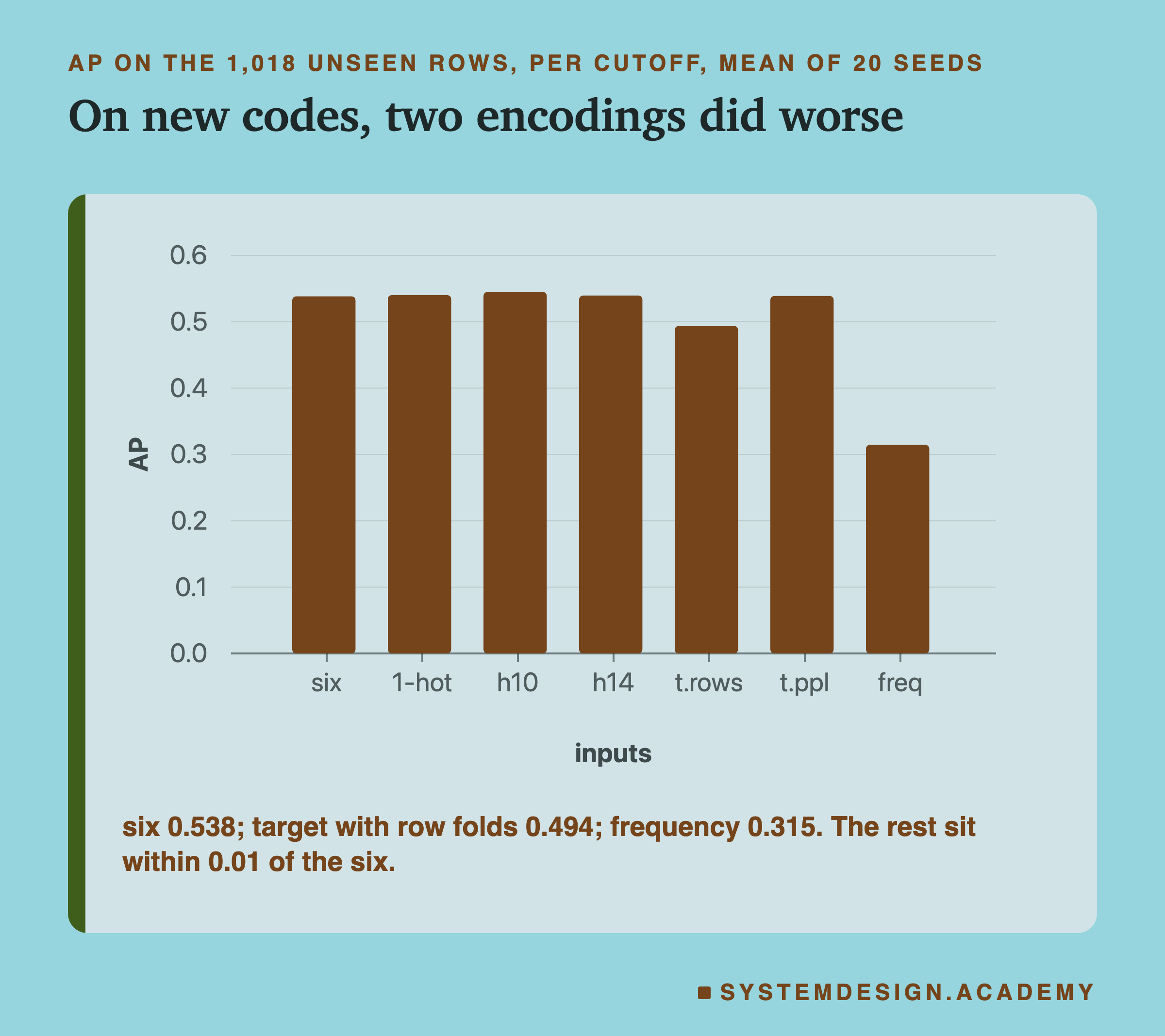
On these rows the six alone scored 0.538. One-hot scored 0.540 and hashing into 1,024 buckets 0.545. Their bootstrap intervals against the six, -0.0031 to +0.0071 and -0.0034 to +0.0177, both cross zero. So for new codes, giving them all zeros or a random bucket made no difference I could detect.
Two encodings did clearly worse here. Target encoding on folds of rows scored 0.494, an interval of -0.0751 to -0.0156. Frequency scored 0.315, an interval of -0.2696 to -0.1619.
Why would they do worse on new codes? Both give every new code one fixed value: 0.234 for target encoding, 0 for frequency. For frequency, a 0 never appears in training, so the model has never seen such a row. The next slides show that both encodings also learned something misleading in training.
Target Encoding: Folds of Rows Were Not Enough
Target encoding with the usual folds lost 0.0064. That was the first surprise, because those folds exist to stop a row seeing its own label. They did stop that. They did not stop something else.
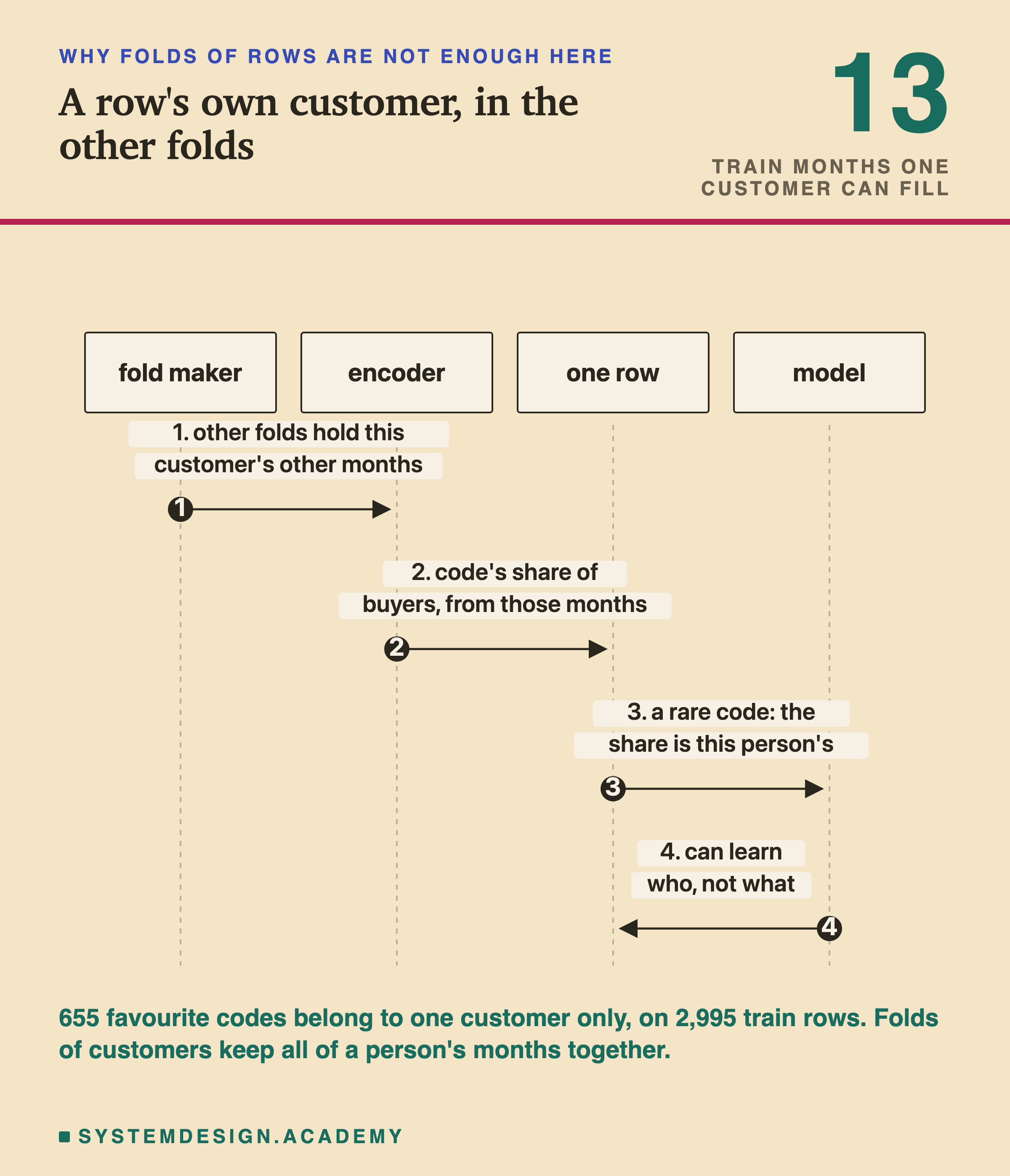
In this chapter, one customer appears once per month. One customer can fill up to 13 train rows. Folds of rows put those rows in different folds at random. So when a row's code is encoded "from the other folds", the other folds hold the same customer's other months, with their labels.
For a popular code that hardly matters. But 655 favourite codes belong to a single customer, on 2,995 train rows. For those, "the share of buyers with this code" is simply "how often THIS customer bought in their other months", some of them later months. That number knows about the customer's future.
So I had declared, before the run, a second version: the same encoder with folds of customers. All of one person's rows go into one fold, so a row is never encoded from its own person's labels.
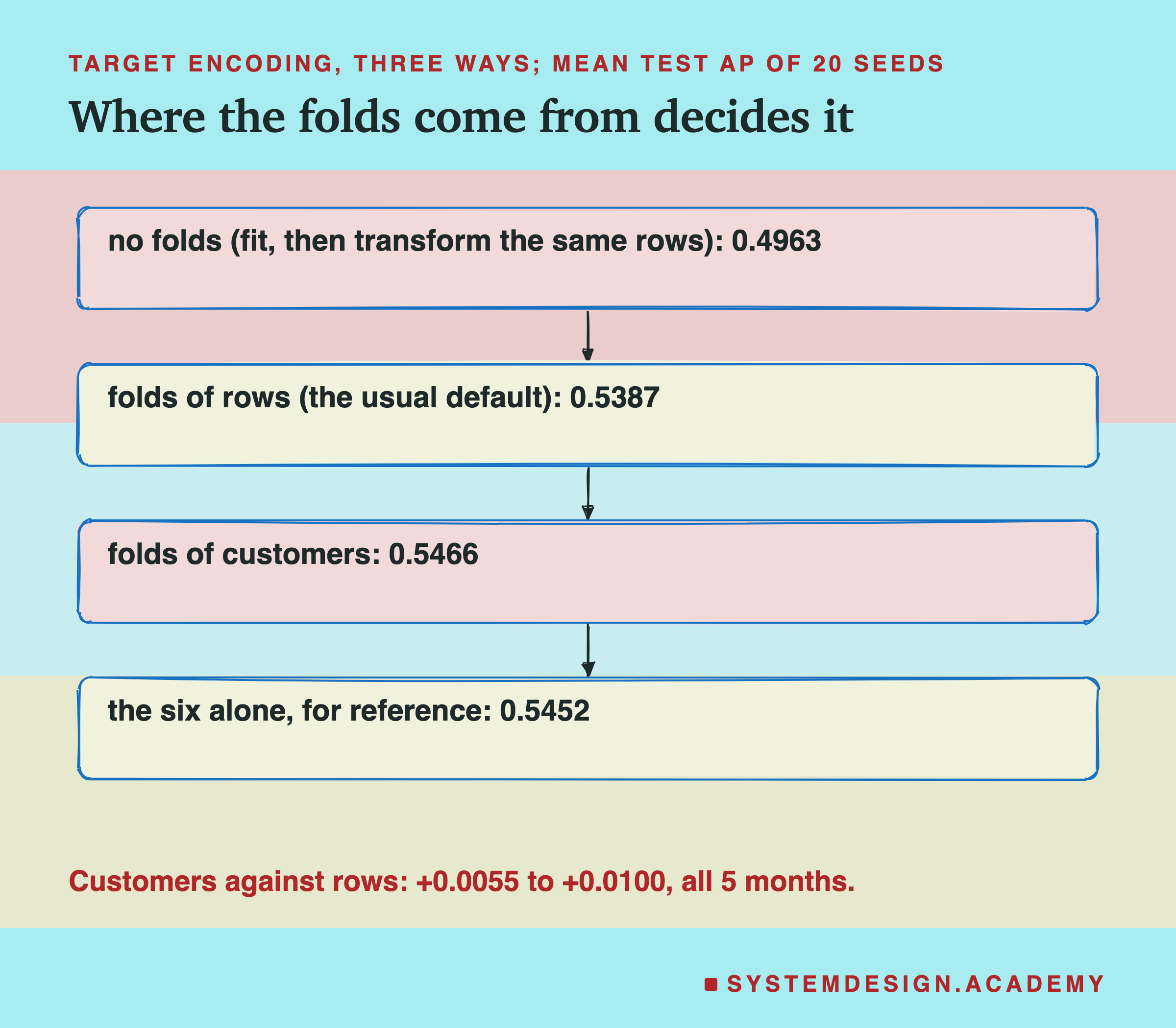
Folds of customers scored 0.5466, against 0.5387 for folds of rows. The interval for that difference was +0.0055 to +0.0100, and folds of customers won all 5 test months. The two contestants differ only in their folds, so the folds are what made the difference here. Against the six, folds of customers could not be told apart: -0.0003 to +0.0030.
With no folds at all, fitting the encoder and then transforming the same train rows, the score fell to 0.4963. The data engineering lesson on leakage before the split measured this leak on noise, so I will not repeat it here. scikit-learn's documentation warns about it directly: does not equal , because only cross-fits.
Choosing the Smoothing
Target encoding needs one more choice: smoothing. A code with only two rows has a share of buyers that is mostly luck. Smoothing pulls such a share toward the overall share. A bigger smoothing number pulls harder. scikit-learn also offers "auto", which picks the amount from the data.
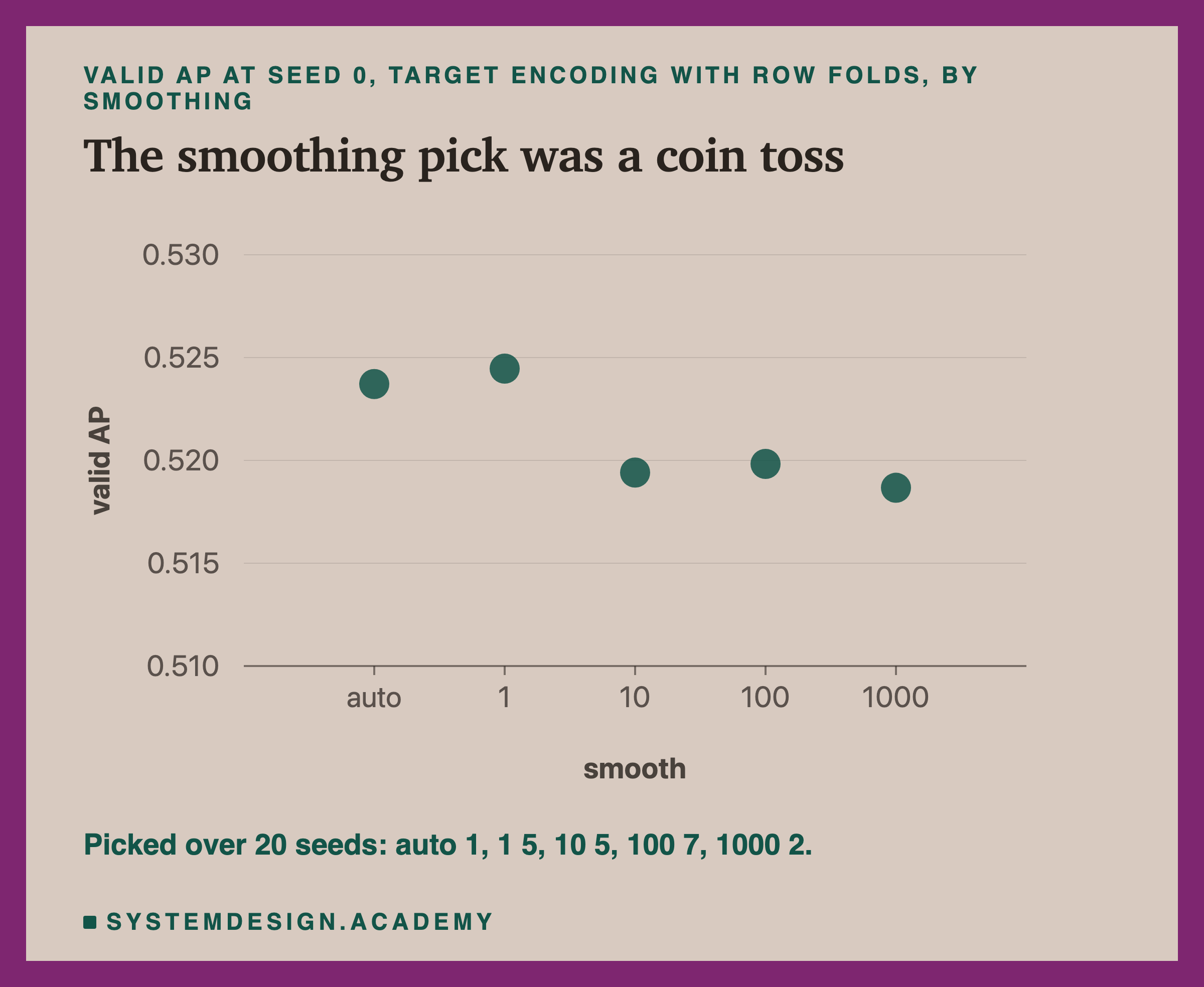
The design said to choose the smoothing on the valid months, at seed 0, using target encoding with folds of rows. Smoothing 1 won there with a valid AP of 0.5245, just above "auto" at 0.5237. All three target encoding contestants then used smoothing 1.
Then I looked at the other 19 seeds. The valid months picked "auto" once, 1 five times, 10 five times, 100 seven times and 1000 twice. So the choice was close to a coin toss. The valid scores of the five settings were all within about 0.006 of each other, and the random part of training was enough to change the order.
A confound to name: smoothing 1 is weak smoothing, so it leaves rare codes close to their own customer's buy rate. That may have made the folds-of-rows problem worse than a stronger smoothing would. I chose it by the rule written in advance and did not rerun with another.
The same thing happened with the hash size. At seed 0 the valid months picked 4,096 buckets. On the mean of all 20 seeds they picked 1,024. Both gave nearly the same test AP, 0.5474 and 0.5475.
Why Frequency Lost: Two Checks After the Results
Frequency encoding lost 0.1074, and it never reads the label. That made no sense to me at first. Everything on this slide was designed after I had seen the main results, and each check's design was written into the lab's docstring before it ran.
The first idea was wrong. I guessed the model was memorising customers, and that its early stopping could not see it, because early stopping holds out random rows and the same customers sit in those rows. So I trained again with early stopping on held-out CUSTOMERS instead: 10 percent of the train customers, none of whom the model trained on.
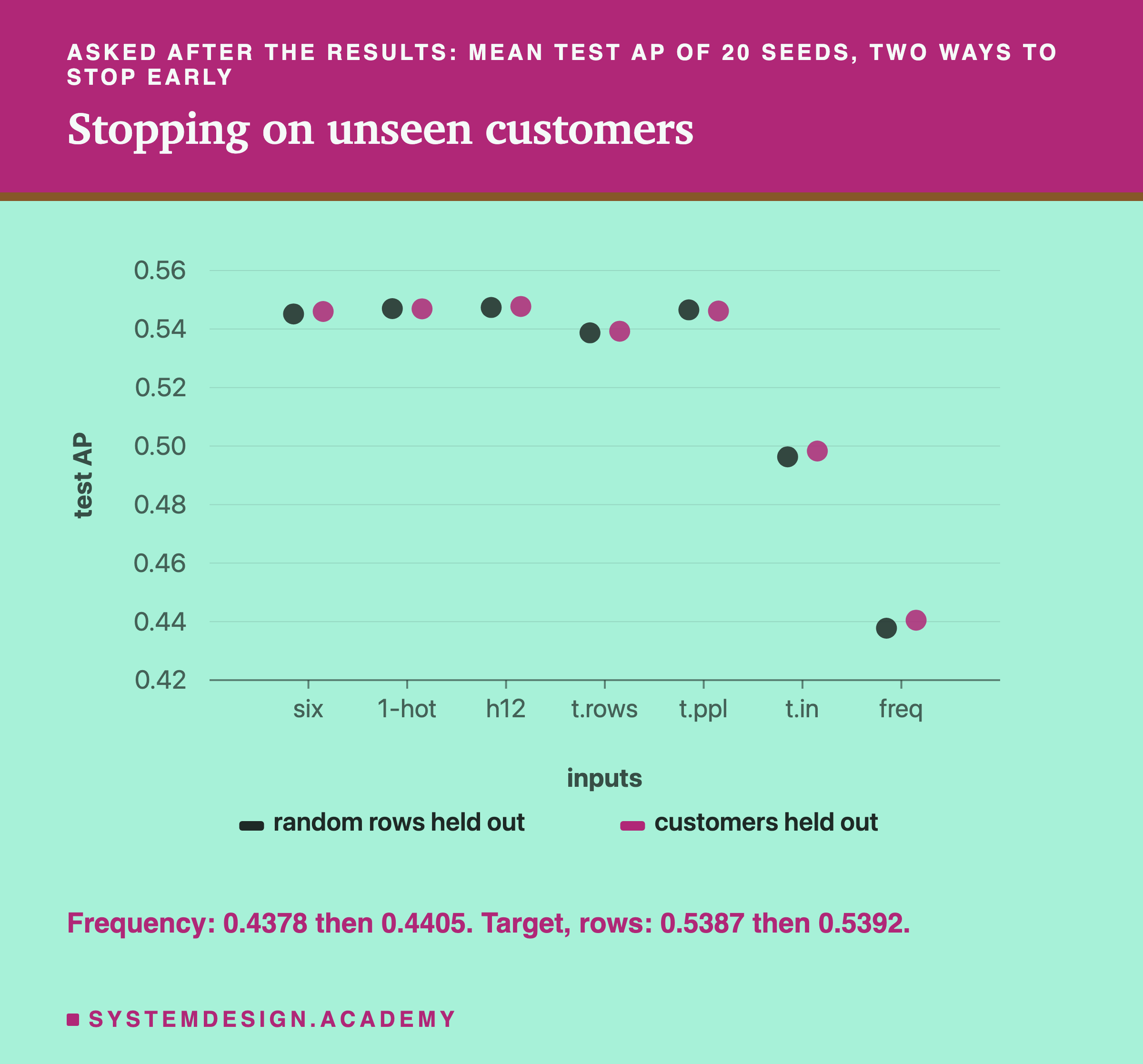
It changed almost nothing. Frequency went from 0.4378 to 0.4405, and target encoding on folds of rows from 0.5387 to 0.5392. So the way early stopping picked its rows was not the cause. This check did shake one result, though: one-hot's interval against the six became -0.0006 to +0.0024, which crosses zero, while 4,096 buckets stayed above it, +0.0003 to +0.0031. I would not lean on the one-hot gain.
The second idea fits the data, but it is not proved. The frequency of a code was counted over the rows of all 13 train months. So a row from March 2010 got a number that included rows from later months. Think about a code only one customer favours. A favourite only changes when the customer buys something. If they buy nothing new, the same favourite sits there month after month, and its count keeps growing. So a big count partly means "this person went on not buying". That is a fact about the future, hidden inside a plain count.
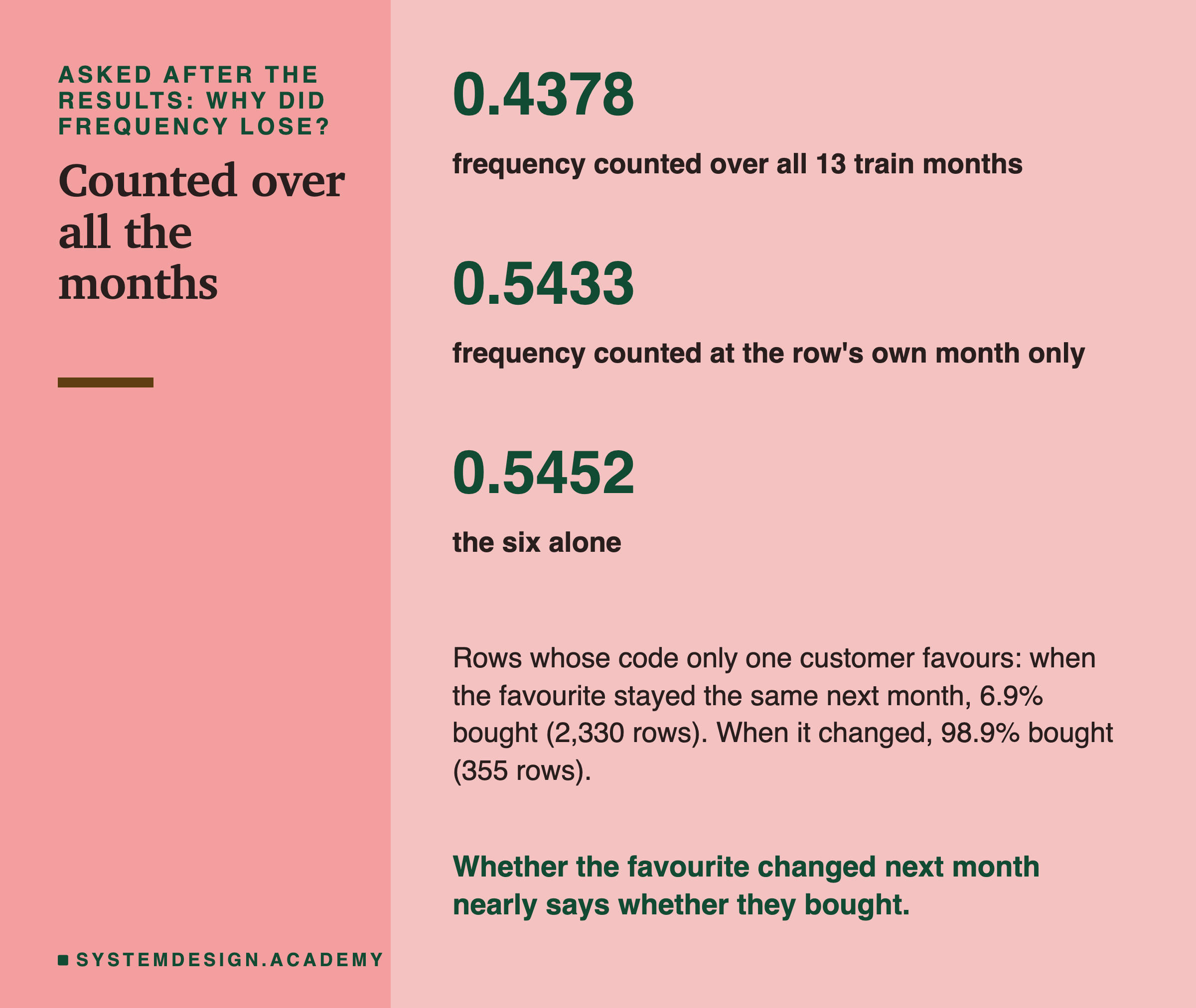
To test it, I counted frequency at each row's own month only: the share of that month's rows holding the code. It reads nothing after the cutoff, and a live system could compute it on the day. It scored 0.5433. Against the six, -0.0048 to +0.0011: the big loss was gone.
The Lab's Code, Piece by Piece
The lab is one file, scripts/labs/features/categorical_scale.py. It imports lesson 1's feature code for the six, so they are built exactly as before. Its base contestant must reproduce lesson 1's score of 0.5450 at seed 0, to twelve decimal places, or the run stops. It did.
favourites builds the column. For each cutoff it takes the events before the cutoff with one searchsorted, keeps the purchase lines, and counts lines per customer and code with groupby. It sorts by count, then by the latest time, then by the code, and keeps the first row per customer. The same pass builds each customer's bag as a sorted tuple of codes.
encode_unsupervised builds every contestant that does not read the label: OneHotEncoder(handle_unknown="ignore"), FeatureHasher(n_features=2**k, input_type="string", alternate_sign=False), and the frequency map. I turned off the hasher's alternating sign, which is on by default, so that a bucket is a plain count and two codes in one bucket really do look the same. The hasher gets the tokens "code=16156S" and "country=Italy" in one shared space, so a code can even collide with a country.
with_six stacks the six onto the encoded columns. For sparse encoders it first records the sparse table's bytes, then drops columns that are zero in every train row, then builds the dense table and records its bytes.
handles the three target versions. Folds of rows use . Folds of customers use with the customer id as the group. Since scikit-learn 1.9, accepts such a splitter as its . The no-folds version calls and then on the same rows.
Try It Yourself
The full lab trains several hundred models. I wrote a small demo that does the heart of it: it builds each customer's favourite code, then trains four models at seed 0 and prints their test AP.
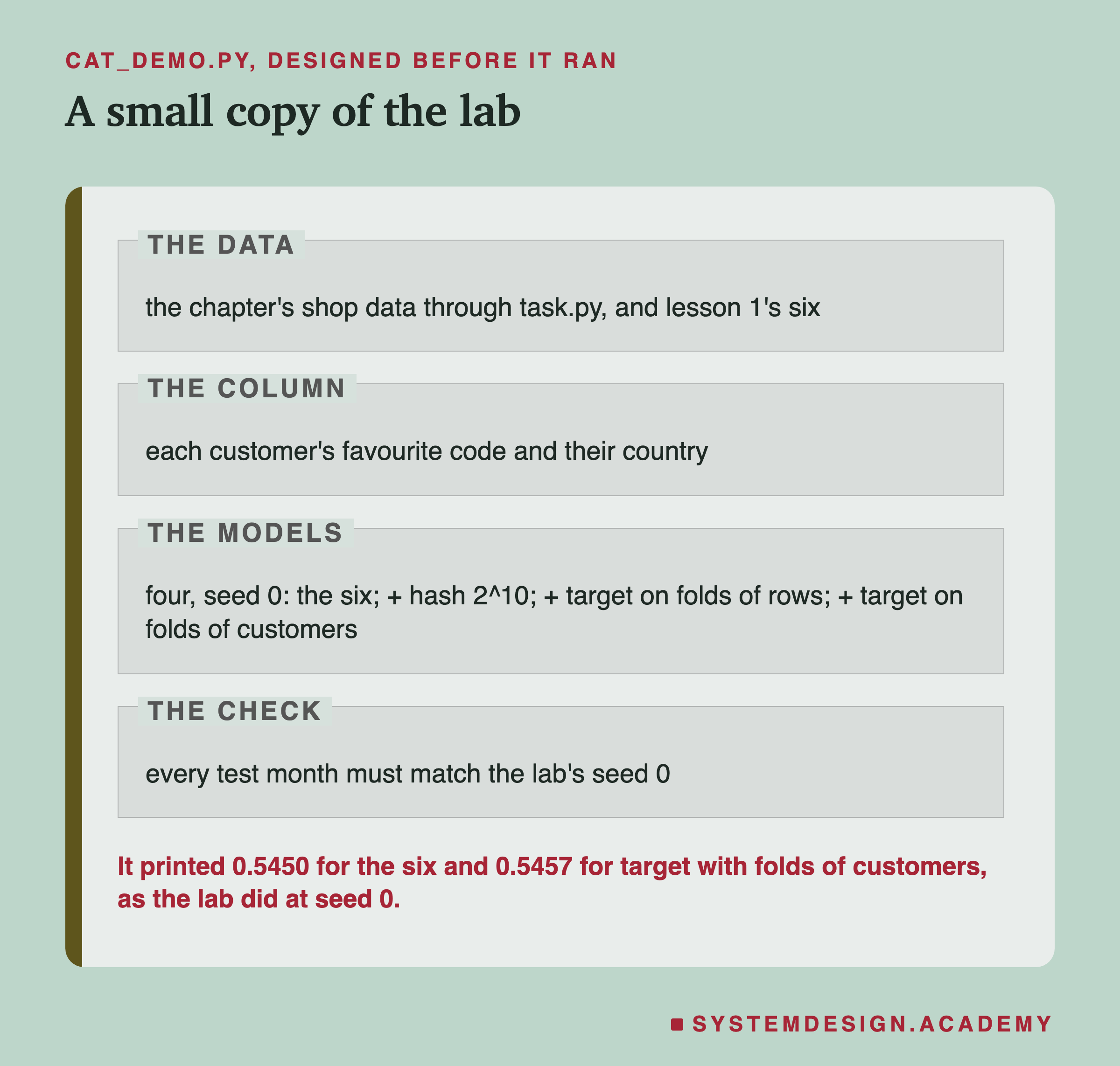
I wrote the demo's design into its docstring after the lab had run and before the demo first ran. My first version also trained the one-hot model. It was the slowest part by far, so I took that model out; hashing shows the same wide shape.
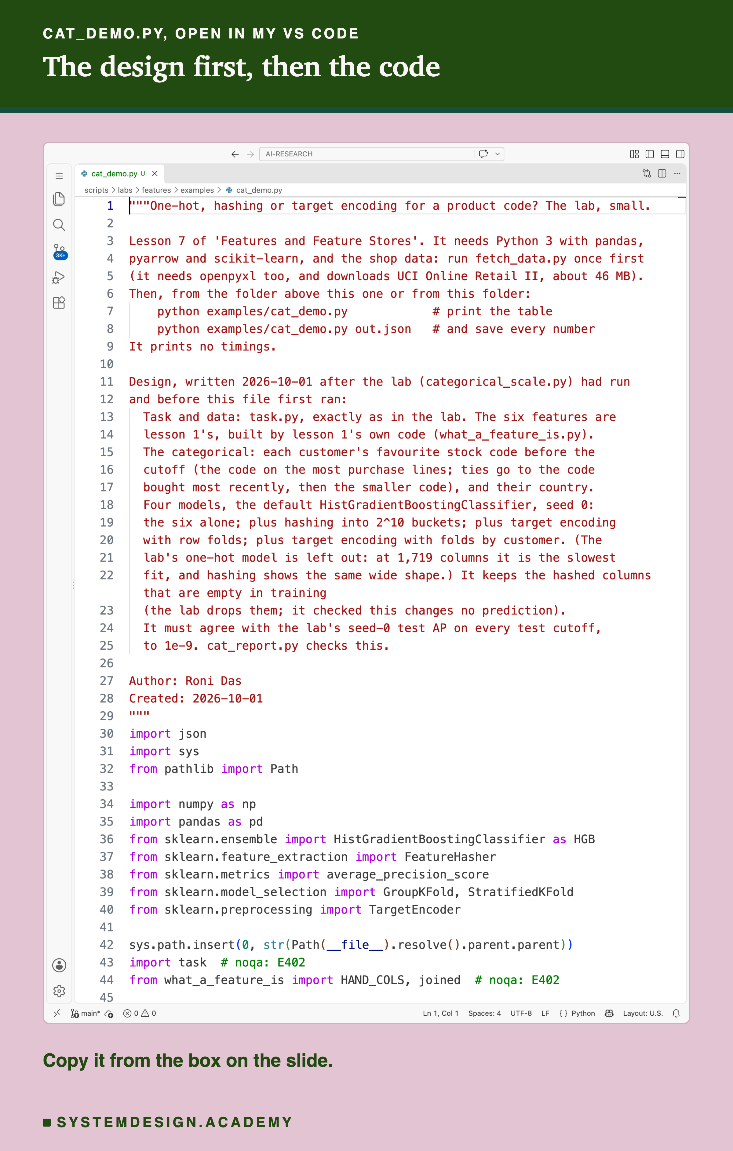
Before you run this lab. You need Python 3 with pandas, pyarrow and scikit-learn: pip install pandas pyarrow scikit-learn openpyxl. Use scikit-learn 1.9 or newer, because the demo hands TargetEncoder a list of folds. First run python fetch_data.py from the scripts/labs/features folder. It downloads the shop data once, about 46 MB, and writes one cleaned file. Then run the demo. It needs no GPU, and it should take about one to three minutes on a laptop. I ran it with scikit-learn 1.9.1 and pandas 3.0.6 on a Mac. These libraries run on Windows and Linux too, but I have not checked the numbers there. Give it a file name, python cat_demo.py out.json, and it also saves every number. That is how results/cat-demo.json was made.
"""One-hot, hashing or target encoding for a product code? The lab, small.

Lesson 7 of 'Features and Feature Stores'. It needs Python 3 with pandas,
pyarrow and scikit-learn, and the shop data: run fetch_data.py once first
(it needs openpyxl too, and downloads UCI Online Retail II, about 46 MB).
Then, from the folder above this one or from this folder:
    python examples/cat_demo.py            # print the table
    python examples/cat_demo.py out.json   # and save every number
It prints no timings.

Design, written 2026-10-01 after the lab (categorical_scale.py) had run
and before this file first ran:
  Task and data: task.py, exactly as in the lab. The six features are
  lesson 1's, built by lesson 1's own code (what_a_feature_is.py).
  The categorical: each customer's favourite stock code before the
  cutoff (the code on the most purchase lines; ties go to the code
  bought most recently, then the smaller code), and their country.
  Four models, the default HistGradientBoostingClassifier, seed 0:
  the six alone; plus hashing into 2^10 buckets; plus target encoding
  with row folds; plus target encoding with folds by customer. (The
  lab's one-hot model is left out: at 1,719 columns it is the slowest
  fit, and hashing shows the same wide shape.) It keeps the hashed columns that are empty in training
  (the lab drops them; it checked this changes no prediction).
  It must agree with the lab's seed-0 test AP on every test cutoff,
  to 1e-9. cat_report.py checks this.

Author: Roni Das
Created: 2026-10-01
"""
import json
import sys
from pathlib import Path

import numpy as np
import pandas as pd
from sklearn.ensemble import HistGradientBoostingClassifier as HGB
from sklearn.feature_extraction import FeatureHasher
from sklearn.metrics import average_precision_score
from sklearn.model_selection import GroupKFold, StratifiedKFold
from sklearn.preprocessing import TargetEncoder

sys.path.insert(0, str(Path(__file__).resolve().parent.parent))
import task  # noqa: E402
from what_a_feature_is import HAND_COLS, joined  # noqa: E402


def favourite(ev, lab, cutoffs):
    """Lesson 1's six, plus fav_code, per (customer, cutoff)."""
    d = joined(ev, lab, cutoffs)
    favs = []
    for t in cutoffs:
        buys = ev[(ev["ts"] < t) & ~ev["is_return"]]
        g = buys.groupby(["customer_id", "stock_code"])["ts"]
        c = g.agg(["size", "max"]).reset_index()
        c = c.sort_values(["customer_id", "size", "max", "stock_code"],
                          ascending=[True, False, False, True])
        f = c.drop_duplicates("customer_id")[["customer_id", "stock_code"]]
        favs.append(f.assign(cutoff=t))
    f = pd.concat(favs).rename(columns={"stock_code": "fav_code"})
    d = d.merge(f, on=["customer_id", "cutoff"], how="left")
    d["fav_code"] = d["fav_code"].fillna("none")
    return d


def test_ap(x_tr, y_tr, x_te, d_te):
    m = HGB(random_state=0).fit(x_tr, y_tr)
    p = m.predict_proba(x_te)[:, 1]
    d = d_te.assign(p=p)
    return [average_precision_score(g["label"], g["p"])
            for _, g in d.groupby("cutoff")]


ev = task.load_events()
lab_tr, _, lab_te = task.splits(ev)
tr = favourite(ev, lab_tr, task.TRAIN_CUTOFFS)
te = favourite(ev, lab_te, task.TEST_CUTOFFS)
y = tr["label"].to_numpy()
seen = set(tr["fav_code"])
unseen = int((~te["fav_code"].isin(seen)).sum())
print(f"rows: train {len(tr):,}, test {len(te):,}")
print(f"favourite codes in training: {len(seen):,}")
print(f"test rows with an unseen favourite: {unseen:,}")

cols = ["fav_code", "country"]
six_tr, six_te = (d[HAND_COLS].to_numpy(float) for d in (tr, te))
h = FeatureHasher(2**10, input_type="string", alternate_sign=False)
tok = lambda d: [[f"code={c}", f"country={k}"]  # noqa: E731
                 for c, k in zip(d["fav_code"], d["country"])]
bucket = {c: h.transform([[f"code={c}"]]).indices[0] for c in seen}
share = pd.Series(bucket).value_counts()
alone = sum(share[b] == 1 for b in bucket.values())
print(f"2^10 buckets: {len(seen) - alone:,} codes share a bucket")

arms = {"six alone": (six_tr, six_te)}
arms["+ hash 2^10"] = tuple(np.hstack([s, h.transform(tok(d)).toarray()])
                            for s, d in ((six_tr, tr), (six_te, te)))
folds = {"+ target, rows": StratifiedKFold(5, shuffle=True, random_state=0),
         "+ target, people": list(GroupKFold(5, shuffle=True, random_state=0)
                                  .split(tr, y, tr["customer_id"]))}
smooth = 1.0  # the lab picked this on the valid months, at seed 0
for name, cv in folds.items():
    enc = TargetEncoder(target_type="binary", smooth=smooth, cv=cv)
    e_tr = enc.fit_transform(tr[cols], y)
    arms[name] = (np.hstack([six_tr, e_tr]),
                  np.hstack([six_te, enc.transform(te[cols])]))

print(f"{'inputs':18s} {'columns':>7s} {'test AP':>8s}")
results = {}
for name, (x_tr, x_te) in arms.items():
    aps = test_ap(x_tr, y, x_te, te)
    results[name] = {"columns": x_tr.shape[1], "test": list(map(float, aps))}
    print(f"{name:18s} {x_tr.shape[1]:7d} {np.mean(aps):8.4f}")
if len(sys.argv) > 1:
    json.dump({"unseen": unseen, "fav_codes": len(seen),
               "shared_2_10": int(len(seen) - alone), "smooth": str(smooth),
               "arms": results}, open(sys.argv[1], "w"), indent=1)
Count the Collisions Yourself
This box holds the real 1,673 favourite codes from the train rows and how many train rows hold each. It also holds MurmurHash3, the hash scikit-learn's FeatureHasher uses, written in plain Python, so it runs in your browser. The report checked that it puts every code in the same bucket as scikit-learn, at all five sizes.
Press Run to see how many codes share a bucket at 1,024 buckets, how many train rows that touches, and what pure chance predicts. Then change BUCKETS to 2 ** 6 or 2 ** 14 and run again. Last, change MINE to any code in the list, and see which codes share its drawer.
At the bottom it also prints each contestant's real mean test AP over 20 seeds, so you can set the collisions next to what they cost, or did not cost, in score.
Common Mistakes, and When Each Choice Helps
Counting over the whole training table. Frequency encoding, target encoding and any other count of a name must use only rows from before each row's cutoff, or the count carries the future in. Here that cost 0.1074 in AP, on an encoding that never reads the label.
Folds of rows when one person has many rows. If the same customer, user or device appears in many rows, fold by that person. Here folds of rows lost 0.0064 and folds of customers did not.
Fitting and transforming the same rows. With scikit-learn's TargetEncoder, call fit_transform on the training rows, and pass cv= a split by person, such as GroupKFold by customer, because the default row folds lost 0.0064 here. Use transform on new rows. Never fit then transform on the training rows.
Trusting a big hash to have no collisions. Even 16,384 buckets for 1,673 codes left 173 codes sharing. Count them, it is cheap.
Forgetting the unseen rows. Score them on their own. Here they were 3.8 percent of rows, but they bought more often than the rest.
When hashing helps most. When names keep arriving, when memory is tight and the model can read sparse tables, and when a few collisions are an acceptable price. My guess, not tested here, is that it shines most with a linear model.
When one-hot is enough. When the names are few, or settled, or the model reads sparse tables, as a linear model does.
When target encoding helps. When there are many names, a tree model, and enough rows per name, and only with folds that respect both time and the person.
What This Lab Cannot Tell You
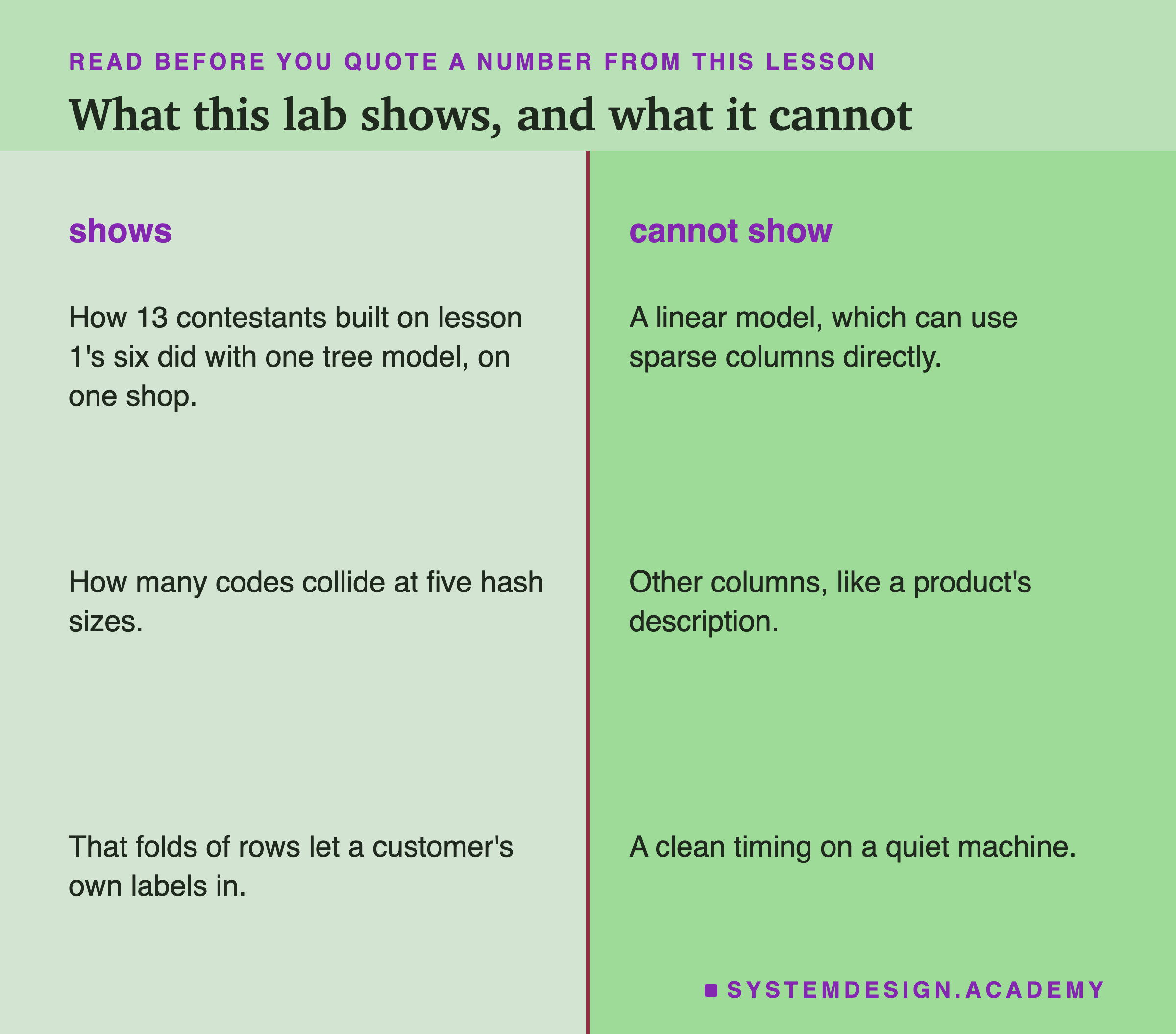
One shop, one task, one model. A tree model with default settings, on a 30-day buying question. A linear model reads sparse tables natively and weighs every column on its own; it might gain more from one-hot or hashing. I did not test one.
One choice of column. I encoded each customer's favourite code. A description of the product, the shop's own product groups, or the bag with a richer model could behave differently. A later lesson in this chapter is planned to look at descriptions.
Folds of customers are still not point-in-time. They keep a person's own labels out, but a row from March 2010 is still encoded using other customers' labels from later months. A strictly time-respecting target encoding would use only rows from before each cutoff. I did not build one.
Two checks were added after the results. Both are labelled on the frequency slide, and their designs were written down before they ran. The first one did not support my idea; the second did.
No timings. The laptop was busy with another lab, so I report column counts and bytes only.
What to Do on Monday
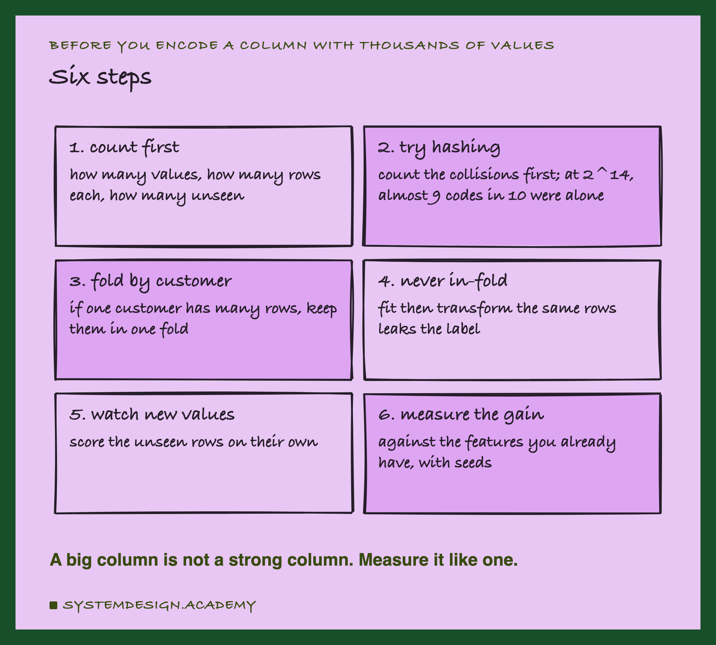
These are the steps I would take the next time someone hands me a column with thousands of names.
-
Count first. How many names, how many rows hold each, how many arrive after training. Here 655 codes belonged to one customer only. Had I looked at that first, it would have warned me about the target encoding result.
-
Try hashing, and count its collisions. It needs no fitting and has an answer for every new name. Pick the size on valid months.
-
Fold by the person, and stay before the cutoff. For any encoding that counts or reads labels.
-
Never fit and transform the same rows with a target encoder.
-
Score unseen rows on their own.
-
Measure the gain against the features you already have, with 20 seeds and an interval. Here the size picked on the valid months gained +0.0024.
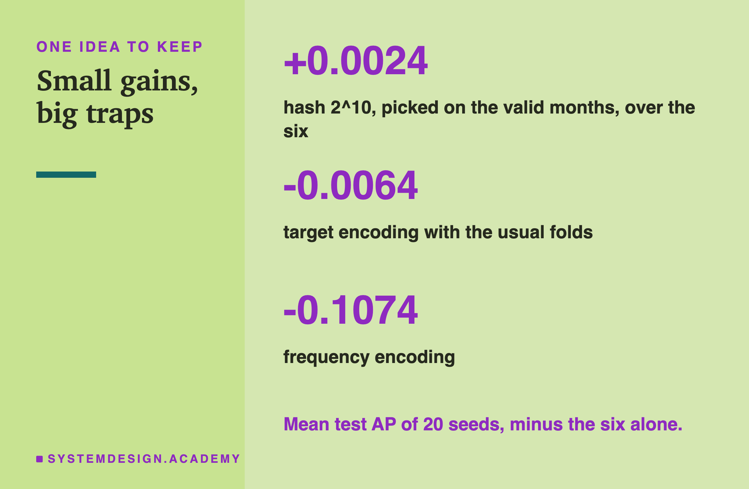
The one idea to keep: on this shop, the way a product column was encoded mattered less for what it could add than for what it could break. A plain count over the whole training table broke the model; one that stayed inside each month did not.
Knowledge Check
Knowledge Check
4 questions - Score 80% to pass
Frequency encoding never reads the label. Why did it still lose so much here?
Target encoding with folds of rows lost to the six, but folds of customers did not. What changed between them?
At 16,384 buckets there were almost ten buckets for every favourite code. What did the lab find?
One-hot needed 612.3 MB as a dense table but only 1.2 MB as a sparse one. Why the difference?