Imagine a small town that hires a weather forecaster. Every evening she studies the clouds, the wind and the pressure, and writes her forecast for tomorrow on a board in the square. She is proud of her record: she is right seven days out of ten.

Now imagine her neighbour, who knows nothing about weather. Every evening he writes the same thing on a card in his window: "Tomorrow will be like today." If it was dry today, he says dry. If it rained, he says rain. He never looks at a cloud. And because weather tends to last for a few days at a time, he is right more often than you would think. In some towns he would be right more often than she is.

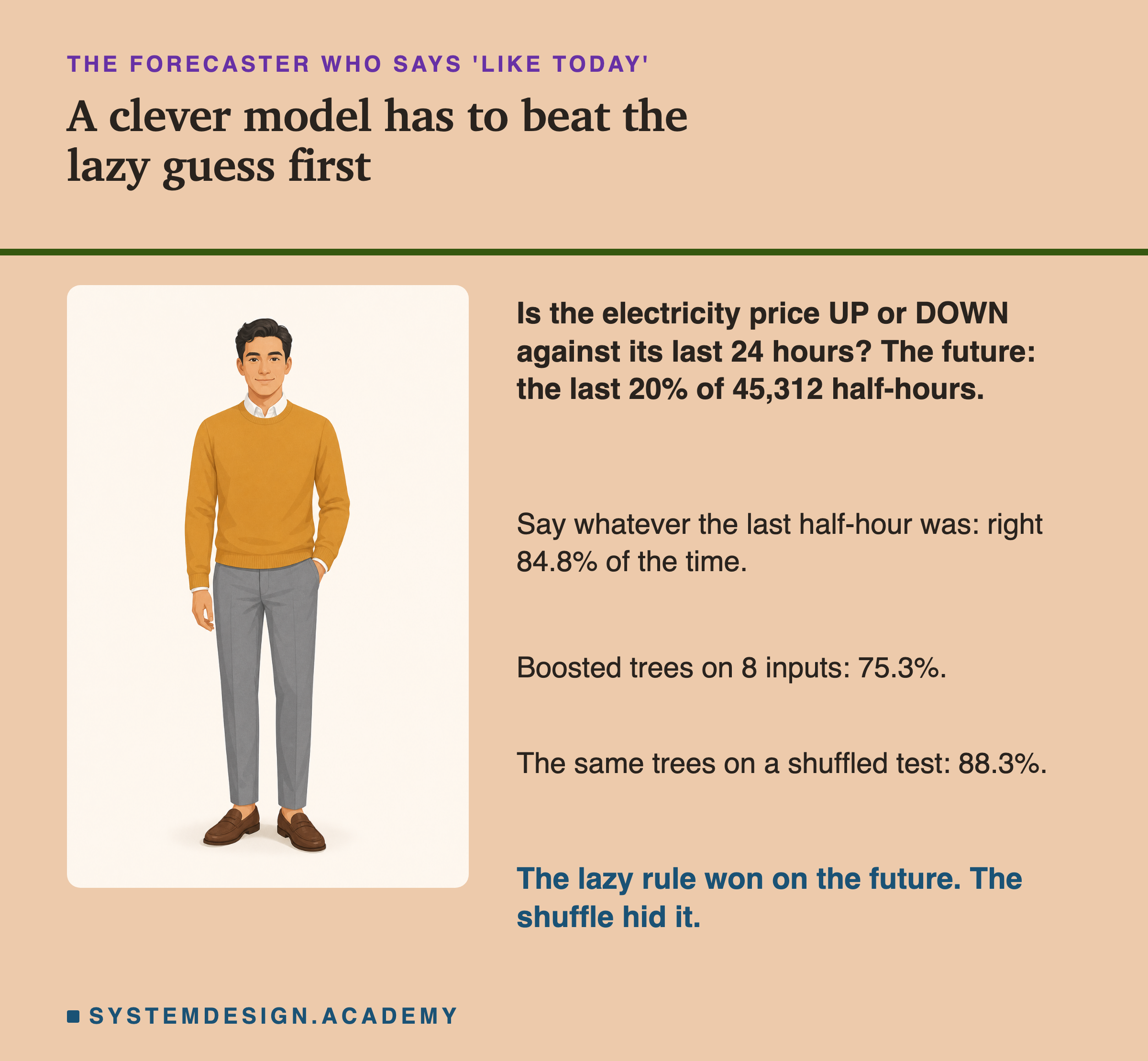
Her seven days out of ten sounds good on its own. It only means something next to his number. If he is right eight days out of ten, all her study has made the forecast worse, not better, and the town would do well to read his card.

This lesson does the same thing to programs that learn from examples. Before I trust a trained model's score, I score the laziest rules I can think of, on the same test, the same way. On the data in this lesson, the laziest rule of all won, and a shuffled test would have hidden that.

This is the first lesson of a new chapter, and the chapter is about the lifecycle of a model: all the steps between an idea and a model that has been in use for a year. You frame the problem, get the data, set baselines, train a model, evaluate it, ship it, watch it, and retrain it, and then the last steps repeat for as long as the model is used.

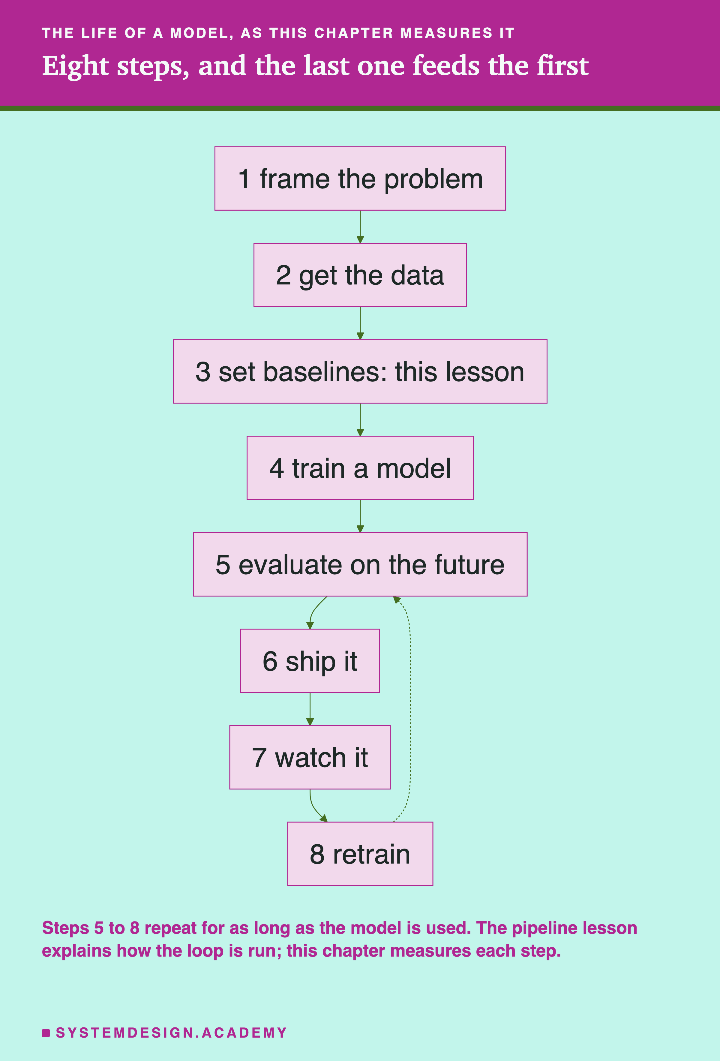
The course already has a lesson that explains how that loop is run by software: training pipelines and orchestration describes the graph of steps, what triggers a run, the gate a new model must pass, and how runs are tracked. I will not repeat it here. That lesson explains each step in words. This chapter measures each step on real data, one lesson at a time, and shows what goes wrong when a step is skipped.

The chapter before this one, Why Production Breaks, measured what goes wrong after a model ships. Its first lesson, the score that lied, showed that a test on rows picked at random can flatter a model (make it look better than it is) when the rows arrive in time order. This lesson builds on that without repeating it. It adds the step that comes before any trained model at all: the rules with no learning that the model has to beat.

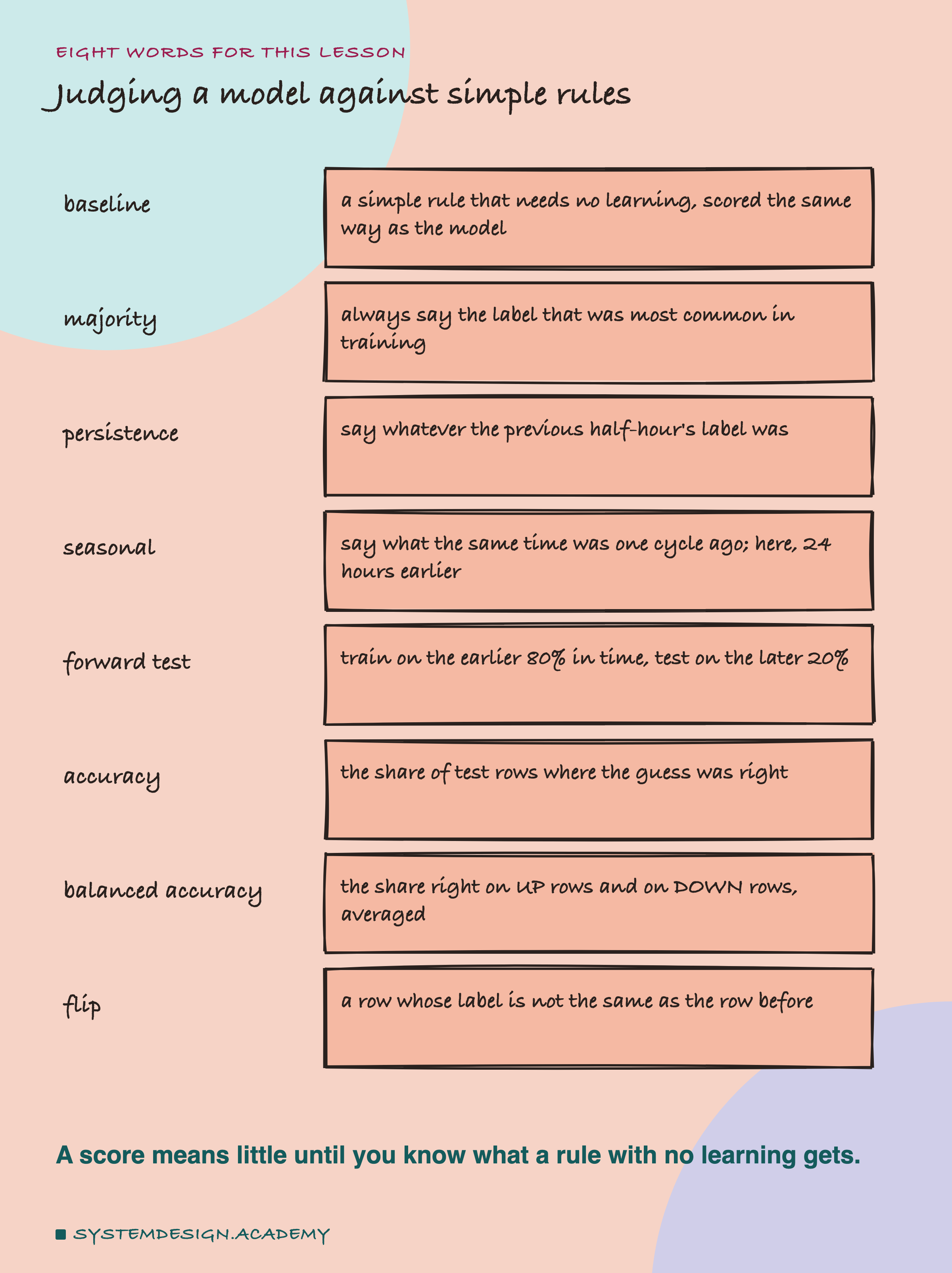
A model is a program that learned from examples. Here it learns to choose between two answers, UP or DOWN, which is called classification; the answer for one row is its label. A baseline is a simple rule that needs no learning at all, scored on the same test in the same way as the model. It is the number a model has to beat before its own number means anything.

Three baselines appear in this lesson. The majority rule always says the label that was most common in the training rows. The persistence rule says whatever the previous row's label was, like the neighbour's card. A seasonal rule says what the label was at the same point one cycle earlier; here the cycle is a day, so it says what the same half-hour was 24 hours before.

A forward test trains on the earlier 80% of the rows in time and tests on the later 20%, the future from the model's point of view. Accuracy is the share of test rows where the guess was right. Balanced accuracy is the share right on the UP rows and the share right on the DOWN rows, averaged, so both labels count equally. A flip is a row whose label is not the same as the row before it.

Two steps come before any training, and this lesson touches both.

Framing means writing down exactly what the model must guess, when it must guess it, and what is already known at that moment. It sounds like paperwork. It decides which baselines are fair. The persistence rule uses the previous half-hour's label. That is only allowed if the previous label is known when the next guess is made. Here it is: the label for one half-hour depends only on prices up to that half-hour, so it is known once that half-hour's price is known, before the next guess. If your labels arrive a week late, persistence has to use the last label you would really have, which is a weaker rule, and you should score that version instead.

Baselines come next, before any model is trained, and for a plain reason: a trained model's score has no scale of its own. An accuracy of 0.75 is excellent if the laziest rule gets 0.55 and it is a loss if the laziest rule gets 0.85. The same number can mean progress or damage, and only a baseline says which.

So the rule this lesson tests is simple. A model must beat the best trivial rule, on a forward test, before anything else is worth doing. Not the worst trivial rule, and not on a shuffled test. If it cannot, do not go on to step five: ship the rule, or go back and frame the problem again.

Why the best rule and not just any rule? Because the easy baseline to beat is usually the majority rule, and a model that beats only that one tells a reader very little. For data in time order, persistence or a seasonal rule may be much stronger, as they were here, so they have to be scored too.

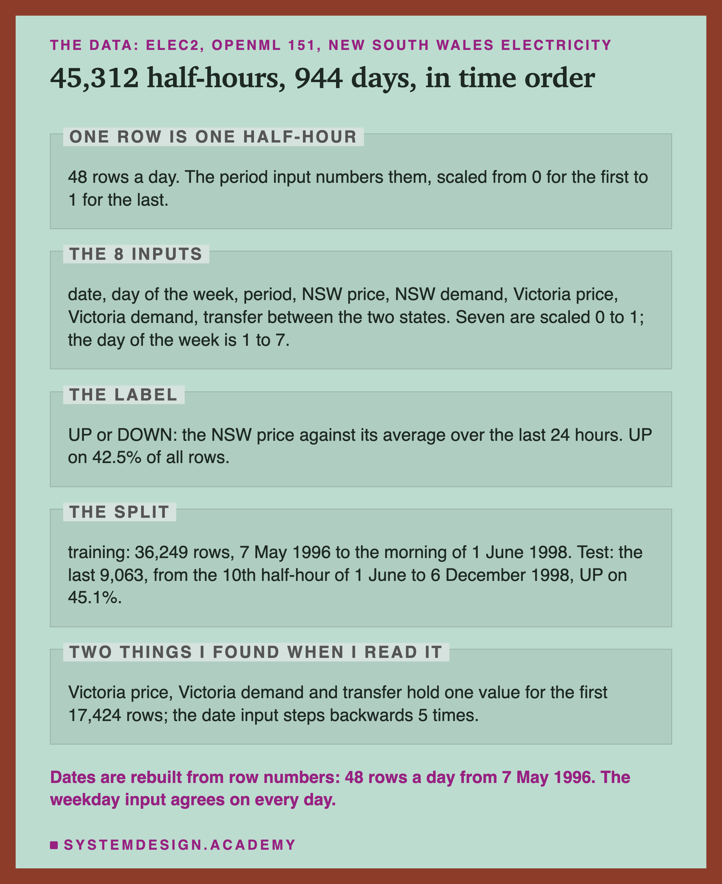
The data is Elec2, a public dataset from the electricity market of New South Wales (NSW), a state of Australia. I use the copy on OpenML, a free public website that stores datasets for machine learning (dataset 151, version 1, listed with a public licence), because scikit-learn, the free Python library I use for every model in this chapter, can download it with one call. It is a benchmark: a public dataset that many people have used to test their methods, so results can be compared. It has 45,312 rows. Each row is one half-hour, and the rows are in time order: 48 rows a day for 944 days. In this market the price is not fixed; OpenML's description says prices are set every five minutes and move with demand and supply.

Each row has eight inputs: a date, the day of the week, the period (which half-hour of the day it is), the NSW price and demand, the price and demand in the neighbouring state of Victoria, and the planned transfer of electricity between the two states. Seven of them are scaled to lie between 0 and 1; the day of the week runs from 1 to 7. The label, class, is UP or DOWN. UP is the rarer label: 42.5% of all rows.

I read the data before I wrote anything about it, and two things came out that matter. First, three columns, the Victoria price, the Victoria demand and the transfer between the states, hold a single value for the first 17,424 rows, about the first year; the dataset's description does not say why, so I will not guess. Second, the date input is not a clean calendar: it stays the same within each day but steps backwards between days 5 times. So I rebuilt the dates from the row numbers instead: 48 rows a day, starting on 7 May 1996, the first day OpenML gives. The day-of-week input agrees with that calendar on all 944 days. The rebuilt last day is 6 December 1998; OpenML's description says 5 December, so one of the two is a day out, and I cannot tell which from the file.

The label is the most important column, so I checked what it really is. OpenML's description says, word for word: "The class label identifies the change of the price (UP or DOWN) in New South Wales relative to a moving average of the last 24 hours (and removes the impact of longer term price trends)."

A moving average of the last 24 hours is the average of the previous 48 half-hourly prices, recomputed at every row. So I computed it and compared. On every one of the 45,264 rows that have 48 earlier rows, the label is UP exactly when the NSW price is above the average of the previous 48 prices, and DOWN otherwise. That held on all 45,264 of them, with no exception. On the first 47 rows, where fewer than 48 earlier prices exist, a shorter average matched 41 times, so the dataset's authors handled the start in some way I could not reproduce. This check is mine, done after the results.

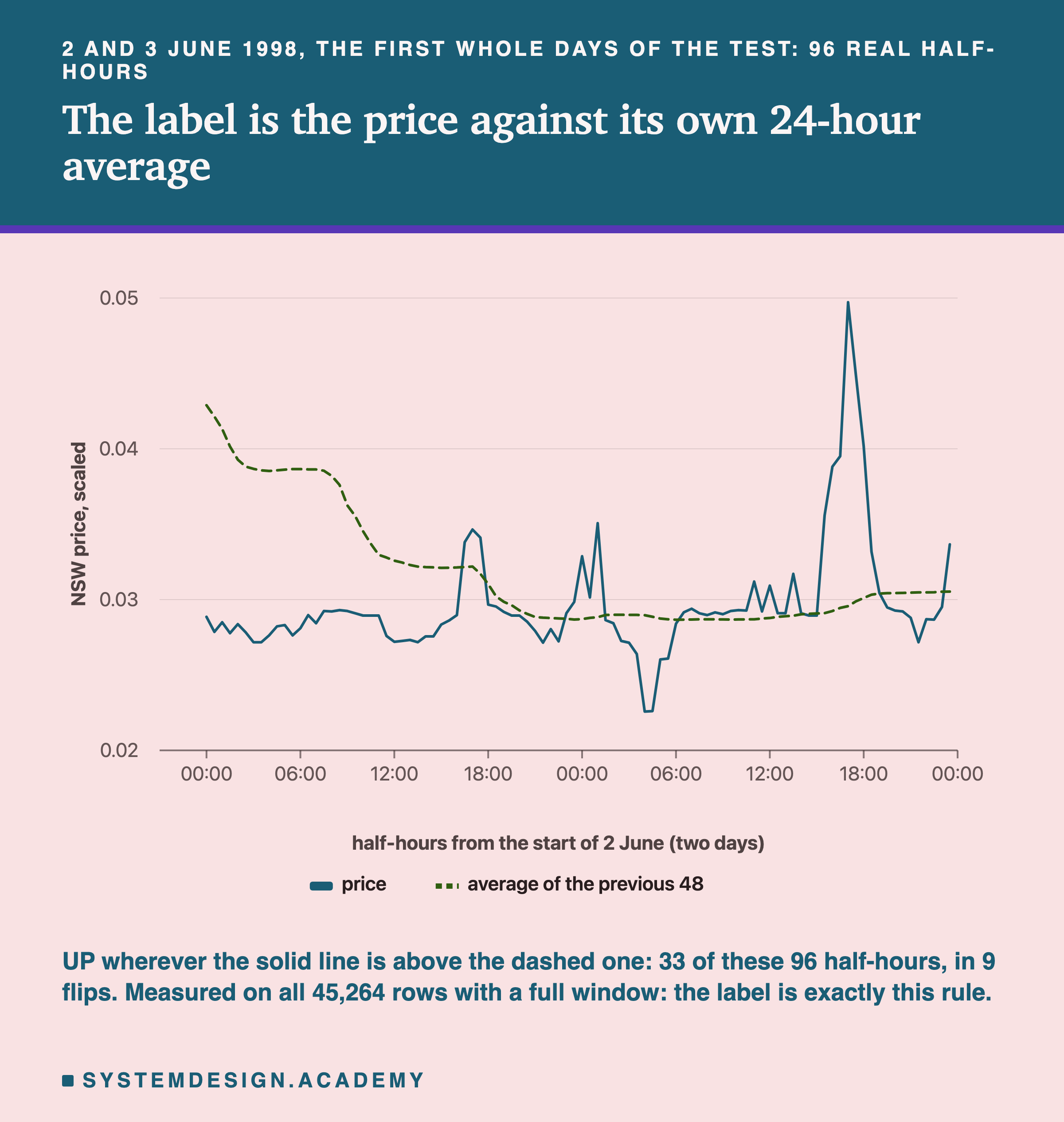
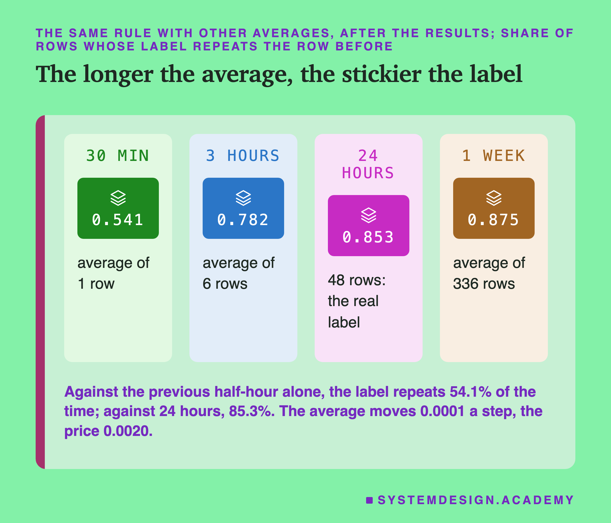
That has a consequence the rest of the lesson keeps meeting: the label is sticky by construction. The average of 48 prices moves slowly, because each new row changes only one of the 48. Over the whole data, the median (the middle value, if you line them all up) step of the average from one row to the next was 0.0001, while the median step of the price itself was 0.0020, and the median distance between the price and its average was 0.0085. So the price usually sits well on one side of a slow line, and it takes a real move to cross it.

Here are the three baselines, one at a time.

Majority looks at the training rows once, finds the most common label, and says it for every test row. In training, DOWN was more common, so it says DOWN 9,063 times. It is right on every DOWN row and wrong on every UP row.

Persistence says whatever the previous half-hour was. For the first test row it uses the last training row's label. It never looks at a price. It can only be wrong when the label changes, and on those rows, the flips, it is always wrong.

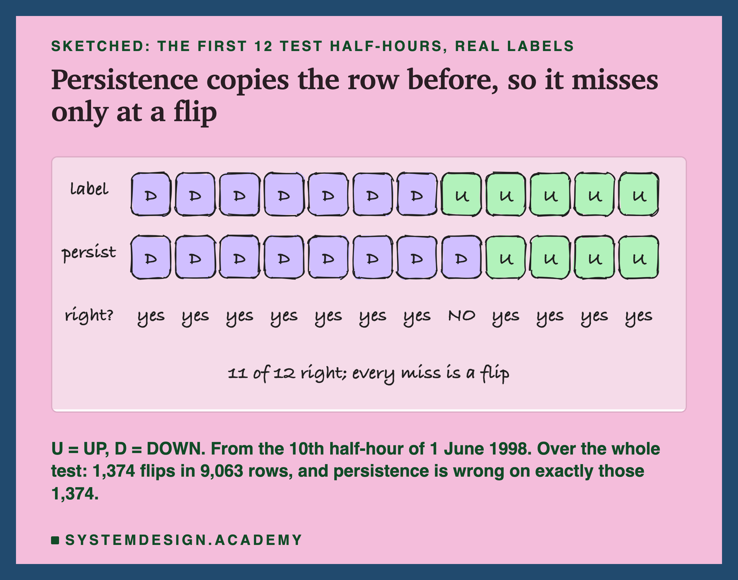
These are the first 12 test rows, with real labels. The label is DOWN seven times, then UP five times. Persistence copies each label one row late, so it misses once, at the eighth row, where the label flipped, and is right on the other 11.

Same period yesterday is the seasonal rule. It says the label of the same half-hour 24 hours earlier, 48 rows back. Electricity has a daily rhythm: demand rises in the morning and evening. If the label followed that rhythm closely, this rule would be strong.

None of these rules needs a library or a computer to learn anything. Each is one line of code. That is the point: if one of them beats your model, your model's extra work adds nothing, and the rule is cheaper to run, easier to explain and has no training data that can go stale.

I wrote the lab's design at the top of its file, baseline_lab.py, before I ran it: the question, the data, the split, the three rules, the three models and their settings, and the two scores. The dated record is in the chapter plan (2026-09-29, "BASELINE LAB (batch 1) designed before running").

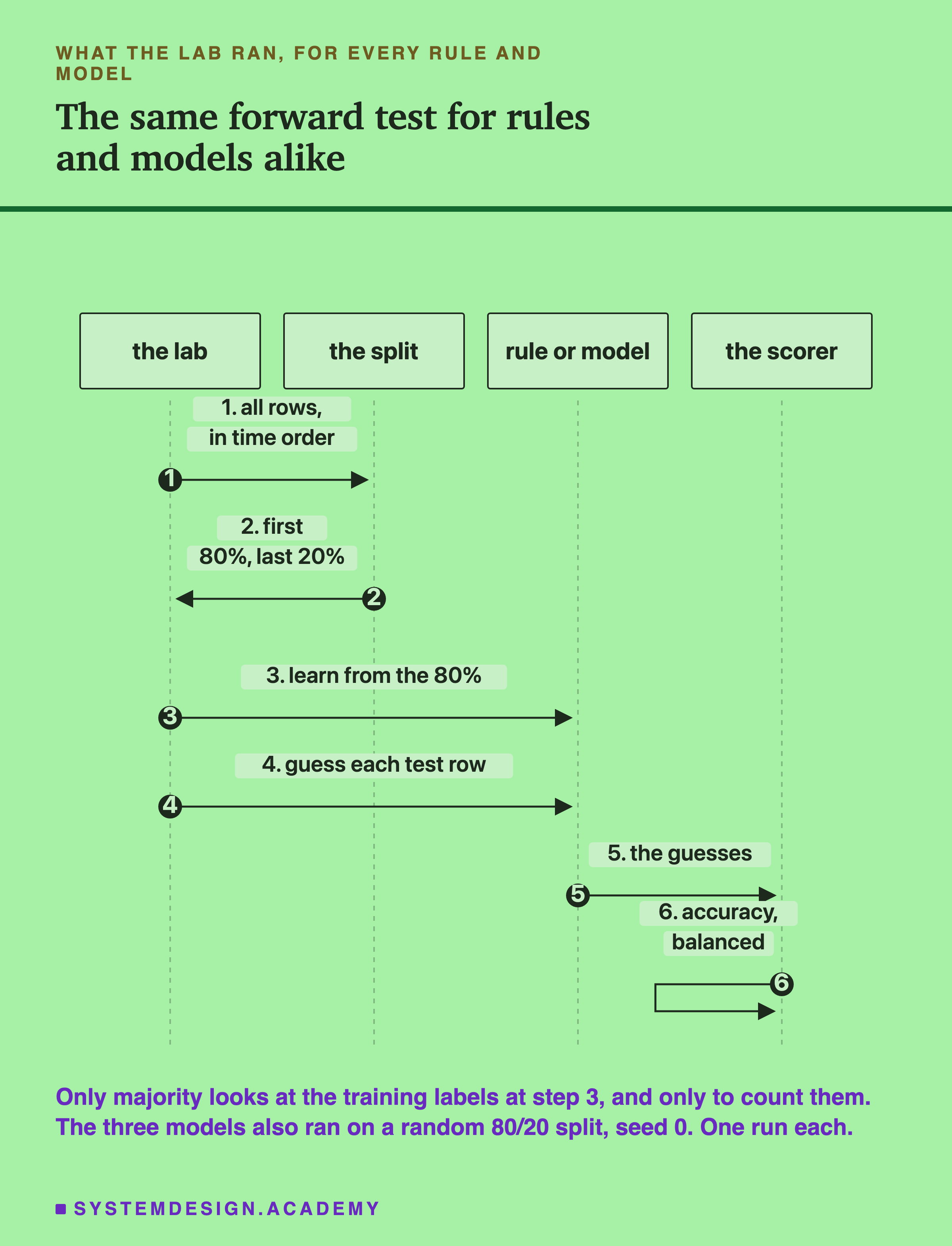
The three models. The first is logistic regression, which adds up a weight for each input and turns the sum into a choice between UP and DOWN; the inputs were first standardised: each one shifted and rescaled so that its average is 0 and its spread is 1. The second is scikit-learn's HistGradientBoostingClassifier, which I call boosted trees: many small trees of yes-or-no questions about the inputs, built one after another, each one correcting the errors of the ones before. The third is the same trees with one extra input: the previous half-hour's label. I call it trees plus lag, because an input that holds an earlier value of something is often called a lag. All three ran with scikit-learn's default settings, and the trees with random_state=0, a fixed seed for their own random choices. No tuning.

The split. Forward, as in the score that lied: the first 36,249 rows train, the last 9,063 test. The three models were also trained and scored on a random 80/20 split with seed 0, to see the gap between a shuffle and the future again on a new dataset.

Every rule and model ran once. A is a calculation that says how likely a gap this size would be by luck alone. None was declared before the run, so I will not call any gap significant. Every number below comes from the lab's stored file, .

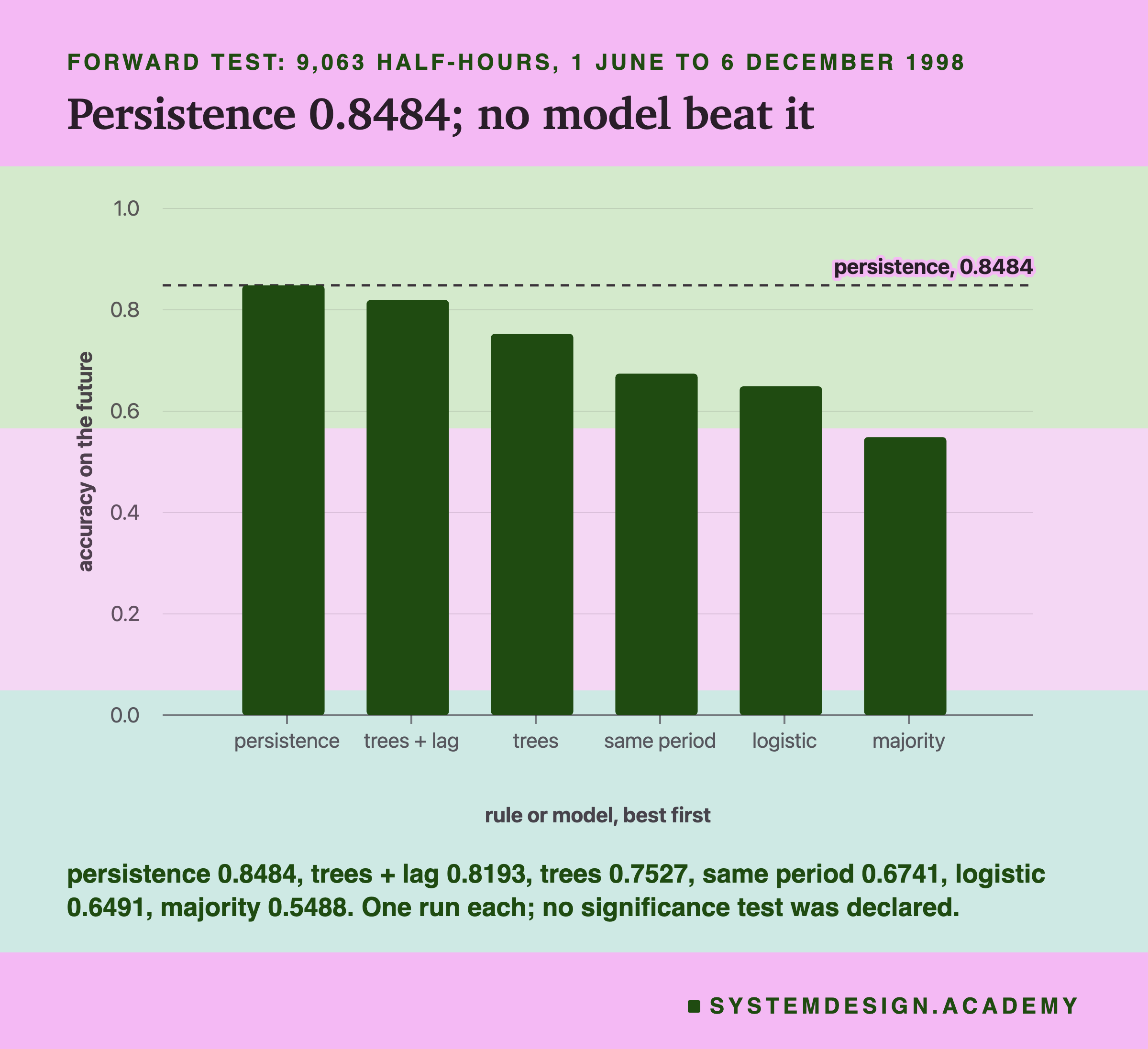
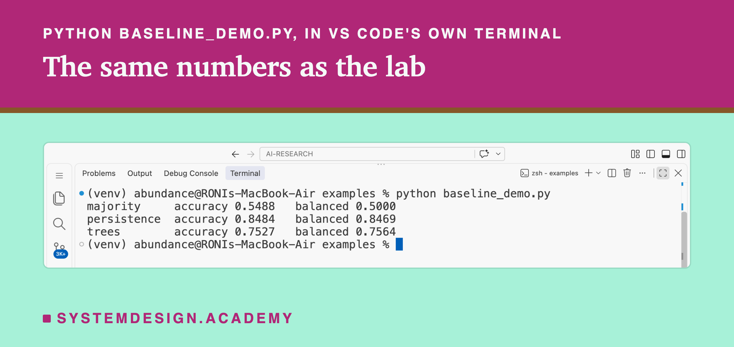
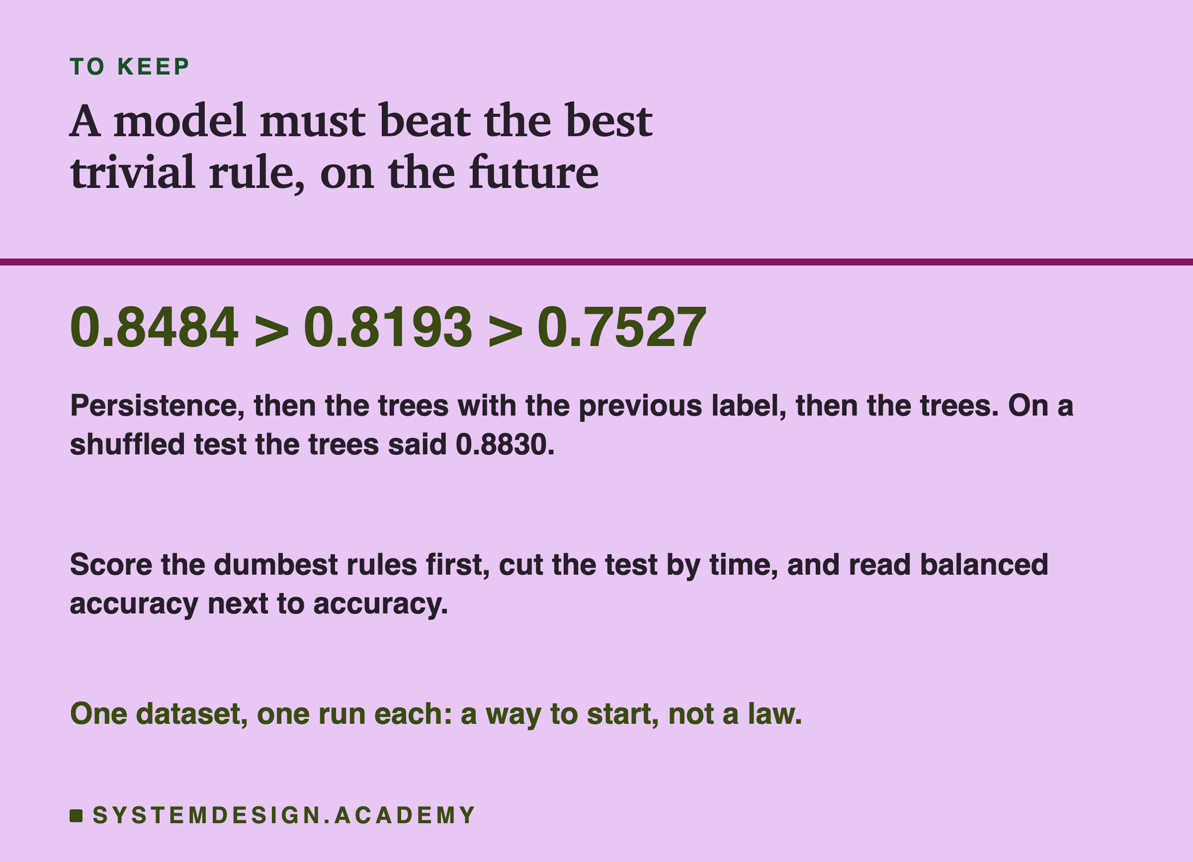
On the future, persistence scored 0.8484. It was the best of all six. The trees plus lag came second at 0.8193, 0.0291 below it. The plain trees scored 0.7527, 0.0957 below. Same period yesterday scored 0.6741, logistic regression 0.6491, and majority 0.5488.

Read that ranking slowly. A rule with no learning beat boosted trees with eight inputs by almost ten points of accuracy. Giving the trees the previous label, the very thing persistence uses, closed most of the gap, but not all of it: the trees with the lag still got 0.0291 less right than the lag on its own.

If I had only trained the trees and reported 0.7527, it would have looked like a reasonable first model: three right out of four, well above the 0.5488 of always saying DOWN. Only the persistence baseline shows that it is worse than doing nothing clever at all. And if I had tested on a shuffle, as later slides show, the trees would have scored 0.8830 and looked better than persistence. Two ordinary shortcuts, skipping the strong baseline and shuffling the test, would each have hidden the result.

The seasonal rule is weaker than persistence here. The label 48 rows back agreed with the current one 65.6% of the time over the whole data, far below the 85.3% of the row just before. Electricity demand has a daily rhythm. My reasoning, not a measurement: this label compares the price with its own last 24 hours, and that average already contains a whole day, so part of the daily rhythm may cancel out.

Accuracy counts every row the same. When one label is more common, that can make a useless rule look fair. The forward test is 54.9% DOWN, so a rule that always says DOWN scores 0.5488 without ever finding an UP row.

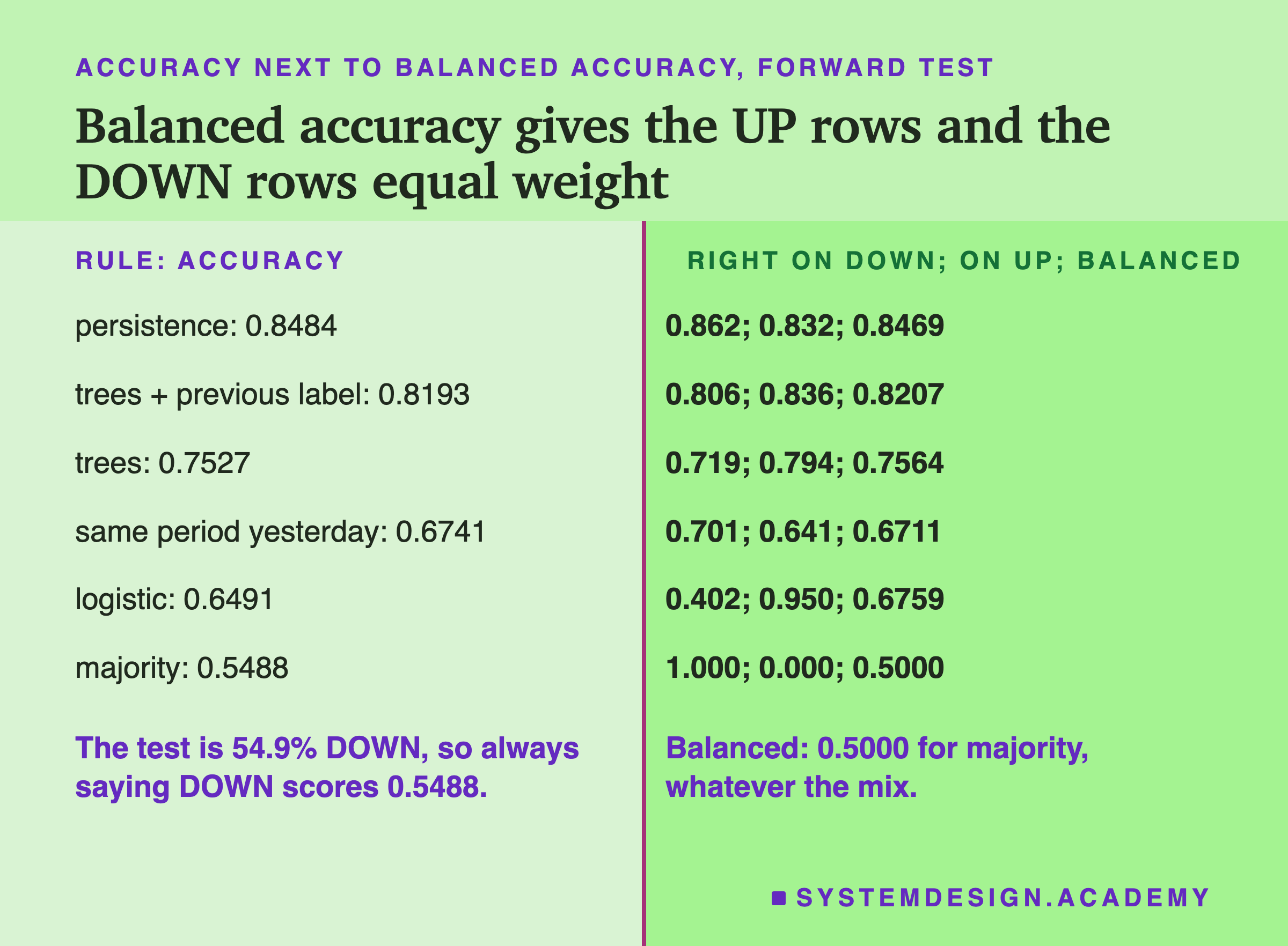
Balanced accuracy fixes that by scoring each label on its own. Take the share of DOWN rows the rule got right, and the share of UP rows it got right (each share is called the recall of that label), and average the two. A rule that always says one label gets 1 on that label and 0 on the other, so its balanced accuracy is always exactly 0.5, however lopsided the test is. That makes 0.5 a fixed floor that anyone can read.

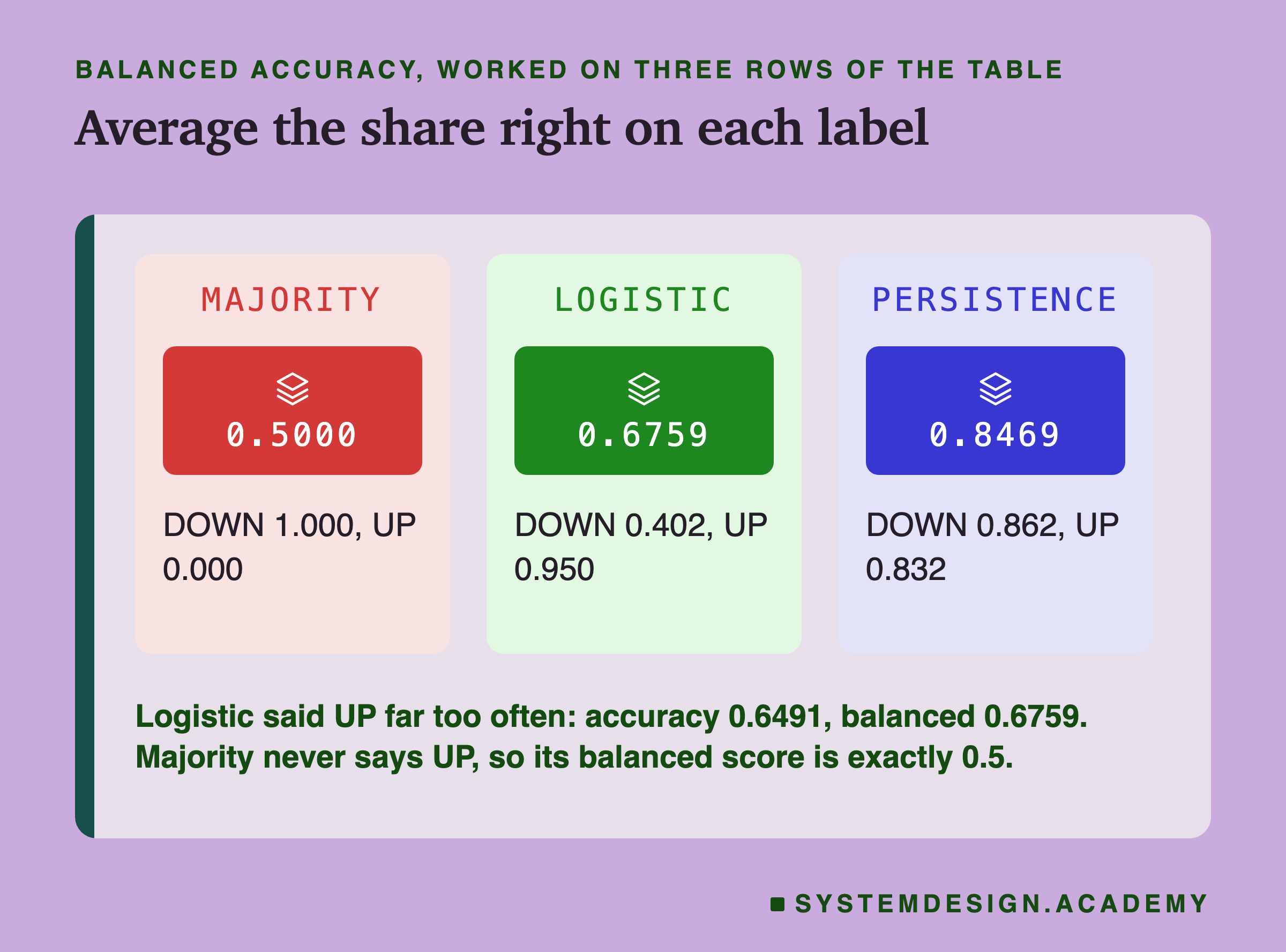
Logistic regression shows what the second number adds. Its accuracy was 0.6491 and its balanced accuracy 0.6759. It was right on 95.0% of UP rows but only 40.2% of DOWN rows: it said UP far too often. Its accuracy hid that lean, and the two recalls show it at once. Persistence, by contrast, was nearly even: 86.2% of DOWN rows and 83.2% of UP rows, balanced 0.8469, close to its accuracy of 0.8484.

On this test, balanced accuracy does not change the order of the six: persistence is still first and majority still last. It changes how far each one sits from doing nothing. Report both: accuracy tells a reader how often the model is right, and balanced accuracy tells them whether it is right about both labels.

Persistence wins when labels repeat. So I measured how strongly they do, over all 45,312 rows. I added these tables after the results.

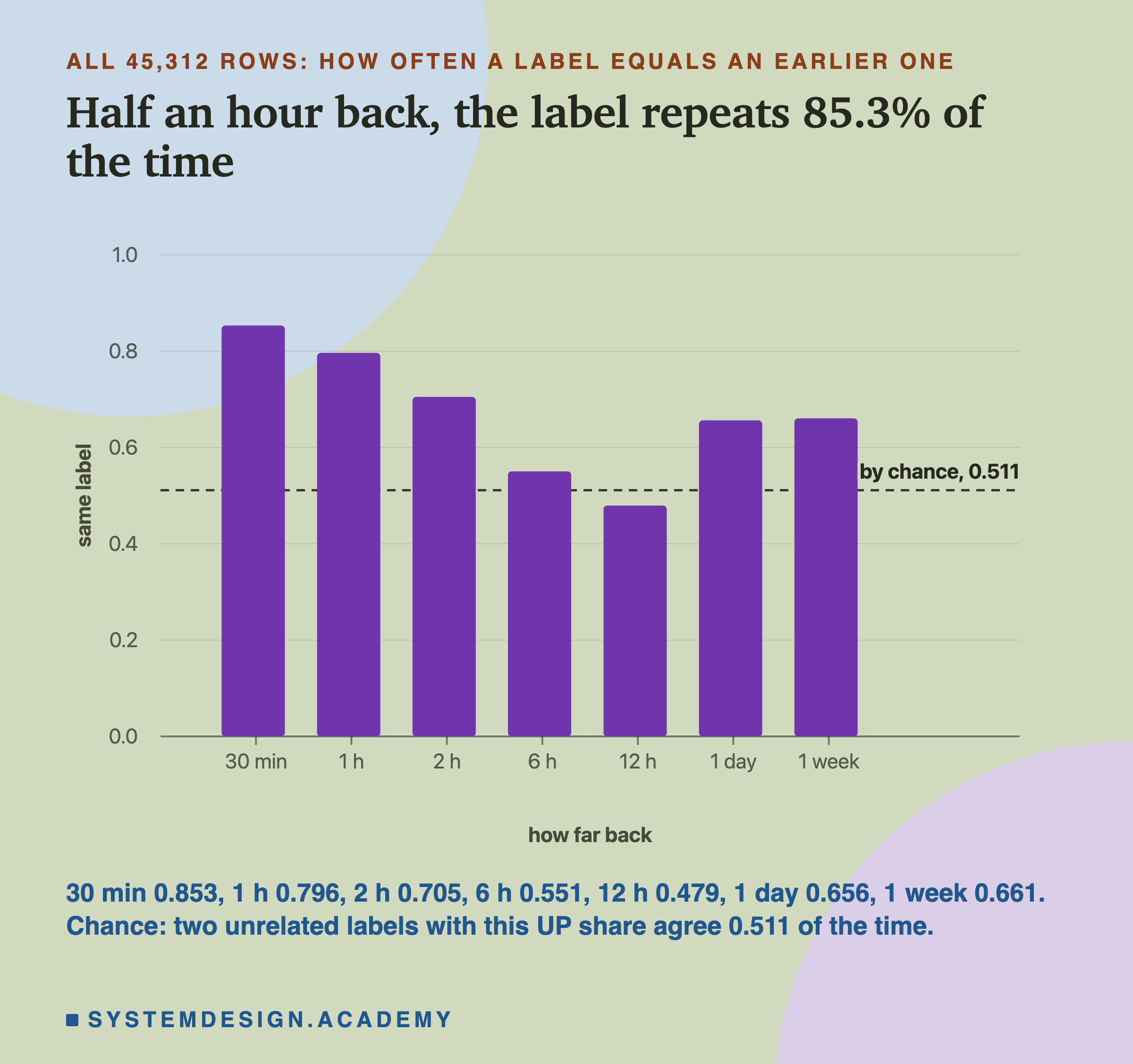
Half an hour back, the label is the same 85.3% of the time. An hour back, 79.6%; two hours, 70.5%; six hours, 55.1%. Twelve hours back it is 47.9%, slightly below chance. Chance here means how often two unrelated labels would agree, given that 42.5% of labels are UP: 0.511. One day back it rises again to 65.6%, and one week back to 66.1%. So the label has a strong short memory, fading over a few hours, and a weaker daily one.

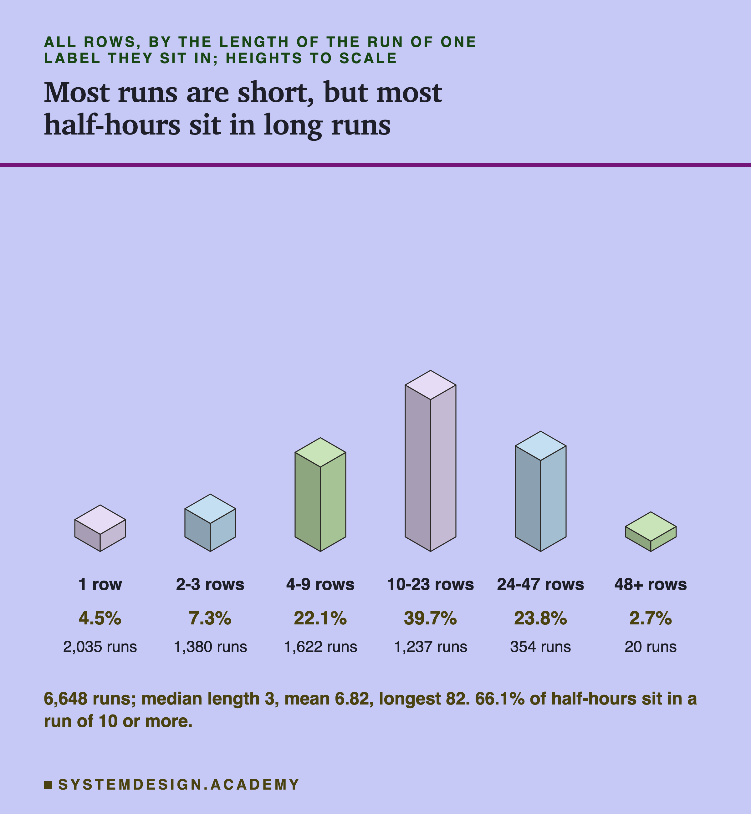
A run is a stretch of rows with the same label, one after another. The data holds 6,648 runs. Most are short: the median run is 3 rows long, and 2,035 runs are a single row. But most half-hours sit in long runs: 66.1% of all rows are inside a run of 10 or more, which is five hours or longer. The longest run was 82 rows. DOWN runs were longer on average than UP runs, 7.84 rows against 5.79.

Those two facts together explain persistence's score. Inside a long run it is right on every row but the first. It loses one row per run, and with 6,648 runs in 45,312 rows, that is about one row in seven.

Persistence has one weakness, and it is exact. It is wrong on a row if and only if the label flipped on that row. In the forward test, 1,374 of the 9,063 rows were flips, 15.2%. Persistence was wrong on all 1,374 and right on all 7,689 others. Its accuracy, 0.8484, is simply one minus the share of flips; the report checks that.

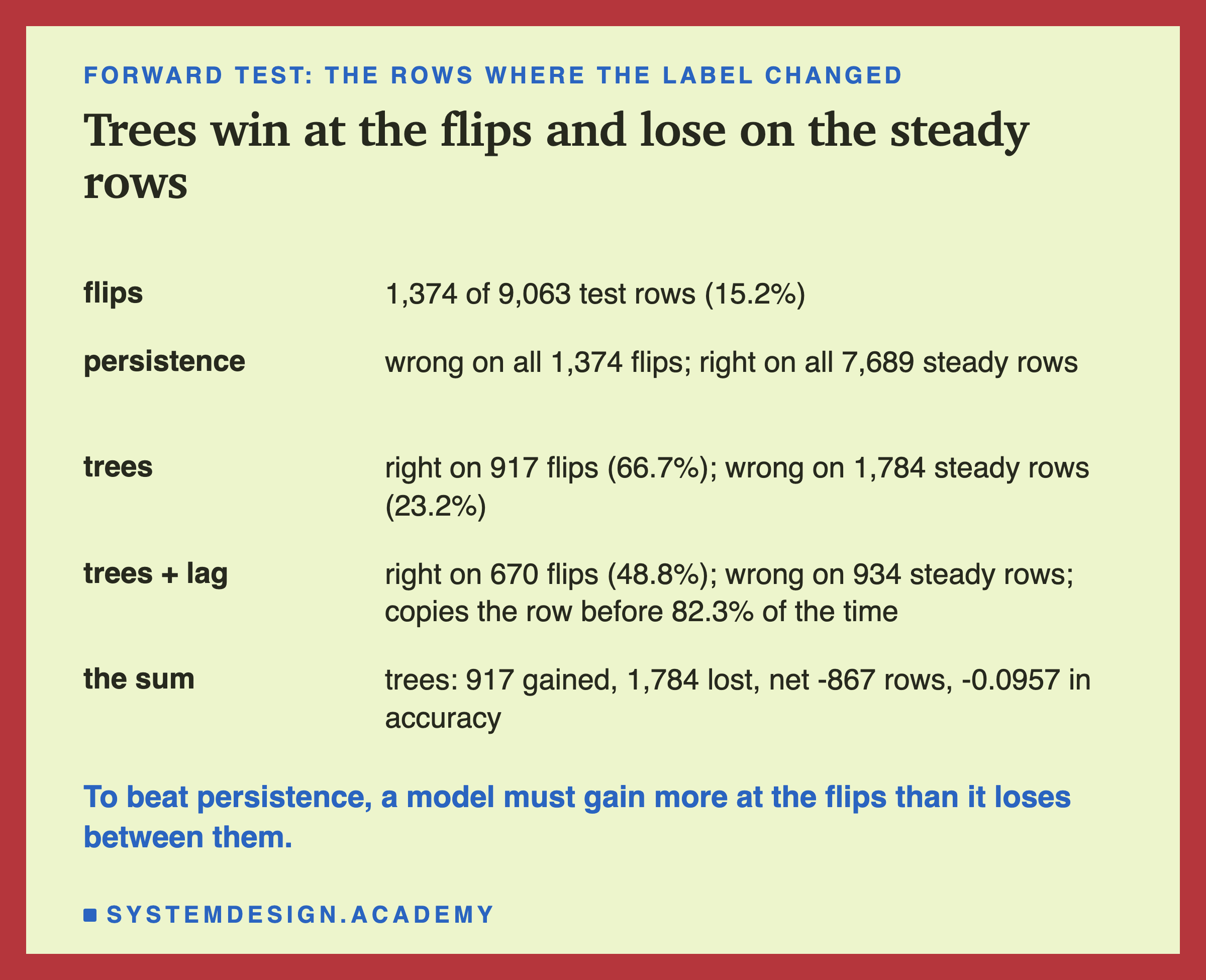
So a model can only beat persistence at the flips. On every other row persistence is already right, so the best a model can do there is match it. The question is whether a model gains more at the flips than it gives away on the steady rows.

The trees did something persistence cannot: they were right on 917 of the 1,374 flips, 66.7%. But they were wrong on 1,784 of the 7,689 steady rows, where persistence was right. They gained 917 rows and lost 1,784, a net loss of 867 rows, which is exactly the 0.0957 gap in accuracy. The trees plus lag behaved more like persistence: they repeated the previous label on 82.3% of rows, got 670 flips right (48.8%) and gave away 934 steady rows, a smaller net loss.

This is the most useful way I know to read a model against persistence: split the test into flips and steady rows and count both columns. It also says where a better model would have to come from. Any real improvement over persistence lives in the 15.2% of rows where something changed.

After the results, I cut the forward test into eight blocks of three hours each and scored persistence, the trees and the trees plus lag on each block. The data does not say whether the first period of a day starts at midnight or ends at 00:30; I count it as 00:00, so the clock times below may be half an hour early.

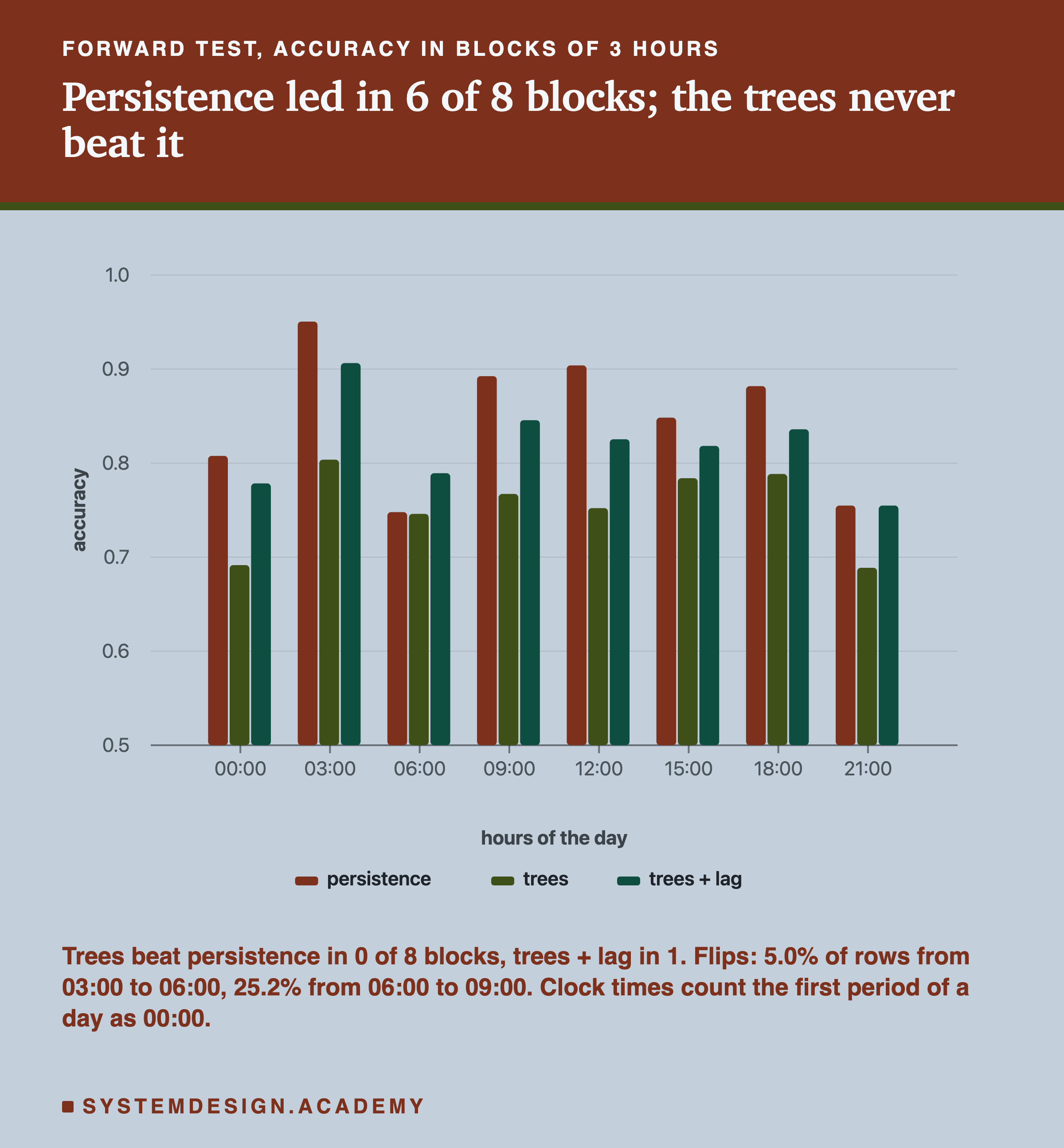
The plain trees did not beat persistence in any block of the day. The trees plus lag beat it in one, from 06:00 to 09:00: 0.789 against 0.748, and tied it from 21:00 to midnight at 0.755. That is also the block with the most flips: 25.2% of its rows changed label, the most of any block. The block from 21:00 to midnight was close behind at 24.5%. From 03:00 to 06:00 only 5.0% of rows flipped, and persistence scored 0.950 there.

That fits the flips slide. Where the label rarely changes, persistence is very hard to beat. Where it changes often, persistence is weakest, and that is the only place a model with more information had a chance. One possible reason the mornings flip so often, and it is a guess I did not test, is that demand rises quickly then, and the price crosses its slow 24-hour average as it climbs.

The same comparison by calendar month, using the rebuilt dates. Also added after the results.

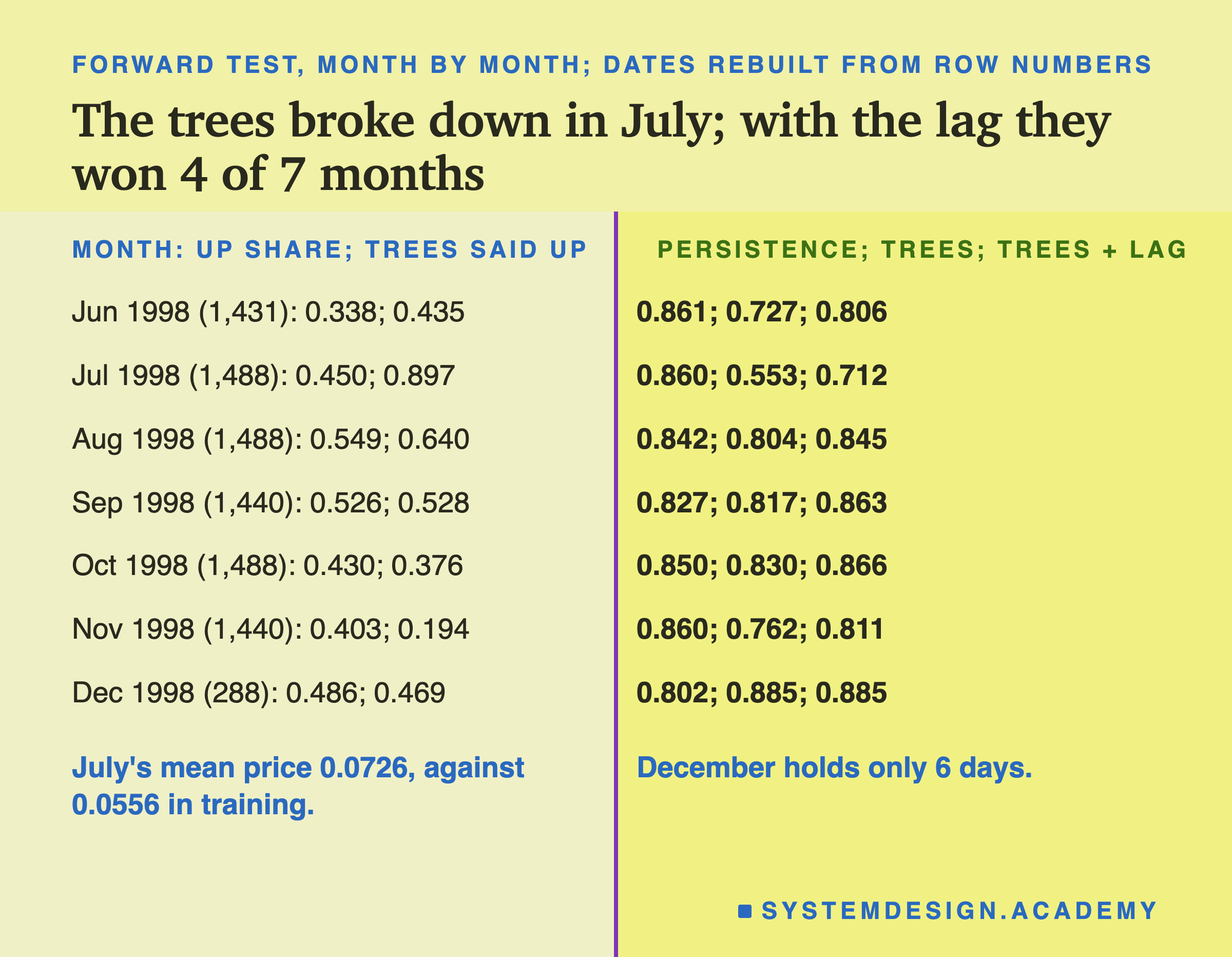
Persistence was steady from month to month: between 0.802 and 0.861. The trees were not. In July 1998 their accuracy fell to 0.553, barely above a coin. In that month only 45.0% of rows were UP, but the trees called 89.7% of them UP. The trees plus lag fell too, to 0.712. The plain trees beat persistence in only one month, December, which holds just 6 days (288 rows). The trees plus lag beat it in 4 of the 7 months: August by 0.003, September by 0.036, October by 0.015, and December.

Why July? What I measured: July's average NSW price was 0.0726 on the scaled range, against 0.0556 over all the training rows, and the trees said UP on nine rows in ten. One possible reason, and it is a guess: the trees learned that a high price usually means UP. But UP means high compared with the last 24 hours, not high in general. In a month when all prices were high, every price looked high to the trees. November fits the same idea only loosely: the trees said UP on just 19.4% of rows against 40.3% that were, although November's average price, 0.0554, was close to training's. August argues against it too: its average price, 0.0753, was higher than July's, yet the trees scored 0.804 there and said UP on 64.0% of rows against 54.9% that were. December's average, 0.0691, was also above training's, and the trees scored 0.885. So the price level is not the whole story, and I have not tested the guess.

What is not a guess: a monthly table showed a failure that the overall accuracy of 0.7527 averaged away, and persistence, which never looks at a price, had no such month. A rule that uses less information can also have fewer ways to break.

The lab also scored each model on a random 80/20 split. The forward scores and the shuffled scores are very different, and the shuffle flatters the models: it makes them look better than they will be in use.

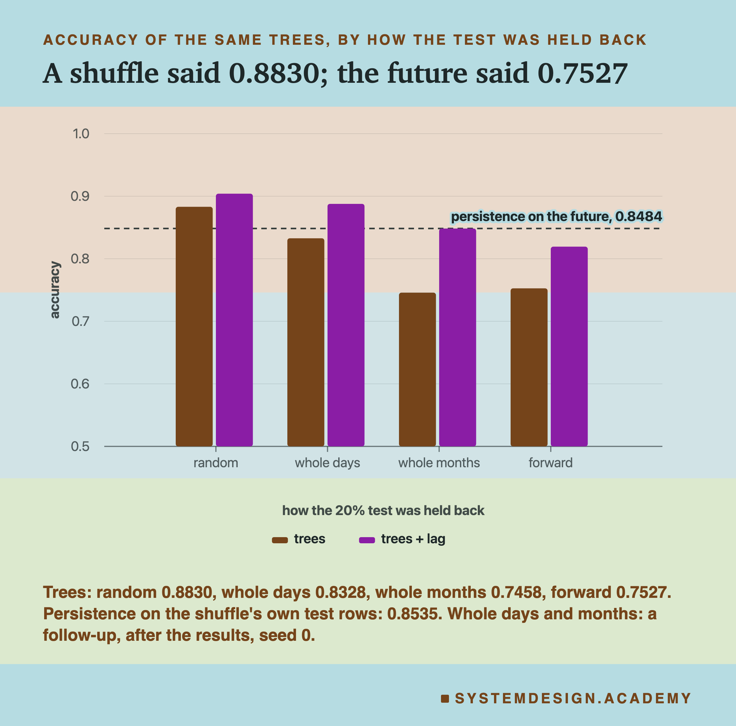
On the shuffle, the trees scored 0.8830; on the future, 0.7527, a gap of 0.1303. The trees plus lag went from 0.9040 to 0.8193, and logistic regression from 0.7579 to 0.6491. Look at what that does to the ranking. Scored on the shuffle's own test rows, persistence gets 0.8535, so like for like the shuffled trees (0.8830) and trees plus lag (0.9040) are both ahead of it. A team that tested on a shuffle would have concluded that the trees beat persistence, and shipped a model that loses to it on the future.

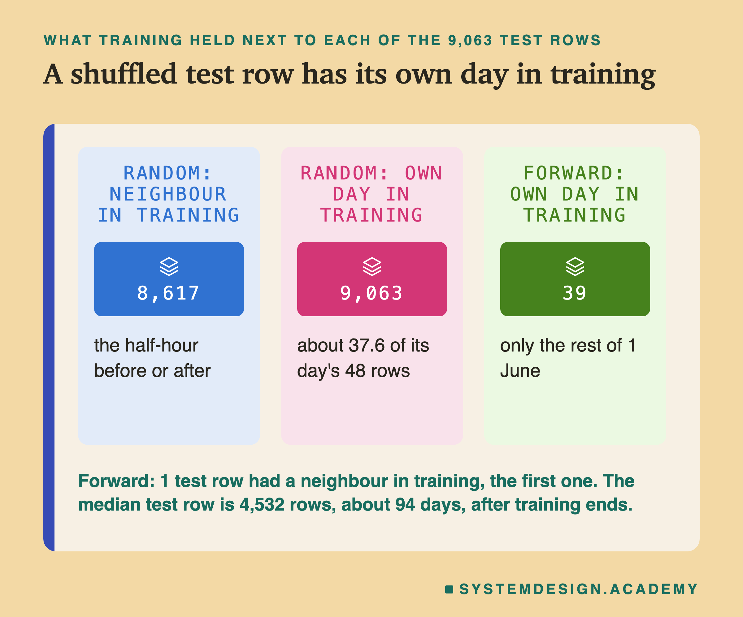
The score that lied measured why this happens on bike rentals, and the same thing is at work here. With a random split, 8,617 of the 9,063 test rows had the half-hour just before or just after them in training, and every one of the 9,063 had other rows of its own day in training: on average about 37.6 of that day's 48 half-hours. With the forward split, one test row had a neighbour in training (the first one), and 39 test rows shared a day with training, the rest of 1 June. The median forward test row came 4,532 rows, about 94 days, after the last training row.

Counts show what training held, not what the model used, so I ran a follow-up. I designed it after the main results, wrote its design into the report's file before it ran, and ran it once with seed 0. It uses random splits again, but keeps whole groups on one side, so that no test row has any row of its group in training. Keeping whole days together dropped the trees from 0.8830 to 0.8328. Keeping whole calendar months together dropped them to 0.7458, about the same as the forward 0.7527. Here, unlike the bikes, holding out whole months removed nearly all of the shuffle's advantage (0.7458 against the forward 0.7527), and whole days alone removed about 40% of it (0.050 of the 0.130 gap). With the bikes, whole months closed only about half the gap. The whole-month split still trains on months that come after its test months, which the future never allows. In the whole-days split the trees plus lag (0.8878) beat persistence on the same test rows (0.8587); in the whole-months split they were level (0.8483 against 0.8468). One seed, so read these as sizes, not exact amounts.

A review of this lesson asked two questions that the lab's design had not covered, so I added a follow-up to the lab. It was designed after the main results, prompted by that review; its design is the description of the lab's followup mode, and its results are in results/baseline_followup.json.

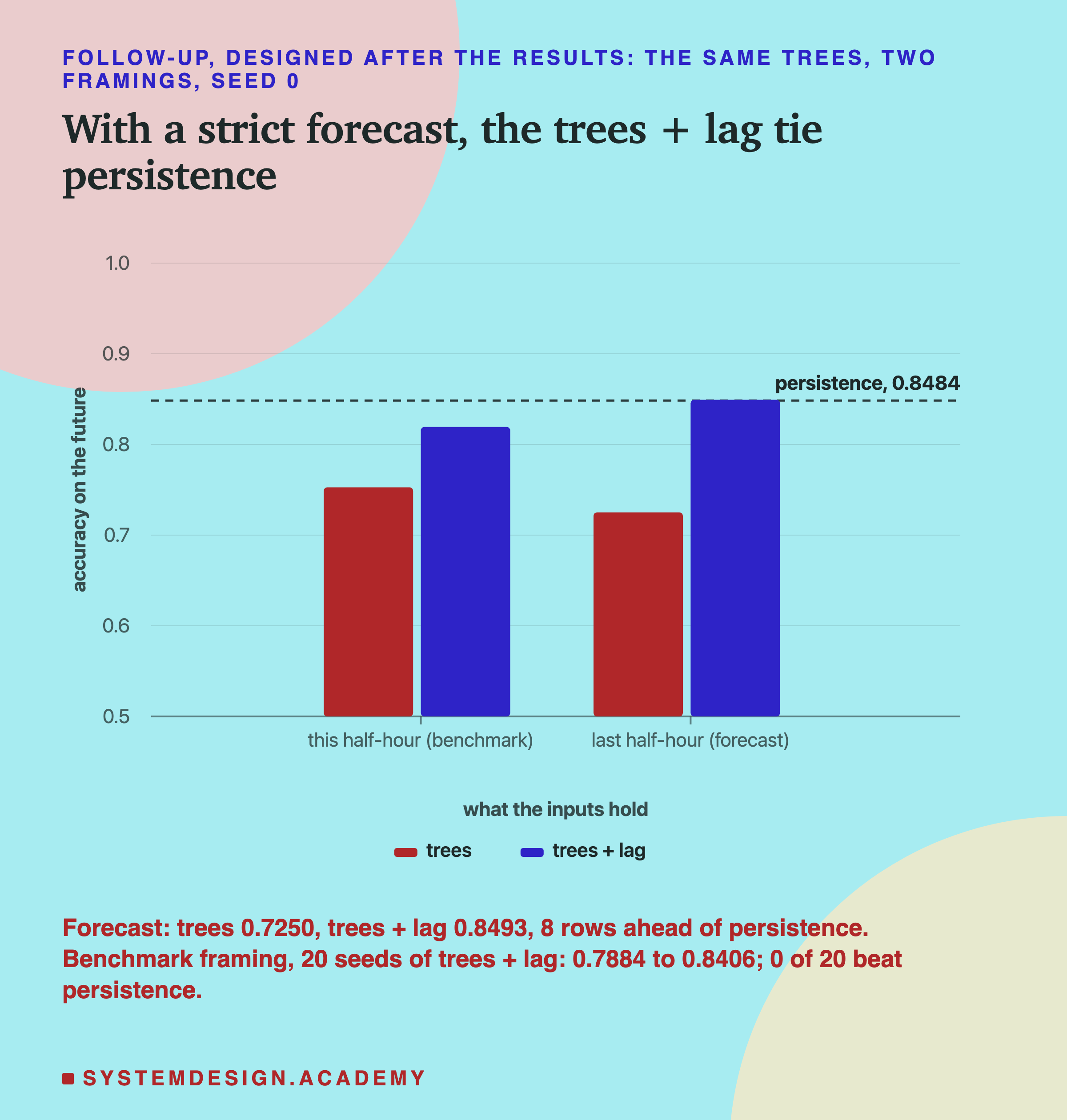
A strict forecast. The benchmark gives the models the prices and demands of the same half-hour whose label they must guess. A strict forecast would only know the previous half-hour's market. So the follow-up moved all five market inputs (the NSW price and demand, the Victoria price and demand, and the transfer) back by one row, and trained the trees again with seed 0. The plain trees fell from 0.7527 to 0.7250. The trees plus lag scored 0.8493 against persistence's 0.8484: 8 rows ahead out of 9,063, which I read as a tie. So the current price did not clearly help the trees, and whether the trees plus lag lose to persistence or tie with it depends on the framing. One run each; I do not know why the two framings moved in different directions, and I will not guess from one run.

Twenty seeds. Every model in the main lab ran once, with seed 0. The trees use their seed to choose which training rows to hold back when deciding how many trees to build, so another seed gives a slightly different model. The follow-up trained the trees plus lag with seeds 0 to 19, in the benchmark's framing. They scored from 0.7884 to 0.8406, with a mean of 0.8091, and none of the 20 beat persistence; the best was still 0.0078 below it. Seed 0, the one in the headline, scored 0.8193, above the mean. How much a score moves from seed to seed is a subject of its own, and the next lesson planned for this chapter measures it.

What this changes. The headline, that persistence beat every model, holds for all 20 seeds in the benchmark's framing. In a strict forecast it becomes a tie for the best model. Either way, no model in this lesson clearly beat the rule that learns nothing.

The rule of this lesson is short: a model must beat the best trivial rule on a forward test before anything else. Here is what that asks, in the order a team meets it.

Say what is known when each guess is made. Persistence was fair here only because the previous half-hour's label is known before the next guess. Write that down, because it decides which rules count as trivial. In this lab it also showed that the models were given the current half-hour's price, from which the label is computed; with the market one half-hour old, the best model tied persistence instead of losing to it.

Score several rules, and keep the best. Majority is the one everyone scores and the weakest here, at 0.5488. Persistence was the strongest at 0.8484, and the seasonal rule was in between at 0.6741. If I had scored only majority, the trees at 0.7527 would have looked like a fine model.

Use the forward test for all of them. A rule and a model scored on different tests cannot be compared. The shuffle raised the trees by 0.1303; persistence, which has no training at all, moved only from 0.8484 to 0.8535, because the shuffled test holds different rows.

When no model wins, say so. Here the answer to "is the model good enough?" was no. The honest next steps are to ship the rule, to add what the rule knows to the model (the lag closed most of the gap), or to reframe the problem, for example to predict only the flips, where persistence is always wrong. What I would not do is report the shuffled 0.8830.

This script is the lab made small. It downloads the same data, scores majority and persistence on the forward test, trains the boosted trees on the first 80% and scores them on the last 20%. It does not need a GPU.

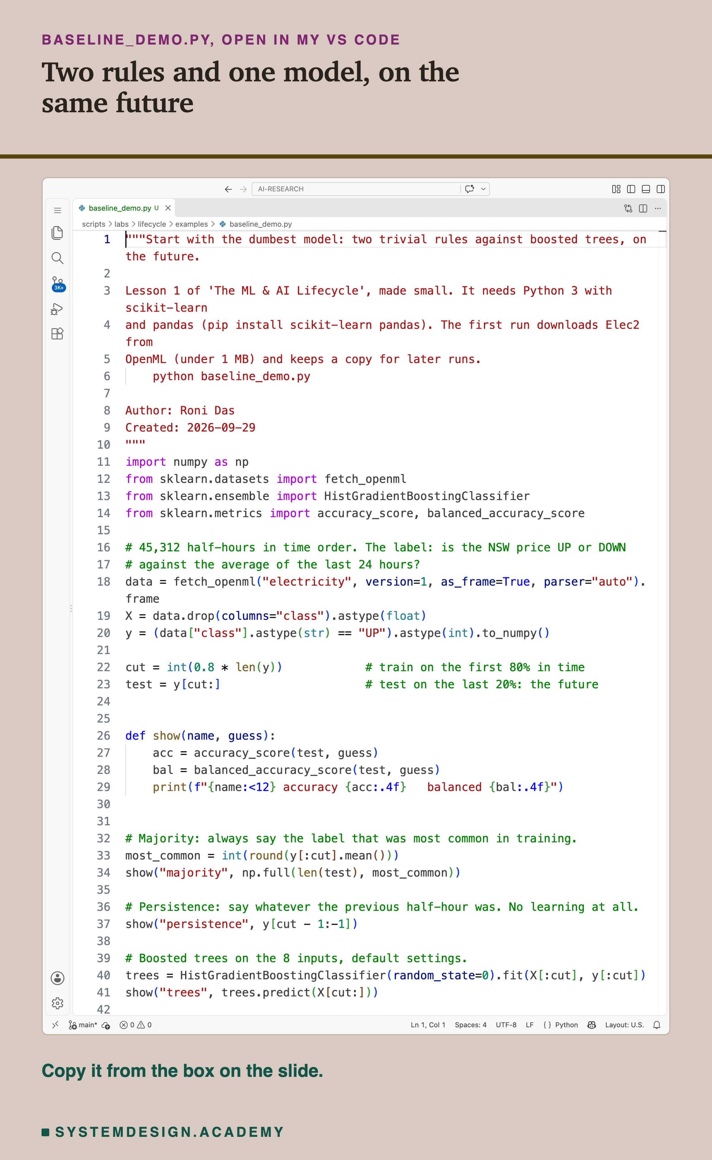
Before you run this lab. You need Python 3 and two libraries: pip install scikit-learn pandas. scikit-learn holds the model, the scores and the download; pandas holds the table. The first run downloads Elec2 from OpenML (under 1 MB compressed), so it needs an internet connection once; scikit-learn keeps a copy in a folder in your home directory (scikit_learn_data) for later runs. I ran it with scikit-learn 1.9.1 on a Mac. scikit-learn runs the same way on Windows and Linux, but I have not checked the numbers there, and another version of scikit-learn may give slightly different decimals for the trees. The two rules need no library beyond NumPy, which scikit-learn installs.

"""Start with the dumbest model: two trivial rules against boosted trees, on the future.

Lesson 1 of 'The ML & AI Lifecycle', made small. It needs Python 3 with scikit-learn
and pandas (pip install scikit-learn pandas). The first run downloads Elec2 from
OpenML (under 1 MB) and keeps a copy for later runs.
    python baseline_demo.py

Author: Roni Das
Created: 2026-09-29
"""
import numpy as np
from sklearn.datasets import fetch_openml
from sklearn.ensemble import HistGradientBoostingClassifier
from sklearn.metrics import accuracy_score, balanced_accuracy_score

# 45,312 half-hours in time order. The label: is the NSW price UP or DOWN
# against the average of the last 24 hours?
data = fetch_openml("electricity", version=1, as_frame=True, parser="auto").frame
X = data.drop(columns="class").astype(float)
y = (data["class"].astype(str) == "UP").astype(int).to_numpy()

cut = int(0.8 * len(y))            # train on the first 80% in time
test = y[cut:]                     # test on the last 20%: the future


def show(name, guess):
    acc = accuracy_score(test, guess)
    bal = balanced_accuracy_score(test, guess)
    print(f"{name:<12} accuracy {acc:.4f}   balanced {bal:.4f}")


# Majority: always say the label that was most common in training.
most_common = int(round(y[:cut].mean()))
show("majority", np.full(len(test), most_common))

# Persistence: say whatever the previous half-hour was. No learning at all.
show("persistence", y[cut - 1:-1])

# Boosted trees on the 8 inputs, default settings.
trees = HistGradientBoostingClassifier(random_state=0).fit(X[:cut], y[:cut])
show("trees", trees.predict(X[cut:]))

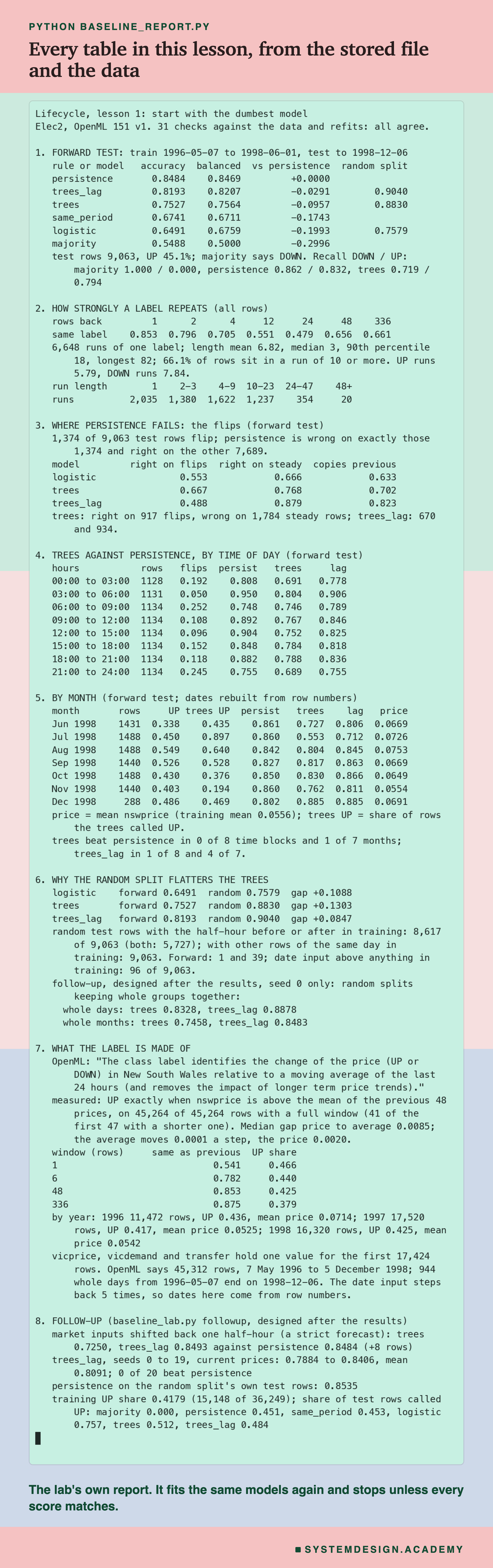
The report lives in scripts/labs/lifecycle/baseline_report.py. It reads the lab's stored file, results/baseline.json, and the Elec2 data from scikit-learn's local copy. The lab stored scores, not each guess, so to read the guesses by flip, by time of day and by month, the report fits the same three models again with the same data, settings and seeds. It stops unless every forward and random accuracy it gets is the stored one to twelve decimal places. It makes 31 such checks in all, including the check that the label is the 24-hour rule, and they all agree. It changes nothing in baseline.json.

Its json mode writes every number to results/bl-report.json, which the figures read. The blocked mode is the follow-up on the random-split slide; its design is in the report's own docstring and its results are in results/baseline_blocked.json. The demo mode checks the student script's stored run, and the mode writes the playground below and checks that it gives the lab's scores.

This box has no model in it. It holds the 9,063 forward test labels, one character each (1 for UP, 0 for DOWN), and the boosted trees' stored guess for each one, recomputed by the report and checked against the lab's score. It runs in your browser.

As it is, the box prints the accuracy and balanced accuracy of majority, persistence and the trees, which the report's box mode checks against baseline.json, and then the flips: 1,374 in 9,063 rows, with the trees right on 917 of them.

Try by_hours() to see persistence and the trees in blocks of three hours, and by_hours(6) for blocks of six. Then write your own rule: any list of 9,063 guesses of 0 or 1 can go into score. For example, score([1] * len(LABELS)) scores always saying UP; its balanced accuracy is exactly 0.5, like majority's. A fair rule may only use the labels before each row, which is what rule does with past[i], the label of the row before row i.

Loading. fetch_openml("electricity", version=1) downloads Elec2 once and reads it from the local copy after that. The label column holds the words UP and DOWN, so the script turns it into 1 and 0. The eight inputs become plain numbers with astype(float), which is also what the lab did.

The cut. cut = int(0.8 * len(y)) is 36,249. The test is every row from there to the end, in order. Nothing is shuffled anywhere in the script.

Majority. round(y[:cut].mean()) is the share of UP in training, 0.4179 (15,148 of 36,249 rows), rounded to 0, so the rule says DOWN for every test row. It only looks at training rows, as a fair baseline must.

Persistence. y[cut - 1:-1] takes the labels from the last training row up to the second-to-last row. Laid next to the test labels y[cut:], each test row is paired with the label of the row before it. It is one slice and no learning.

The trees. HistGradientBoostingClassifier(random_state=0) with default settings, trained on the first 36,249 rows and asked about the rest. The fixed seed matters: the trees hold back part of the training rows to decide when to stop adding trees, and the seed fixes which rows.

The scores. show prints accuracy and balanced accuracy with four decimals, in lines well under 80 characters, so they fit an ordinary terminal.

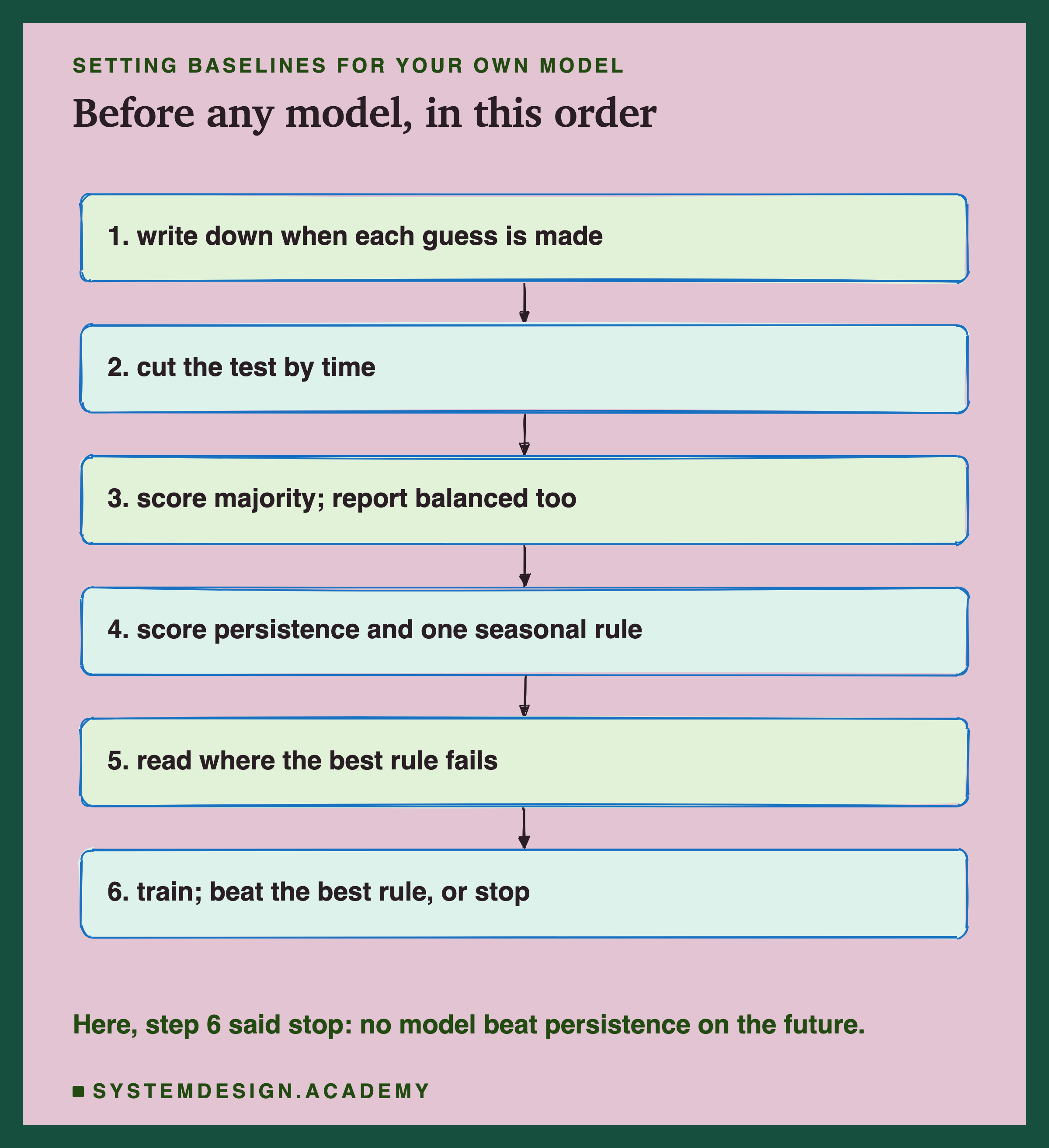
Write down when each guess is made. List what is known at that moment: which labels have arrived, which inputs exist yet. That list decides which rules are fair and which inputs a model may use.

Cut the test by time. If rows arrive in time order and the model will meet later rows, train on the earlier part and test on the later part, for every rule and every model.

Score majority, and report balanced accuracy next to accuracy. Majority gives the floor, and balanced accuracy puts that floor at 0.5 whatever the mix of labels.

Score persistence and at least one seasonal rule. Pick the season from the data's own rhythm: a day for half-hourly data, a week for daily sales. Measure how often a label equals the one before it; if that share is high, persistence will be hard to beat.

Read where the best rule fails. For persistence, that is the flips. Count them. They are the only rows where a model can gain.

Train, then compare against the best rule, not the weakest. Split the model's result into rows where it beat the rule and rows where it lost. If it does not come out ahead on the future, stop and decide: ship the rule, give the model what the rule knows, or frame the problem again.

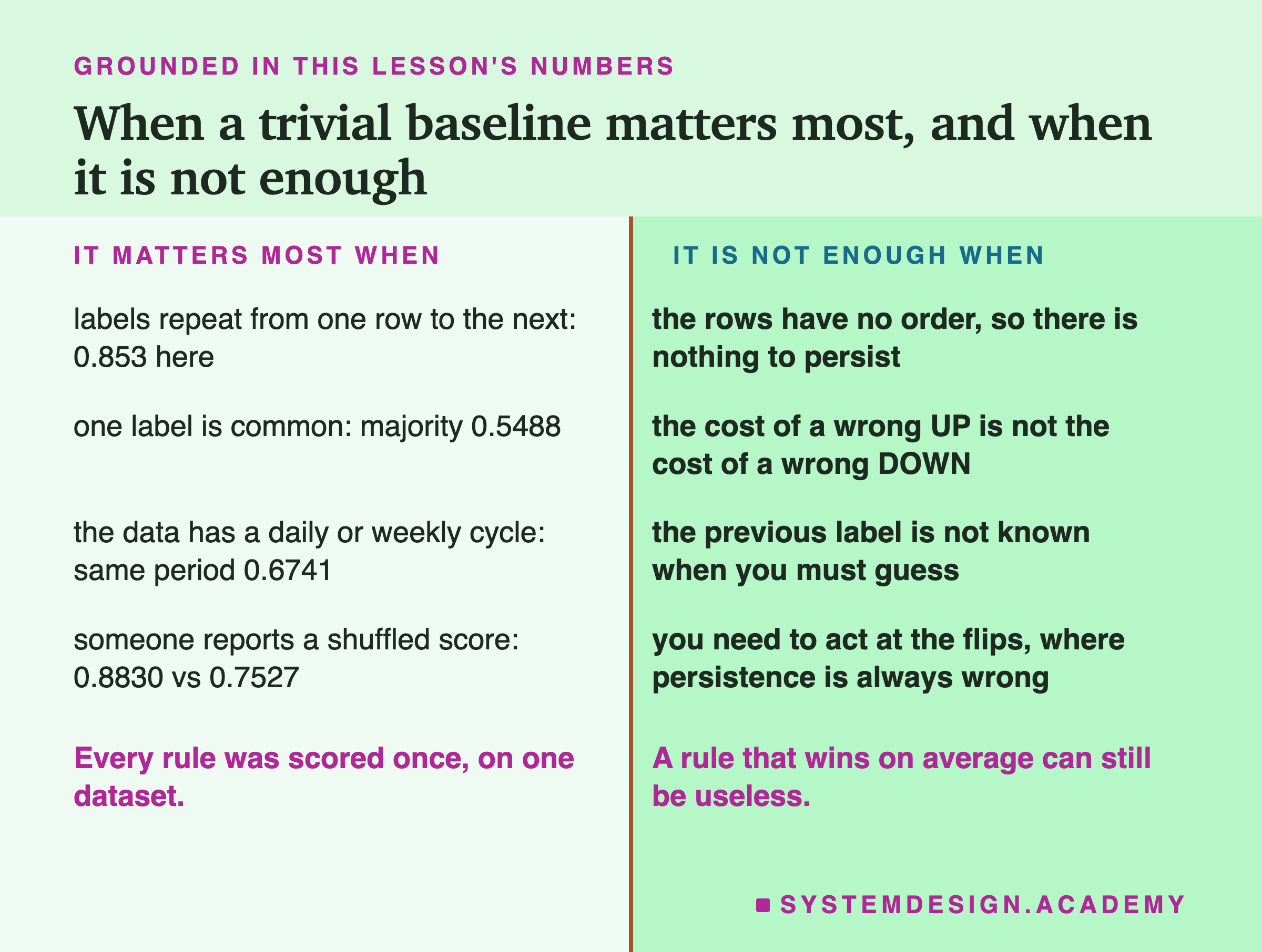
Use strong baselines when rows come in time order and labels repeat. Prices, sensor states, demand above or below normal, whether a server is busy. Here the label equalled the previous one 85.3% of the time, and persistence beat every model.

Use them when one label is common. Fraud, faults, rare events. Majority will score high on accuracy, so report balanced accuracy, where it scores exactly 0.5.

Use a seasonal rule when the data has a cycle. Daily and weekly rhythms are common in anything people do. Here it was weaker than persistence (0.6741), but that is something to measure, not assume.

Use them whenever someone shows you a single score. Ask what persistence and majority got on the same test, and whether the test was cut by time. Here that one question turns 0.8830 into a loss.

Do not stop at a baseline when the rows have no order. If each row is an independent case, such as one loan application, there is nothing to persist, and majority is the main trivial rule.

Do not stop there when errors cost different amounts, or when the flips are the job. A rule that is right 85% of the time can be useless if the rows it misses are the only ones that matter, as with an alarm that must fire when a price turns. Persistence never predicts a change. If your use needs changes, score the model on the flips, where persistence scores zero.

Do not use persistence when the previous label is not known in time. If labels arrive late, persist the last label you would really have, and score that.

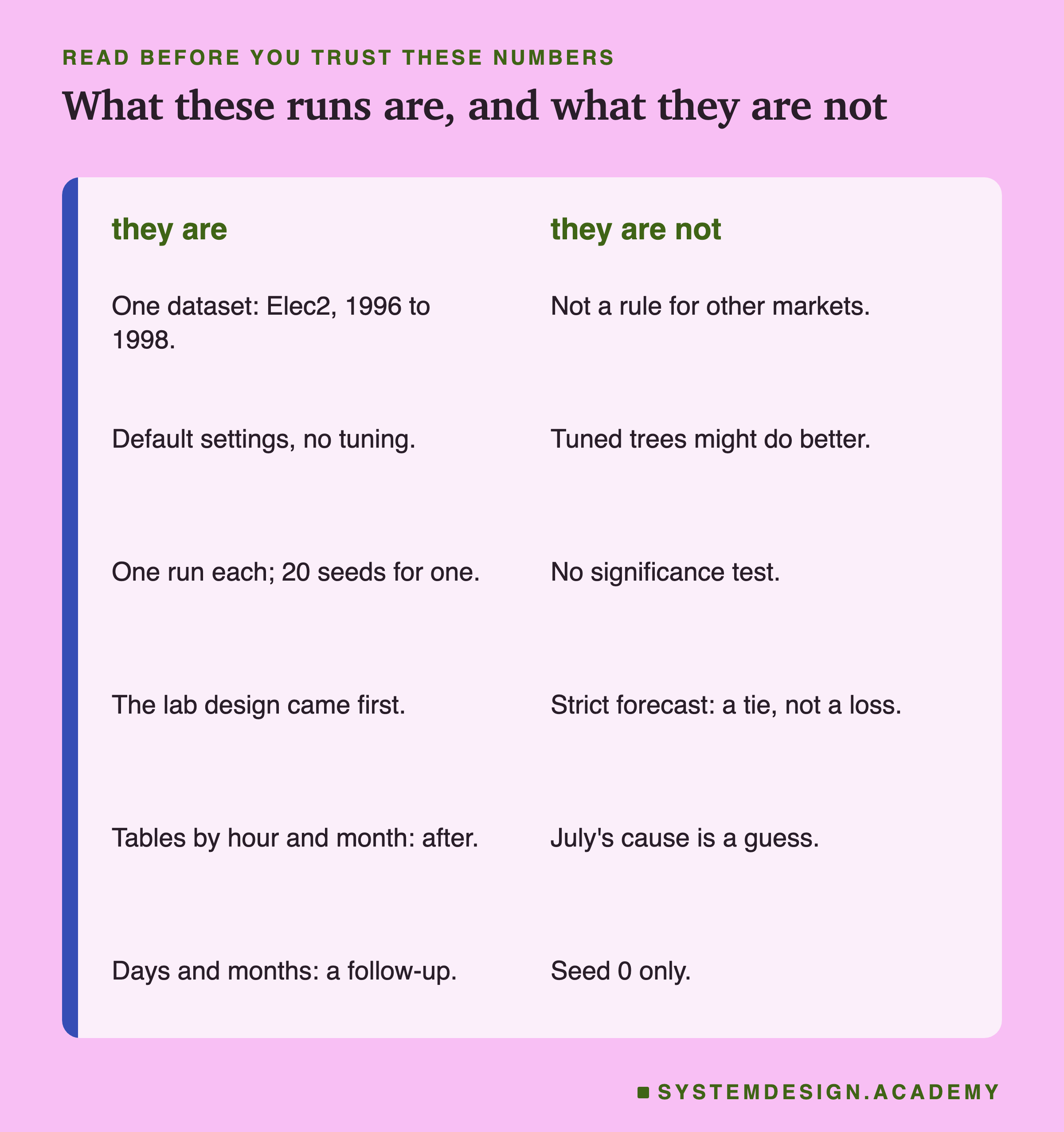
One dataset, one market, two and a half years. Elec2 is a well-known public dataset from one electricity market in the 1990s. On data where labels repeat less, persistence would be weaker, and a model might win easily. The result here is about this data.

Default settings, one run each, no significance test. No model was tuned. A tuned model, or one given more lags (the labels two, three or 48 rows back), might beat persistence; I did not test that. Each score is one run, except the follow-up's 20 seeds of the trees plus lag, and I declared no significance test before running, so I do not call any gap significant.

The label is sticky by its own definition, and the models saw the current price. Both are properties of how the benchmark was built, measured here: the label is exactly the price against the average of the previous 48 prices, and the models' inputs include the current price. The headline, persistence ahead of every model, is a result about that framing. In the follow-up's strict forecast, with every market input one half-hour old, the trees plus lag tied persistence instead (0.8493 against 0.8484) and the plain trees fell to 0.7250. One run each, so I do not read a direction into either change.

Designs before, tables after. The lab's design was written before it ran. Everything past the six headline scores was added after I saw them: the lag and run tables, the flips, the tables by time of day and by month, and the labels built from other windows. The whole-day and whole-month splits are a follow-up designed after the results, with one seed.

Guesses stay guesses. Why the trees broke in July, and why mornings flip often, are my guesses. I have not tested either.

The dates are rebuilt. The file has no clean calendar, so the months and hours come from row numbers, checked against the weekday column. If a day were missing from the file, the months would shift; the weekday check makes that unlikely but cannot rule out a whole missing week.

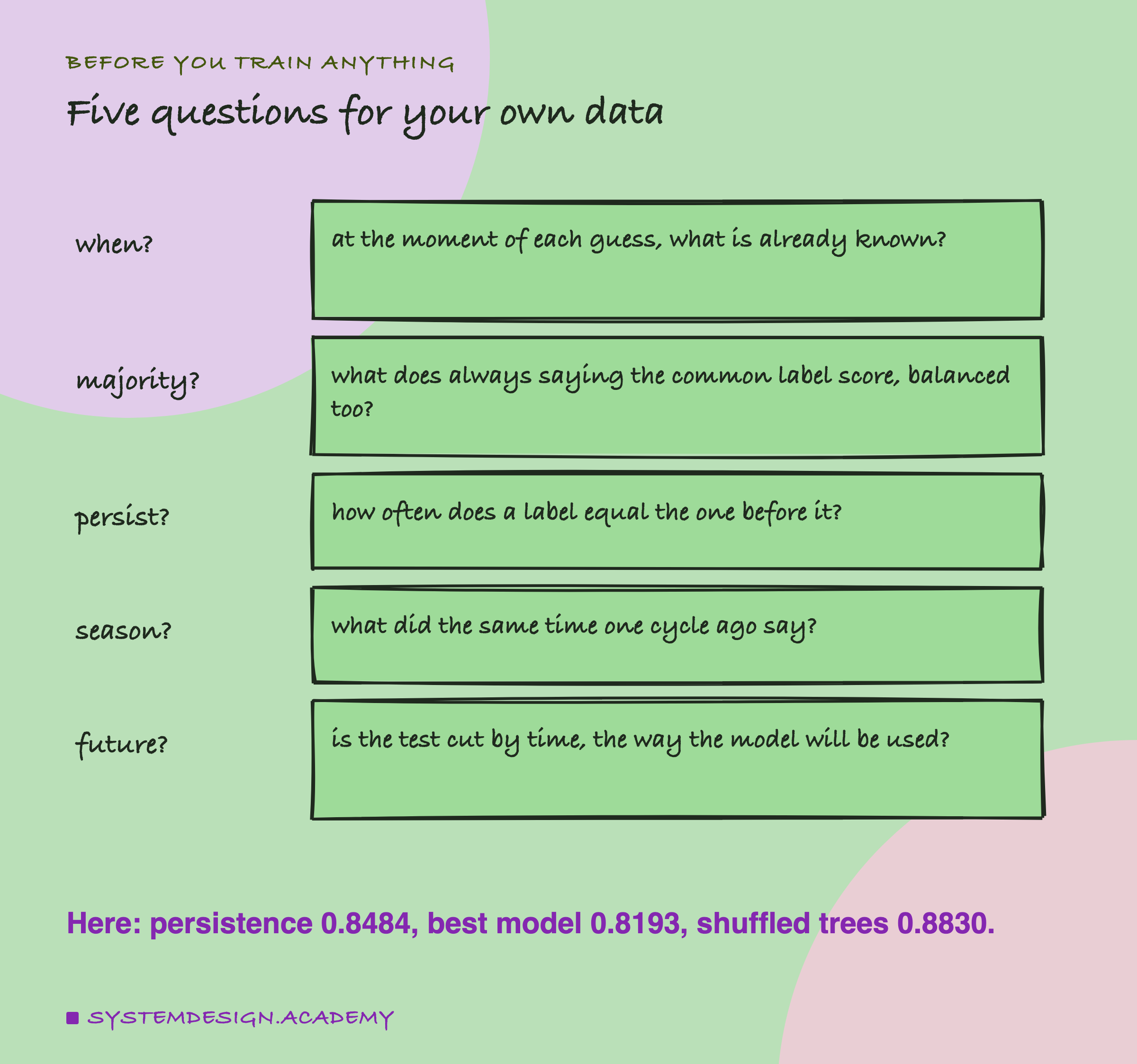
Take one model that you or your team has trained, and find its test score. Then ask the five questions on the card. The second and third take a few lines each, and they run in seconds.

If persistence or majority comes close to your model, that is not a failure to hide. It is the most useful thing you can learn before shipping: it tells you where your model can add something (for persistence, only at the flips) and gives you a simple fallback to ship instead.

The next lesson planned for this chapter stays at the training step and asks a question this lesson did not: if I train the same model twice, on the same data, with the same code, do I get the same model? Here every model ran once with a fixed seed. The next lesson measures what changes when that seed does, and what else changes between two runs that look identical.