Imagine you stay with a friend and she tells you how she likes her toast: "put the dial on 5". On her toaster the dial goes from 1 to 10, so 5 is the middle: golden brown. You go home, put bread in your own toaster and set its dial to 5. Your toaster's dial only goes from 1 to 6. On it, 5 is nearly the hottest setting.

A few minutes later the toast is black, smoke is coming out of the toaster, and the smoke alarm on the ceiling goes off. Someone is waving a towel at it while the person at the stove wonders what happened.

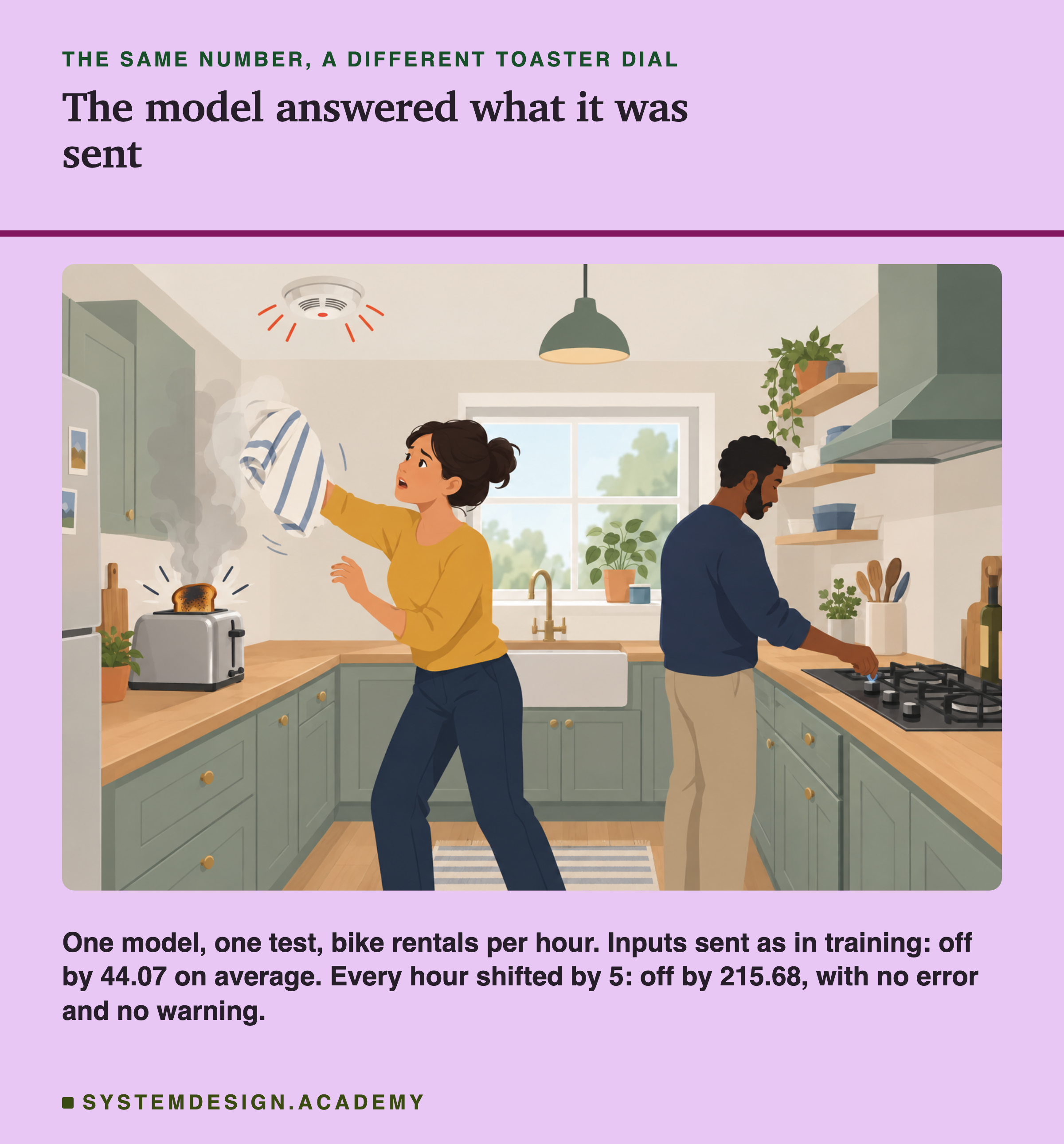
Notice what did not go wrong. Your friend's advice was right for her toaster. Your toaster worked perfectly. Nobody made a mistake in their own kitchen. The only problem was the number passed between them: 5 meant one thing where it was said and another thing where it was used. And the toaster did not complain. A toaster heats to the setting it is given.

A program that learned from examples behaves like that toaster. It was trained on numbers computed one way. When it is used, the numbers may be computed in a slightly different way, by different code. It does not refuse and it does not warn. It answers. In this lesson I measure how wrong those answers get, for six ordinary ways that the same number can be computed twice.

This is the third lesson of the chapter, and it uses the same public data as the first two: two years of hourly bike rentals from Washington, D.C. The first lesson showed that a fair test must keep time in order, and with that fair test the program missed by 44.07 bikes an hour on average. The second lesson showed that the world itself moves: more people rented bikes in the second year, and a program that never learned again fell behind.

This lesson looks at a different kind of failure. Nothing about the world changes here. The test hours are the same hours as in lesson 1, the real answers are the same, and the program is the same program, trained once, with the same settings. The only thing that changes is the code that prepares the program's inputs at the moment it is used.

That code is often written later than the training code, by another person or another team, sometimes in another programming language, sometimes by a data provider you never meet. It is supposed to produce exactly the numbers the training code produced. When it does not, the program is being asked about a slightly different world from the one it learned, and nothing tells you so. The words for all of this come next.

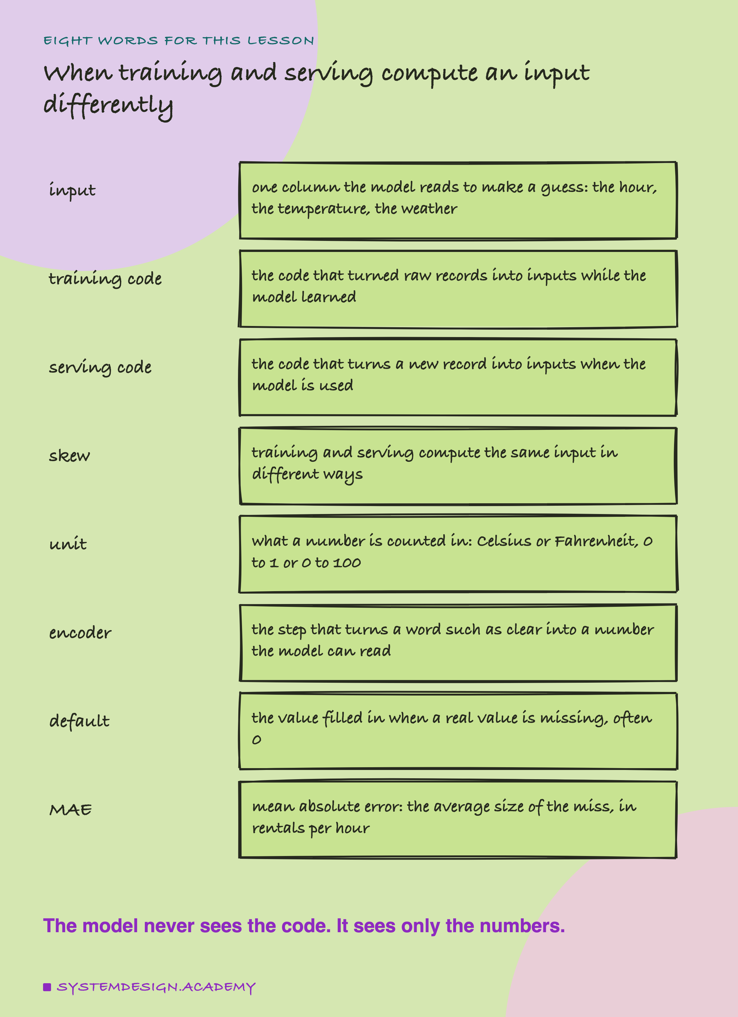
A model is a program that learned from examples to guess a number, here the bikes rented in one hour. Each thing it reads to make a guess is an input, sometimes called a feature: the hour of the day, the temperature, the humidity, a weather word such as clear or misty. This model reads 12 inputs.

Before the model can learn, some code has to turn raw records (a timestamp, a sensor reading, a weather report) into those 12 inputs. I call that the training code. When the model is used, which is called serving it, other code does the same job for each new record: the serving code. Train/serve skew is the name for what happens when those two pieces of code compute the same input in different ways. The model is the same; the numbers it is fed are not.

A unit is what a number is counted in: degrees Celsius or Fahrenheit, a fraction from 0 to 1 or a percentage from 0 to 100. A time zone decides which hour a moment is called: 8 in the morning in Washington is 12 or 13 o'clock in UTC, the world's reference time. An encoder is the step that turns a word such as clear into a number, because the model only reads numbers. A default is the value filled in when the real value is missing, very often 0. The baseline is the score to compare against: here the model with correct inputs. Last, as in the earlier lessons, the MAE (mean absolute error) is the average size of the miss in rentals per hour, and the signed error keeps the sign, so it shows whether the guesses lean too high or too low.

Here is the idea in one picture, using the first hour of the lab's test: 12 noon on a day in August 2012.

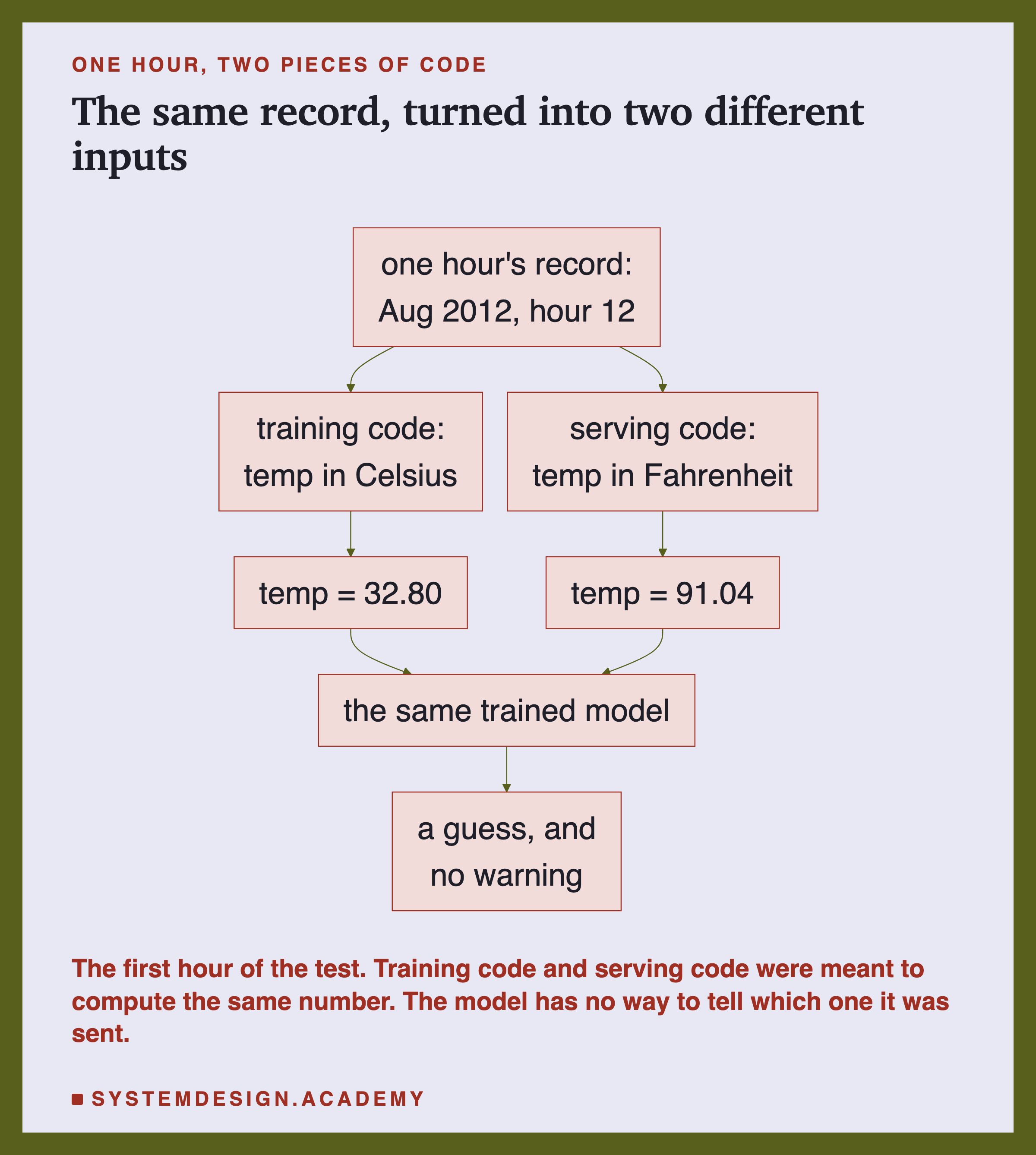
The raw record says it was hot that hour. The training code wrote the temperature as 32.8, in Celsius, the way the dataset stores it. Imagine the serving code gets its weather from a different provider that reports Fahrenheit, and nobody converts it. Then it sends 91.04 for the same hour. Both numbers are correct descriptions of the same afternoon. To the model they are two different afternoons, and one of them is hotter than anything it ever saw.

The causes are ordinary. Real teams run into all of these:

• Units. One system stores Celsius, another Fahrenheit. One stores humidity as 0.55, another as 55. One stores money in dollars, another in cents.
• Time zones. The training data was stored in local time; the live service runs on a server clock set to UTC. The same moment gets a different hour.
• Numbering. Is Sunday day 0 or day 6? Is January month 0 or month 1? Different libraries answer differently.
• Spelling of labels. Training saw "clear"; the live feed sends "Clear" or "CLEAR" or "sunny".
• Missing values. Training dropped rows with no wind reading; serving fills the gap with 0 because that was the default in some other code.

None of these is exotic. Each is one line of code written by a careful person who did not know what the other code did.

I wrote the design at the top of the lab file, skew_lab.py, before I ran it, and the chapter plan, CHAPTER-PLAN.md, records it the same day ("SKEW LAB (batch 3) designed before running"). Here is what it says.

The model and the test. The same boosted trees as lesson 1: scikit-learn's HistGradientBoostingRegressor, default settings, random_state=0. A decision tree guesses a number by asking a chain of yes-or-no questions about the inputs; boosting adds up many small trees, each correcting the ones before. The model is trained once, on the first 80% of the hours in time order (13,903 hours, January 2011 to August 2012). Every condition is scored on the same last 20%: 3,476 hours from August 2012 to the end of December 2012. This is lesson 1's forward test: the model is tested only on hours that came after all of its training hours, the way it would be used.

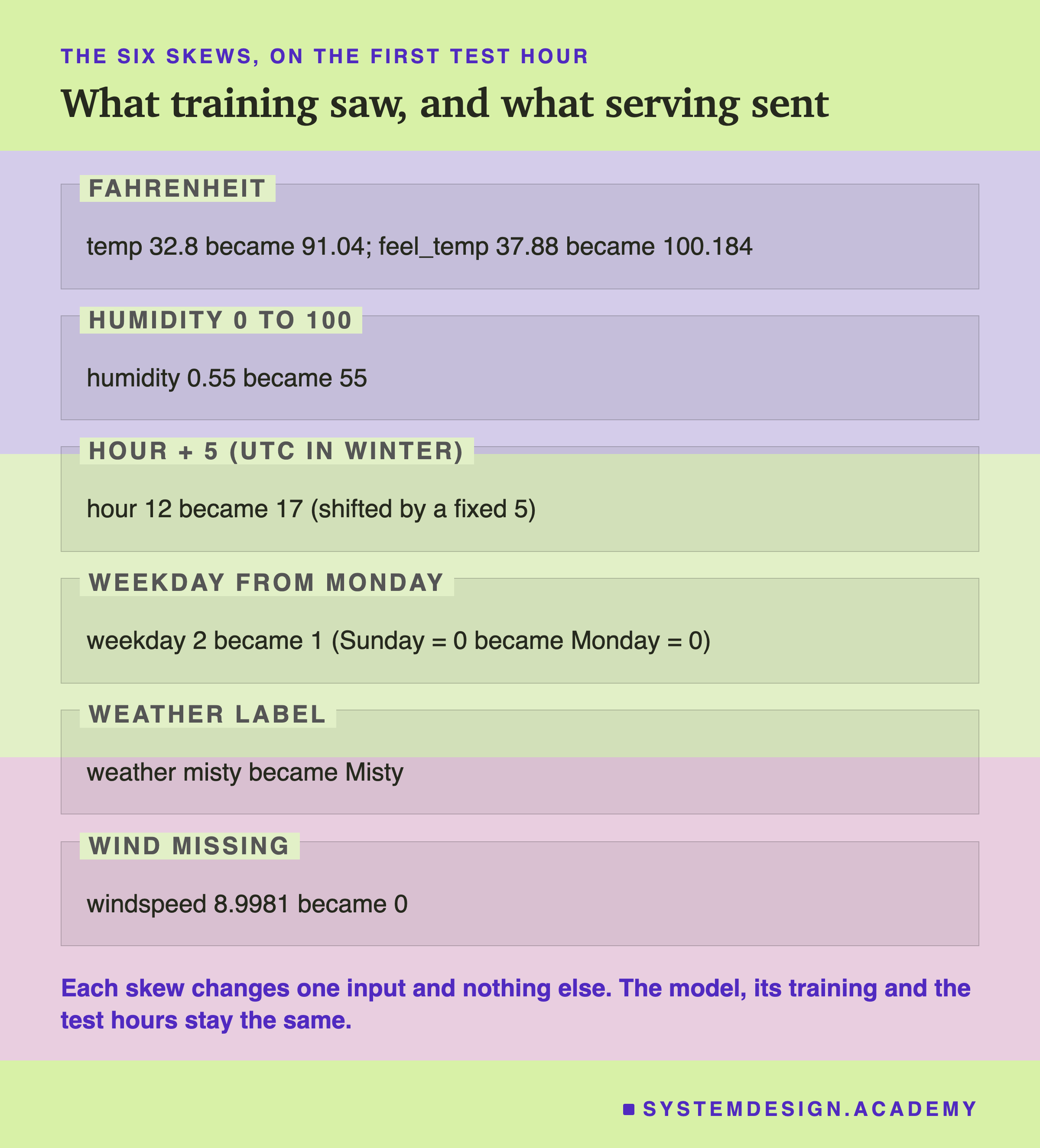
The seven conditions. "none" sends the inputs exactly as in training, so its score must be lesson 1's forward score, and it is: 44.07. The report checks that its 3,476 stored guesses are the very guesses lesson 1 stored. Then six skews, each applied to the serving inputs only: temperatures in Fahrenheit (both temp and feel_temp); humidity as a percentage; every hour shifted by a fixed +5, wrapping past midnight, which is what converting to UTC does in winter (Washington is 5 hours behind UTC in winter but only 4 in summer, so for the summer and autumn hours of the test the +5 is not real UTC; a follow-up below measures the real offset); the weekday counted from Monday = 0 instead of the dataset's Sunday = 0; the weather label with a capital first letter; and a missing wind speed filled with 0.

What it records. For each condition: the MAE, the signed error, the share of hours whose guess moved by more than 10 bikes from the "none" guess, the lowest and highest guess, and how many guesses were below zero. It also stores every single guess, which is what the rest of the lesson reads.

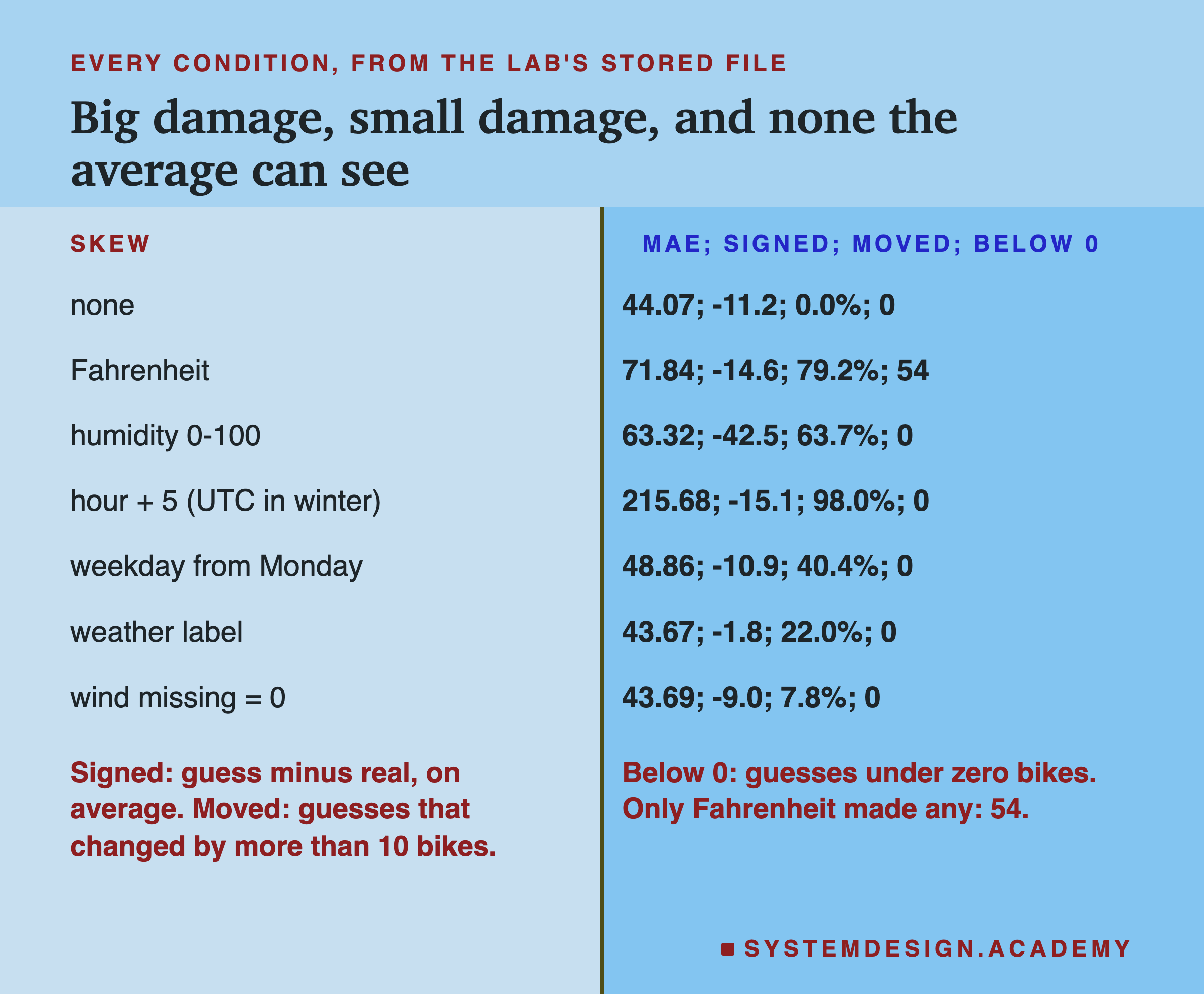
Here is the headline, from the lab's stored file, results/skew.json.

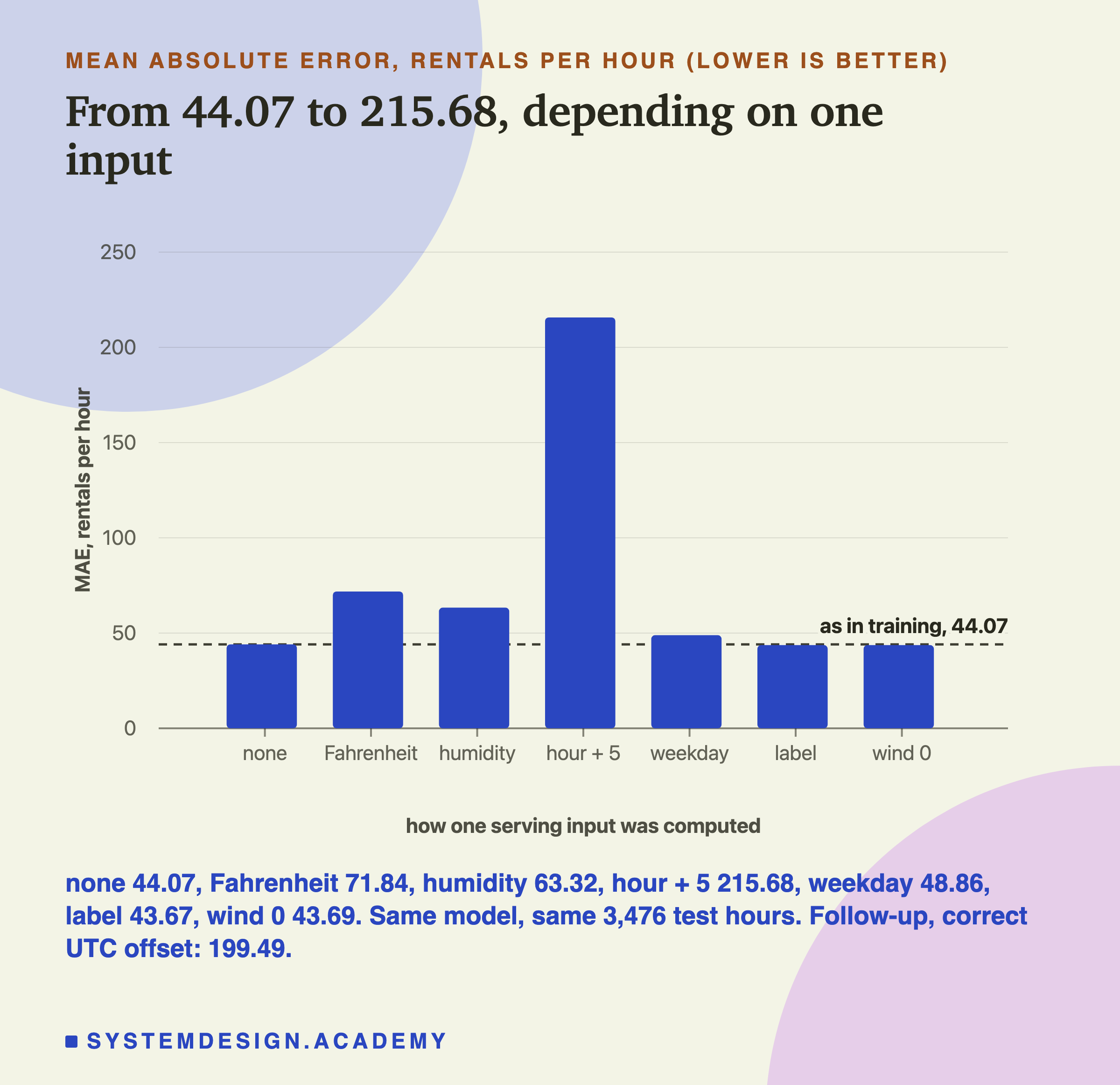
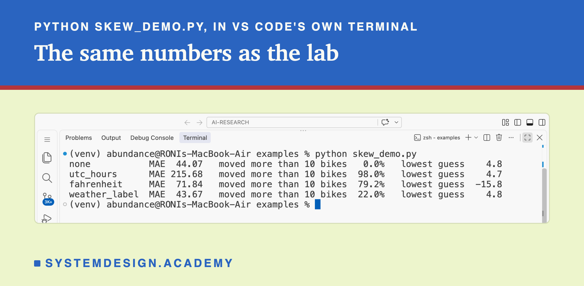
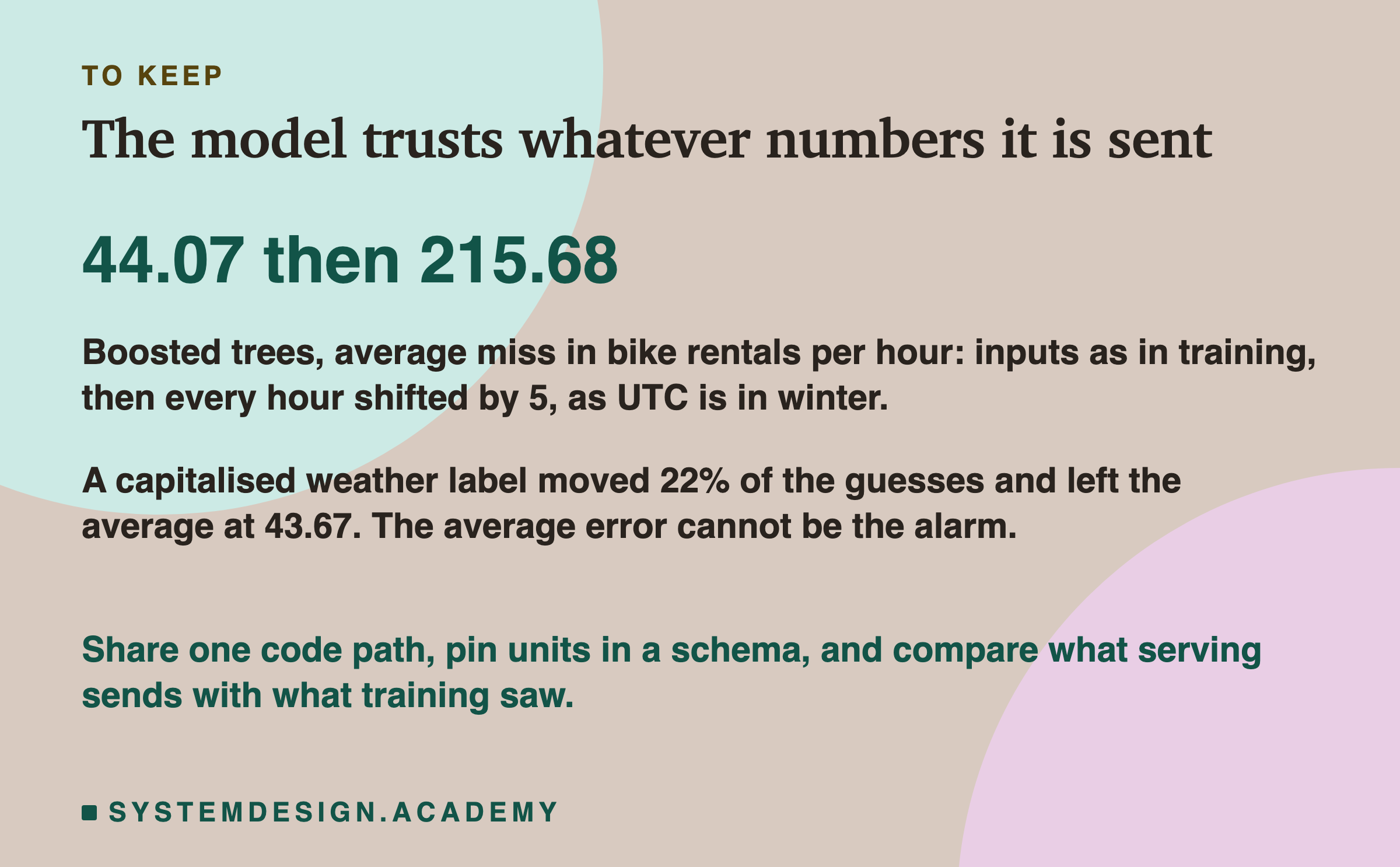
With the inputs as in training, the model missed by 44.07 rentals an hour on average. Shifting every hour by 5 made it 215.68, 4.89 times as much. Temperatures in Fahrenheit gave 71.84, humidity as a percentage 63.32, and the weekday counted from Monday 48.86. Two skews left the average where it was: the capitalised weather label gave 43.67 and the missing wind speed 43.69, both very slightly under the baseline.

Same model, same hours, same real answers. One input computed differently, and the damage runs from none that the average can see to almost five times the error.

A review of this lesson pointed out that a fixed +5 is not real UTC for most of the test: Washington was 4 hours behind UTC until 4 November 2012, and 60.1% of the test hours fall before that date. So I added a follow-up to the lab, designed after the main results and prompted by that review (skew_lab.py followup, results in results/skew_followup.json). With the correct offset, +4 before 4 November and +5 after, the MAE was 199.49, 4.53 times the baseline, with a signed error of -14.0. Real UTC does almost as much damage as the fixed shift. The rest of the lesson reads the main run's fixed +5, which I call "hours shifted by 5".

The worst skew is the natural place to look for an obvious sign of trouble. There is none.

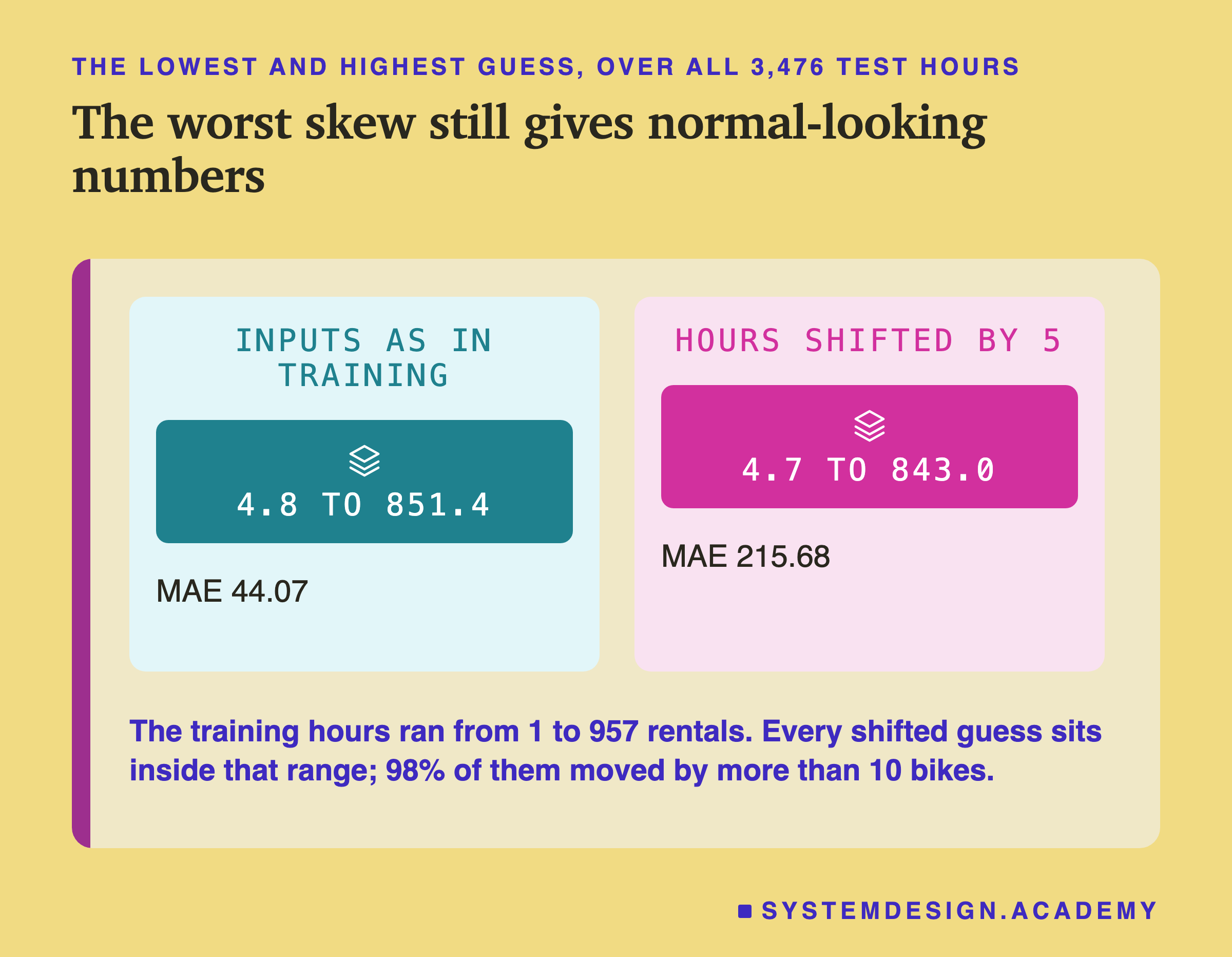
With the inputs as in training, the guesses over the 3,476 test hours ran from 4.8 to 851.4 rentals. With every hour shifted by 5, they ran from 4.7 to 843.0. The training hours had real counts from 1 to 957. Every shifted guess is a number that could be true. Nothing is negative, nothing is huge, nothing is empty. If you looked at a dashboard of these guesses, it would look like a normal day of bike rentals. It is a normal day. It is just the wrong hours of it.

This is the part of skew that surprises people. A model has no idea what its inputs mean. It has only learned which ranges of numbers went with which answers. Given a number, it looks up the answer it learned for that range and returns it, with the same confidence as always. The boosted trees in this lab never raise an error for an input they have not seen; a tree simply sends every value down one side or the other of each question. Many other models behave the same way.

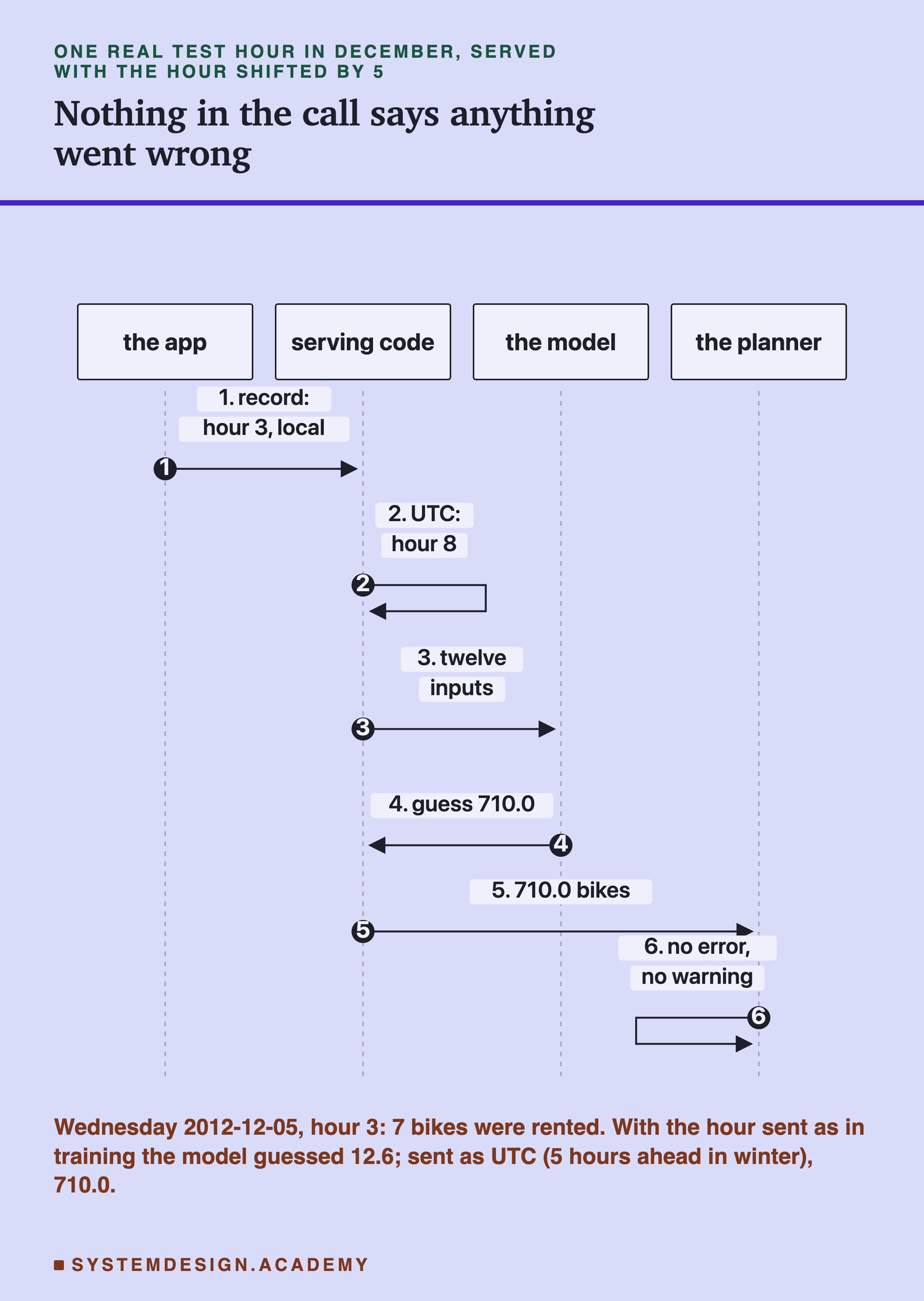
The figure follows one real test hour through a serving call. I picked a December hour on purpose, because in December Washington is exactly 5 hours behind UTC, so here the fixed +5 is real UTC. At 3 in the morning on Wednesday 5 December 2012, 7 bikes were rented. The serving code turned hour 3 into hour 8, the UTC hour, which to the model is the morning rush. It guessed 710.0 bikes. With the hour sent as in training it had guessed 12.6. At every step of that call, something was sent and something came back. There is no step where anything could fail loudly, because nothing did fail. The code ran exactly as written.

The hour skew is the biggest, and the easiest to see, so I start with it. From here on, "shifted by 5" means the main run's fixed +5, which is UTC in winter. The report groups the 3,476 test hours by their real, local hour of the day.

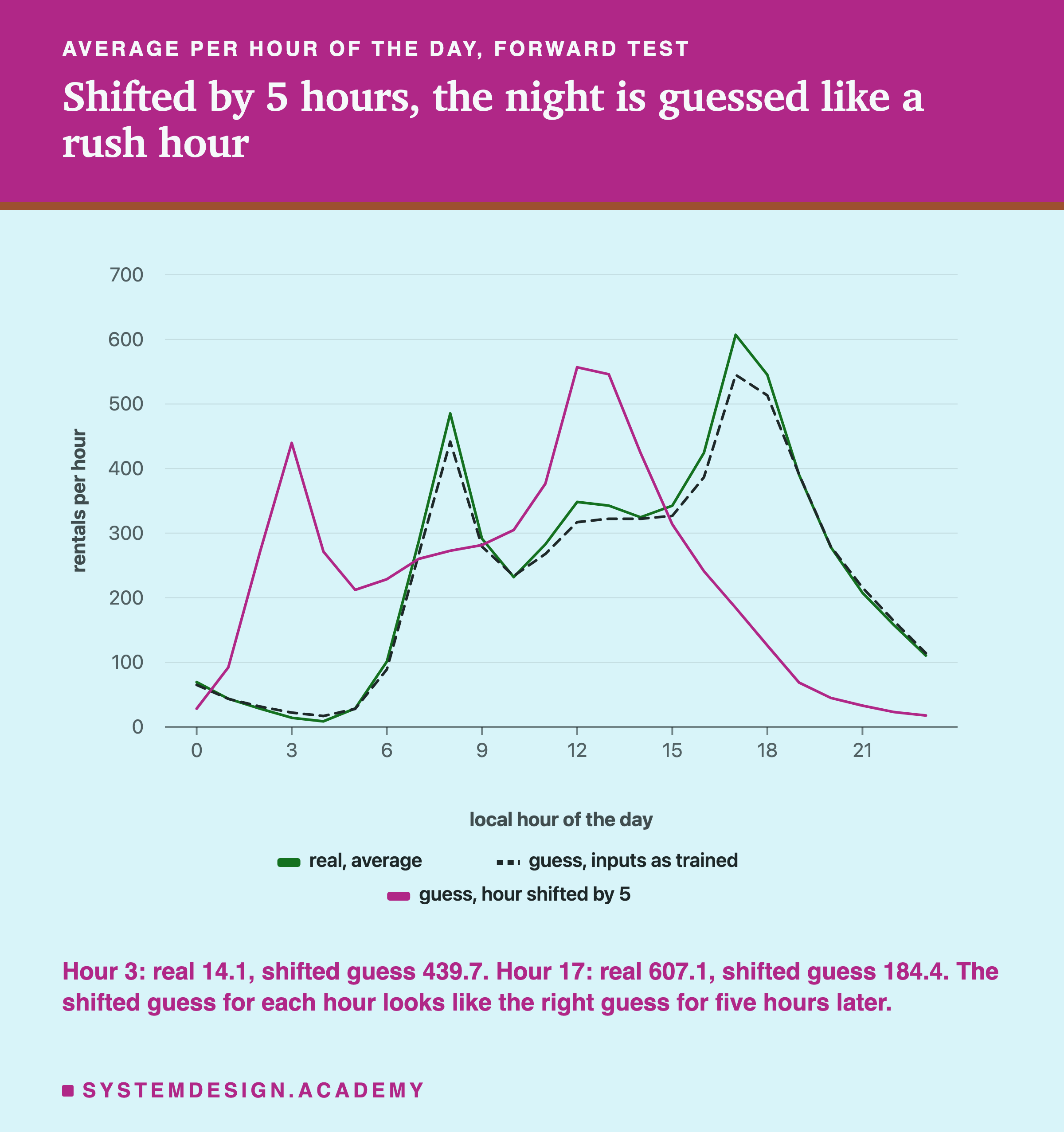
The two lines that move together are the real average count and the guess with the inputs as in training: low at night, a peak for the morning commute at 8, a plateau through the day and a higher peak at 17 and 18. The third line is the guess with every hour shifted by 5. It has the same shape, moved five hours to the left. At local hour 3, when on average 14.1 bikes an hour were rented, the shifted guess averaged 439.7, because the model thought it was 8 in the morning. At local hour 17, the busiest hour, with 607.1 rentals on average, the shifted guess averaged 184.4, because the model thought it was 10 at night.

That is measured, straight from the stored guesses. It also means that the model is not "confused" in any vague way. It answers a precise question correctly: how many bikes are rented at the hour it was told. It was told the wrong hour.

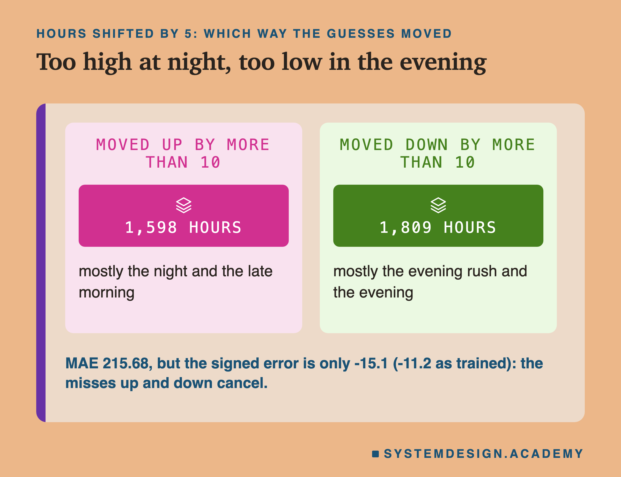
Here is why this matters for how you would watch a model. 1,598 guesses moved up by more than 10 bikes, and 1,809 moved down. The night and the late morning were guessed too high; the evening was guessed too low. The average size of the miss, the MAE, is 215.68. But the signed error, which lets misses in opposite directions cancel, is only -15.1, close to the -11.2 the model had with correct inputs. If the number you watched was "are we guessing too high or too low on average", this skew would be almost invisible, while the model missed by over two hundred bikes an hour.

The two unit skews damage the model in a different way. The hour skew moved values around inside the range the model knew. The unit skews push values outside it.

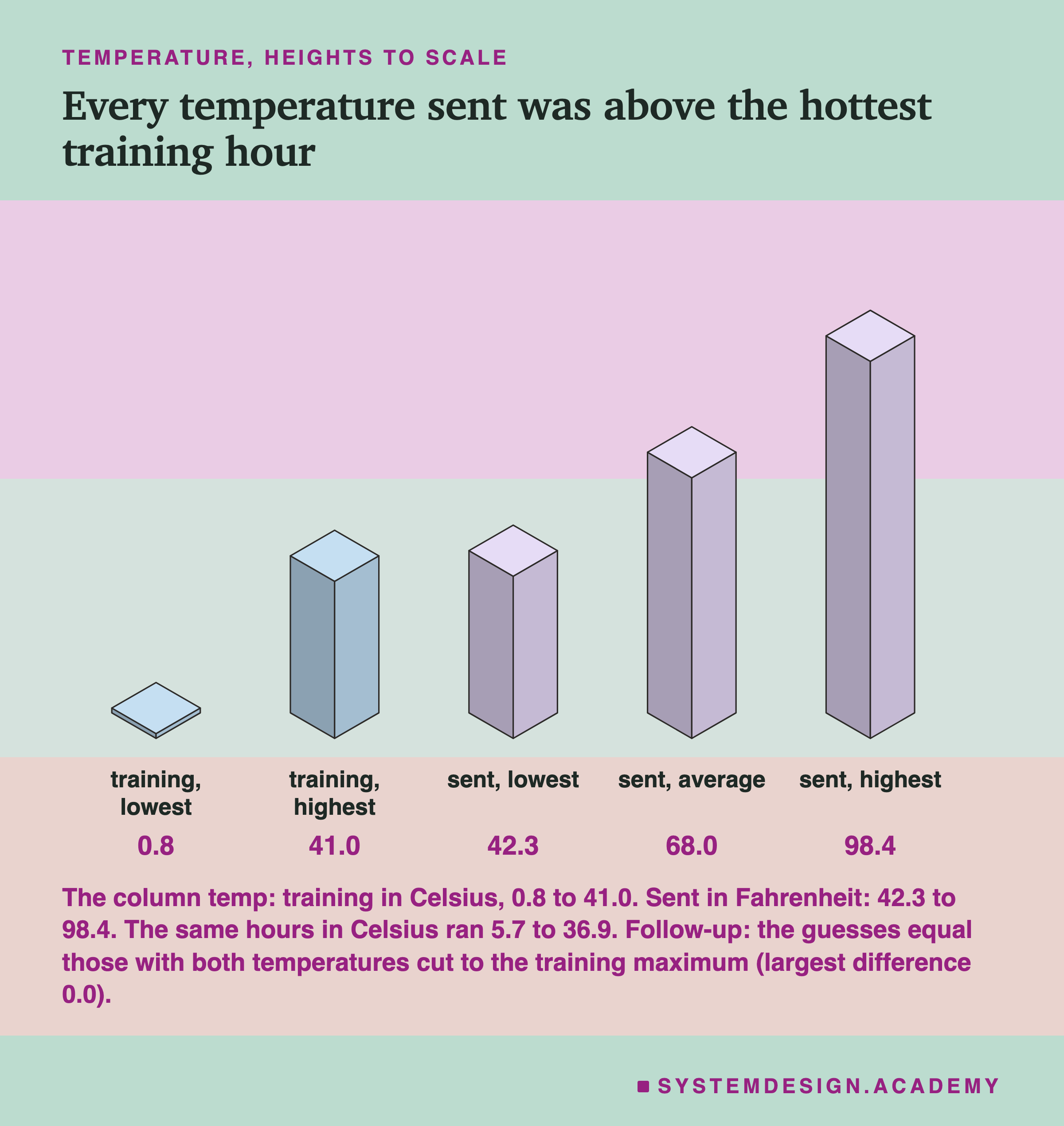
In training, the temp column ran from 0.8 to 41.0 degrees Celsius. The test hours, in Celsius, ran from 5.7 to 36.9: nothing unusual. Converted to Fahrenheit, the same hours ran from 42.3 to 98.4. Every single value sent was above the hottest hour the model had ever seen. The report measures it: 100% of the skewed temp values and 99.1% of the skewed feel_temp values were above the training maximum.

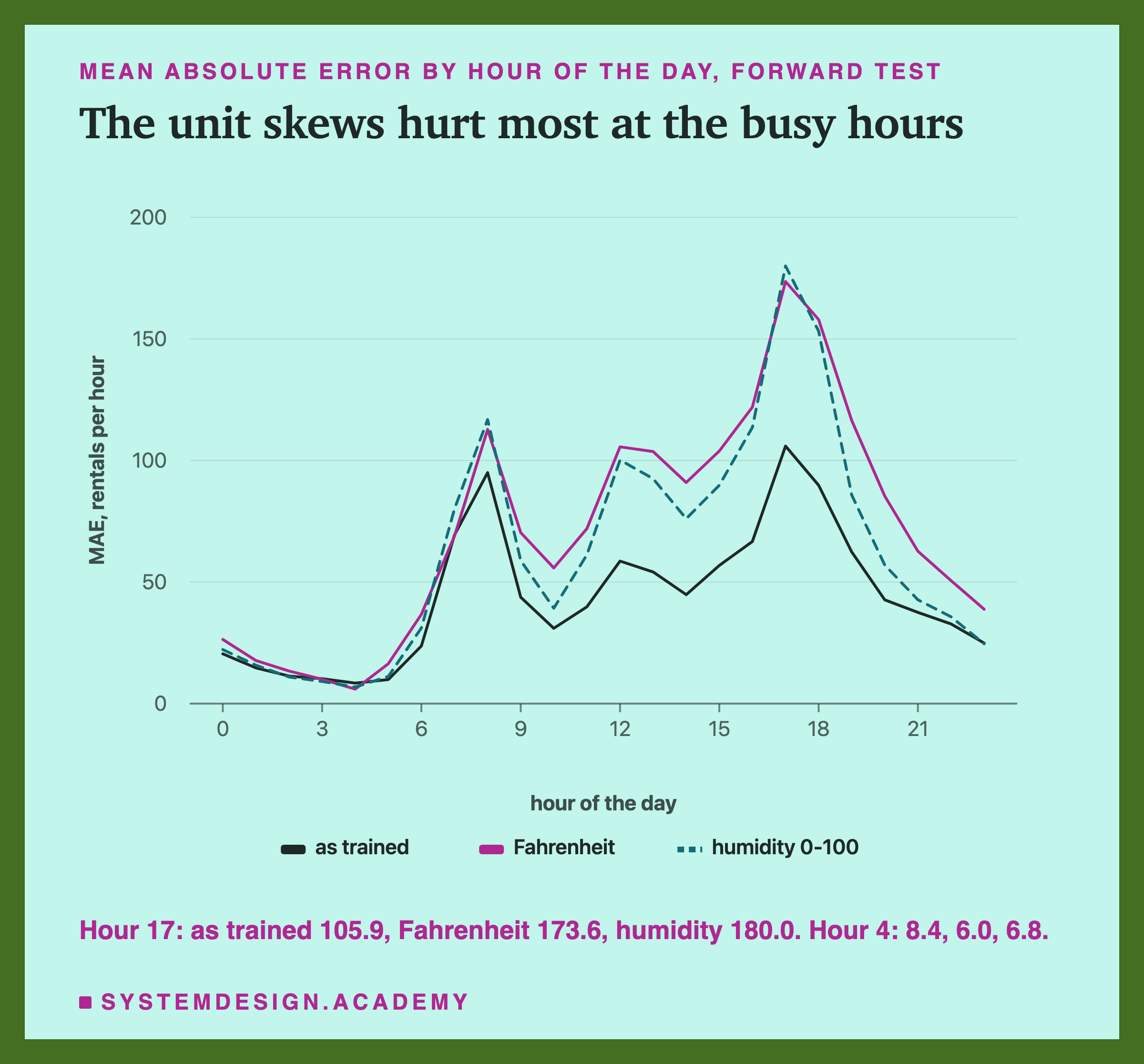
A tree cannot extend what it learned beyond the range it saw. The follow-up measured this directly: sending both temperatures cut down to their training maximum gives exactly the same guesses as sending them in Fahrenheit (the largest difference between the two sets of guesses was 0.0). So to the model, every hour in this skew was simply as hot as the hottest training hour. What is measured is the result: 79.2% of the guesses moved by more than 10 bikes, 1,069 up and 1,684 down, and the MAE rose to 71.84. The biggest damage was at busy hours. At hour 17 the MAE went from 105.9 to 173.6.

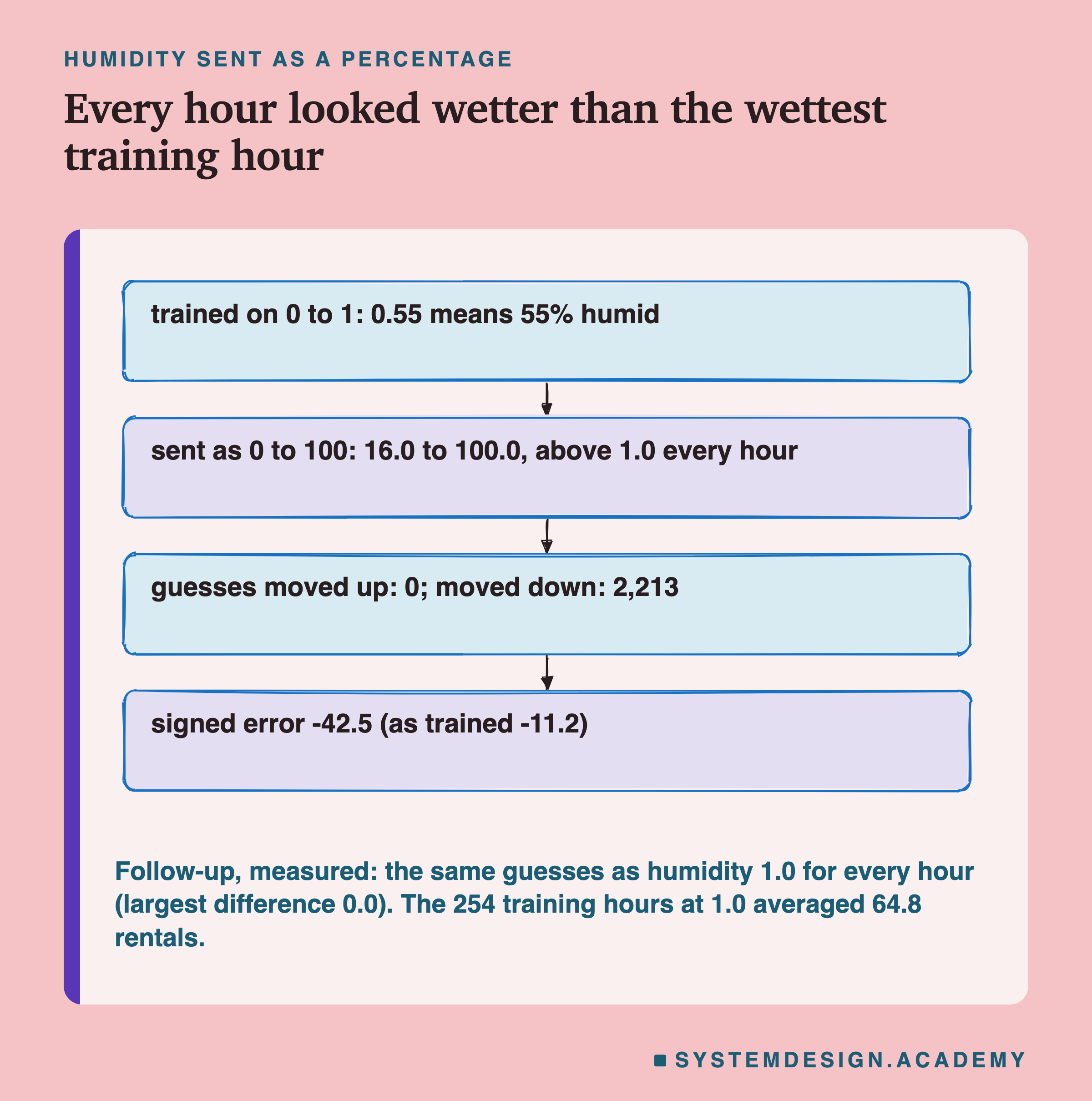
The humidity skew is simpler to read. The model learned humidity as a fraction from 0 to 1, where 0.55 means 55% humid. Sent as a percentage, the test hours arrived as 16 to 100: every hour above the wettest training hour. Not one guess moved up by more than 10 bikes; 2,213 moved down. The signed error went from -11.2 to -42.5: the model now guessed too low almost everywhere. The follow-up measured why: the guesses are exactly the guesses for humidity 1.0 in every hour (largest difference 0.0). The 254 training hours with humidity 1.0 averaged only 64.8 rentals, so to the model every hour now looked like the wettest, quietest hours it had seen.

Of all six skews, only one ever produced an answer that is plainly impossible: a negative number of bikes. The Fahrenheit skew did it 54 times out of 3,476. I read all 54 rows before writing anything about them.

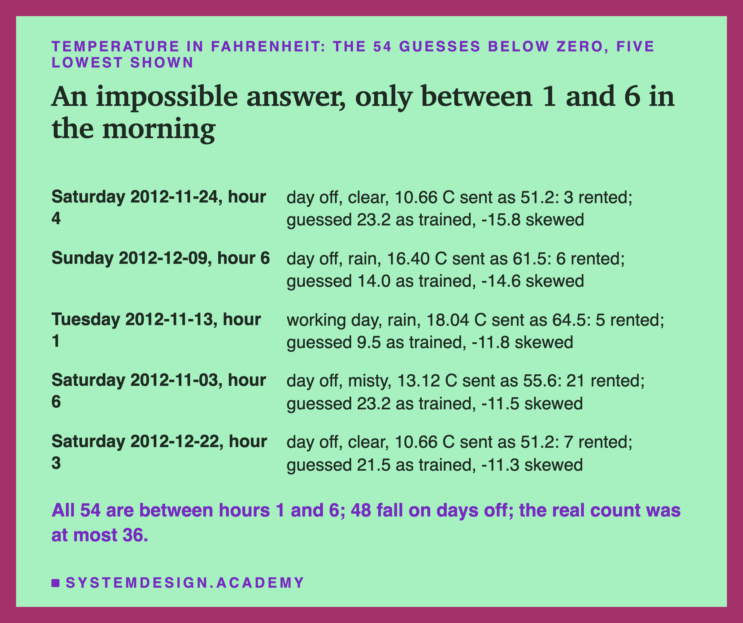
What they share is measured. Every one of the 54 is at an hour between 1 and 6 in the morning; those six hours are 25% of the test. 48 of the 54 are on days off, which are 32% of the test. The real count was small in all of them, at most 36 bikes and 14.6 on average. With the inputs as in training, the model's guesses for these same hours were all positive, at least 7.41. The lowest skewed guess was -15.84, at 4 in the morning on Saturday 24 November 2012, when 3 bikes were rented. The months were spread through the test: 8 in August, 8 in September, 6 in October, 17 in November and 15 in December.

Why below zero? This is a guess, not tested. Boosted trees add up many small corrections, and nothing in them stops the total from going below zero; the training answers were never below 1, but the model does not know that rule. Early mornings on weekends already sit close to zero. An input that no training hour ever had, every hour hotter than the hottest one, seems to have pushed a few of them past it.

This is the one case where a simple sanity check on the output (no negative bike counts) would have noticed something. It would have noticed 54 hours out of 3,476, 1.6%, while 79.2% of the guesses had moved. An output check catches the rare absurd answer, not the common wrong one.

It is natural to ask whether a skew shows up more in some part of the year. The report splits the error by month.

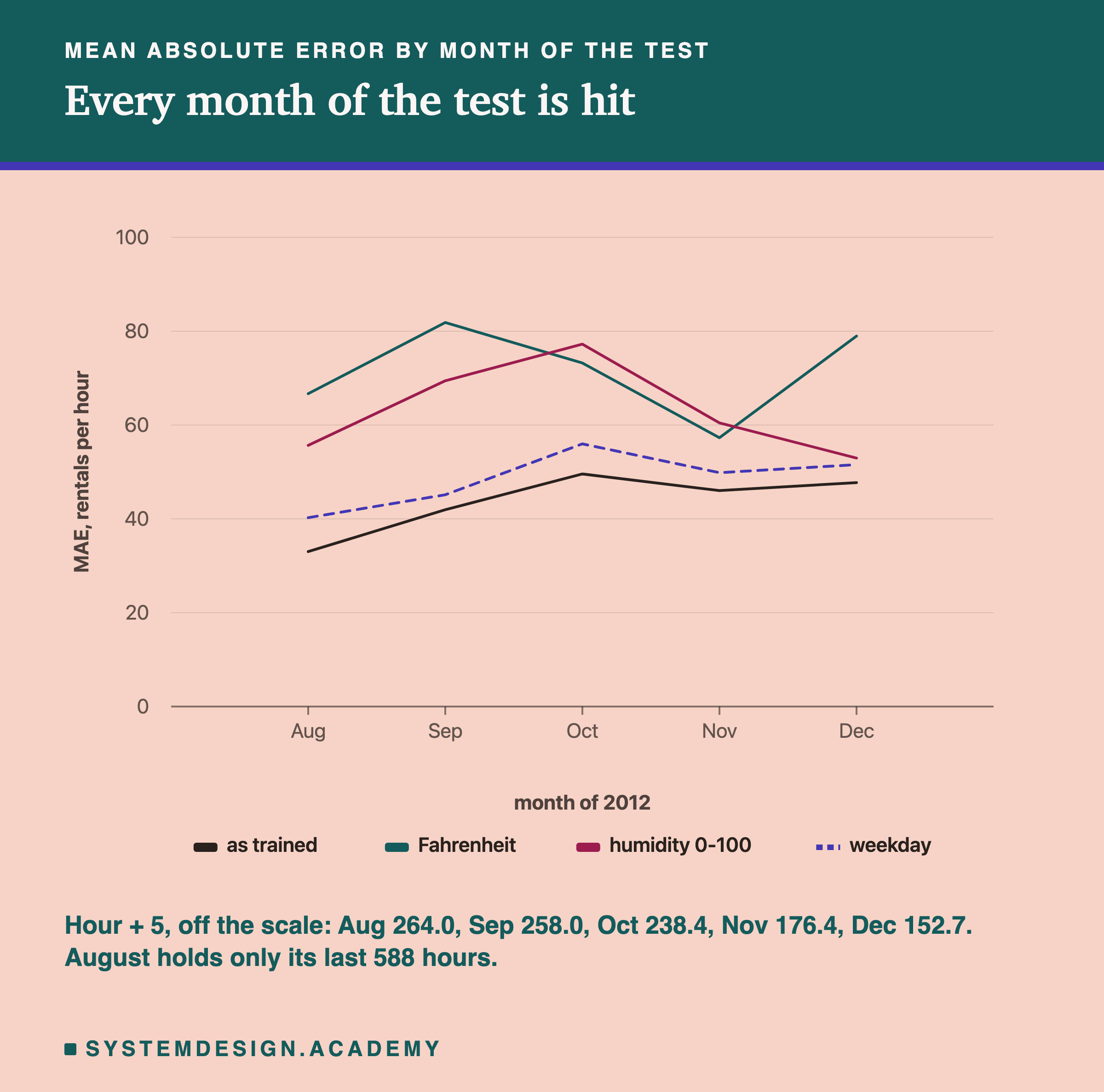
Every skewed line sits above the line for the inputs as trained, in every month of the test. Fahrenheit is between 57.3 (November) and 81.8 (September); humidity between 53.0 (December) and 77.2 (October); the weekday skew between 40.3 and 56.0. The shift by 5 is off the scale of the chart: 264.0 in August, falling to 152.7 in December. It falls roughly in step with how busy each month was: December averaged 166.7 rentals an hour against 290.6 in late August. The report divides each month's MAE by that month's real average, and for the shifted hours it stays between 0.83 and 0.92 in every month. A five-hour shift costs fewer bikes when there are fewer bikes to move.

The practical point is that skew is not a seasonal event. It starts on the day the serving code starts, and it stays until someone fixes the code. Lesson 2's drift built up slowly as the city changed. A skew is at full strength from the first hour.

Now the two skews the average cannot see. The first is the weather label. In training the column held four words: clear, misty, rain and heavy_rain. At serving, a capital letter was added: Clear, Misty, Rain.

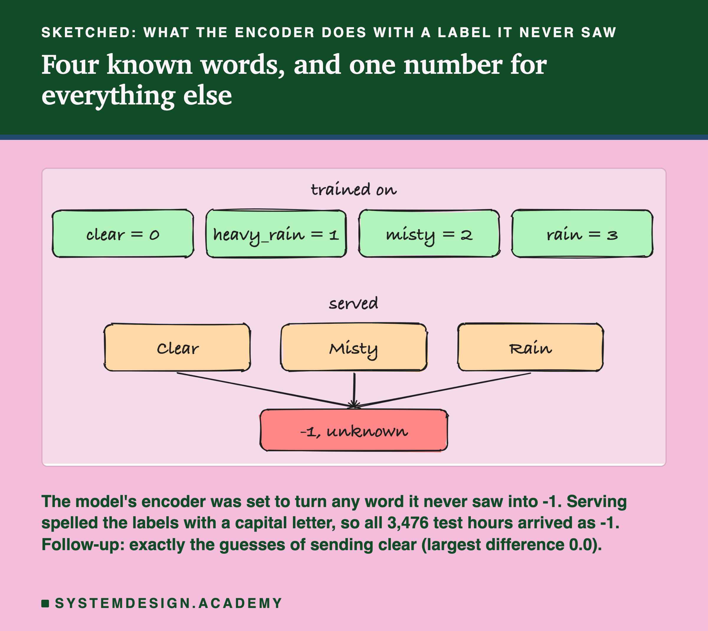
The model reads words through an encoder. The report fits the same kind of encoder on the training rows and prints its codes: clear = 0, heavy_rain = 1, misty = 2, rain = 3. The lab's model was set up, in lesson 1, to turn any word it never saw into -1 instead of crashing. That is a common and sensible setting, and it is exactly why nothing crashed here. The report checks what the three capitalised words become: all three become -1. For the model, every one of the 3,476 hours had the same unknown weather.

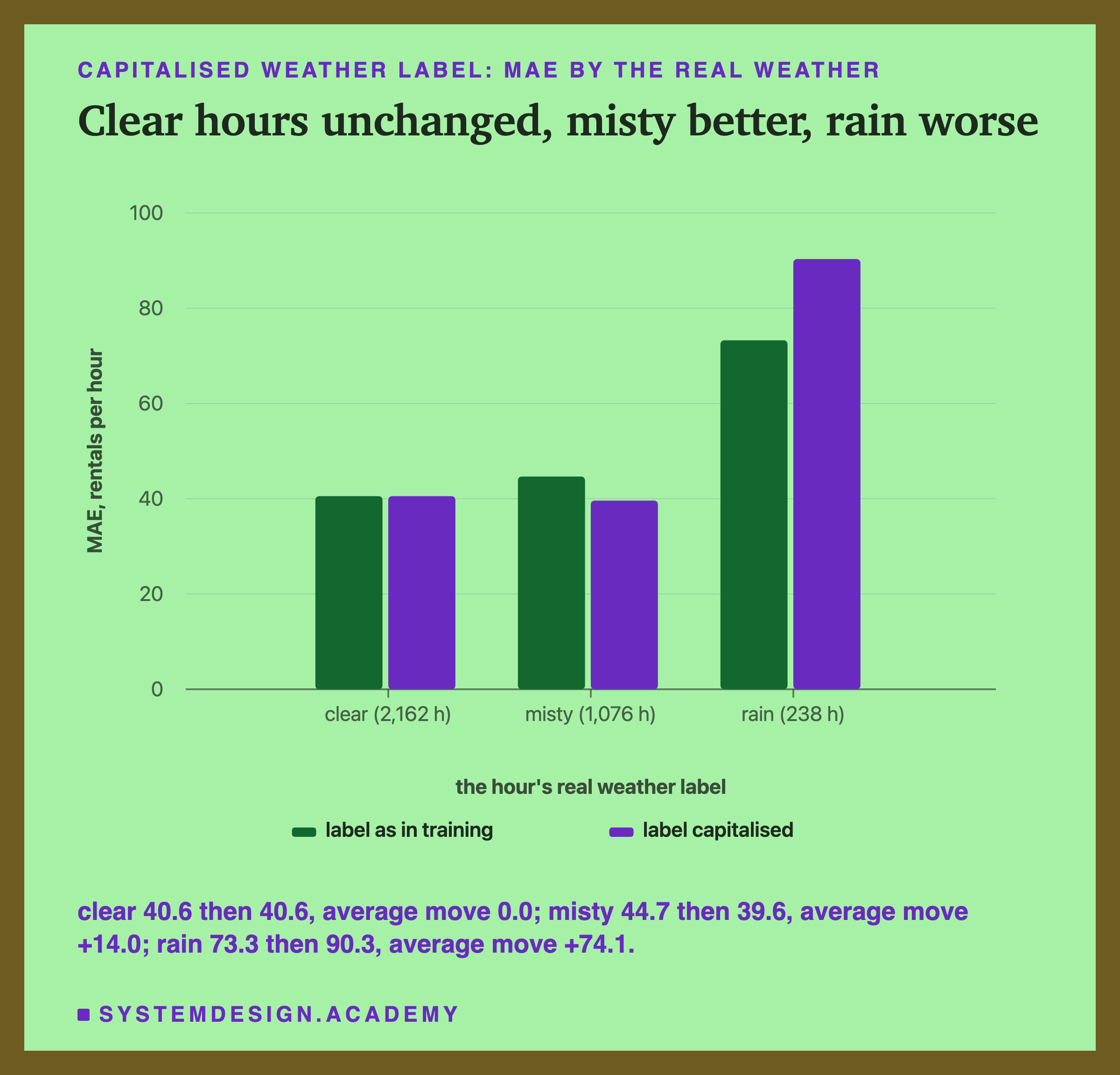
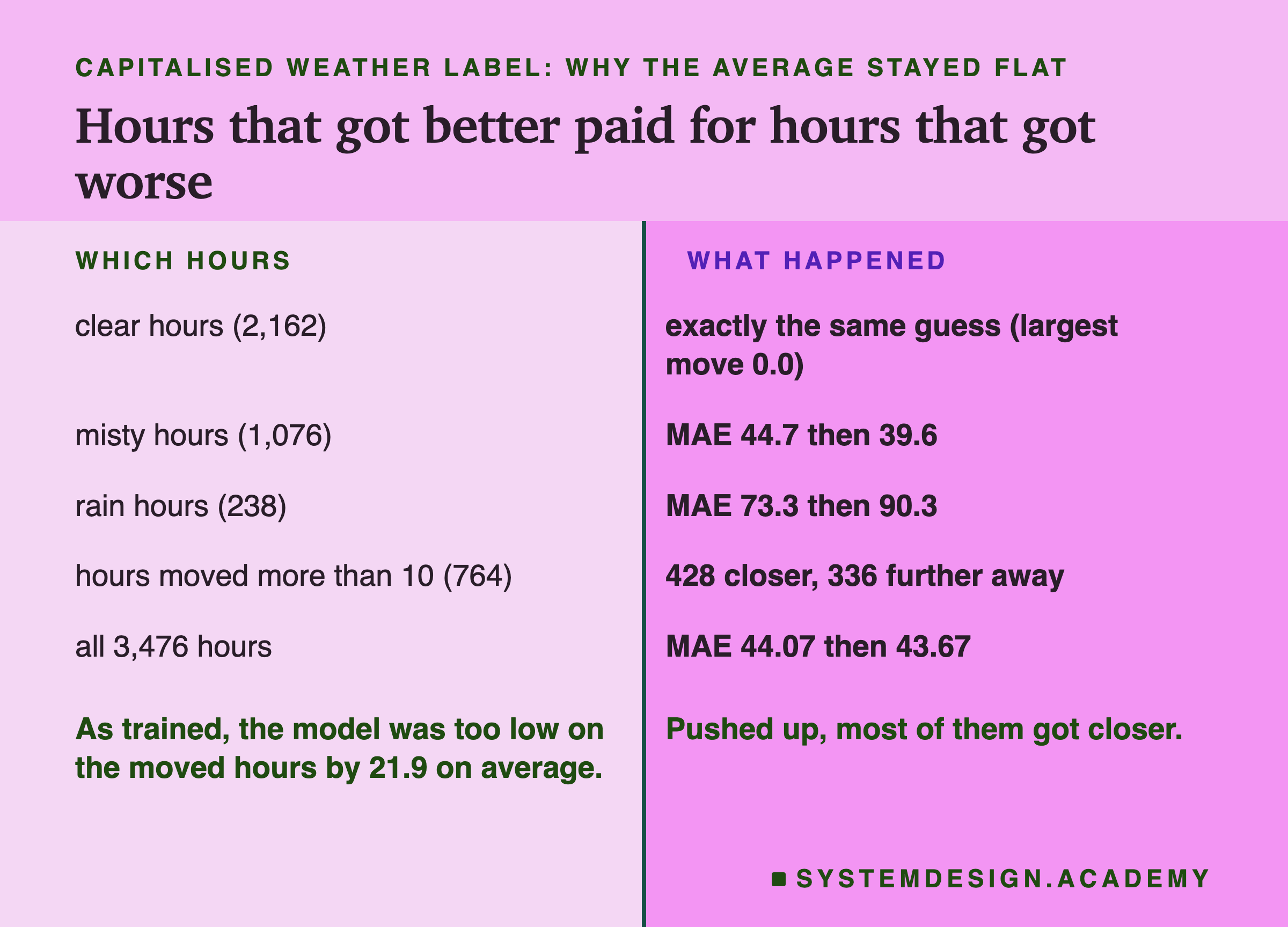
What happened next is measured, by the real weather of each hour. Every clear hour got exactly the same guess as before: the largest change among the 2,162 clear hours was 0.0. Misty hours moved up by 14.0 bikes on average, and rain hours by 74.1. So the model treated the unknown code as if every hour were clear. The follow-up measured this directly: sending the capitalised labels gives exactly the same guesses as sending "clear" for every hour (largest difference 0.0). The reason is simple. Each tree splits the weather code at a few cut points, and any value below its lowest cut goes into its lowest group. -1 is below every code, so it lands in the same group as clear, code 0.

The weekday skew counts days from Monday = 0 instead of the dataset's Sunday = 0. So every real Monday is sent as a Sunday, every Tuesday as a Monday, and so on.

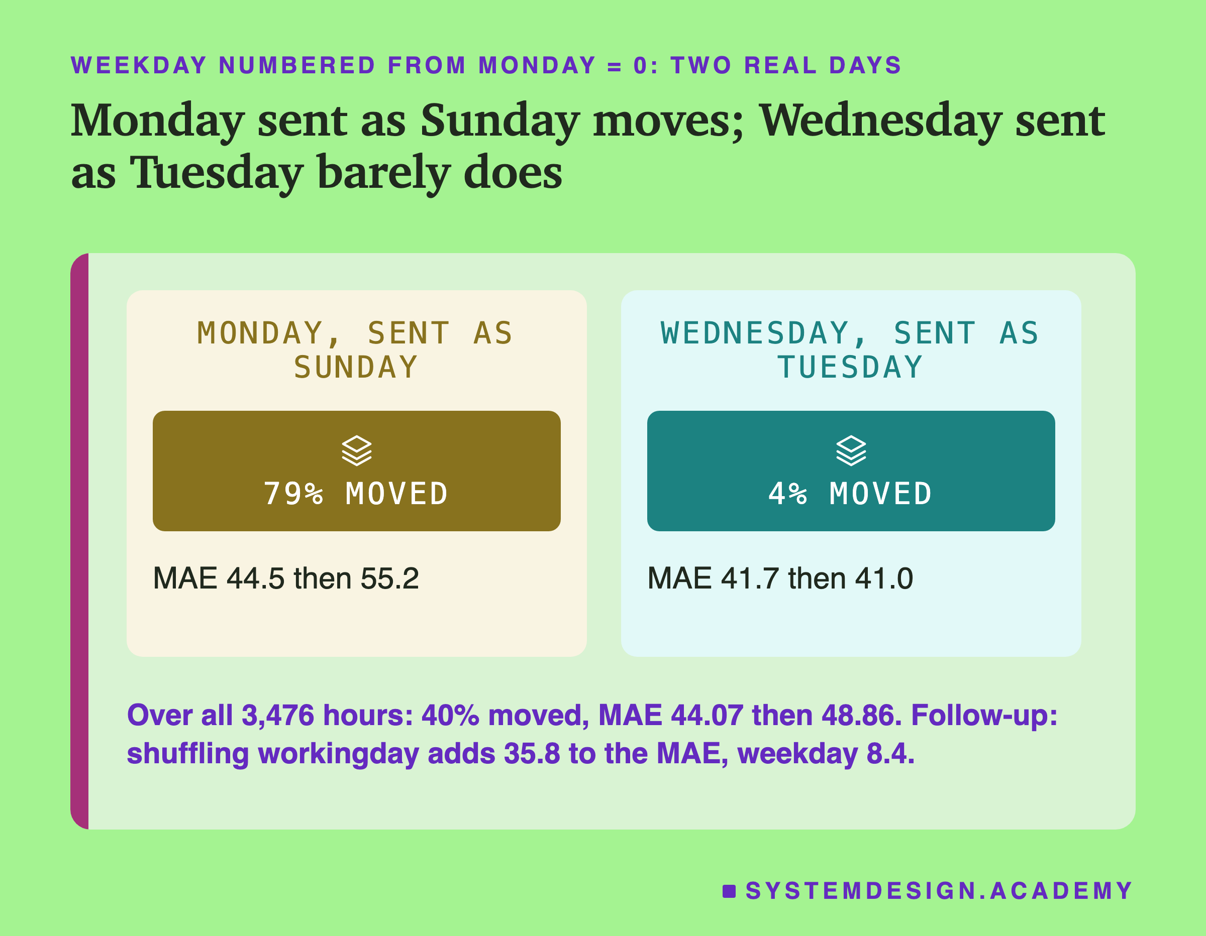
The damage depends on which day is swapped for which. Real Mondays, sent as Sundays, moved a lot: 79% of their guesses changed by more than 10 bikes, and their MAE went from 44.5 to 55.2. Real Wednesdays, sent as Tuesdays, barely moved: 4%, and their MAE went from 41.7 to 41.0. Two ordinary midweek days look alike to the model. A working Monday and a Sunday do not. Real Sundays sent as Saturdays moved 75%, and real Fridays sent as Thursdays 62%. Overall, 40.4% of the guesses moved and the MAE went from 44.07 to 48.86.

It could have been worse. The dataset has a separate working-day column, and that column was still sent correctly. The follow-up measured how much the model leans on each input with permutation importance: shuffle one column's values among the test hours, so that it carries no real information, and see how much the MAE rises. Shuffling the working-day column added 35.8 to the MAE; shuffling the weekday number added only 8.4. (The hour added 156.3, the most of any input, which fits the size of the hour skew.) So the model leans far more on the column that was still correct.

The missing wind speed is the quietest skew. In training, 11.8% of the hours already had a wind speed of exactly 0: calm hours are real. So a serving default of 0 is a value the model knows well. Hours whose real wind was 0 got exactly the same guess (the largest change was 0.0). Windier hours moved: of the 363 test hours with a wind speed of 20 or more, 34% moved by more than 10 bikes. Overall 7.8% moved, 263 up and 7 down, and the MAE ended at 43.69 against 44.07. Again the average cannot see it, and again there is a real change underneath: the model now believes every hour is calm.

An average hides single hours, so the report also lists, for each skew, the hours whose miss grew the most compared with the inputs as trained. The dates are rebuilt from the weekday column exactly as in lesson 1, and I chose this table after seeing the results.

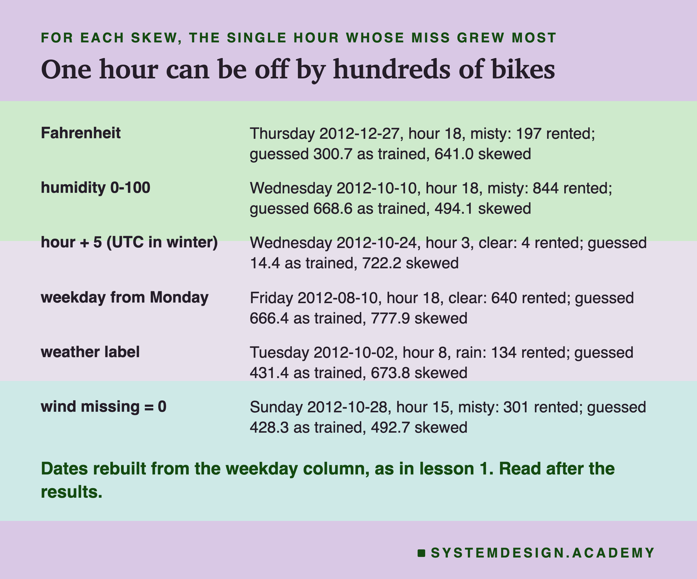
The worst hour for the shift by 5 is 3 in the morning on Wednesday 24 October: 4 bikes rented, a guess of 722.2. In October, real UTC would have been hour 7, not 8, so this exact miss belongs to the fixed shift; the December hour on the serving-call slide is the same kind of miss with real UTC. The worst Fahrenheit hour is 6 in the evening on Thursday 27 December 2012, a misty winter evening with 197 rentals. As trained, the model guessed 300.7; with the temperature in Fahrenheit, it guessed 641.0, which looks like a summer evening. The worst humidity hour went the other way: 6 in the evening on 10 October, 844 bikes rented, guessed 668.6 as trained and 494.1 with humidity as a percentage.

The worst weather-label hour is a rainy 8 in the morning on 2 October: 134 rented, guessed 431.4 as trained and 673.8 with the label capitalised. That is the capitalised label at its worst: a rainy rush hour read as a clear one. Even the quietest skew has a bad hour: with the wind speed filled with 0, a misty Sunday afternoon in October went from a guess of 428.3 to 492.7, against 301 real rentals.

These are single hours from one run. They are here because in production someone sees single hours: a planner sends trucks, a shop orders stock, a person makes a decision on one number.

If the model cannot tell you about skew and the average error cannot, the only place left to look is the inputs themselves. The next lesson is about checks. This slide only measures what those checks would have to work with: each skewed input in training, and what serving sent.

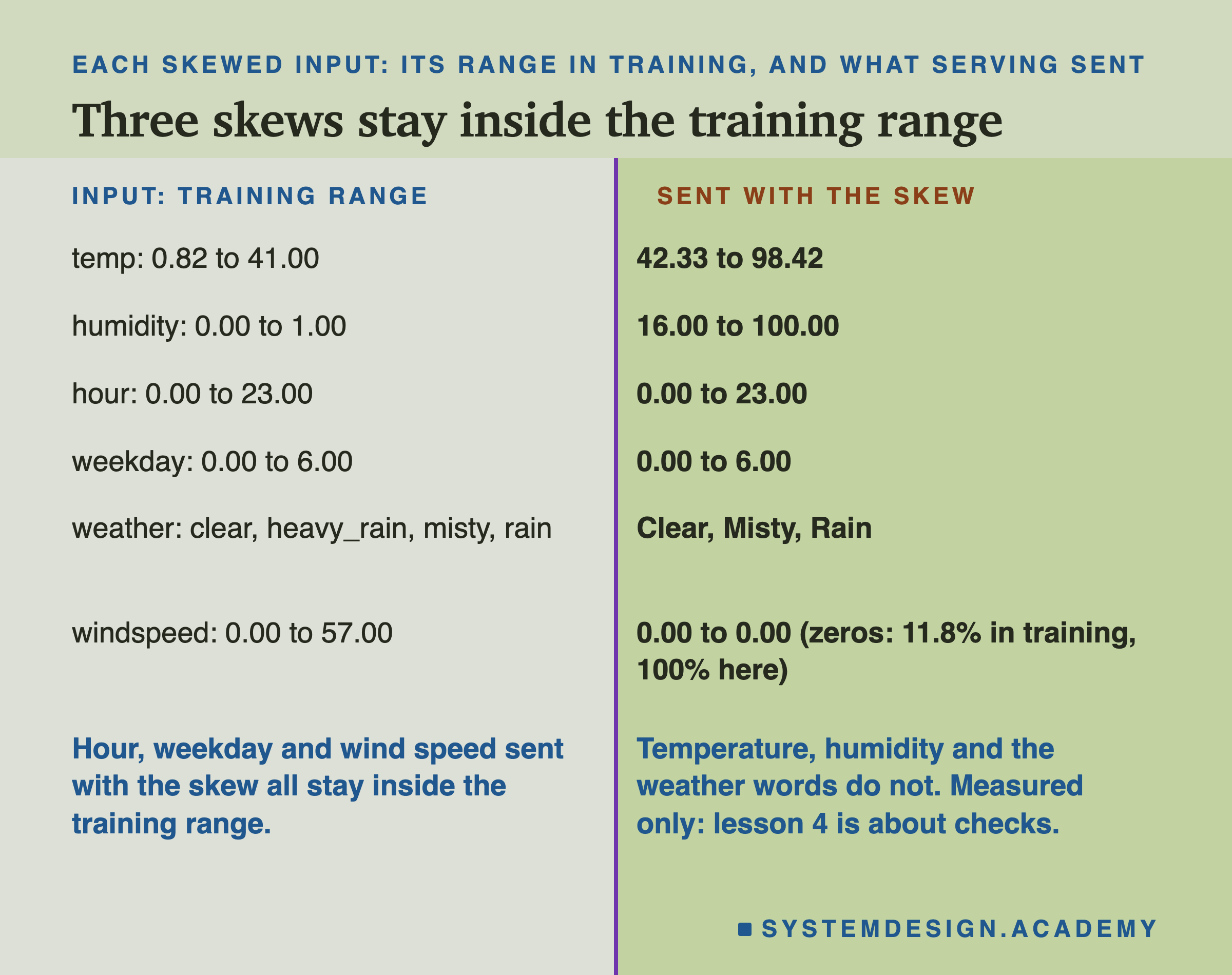
Three skews send values the training data never held. Temperature in Fahrenheit ran from 42.33 to 98.42 against a training range of 0.82 to 41.00. Humidity as a percentage ran from 16 to 100 against 0 to 1. The capitalised labels are words the training data never contained.

The other three stay inside the training range. The shifted hour still runs from 0 to 23. The shifted weekday still runs from 0 to 6. The wind speed filled with 0 is inside 0 to 57. The report goes one step further for the hour and the weekday: it compares how often each value appears. With correct inputs, the share of any single hour differed by at most 0.1 points between training and serving; with the shifted hours, 0.2. (A point here is one percentage point: 5% against 5.1% is 0.1 points.) For the weekday it was 0.6 either way. Shifting every hour by five keeps almost the same mix of hours, because the test covers almost whole days: it starts at noon on 7 August and a few hours are missing. So the biggest skew in the lab, 4.89 times the error, is the one whose inputs look the most normal one column at a time.

I stop at measuring here. Which checks catch which break, and how often they raise an alarm when nothing is wrong, is lesson 4.

This script is the lab made small. It downloads the same data, trains the boosted trees once, and sends the test hours four times: as in training, with every hour shifted by 5 (the script calls this utc_hours and its comment says UTC, which is true only in winter, as the results slide explains), with temperatures in Fahrenheit, and with the weather label capitalised. It does not need a GPU.

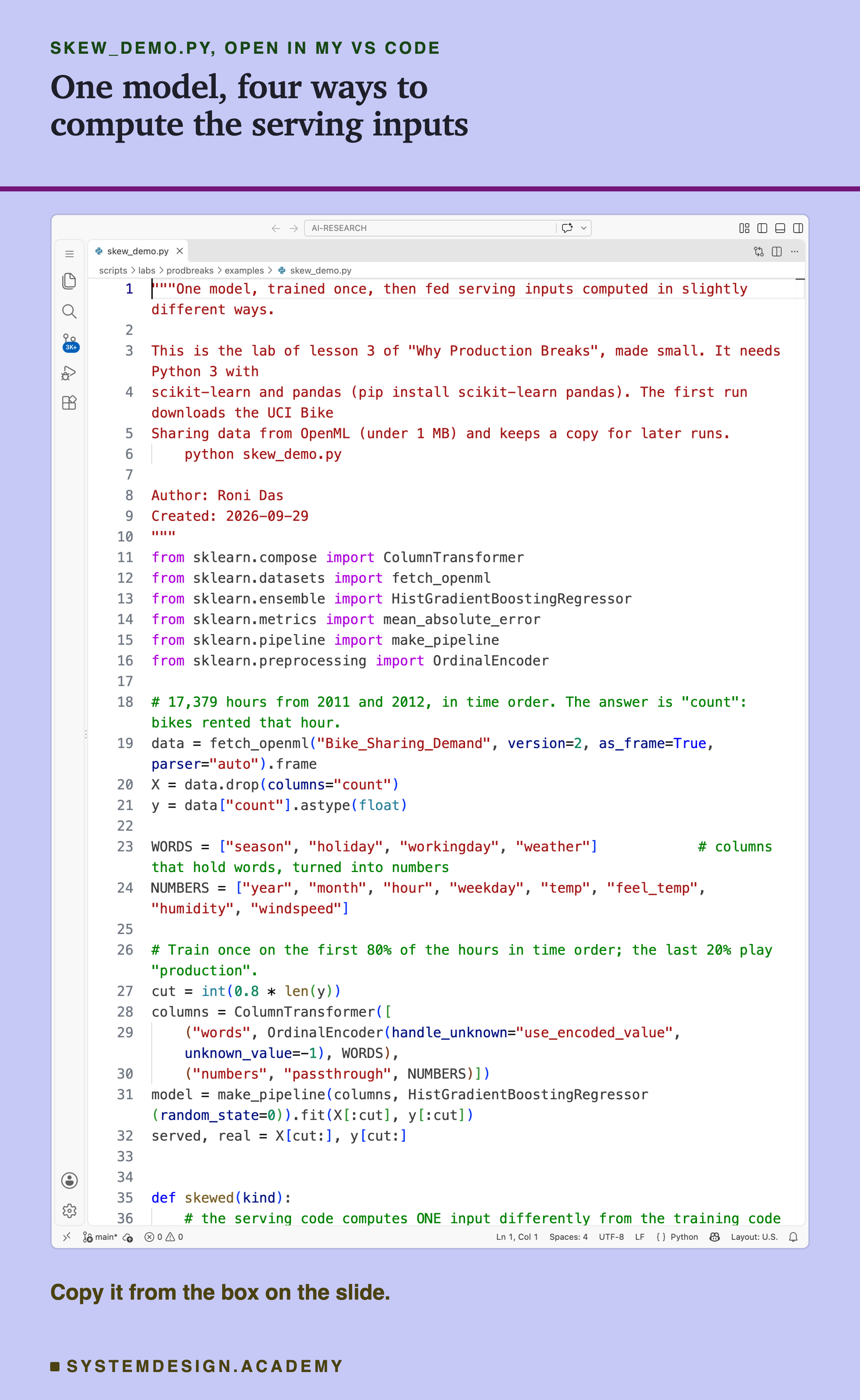
Before you run this lab. You need Python 3 and two libraries: pip install scikit-learn pandas. scikit-learn holds the model, the encoder, the score and the download; pandas holds the table. The first run downloads the Bike Sharing data from OpenML, so it needs an internet connection once; scikit-learn keeps a copy in a folder in your home directory (scikit_learn_data) for later runs. I ran it with scikit-learn 1.9.1 on a Mac. scikit-learn runs the same way on Windows and Linux, but I have not checked the numbers there, and another version of scikit-learn may give slightly different decimals.

"""One model, trained once, then fed serving inputs computed in slightly different ways.

This is the lab of lesson 3 of "Why Production Breaks", made small. It needs Python 3 with
scikit-learn and pandas (pip install scikit-learn pandas). The first run downloads the UCI Bike
Sharing data from OpenML (under 1 MB) and keeps a copy for later runs.
    python skew_demo.py

Author: Roni Das
Created: 2026-09-29
"""
from sklearn.compose import ColumnTransformer
from sklearn.datasets import fetch_openml
from sklearn.ensemble import HistGradientBoostingRegressor
from sklearn.metrics import mean_absolute_error
from sklearn.pipeline import make_pipeline
from sklearn.preprocessing import OrdinalEncoder

# 17,379 hours from 2011 and 2012, in time order. The answer is "count": bikes rented that hour.
data = fetch_openml("Bike_Sharing_Demand", version=2, as_frame=True, parser="auto").frame
X = data.drop(columns="count")
y = data["count"].astype(float)

WORDS = ["season", "holiday", "workingday", "weather"]            # columns that hold words, turned into numbers
NUMBERS = ["year", "month", "hour", "weekday", "temp", "feel_temp", "humidity", "windspeed"]

# Train once on the first 80% of the hours in time order; the last 20% play "production".
cut = int(0.8 * len(y))
columns = ColumnTransformer([
    ("words", OrdinalEncoder(handle_unknown="use_encoded_value", unknown_value=-1), WORDS),
    ("numbers", "passthrough", NUMBERS)])
model = make_pipeline(columns, HistGradientBoostingRegressor(random_state=0)).fit(X[:cut], y[:cut])
served, real = X[cut:], y[cut:]


def skewed(kind):
    # the serving code computes ONE input differently from the training code
    z = served.copy()
    if kind == "utc_hours":                                       # hour in UTC, not local time
        z["hour"] = (z["hour"] + 5) % 24
    elif kind == "fahrenheit":                                    # degrees Fahrenheit, not Celsius
        z["temp"] = z["temp"] * 9 / 5 + 32
        z["feel_temp"] = z["feel_temp"] * 9 / 5 + 32
    elif kind == "weather_label":                                 # "Clear" where training saw "clear"
        z["weather"] = z["weather"].astype(str).str.capitalize()
    return z


baseline = model.predict(served)
for kind in ["none", "utc_hours", "fahrenheit", "weather_label"]:
    guess = model.predict(skewed(kind))
    moved = (abs(guess - baseline) > 10).mean()
    print(f"{kind:<14} MAE {mean_absolute_error(real, guess):6.2f}   "
          f"moved more than 10 bikes {100 * moved:5.1f}%   lowest guess {guess.min():6.1f}")

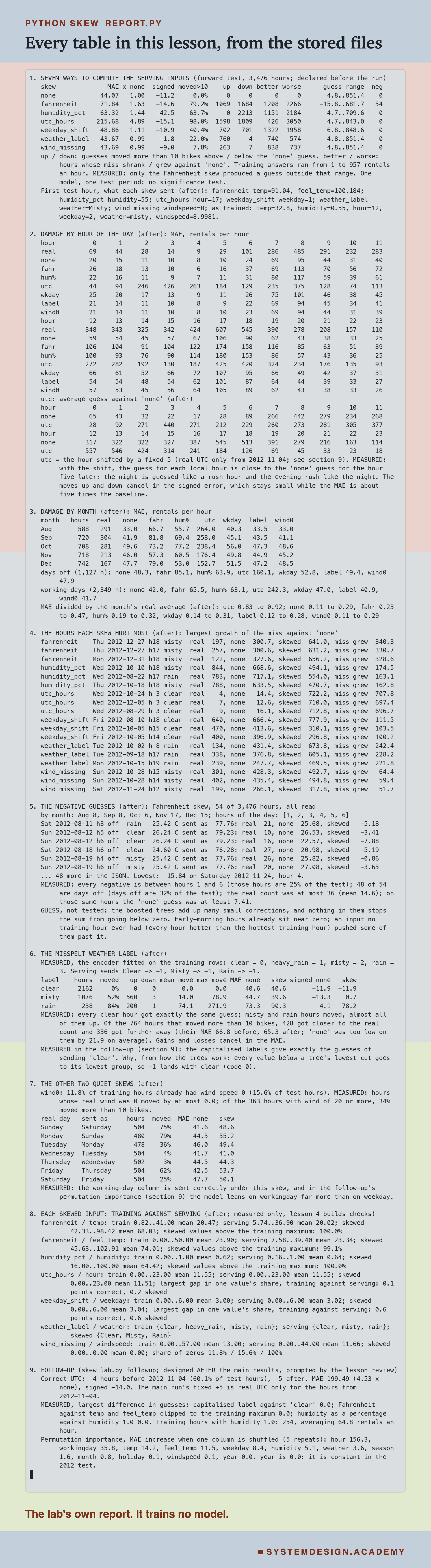
The report lives in scripts/labs/prodbreaks/skew_report.py. It reads the lab's stored results, results/skew.json, and the Bike Sharing data itself from scikit-learn's local copy, for the hour, month, weekday and weather of each test hour. It trains no model. The only thing it fits is an encoder on the training rows' weather column, to print the codes; an encoder only lists the words it has seen.

Before it prints anything, it checks the files against each other. The stored real counts must be the counts in the data, row for row. Each condition's MAE, signed error, moved share and negative count are computed again from the stored guesses and must match the stored scores. The "none" guesses must be exactly lesson 1's stored forward guesses. The rebuilt dates must agree with every row's month and weekday. If anything differs, the report stops.

What came before the run, in skew_lab.py: the model, the test, the seven conditions and the five numbers per condition. What came after I saw the results: the tables by hour, month and working day, the direction of the moves, the hours that got better or worse, the worst hours, the reading of the negative guesses, the encoder codes, the weather, weekday and wind breakdowns, and the ranges in training against serving. Section 9 reads the follow-up, skew_lab.py followup, which was designed after the main results and prompted by a review of this lesson: the correct UTC offset, the three mechanisms tested directly, and the permutation importance. Every explanation line in the report says MEASURED or GUESS.

This box has no model in it. It holds the 3,476 forward test hours in time order (the month, the hour, whether it was a working day, the weather and the real count) and the lab model's stored guess for each hour under each of the seven conditions. It runs in your browser.

As it is, the box prints each condition's MAE and the share of guesses that moved by more than 10 bikes. The guesses are stored to one decimal here, so a few of the last digits differ slightly from the lesson: Fahrenheit prints 71.83 instead of 71.84, and the moved shares for humidity, the weekday, the label and the wind print 63.6%, 40.3%, 21.8% and 7.7% instead of 63.7%, 40.4%, 22.0% and 7.8%.

Try by_hour("utc_hours") to see the five-hour shift hour by hour, or by_month("fahrenheit"). The functions take a rule for which hours to keep, so you can cut the test your own way: mae("weather_label", lambda i: WEATHER[i] == "r") against mae("none", lambda i: WEATHER[i] == "r") shows the rain hours getting worse, and the same with "m" shows the misty hours getting better. moved("weekday_shift", lambda i: WORKING[i] == "0") gives the share of days-off hours that moved. Every number is from the real guesses of the lab's model.

Loading. fetch_openml("Bike_Sharing_Demand", version=2, as_frame=True) downloads the data (or reads the local copy) as a pandas table. X is the 12 input columns and y is count, the answer.

Training once. The model is the same pipeline as in lessons 1 and 2: a ColumnTransformer that turns the four word columns into number codes with an OrdinalEncoder and passes the eight number columns through, followed by HistGradientBoostingRegressor(random_state=0). The setting handle_unknown="use_encoded_value", unknown_value=-1 is what makes the encoder turn a word it never saw into -1 instead of raising an error. It is trained once, on X[:cut], the first 80% of the hours. Nothing in the script trains it again.

The skew. skewed(kind) copies the test inputs and changes one column: (hour + 5) % 24 for the shift by 5 (the % 24 wraps hour 23 + 5 around to hour 4), x * 9 / 5 + 32 for Fahrenheit, and .str.capitalize() for the label. This function stands for the serving code. In a real system it would be a separate program; here it is a few lines, which is the point: the difference between correct and skewed inputs is one line.

This lab measured damage. It did not test any fix, so what follows is advice, the usual practice in teams that run models in production, not something these numbers prove.

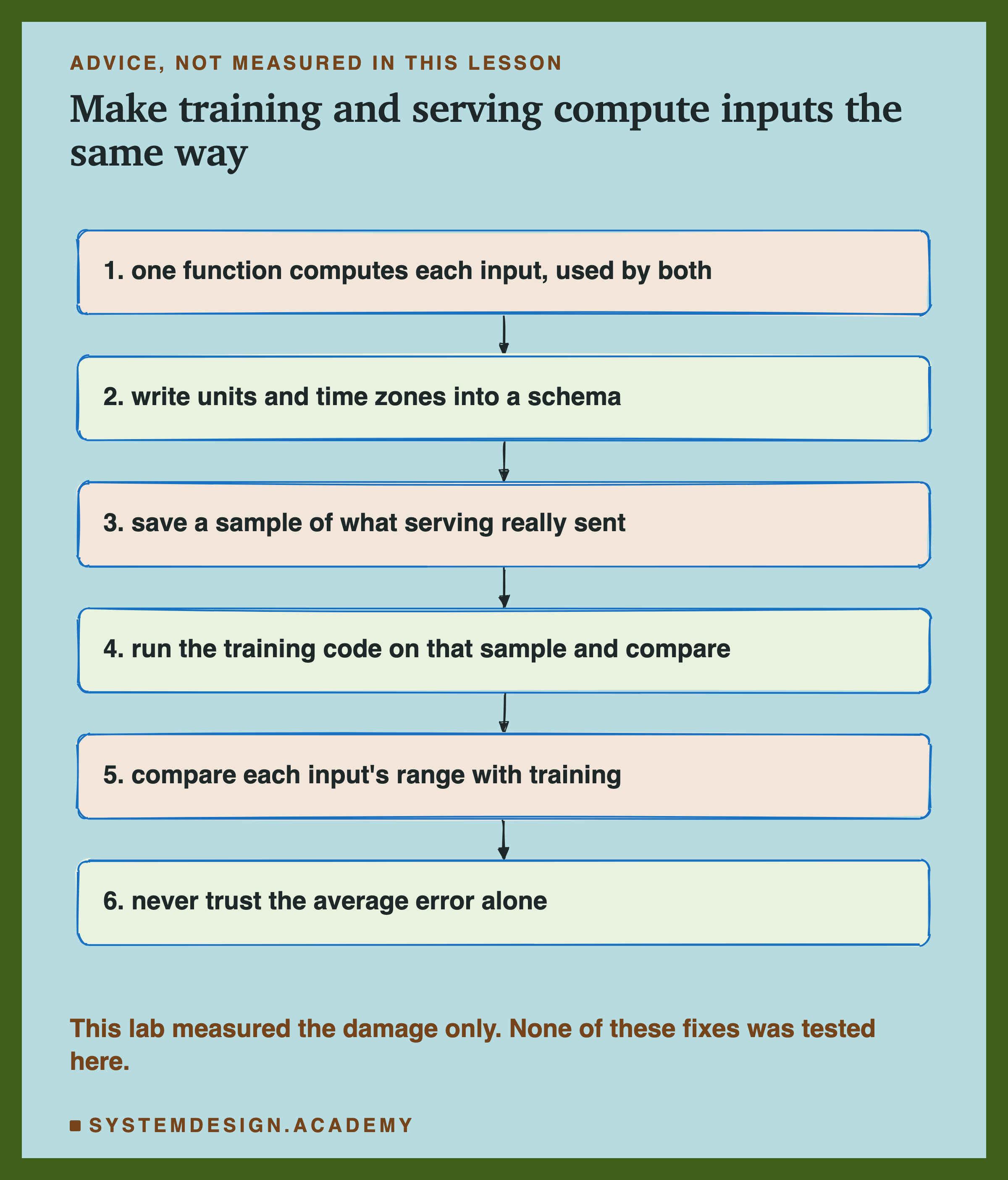
Share one code path. The strongest fix is to have no second piece of code at all. Write each input once, as a function, and call that same function when you build the training data and when you serve. Many teams keep these functions in one shared library or a feature store, a system that computes and stores inputs so that training and serving read the same values. If the serving system is in another language, generate both from one definition, or at least run both on the same records in a test.

Pin units and time zones in a schema. A schema is a written description of each input: its name, its type, its unit, its allowed range or allowed words, its time zone. "temp: float, degrees Celsius, expected -10 to 45." "hour: integer 0 to 23, local time, America/New_York." A schema turns an unwritten assumption into something code can check.

Decide what unknowns and missing values mean. An encoder that turns unknown words into -1 kept the service running here, which is good, and it hid the problem, which is not. Count how often it happens. The same for defaults: if training dropped rows with no wind reading and serving fills 0, the two agree on nothing.

Compare training and serving inputs. Save a sample of what serving really sends. Run the training code on the same raw records and compare the two, value by value. Then compare each input's values at serving with its values in training: ranges, the words that appear, how often each value appears. The ranges slide showed that this catches some skews and not others. Lesson 4 measures which.

Never trust the average error alone. The capitalised label and the missing wind speed left it flat. Look at the error by slice (by hour, by weather, by kind of day), and look at how much the guesses themselves moved after any change to the serving code.

It matters most when training and serving are different code. A model trained in a notebook on a database export and served from a web service written by another team is the classic case. So is a model fed by a third-party data provider, or one whose inputs come from devices with their own settings. Here, one line in that second piece of code moved the error from 44.07 to 215.68.

It matters when inputs have units, clocks or words. Temperatures, money, distances, timestamps, day and month numbers, and anything the model reads as a word. Every one of those has more than one reasonable way to be written, and the lab broke each kind.

It matters when the answers arrive late. For bike rentals, the real count is known one hour later, so a bad error shows up quickly, at least if you look at it by slice. When the real answer arrives weeks later (a loan repaid, a customer who leaves), a skew can run for a long time before any error can be measured at all. There, comparing inputs is the only early warning.

It matters less when one pipeline does everything. If the exact same function computes each input for training and serving, from the same kind of raw record, most of these skews cannot happen. That is why the first piece of advice is to share one code path.

It is not the same as drift. In lesson 2 the world changed and the inputs honestly described a new world. Retraining helped there, through the year input: lesson 2's follow-up found that without the year column, retraining barely helped. Here the world did not change; the description did. Retraining a model on skewed inputs would teach it the skew, and it would break again the day someone fixes the serving code. The fix for skew is in the code, not in the model.

Not a reason to panic about every small change. The wind default moved 7.8% of the guesses and the weekday numbering 40.4%, with very different costs. Measure the change before you decide how urgent it is, the way this lab did.

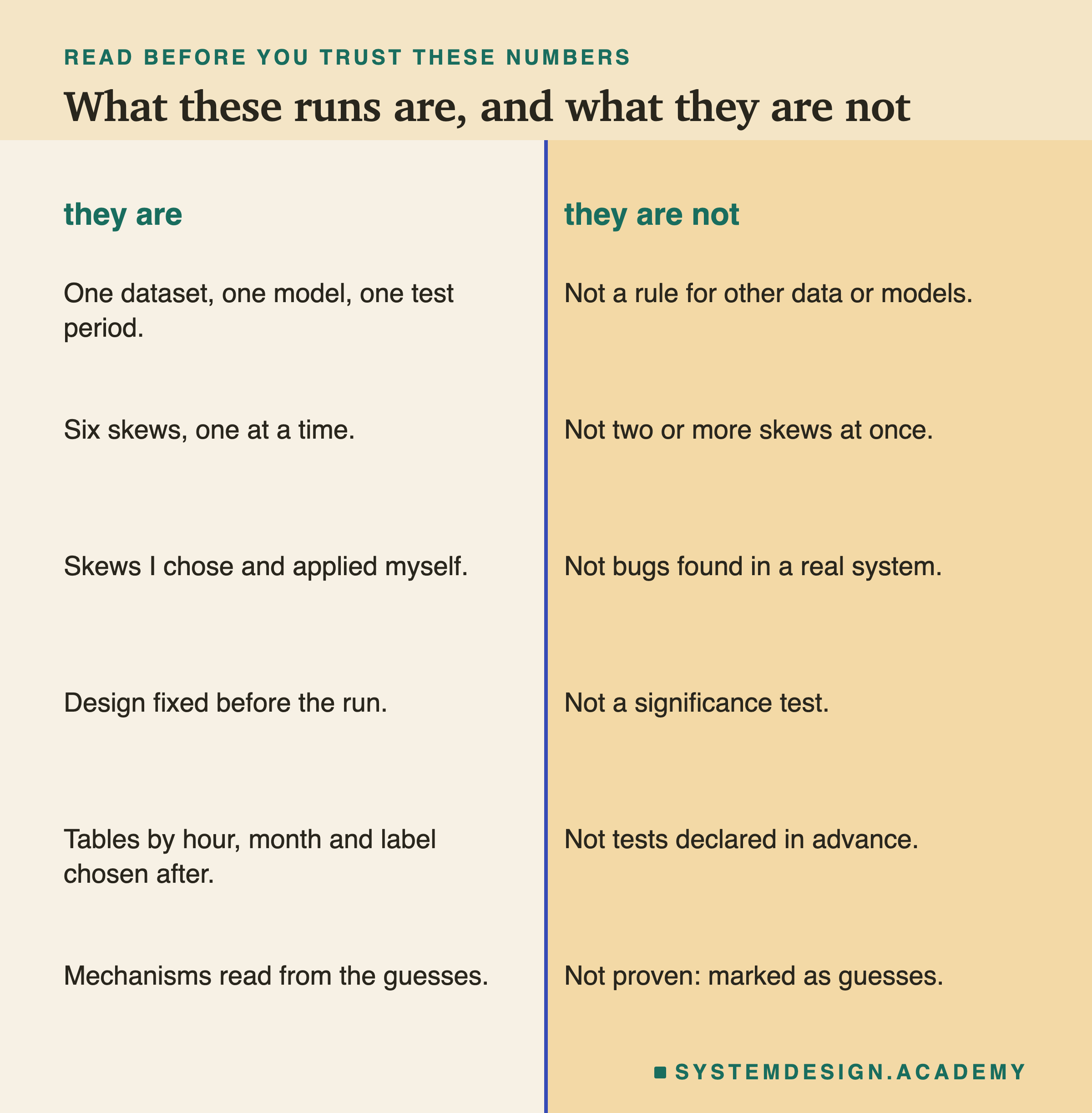
One dataset, one model, one test period. Hourly bike rentals in one city, boosted trees with default settings, the last 20% of the hours. Another model would react to the same skews differently. A linear model, for example, cannot keep every value above the training range at one level the way trees do; it would carry on the line, and could produce much larger or much smaller numbers. I did not run one.

Six skews, one at a time, chosen by me. Real systems can have several at once, and they can interact. These six are realistic kinds of skew, but they are not bugs found in a real bike system. The fixed +5 hours is real UTC only from 4 November; the follow-up with the correct offset gave 199.49 instead of 215.68.

No significance test. The lab declared none, and one model on one test period cannot support one. That is why the lesson never says the capitalised label or the missing wind speed "improved" the model: 43.67 and 43.69 against 44.07 is a difference the average cannot be trusted to measure, and underneath it the rain hours got clearly worse.

The design was declared; the reading was not. The seven conditions and the five numbers per condition were written in skew_lab.py before the run. Every table by hour, month, weather, weekday and wind, the worst hours, the negatives and the input ranges were chosen after I saw the results. Read them as a description of this run.

Three mechanisms were measured after the fact; one is still a guess. That the capitalised label acts like clear, that Fahrenheit acts like the hottest training temperature and that the percentage humidity acts like humidity 1.0 were measured in the follow-up, designed after the main results. Why the negative guesses appear only between 1 and 6 in the morning, and why working days lost more to the hour shift, are still my readings, labelled as such.

Take a model that you or your team runs in production and find the two places where its inputs are computed: the code that built the training data and the code that runs at serving time. If they are the same function, good. If they are not, pick a hundred real serving requests from last week, run their raw records through the training code, and compare the two sets of inputs value by value. Look especially at timestamps, units, day numbering, words and missing values. It takes an afternoon, and it is a direct way to find a skew that the average error cannot see.

Then write the schema down, even if it is one table in a document: each input, its unit, its time zone, its range, its allowed words, and what happens when it is missing.

This lesson measured what skew does and showed, on the ranges slide, that some skews leave the inputs looking perfectly normal one column at a time. The next lesson in this chapter breaks the inputs on purpose (a stuck column, a unit change, missing values filled with zero) and measures which simple checks catch which break, and how often they raise an alarm for nothing.