Think of a man who travels often for work. On the inside of his front door there is a short list, written by hand: passport, charger, the key to the office, a printed ticket, medicine. It is not a list anyone gave him. He wrote each line after a trip went wrong. The passport line went up after he reached the airport without it. The charger line went up after three days with a dead phone in another city. The medicine line went up after a long night in a hotel room.

Look at what makes the list useful. It is short. It is in the order he needs it, so he can run through it with his hand on the door handle. And every line has a story behind it, so when he is in a hurry and tempted to skip one, he remembers why it is there.

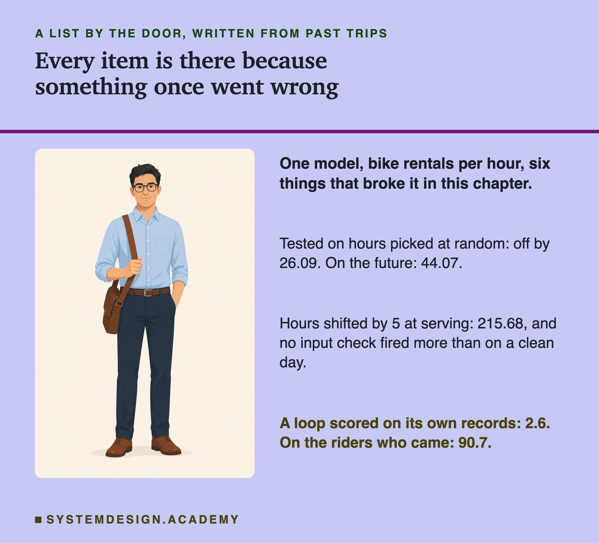
A list like that also has limits, and it helps to say them out loud. It only covers the trips he has already taken. It says nothing about a visa for a country he has never been to. A traveller who trusts the list completely will one day be caught by something that is not on it.

This lesson builds that kind of list for a program that learns from examples and is about to be used for real. Every line comes from something that went wrong earlier in this chapter, measured on real data. The last part of the lesson is about the list's limits: the things this chapter never tested.

This is the last lesson of the chapter. Over six lessons I took one program, which guesses how many bikes a city rents in an hour, and broke it in six different ways, one lesson at a time, always on the same public data: two years of hourly bike rentals from Washington, D.C.

Lesson 1 showed that the usual way of testing the program gave it a much kinder score than the future did. Lesson 2 let the world change under it: many more people rode in the second year. Lesson 3 computed one of its inputs a little differently at the moment it was used. Lesson 4 tested simple checks that could notice a broken input before the real answers came in. Lesson 5 asked whether watching how the inputs move could stand in for knowing how wrong the program is. Lesson 6 let the program's own decisions shape the data it learned from next.

Each lesson ended with advice. This lesson puts that advice in one place, in the order a team would actually use it, and next to each piece of advice it puts the number that earned it. Nothing new is measured here. Every number is read back from a file an earlier lesson stored, and checked again against the raw results of that lesson before it is shown.

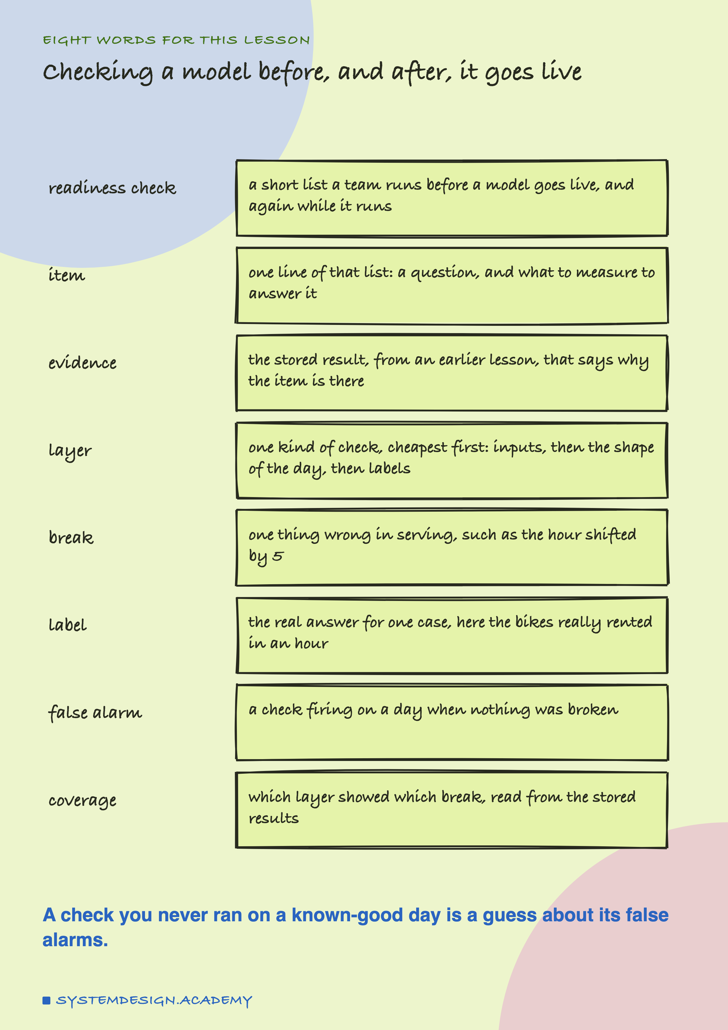
A model is a program that learned from examples to guess a number; here, the bikes rented in one hour. It is served when it is used for real, and the code that prepares its inputs at that moment is the serving code. A readiness check is a short list a team runs before a model goes live and keeps running while it is used. Each line is an item: a question, plus what to measure to answer it. The evidence for an item is the stored result, from an earlier lesson, that says why it is on the list.

A break is one thing that goes wrong at serving time, such as the hour of the day being sent 5 hours late. A layer is one kind of check that could notice a break, and the layers come in order of cost: checks on the inputs, then a check on the shape of a whole day, then the real answers. The real answer for one case is its label. A false alarm is a check firing when nothing was broken. Coverage, in this lesson, means which layer showed which break.

Two scores from the earlier lessons come back on almost every slide. The MAE (mean absolute error) is the average size of a miss, in rentals an hour. The signed error is the same average with the minus sign kept, so below zero means the guesses lean too low.

A checklist is only useful if it is in the order you meet the problems. Here is this chapter's list in that order.

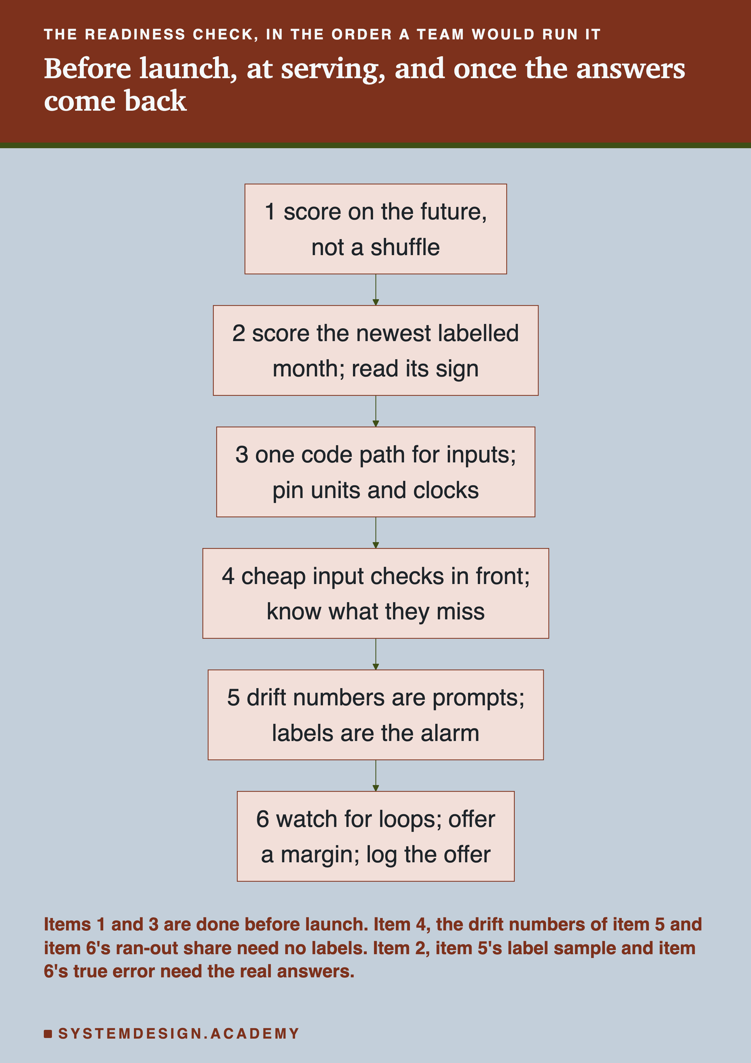
Item 1 comes before anything else, because it decides whether the number you ship with means anything: test the model on the future, not on a shuffle. Item 2 is the habit you keep once it is live: when a stretch of real answers arrives, score the model on it and read which way it leans. Item 3 is about the code that feeds the model: training and serving must compute each input the same way. It is a property of the code, settled before launch, not a check that runs every day. Item 4 puts cheap checks in front of the model, on every batch of inputs, before any answer can arrive. Item 5 is about the time between a guess and its real answer: numbers that describe how the inputs moved are a reason to look, not an alarm, and a small random sample of real answers is the better alarm. Item 6 asks whether the model's own decisions limit what can be written down, because then its records can hide its error.

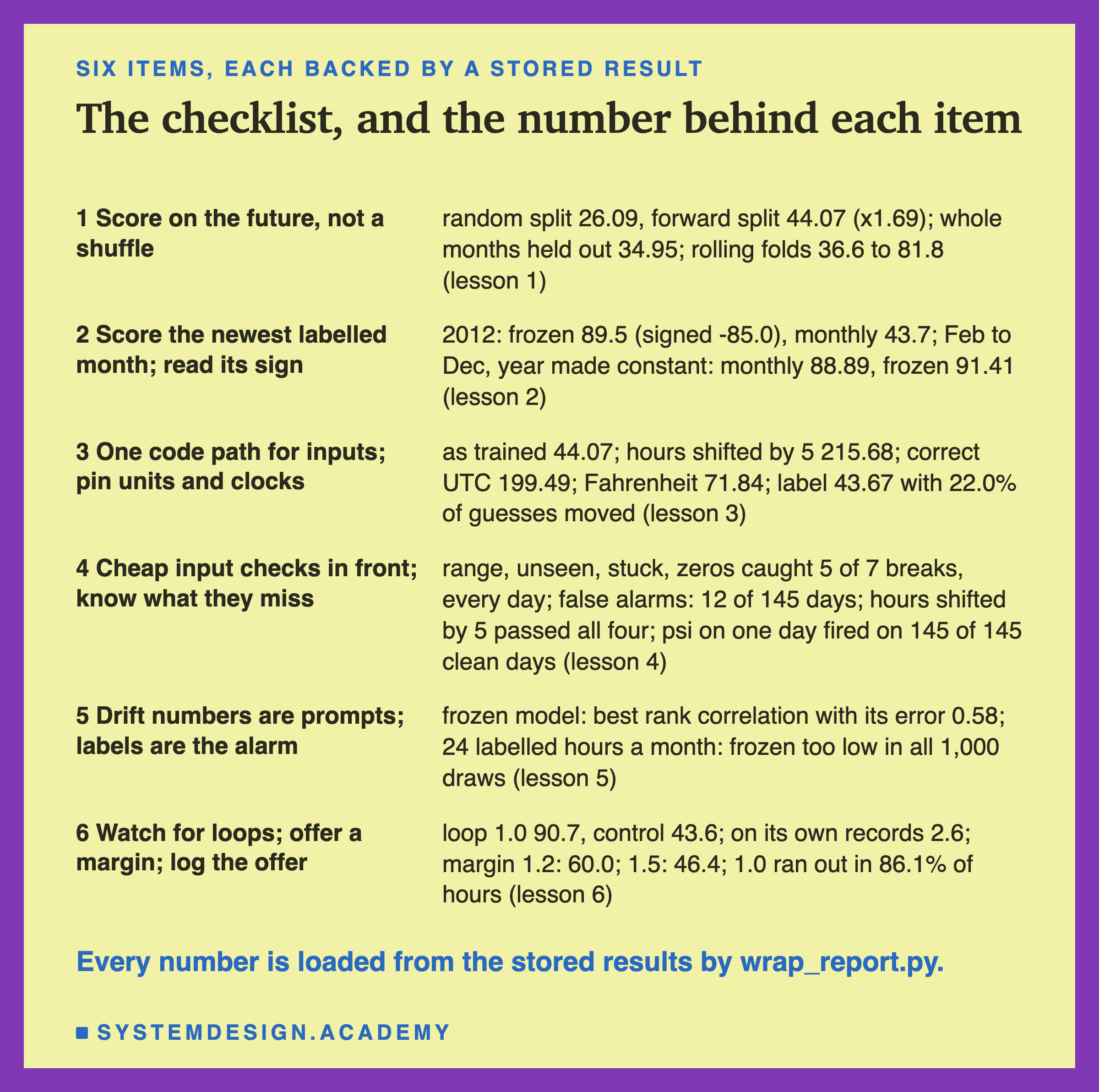
The list also says who does what. Item 1 belongs to whoever builds the model, and it is done before anyone else sees a number. Item 3 belongs to whoever writes the serving code, and it is easiest to do while that code is being written, not after. Items 2, 4 and 5 belong to whoever looks after the model once it is live: they are routines, run every batch or every month, and they only work if someone reads what they print. Item 6 belongs to whoever decides what the model's answer is used for, because only they know whether the answer limits what gets written down. A team that gives every item to one person usually finds that the items nobody owns are the ones that stop being run. That last point is my experience, not something this chapter measured.

This lesson trains no model and runs no model. I wrote one report for it, wrap_report.py, and it only reads files that the six earlier labs stored. For each item it reads that lesson's own result file, and where it can, it checks it against the raw rows the lesson kept.

Many of the checks are real recomputations, not a second copy of the same number; the rest compare a lab's own file with that lesson's report file. For lesson 1 the report computes the forward error again from all 3,476 stored guesses. For lesson 2 it computes the error over all 8,734 hours of 2012 from every stored guess, for each of the three policies (one of which never retrains). For lesson 3 it computes each condition's error and the share of guesses that moved from the stored guesses. For lesson 4 it compares every share in the table of checks with lesson 4's own report. For lesson 5 it computes all eight rank correlations again from the monthly numbers, with its own code. For lesson 6 it computes the loop's error on its own records, and the share of hours when every bike went, from the hour-by-hour file.

In all, the report makes 123 of these comparisons before it prints anything, and it stops if any one of them fails. They all agree.

It also follows every correction the lessons made after their reviews. The break that shifts every hour by 5 is called that, "hours shifted by 5", and not UTC, because lesson 3's follow-up found that a fixed +5 matches real UTC only for the last part of the test; with the correct offset the error was 199.49. Where a lesson's number came from a follow-up designed after its main results, this lesson says so too.

What came after all the results, and is mine alone: the order of the items, the wording of each item, which numbers stand for each one, and the coverage table later in the lesson. The report writes all of them from the stored files, but the choices behind them were made by reading the results.

The first question on the list is about the number you ship with. Lesson 1 found that the usual recipe, a random split, made the model look much better than it would ever be in use.

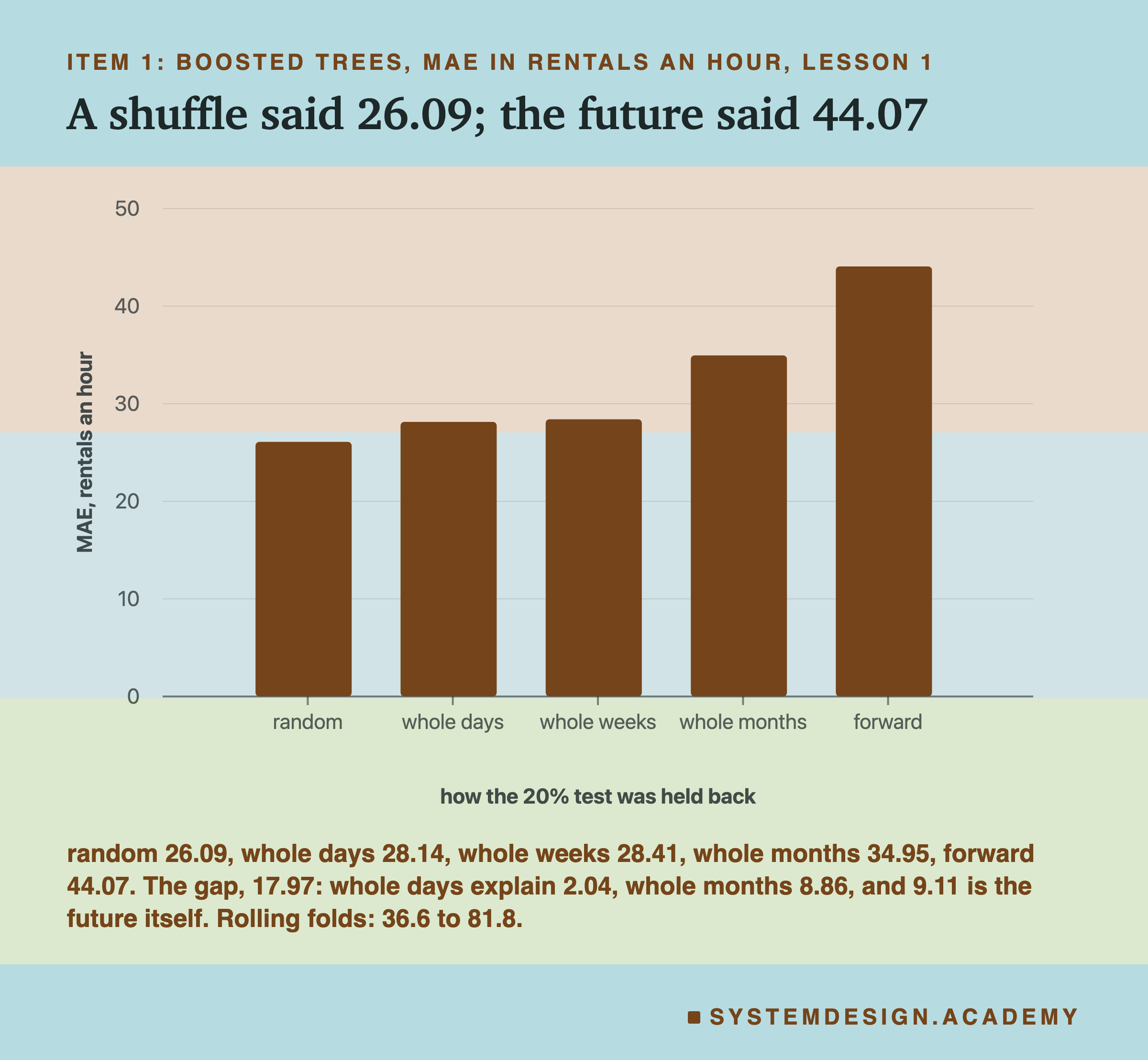
On hours picked at random, the boosted trees missed by 26.09 rentals an hour. That is the mean of five random splits, each shuffled from a different seed (a starting number for the shuffle, so the same seed always gives the same split); the five ran from 25.60 to 26.74. On the last 20% of the hours in time, the future the model would really meet, they missed by 44.07: 1.69 times as much, a gap of 17.97.

A follow-up in lesson 1, designed after the main results and prompted by a review, measured where that gap came from. It held back whole days, weeks or months at random instead of single hours. Whole days gave 28.14, only 2.04 of the 17.97 points: the neighbouring hours in training explain little. Whole weeks gave 28.41. Whole months gave 34.95, 8.86 points, about half the gap: the random test had seen other hours of each test month while it learned. The last 9.11 points, from 34.95 to 44.07, went with the future itself, which was also busier than the past.

The forward score also depends on which stretch of the future you test. Five rolling folds, each trained on everything before its own block, scored between 36.6 and 81.8.

So the item is: hold the test back by time, roll it forward a few times, and report the spread. The question to ask of your own model: was the test held back by time, the way the model will really be used? In lesson 1's code the change was one line, slicing the rows in time order instead of shuffling them. If the rows have a time and the model will only meet later rows, a random split describes a job the model will never do.

Once the model is live, the next item is a habit. Lesson 2 trained the model on 2011 and used it through all of 2012, while the city's riders grew a lot.

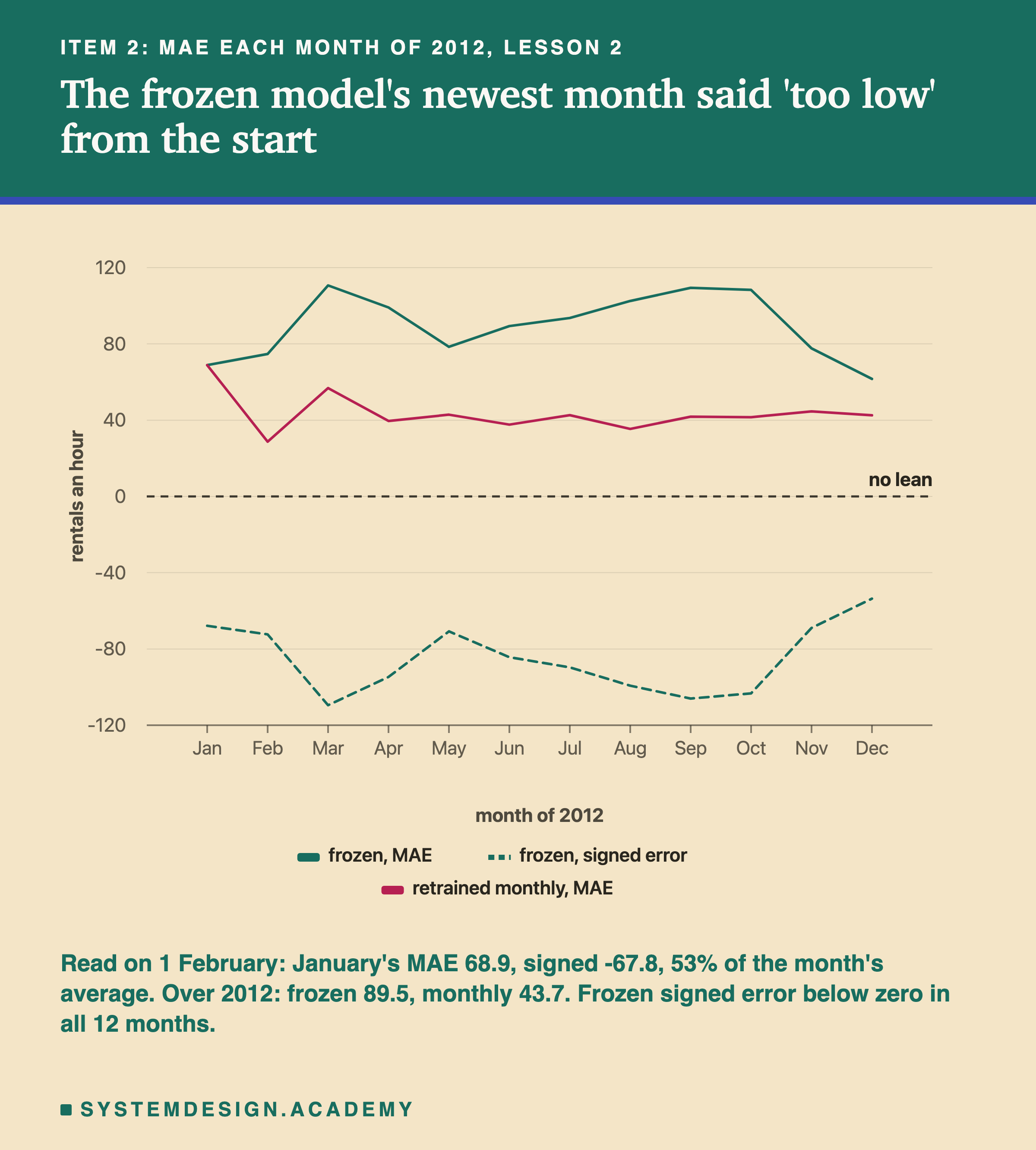
Lesson 2 compared three policies, rules for when to retrain. The model that was never retrained, the frozen one, missed 2012 by 89.5 rentals an hour, with a signed error of -85.0: almost all of its error was guessing too low, on 85.5% of the hours. Retrained every month on everything so far, the model missed by 43.7. Retrained every month on only the last 12 months, a window, it missed by 47.9. And the frozen model's problem was visible on the first day it could be: on 1 February, January's real counts gave an MAE of 68.9, which was 53% of the month's average, and a signed error of -67.8, so the misses were almost all too low.

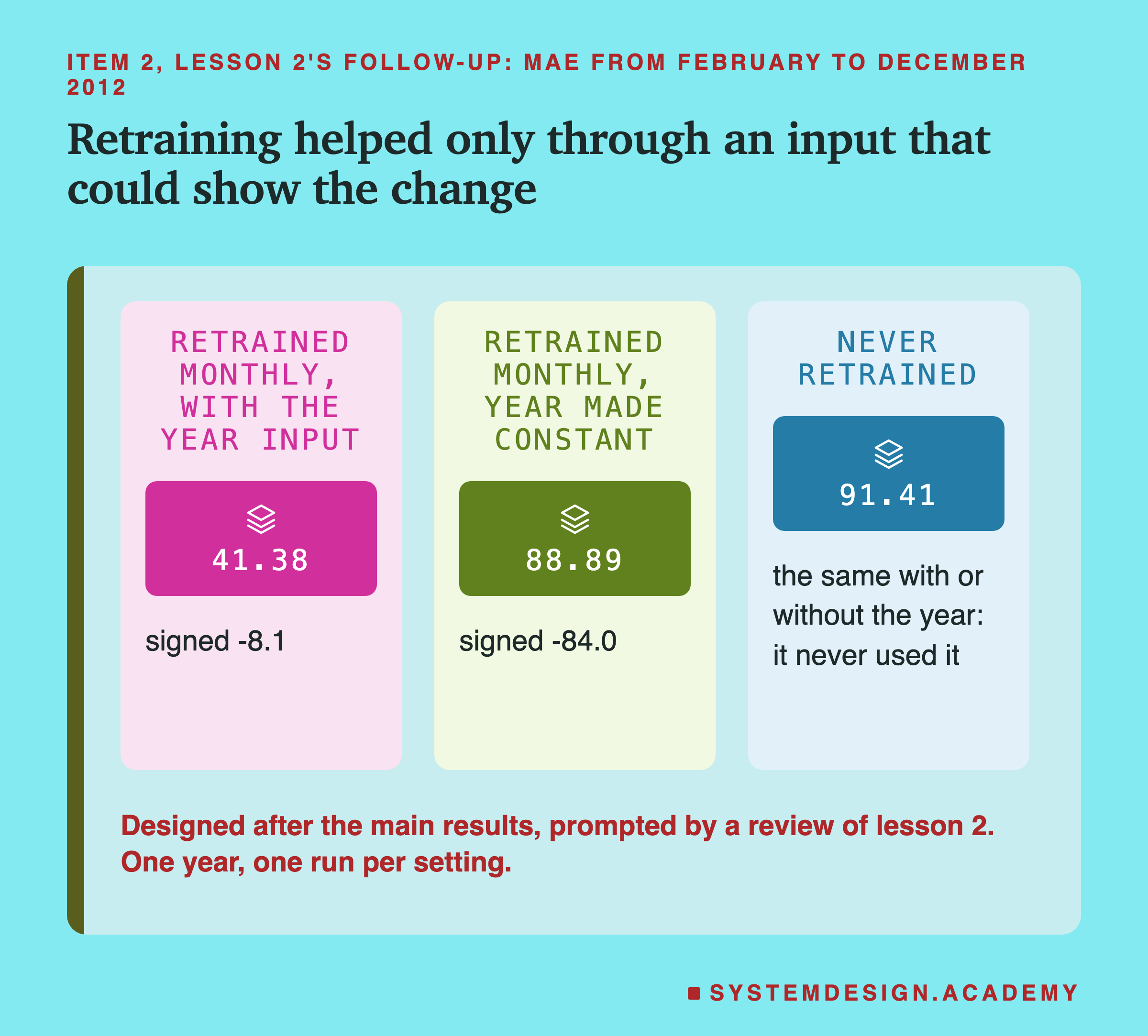
The follow-up is the part of this item people skip. Lesson 2's review asked why retraining helped, and a follow-up, designed after the main results, made the year column constant so that no tree could use it. From February to December, retraining monthly then scored 88.89, against 91.41 for the frozen model, and it kept the lean (signed -84.0). With the year input it had scored 41.38. So retraining caught up here only because one input could say "this row is from the new, busier year".

The third item is about the code that feeds the model. Lesson 3 kept the model and the test hours fixed and changed only how one input was computed at serving time, one input at a time.

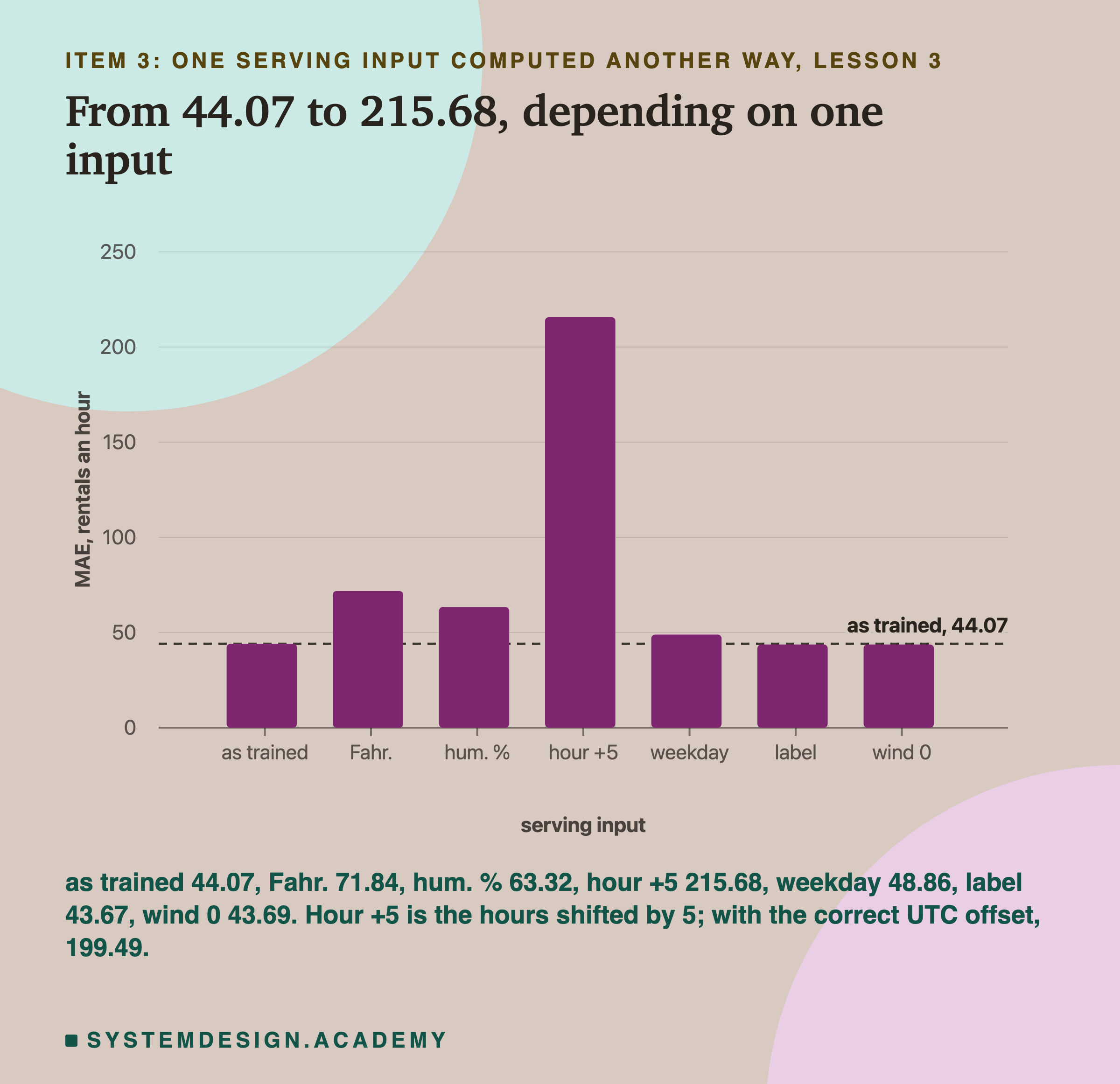
With the inputs computed as in training, the model missed by 44.07. With every hour shifted by 5, it missed by 215.68, almost five times as much. UTC is the world's reference time; Washington was 4 hours behind it until 4 November 2012 and 5 hours after, and with that correct offset the error was 199.49. Temperatures sent in Fahrenheit gave 71.84, and it was the only break that produced impossible answers: 54 guesses below zero bikes. Humidity sent as a percentage gave 63.32 and pushed the guesses much lower (signed -42.5). The weekday counted from Monday instead of Sunday gave 48.86. In none of these cases did the model complain. It answered every time.

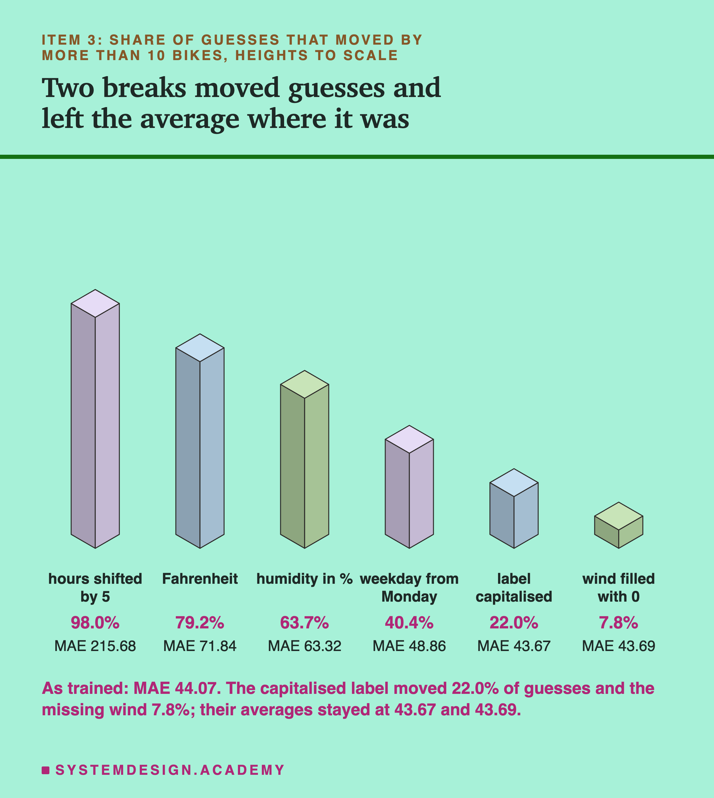
Two of the six breaks are the reason this item also says the average error cannot be the alarm. A weather label spelled with a capital letter moved 22.0% of the guesses by more than 10 bikes, and a missing wind speed filled with 0 moved 7.8%, yet their average errors were 43.67 and 43.69, next to the 44.07 as trained. Lesson 3 found why for the label: every hour was treated as clear, rainy hours got worse and misty hours better, and the two nearly cancelled.

The item: compute each input with one shared function, used in training and in serving; write every unit, time zone and allowed word into a schema, a written description of each input; and never judge a serving change by the average error alone. Lesson 3 measured the damage only. It did not test any fix, so this half of the item is common practice, not something these numbers prove.

The fourth item is about the time before the real answers arrive. Lesson 4 served the model 145 test days, broke one input at a time in seven ways (lesson 3's six plus a stuck temperature sensor), and ran six simple checks on every day.

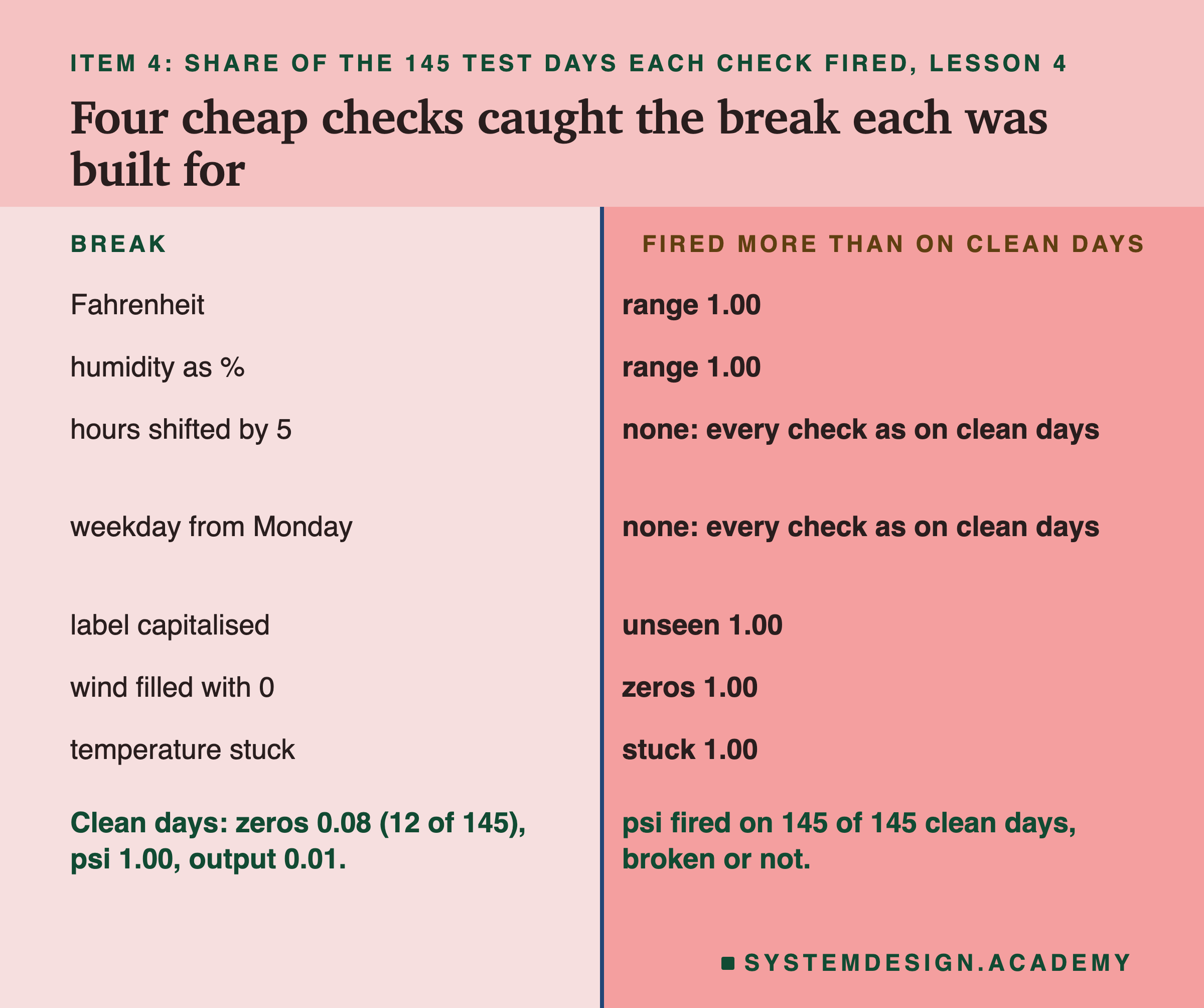
Four cheap checks each caught the break they were built for, on every day: the range check (a number outside what training ever had) caught Fahrenheit and humidity as a percentage; the unseen check (a word training never had) caught the capitalised label; the stuck check caught the stuck temperature; and the zeros check caught the wind filled with 0. Together they caught 5 of the 7 breaks, and their only false alarms were 12 calm days out of 145 for the zeros check. The worst break, the hours shifted by 5, and the weekday counted from Monday got past all four: their values stayed inside the normal range, so no check that looks at one column at a time could see them.

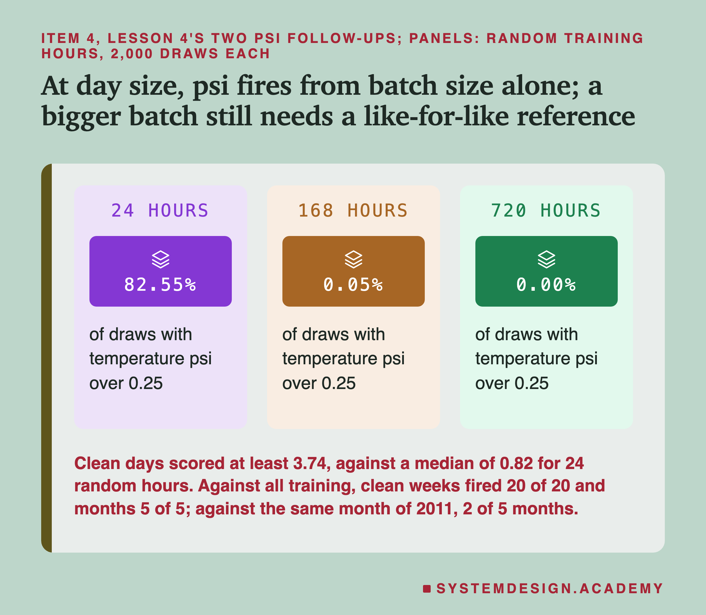
The fifth check failed in a way worth remembering. The psi (population stability index: one number for how far the mix of values in a column moved), with its usual line of 0.25, fired on all 145 clean days. Lesson 4 ran two follow-ups, both designed after the main results. The first made the batches bigger and changed the reference. Against all the training hours, clean weeks still fired on 20 of 20 and clean months on 5 of 5. Against the same month of 2011, clean months fired on 2 of 5, because the weather really did differ from a year before.

The fifth item is about what to watch while the real answers are late. Lesson 5 computed four measures of how the inputs and outputs moved, month by month through 2012, and ranked each against the model's real error.

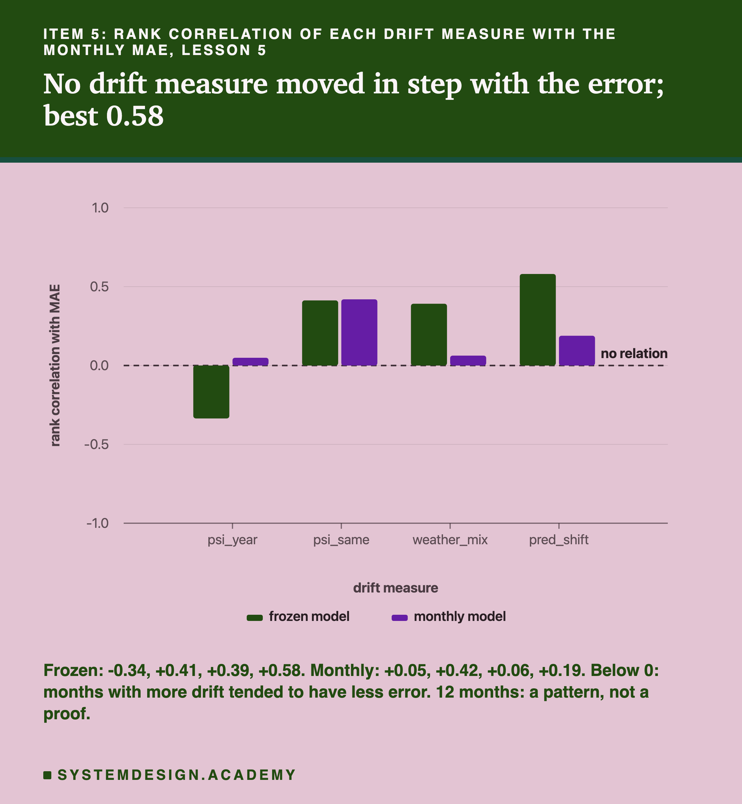
A rank correlation (the kind called Spearman's) says whether two lists rise and fall in the same order: 1 is the same order, 0 no same-order relation, and a value below 0 means they tend to move in opposite orders. The best of the four measures, for the frozen model, reached 0.58. The usual psi, against the whole training year, reached -0.34: its months with more drift tended to be months with less error. None moved in step with the error. Lesson 5 found why: over the year, the weather of 2012 looked much like 2011's, while the riders grew by 1.41 to 2.53 times, month by month. The error came from the riders, which no weather input carries.

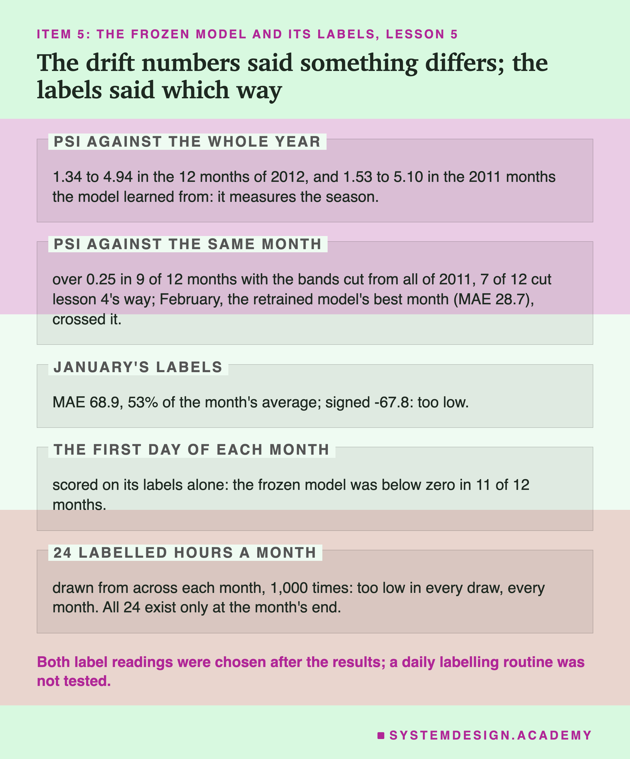
The drift numbers were also noisy as alarms. The whole-year psi sat between 1.34 and 4.94 every month of 2012, and between 1.53 and 5.10 in the 2011 months the model had learned from: it was measuring the season. The same-month psi crossed 0.25 in 9 of 12 months, including February, which was the retrained model's best month of the year. And that count depends on how the bands are cut: cut from each month of 2011 itself, the way lesson 4 did, it crossed the line in 7 of 12 months instead of 9. A line whose verdict moves with a choice like that is a weak alarm.

The last item is about a model whose answer changes what can happen next. Lesson 6 was a simulation: the hourly counts were real and played the demand, but the rule that placed bikes from the forecast was invented. Riders could only rent bikes that were there, and each month's model learned from what was rented.

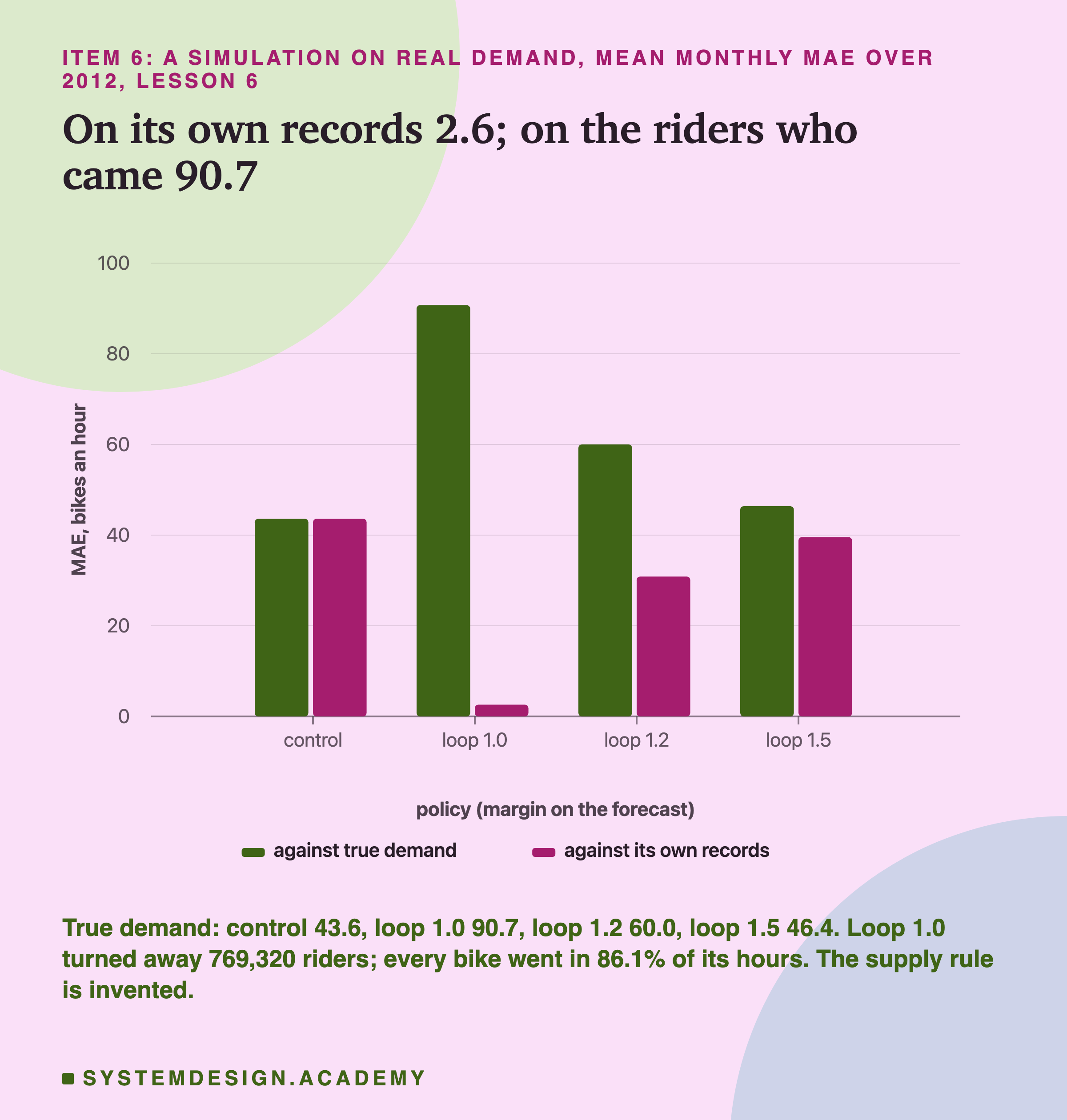
With no margin (loop 1.0), the model missed the riders who really came by 90.7 bikes an hour, against 43.6 for a control that learned from every rider, and it turned away 769,320 riders over the year. Scored on its own records, the only error an operator could compute, it missed by 2.6. Every record was true; the riders who found an empty rack were never written down. Bikes placed at 20% above the forecast brought the error to 60.0, and at 50% to 46.4, at a cost of 820,304 idle bike-hours. That last number is a unit of this simulation, which counts a bike again every hour it stands unused.

One number was visible to the operator at once, with no labels and no knowledge of demand, and it pointed straight at the problem: in 86.1% of loop 1.0's hours, every bike placed was rented. Only the error against true demand needed the real counts.

The item: ask whether the model's answer limits what can be recorded; if it does, log what was offered as well as what was taken, count how often the offer ran out, keep a margin, and never judge the model only on its own records. Lesson 6 tested margins only. Making a small share of decisions without the model is common advice with the same aim, and it was not tested here. The same shape appears in recommendations, fraud rules, credit and stock ordering, but those were general knowledge in lesson 6, not measured.

A list is easier to use when you know where each line happens. This sequence places the items in one day of a model in service.

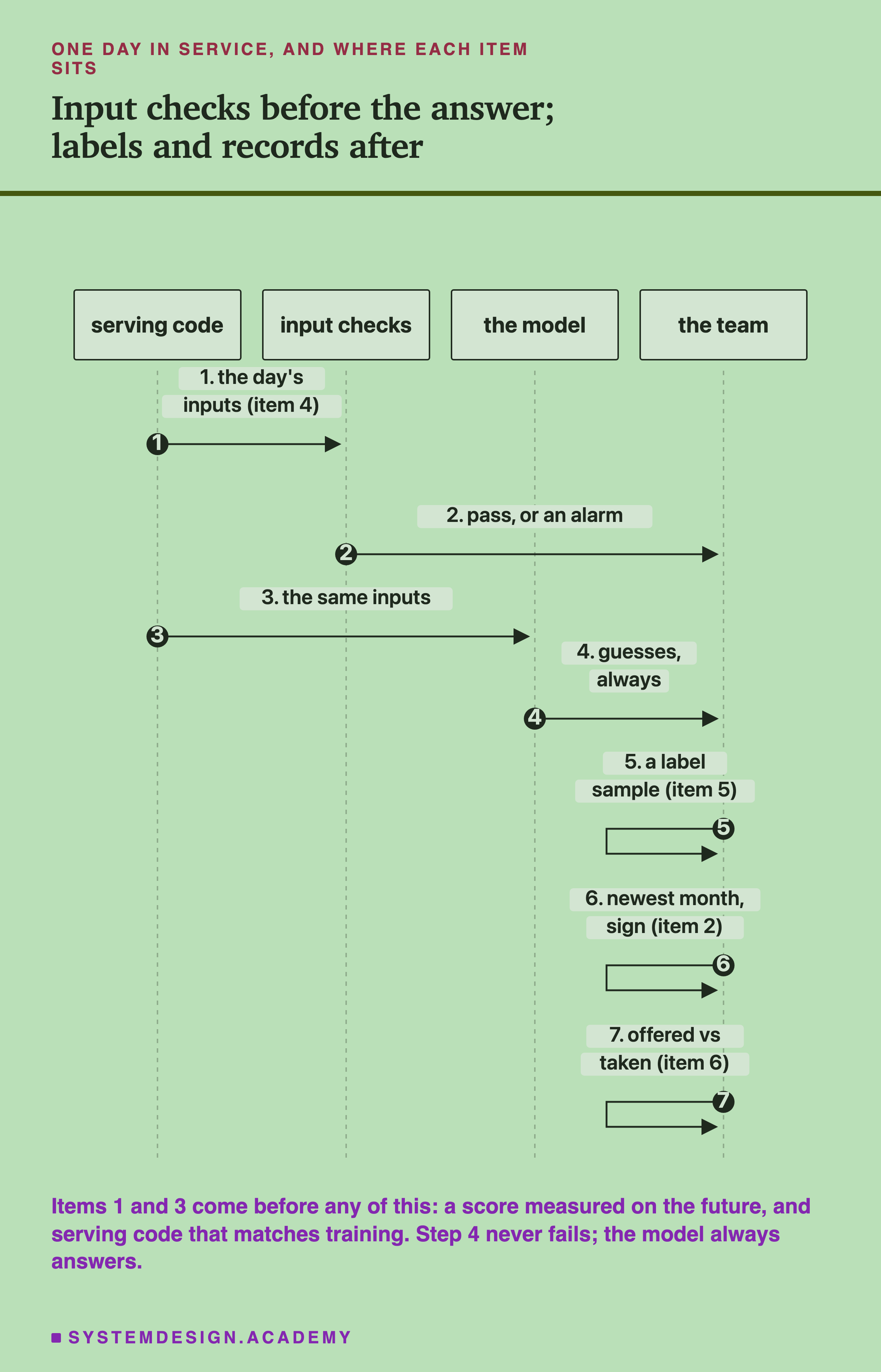
The serving code builds the inputs, and the cheap checks read them before anything else happens. The model always answers, broken input or not; that was the point of lesson 4's title. Then the team's work begins: a sample of labels as they can be had, the newest labelled month when it is complete, and, for a model that decides something, a record of what was offered next to what was taken. Items 1 and 3 do not appear in the day at all, because they are settled before launch.

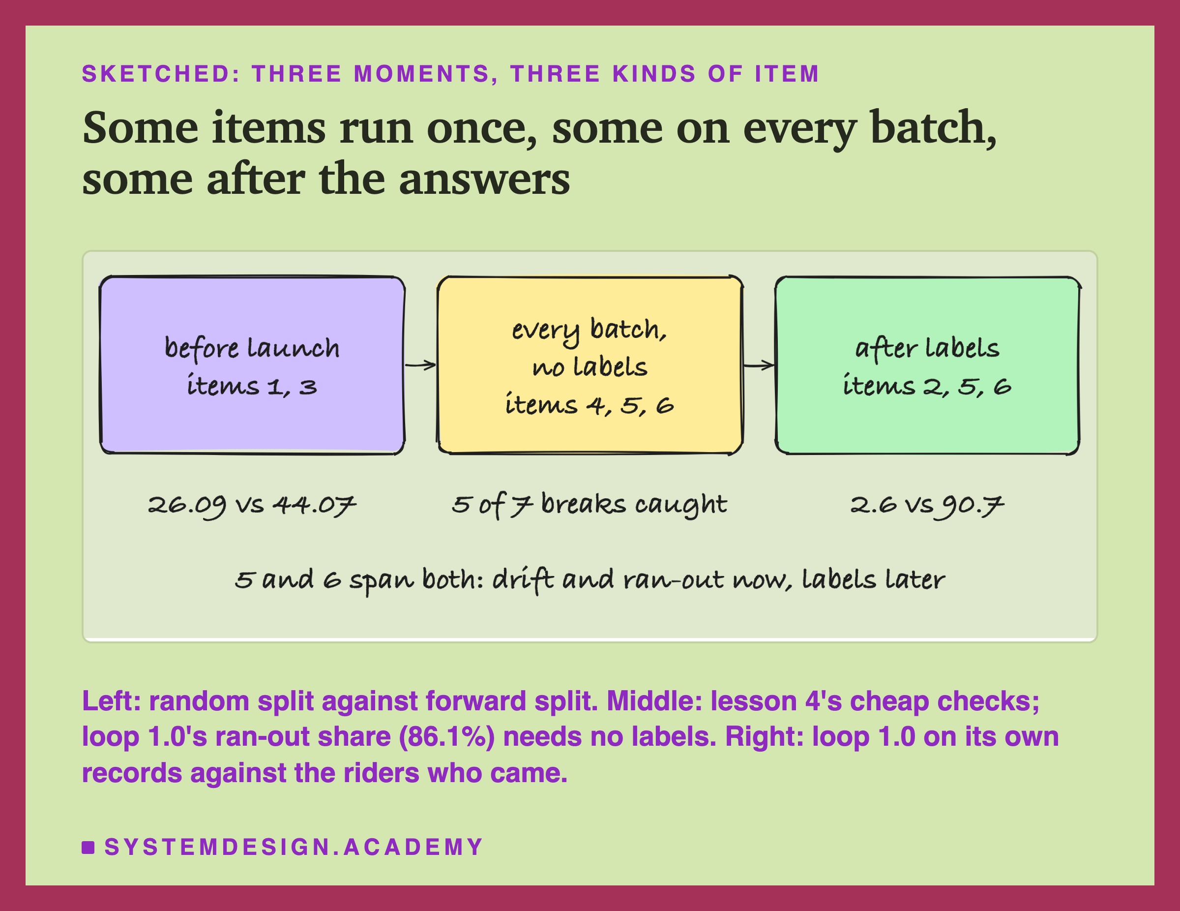
The sketch groups the same items by when they run. Items 1 and 3 run once, before launch, and again whenever the model or its serving code is rebuilt. Item 4 runs on every batch, before any label exists, which is why its checks have to be cheap and why their false alarms matter so much. Items 5 and 6 sit on both sides. Drift numbers and the share of hours when every bike went can be read at once, with no labels. The label sample of item 5 and the true-demand error of item 6 need the real answers, and so does item 2. A team that only has the items on the right finds out about a break when the damage is already done; a team that only has the checks in the middle sees many breaks early and misses the ones that stay in range.

After all the results were in, I put lesson 4's breaks next to each layer that could have shown them. This table is derived from the stored files; nothing in it was measured for this lesson.

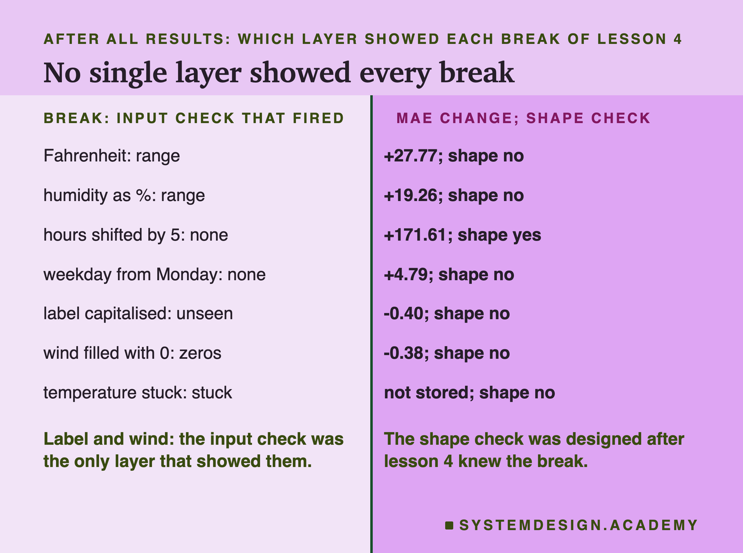
Read it row by row. The unit breaks were caught by the range check and also raised the real error, by 27.77 and 19.26 rentals an hour: two layers saw them. The hours shifted by 5 passed every input check, raised the real error by 171.61, and only the shape check, built after the fact, saw it before the answers came. The weekday counted from Monday passed every check, including the shape check, and showed up only in the real error, as a rise of 4.79. The capitalised label and the missing wind speed were the opposite: the real error did not rise at all (it moved by -0.40 and -0.38), and only the input checks saw them. The stuck temperature was caught by its check, and its cost is unknown, because lesson 4 did not store its guesses.

So the answer to "which layer should we build?" is: more than one. Here, the input checks alone would have missed the most costly break, the hours shifted by 5, and the weekday break; the real error alone would have missed the two that moved hundreds of guesses (22.0% and 7.8% of 3,476) without moving the average. That is my reading of seven rows from one run, not a law. What it does show is that each layer saw something the others could not.

A checklist built from six lessons is only as wide as those lessons. Here is what they covered, and what they did not.

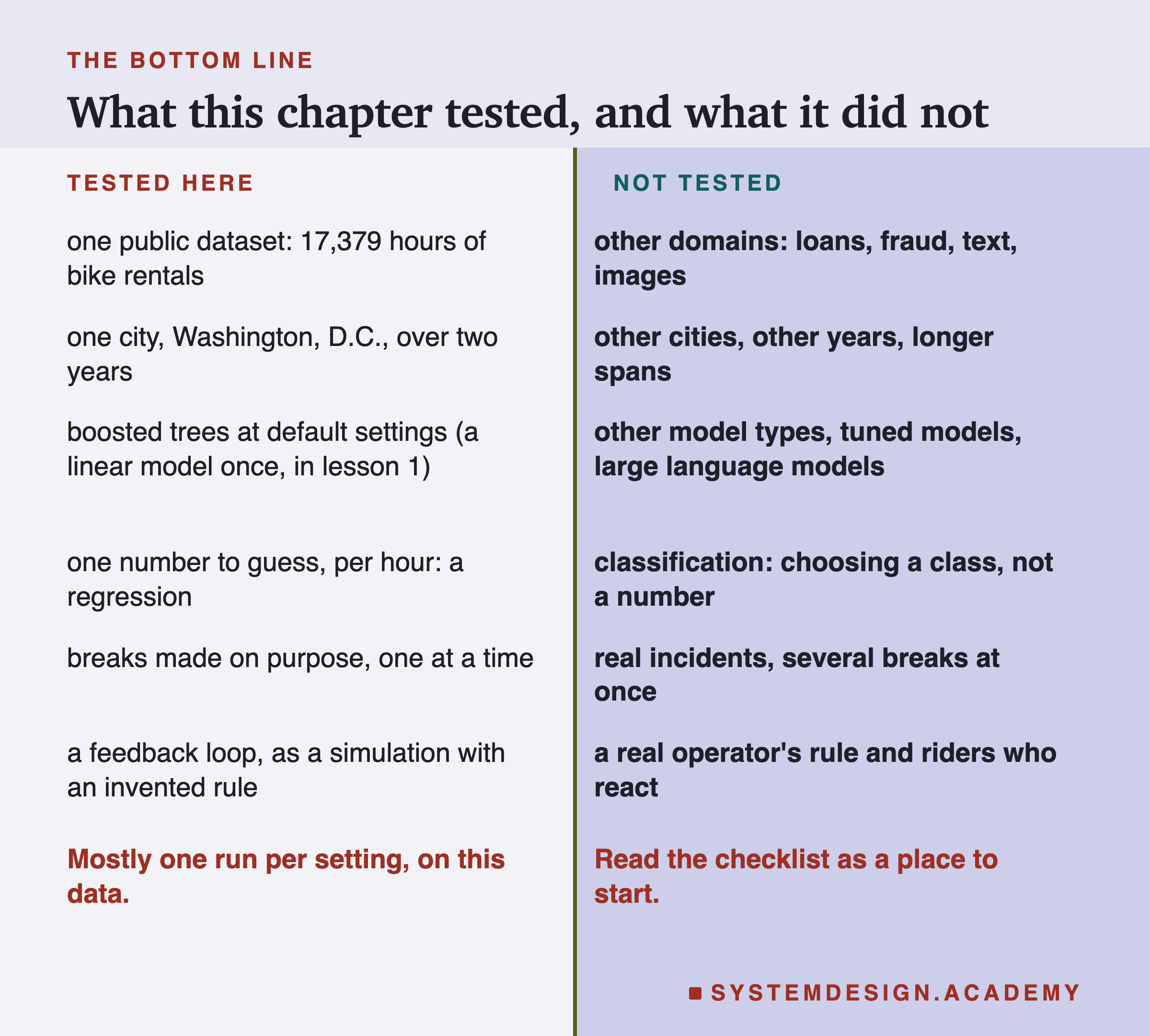
One dataset, one city, two years. Every number in this chapter comes from 17,379 hours of bike rentals in Washington, D.C., in 2011 and 2012. The kind of drift here was mostly one kind: many more riders, with weather much like the year before. Data where the inputs themselves change a lot, or where the world turns around rather than growing, could rank these items differently.

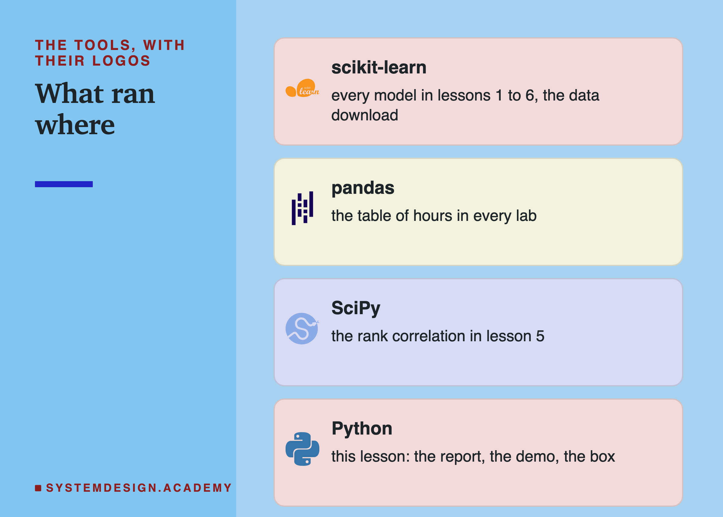
One model family. Every lesson used scikit-learn's boosted trees at default settings; lesson 1 added a linear model once, as a check. Some findings depend on how trees work. A tree cannot extend what it learned past the range it saw, which is why Fahrenheit acted like the hottest training hour. A linear model would react differently, and a large language model very differently. None was tested here.

Regression only. The model guessed a number. Nothing in this chapter tested classification, where a model chooses a class (fraud or not, spam or not). Its errors are counted differently, and some items, such as reading the sign of the error, change shape there.

Breaks made on purpose, and a simulated loop. Every break was applied by me, one at a time, to every hour. Real incidents start in the middle of a day, affect some requests and not others, and arrive several at once. The loop was a simulation with an invented rule, and its riders never reacted to an empty rack.

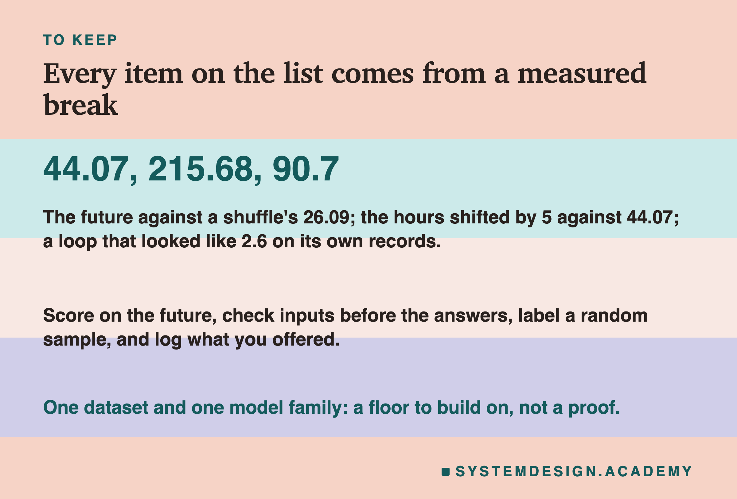
Mostly one run per setting. Each lab ran its design once. Only lesson 1's random split used five seeds; lesson 2's follow-up cut the monthly policy's rows with three seeds, and lesson 5 drew its label samples 1,000 times. The designs were written before the runs, and every follow-up was designed after its lesson's results. So the checklist is a floor to build on: each item is here because something broke on this data. What it cannot tell you is what will break on yours.

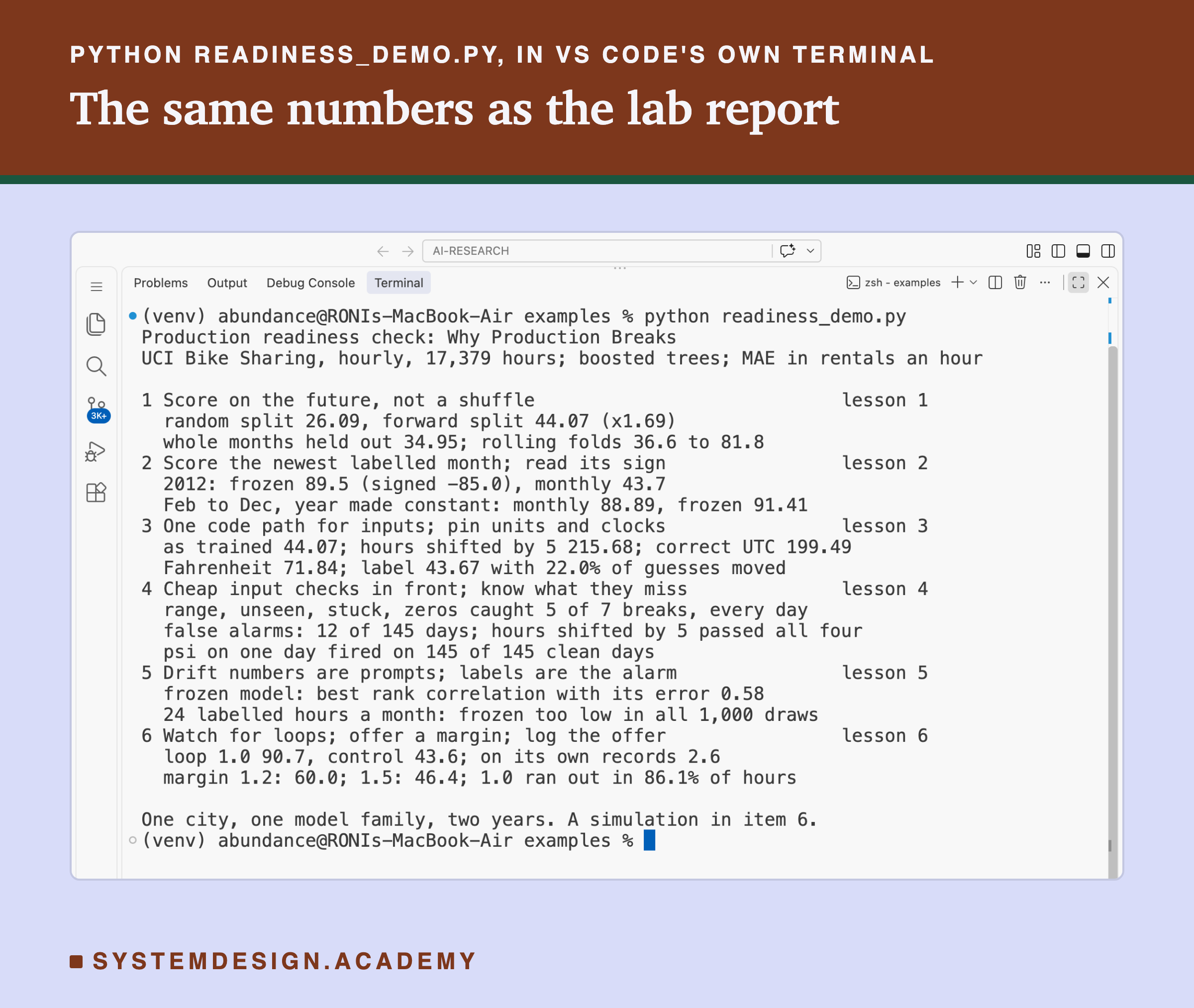
This script prints the checklist with each item's measured evidence, or one item with the question to ask of your own model. It uses only Python's standard library, reads one small file, and runs no model.

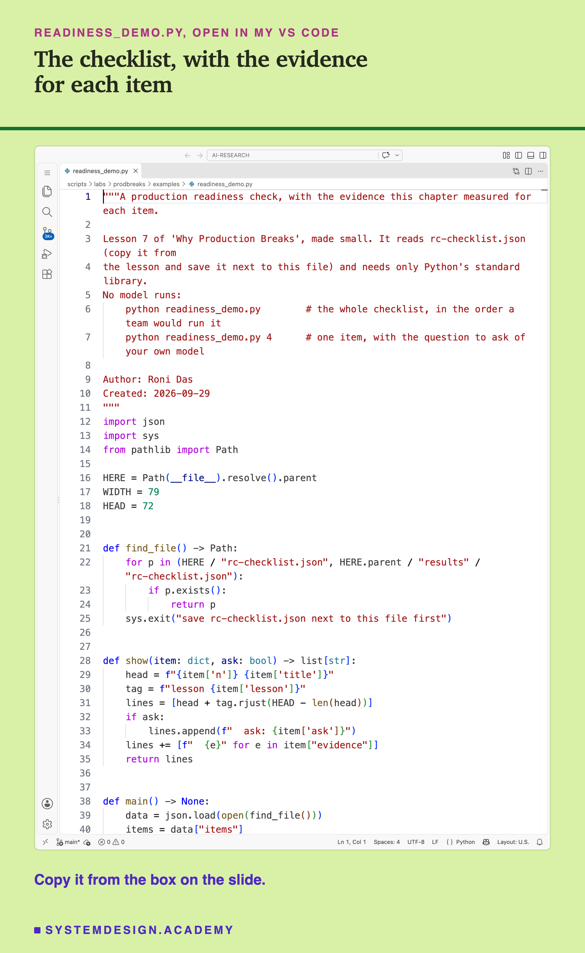
Before you run this lab. This script needs only Python 3; it installs nothing and calls no model. It reads rc-checklist.json, printed in full in the second box below: save it next to the script. The chapter's own labs used scikit-learn and pandas (pip install scikit-learn pandas), and each earlier lesson says how to run them.

"""A production readiness check, with the evidence this chapter measured for each item.

Lesson 7 of 'Why Production Breaks', made small. It reads rc-checklist.json (copy it from
the lesson and save it next to this file) and needs only Python's standard library.
No model runs:
    python readiness_demo.py        # the whole checklist, in the order a team would run it
    python readiness_demo.py 4      # one item, with the question to ask of your own model

Author: Roni Das
Created: 2026-09-29
"""
import json
import sys
from pathlib import Path

HERE = Path(__file__).resolve().parent
WIDTH = 79
HEAD = 72


def find_file() -> Path:
    for p in (HERE / "rc-checklist.json", HERE.parent / "results" / "rc-checklist.json"):
        if p.exists():
            return p
    sys.exit("save rc-checklist.json next to this file first")


def show(item: dict, ask: bool) -> list[str]:
    head = f"{item['n']} {item['title']}"
    tag = f"lesson {item['lesson']}"
    lines = [head + tag.rjust(HEAD - len(head))]
    if ask:
        lines.append(f"  ask: {item['ask']}")
    lines += [f"  {e}" for e in item["evidence"]]
    return lines


def main() -> None:
    data = json.load(open(find_file()))
    items = data["items"]
    pick = sys.argv[1:2]
    if pick:
        n = int(pick[0])
        if not 1 <= n <= len(items):
            sys.exit(f"choose an item from 1 to {len(items)}")
        items = [items[n - 1]]
    out = [data["title"], data["scope"], ""]
    for item in items:
        out += show(item, ask=bool(pick))
    out += ["", data["footer"]]
    too_long = [line for line in out if len(line) >= WIDTH + 1]
    if too_long:
        sys.exit(f"a line is longer than {WIDTH} characters: {too_long[0]}")
    print("\n".join(out))


if __name__ == "__main__":
    main()

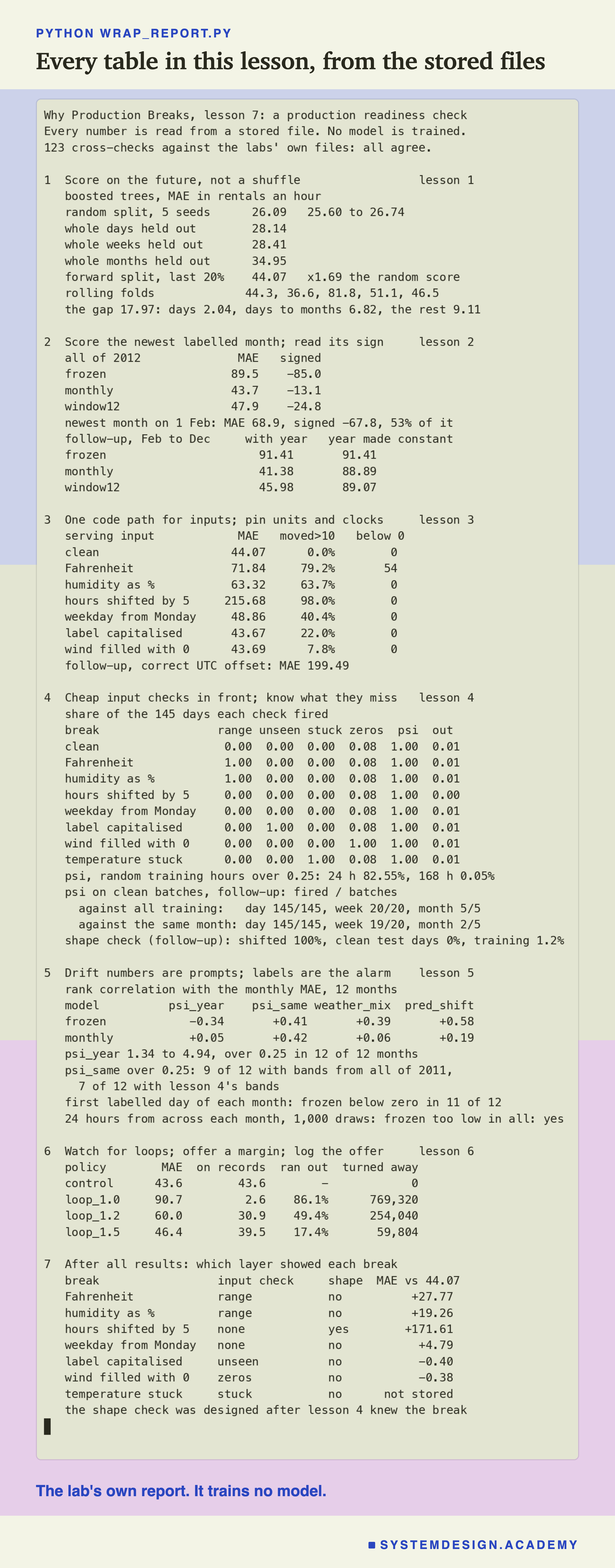
The report lives in scripts/labs/prodbreaks/wrap_report.py. It reads each lesson's lab files from scripts/labs/prodbreaks/results/: split.json and split_blocked.json for lesson 1, drift.json and drift_followup.json for lesson 2, skew.json and skew_followup.json for lesson 3, checks.json, checks_followup.json and checks_psi_size.json for lesson 4, watch.json for lesson 5, and loop.json and loop_detail.json for lesson 6. It checks each one against that lesson's own report file ( to ), recomputing from the stored guesses and hourly rows wherever the lab kept them. If any of the 123 comparisons fails, it stops before printing.

This box has no model in it. It holds the six items with their evidence, lesson 4's table of how often each check fired under each break, lesson 3's error and moved share for each serving input, and the coverage table. It runs in your browser.

As it is, the box prints the checklist with its evidence, then the coverage table: for each of lesson 4's breaks, which input check fired, whether the shape check fired, and the change in the error from 44.07 (for example +171.61 for the hours shifted by 5 and -0.40 for the capitalised label). The report's box mode checks every printed evidence line and every coverage row against its own numbers.

Try item(4) to see one item with the question to ask of your own model. Try caught('weekday_shift') to confirm that no check fired more often than on clean days, and caught('wind_missing') to see the zeros check. Then describe your own set-up: gaps(forward_test=True, same_code=True) lists the items you did not name, each with what this chapter measured for it. The names it knows are forward_test, newest_month, same_code, input_checks, early_labels and loop_log.

Finding the file. find_file looks for rc-checklist.json next to the script, and if it is not there, in the lab's results folder. If neither exists, it stops with a message rather than guessing.

One item. show builds the lines for one item: its number and title, with the lesson it came from lined up on the right at column 72, then its evidence lines, indented by two spaces. When you ask for one item, it also prints the question to ask of your own model.

The whole list. main reads the file, keeps either all six items or the one you named on the command line, and adds the title, the scope and the closing line. Before it prints, it checks that no line is 80 characters or longer, so the output fits an ordinary terminal without wrapping; if one were, it would stop and say which.

Where the numbers come from. Nothing in the script computes a result. The evidence lines are written by wrap_report.py, which builds each one from the stored results after its 123 checks, so the demo can only print what the labs measured. In the report, each item has its own function (item1 to item6) that loads one lesson's files, recomputes what it can, and returns the numbers; checklist turns them into the six items, using one list of titles that the report's own headings use too, and coverage builds the table of which layer showed which break.

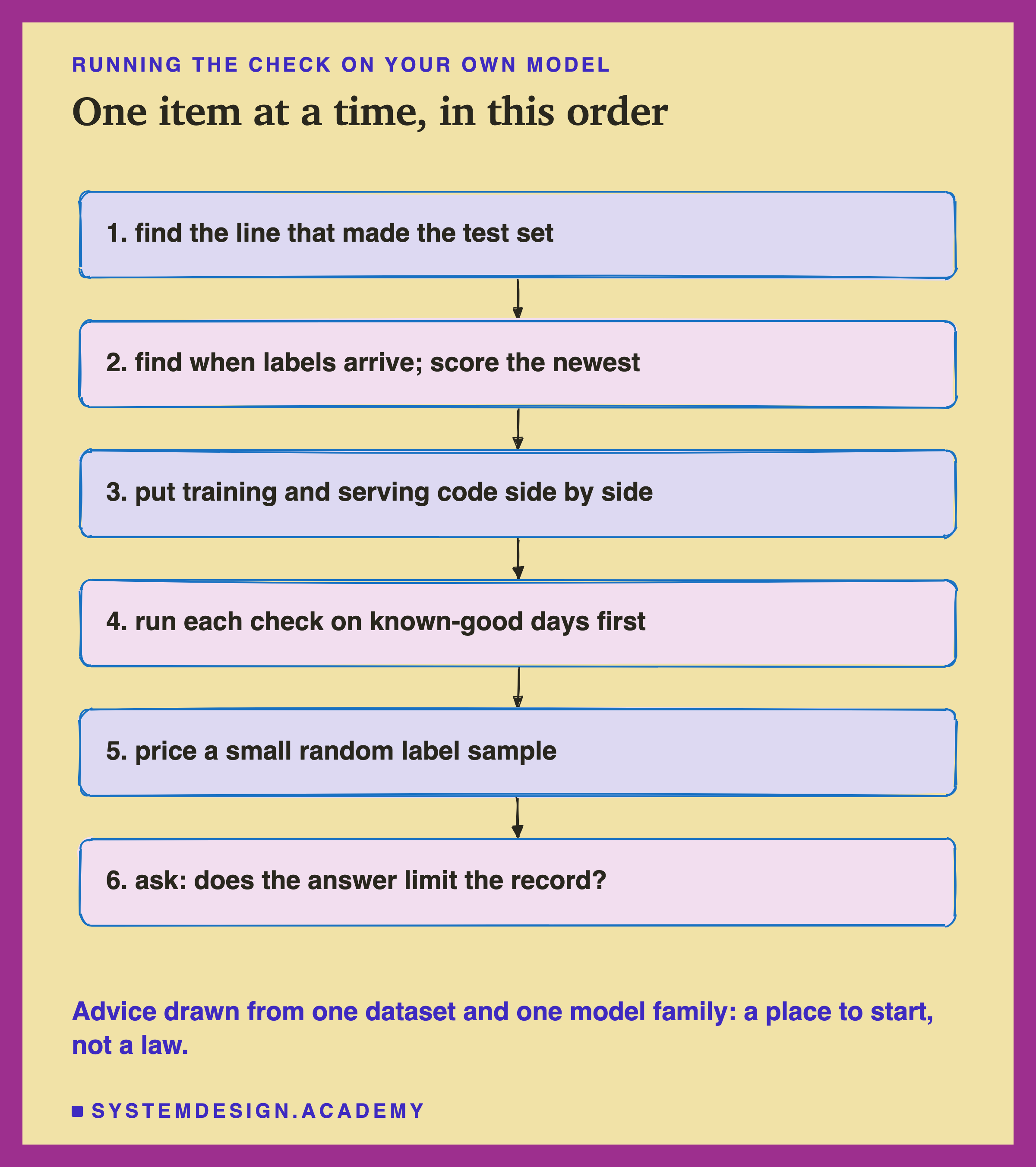
Find the line that made the test set. If the rows have a time and it shuffles them, change it to a cut in time, run the score again, and roll it forward over a few later stretches. Write down the spread. That is the number you ship with.

Find out when the real answers arrive, and score the newest stretch. Write down the MAE, the signed error and the MAE as a share of the average, next to the launch numbers. Then ask what input could show the change you most expect.

Put the training code and the serving code side by side. Run the training code on a hundred real serving records and compare the inputs value by value. Look hardest at time stamps, units, day numbering, words and missing values.

Run every check on days you know were fine before anyone gets an alarm. Range, unseen words, stuck values and counts of zeros are a few lines each. Count how often each fires on clean data; a check that fires every day gets ignored.

Price a small random sample of labels. Find out what one label costs, and how many a month you can afford. Here 24 a month showed the frozen model's lean in every draw, and the first day alone showed it in 11 of 12 months.

Ask whether the model's answer limits what gets recorded. If it does, start logging what was offered, not only what was taken.

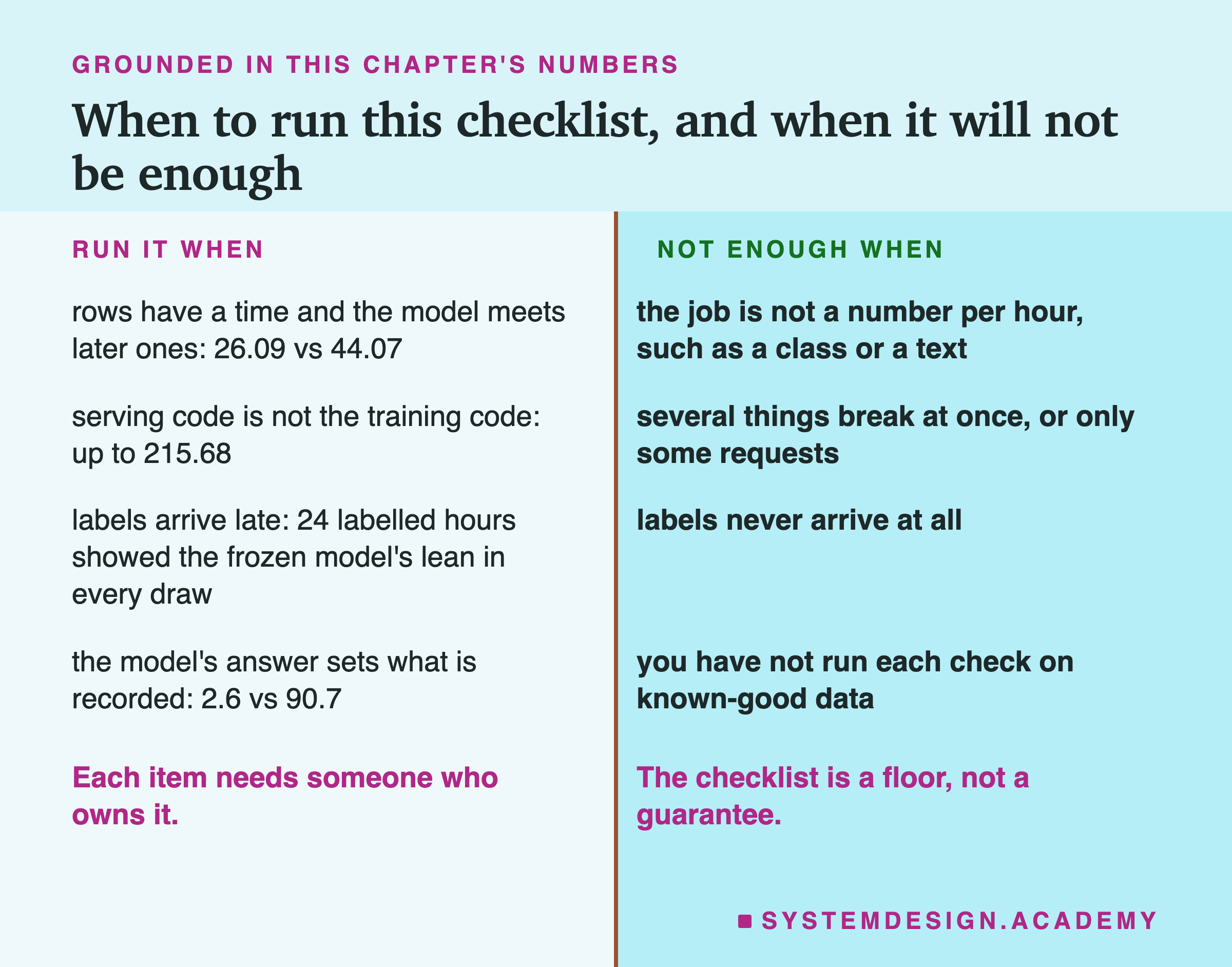
Use it when your model guesses a number from rows that arrive in time. Demand, traffic, prices, sensor readings. That is the kind of job this chapter measured, and every item has a number from it: a shuffle said 26.09 where the future said 44.07.

Use it when serving code is written separately from training code. A different team, a different language, a data provider. One line in that code moved the error to 215.68 here.

Use it when labels arrive late. Items 4 and 5 are about that gap: cheap checks on every batch, drift numbers read as prompts, and a small random sample of labels as soon as you can afford one.

Use it when the model's answer decides something. Stock, supply, a ranked list, an approval. Item 6 is the one that stops a model being judged on records its own decisions shaped.

Do not treat it as enough when the job is different. Classification, text, images or ranking were not tested here; the items still make sense, but the numbers behind them do not transfer, and each needs its own measure of error.

Do not treat it as enough when things break in messier ways. Several breaks at once, a break in only some requests, or labels that never arrive at all were not tested. And a check you have never run on known-good data is not yet a check: you do not know its false alarms.

Do not use it as a score. Passing all six items does not mean a model is safe. It means it does not fail in the six ways this chapter found.

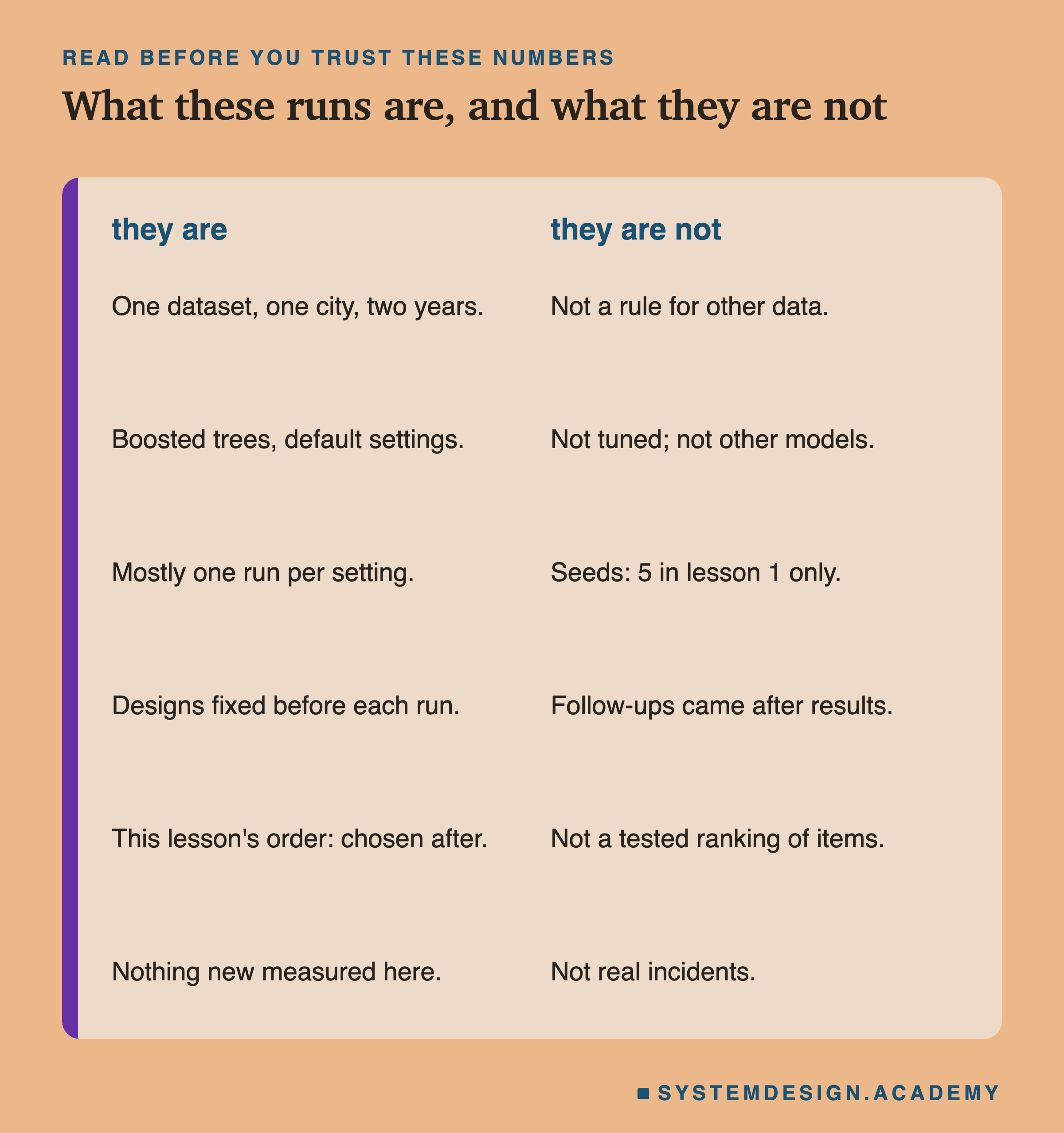
Nothing new was measured. Every number in this lesson was stored by an earlier lesson and read back here, after 123 checks against the labs' own files. So every limit of those lessons applies here too, and I repeat the main ones.

One dataset, one model family, mostly one run per setting. Bike rentals in one city over two years, boosted trees at default settings. Each lab ran its design once; only lesson 1's random split used five seeds, lesson 2's follow-up used three seeds for its cut rows, and lesson 5 drew 1,000 label samples. None of the numbers is a rule for other data.

Designs before, follow-ups after. Each lab's design was written before it ran. Several of the numbers here come from follow-ups designed after the main results, often prompted by a review: the whole-month split in lesson 1, the constant year in lesson 2, the correct UTC offset in lesson 3, the bigger psi batches, the shape check and the psi batch sizes in lesson 4, and the label readings in lesson 5. I have said so where each appears.

The order and the coverage are mine. The order of the items, their wording and the coverage table were chosen after every result was known. They are a way of reading the chapter, not a test of which item matters most.

Guesses stay guesses. Where a lesson labelled a reason as a guess (why the frozen model guessed 2011's level, why the window did worse, why loop 1.0 stayed stuck), this lesson does not promote it to a finding.

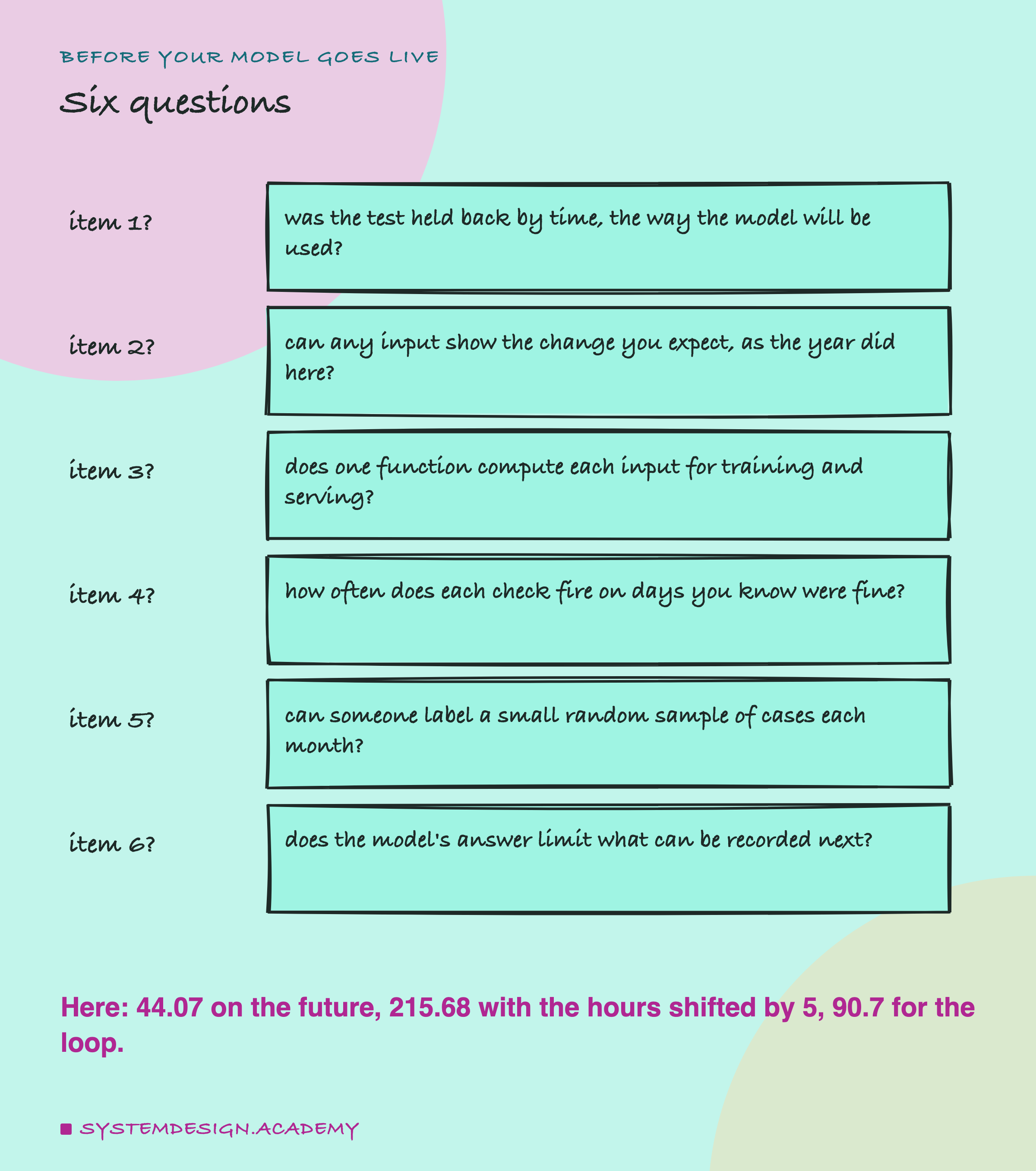
Take one model that you or your team is about to ship, or already runs, and ask the six questions on the card, one at a time. You do not need to answer all of them this week. Start with the first: find the line of code that made the test set. If the rows have a time and it shuffles them, you will learn the number your users are going to see before they see it.

Keep the answers in a file, the way this chapter kept its results. The next time someone asks whether the model is ready, you can point at evidence rather than a feeling. And when something breaks that is not on the list, as it will, measure it and add a line. That is how this list was written.

This is the end of the chapter. The next chapter planned for the course steps back from a single model to the whole life of one: how a model moves from an idea to data, training, release and the watching this chapter measured.