Tokens And Embeddings

Finding Neighbours Fast: Search a Few Clusters Instead of Everything

0 of 13 complete

0%

Contents

Back|Tokens And EmbeddingsFinding Neighbours Fast: Search a Few Clusters Instead of Everything
1/13
36 min left
Prerequisites
Smaller Numbers: Storing Embeddings in One Byte or One Bitrequired
Related Topics
Chunking: The First Lever on Retrieval QualityRetrieval and RAG in ProductionIs There Really a Best Chunk Size? Measured on This Course's Own LessonsRetrieval and RAG in ProductionThe RAG Scale Cliff: What Breaks Between 100 and 5 Million DocumentsRetrieval and RAG in ProductionHybrid Retrieval: When Keyword Search Beats Your EmbeddingsRetrieval and RAG in ProductionThe RAG Retrieval Cliff: Engineering Recall Back at ScaleRetrieval and RAG in Production
1 of 13

Go to the Right Shelf First

When you look for a book in a library, you do not read every book. The books are sorted by subject, so you walk to the right section and look there.

A flat illustration of a librarian in a large library with tall shelves sorted by subject, holding a few books and thinking, beside an empty book trolley. A line says nobody reads every book to find one: you walk to the right section and look there.

Every search in this chapter so far has been exact: the question is compared with every stored piece. That is fine for 1,823 pieces. With millions of pieces, comparing every one for every question is a lot of work, which is why large systems usually avoid it. This lesson measures the library trick: group the pieces first, then search only the nearest groups.

The Words You Need First
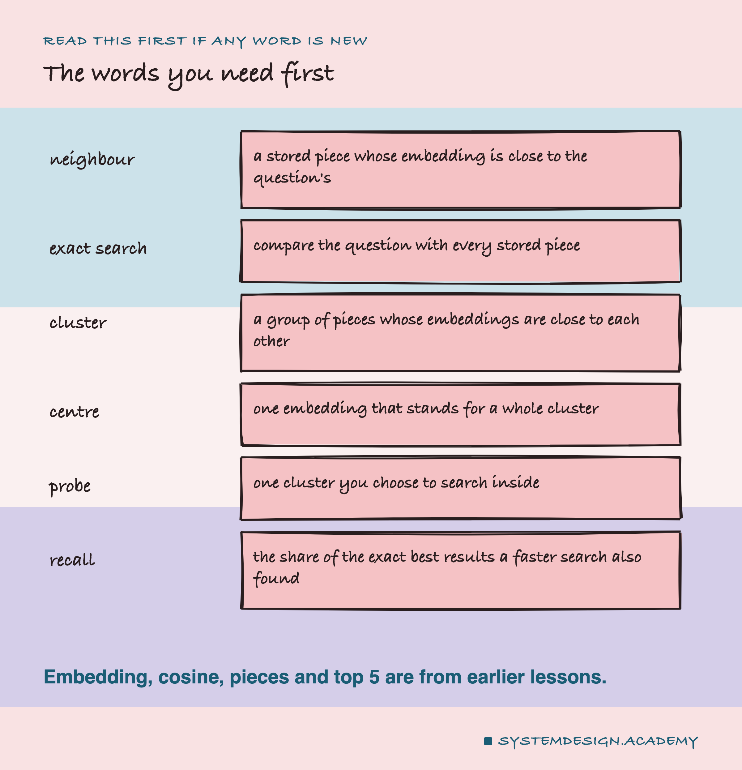
A hand-drawn word list. Neighbour: a stored piece whose embedding is close to the question's. Exact search: compare the question with every stored piece. Cluster: a group of pieces whose embeddings are close to each other. Centre: one embedding that stands for a whole cluster. Probe: one cluster you choose to search inside. Recall: the share of the exact best results a faster search also found. A note says embedding, cosine, pieces and top 5 are from earlier lessons.

Neighbour. A stored piece whose is close to the question's.

Exact search. Compare the question with every stored piece. Nothing is missed, but every piece costs one comparison: one cosine score, as in earlier lessons.

Cluster. A group of pieces whose embeddings are close to each other.

Centre. One embedding that stands for a whole cluster: the average of its pieces, scaled back to length 1.

Probe. One cluster you choose to search inside. More probes means more clusters searched.

Recall. Exact search finds the best results. Recall is the share of those that a faster search also finds. The report below calls it "found exact top 5".

Right lesson. As in lesson 6, each quiz question comes from one lesson, and that lesson is the right answer.

Seed. The number that fixes a random start, so a run can be repeated. Seed 1, 2 and 3 are three different random starts.

Try It: Nine Texts, Three Clusters

This file embeds nine short texts about three topics, groups them into three clusters with a method called k-means (explained two slides on), and then answers one question two ways: by comparing it with all nine, and by comparing it only with the texts in the nearest cluster. Here it is, open in my VS Code.
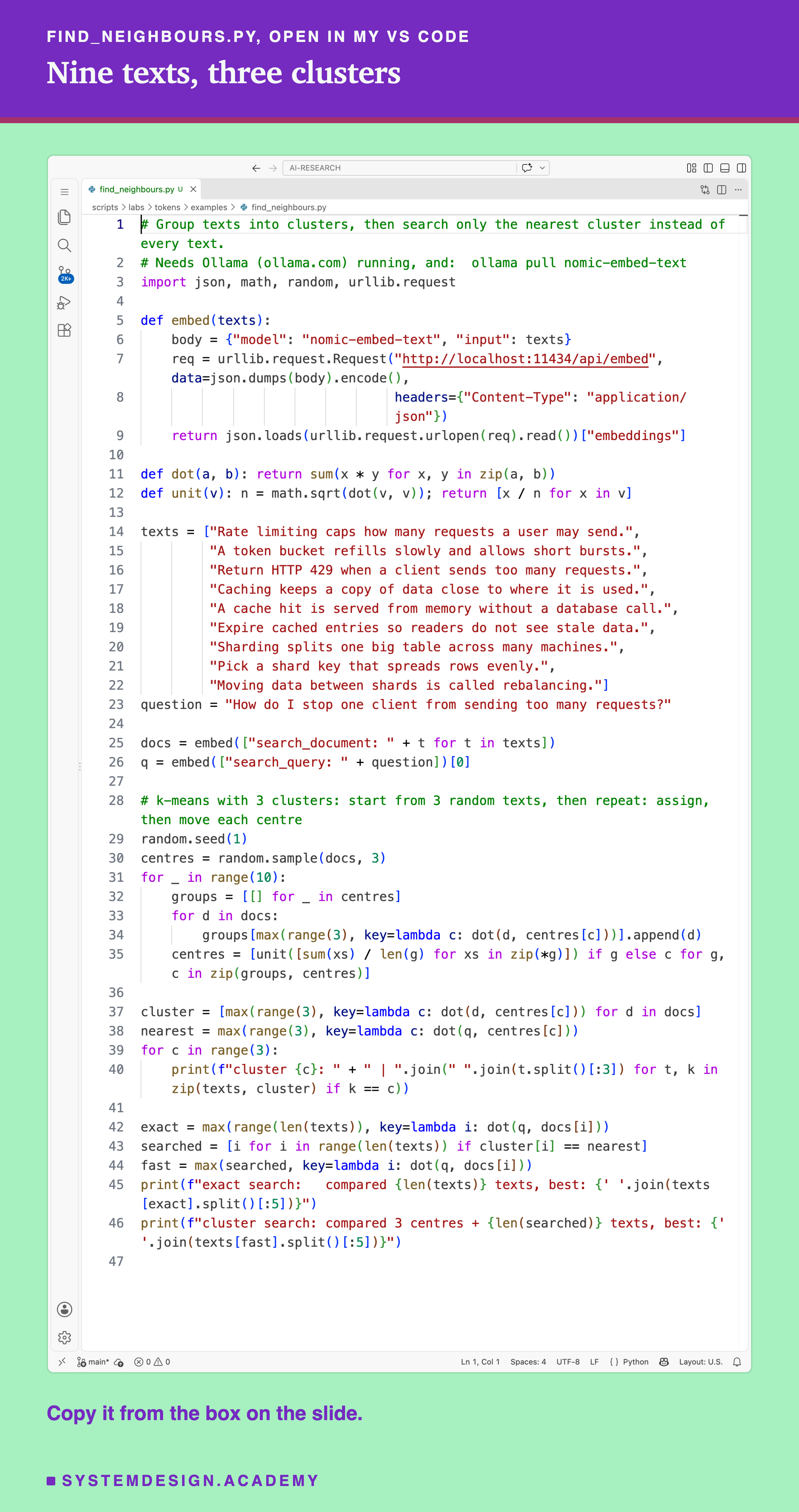
A real screenshot of find_neighbours.py open in VS Code, 47 lines: an embed function using nomic-embed-text through Ollama, dot and unit helpers, nine texts about rate limiting, caching and sharding, a question about a client sending too many requests, a k-means loop with 3 clusters and a random seed of 1 that assigns every text to its nearest centre and moves each centre 10 times, then prints each cluster and compares exact search with cluster search.

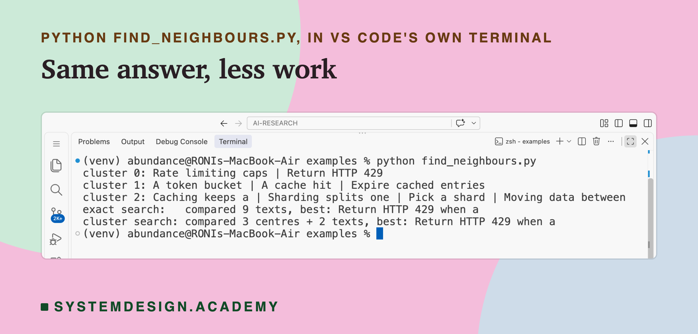
And this is what it printed:

A real screenshot of VS Code's terminal after running python find_neighbours.py. Cluster 0: Rate limiting caps, Return HTTP 429. Cluster 1: A token bucket, A cache hit, Expire cached entries. Cluster 2: Caching keeps a, Sharding splits one, Pick a shard, Moving data between. Exact search compared 9 texts, best: Return HTTP 429 when a. Cluster search compared 3 centres plus 2 texts, best: Return HTTP 429 when a.

Both searches found the same best text. Exact search compared the question with 9 texts. Cluster search compared it with 3 centres and then only the 2 texts in cluster 0.
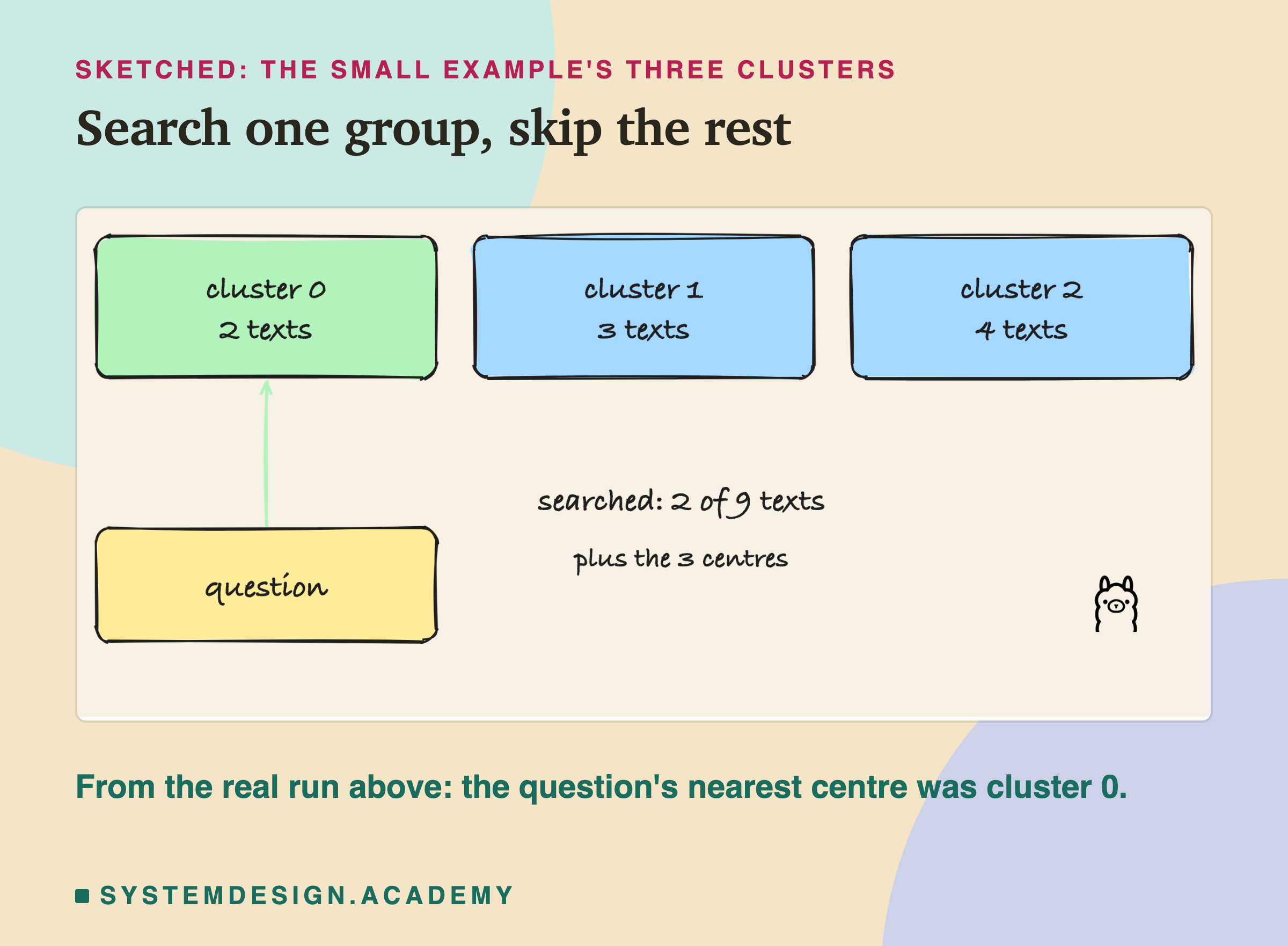
A hand-drawn sketch of the three clusters from the run: cluster 0 with 2 texts, cluster 1 with 3 texts, cluster 2 with 4 texts. An arrow goes from the question to cluster 0 only. A note says searched: 2 of 9 texts, plus the 3 centres. The Ollama logo sits below. A caption says from the real run above, the question's nearest centre was cluster 0.

Look at cluster 1, though. "A token bucket refills slowly and allows short bursts" is about , the very topic of the question. It landed in cluster 1 with two caching texts, so the cluster search never looked at it.
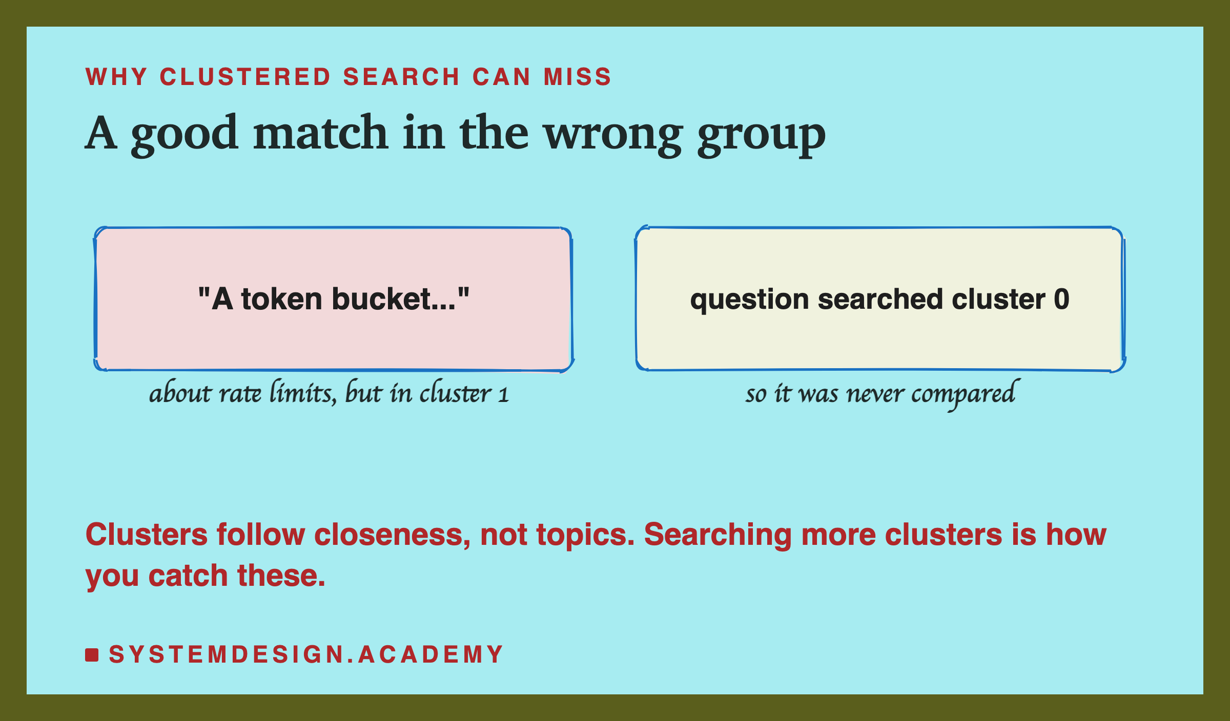
A hand-drawn pair of boxes: "A token bucket...", about rate limits but in cluster 1, and question searched cluster 0, so it was never compared. A note says clusters follow closeness, not topics, and searching more clusters is how you catch these.

Here that did not change the best answer. But it shows the risk: clusters are built from closeness between numbers, not from topics, and a good match can sit in a cluster you skipped.

How Clustered Search Works

Exact search compares the question with every piece, every time.
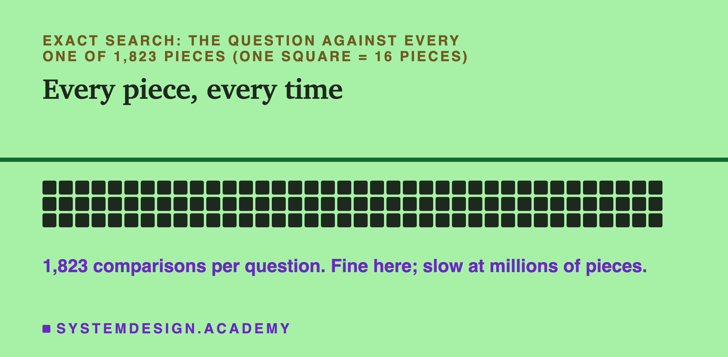
Squares standing for all 1,823 pieces, one square for 16 pieces, all filled. Titled every piece, every time. A note says 1,823 comparisons per question: fine here, slow at millions of pieces.

Clustered search does some work once, before any question arrives. It groups the pieces with a method called k-means:
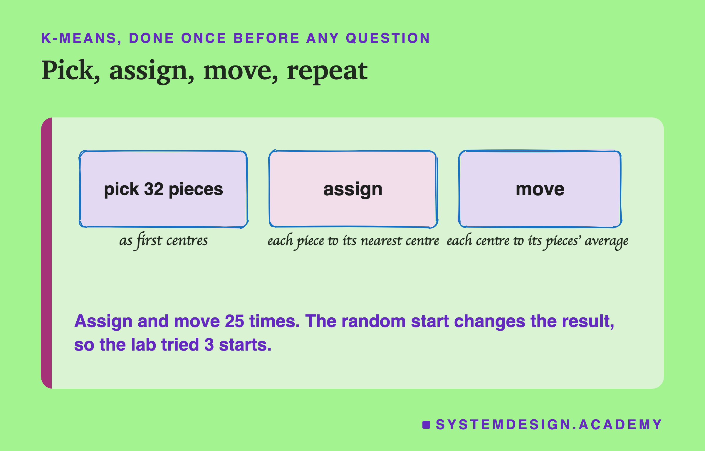
A hand-drawn three-step process: pick 32 pieces as first centres; assign each piece to its nearest centre; move each centre to its pieces' average. A note says assign and move 25 times, and because the random start changes the result, the lab tried 3 starts.

  1. Pick some pieces at random as the first centres. Here, 32 of them.
  2. Assign every piece to its nearest centre.
  3. Move each centre to the average of the pieces now assigned to it.
  4. Repeat assign and move. The lab did it 25 times.

A real 2-D map of all 1,823 pieces, one dot each, coloured by their k-means cluster, 32 colours. The dots overlap heavily. A caption says this is real data, and these 2 directions hold only 9% of the spread, so this flat map cannot show how the clusters separate in the full 768.

That map is the real data, squashed from 768 numbers to 2 so it can be drawn. This flat picture keeps only 9% of the differences between the pieces, which is why the colours look mixed. The clusters are built in the full 768 numbers, not on this map.

Then, for each question:
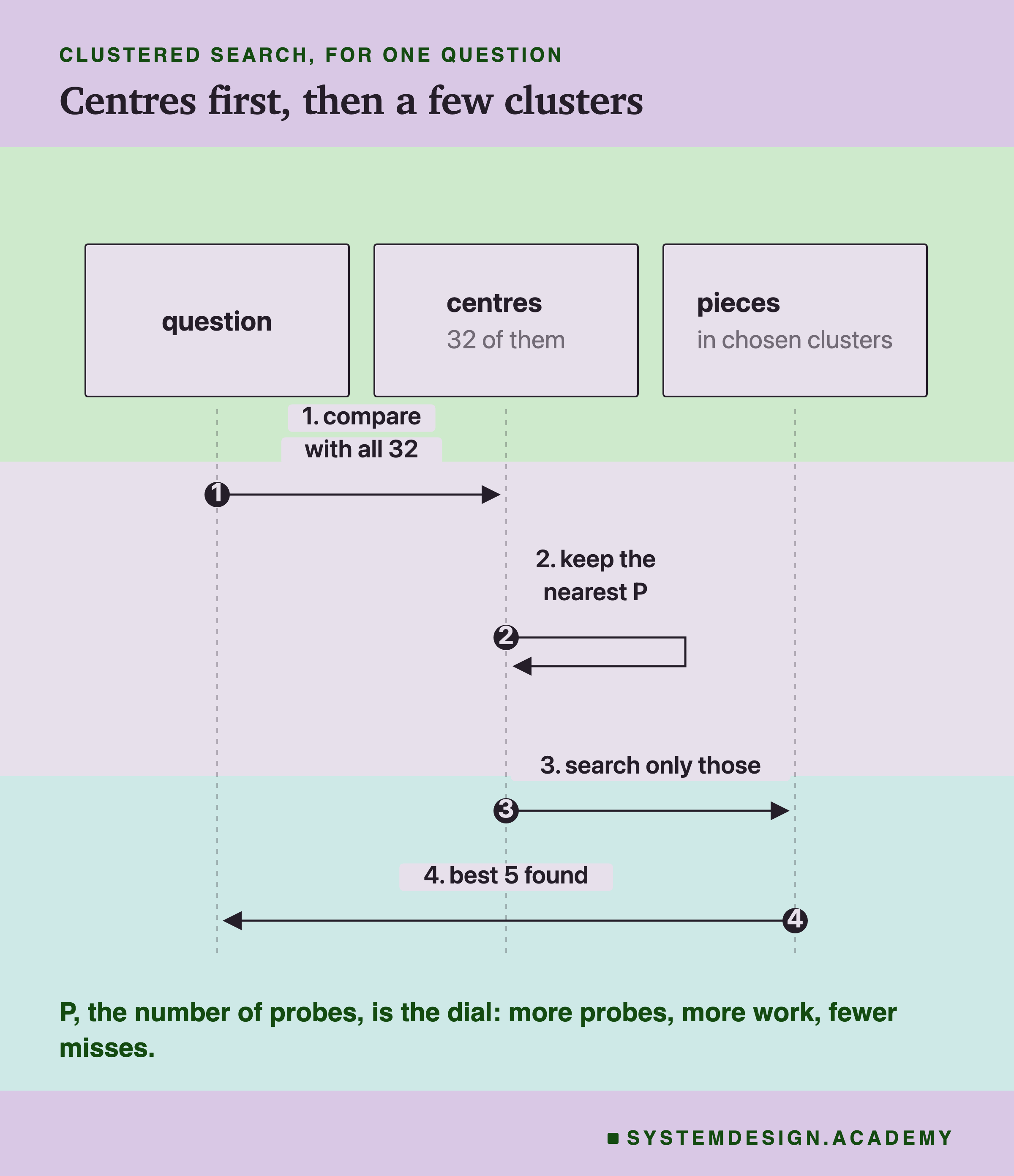
A sequence diagram with three columns: question, centres (32 of them) and pieces in the chosen clusters. Step 1: compare the question with all 32 centres. Step 2: keep the nearest P. Step 3: search only those clusters. Step 4: return the best 5 found. A note says P, the number of probes, is the dial: more probes, more work, fewer misses.

This is called an inverted file index, or IVF. You choose how many clusters to search; that number is called the probes. It is the dial you turn: more probes means more work and fewer misses.

The Real Test
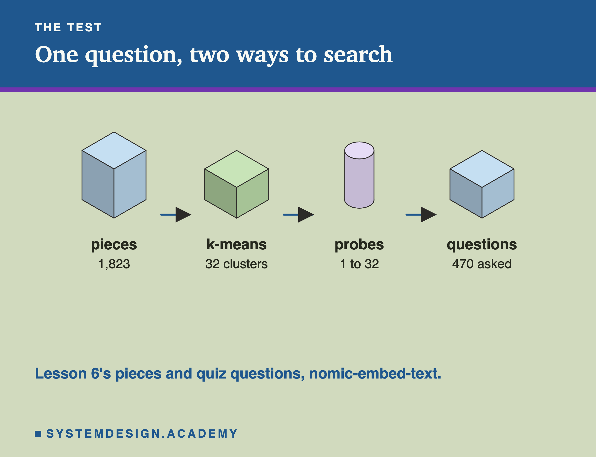
An isometric row of four blocks joined by arrows: 1,823 pieces, k-means into 32 clusters, probes from 1 to 32, and 470 questions asked. A note says these are lesson 6's pieces and quiz questions, with nomic-embed-text.

The same test as lessons 6, 8 and 9:

  • Documents: 1,823 pieces of 200 words from 112 lessons, nomic-embed-text vectors.
  • Questions: the 470 quiz questions inside those lessons.
  • Exact search as the reference.
  • Clustered search with 32 clusters, about 57 pieces each on average, searching 1, 2, 4, 8, 16 or all 32 of them. 32 is a choice for this size, not a rule; with more pieces you would use more clusters.
  • Three random starts for k-means, to see how much luck matters.

The work is counted, not timed. With only 1,823 pieces every search takes a tiny fraction of a second on a laptop, so a timing would say almost nothing. The count of comparisons says exactly how much less work was done. It includes the 32 comparisons with the centres, which is why searching all 32 clusters comes to 102% of exact search.

Here is the lab's report, from the terminal.
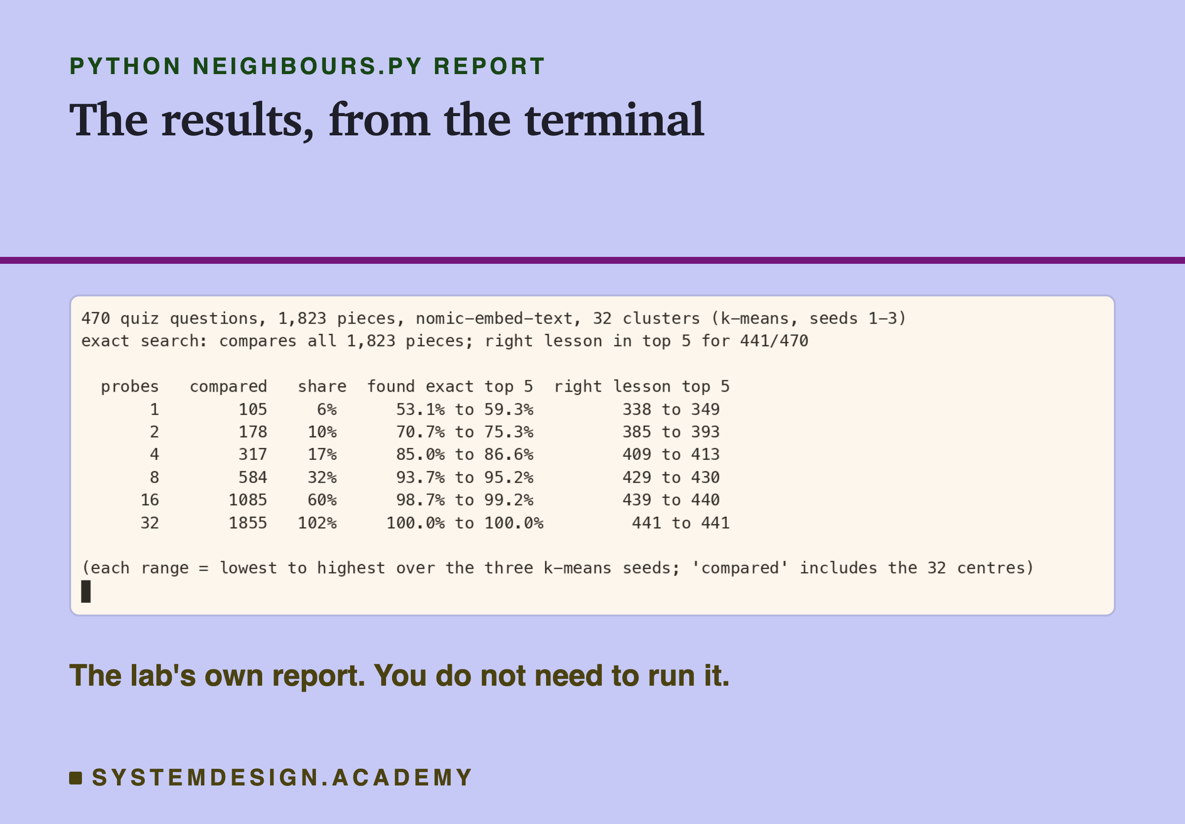
A real terminal recording of neighbours.py's report: 470 quiz questions, 1,823 pieces, nomic-embed-text, 32 clusters, seeds 1 to 3. Exact search compares all 1,823 pieces and finds the right lesson in the top 5 for 441. Probes 1: 105 compared, 6%, found 53.1% to 59.3% of the exact top 5, right lesson 338 to 349. Probes 2: 178, 10%, 70.7% to 75.3%, 385 to 393. Probes 4: 317, 17%, 85.0% to 86.6%, 409 to 413. Probes 8: 584, 32%, 93.7% to 95.2%, 429 to 430. Probes 16: 1085, 60%, 98.7% to 99.2%, 439 to 440. Probes 32: 1855, 102%, 100%, 441.

As a check, exact search found the right lesson in the top 5 for 441, the same as lessons 8 and 9.

Most of the Answer for a Third of the Work
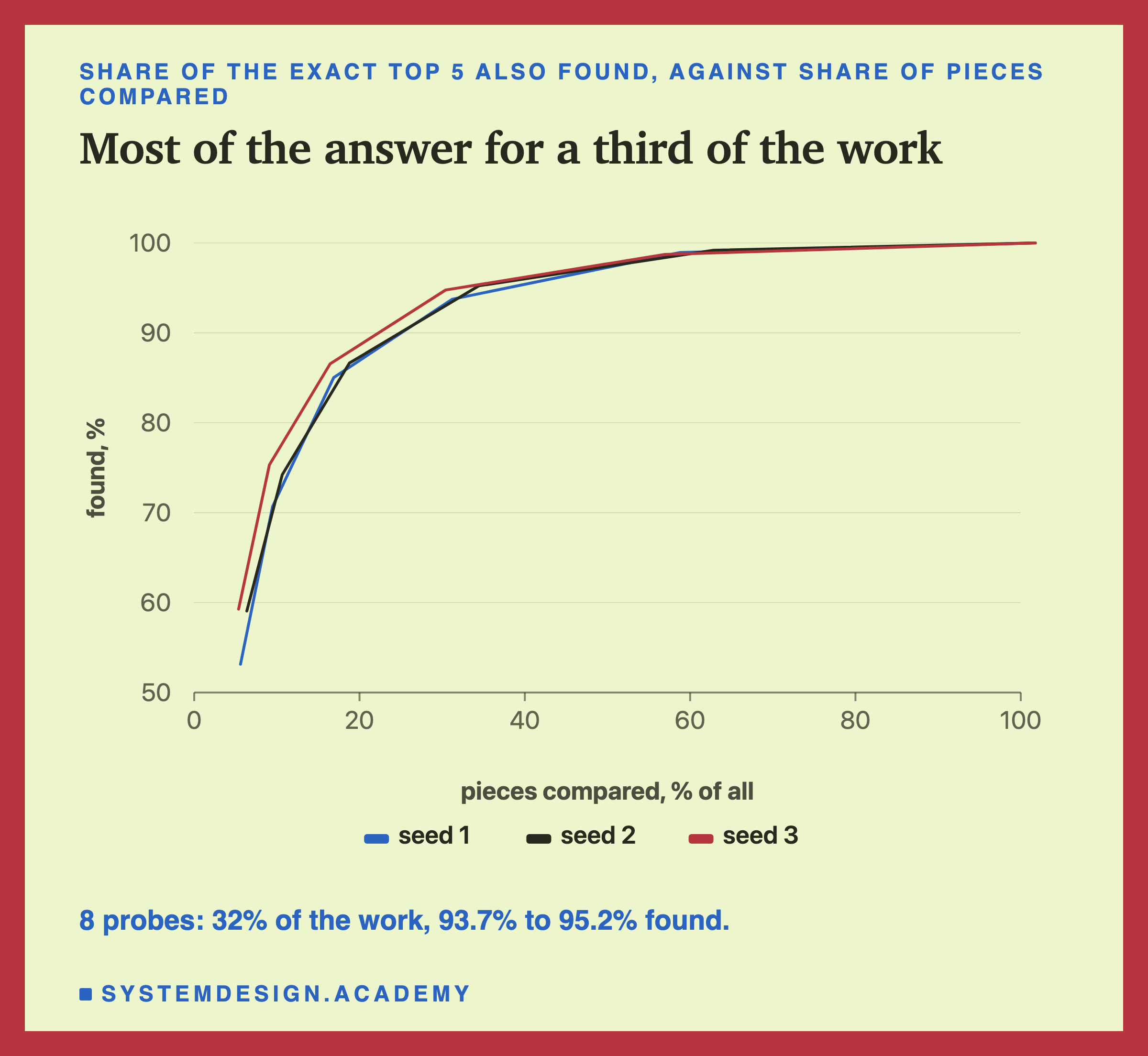
A line chart for three k-means seeds: share of the exact top 5 also found, against pieces compared as a share of all. All three curves rise steeply, from about 53 to 59% at 6% of the work, past 85% at 17%, to about 94 to 95% at 32%, and near 99% at 60%. A note says 8 probes: 32% of the work, 93.7% to 95.2% found.

The curve rises fast and then flattens:

  • 1 cluster of 32: 6% of the comparisons, and 53 to 59% of the exact top 5 found.
  • 8 clusters: 32% of the comparisons, and 94 to 95% found.
  • 16 clusters: 60% of the comparisons, and 99% found.

Each range is the lowest to the highest of the three random starts.
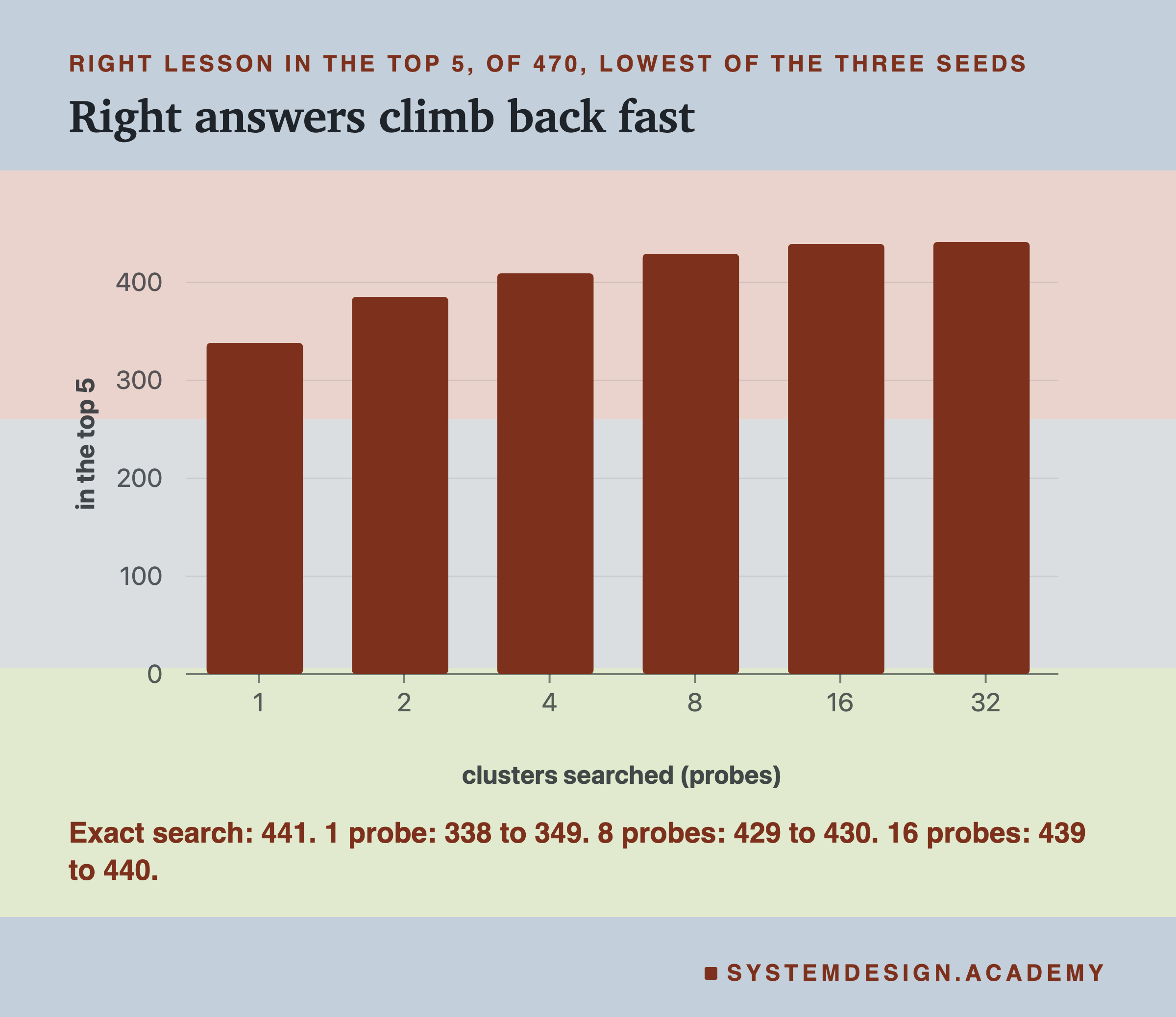
A bar chart of the right lesson in the top 5, of 470, the lowest over the three seeds, at 1, 2, 4, 8, 16 and 32 probes. The bars climb from 338 to 441. A note says exact search 441; 1 probe 338 to 349; 8 probes 429 to 430; 16 probes 439 to 440.

For finding the right lesson, the picture is the same. With 8 probes, 429 to 430 questions still found their lesson in the top 5, against 441 with exact search.
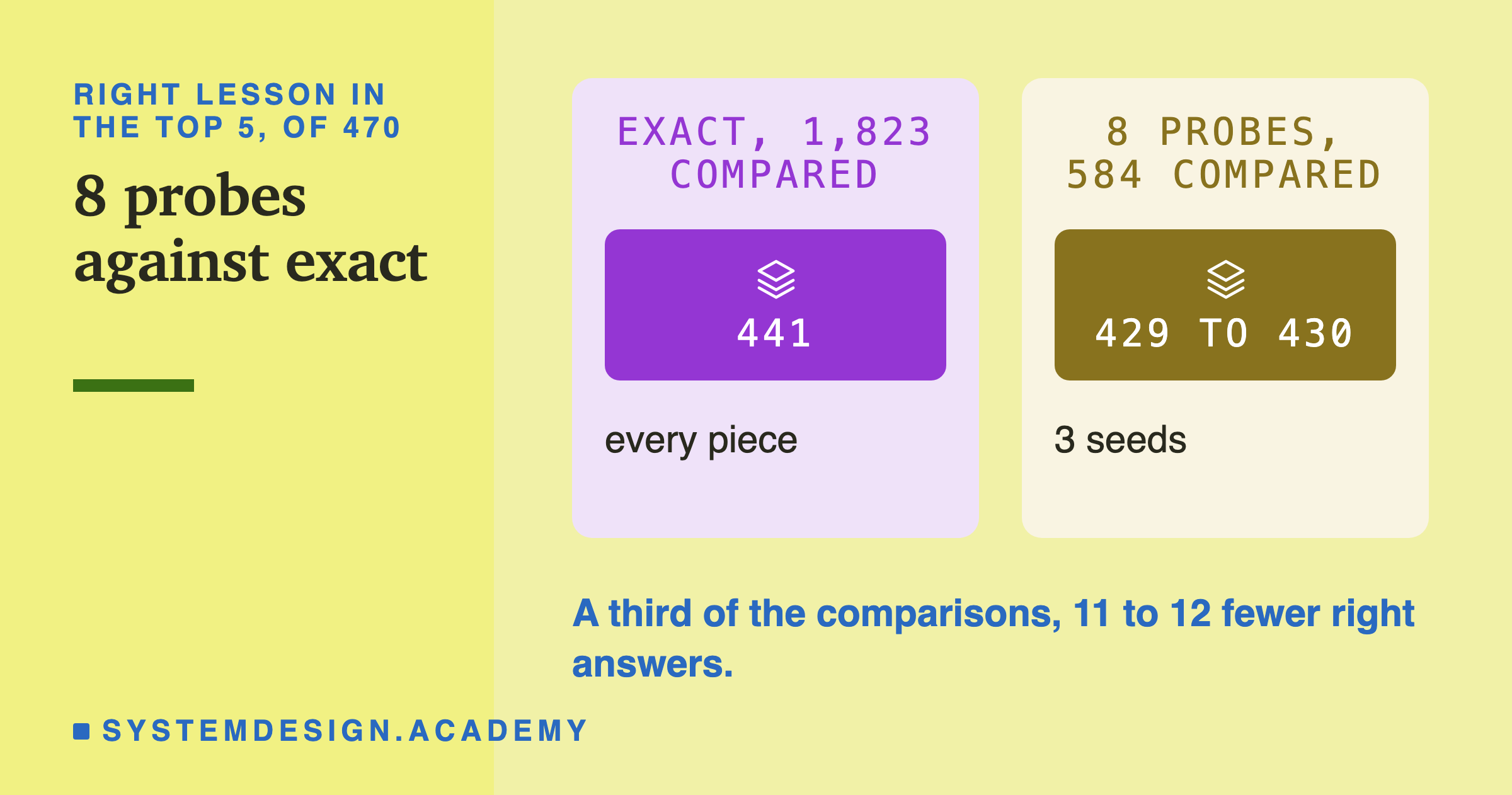
Two panels, right lesson in the top 5 of 470. Exact, 1,823 compared: 441, every piece. 8 probes, 584 compared: 429 to 430, 3 seeds. A note says a third of the comparisons, 11 to 12 fewer right answers.

Why can the right lesson still be found when some of the exact top 5 pieces are missed? Two reasons. A lesson has many pieces, so if its best piece sits in a skipped cluster, another of its pieces may still be searched; its score drops a little, but it can stay in the top 5. And lessons with no piece searched cannot compete at all, which can move the right lesson up.

The Random Start Matters Most When You Search Little
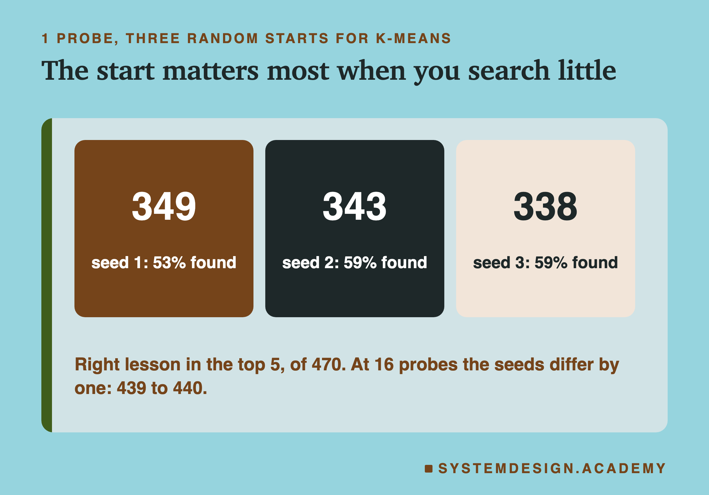
Three boxes for 1 probe, one per k-means seed: seed 1, 349, 53% found; seed 2, 343, 59% found; seed 3, 338, 59% found. A note says right lesson in the top 5 of 470, and at 16 probes the seeds differ by one, 439 to 440.

With only 1 probe, the three random starts gave 349, 343 and 338 right lessons. This is surprising: seed 1 found only 53% of the exact top 5 pieces, but it found the most right lessons. That is the effect from the last slide: finding a lesson needs only one of its pieces, not its best one. With one probe, luck decides a lot. The start decides which pieces end up together, and when you search one small group, that decision matters. With 16 probes, the starts differed by only one question.

What Each Setting Costs
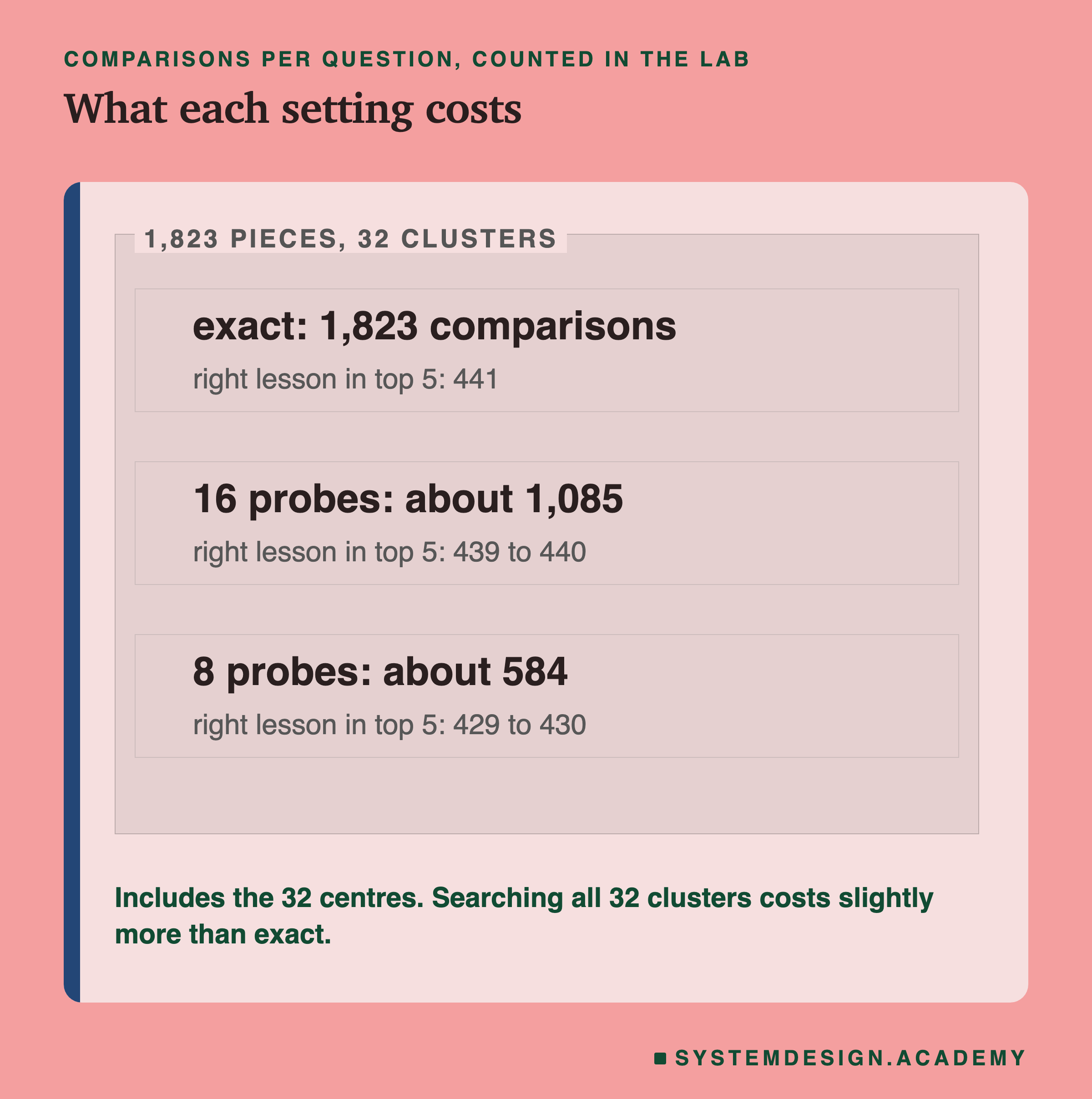
Comparisons per question, counted in the lab, for 1,823 pieces and 32 clusters. Exact: 1,823 comparisons, right lesson in the top 5 441. 16 probes: about 1,085, right lesson 439 to 440. 8 probes: about 584, right lesson 429 to 430. A note says this includes the 32 centres, and searching all 32 clusters costs slightly more than exact.

Notice the last point: searching all 32 clusters costs a little more than exact search, 1,855 against 1,823, because the 32 centres are compared as well. Clustered search only pays off when you search a fraction of the clusters.

Count It Yourself

This box holds the real ranks from the test, for seed 1: for each of the 470 questions, which place the right lesson got (112, the last place, means it was not found at all), with exact search and with 1, 4, 8 or 16 clusters searched. Press Run. Then change PROBES to "1" or "16", and TOP to 1.

When to Use Clustered Search
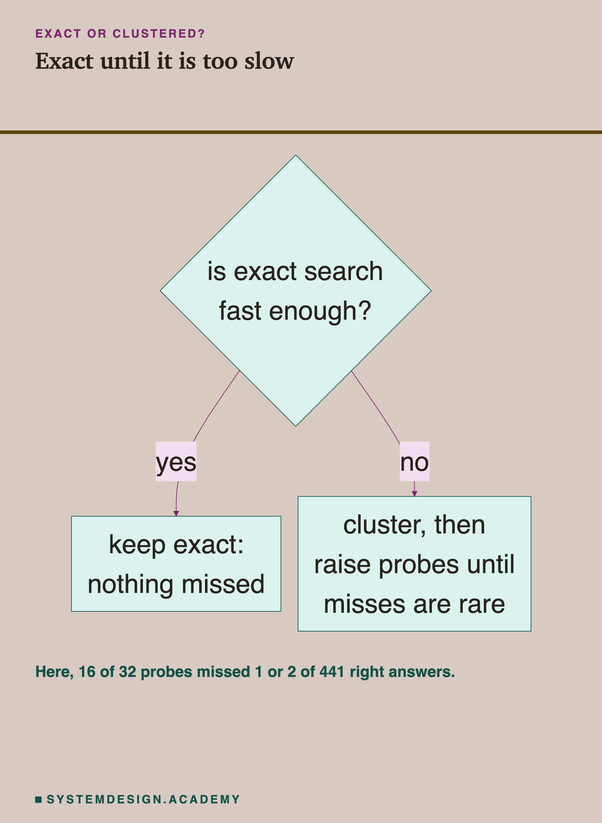
A flowchart: is exact search fast enough? If yes, keep exact: nothing missed. If no, cluster, then raise probes until misses are rare. A note says here 16 of 32 probes missed 1 or 2 of 441 right answers.

  1. Start with exact search. It never misses. This lesson did not time anything, so time it yourself on your own data.
  2. When it becomes too slow for you, for example when answers take longer than your users will wait, switch to a clustered or other approximate method. Approximate means it may miss a few results in exchange for less work.
  3. Turn the dial: raise the number of clusters searched until the misses are few enough for you. Here, 16 of 32 missed 1 or 2 of 441 right lessons.
  4. Always measure against exact search. Exact is the reference that tells you what the shortcut costs.

Vector databases (databases built to store and search them) offer several fast search methods. The clustered one in this lesson is often called IVF. Another common one, HNSW, links each piece to a few of its near neighbours, like a map of roads between them, and walks along those links towards the question. This lesson did not test HNSW.
Two cards with logos: Ollama running nomic-embed-text, and NumPy doing k-means and search. A note says it is free and local, with no search library.

What This Lesson Measured, and What It Did Not
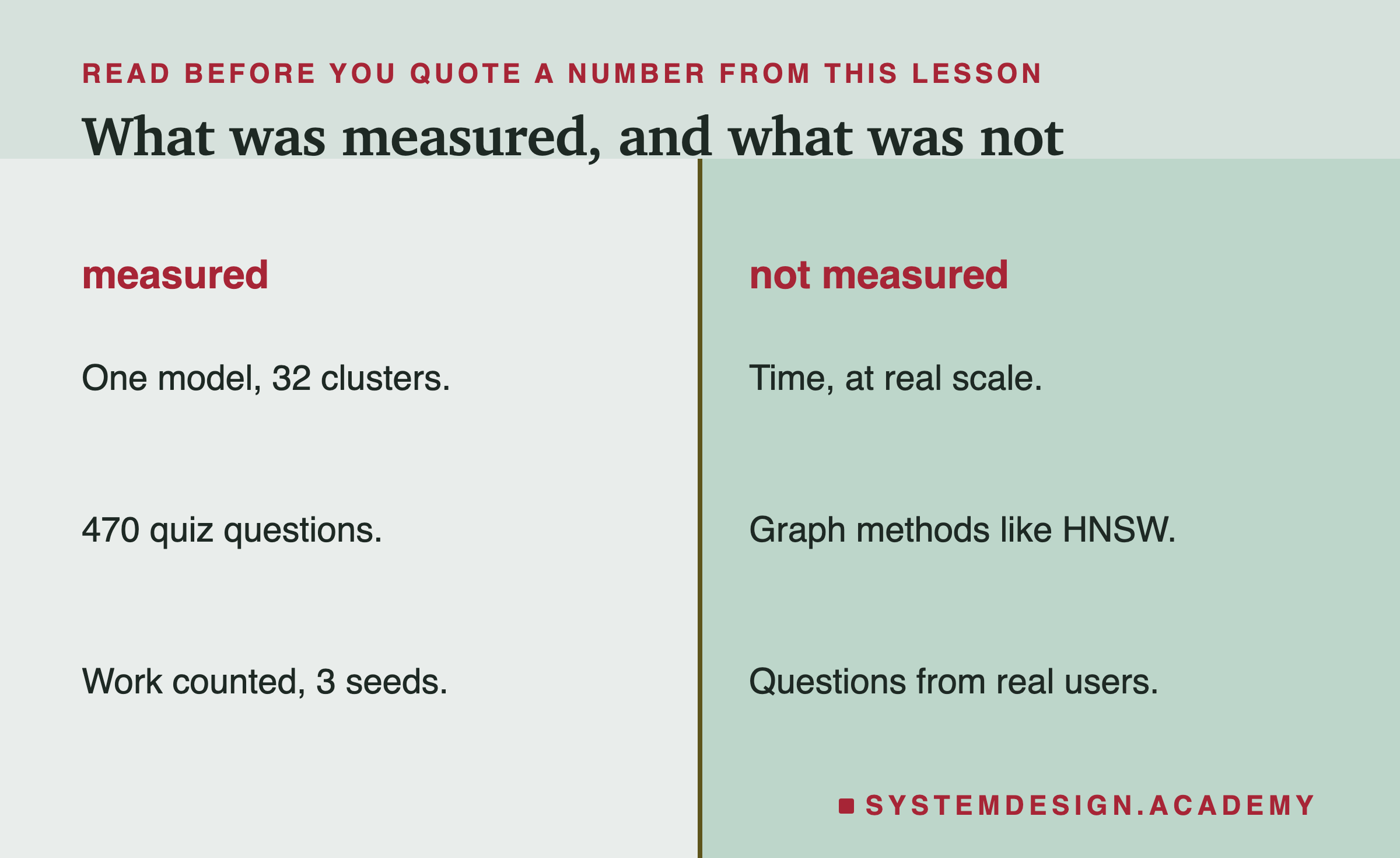
Two columns. Measured: one model with 32 clusters, 470 quiz questions, work counted over 3 seeds. Not measured: time at real scale, graph methods like HNSW, questions from real users.

Measured: one model, 32 clusters, three random starts, 470 quiz questions over 1,823 pieces. Work was counted as comparisons, exactly.

Not measured: time, other numbers of clusters, graph methods like , and questions from real users. At millions of pieces the numbers would change, and a real database adds its own costs, such as reading from disk.

What to Do Next
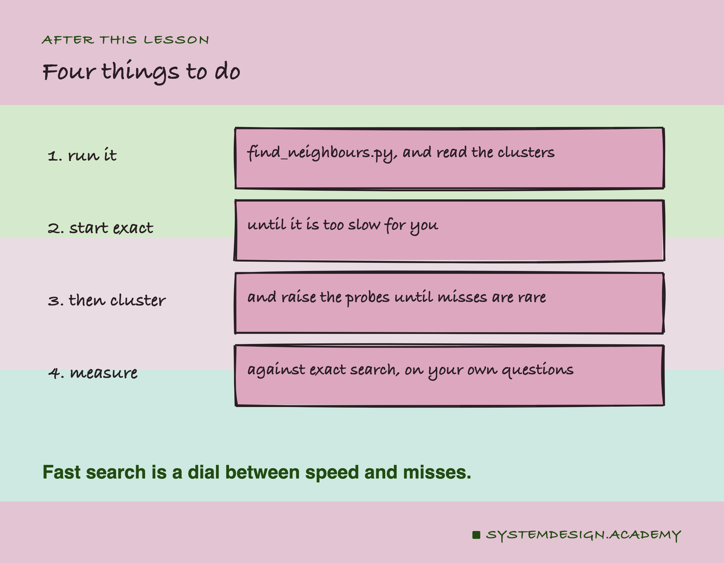
A hand-drawn list of four things to do: run find_neighbours.py and read the clusters; start exact until it is too slow; then cluster and raise the probes until misses are rare; and measure against exact search on your own questions. A note says fast search is a dial between speed and misses.

  1. Run find_neighbours.py and read which texts landed together.
  2. Start with exact search, until it is too slow for you.
  3. Then cluster, and raise the probes until misses are rare.
  4. Measure against exact search, on your own questions.
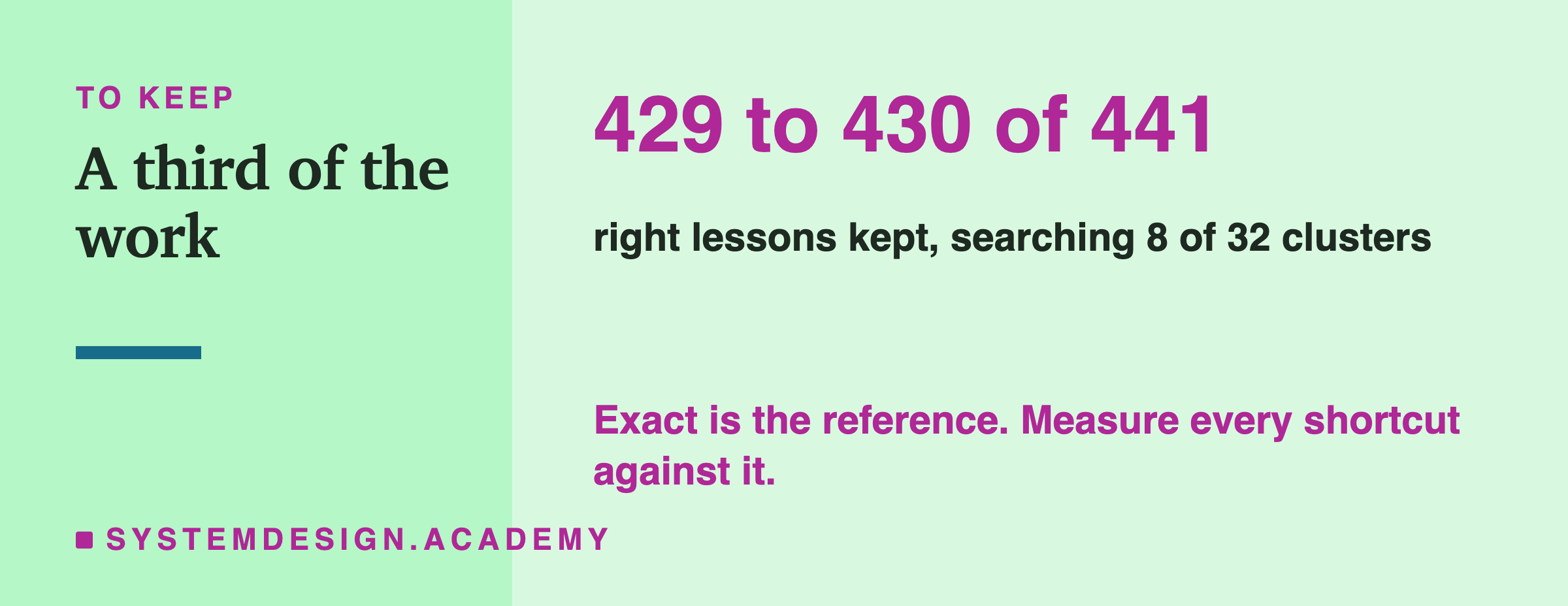
The number to keep: 429 to 430 of 441, right lessons kept searching 8 of 32 clusters. A note says exact is the reference: measure every shortcut against it.

Knowledge Check

Knowledge Check

5 questions - Score 80% to pass

Q1

What does clustered search do differently from exact search?

Q2

Searching 8 of 32 clusters compared about a third of the pieces. How many of the exact top 5 pieces did it still find?

Q3

In the small example, the token bucket text was about rate limits but was never compared with the question. Why?

Q4

With 1 probe, three random starts gave 349, 343 and 338 right lessons. With 16 probes, 439 or 440. What does that show?

Q5

Searching all 32 clusters compared 1,855 pieces and centres, against 1,823 for exact search. What is the lesson?

To run it: install Ollama from ollama.com, open it and leave it running. Run ollama pull nomic-embed-text, save the file below as find_neighbours.py, and run python3 find_neighbours.py (on Windows: python find_neighbours.py). If you see "Connection refused", open the Ollama app first.

# Group texts into clusters, then search only the nearest cluster instead of every text.
# Needs Ollama (ollama.com) running, and:  ollama pull nomic-embed-text
import json, math, random, urllib.request

def embed(texts):
    body = {"model": "nomic-embed-text", "input": texts}
    req = urllib.request.Request("http://localhost:11434/api/embed", data=json.dumps(body).encode(),
                                 headers={"Content-Type": "application/json"})
    return json.loads(urllib.request.urlopen(req).read())["embeddings"]

def dot(a, b): return sum(x * y for x, y in zip(a, b))
def unit(v): n = math.sqrt(dot(v, v)); return [x / n for x in v]

texts = ["Rate limiting caps how many requests a user may send.",
         "A token bucket refills slowly and allows short bursts.",
         "Return HTTP 429 when a client sends too many requests.",
         "Caching keeps a copy of data close to where it is used.",
         "A cache hit is served from memory without a database call.",
         "Expire cached entries so readers do not see stale data.",
         "Sharding splits one big table across many machines.",
         "Pick a shard key that spreads rows evenly.",
         "Moving data between shards is called rebalancing."]
question = "How do I stop one client from sending too many requests?"

docs = embed(["search_document: " + t for t in texts])
q = embed(["search_query: " + question])[0]

# k-means with 3 clusters: start from 3 random texts, then repeat: assign, then move each centre
random.seed(1)
centres = random.sample(docs, 3)
for _ in range(10):
    groups = [[] for _ in centres]
    for d in docs:
        groups[max(range(3), key=lambda c: dot(d, centres[c]))].append(d)
    centres = [unit([sum(xs) / len(g) for xs in zip(*g)]) if g else c for g, c in zip(groups, centres)]

cluster = [max(range(3), key=lambda c: dot(d, centres[c])) for d in docs]
nearest = max(range(3), key=lambda c: dot(q, centres[c]))
for c in range(3):
    print(f"cluster {c}: " + " | ".join(" ".join(t.split()[:3]) for t, k in zip(texts, cluster) if k == c))

exact = max(range(len(texts)), key=lambda i: dot(q, docs[i]))
searched = [i for i in range(len(texts)) if cluster[i] == nearest]
fast = max(searched, key=lambda i: dot(q, docs[i]))
print(f"exact search:   compared {len(texts)} texts, best: {' '.join(texts[exact].split()[:5])}")
print(f"cluster search: compared 3 centres + {len(searched)} texts, best: {' '.join(texts[fast].split()[:5])}")