Data Engineering For Ml

Data Validation and Quality: Stopping Garbage Before It Reaches the Model

0 of 26 complete

0%

Contents

Back|Data Engineering For MlData Validation and Quality: Stopping Garbage Before It Reaches the Model
1/26
88 min left
  1. Home
  2. AI Engineering: Data, RAG and Agents
  3. Data Engineering for ML
  4. Data Validation and Quality: Stopping Garbage Before It Reaches the Model
Prerequisites
Data Lakes, Warehouses, and Lakehouses for MLrequired
Related Topics
Failing Silently: Which Checks Catch a Broken Input Before the Answers ArriveWhy Production BreaksTomorrow Is Different: A Model Frozen on 2011, Scored Through 2012Why Production BreaksTrain/Serve Skew: One Input Computed Two WaysWhy Production BreaksWatching Inputs Before the Answers Arrive: Drift Measures Against the Real ErrorWhy Production BreaksA Production Readiness Check: Everything This Chapter Broke, in the Order You Would Check ItWhy Production Breaks
1 of 26
Previous lesson
Data Lakes, Warehouses, and Lakehouses for ML
Next lessonData Versioning: Reproducing the Exact Data That Trained a Model

System Design

  • Foundation
  • Intermediate
  • Advanced
  • Capstone

AI Engineering

  • Foundation
  • Data, RAG and Agents
  • Evaluation, LLM Ops and Security

systemdesign.academy

  • Home
  • Glossary
  • Interview prep
  • Reviews
  • About
  • Privacy
  • Terms

The Shopping Bag on the Kitchen Table

When I bring a bag of shopping home, I check it on the kitchen table before anything goes into the fridge. I do not think of it as checking. It just happens.

I count the eggs, because the box should hold six. I look for a cracked one. I read the date on the milk. Each check takes a second, and each one looks for one kind of problem. Counting the eggs will never find a crack. Reading the date will never find a missing egg.

An illustration of a woman carrying a shopping bag on her shoulder, standing beside text. Headed the shopping bag on the kitchen table, titled check it before it goes in the fridge. Beside her: each quick check looks for one kind of problem; count the eggs, look for a cracked one, read the date on the milk; too fussy, and good food goes in the bin; too quick, and a bad egg reaches the pan; and milk left warm for an hour in the shop looks like any other milk. Beneath: in this lesson the bag is a day of weather readings, 24 rows; over 730 days, a strict set of checks set aside 37 good days, and no check fired on a thermometer reading 3 degrees high more often than on a good day.

How careful should I be? If I throw away every egg with a speck of dirt on it, I will throw away good food every week. If I only glance at the bag, one day a bad egg will end up in the pan. There is a cost on both sides, and I cannot make both of them zero.

There is also a problem no check on the table can find. Milk that sat warm in the shop for an hour looks exactly like good milk. The date is right, the bottle is sealed, and it is the right size. Only a thermometer in the shop could have told me.

Where This Lesson Starts

A machine learning model is the cook in that kitchen. It uses whatever reaches it, and it cannot tell a good number from a bad one. Nothing crashes when bad data arrives. The model gives an answer, the answer is wrong, and nobody is told.

This lesson is about the checks that stand between new data and the model. The chapter's second lesson, data ingestion pipelines, already built six checks on the table itself: row counts, copies, missing keys, key order, column names and empty columns. Its lab measured them, and I will not repeat that here.
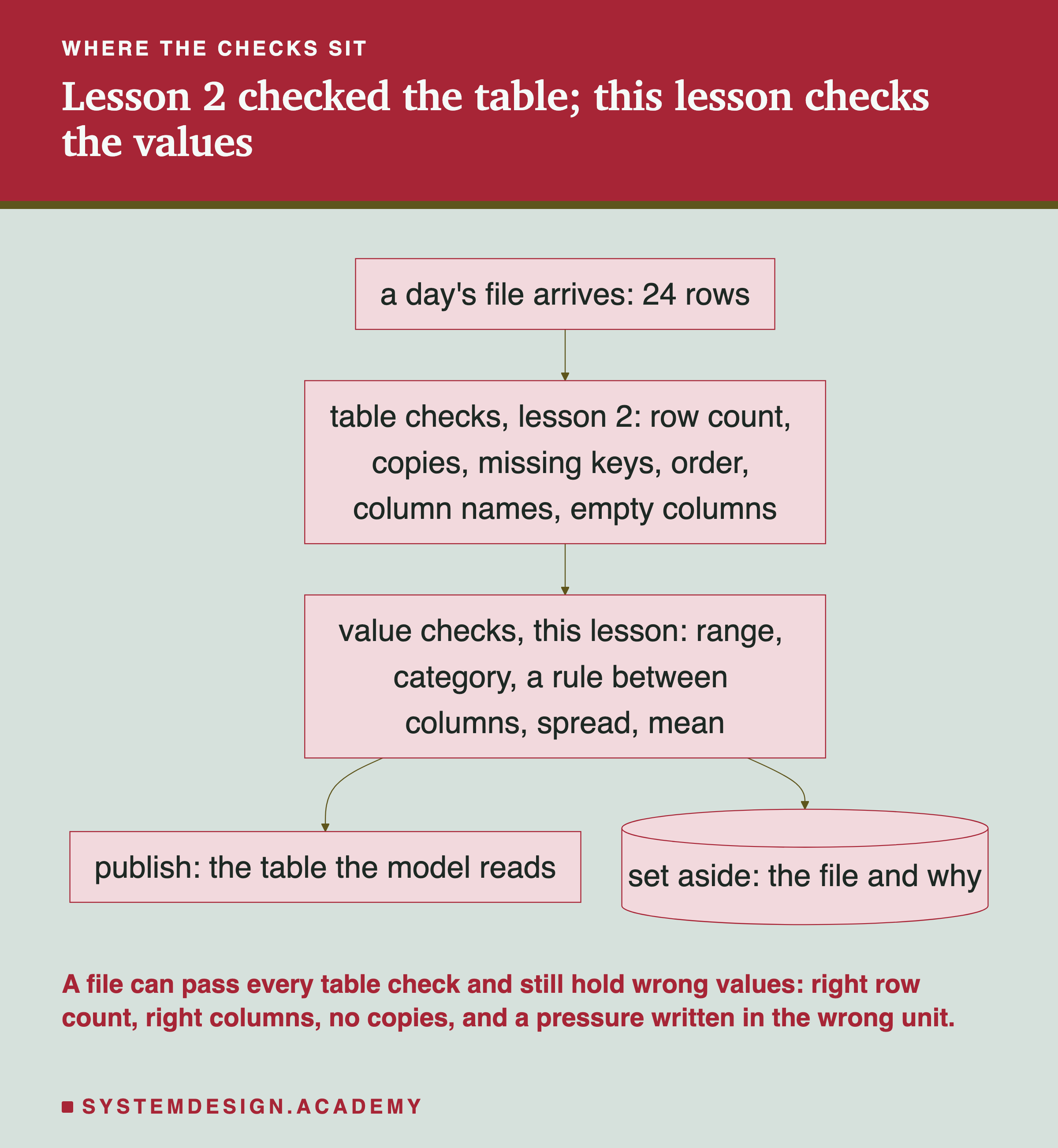
A flowchart headed where the checks sit, titled lesson 2 checked the table; this lesson checks the values. A box, a day's file arrives: 24 rows, leads to a box, table checks, lesson 2: row count, copies, missing keys, order, column names, empty columns. That leads to a box, value checks, this lesson: range, category, a rule between columns, spread, mean. That splits into two: a box, publish: the table the model reads; and a cylinder, set aside: the file and why. Beneath: a file can pass every table check and still hold wrong values: right row count, right columns, no copies, and a pressure written in the wrong unit.

Lesson 2 ended by saying a pipeline also needs checks on the range and spread of each column. That is where this lesson starts. A file can have the right number of rows, the right columns and no copies, and still carry a pressure written in the wrong unit.

Here is the plan. First, the words, and six ways data can be wrong. Then the gate, which decides what happens to a batch that fails. Then two real tools, run on real data. Then the lab: five years of real weather readings, six faults I put in on purpose, and eight checks. I counted both kinds of mistake a check can make, and what each fault did to a model. After that come drift, real teams, and when a check earns its place.

Twelve Words for This Lesson
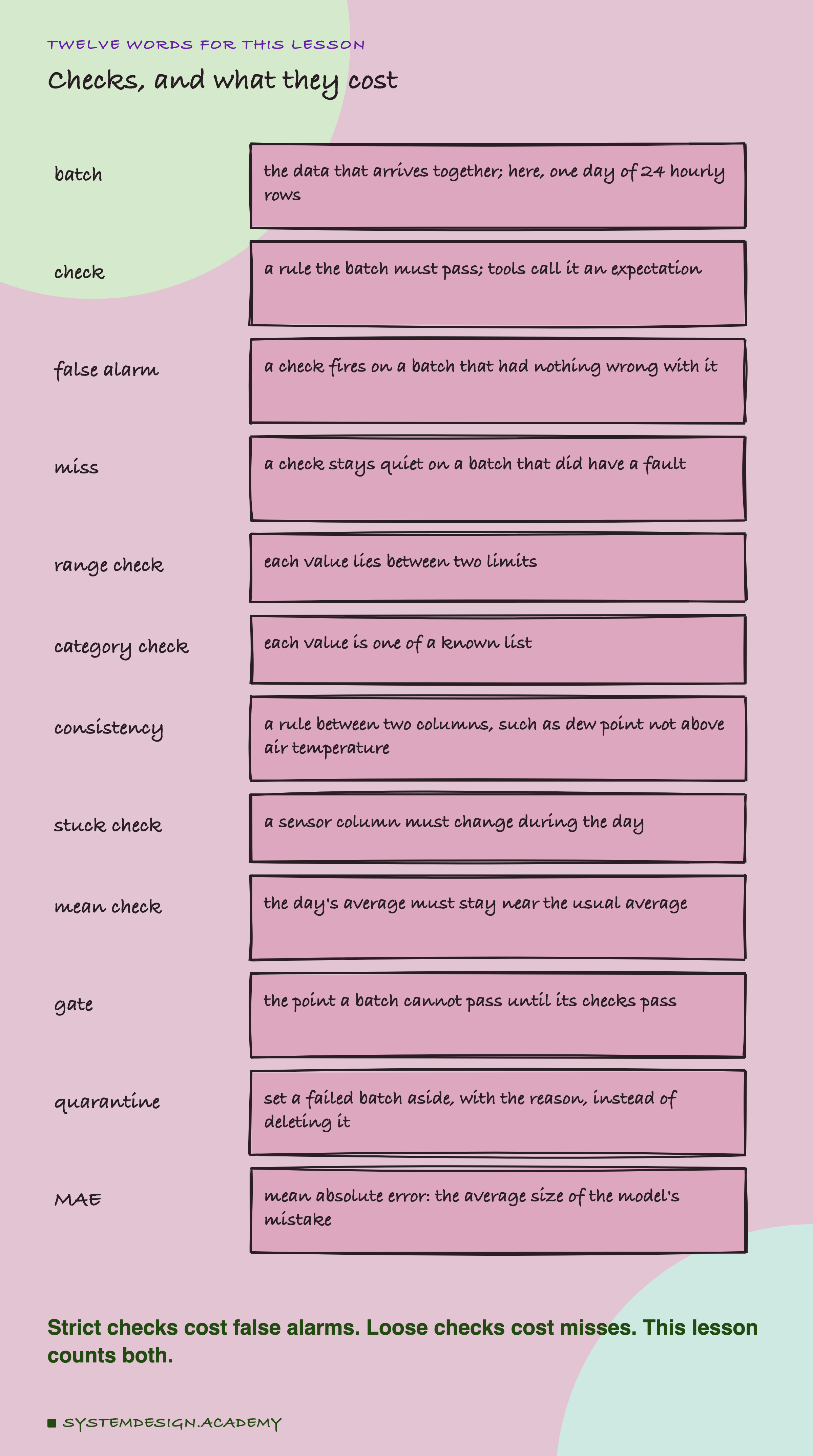
A hand-drawn list headed twelve words for this lesson, titled checks, and what they cost. Batch: the data that arrives together; here, one day of 24 hourly rows. Check: a rule the batch must pass; tools call it an expectation. False alarm: a check fires on a batch that had nothing wrong with it. Miss: a check stays quiet on a batch that did have a fault. Range check: each value lies between two limits. Category check: each value is one of a known list. Consistency: a rule between two columns, such as dew point not above air temperature. Stuck check: a sensor column must change during the day. Mean check: the day's average must stay near the usual average. Gate: the point a batch cannot pass until its checks pass. Quarantine: set a failed batch aside, with the reason, instead of deleting it. MAE: mean absolute error, the average size of the model's mistake. Beneath: strict checks cost false alarms; loose checks cost misses; this lesson counts both.

A batch is the data that arrives together. Here one batch is one day of weather: 24 rows, one for each hour. A check is a rule the batch must pass. Great Expectations, one of the tools in this lesson, calls a check an expectation.

A check can be wrong in two ways. A false alarm is when it fires on a batch that had nothing wrong with it. A miss is when it stays quiet on a batch that did have a fault. A strict check has more false alarms. A loose check has more misses.

A range check asks whether each value lies between two limits. A category check asks whether each value is one of a known list. A consistency check is a rule between two columns. A stuck check asks whether a sensor's readings change at all during the day. A mean check asks whether the day's average stays near the usual average.

A gate is the point a batch cannot pass until its checks pass. To quarantine a batch is to set it aside, with the reason it failed, instead of deleting it. MAE, mean absolute error, is the average size of a model's mistake, in the units of what it predicts.

Six Questions About Quality

"Data quality" sounds vague until you split it into questions you can answer. A common list has six, and a batch can pass five of them and still be ruined by the sixth.
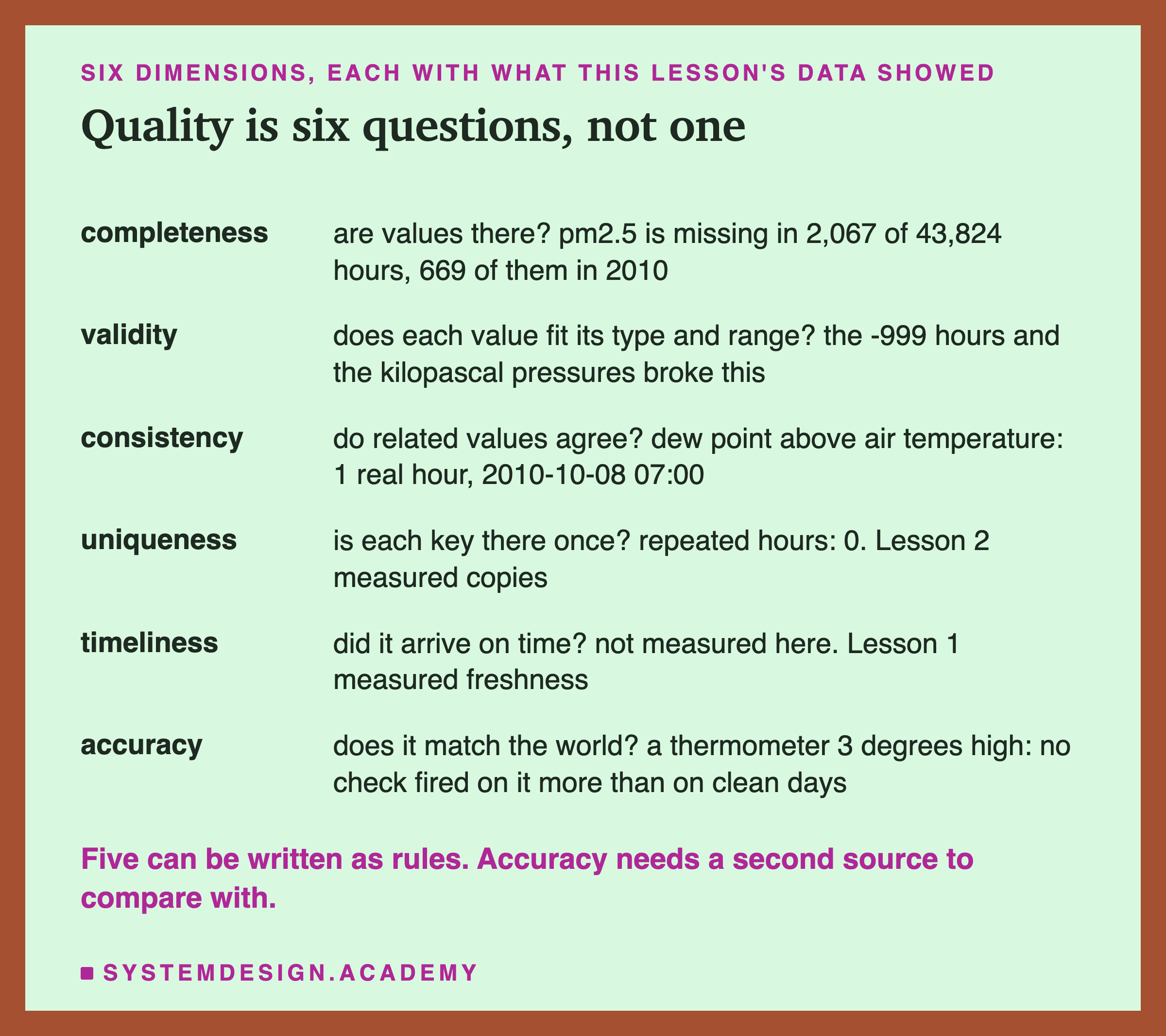
A table headed six dimensions, each with what this lesson's data showed, titled quality is six questions, not one. Completeness: are values there? pm2.5 is missing in 2,067 of 43,824 hours, 669 of them in 2010. Validity: does each value fit its type and range? the -999 hours and the kilopascal pressures broke this. Consistency: do related values agree? dew point above air temperature: 1 real hour, 2010-10-08 07:00. Uniqueness: is each key there once? repeated hours: 0; lesson 2 measured copies. Timeliness: did it arrive on time? not measured here; lesson 1 measured freshness. Accuracy: does it match the world? a thermometer 3 degrees high: no check fired on it more than on clean days. Beneath: five can be written as rules; accuracy needs a second source to compare with.

Completeness asks whether the values are there. The lab's data is real, and it has gaps: the fine-dust reading is missing in 2,067 of 43,824 hours, 669 of them in 2010. PM2.5 is what the model predicts, so the lab simply leaves those hours out: the model learns from 24,418 reference hours and is scored on 17,339 serving hours. When an input column has gaps instead, a model can learn that "missing" means something, and a sudden rise in gaps changes its answers.

Validity asks whether each value fits its type and range. A temperature of -999 is not a temperature. It is a code some feeds use for "no reading". A value like that, which stands in for "no value", is called a sentinel. Consistency asks whether related values agree. Dew point is the temperature at which the air would start to form dew. The US National Weather Service says it "can never be greater than the air temperature". The real data broke that rule once, on 8 October 2010 at 07:00.

Uniqueness asks whether each key appears once. Timeliness asks whether the data came on time. Lessons 1 and 2 of this chapter measured those two, so this lab does not.

Accuracy asks whether a value matches the world. It is the hardest, because a value can be present, valid, consistent and unique, and still be wrong. No rule can see that. You need a second source to compare against. In the lab, a thermometer that read 3 degrees high set off no check more often than a good day did.

Validation Is a Gate, Not a Report

The most common setup I see is a check that writes a report after the data has already landed. By the time anyone reads it, the bad rows are in the table, and a model may have trained on them. A check you do not act on is only a comment.

A gate works the other way round. New data lands somewhere private first. The checks run there. Only a batch that passes is published to the table that models and dashboards read.
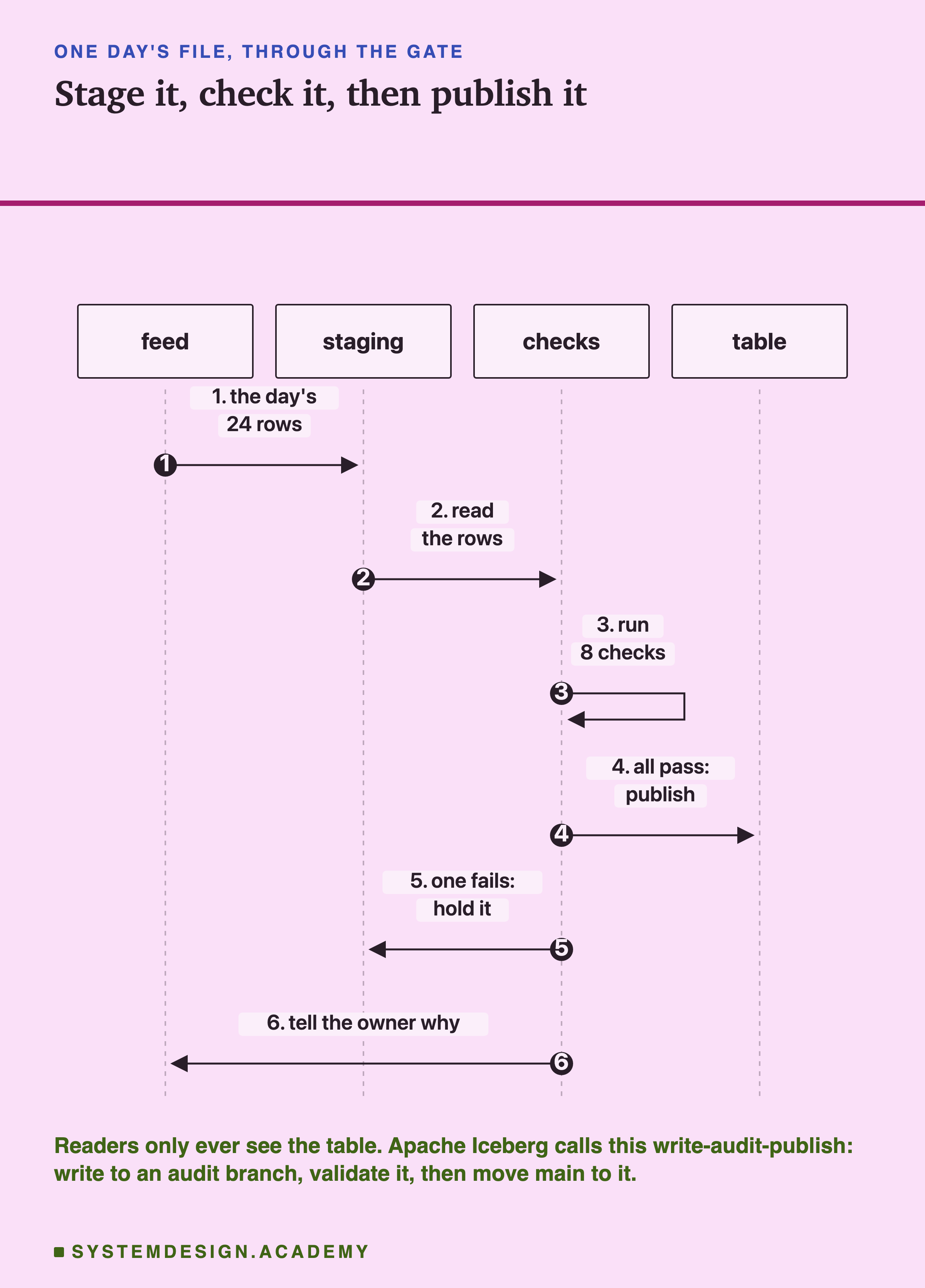
A sequence diagram with four columns, feed, staging, checks and table, headed one day's file, through the gate, titled stage it, check it, then publish it. Step 1, the feed sends staging the day's 24 rows. Step 2, the checks read the rows. Step 3, the checks run 8 checks on themselves. Step 4, all pass: the checks publish to the table. Step 5, one fails: the checks hold it in staging. Step 6, the checks tell the feed's owner why. Beneath: readers only ever see the table; Apache Iceberg calls this write-audit-publish: write to an audit branch, validate it, then move main to it.

This pattern has a name: write-audit-publish. Michelle Ufford's 2017 talk on data quality at Netflix listed it as an "ETL pattern for high-quality big data jobs". The Apache Iceberg table format builds it in. Its documentation says "writes are performed on a separate audit-branch independent from the main table history". After validation, "the main branch can be fastForward to the head of audit-branch". A branch here is a separate line of versions of the table, like a branch in Git: writes go to it without touching the main one. Fast-forward just means main now points at the checked data.

Why put the gate at the data layer, and not inside each model? Because one gate protects every reader of the table: this model, the next model, and every dashboard. Checks written inside each apart over time. And the day a new reader appears, it has no checks at all.

Writing Checks in Great Expectations and Pandera

Checks are code, and several tools exist to write them. I ran two of them, on this lesson's data. For the others I only quote their own documentation.
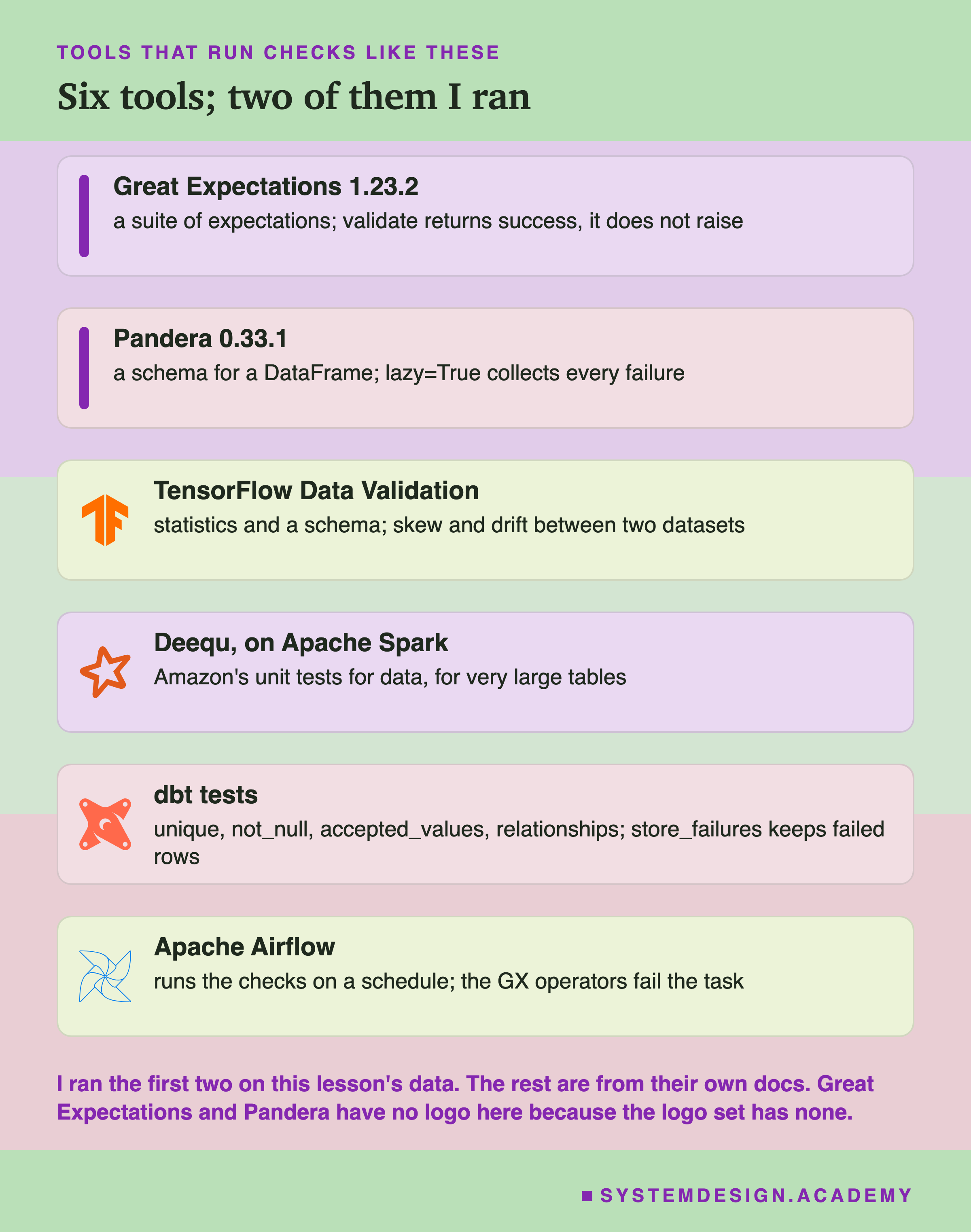
Six cards headed tools that run checks like these, titled six tools; two of them I ran. Great Expectations 1.23.2: a suite of expectations; validate returns success, it does not raise. Pandera 0.33.1: a schema for a DataFrame; lazy=True collects every failure. TensorFlow Data Validation, with the TensorFlow logo: statistics and a schema; skew and drift between two datasets. Deequ, on Apache Spark, with the Spark logo: Amazon's unit tests for data, for very large tables. dbt tests, with the dbt logo: unique, not_null, accepted_values, relationships; store_failures keeps failed rows. Apache Airflow, with its logo: runs the checks on a schedule; the GX operators fail the task. Beneath: I ran the first two on this lesson's data; the rest are from their own docs; Great Expectations and Pandera have no logo here because the logo set has none.

Great Expectations keeps checks in a suite, a named list of expectations. You run the suite on a batch and get back a result for each one. In version 1.x each expectation is a class, such as ExpectColumnValuesToBeBetween. One setting matters a lot for this lesson: mostly. Its documentation says an expectation is "successful if at least mostly fraction of values match". The default is 1, every row. I tried it on one real day from the lab, with three hours of temperature set to -999. With the default, the range check failed. With mostly=0.85 it passed, because 21 of 24 rows is more than 85%.

Pandera describes a pandas table as a schema: each column, its type, and its checks. With lazy=True it collects every failure before it stops, into a table called failure_cases. Pandera can also write a first schema from data, with infer_schema. Its docs warn that "these inferred schemas are rough drafts that shouldn't be used for validation without modification". That warning matters here, as you will see.

What the Lab Ran

I wrote the lab's design into the docstring of its script, validation_demo.py, on 30 September 2026, before it ever ran. The script is the same file you can copy from this lesson and run yourself.
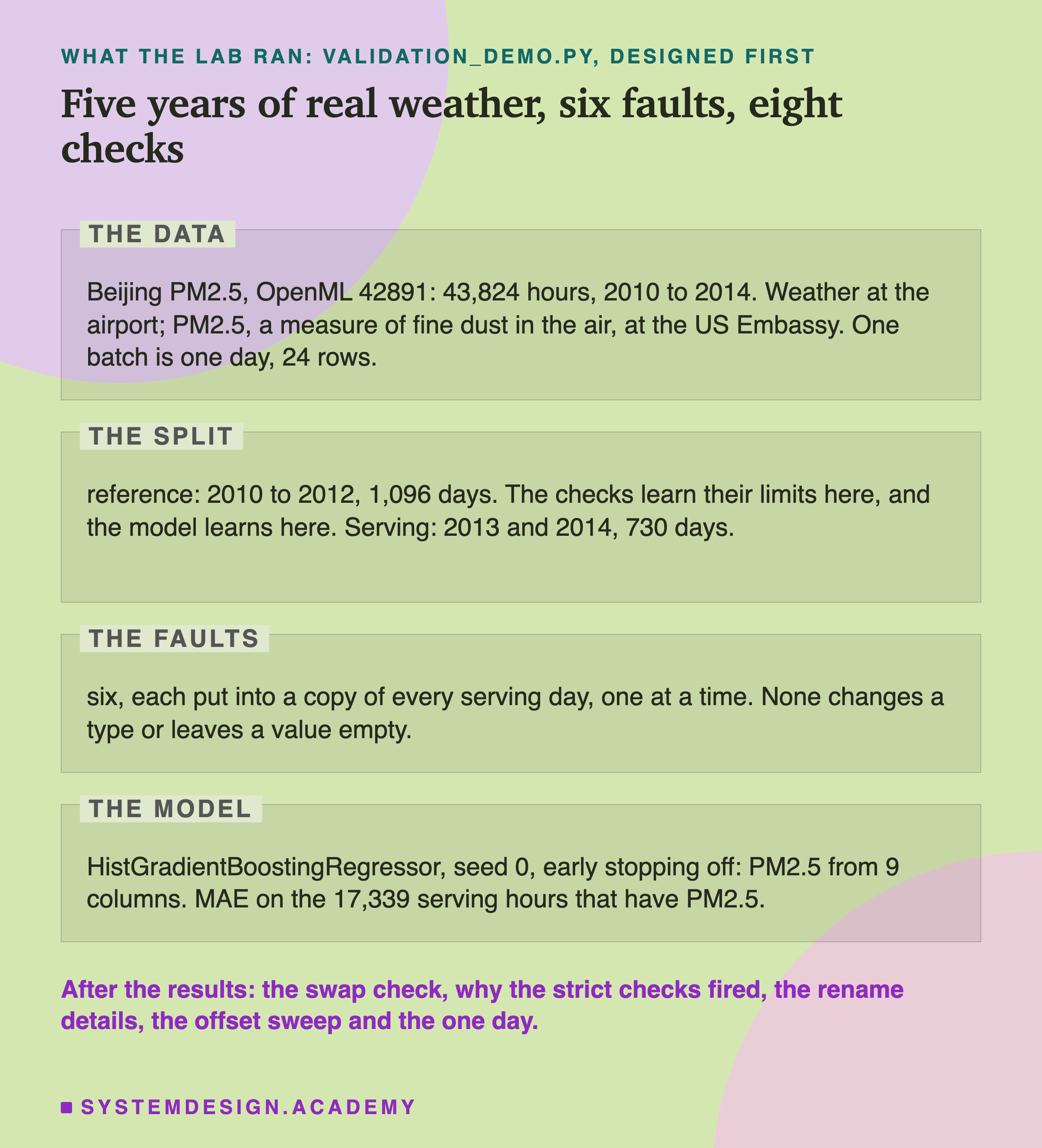
An editorial page in four labelled zones, headed what the lab ran: validation_demo.py, designed first, titled five years of real weather, six faults, eight checks. The data: Beijing PM2.5, OpenML 42891: 43,824 hours, 2010 to 2014; weather at the airport; PM2.5, a measure of fine dust in the air, at the US Embassy; one batch is one day, 24 rows. The split: reference, 2010 to 2012, 1,096 days; the checks learn their limits here, and the model learns here; serving, 2013 and 2014, 730 days. The faults: six, each put into a copy of every serving day, one at a time; none changes a type or leaves a value empty. The model: HistGradientBoostingRegressor, seed 0, early stopping off: PM2.5 from 9 columns; MAE on the 17,339 serving hours that have PM2.5. Beneath: after the results, the swap check, why the strict checks fired, the rename details, the offset sweep and the one day.

The data is the Beijing PM2.5 dataset, public on OpenML and in the UCI archive. It holds 43,824 hours from 2010 to 2014. Each hour has the weather at Beijing's airport and the PM2.5 reading at the US Embassy. PM2.5 is the amount of very fine dust in the air, in micrograms per cubic metre. The weather columns are dew point (DEWP) and temperature (TEMP), both in degrees C. There is also air pressure (PRES) in hectopascals (hPa), and a wind direction code (cbwd).

The split. The first three years, 1,096 days, are the reference. The checks take their limits from them, and the model learns from them. The last two years, 730 days, are serving: new data arriving one day at a time, as a daily file from a weather feed would.

The faults. I made six kinds of silent fault. For each one, I took a copy of every serving day and put that fault into it, one fault at a time. None of them changes a column's type or leaves a value empty, so none would trip lesson 2's table checks.

The model is scikit-learn's HistGradientBoostingRegressor: many small decision trees, built one after another. It predicts PM2.5 from nine columns: the hour, the month, the three sensors and the wind code. The last three are running totals of wind speed, hours of snow and hours of rain. I turned early stopping off. Lesson 2 found that it holds back a random tenth of the rows, so results moved with the random seed. One run.

False Alarms on Clean Days

The first question is the one I most often see skipped. On the 730 clean serving days, with no fault at all, how often did each check fire?
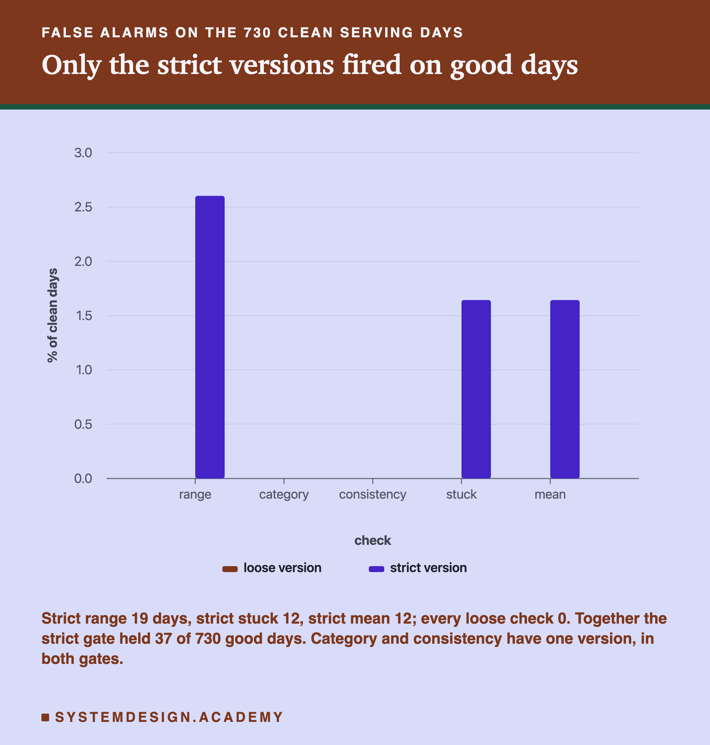
A bar chart headed false alarms on the 730 clean serving days, titled only the strict versions fired on good days. Five groups on the horizontal axis, range, category, consistency, stuck and mean, on a scale from 0 to 3 labelled percent of clean days, with a legend for a loose version and a strict version. Only three bars show: strict range near 2.6, and strict stuck and strict mean near 1.6. Every loose version is at 0, and category and consistency, which have one version each, are at 0. Beneath: strict range 19 days, strict stuck 12, strict mean 12; every loose check 0; together the strict gate held 37 of 730 good days; category and consistency have one version, in both gates.

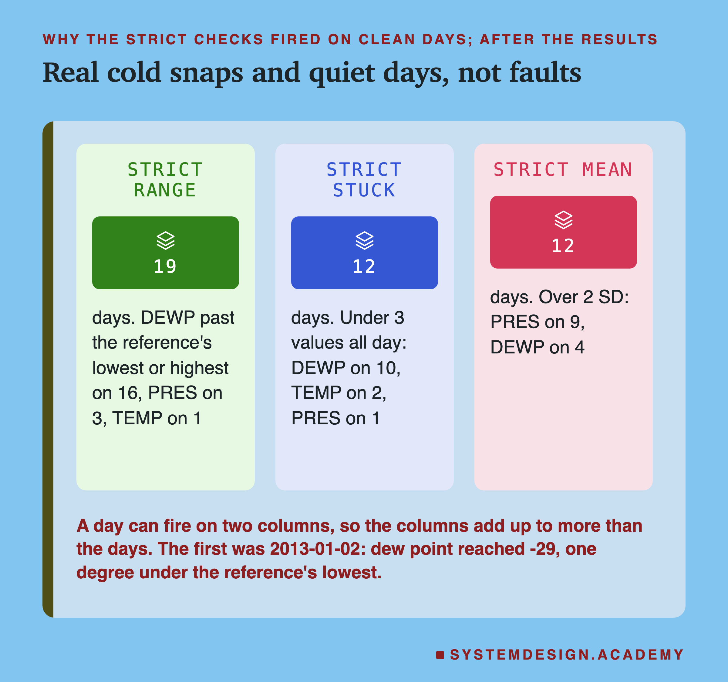
Every loose check stayed quiet on all 730 days. The strict ones did not. The strict range check fired on 19 days, the strict stuck check on 12, and the strict mean check on 12. Together, the strict gate would have held 37 good days, 5.1% of them. That is about one day in twenty, with nothing wrong.

Look at how the row rate and the day rate relate. The strict range check failed 117 of the 17,520 clean serving rows, 0.7%, and one failing row is enough to hold the whole day. If those 117 rows had been scattered at random, about 14.9% of days would have fired. That is 1 minus (1 minus 117 / 17,520) to the power 24. The check fired on 2.6%. I added that arithmetic to the report after a review.

The difference is that the failing rows came in groups, about 6 on each day that fired. That makes sense for weather: a cold, dry spell lasts hours, not one hour. So you cannot guess a check's day rate from its row rate alone. The safe way is to run it on clean history and count.

Google's data validation team found the same kind of problem at a much larger scale. Their 2019 paper, by Breck and others, tried a standard statistical test on 100 million points, with 0.01% of them replaced. A person would call the two samples the same. The test, they wrote, "would needlessly fire an alert 7 out of 10 times and would most likely be considered a flaky detection method".
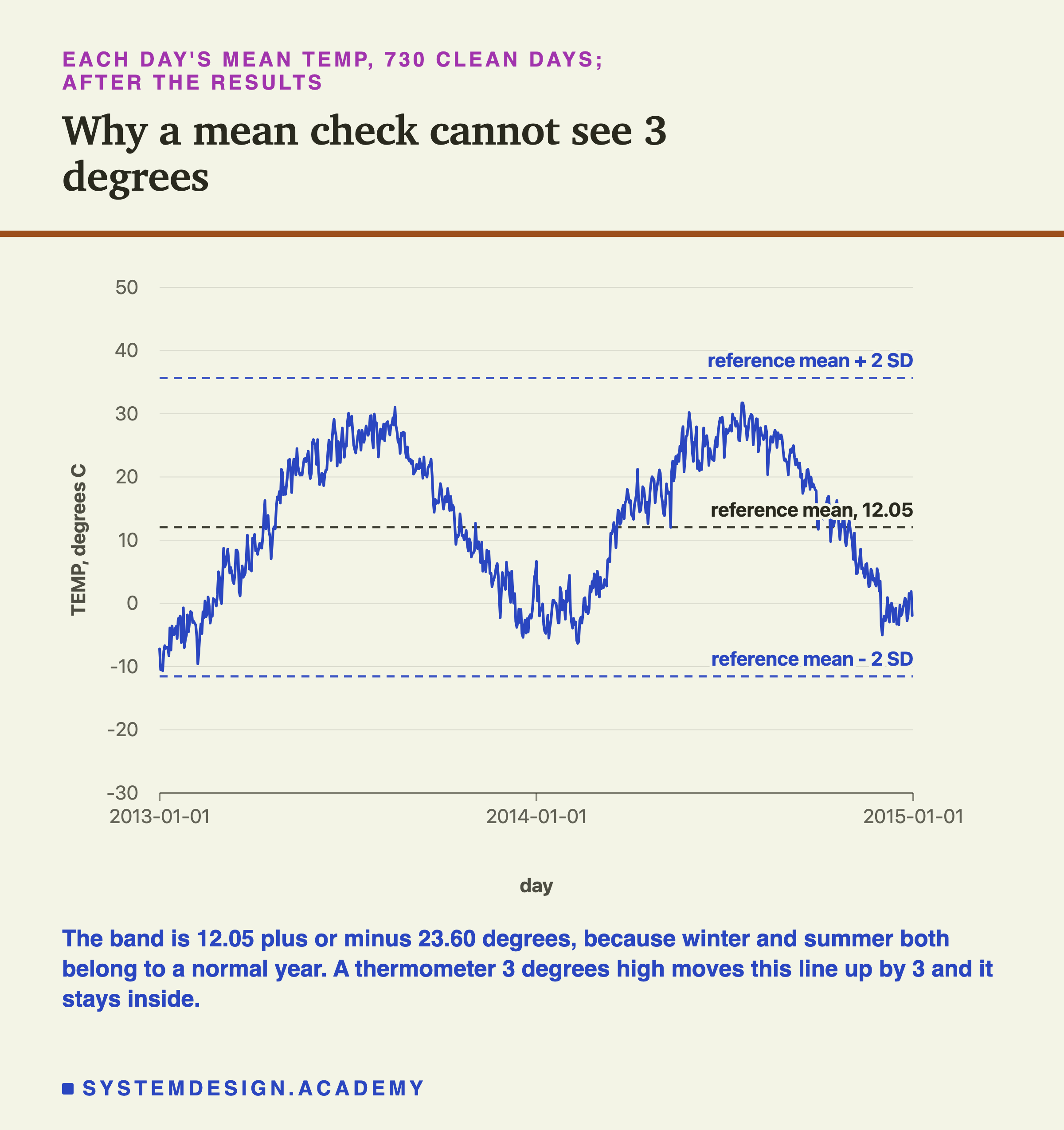
A line chart headed each day's mean TEMP, 730 clean days, after the results, titled why a mean check cannot see 3 degrees. The horizontal axis runs from 2013-01-01 through 2014-01-01 to 2015-01-01; the vertical axis is TEMP in degrees C from -30 to 50. One line rises from about -8 in January to about 30 in summer, falls to about -5 the next winter, and rises again. Three dashed lines: reference mean + 2 SD near 36, reference mean, 12.05, and reference mean - 2 SD near -12. The line stays between the outer two. Beneath: the band is 12.05 plus or minus 23.60 degrees, because winter and summer both belong to a normal year; a thermometer 3 degrees high moves this line up by 3 and it stays inside.

Which Check Caught Which Fault

Now the faults. For each one, I counted the days on which each check fired, out of the 730 faulty copies.
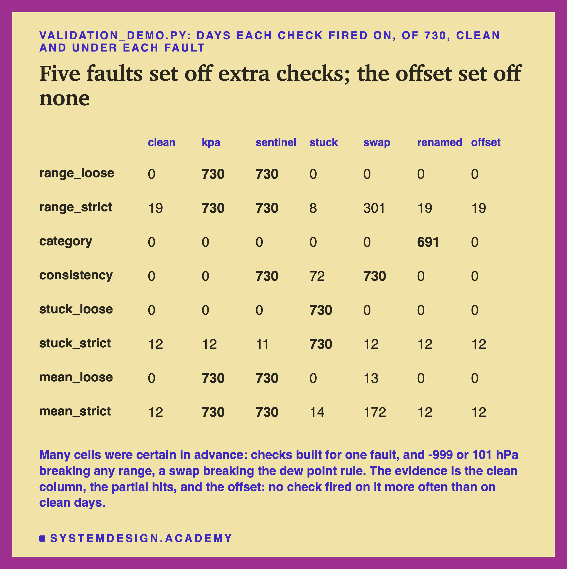
A table headed validation_demo.py: days each check fired on, of 730, clean and under each fault, titled five faults set off extra checks; the offset set off none. Columns clean, kpa, sentinel, stuck, swap, renamed, offset. range_loose: 0, 730, 730, 0, 0, 0, 0. range_strict: 19, 730, 730, 8, 301, 19, 19. category: 0, 0, 0, 0, 0, 691, 0. consistency: 0, 0, 730, 72, 730, 0, 0. stuck_loose: 0, 0, 0, 730, 0, 0, 0. stuck_strict: 12, 12, 11, 730, 12, 12, 12. mean_loose: 0, 730, 730, 0, 13, 0, 0. mean_strict: 12, 730, 730, 14, 172, 12, 12. Beneath: many cells were certain in advance: checks built for one fault, and -999 or 101 hPa breaking any range, a swap breaking the dew point rule; the evidence is the clean column, the partial hits, and the offset: no check fired on it more often than on clean days.

Be careful how you read this table. I built several checks with one fault in mind: the stuck check for the stuck sensor, the category check for the renamed code. Many other cells were certain by arithmetic. A value of -999 or a pressure of 101 hPa lies outside any sensible range, so every range check had to catch them. A swap puts the dew point above the air temperature in every hour where the air was warmer, so the dew point rule had to catch it. Those full columns show the checks were written correctly, not that checks in general catch faults.

The useful cells are the ones the arithmetic did not settle in advance. The stuck sensor set off the dew point rule on 72 days, when the air cooled below the frozen dew point. The mean checks caught the pressure in kilopascals on every day, which the band made certain too, but they barely noticed the stuck sensor.

The swap is the interesting one. The loose range check never saw it, because both columns hold values that are possible temperatures. The strict range check caught it on 301 days, and the strict mean check on 172. The one rule between the two columns caught it on all 730 days.

The renamed code was caught on 691 days. The other 39 days had no calm-wind hour at all, so there was nothing to rename. And the offset column matches the clean column exactly. No check fired on the thermometer error more often than it fired on clean days.

What Each Fault Did to the Model

A check that fires is only half the story. The other half is what the fault costs if nothing stops it. So I scored the clean model on each faulty copy of the 730 serving days. The model's error on clean serving days was an MAE of 46.39 micrograms per cubic metre.
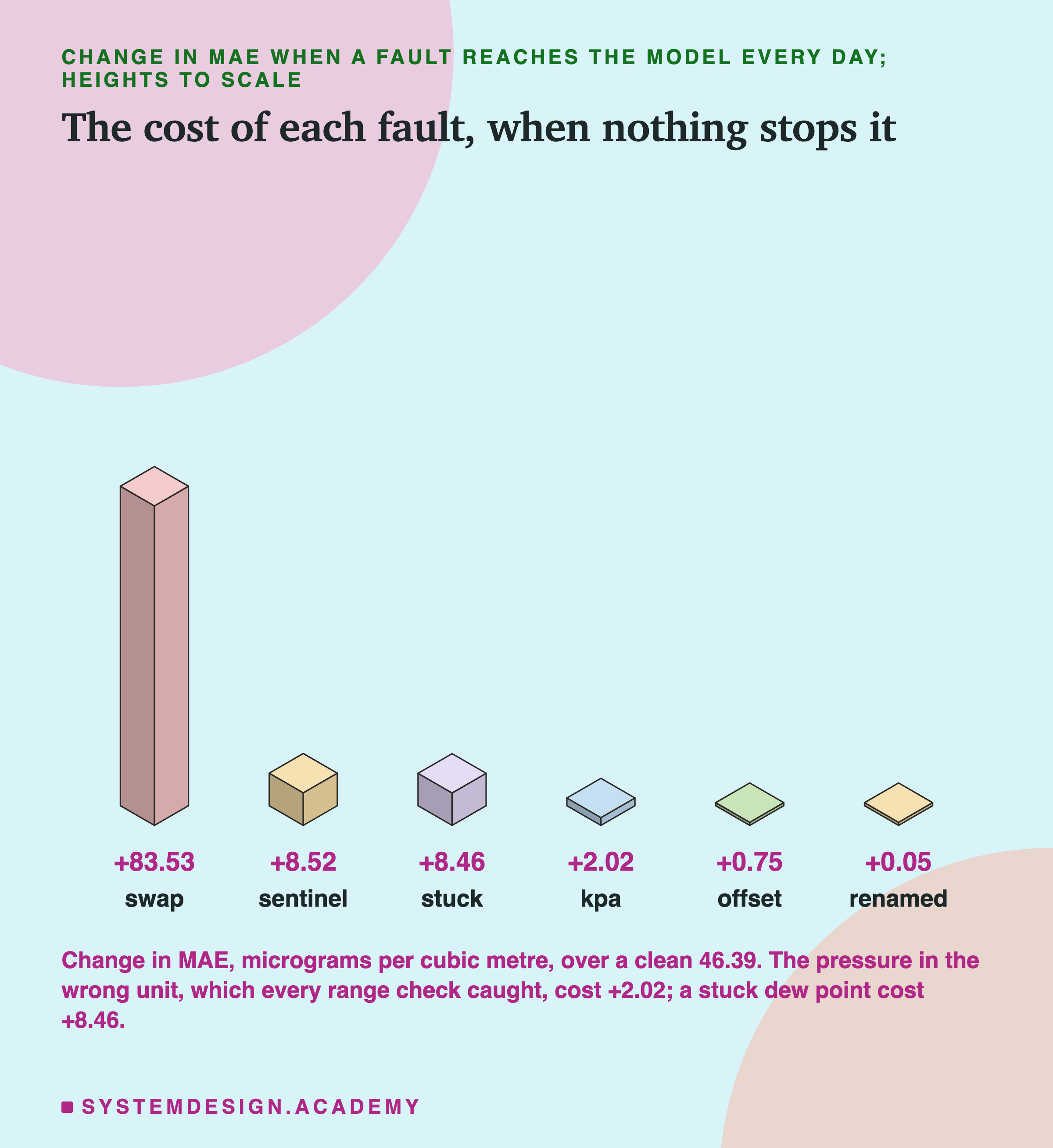
An isometric drawing of six blocks, heights to scale, headed change in MAE when a fault reaches the model every day, titled the cost of each fault, when nothing stops it. Swap, a tall block, +83.53. Sentinel, a low block, +8.52. Stuck, a low block, +8.46. Kpa, almost a tile, +2.02. Offset, a tile, +0.75. Renamed, a tile, +0.05. Beneath: change in MAE, micrograms per cubic metre, over a clean 46.39; the pressure in the wrong unit, which every range check caught, cost +2.02; a stuck dew point cost +8.46.

The swap was by far the most costly. It raised the MAE from 46.39 to 129.92, almost three times as bad. The -999 hours and the stuck sensor each added about 8.5. The pressure in kilopascals, the fault every range check caught, added only 2.02.

That surprised me. One possible reason is how trees work: they split on "pressure below some value", and a pressure of 101 is simply below every split. So the model treats every hour as the lowest pressure it knows, and pressure is only one of nine inputs. I did not test that reason. The lesson is that how easy a fault is to catch is a different question from what it costs.
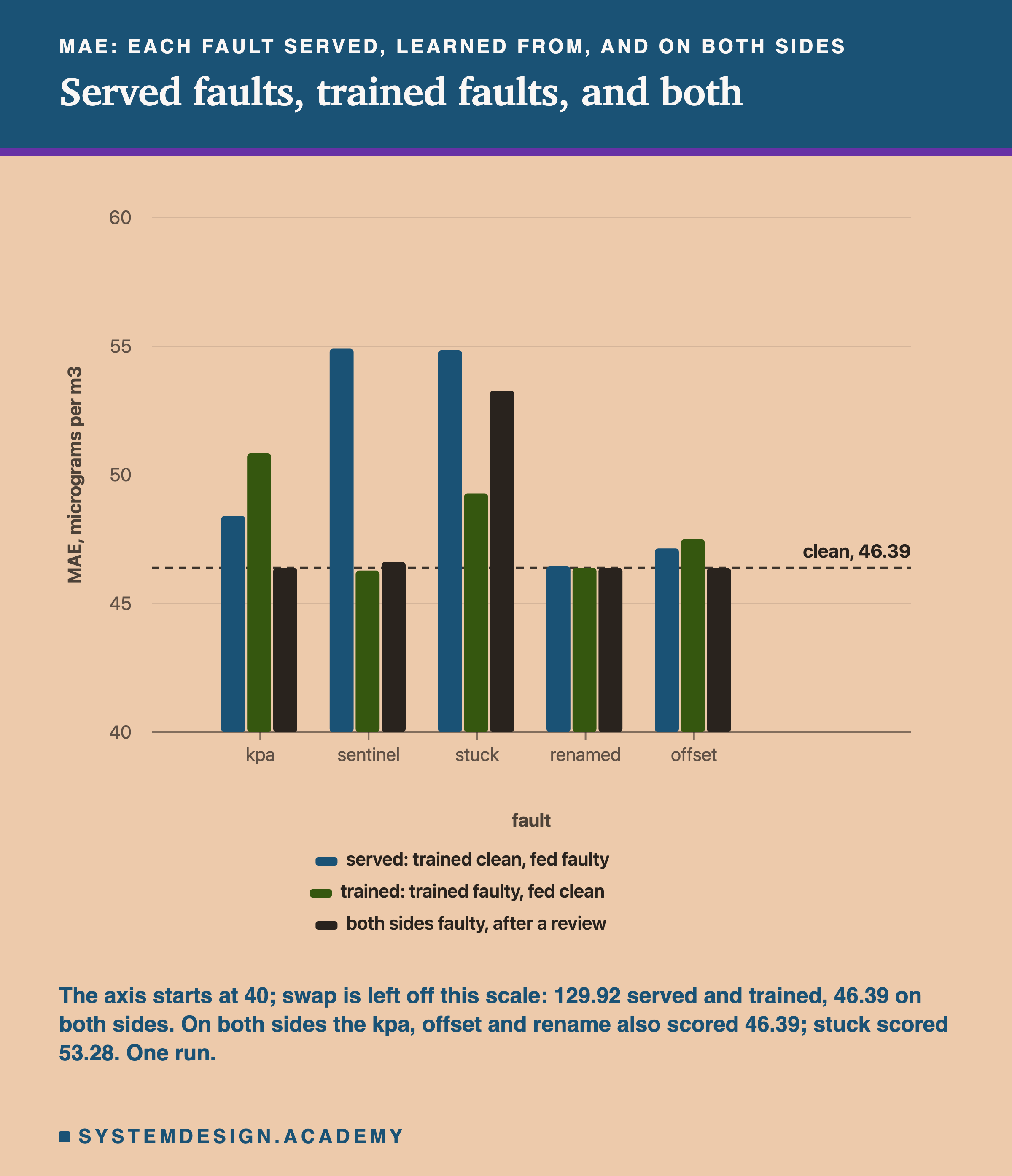
A bar chart headed MAE: each fault served, learned from, and on both sides, titled served faults, trained faults, and both. Five groups, kpa, sentinel, stuck, renamed and offset, each with three bars, on a scale from 40 to 60 labelled MAE, micrograms per m3, with a dashed line at clean, 46.39. Served, trained clean and fed faulty: near 48.4, 54.9, 54.9, 46.4 and 47.1. Trained, trained faulty and fed clean: near 50.8, 46.3, 49.3, 46.4 and 47.5. Both sides faulty, after a review: near 46.4, 46.6, 53.3, 46.4 and 46.4. Beneath: the axis starts at 40; swap is left off this scale: 129.92 served and trained, 46.39 on both sides; on both sides the kpa, offset and rename also scored 46.39; stuck scored 53.28; one run.

A fault can also reach a model through its training data. So I also trained a model on each faulty copy of the reference years, then fed it clean serving days. This chart shows both, with the swap left off because it would squash the scale. After a review, I added a third case to the report: the fault on both sides, in training and in serving.

The first two are the same kind of mistake seen from two sides. A served fault means a model trained on clean history is fed faulty data. A trained fault here means a model trained on faulty history is fed clean data. Both are a mismatch between what the model learned and what it is fed: training-serving skew. To a model that learned pressures near 101, a clean pressure of 1016 is far outside anything it saw.

The Fault No Check Saw

The offset is the fault this lesson is really about. The loose gate let a thermometer reading 3 degrees high through on all 730 days. The strict gate held 37 of them, but those were exactly the 37 days it holds with no fault at all. No check fired on the offset more often than on clean days. It cost the model 0.75 MAE on these two years, a gap the block bootstrap cannot tell apart from zero.

Why did no check react to it? Every value it produced was still possible. A 3 degree error sits well inside the range of a normal day and the spread of a normal year. It cannot break the dew point rule either, because it only makes the air warmer. It is the accuracy problem from the six questions: a value that is well-formed, and wrong.
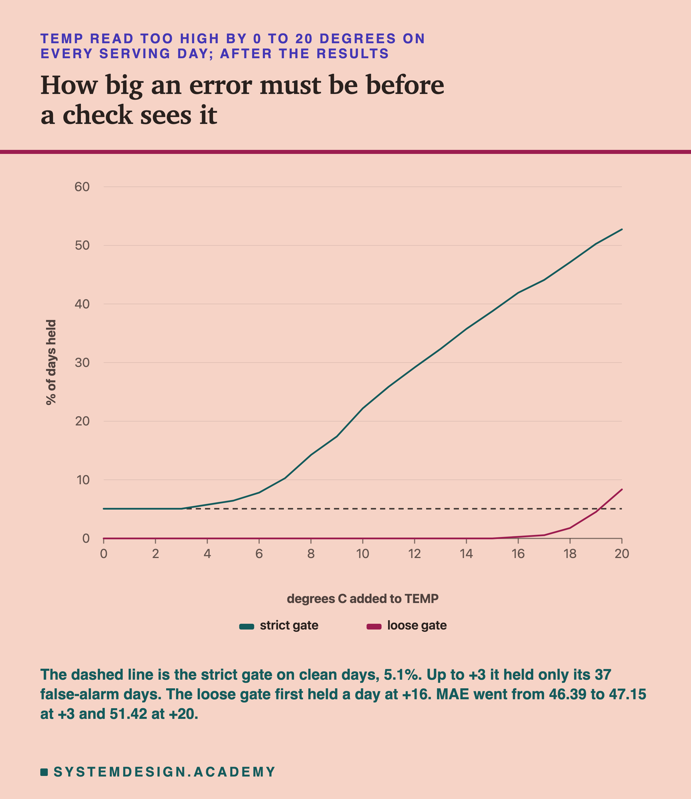
A line chart headed TEMP read too high by 0 to 20 degrees on every serving day, after the results, titled how big an error must be before a check sees it. The horizontal axis is degrees C added to TEMP, 0 to 20; the vertical axis is percent of days held, 0 to 60. The strict gate's line is flat near 5 up to +3, then rises slowly, passes 22 at +10 and reaches about 53 at +20. The loose gate's line sits at 0 until about +15, then rises to about 8 at +20. A dashed line runs across at the strict gate's clean level. Beneath: the dashed line is the strict gate on clean days, 5.1%; up to +3 it held only its 37 false-alarm days; the loose gate first held a day at +16; MAE went from 46.39 to 47.15 at +3 and 51.42 at +20.

After the results, I asked a follow-up question: how big must the error be before any check notices? I added 0 to 20 degrees to every serving day's temperature and ran the gates again.

Up to +3, the strict gate held exactly its 37 false-alarm days and nothing more. From +4 it started to hold extra days, slowly: 22.2% of days at +10, still with most days passing. The loose gate stayed quiet until +16. Meanwhile the model's error climbed the whole way, to 51.42 at +20.

What would a second source look like here? Suppose there were a second weather station nearby. A job could compare this airport's hourly temperature with that station's, and watch the difference between them. The two will never agree exactly, so the check is on the difference over weeks, not on one hour. A difference that moves by 3 degrees and stays there is the offset, found. I did not build this, because the dataset holds one station.

So the checks and the harm move on different scales. A small error costs the model something from the first degree, and the checks see nothing until the error is large. A tighter band would only add false alarms. What would help is a second source: a nearby weather station, a second sensor, or a person checking a sample now and then.

A Renamed Category

The renamed wind code shows a different kind of silence. The category check caught it on 691 of the 730 days. But when a check does not run, what does the pipeline itself do with a value it has never seen?
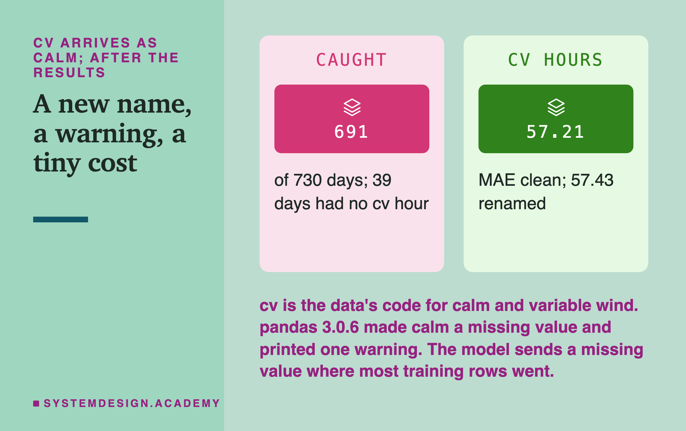
Two panels headed cv arrives as calm, after the results, titled a new name, a warning, a tiny cost. Caught: 691; of 730 days; 39 days had no cv hour. Cv hours: 57.21; MAE clean; 57.43 renamed. Beneath: cv is the data's code for calm and variable wind; pandas 3.0.6 made calm a missing value and printed one warning; the model sends a missing value where most training rows went.

The lab's feature job turns the wind code into a pandas category with a fixed list of codes. The pandas docs say "values not in categories will be replaced with NaN", a missing value. pandas 3.0.6 also prints a deprecation warning, saying a future version will raise an error. The job did not stop. The demo counts that warning, in a line I added after the first run: it came twice, once for each run that met the new code.

Then the model met a missing wind code. scikit-learn's guide says that when a feature had no missing values in training, "samples with missing values are mapped to whichever child has the most samples". So at each split on the wind code, those hours went down the busier branch.

The cost was tiny on this model. Calm wind came in 4,006 of the 17,520 serving hours, 22.9%. On those hours the MAE went from 57.21 to 57.43. One possible reason is that the model has another wind column to lean on, the running total of wind speed. A different model, or a dashboard counting calm hours, could be hurt far more. The check fired even though this model barely cared, and that is fine: a check protects every reader, not just one model.

Two Gates, and What to Do When One Fires

Put the checks together into the two gates, and the trade shows up clearly.
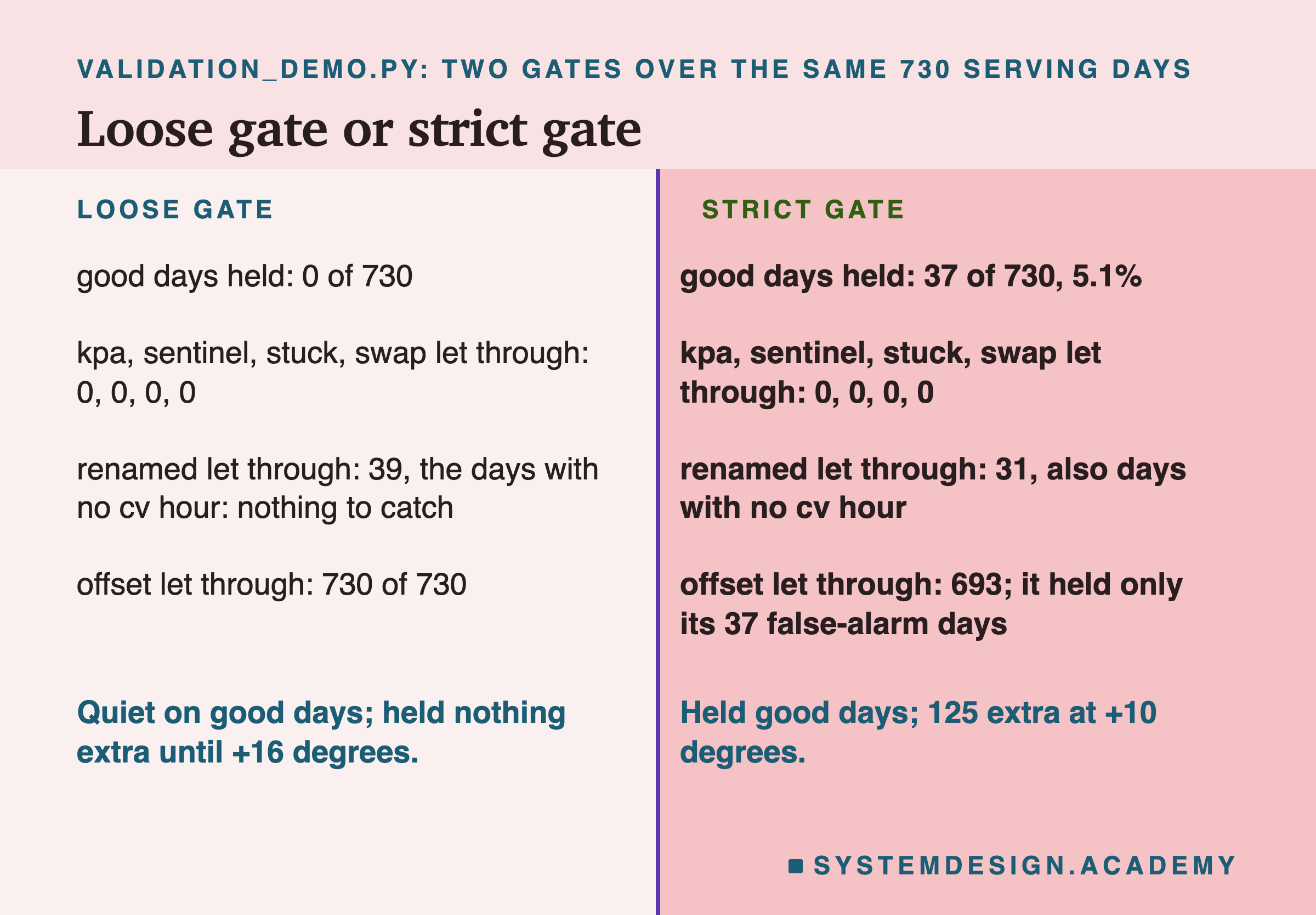
A two-column table headed validation_demo.py: two gates over the same 730 serving days, titled loose gate or strict gate. Left, loose gate: good days held: 0 of 730; kpa, sentinel, stuck, swap let through: 0, 0, 0, 0; renamed let through: 39, the days with no cv hour: nothing to catch; offset let through: 730 of 730. Right, strict gate: good days held: 37 of 730, 5.1%; kpa, sentinel, stuck, swap let through: 0, 0, 0, 0; renamed let through: 31, also days with no cv hour; offset let through: 693; it held only its 37 false-alarm days. Beneath: quiet on good days; held nothing extra until +16 degrees; held good days; 125 extra at +10 degrees.

Both gates caught every day of four faults: the kilopascals, the -999 hours, the stuck sensor and the swap. Both let through the renamed days that had no calm-wind hour, which was right, because nothing on those days had changed. I checked that in the report, day by day. Several of those catches were certain by arithmetic, as the table showed.

On these six faults, every faulty day the strict gate held and the loose gate let through was one of the strict gate's own 37 false-alarm days. The report checks that day by day. With the offset it held those same 37 days, and let the other 693 through. So is the loose gate simply better? Not quite. The offset sweep shows what the strict gate buys. At +10 degrees it held 22.2% of days, 125 more than on clean days, while the loose gate held nothing until +16. The strict gate costs good days and buys earlier warning of a large error.

A gate also needs a rule for what happens when it fires. Decide it before the failure, so nobody has to make it up at 3 in the morning.
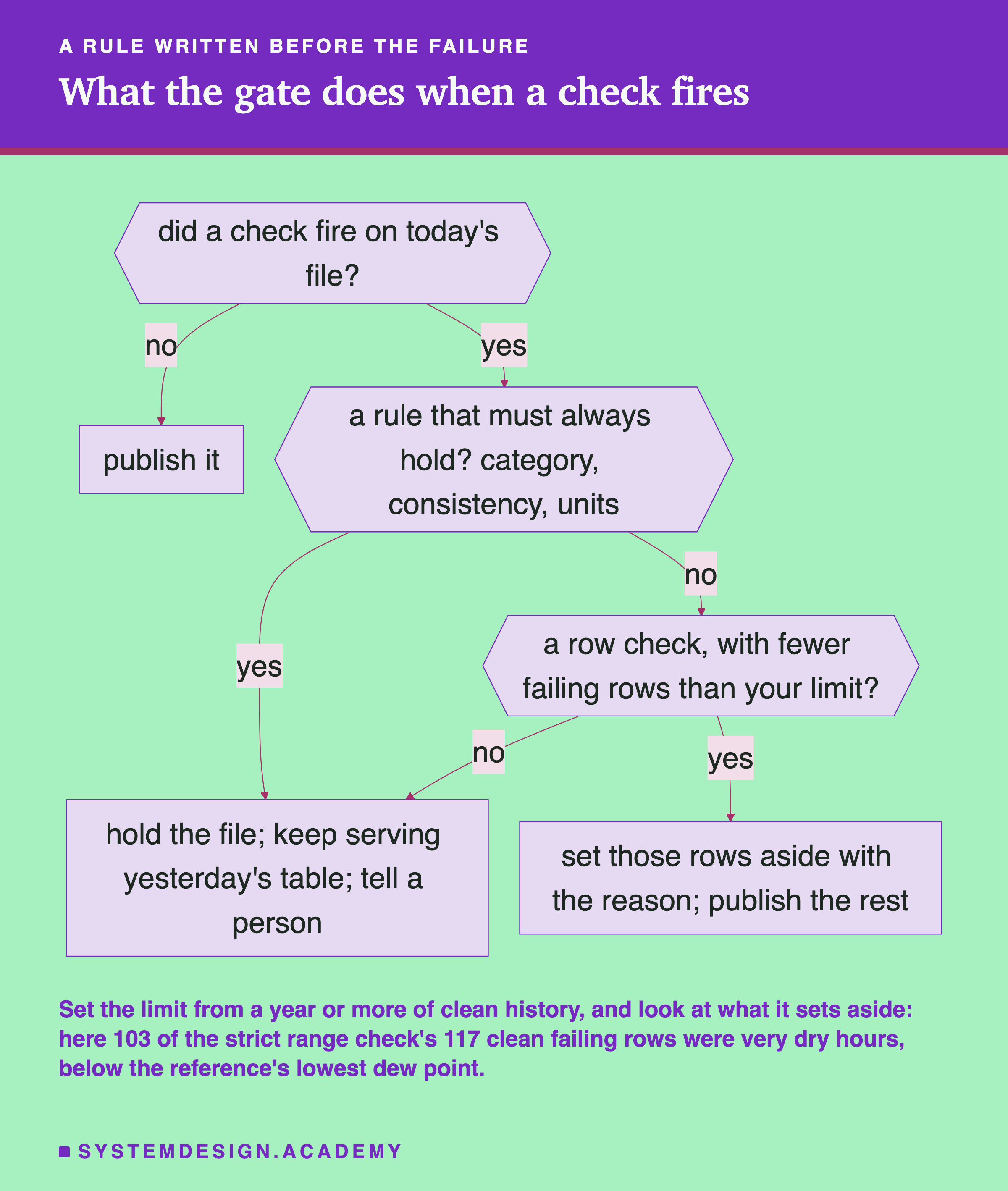
A flowchart headed a rule written before the failure, titled what the gate does when a check fires. A diamond, did a check fire on today's file? No leads to publish it. Yes leads to a diamond, a rule that must always hold? category, consistency, units. Yes leads to hold the file; keep serving yesterday's table; tell a person. No leads to a diamond, a row check, with fewer failing rows than your limit? Yes leads to set those rows aside with the reason; publish the rest. No leads back to hold the file. Beneath: set the limit from a year or more of clean history, and look at what it sets aside: here 103 of the strict range check's 117 clean failing rows were very dry hours, below the reference's lowest dew point.

Some rules must always hold: a known unit, a known category, dew point not above air temperature. When one of those fails, hold the whole file. The table keeps serving yesterday's data while a person looks. My view is that a model on day-old data is usually safer than a model on wrong data, though this lab did not measure that.

Profiles, Drift and Skew

Most checks in this lesson look at one value at a time. The mean checks are different. They look at a profile: numbers that describe a whole batch, such as its average, its spread, or how often each category appears. A profile check can see a batch whose values are each possible but whose shape has moved.

That shape is called a distribution: how the values of a column are spread out, how many are low and how many high. When it moves over time, that is drift. When the data a model learned from and the data it now serves differ at the same moment, that is training-serving skew.

Common Mistakes, and When Not to Add a Check

These are the mistakes I would look for first when I review a validation setup. They are general practice, not measurements, except where I say the lab measured something.

A gate that only warns. If a failed check writes a log line and the job carries on, you have a report, not a gate. Great Expectations returns success as False and raises nothing. Something in your pipeline has to act on it. Feed the gate a broken batch on purpose, and watch it stop.

Validating after the write. If the data lands in the shared table first, readers can see bad rows before any check runs. Stage it, check it, then publish it.

Limits taken from the data's own minimum and maximum. That is what infer_schema writes, and its docs call the result a rough draft. Here it fired on 19 good days in two years.

A baseline that follows the drift. If you rebuild the profile from last week every week, a slow drift moves the baseline with it, and the alarm never fires. Freeze it from data you trust, and change it on purpose when you retrain.

Only per-row checks. A batch can pass every row rule and still be wrong in shape. Add a profile check on the columns a model reads.

Dropping failed rows. A dropped row cannot be replayed or explained later.

When not to add a check. Not every column needs a rule. A free-text note that no model reads does not need a range. Every check costs run time and attention, and a check that fires often trains people to ignore it.

How Real Teams Describe It

The old version of this lesson told four company stories. I checked each one against the company's own words, and none held up as written. Uber was said to have one feature feeding "hundreds of models", Netflix to protect "millions of users", and Airbnb to have acted because "trust in a metric collapses". I could not find any of those claims in the companies' own posts, so I have cut them.

Here is what five teams do say, in their own posts and papers.
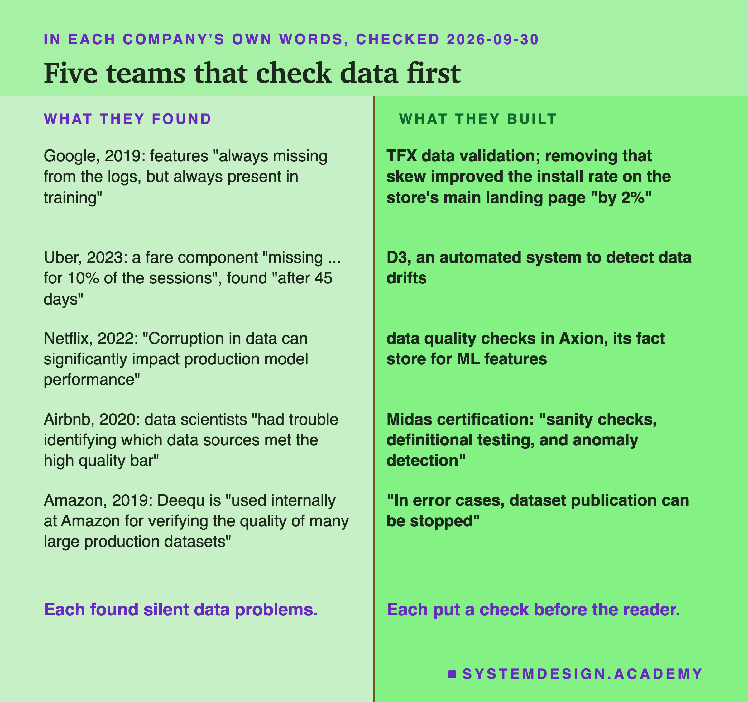
A two-column table headed in each company's own words, checked 2026-09-30, titled five teams that check data first. Left, what they found; right, what they built. Google, 2019: features always missing from the logs, but always present in training; TFX data validation; removing that skew improved the install rate on the store's main landing page by 2%. Uber, 2023: a fare component missing for 10% of the sessions, found after 45 days; D3, an automated system to detect data drifts. Netflix, 2022: corruption in data can significantly impact production model performance; data quality checks in Axion, its fact store for ML features. Airbnb, 2020: data scientists had trouble identifying which data sources met the high quality bar; Midas certification: sanity checks, definitional testing, and anomaly detection. Amazon, 2019: Deequ is used internally at Amazon for verifying the quality of many large production datasets; in error cases, dataset publication can be stopped. Beneath: each found silent data problems; each put a check before the reader.

Google. Breck and others wrote in 2019 that "hundreds of product teams use our system to validate trillions of training and serving examples per day". Their Play store case is on the previous slide.

Uber. In February 2023 Uber wrote that "data regressions are hard to catch because the most impactful ones are generally silent". In one incident, a fare component "was missing in the critical fares dataset for 10% of the sessions". It "was detected after 45 days manually by one of the data scientists". Uber built D3 to detect such drifts automatically. Its post names the same trade as this lab: "Base limits can sometimes be more aggressive and generate many false positives". So, it says, "we define conservative alerting limits on top of the base ones".

Netflix. Netflix wrote about Axion in 2022. In its words, Axion is "our fact store that is leveraged to compute ML features offline". The post says: "Corruption in data can significantly impact production model performance and A/B test results".

Airbnb. A 2019 survey found its data scientists "had trouble identifying which data sources met the high quality bar required for their work". For its Midas certification, checks "are required for certified data, and cover basic sanity checks, definitional testing, and anomaly detection".

Try It Yourself

This script is the lab. It downloads the weather data, puts in the six faults, and runs the eight checks on clean and faulty days. It builds the two gates and trains the models. It prints the false alarms, the catches, the gates and the MAE for every fault. It needs no GPU; when I ran it, it finished in about 5 seconds once the data was downloaded.
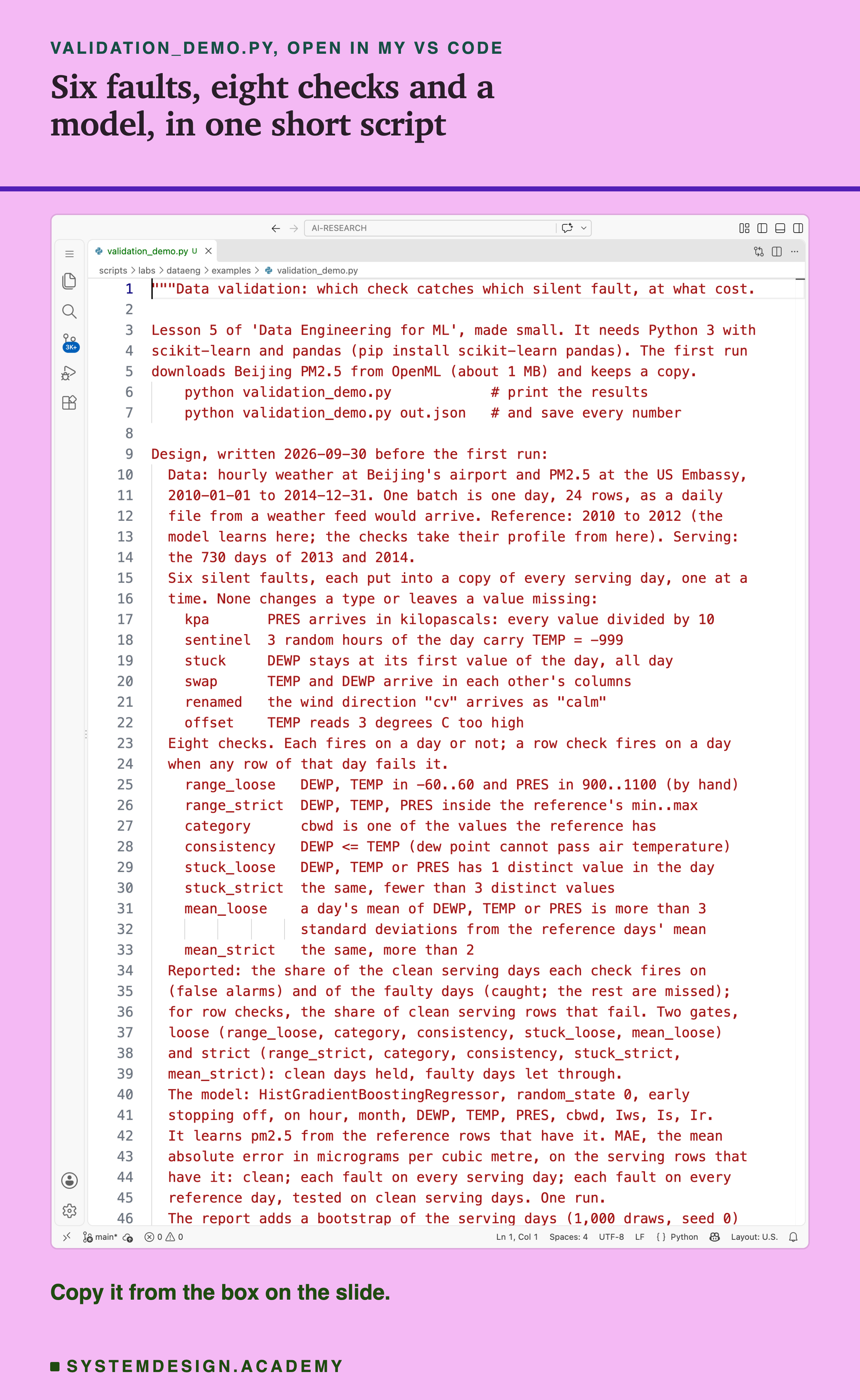
A real screenshot of VS Code with validation_demo.py open at the top of the file: the docstring, which says the script needs Python 3 with scikit-learn and pandas and how to run it, and holds the design written on 2026-09-30 before the first run: the data, hourly weather at Beijing's airport and PM2.5 at the US Embassy from 2010 to 2014, one batch a day; the reference years 2010 to 2012 and the 730 serving days; the six silent faults, kpa, sentinel, stuck, swap, renamed and offset; the eight checks with their limits; what is reported, and the two gates; and the model, HistGradientBoostingRegressor with early stopping off, scored by MAE. The rest of the docstring, the imports and the code are further down. Beneath: copy it from the box on the slide.

Before you run this lab. You need Python 3 and two libraries: pip install scikit-learn pandas. scikit-learn holds the model and the download, and brings NumPy with it; pandas holds the tables. The first run downloads Beijing PM2.5 from OpenML, about 1 MB, so it needs an internet connection once. After that, scikit-learn keeps a copy in a folder in your home directory (scikit_learn_data).

I ran it with scikit-learn 1.9.1 and pandas 3.0.6 on a Mac. Both run the same way on Windows and Linux, but I have not checked the numbers there. Another version may give different decimals, so the first line printed names both versions. Give it a file name, python validation_demo.py out.json, and it also saves every number at full precision; that is how results/dq-demo.json was made.

"""Data validation: which check catches which silent fault, at what cost.

Lesson 5 of 'Data Engineering for ML', made small. It needs Python 3 with
scikit-learn and pandas (pip install scikit-learn pandas). The first run
downloads Beijing PM2.5 from OpenML (about 1 MB) and keeps a copy.
    python validation_demo.py            # print the results
    python validation_demo.py out.json   # and save every number

Design, written 2026-09-30 before the first run:
  Data: hourly weather at Beijing's airport and PM2.5 at the US Embassy,
  2010-01-01 to 2014-12-31. One batch is one day, 24 rows, as a daily
  file from a weather feed would arrive. Reference: 2010 to 2012 (the
  model learns here; the checks take their profile from here). Serving:
  the 730 days of 2013 and 2014.
  Six silent faults, each put into a copy of every serving day, one at a
  time. None changes a type or leaves a value missing:
    kpa       PRES arrives in kilopascals: every value divided by 10
    sentinel  3 random hours of the day carry TEMP = -999
    stuck     DEWP stays at its first value of the day, all day
    swap      TEMP and DEWP arrive in each other's columns
    renamed   the wind direction "cv" arrives as "calm"
    offset    TEMP reads 3 degrees C too high
  Eight checks. Each fires on a day or not; a row check fires on a day
  when any row of that day fails it.
    range_loose   DEWP, TEMP in -60..60 and PRES in 900..1100 (by hand)
    range_strict  DEWP, TEMP, PRES inside the reference's min..max
    category      cbwd is one of the values the reference has
    consistency   DEWP <= TEMP (dew point cannot pass air temperature)
    stuck_loose   DEWP, TEMP or PRES has 1 distinct value in the day
    stuck_strict  the same, fewer than 3 distinct values
    mean_loose    a day's mean of DEWP, TEMP or PRES is more than 3
                  standard deviations from the reference days' mean
    mean_strict   the same, more than 2
  Reported: the share of the clean serving days each check fires on
  (false alarms) and of the faulty days (caught; the rest are missed);
  for row checks, the share of clean serving rows that fail. Two gates,
  loose (range_loose, category, consistency, stuck_loose, mean_loose)
  and strict (range_strict, category, consistency, stuck_strict,
  mean_strict): clean days held, faulty days let through.
  The model: HistGradientBoostingRegressor, random_state 0, early
  stopping off, on hour, month, DEWP, TEMP, PRES, cbwd, Iws, Is, Ir.
  It learns pm2.5 from the reference rows that have it. MAE, the mean
  absolute error in micrograms per cubic metre, on the serving rows that
  have it: clean; each fault on every serving day; each fault on every
  reference day, tested on clean serving days. One run.
  The report adds a bootstrap of the serving days (1,000 draws, seed 0)
  for each serving fault's MAE gap, and a count of the raw data's own
  problems (missing pm2.5 by year, rows with DEWP above TEMP, repeated
  hours), and nothing else.
  After the first run, two changes, neither to a number: the first line
  printed also names the pandas version, and the warning pandas gives
  for the renamed wind code is counted and printed as one short line, so
  the printed run holds everything the terminal shows.

Author: Roni Das
Created: 2026-09-30
"""
import json
import sys
import warnings

import numpy as np
import pandas as pd
import sklearn
from sklearn.datasets import fetch_openml
from sklearn.ensemble import HistGradientBoostingRegressor

S = ["DEWP", "TEMP", "PRES"]  # the three sensor columns the checks watch
X_COLS = ["hour", "month", "DEWP", "TEMP", "PRES", "cbwd", "Iws", "Is", "Ir"]
LOOSE = {"DEWP": (-60, 60), "TEMP": (-60, 60), "PRES": (900, 1100)}
FAULTS = ["kpa", "sentinel", "stuck", "swap", "renamed", "offset"]
CHECKS = ["range_loose", "range_strict", "category", "consistency",
          "stuck_loose", "stuck_strict", "mean_loose", "mean_strict"]
GATES = {"loose": ["range_loose", "category", "consistency",
                   "stuck_loose", "mean_loose"],
         "strict": ["range_strict", "category", "consistency",
                    "stuck_strict", "mean_strict"]}

raw = fetch_openml(data_id=42891, as_frame=True, parser="auto").frame
raw["cbwd"] = raw["cbwd"].astype(str)
raw["day"] = pd.to_datetime(raw[["year", "month", "day"]])
ref, srv = raw[raw["year"] <= 2012], raw[raw["year"] >= 2013]

# The frozen profile: everything the checks know, taken from the reference.
CATS = sorted(ref["cbwd"].unique())
LO, HI = ref[S].min(), ref[S].max()
day_means = ref.groupby("day")[S].mean()
MU, SD = day_means.mean(), day_means.std()


def fault(d, kind):
    """A copy of the rows d with one silent fault in every day."""
    d = d.copy()
    if kind == "kpa":
        d["PRES"] = d["PRES"] / 10
    elif kind == "sentinel":  # the 3 hours with the smallest random key
        key = pd.Series(np.random.default_rng(0).random(len(d)), d.index)
        d.loc[key.groupby(d["day"]).rank(method="first") <= 3, "TEMP"] = -999
    elif kind == "stuck":
        d["DEWP"] = d.groupby("day")["DEWP"].transform("first")
    elif kind == "swap":
        d["TEMP"], d["DEWP"] = d["DEWP"].astype(float), d["TEMP"]
    elif kind == "renamed":
        d["cbwd"] = d["cbwd"].replace("cv", "calm")
    elif kind == "offset":
        d["TEMP"] = d["TEMP"] + 3
    return d


def run_checks(d):
    """Which checks fire on each day of d, and which rows fail."""
    rows = pd.DataFrame({
        "range_loose": ~pd.concat([d[c].between(*LOOSE[c]) for c in S],
                                  axis=1).all(axis=1),
        "range_strict": ~pd.concat([d[c].between(LO[c], HI[c]) for c in S],
                                   axis=1).all(axis=1),
        "category": ~d["cbwd"].isin(CATS),
        "consistency": d["DEWP"] > d["TEMP"],
    })
    days = rows.groupby(d["day"]).any()
    g = d.groupby("day")[S]
    distinct = g.nunique().min(axis=1)
    days["stuck_loose"], days["stuck_strict"] = distinct < 2, distinct < 3
    z = ((g.mean() - MU) / SD).abs().max(axis=1)
    days["mean_loose"], days["mean_strict"] = z > 3, z > 2
    return days[CHECKS], rows


WARNED = []  # what pandas warns about while the job builds its table


def table(d):
    """The feature job: the model's columns, cbwd as a fixed category."""
    X = d[X_COLS].copy()
    with warnings.catch_warnings(record=True) as caught_now:
        warnings.simplefilter("always")
        X["cbwd"] = pd.Categorical(X["cbwd"], categories=CATS)
    WARNED.extend(str(w.message) for w in caught_now)
    return X


def fit(d):
    d = d[d["pm2.5"].notna()]
    model = HistGradientBoostingRegressor(
        random_state=0, early_stopping=False, categorical_features="from_dtype")
    return model.fit(table(d), d["pm2.5"])


def mae(model, d):
    d = d[d["pm2.5"].notna()]
    return float((model.predict(table(d)) - d["pm2.5"]).abs().mean())


n_days = srv["day"].nunique()
out = {"scikit_learn": sklearn.__version__, "pandas": pd.__version__,
       "rows": len(raw),
       "ref_days": ref["day"].nunique(), "serving_days": n_days,
       "categories": CATS, "lo": LO.to_dict(), "hi": HI.to_dict(),
       "mu": MU.to_dict(), "sd": SD.to_dict()}
print(f"scikit-learn {sklearn.__version__}, pandas {pd.__version__}")
print(f"rows {len(raw):,}; days: reference {out['ref_days']:,}, "
      f"serving {n_days}")

clean_days, clean_rows = run_checks(srv)
out["false_alarm"] = clean_days.mean().to_dict()
out["clean_rows_failing"] = clean_rows.mean().to_dict()
print(f"false alarms, of {n_days} clean days:")
for c in CHECKS:
    print(f"  {c:<13} {clean_days[c].mean():6.1%}")

caught = {k: run_checks(fault(srv, k))[0] for k in FAULTS}
out["caught"] = {k: caught[k].mean().to_dict() for k in FAULTS}
out["caught_new"] = {k: (caught[k] & ~clean_days).mean().to_dict()
                     for k in FAULTS}
print(f"faulty days caught, % of {n_days}:")
print("  " + " " * 13 + "".join(f"{k[:5]:>6}" for k in FAULTS))
for c in CHECKS:
    print(f"  {c:<13}" + "".join(f"{caught[k][c].mean():6.0%}"
                                   for k in FAULTS))

out["gates"] = {}
print("gates: clean days held, faulty let through")
for gname, cs in GATES.items():
    held = clean_days[cs].any(axis=1).mean()
    through = {k: float(1 - caught[k][cs].any(axis=1).mean())
               for k in FAULTS}
    out["gates"][gname] = {"clean_held": float(held), "through": through}
    print(f"  {gname:<7}{held:5.1%} held;" + "".join(
        f" {through[k]:.0%}" for k in FAULTS))

model = fit(ref)
out["mae_clean"] = mae(model, srv)
out["mae_served"] = {k: mae(model, fault(srv, k)) for k in FAULTS}
out["mae_trained"] = {k: mae(fit(fault(ref, k)), srv) for k in FAULTS}
print(f"MAE, micrograms per m3; clean {out['mae_clean']:.1f}")
print(f"  {'fault':<9} {'served':>7} {'trained':>8}")
for k in FAULTS:
    print(f"  {k:<9} {out['mae_served'][k]:7.1f} "
          f"{out['mae_trained'][k]:8.1f}")

out["pandas_warnings"] = WARNED
print(f"pandas warnings: {len(WARNED)} (a category it does not know)")

if len(sys.argv) > 1:  # a file name was given: save every number too
    json.dump(out, open(sys.argv[1], "w"), indent=1)

The Lab Report
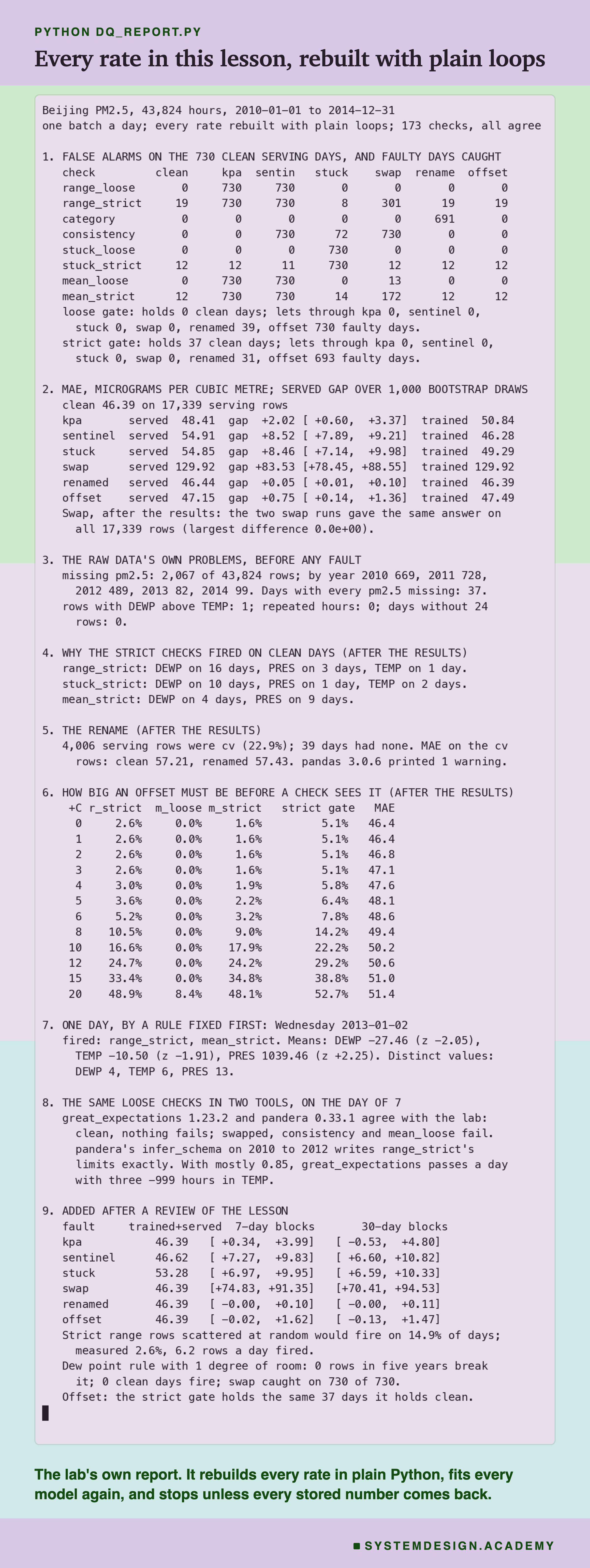
A real terminal recording headed python dq_report.py, titled every rate in this lesson, rebuilt with plain loops. It opens: Beijing PM2.5, 43,824 hours, 2010-01-01 to 2014-12-31; one batch a day; every rate rebuilt with plain loops; 173 checks, all agree. Then nine numbered sections: 1, the days each check fired on, clean and under each fault, and the two gates; 2, the MAE for each fault served and trained, with the served gap and its middle 95% over 1,000 bootstrap draws; 3, the raw data's own problems: 2,067 missing pm2.5, 1 row with DEWP above TEMP, 0 repeated hours; 4, why the strict checks fired on clean days; 5, the rename; 6, offsets from 0 to 20 degrees; 7, one day, Wednesday 2013-01-02; 8, the same loose checks in two tools, and mostly 0.85 passing a day with three -999 hours; 9, added after a review: the MAE with each fault on both sides, the served gaps over 7-day and 30-day blocks, the day rate if the strict range check's failing rows had been scattered at random, 14.9% against a measured 2.6%, the dew point rule with 1 degree of room, and the offset's 37 held days, the same as clean. Beneath: the lab's own report; it rebuilds every rate in plain Python, fits every model again, and stops unless every stored number comes back.

The report lives in scripts/labs/dataeng/dq_report.py. It reads the demo's stored files, results/dq-demo.json and the printed run, and the weather data from scikit-learn's local copy. It does not trust the demo's arithmetic. The demo puts in the faults and runs the checks with pandas. The report holds the 43,824 hours as plain Python dictionaries and does it all again with loops.

Then it fits every model again on tables it builds itself. It stops unless every stored rate comes back exactly and every MAE to within a billionth. It also reads the tool script's stored results. It stops unless both tools fail exactly the rules the lab's loose checks fail on that day. And it stops unless Pandera's inferred limits equal the strict range limits. All 173 checks agreed.

What came before the run is in the demo's docstring: the data, the split, the six faults, the eight checks, the two gates, the model and the bootstrap. What came after I saw the results is in the report's docstring, written before the report first ran. So is a later part, added after a review of this lesson. It covers the faults on both sides, the block bootstrap, the scattered-rows arithmetic and the 1-degree dew point rule. That covers the swap check, why the strict checks fired, the rename details, the offset sweep and the one day. Every figure that shows one of those says "after the results".

Run the Checks Yourself, No Model

This box has no model in it. It holds every hour of 2014, the second serving year: 8,760 hours of dew point, temperature, pressure and wind code. It also holds the limits the checks learned from 2010 to 2012, and the three hours of each day the lab's random draw gave the -999 fault. It puts in each fault, runs all eight checks, and builds the two gates, in your browser. Each number is stored as characters in base 64, which just means counting with 64 digits instead of 10, so the box stays small.

The report checked the box against the lab's own checks on 2014, count for count. Because it holds one year, not two, its counts are for 365 days. As it is, it prints that the strict range check fired on 10 clean days, the strict stuck check on 4 and the strict mean check on 3. The strict gate held 15 clean days, and the loose gate held none.

Then try your own limits. Change z > 2 in checks to z > 2.5, and count the false alarms again. Change row[1] + 3 in fault to row[1] + 10, and see which checks start to fire on the offset. Or change the loose TEMP limit in LOOSE from (-60, 60) to (-20, 45), and see what that range check now catches, and what it now holds by mistake.

Working One Day Out by Hand

Before you trust a check, I think you should be able to work it out with a pencil. So here is one real day. I picked it by a rule fixed before looking at any day: the earliest clean serving day on which a check of the strict gate fired. That was Wednesday 2 January 2013.
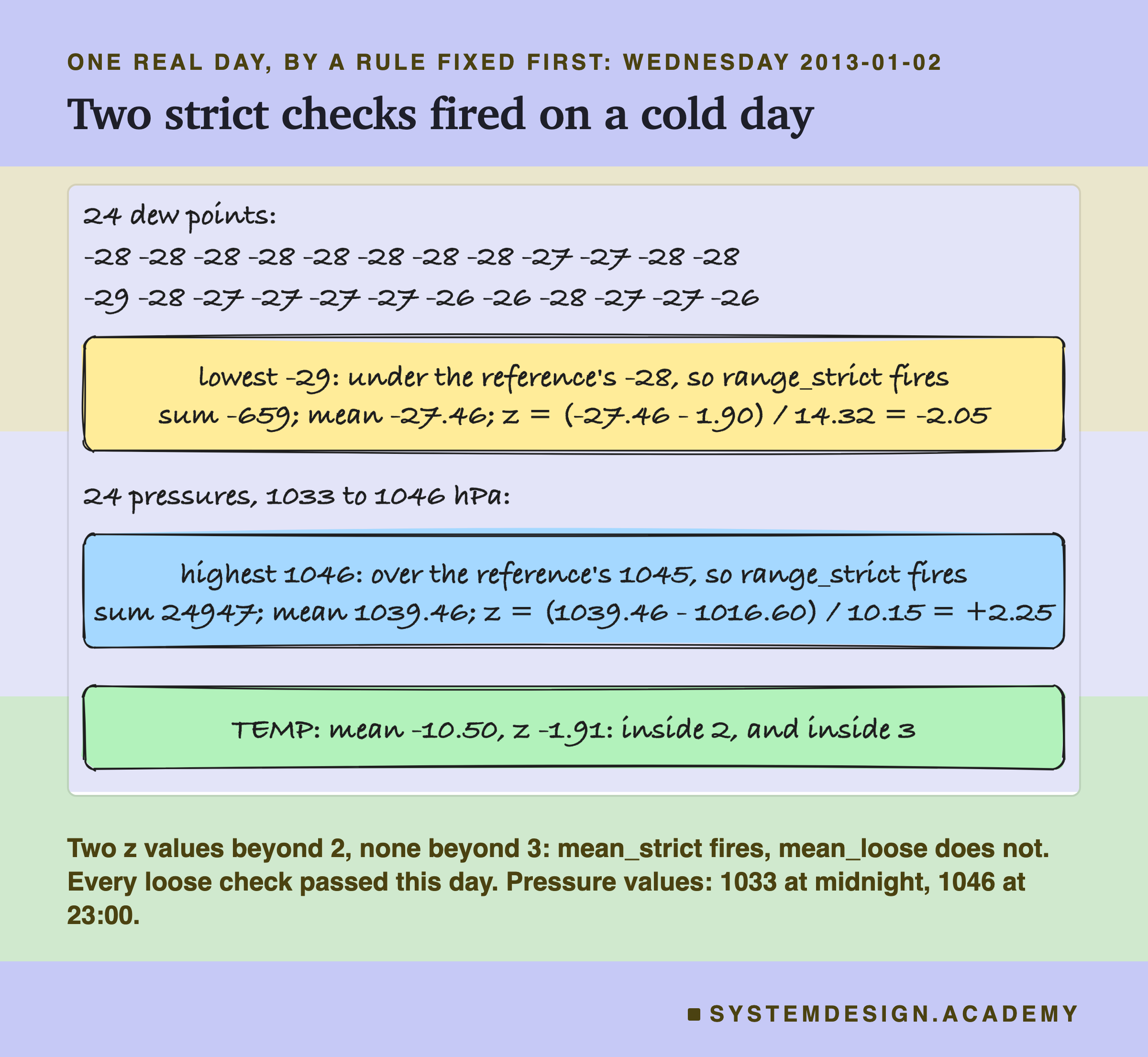
A hand-drawn worked day headed one real day, by a rule fixed first: Wednesday 2013-01-02, titled two strict checks fired on a cold day. 24 dew points: -28 -28 -28 -28 -28 -28 -28 -28 -27 -27 -28 -28, then -29 -28 -27 -27 -27 -27 -26 -26 -28 -27 -27 -26. A box: lowest -29: under the reference's -28, so range_strict fires; sum -659; mean -27.46; z, (-27.46 - 1.90) / 14.32, is -2.05. Then 24 pressures, 1033 to 1046 hPa. A box: highest 1046: over the reference's 1045, so range_strict fires; sum 24947; mean 1039.46; z, (1039.46 - 1016.60) / 10.15, is +2.25. A box: TEMP: mean -10.50, z -1.91: inside 2, and inside 3. Beneath: two z values beyond 2, none beyond 3: mean_strict fires, mean_loose does not; every loose check passed this day; pressure values: 1033 at midnight, 1046 at 23:00.

Start with the range check. The day's 24 dew points run from -29 to -26. The lowest dew point in the three reference years was -28. So at noon, the dew point went one degree below anything the reference had seen, and the strict range check fired. The day's pressure rose from 1033 at midnight to 1046 at 23:00. The reference's highest was 1045, so pressure broke it too.

Now the mean check. The 24 dew points add up to -659. Divided by 24, that is a mean of -27.46. The reference days' mean dew point was 1.90, with a standard deviation of 14.32. The z-score says how many standard deviations a value sits from the mean: -27.46 minus 1.90, divided by 14.32, is -2.05.

Pressure works the same way. The 24 pressures add up to 24,947, a mean of 1039.46. Against a reference mean of 1016.60 and a standard deviation of 10.15, the z-score is +2.25. Temperature's z-score was -1.91.

Map the pencil work onto the demo. The range test is d[c].between(LO[c], HI[c]) for each row. Adding up and dividing by 24 is g.mean(). Taking away the mean and dividing by the spread is (g.mean() - MU) / SD. The script does the same arithmetic for every day at once.

Two z-scores are beyond 2, and none is beyond 3. So the strict mean check fired and the loose one did not. Every loose check passed this day. This was a very cold, very dry winter day: real weather, not a fault.

The Code, Part by Part

Loading. fetch_openml(data_id=42891) downloads the data once and reads the local copy after that. The wind code comes back as pandas text, so the script turns it into plain strings. day is the date of each hour, built from the year, month and day columns. ref is 2010 to 2012 and srv is 2013 and 2014.

The frozen profile. CATS is the list of wind codes the reference has. LO and HI are each sensor's lowest and highest value in the reference. day_means is each reference day's average of each sensor; MU and SD are the mean and standard deviation of those averages. Everything the checks know comes from these five names.

fault(d, kind). Takes a copy of the rows and puts in one fault. For sentinel, it gives every row a random key from numpy.random.default_rng(0) and marks the three smallest keys of each day. For stuck, transform("first") gives every row its day's first dew point.

How to Add Checks, Step by Step
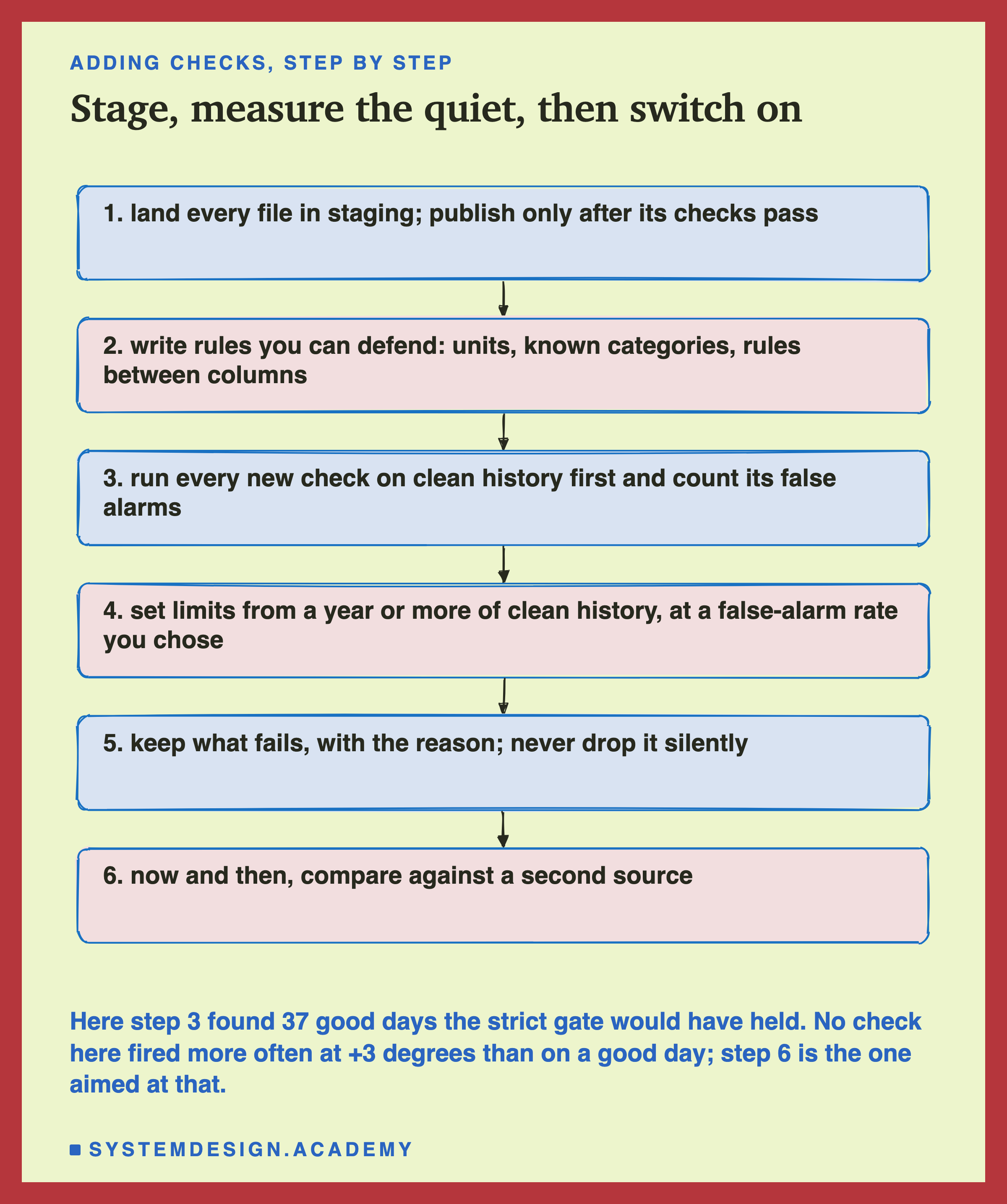
A hand-sketched column of six boxes joined by arrows, headed adding checks, step by step, titled stage, measure the quiet, then switch on. 1, land every file in staging; publish only after its checks pass. 2, write rules you can defend: units, known categories, rules between columns. 3, run every new check on clean history first and count its false alarms. 4, set limits from a year or more of clean history, at a false-alarm rate you chose. 5, keep what fails, with the reason; never drop it silently. 6, now and then, compare against a second source. Beneath: here step 3 found 37 good days the strict gate would have held; no check here fired more often at +3 degrees than on a good day; step 6 is the one aimed at that.

Land every file in staging first. Publish it to the shared table only after its checks pass. In Iceberg that is an audit branch; in a plain folder it can be a staging path.

Write rules you can defend. A known unit, a known list of categories, and a rule between columns, such as dew point not above air temperature. Together with the loose stuck check, these caught every fault here except the offset, and none of them fired on a clean day. Several of those catches were certain by arithmetic, so treat that as a floor on what such rules do, not a ceiling.

Run every new check on clean history first. Count how often it fires on days you know were fine. Here that would have shown the strict gate holding 37 good days before it ever went live.

Set each limit from at least a year of clean history, and choose a false-alarm rate you can live with. A month misses the seasons: here, a January would have set very different limits from a July. And zero false alarms is not the goal, because the quietest setting also misses the most. Write down the rate you chose, and why. A limit with a written reason can be reviewed. A limit copied from last year's minimum cannot.

Keep what fails, with the reason. Put it in a quarantine table that you add to on every run, with the batch id and a timestamp. dbt's store_failures table is replaced on each run, so copy from it rather than keep it.

Run the checks in CI too. CI, continuous integration, runs tests on every code change. If someone edits a transform or a check, run the suite on a sample of real data before the change merges.

It is the only step aimed at a value that is wrong but normal, like the thermometer 3 degrees high.

When a Check Earns Its Place
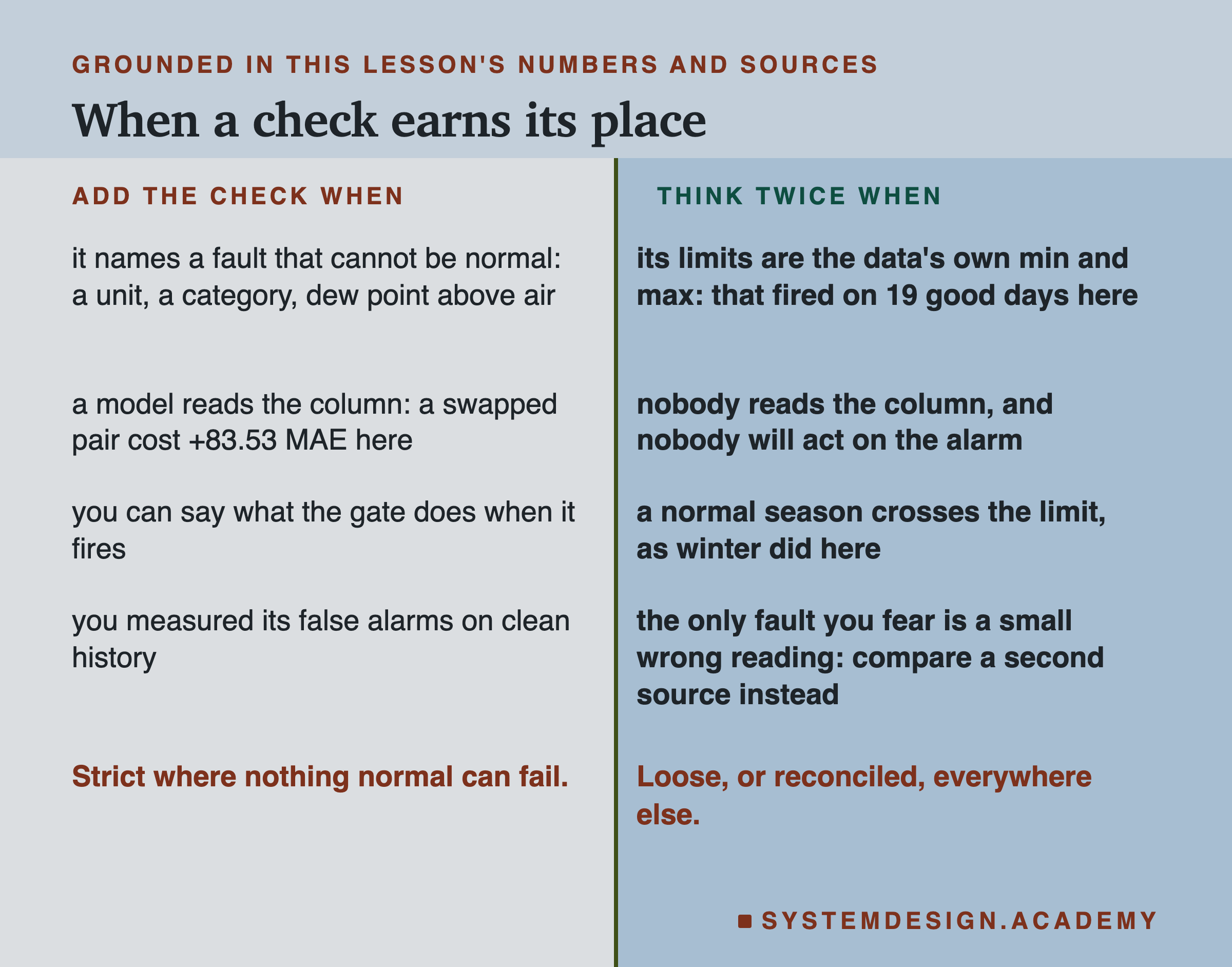
A two-column table headed grounded in this lesson's numbers and sources, titled when a check earns its place. Left, add the check when: it names a fault that cannot be normal: a unit, a category, dew point above air; a model reads the column: a swapped pair cost +83.53 MAE here; you can say what the gate does when it fires; you measured its false alarms on clean history. Right, think twice when: its limits are the data's own min and max: that fired on 19 good days here; nobody reads the column, and nobody will act on the alarm; a normal season crosses the limit, as winter did here; the only fault you fear is a small wrong reading: compare a second source instead. Beneath: strict where nothing normal can fail; loose, or reconciled, everywhere else.

Add the check when it names a fault that cannot be normal. A unit, a known category, or dew point above air temperature. Here those rules, with the loose stuck check, caught every fault except the offset and never fired on a clean day. Some of those catches were certain by arithmetic.

Add it when a model reads the column. The swap cost 83.53 MAE here, and one rule between two columns caught it every day.

Add it when you can say what the gate does when it fires. Hold the file, set rows aside, or tell a person. A check with no action is a comment.

Add it once you have measured its false alarms on clean history. Then you know what it costs before it pages anyone.

Think twice when its limits are the data's own minimum and maximum. Here that fired on 19 good days in two years.

Think twice when nobody reads the column, or nobody will act on the alarm. Think twice when a normal season crosses the limit, as the cold snaps did here.

Think twice when the only fault you fear is a small wrong reading. No band will see it. Compare against a second source instead.

What These Numbers Can and Cannot Tell You
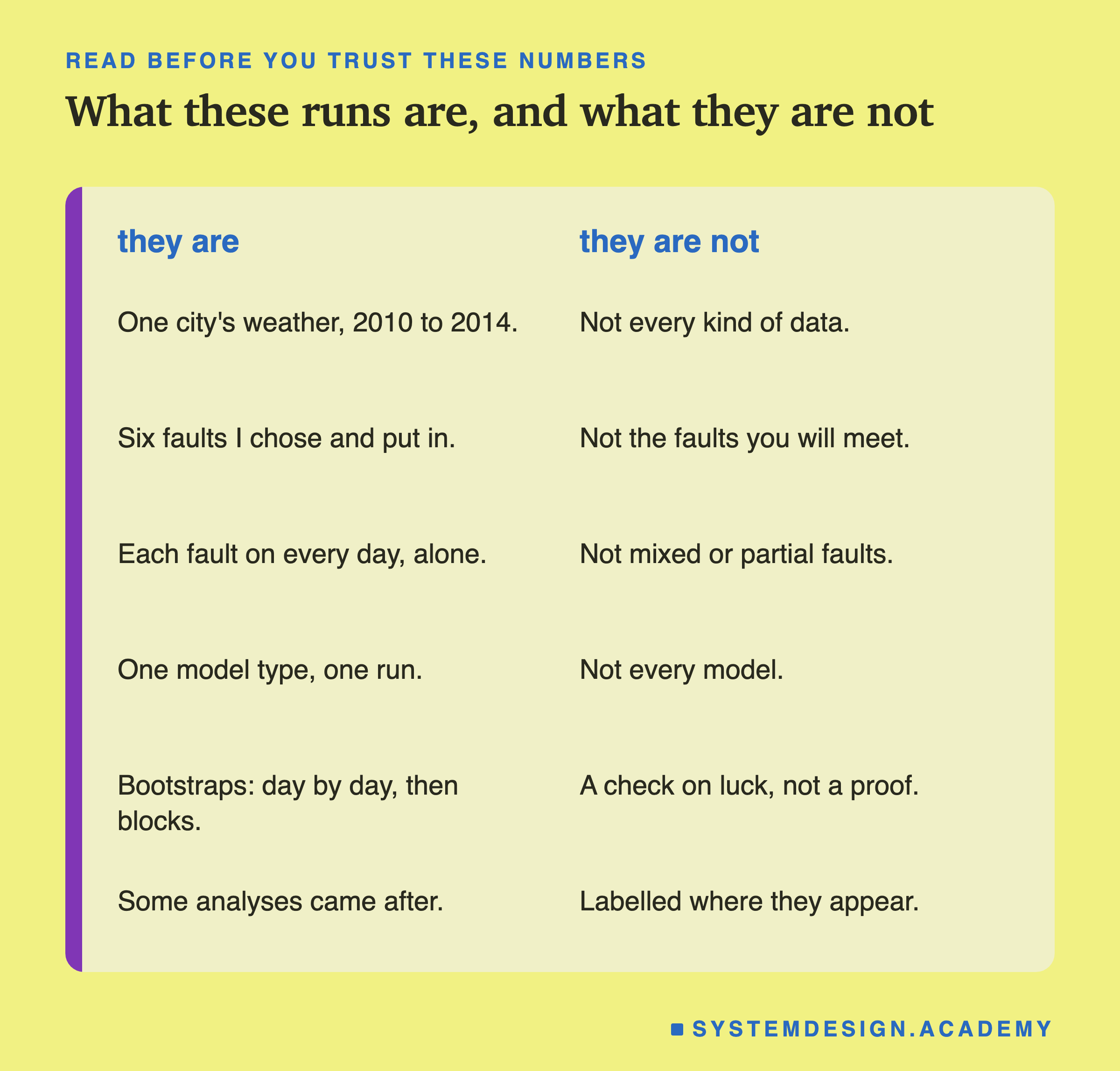
A two-column page headed read before you trust these numbers, titled what these runs are, and what they are not. They are: one city's weather, 2010 to 2014; six faults I chose and put in; each fault on every day, alone; one model type, one run; bootstraps: day by day, then blocks; some analyses came after. They are not: not every kind of data; not the faults you will meet; not mixed or partial faults; not every model; a check on luck, not a proof; labelled where they appear.

One city's weather, 2010 to 2014. Everything here is one dataset with three sensors and a wind code. Other data, with other columns and other seasons, will give other rates.

Six faults I chose and put in. Real faults are messier. I built several checks with one of these faults in mind, so their catches were expected. The false alarms, the partial catches and the offset were not.

Each fault on every day, alone. Real faults come and go, arrive together, and touch part of a day. This lab did not test any of that.

One model type, one run. The costs are for one kind of model. A linear model, which reads a pressure of 101 very differently from a tree, could suffer far more.

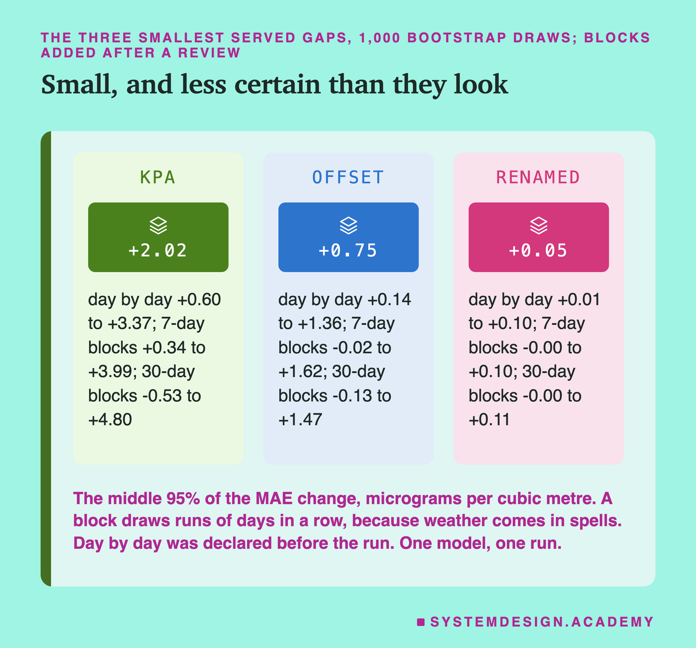
The bootstraps check luck, and nothing else. They ask whether another draw of days from the same two years would agree. The day-by-day one treats each day as unrelated to the next, and weather runs in spells. With 7-day and 30-day blocks, the three smallest gaps could not be told apart from zero. Neither says anything about another city or another year.

Some analyses came after the results. The swap check, the reasons for the false alarms, the rename details, the offset sweep and the one day were designed after I saw the first results. I wrote them into the report's docstring before it first ran, and every figure that shows them says so. The faults on both sides, the block bootstrap, the scattered-rows arithmetic and the 1-degree dew point rule came later still, after a review of this lesson.

What to Do Next
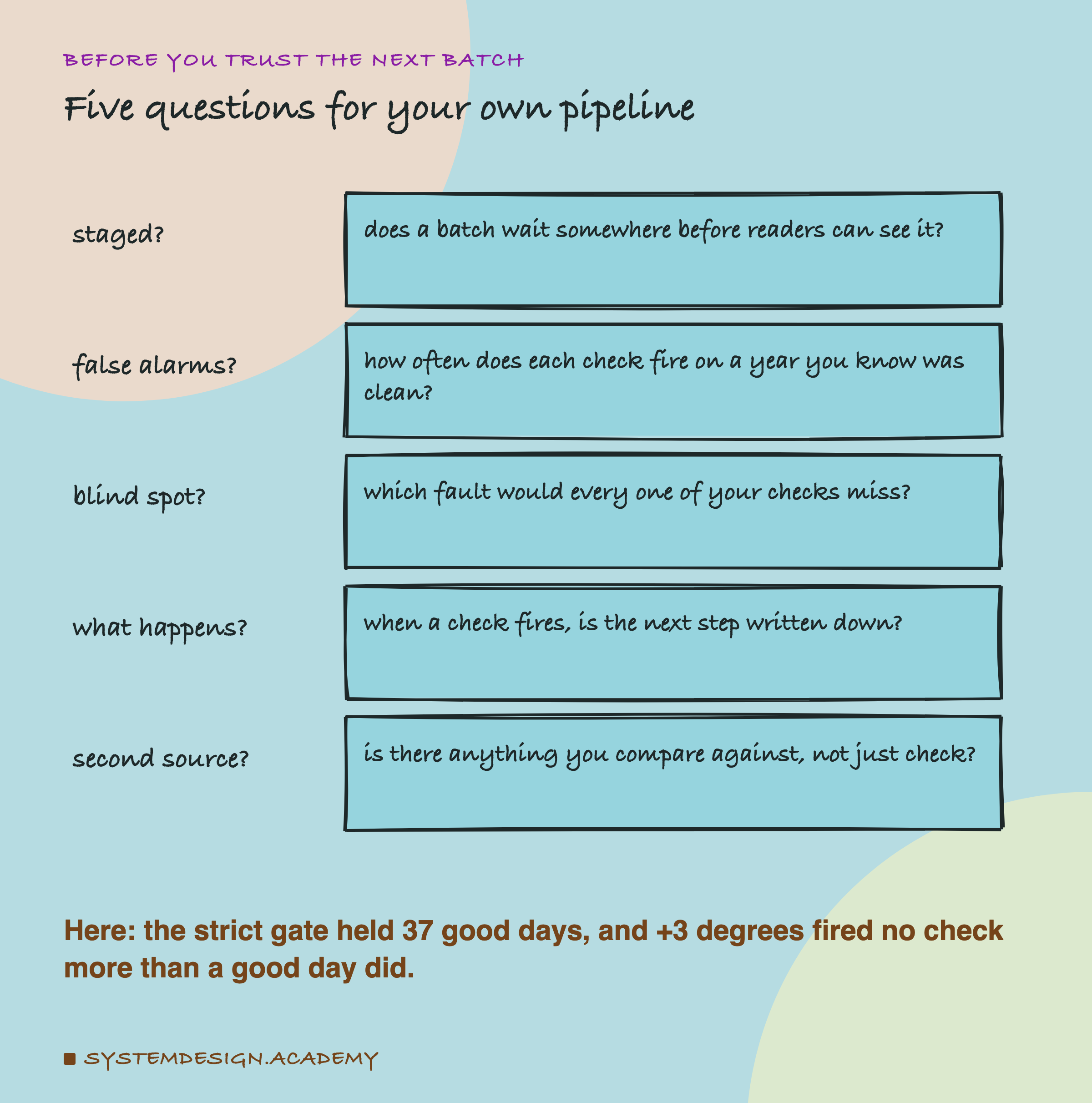
A hand-drawn list headed before you trust the next batch, titled five questions for your own pipeline. Staged?: does a batch wait somewhere before readers can see it? False alarms?: how often does each check fire on a year you know was clean? Blind spot?: which fault would every one of your checks miss? What happens?: when a check fires, is the next step written down? Second source?: is there anything you compare against, not just check? Beneath: here, the strict gate held 37 good days, and +3 degrees fired no check more than a good day did.

Take one pipeline your team runs and ask the five questions on the card. The quickest are the first and the third. Does a batch wait anywhere before readers can see it? And which fault would every one of your checks miss? If you cannot name one, you have not looked yet.

Then do the measurement. Take at least a year of history you trust, and run your checks on it. Count how often each one fires. Then put one fault of your own into a copy, and count again. Here that showed a strict gate holding 37 good days, and no check firing more often on a 3 degree error than on a good day.
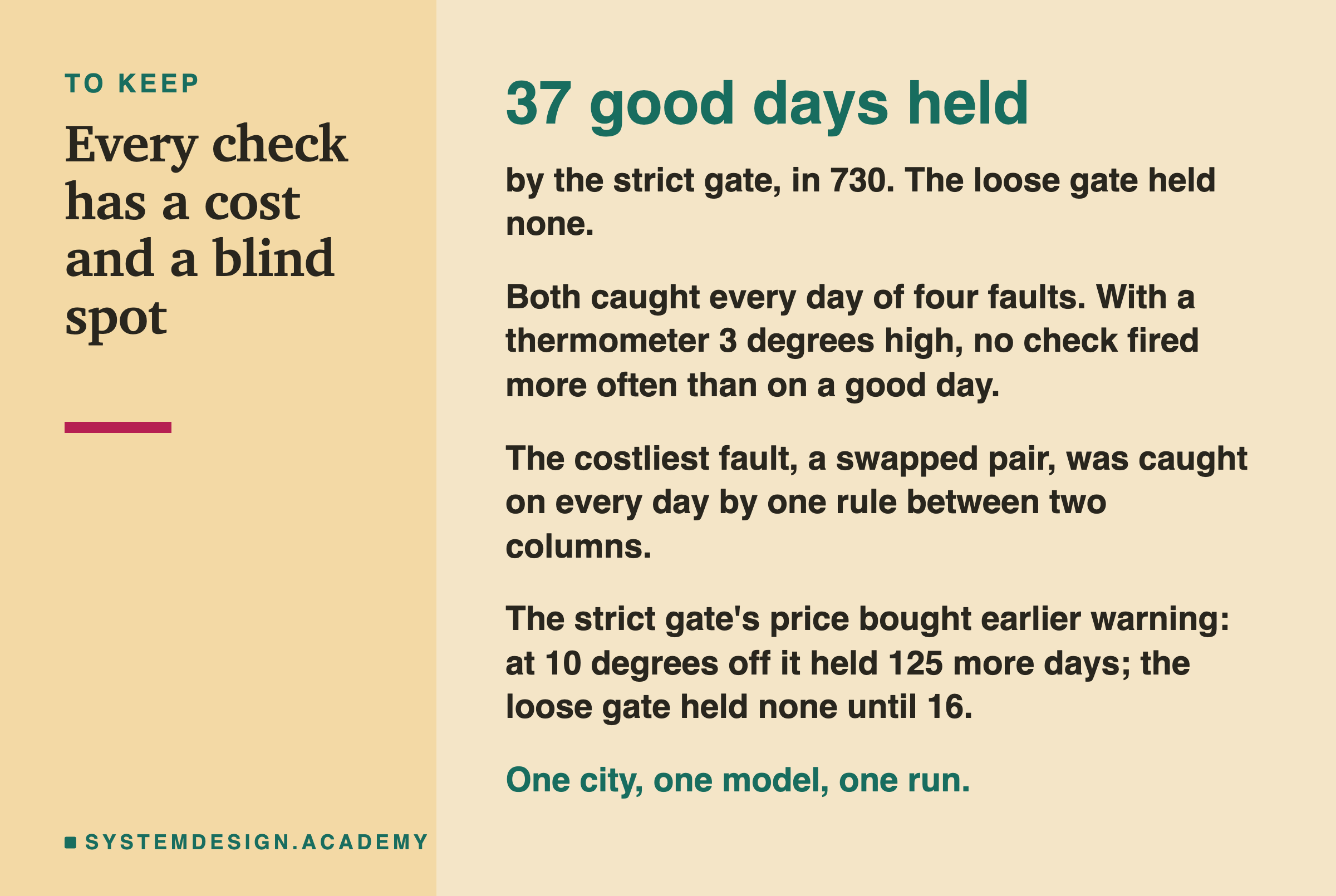
A closing card headed to keep, titled every check has a cost and a blind spot. In large type: 37 good days held. Beneath: by the strict gate, in 730; the loose gate held none. Then: both caught every day of four faults; with a thermometer 3 degrees high, no check fired more often than on a good day. Then: the costliest fault, a swapped pair, was caught on every day by one rule between two columns. Then: the strict gate's price bought earlier warning: at 10 degrees off it held 125 more days; the loose gate held none until 16. Last: one city, one model, one run.

The card keeps the lesson's numbers. The strict gate held 37 good days in two years, and the loose gate held none. Both caught every day of four faults. With the thermometer reading 3 degrees high, no check fired more often than on a good day. The costliest fault, the swap, was caught every day by one rule between two columns. And the strict gate's false alarms bought something: at 10 degrees off it held 125 more days, while the loose gate held none until 16.

The next lesson in this chapter is about data versioning. It covers how to pin the exact data a model was trained on, with tools such as DVC, LakeFS and table time travel. Then a batch you fixed and loaded again can be traced.

Knowledge Check

Knowledge Check

4 questions - Score 80% to pass

Q1

In the lab, no check fired on a thermometer reading 3 degrees high more often than on a clean day. Why?

Q2

The strict gate held 37 of the 730 clean serving days. What was behind those days?

Q3

TEMP and DEWP arrived in each other's columns. Which check caught it on all 730 days?

Q4

In Great Expectations 1.23.2, what happens when an expectation fails during batch.validate()?
Zoom in on one batch at run time and you can see where the decision happens. The checks run, the passing rows go to the table, the failing ones go to quarantine with their reason, and a report is posted.

The old version of this lesson said that when a critical check fails, Great Expectations "raises a GreatExpectationsError". It does not. I ran it: a failed check returns a result whose success is False, and nothing is raised. The error comes from the Great Expectations operators for Apache Airflow, a scheduler for data jobs. Their code raises GXValidationFailed when result.success is false, so the task fails.

TensorFlow Data Validation computes statistics for each column and compares datasets. Its guide says it measures drift with "L-infinity distance for categorical features and approximate Jensen-Shannon divergence for numeric features", and that you set the threshold. It is part of Google's TFX pipelines, but it also reads pandas tables and CSV files. Deequ, from Amazon, is "a library built on top of Apache Spark for defining 'unit tests for data'". dbt, a tool for transforms, ships four tests: unique, not_null, accepted_values and relationships.

The old version of this lesson showed Great Expectations code for an older version. In 1.x the context has no sources attribute, and a batch has no expect_... methods. So I rewrote it. The script below writes five of the lab's checks in both tools. It runs them on one real day, 2 January 2013, and on the same day with two columns swapped. I ran it with great_expectations 1.23.2 and pandera 0.33.1, in their own virtual environment.

"""The lab's checks written in Great Expectations and Pandera, run on one real day.

Lesson 5 of 'Data Engineering for ML'. It needs great_expectations and
pandera (pip install great_expectations pandera scikit-learn). I ran it
with great_expectations 1.23.2 and pandera 0.33.1 in their own virtual
environment, apart from the lab's.
    python dq_tools_check.py out.json

Design, written 2026-09-30 before it ran: take one clean serving day of
Beijing PM2.5, 2013-01-02 (the day the report's rule picked), and the same
day with TEMP and DEWP swapped. Run five of the lab's checks on both, in
each tool: range_loose, category, consistency, stuck_loose and
mean_loose, with the limits the lab's report stored. Record what each
tool says for each check, and compare it with the lab's own answer for
that day, which the report stores.
After the first run: I had written here that on the swapped day only
consistency would fire. That was my guess, not the lab's answer, and it
was wrong: the swapped TEMP column's mean is more than 3 standard
deviations from TEMP's reference, and the lab says so too. The checks
also got names, so a failure says which rule broke. Added after that run,
before it ran: pandera's infer_schema on the reference years, 2010 to
2012, to see which limits it writes by itself. That part also needs
scikit-learn, for the download. Added next, also before it ran: the same
day with TEMP = -999 at the three hours the lab's draw picked, against
the loose TEMP range, once with mostly at its default and once at 0.85.

Author: Roni Das
Created: 2026-09-30
"""
import json
import sys
from pathlib import Path

import pandas as pd

HERE = Path(__file__).resolve().parent
R = json.load(open(HERE.parent / "results" / "dq-report.json"))
P = R["profile"]
day = pd.DataFrame(R["one_day"]["rows"])
swapped = day.assign(TEMP=day["DEWP"], DEWP=day["TEMP"])
# mean_loose: the day's mean within 3 standard deviations of the reference
MEAN = {c: (P["mu"][c] - 3 * P["sd"][c], P["mu"][c] + 3 * P["sd"][c])
        for c in ("DEWP", "TEMP", "PRES")}
out = {"day": R["one_day"]["day"]}

# ---- Great Expectations ----
import great_expectations as gx
import great_expectations.expectations as gxe

context = gx.get_context(mode="ephemeral")
batches = (context.data_sources.add_pandas("feed")
           .add_dataframe_asset("weather_day")
           .add_batch_definition_whole_dataframe("one_day"))
suite = context.suites.add(gx.ExpectationSuite(name="weather"))
for c, (lo, hi) in {"DEWP": (-60, 60), "TEMP": (-60, 60),
                    "PRES": (900, 1100)}.items():
    suite.add_expectation(gxe.ExpectColumnValuesToBeBetween(
        column=c, min_value=lo, max_value=hi))
    suite.add_expectation(gxe.ExpectColumnUniqueValueCountToBeBetween(
        column=c, min_value=2))
    suite.add_expectation(gxe.ExpectColumnMeanToBeBetween(
        column=c, min_value=MEAN[c][0], max_value=MEAN[c][1]))
suite.add_expectation(gxe.ExpectColumnValuesToBeInSet(
    column="cbwd", value_set=P["cats"]))
suite.add_expectation(gxe.ExpectColumnPairValuesAToBeGreaterThanB(
    column_A="TEMP", column_B="DEWP", or_equal=True))

out["great_expectations"] = {"version": gx.__version__}
for name, frame in (("clean", day), ("swapped", swapped)):
    batch = batches.get_batch(batch_parameters={"dataframe": frame})
    result = batch.validate(suite)
    out["great_expectations"][name] = {
        "success": result.success,
        "failed": [(r.expectation_config.type,
                    r.expectation_config.kwargs.get("column")
                    or r.expectation_config.kwargs.get("column_A"))
                   for r in result.results if not r.success]}

# mostly: the share of rows that must pass. Three -999 hours in 24 rows.
bad = day.copy()
bad.loc[bad["hour"].isin(R["one_day"]["sentinel_hours"]), "TEMP"] = -999
batch = batches.get_batch(batch_parameters={"dataframe": bad})
out["mostly"] = {}
for m in (None, 0.85):
    kw = {} if m is None else {"mostly": m}
    res = batch.validate(gxe.ExpectColumnValuesToBeBetween(
        column="TEMP", min_value=-60, max_value=60, **kw))
    out["mostly"][str(m)] = {"success": res.success,
                             "unexpected": res.result["unexpected_count"]}

# ---- Pandera ----
import pandera
import pandera.pandas as pa

cols = {c: pa.Column(float, [
    pa.Check.in_range(lo, hi),
    pa.Check(lambda s: s.nunique() >= 2, name="not_stuck"),
    pa.Check(lambda s, c=c: MEAN[c][0] <= s.mean() <= MEAN[c][1],
             name="mean_in_band")], coerce=True)
    for c, (lo, hi) in {"DEWP": (-60, 60), "TEMP": (-60, 60),
                        "PRES": (900, 1100)}.items()}
cols["cbwd"] = pa.Column(str, pa.Check.isin(P["cats"]))
schema = pa.DataFrameSchema(cols, checks=pa.Check(
    lambda d: d["DEWP"] <= d["TEMP"], name="dew_not_above_temp"))

out["pandera"] = {"version": pandera.__version__}
for name, frame in (("clean", day), ("swapped", swapped)):
    try:
        schema.validate(frame, lazy=True)
        out["pandera"][name] = {"success": True, "failed": []}
    except pa.errors.SchemaErrors as err:
        fc = err.failure_cases
        out["pandera"][name] = {
            "success": False, "failure_rows": len(fc),
            "failed": sorted({(str(a), str(b)) for a, b in
                              zip(fc["column"], fc["check"])}),
            "rows_failing_dew_rule": int(fc.loc[
                fc["check"] == "dew_not_above_temp", "index"].nunique()),
            "columns": list(fc.columns)}

# ---- Pandera's own guess at limits, from the reference years ----
from sklearn.datasets import fetch_openml

raw = fetch_openml(data_id=42891, as_frame=True, parser="auto").frame
ref = raw.loc[raw["year"] <= 2012, ["DEWP", "TEMP", "PRES"]].astype(float)
inferred = pa.infer_schema(ref)
out["infer_schema"] = {c: {k.name: k.statistics for k in
                           inferred.columns[c].checks} for c in ref}

LAB = {"range_loose": "range", "category": "category",
       "consistency": "consistency", "stuck_loose": "stuck",
       "mean_loose": "mean"}
out["lab_swapped_fired"] = [c for c in R["one_day"]["swapped_fired"]
                            if c in LAB]
out["lab_clean_fired"] = [c for c in R["one_day"]["fired"] if c in LAB]
for tool in ("great_expectations", "pandera"):
    print(f"{tool} {out[tool]['version']}")
    for name in ("clean", "swapped"):
        got = out[tool][name]
        rules = sorted({f[1] if tool == "pandera" else f[0]
                        for f in got["failed"]})
        print(f"  {name:<8} passed: {got['success']}")
        for rule in rules:
            print(f"    failed: {rule}")
print(f"the lab, swapped day: {', '.join(out['lab_swapped_fired'])}")
print("three -999 hours, TEMP within -60 to 60:")
for m, got in out["mostly"].items():
    name = "default" if m == "None" else m
    print(f"  mostly {name:<7} {got['unexpected']} rows out,"
          f" passed: {got['success']}")
print("pandera infer_schema, 2010 to 2012:")
for c, found in out["infer_schema"].items():
    lo = found["greater_than_or_equal_to"]["min_value"]
    hi = found["less_than_or_equal_to"]["max_value"]
    print(f"  {c}  {lo} to {hi}")
if len(sys.argv) > 1:
    json.dump(out, open(sys.argv[1], "w"), indent=1, default=str)

This is a real run of that script.

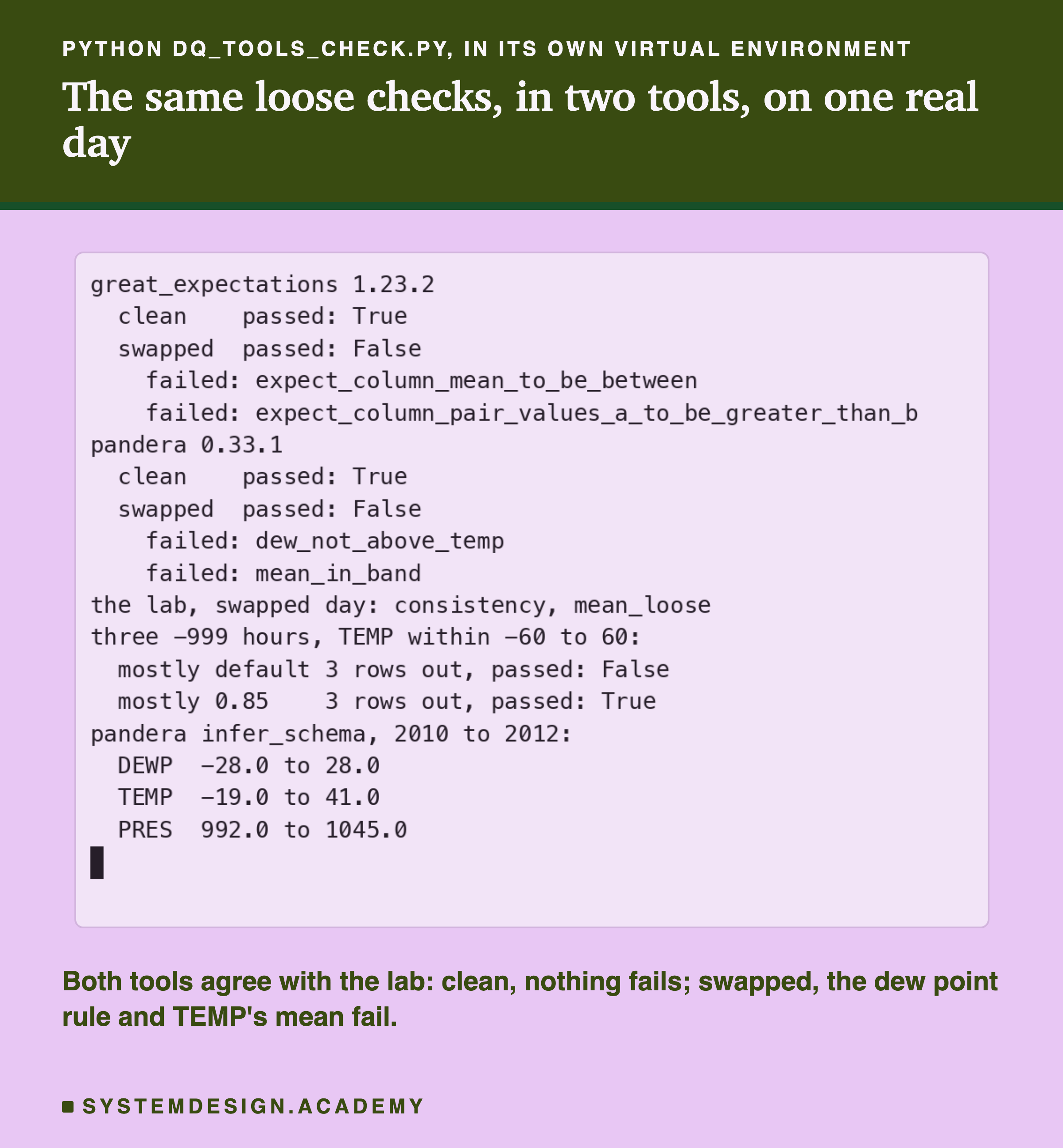
A real terminal recording of python dq_tools_check.py, headed in its own virtual environment, titled the same loose checks, in two tools, on one real day. It prints great_expectations 1.23.2; clean, passed: True; swapped, passed: False; failed: expect_column_mean_to_be_between; failed: expect_column_pair_values_a_to_be_greater_than_b. Then pandera 0.33.1; clean, passed: True; swapped, passed: False; failed: dew_not_above_temp; failed: mean_in_band. Then the lab, swapped day: consistency, mean_loose. Then three -999 hours, TEMP within -60 to 60: mostly default, 3 rows out, passed: False; mostly 0.85, 3 rows out, passed: True. Then pandera infer_schema, 2010 to 2012: DEWP -28.0 to 28.0, TEMP -19.0 to 41.0, PRES 992.0 to 1045.0. Beneath: both tools agree with the lab: clean, nothing fails; swapped, the dew point rule and TEMP's mean fail.

Both tools passed the clean day and failed the swapped one, on the same two rules the lab's loose checks fired: the dew point rule, and TEMP's mean. On that day the lab's strict range and strict mean checks fired as well. When I wrote the script's design, I had guessed only the dew point rule would fail. I was wrong, and I said so in the script. On that very cold day, the swapped TEMP column's mean sat more than 3 standard deviations from TEMP's usual.

The next three lines show the hazard in mostly. On the same day with three -999 hours, the range check failed at the default and passed at 0.85. A loose mostly lets a sentinel day through.

Here is how each of the lab's five loose checks looks in each tool, so you can find it in the code above.

The range check is ExpectColumnValuesToBeBetween in Great Expectations, and Check.in_range in Pandera. Both include the two limits by default.

The category check is ExpectColumnValuesToBeInSet, and Check.isin. Each takes the list of known wind codes from the reference years.

The dew point rule is ExpectColumnPairValuesAToBeGreaterThanB with or_equal=True: column A is TEMP and column B is DEWP. In Pandera it is a check on the whole table rather than one column. Pandera's docs call that a wide check. Mine returns one True or False per row.

The stuck check is ExpectColumnUniqueValueCountToBeBetween with a lowest count of 2. In Pandera I wrote it as my own check, s.nunique() >= 2, and gave it a name so the failure says what broke.

The mean check is ExpectColumnMeanToBeBetween, with the band worked out from the reference: the mean minus 3 standard deviations to the mean plus 3. In Pandera it is another named check, on s.mean().

The last four lines matter most. Pandera's infer_schema, given the three reference years, wrote limits of -28 to 28, -19 to 41 and 992 to 1045. Those are exactly the limits of the lab's strict range check. The lab measures what those limits cost.

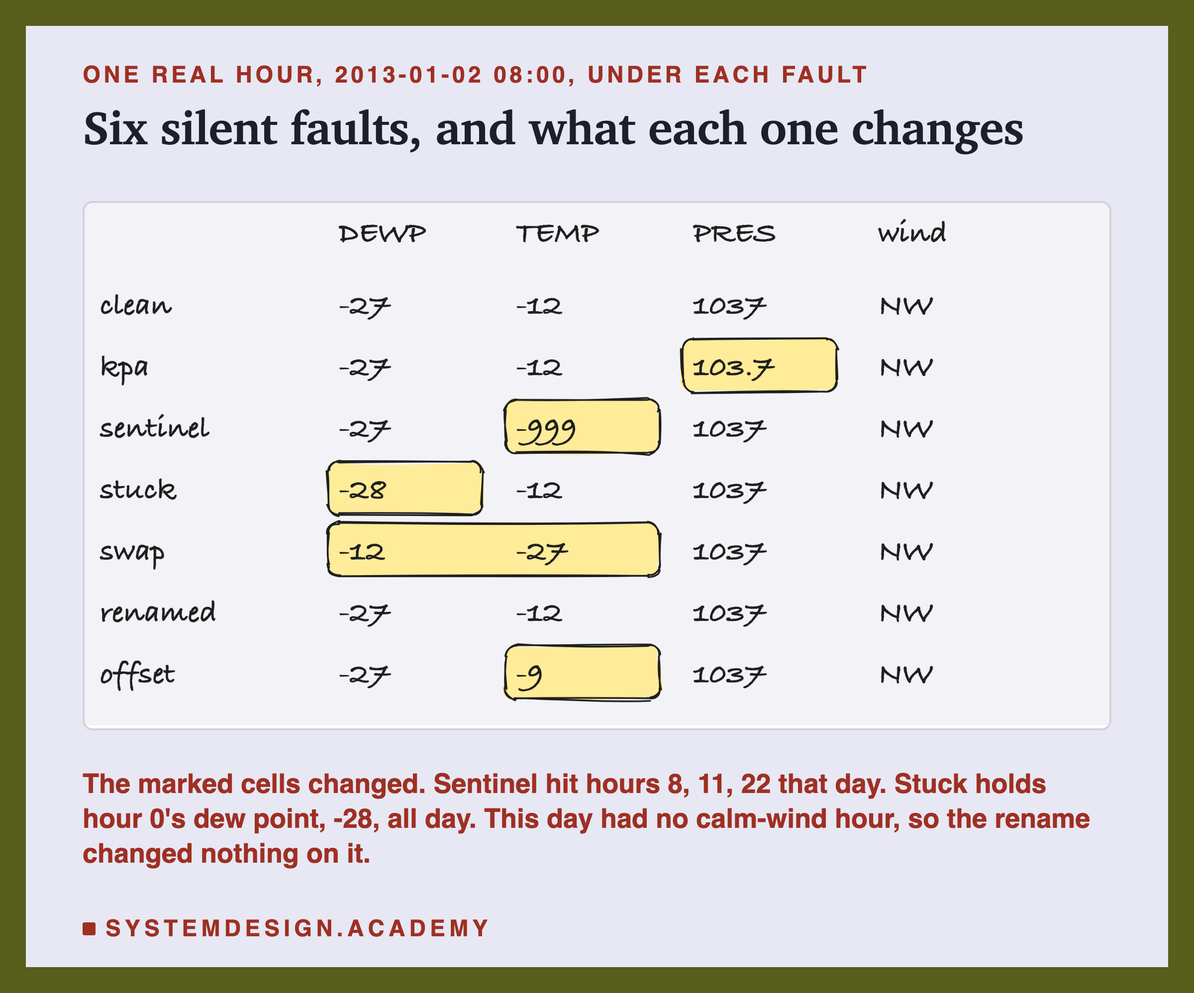
A hand-drawn table headed one real hour, 2013-01-02 08:00, under each fault, titled six silent faults, and what each one changes. Columns DEWP, TEMP, PRES, wind. Clean: -27, -12, 1037, NW. Kpa: -27, -12, 103.7, NW, with the pressure marked. Sentinel: -27, -999, 1037, NW, with the temperature marked. Stuck: -28, -12, 1037, NW, with the dew point marked. Swap: -12, -27, 1037, NW, with dew point and temperature marked together. Renamed: -27, -12, 1037, NW. Offset: -27, -9, 1037, NW, with the temperature marked. Beneath: the marked cells changed; sentinel hit hours 8, 11, 22 that day; stuck holds hour 0's dew point, -28, all day; this day had no calm-wind hour, so the rename changed nothing on it.

Here is what each fault does. kpa: the pressure arrives in kilopascals instead of hectopascals, so every value is divided by 10. sentinel: three random hours of each day carry a temperature of -999, the kind of code a feed uses for "no reading". stuck: the dew point sensor freezes at the day's first reading. swap: the temperature and dew point arrive in each other's columns. renamed: the wind code cv, for calm and variable wind, arrives as calm. offset: the thermometer reads 3 degrees too high.

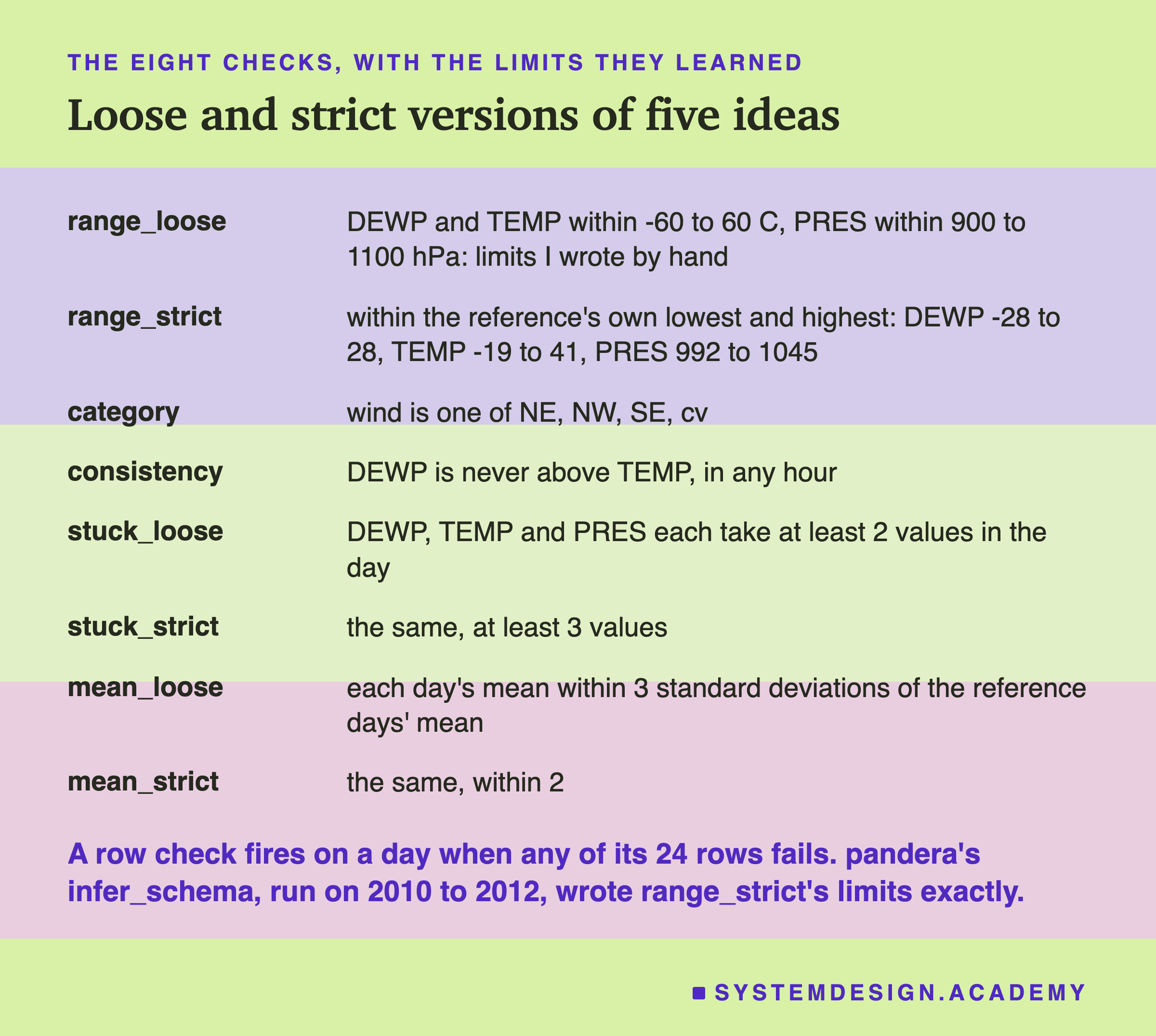
A two-column list headed the eight checks, with the limits they learned, titled loose and strict versions of five ideas. range_loose: DEWP and TEMP within -60 to 60 C, PRES within 900 to 1100 hPa: limits I wrote by hand. range_strict: within the reference's own lowest and highest: DEWP -28 to 28, TEMP -19 to 41, PRES 992 to 1045. category: wind is one of NE, NW, SE, cv. consistency: DEWP is never above TEMP, in any hour. stuck_loose: DEWP, TEMP and PRES each take at least 2 values in the day. stuck_strict: the same, at least 3 values. mean_loose: each day's mean within 3 standard deviations of the reference days' mean. mean_strict: the same, within 2. Beneath: a row check fires on a day when any of its 24 rows fails; pandera's infer_schema, run on 2010 to 2012, wrote range_strict's limits exactly.

The checks come in loose and strict versions of five ideas. The loose range limits are ones I wrote by hand, far wider than anything the reference years saw. The strict range limits are the reference's own lowest and highest values. The mean checks compare each day's average with the averages of the 1,096 reference days. A standard deviation measures how spread out those averages are. A row check fires on a day when any of the day's 24 rows fails.

Two gates combine them. The loose gate holds a day if any loose check fires. The strict gate holds a day if any strict check fires. The category and consistency checks belong to both.

This chart shows why a mean check has to be so wide. It plots each clean serving day's average temperature against the reference band. Winter and summer both belong to a normal year, so the reference days' averages are very spread out. Two standard deviations either side of 12.05 degrees is a band from about -12 to 36.

A narrower band has its own cost. At one standard deviation, TEMP's band would run from 0.25 to 23.86 degrees, and every day in this chart below 0 would fire. A band this wide cannot see a thermometer that reads 3 degrees high: it moves the whole line up by 3, and the line stays inside. I drew this chart after the results.

Three panels headed why the strict checks fired on clean days, after the results, titled real cold snaps and quiet days, not faults. Strict range: 19 days; DEWP past the reference's lowest or highest on 16, PRES on 3, TEMP on 1. Strict stuck: 12 days; under 3 values all day: DEWP on 10, TEMP on 2, PRES on 1. Strict mean: 12 days; over 2 SD: PRES on 9, DEWP on 4. Beneath: a day can fire on two columns, so the columns add up to more than the days; the first was 2013-01-02: dew point reached -29, one degree under the reference's lowest.

After the results, I looked at why each strict check fired on a clean day. The strict range check fired mostly on dew point: on 16 days the air was drier than anything in the three reference years. All 16 went below the lowest limit, none above the highest. The strict stuck check fired mostly on dew point too, on quiet days when it barely moved. The strict mean check fired mostly on pressure.

I cannot prove that none of these were faults, because the data holds one station and there is nothing to compare with. None of them tripped the loose stuck check or the dew point rule. Most likely they were real weather that the reference years happened not to contain. A range taken from the data's own minimum and maximum says "never seen before", and that is not the same as "wrong".

The third case shows which faults hurt even without a mismatch. With the fault on both sides, the kilopascals, the offset, the swap and the rename all scored 46.39, exactly clean. One likely reason: a tree only compares each value with a threshold. So a change that keeps the values in the same order, made the same way on both sides, gives the same splits. The stuck sensor still cost 53.28 on both sides, because a frozen dew point gives the model nothing to learn from. The -999 hours cost 46.62.

Some faults cost more served, and some trained. The stuck sensor cost more served: 54.85 against 49.29. The pressure in kilopascals cost more trained: 50.84 against 48.41, and all of that was the mismatch, since on both sides it cost nothing. Trained with -999 hours and fed clean days, the model scored 46.28, a little under clean. That is one run, and I did not test whether a gap that small is more than noise.

The swap scored 129.92 both ways, the same to every printed decimal. After the results, I checked every answer. The two swap runs gave the same prediction on all 17,339 hours. One possible reading: a tree trained with the two columns exchanged is the clean tree with its two column names exchanged.

Three panels headed the three smallest served gaps, 1,000 bootstrap draws, day by day declared first, blocks after a review, titled small, and less certain than they look. Kpa: +2.02; day by day +0.60 to +3.37; 7-day blocks +0.34 to +3.99; 30-day blocks -0.53 to +4.80. Offset: +0.75; day by day +0.14 to +1.36; 7-day blocks -0.02 to +1.62; 30-day blocks -0.13 to +1.47. Renamed: +0.05; day by day +0.01 to +0.10; 7-day blocks -0.00 to +0.10; 30-day blocks -0.00 to +0.11. Beneath: middle 95% of the MAE change, micrograms per cubic metre; a block draws runs of days in a row, because weather comes in spells; one model, one run.

Could the small gaps be luck, from which days happened to be in the two years? The design declared one check for this, a bootstrap. It picks 730 serving days at random, with repeats allowed, and measures the gap on them. Then it does that 1,000 times.

For all six faults, the middle 95% of the 1,000 gaps stayed above zero. Even the rename's +0.05 ran from +0.01 to +0.10. But that bootstrap draws days one at a time, as if each day were unrelated to the next, and weather runs in spells. After a review, I added a block bootstrap to the report. It draws runs of 7 or 30 days in a row instead.

With 7-day blocks, the offset's interval ran from -0.02 to +1.62, and the rename's from -0.00 to +0.10. With 30-day blocks, the kilopascals ran from -0.53 to +4.80. Those include zero. So for the three smallest gaps, I cannot rule out that they come from which spells of weather fell in these two years. The three large ones, the swap, the -999 hours and the stuck sensor, stayed well above zero either way. Neither bootstrap says anything about other years, other cities or other models.

For a row check, count the failing rows. If there are fewer than your limit, set those rows aside and publish the rest. The old version of this lesson set that line at 98% of rows passing, and its diagram said 99%. Both numbers were made up, and they disagreed. The limit is a policy. Set it from at least a year of clean history, and look at which rows it would set aside.

Here that look matters. On clean days, the strict range check failed 117 of 17,520 rows. 103 of them were very dry hours, with dew point below the reference years' lowest. 13 had a pressure outside the reference's range, and 1 was an hour at 42 degrees. As far as one station can tell, all of it was real weather, and setting those rows aside would hide real hours from the model.

A rule that must always hold needs the same care. The dew point rule broke on real data once, 13 against 12 on 8 October 2010. One possible reason is that each value is rounded to a whole degree. A 1-degree allowance, dew point above air temperature plus 1, broke on no row in five years. It still caught the swap on all 730 days.

Whatever you set aside, keep it. A failed row is evidence: it tells you which source broke, and once the source is fixed you can load it again. dbt builds this in. Its docs say that with store_failures, dbt "saves all records (up to limit) that failed the test", in "a new table with the name of the test". But the same page says "a test's results will always replace previous failures for the same test, even if that test results in no failures". So that table shows the latest run only.

For a lasting quarantine, copy the failures out after each run, with the batch id and a timestamp. A dropped row cannot be explained later.

A useful quarantine record holds four things. First, the rows themselves, exactly as they arrived. Second, the name of each check they failed. Third, the batch they came from, here the day. Fourth, when they were set aside. With those, a person can see at a glance that, say, every held row on one day failed the pressure range, and ask the feed's owner what changed. When the source is fixed, the same record tells you which batches to load again.

One common way to measure a moved distribution is the population stability index, or PSI. Split the values into buckets. For each bucket, take the share now minus the share in training, times the natural log of the share now divided by the share in training. Add up the buckets.

A hand-drawn worked example headed a worked example, not the lab's data, titled the population stability index, by hand. Two boxes: bucket A, 50% in training, 70% now, (0.7 - 0.5) x ln(0.7 / 0.5), which is 0.2 x 0.336, which is 0.067; bucket B, 50% in training, 30% now, (0.3 - 0.5) x ln(0.3 / 0.5), which is -0.2 x -0.511, which is 0.102. Below, a scale with marks at 0.10 and 0.25 and a dot labelled sum 0.169 between them, over the words little change, moderate, and significant, act. Beneath: the bands are a rule of thumb from credit scoring; Yurdakul and Naranjo note they are used without reference to any error rate.

Here is a small worked case, not from the lab. Two buckets had 50% each in training and 70% and 30% now. The first bucket gives 0.2 times 0.336, which is 0.067. The second gives -0.2 times -0.511, which is 0.102. The sum is 0.169.

The old version of this lesson said a PSI "above roughly zero point two flags a meaningful shift". The common rule of thumb is different. Yurdakul and Naranjo, writing in 2020, report the rule that banks use in practice. Below 0.10 means "a little change", 0.10 to 0.25 "a moderate change", and above 0.25 "a significant change, action required".

They note that "these benchmarks are used without reference to statistical type I or type II error rates", and their paper sets out to fill that gap. So the cut-offs were not chosen for a known rate of false alarms or misses. 0.169 falls in the moderate band, and a lab like the one above is one way to find out what a threshold costs on your data.

The lab's mean check had one weakness that a better profile could fix. It compared every day with the whole reference year, so winter and summer made its band very wide. One idea I did not test is to compare each day with the same month of the reference years. The band would be narrower. It might catch smaller errors, and it might also add false alarms. The way to know is to run it on clean history, as this lab did.

The guard against skew is to run the same checks, with the same frozen profile, on training data and on serving data. Google's Breck and others give a real case. Google Play's app store "discovered a few features that were always missing from the logs, but always present in training". Removing that skew "improved the app install rate on the main landing page of the app store by 2%". In this lab the swap was a skew of its own: served to a clean model, it cost 83.53 MAE.

Amazon. Deequ "is being used internally at Amazon for verifying the quality of many large production datasets", and "in error cases, dataset publication can be stopped". Google and Uber both write about false alarms. For your own checks, you have to measure that trade yourself.

This is a real run in VS Code's terminal (python validation_demo.py).

A real screenshot of VS Code's terminal after running python validation_demo.py. It prints scikit-learn 1.9.1, pandas 3.0.6; rows 43,824; days: reference 1,096, serving 730; false alarms, of 730 clean days: range_loose 0.0%, range_strict 2.6%, category 0.0%, consistency 0.0%, stuck_loose 0.0%, stuck_strict 1.6%, mean_loose 0.0%, mean_strict 1.6%; a table of faulty days caught, in percent, for kpa, sentinel, stuck, swap, renamed and offset; gates: loose 0.0% held, then 0% 0% 0% 0% 5% 100% let through; strict 5.1% held, then 0% 0% 0% 0% 4% 95%; MAE, micrograms per m3, clean 46.4, then served and trained for each fault: kpa 48.4 and 50.8, sentinel 54.9 and 46.3, stuck 54.9 and 49.3, swap 129.9 and 129.9, renamed 46.4 and 46.4, offset 47.1 and 47.5; and pandas warnings: 2, a category it does not know.

When I ran it, it printed the versions, the row and day counts, the false alarms, the table of catches, the two gates and the MAE lines. It also printed a count of pandas warnings, a line I added after the first run. All of it matches the stored dq-demo.json, and the longest printed line was 51 characters. The report's demo mode checks every one of those lines against the file.

To try something I have not run, change z > 2 in the line days["mean_loose"], days["mean_strict"] = z > 3, z > 2 to z > 2.5. I cannot tell you what it prints, because I have not run it. The question to ask is how many false alarms go away, and whether any catch goes with them.

Four brand cards headed the tools, with their logos, titled what ran where. scikit-learn: the model, and the data download. pandas: the demo's faults and checks. NumPy: the sentinel hours and the bootstrap. Python: the report's loop-by-loop rebuild, and the box. Beneath: Great Expectations and Pandera ran in their own environment, for the tool check.

The split between the tools is deliberate. scikit-learn fitted every model. The demo puts in the faults and runs the checks with pandas. The report does both again in plain Python, one row at a time. So the check that the numbers come back uses a different method from the one that made them. Plain Python also holds the playground, because it has to run in a browser.

run_checks(d). The four row checks come first, as one True or False per row: True means the row fails. groupby(d["day"]).any() turns them into one answer per day. The stuck checks count distinct values per sensor per day. The mean checks compute each day's z-score for each sensor, and take the largest in size.

table, fit and mae. table is the feature job. It turns the wind code into a category with the reference's codes, and counts any warning pandas gives while doing it. fit trains on the hours that have a PM2.5 reading. mae scores the same kind of hours.

The gates. GATES names the checks in each gate. A gate holds a day when any of its checks fired, which is clean_days[cs].any(axis=1). A faulty day gets through when none of them fired, which is 1 minus the caught share.

The rest. It prints the false alarms, then the caught share for each check and fault. Then come the two gates, then the MAE clean, served and trained. With a file name on the command line, json.dump saves every number.

Now and then, compare against a second source.