A team ships a chatbot. The demo is great. Then the first real month of traffic arrives, and finance forwards the GPU invoice. A single NVIDIA H100 rents for roughly two to four dollars an hour. Their naive server, running one request at a time, handles maybe a handful of users per card. To serve real traffic they now need a rack of these things, and the math turns a promising feature into a project nobody can afford.

This is the quiet killer of GenAI in production. The model works. The problem is that serving it is slow and expensive in a way that ordinary web services are not. A REST endpoint returns in a few milliseconds and one server handles thousands of users. An LLM chews on each request for seconds and one expensive GPU handles a few users at a time, unless you optimize it hard.

Here is the good news, and it is the whole reason this lesson exists. The gap between a naive server and a tuned one is not 20 percent. It is often 10 to 20 times more throughput on the exact same hardware, which means 10 to 20 times lower cost per token with no change to the model at all. That gap is entirely engineering: the KV cache, continuous batching, PagedAttention, quantization, and speculative decoding. Every one of them is a lever you control, and by the end of this lesson you will know what each does, roughly what it buys, and what it costs.

The model is fixed. Your GPU bill is not. It is set by how well you serve, and that is a platform problem, not a modeling one.

We will work from the ground up. First the one hardware fact that explains everything, then the memory that dominates the card, then the batching and memory tricks that deliver most of the win, then quantization and speculative decoding on top, and finally the runtimes that package all of it so you do not write a line of it yourself.

To fix inference you have to understand why it is slow in the first place, and the answer is the word autoregressive. A large language model generates text one token at a time, and each new token depends on all the tokens before it. It cannot jump ahead. To write a 500-token answer it must run the full model 500 times in sequence. There is no way to parallelize across the tokens of a single reply, because token 200 literally does not exist until token 199 has been produced and fed back in.

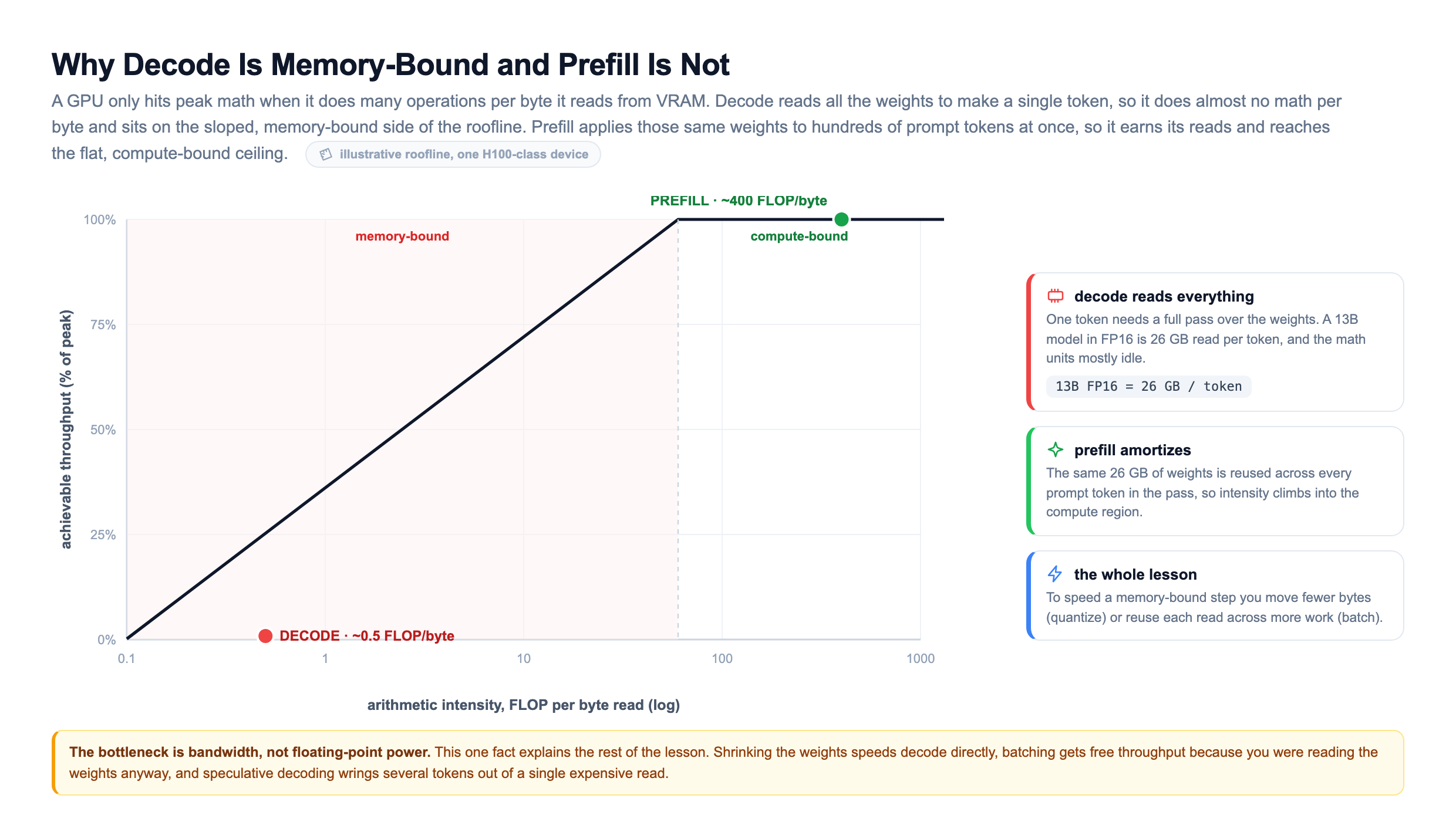
Now the surprising part, and the fact the rest of the lesson hangs on. Each of those steps is not compute-bound, it is memory-bound. On every step the GPU has to read the entire set of model weights out of VRAM to produce a single token. For a 13-billion-parameter model in FP16 that is 26 gigabytes of reading, per token. The GPU's thousands of math units sit mostly idle, starved, waiting on the memory system. The bottleneck is memory bandwidth, how fast you can move weights out of VRAM, not raw floating-point power.

Engineers formalize this with a roofline. A device only reaches its peak math rate when a workload does enough arithmetic per byte it reads. Decode does almost none, so it lives on the sloped, bandwidth-limited side. Prefill, which processes the whole prompt at once, reuses each weight across hundreds of tokens and climbs into the flat, compute-limited region.

That single fact explains almost every optimization in this lesson:

• If decode is limited by moving bytes, then shrinking the weights (quantization) makes it faster, because there are fewer bytes to move.
• If you are reading the weights anyway, then applying them to many requests at once (batching) is nearly free extra throughput, because the expensive read is already paid for.
• If each slow step only makes one token, then making the big model produce several tokens per step (speculative decoding) is a direct win against the sequential bottleneck.

Hold onto the roofline as you read on. Every technique below is either moving fewer bytes or wringing more useful work out of each byte you were already forced to read.

Before the optimizations, split a single request into its two phases, because they behave nothing alike and confusing them will mislead every performance decision you make.

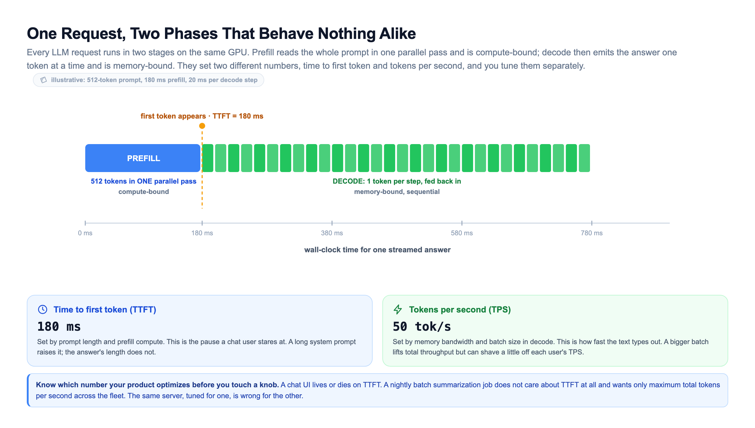
Prefill processes the entire prompt at once. All 512 prompt tokens go through the model in one big parallel pass. This phase is compute-bound, it lives in the healthy part of the roofline, and it is what you wait on before the first word appears. A longer prompt means a slower start, because there is more prompt to push through that first pass.

Decode then generates the answer one token at a time, feeding each output back in as the next input. This phase is the memory-bound, sequential grind, and it sets how fast the text streams out after it begins.

Those two phases map onto the two numbers you actually report to users and to your capacity planning:

If a model must look at every previous token to produce the next one, then naively it would recompute the attention over the entire history on every single step. Step 100 would redo the work of steps 1 through 99, step 101 would redo 1 through 100, and so on. That would make generation quadratically slow in the length of the output, which no production system could tolerate.

Instead, every model uses a KV cache. Attention works by turning each token into a key and a value. Once you have computed the key and value for a token, they never change, because the token behind them never changes. So you compute them once and cache them in VRAM. On each new step the model only computes the key and value for the one new token and reuses everything cached for the past. The quadratic recomputation problem collapses to linear work.

But this cache has a cost, and it is the single most important number in LLM serving: the KV cache lives in VRAM, and it grows with every token, for every concurrent request. For a model like Llama-2 13B, the KV cache runs on the order of 1 megabyte per token of context. Multiply that by a few thousand tokens of context and by dozens of concurrent users and the cache can easily eat more VRAM than the model weights themselves.

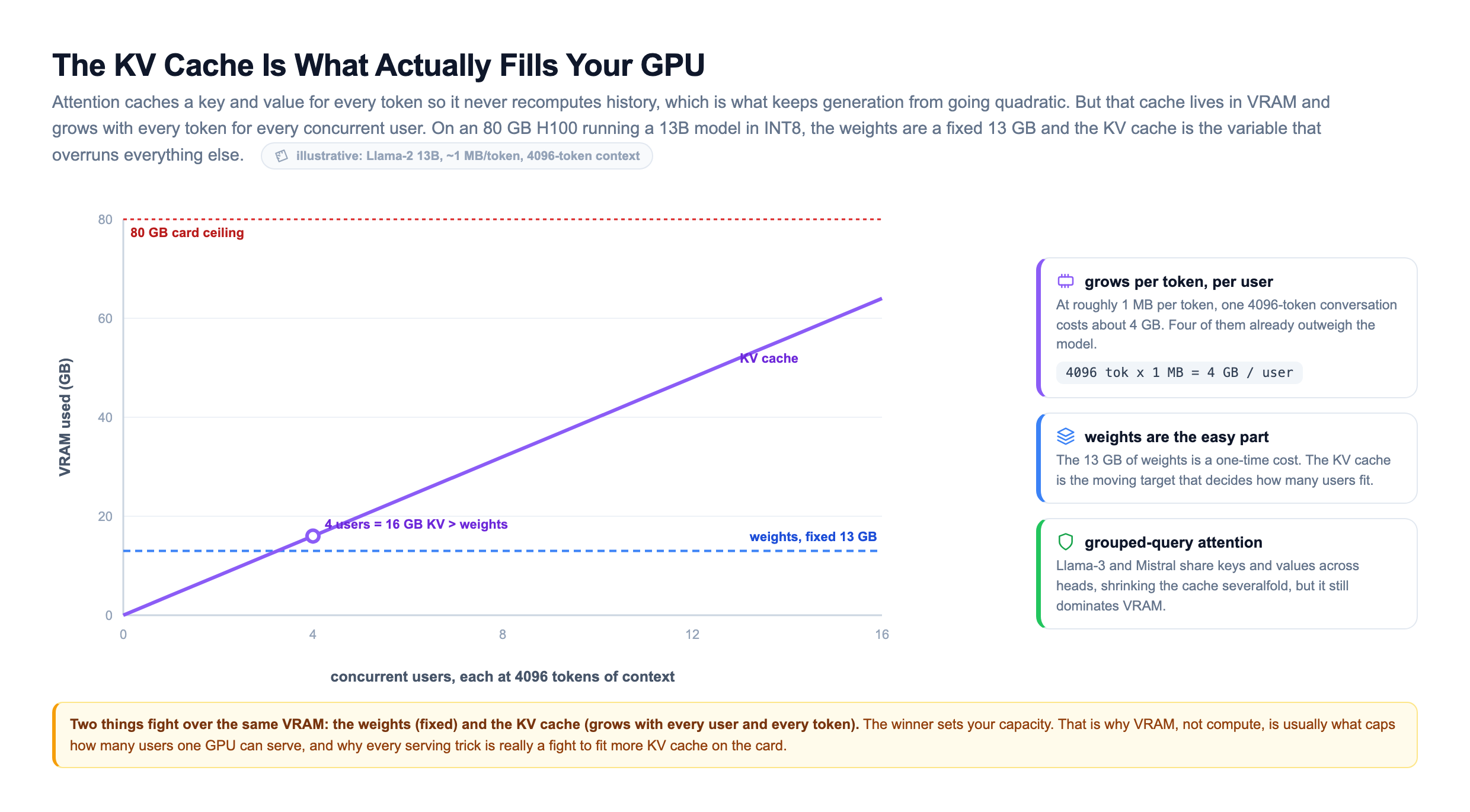
Read the crossover on that chart. The weights are a flat, one-time 13 GB. The KV cache is a rising line that passes the weights at just four concurrent users and keeps climbing toward the ceiling. Long before compute becomes the limit, you run out of room to hold everyone's cache.

Newer models attack this at the architecture level with grouped-query attention, where several attention heads share one set of keys and values instead of each keeping its own. Llama-3 and Mistral use it, and it shrinks the cache severalfold. Even then the KV cache stays the dominant pressure on VRAM, which is why VRAM, not compute, is usually what limits how many users one GPU can serve. How you manage that cache decides your throughput, and it is exactly what the next two techniques are fighting over.

Since decode reads the weights from VRAM on every step regardless of how many requests are in flight, you may as well apply those weights to many sequences in the same pass. That is batching, and it is where most of the 10 to 20x lives. But for LLMs there is a right way and a wrong way to do it, and the difference is the whole ballgame.

The wrong way is static batching: gather a group of requests, run them together, and hold the whole group until the last one finishes. The problem is that reply lengths vary by 100x. A one-line answer gets stuck waiting for a 2000-token essay in the same batch, and its slot on the GPU sits idle the entire time it waits. Utilization craters to a third of the card or worse, and you are paying full price for a mostly empty GPU.

The right way is continuous batching, popularized by vLLM. Rebuild the batch on every single decode step. The moment a sequence finishes it leaves and its slot is freed. New requests join on the very next step instead of waiting for a batch boundary. The GPU is always working on a full batch of active sequences, so the reads you were already paying for get spread across as many users as the card can hold.

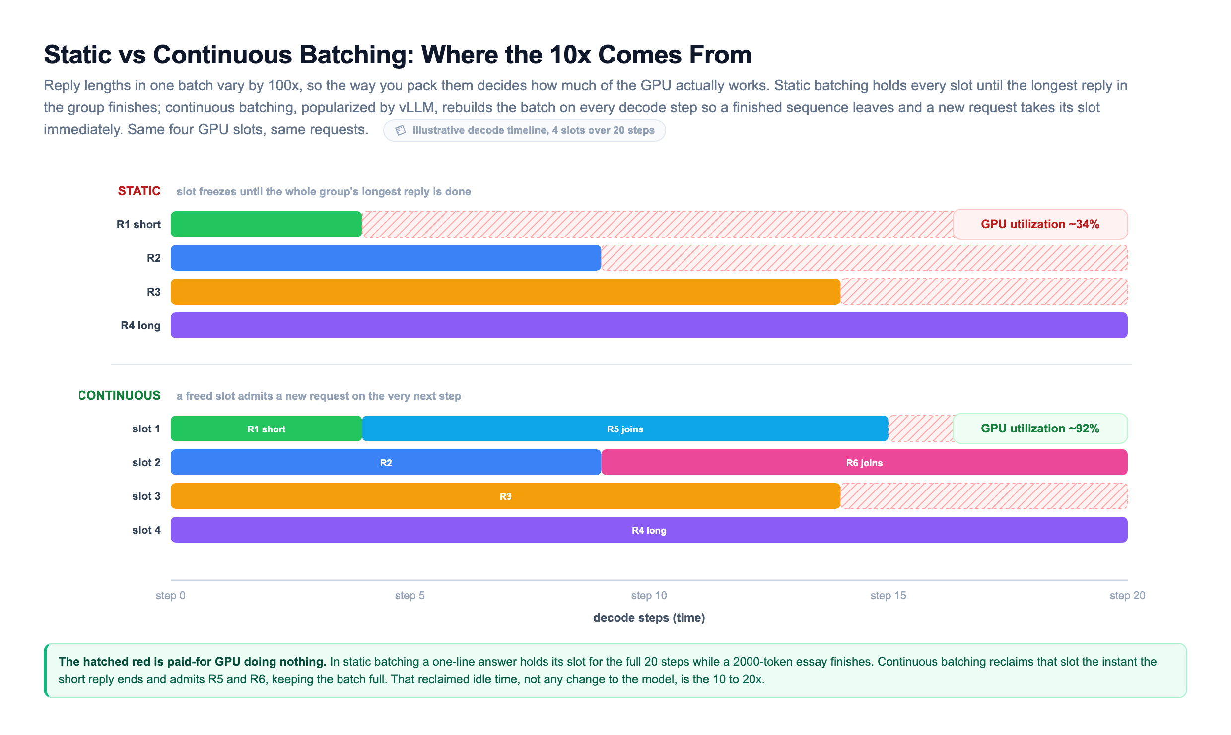
The hatched red in that figure is paid-for GPU doing nothing. Static batching leaves the short replies holding dead slots; continuous batching reclaims each slot the instant a reply ends and slides a waiting request in. That reclaimed idle time, not any change to the model, is where the throughput multiple comes from.

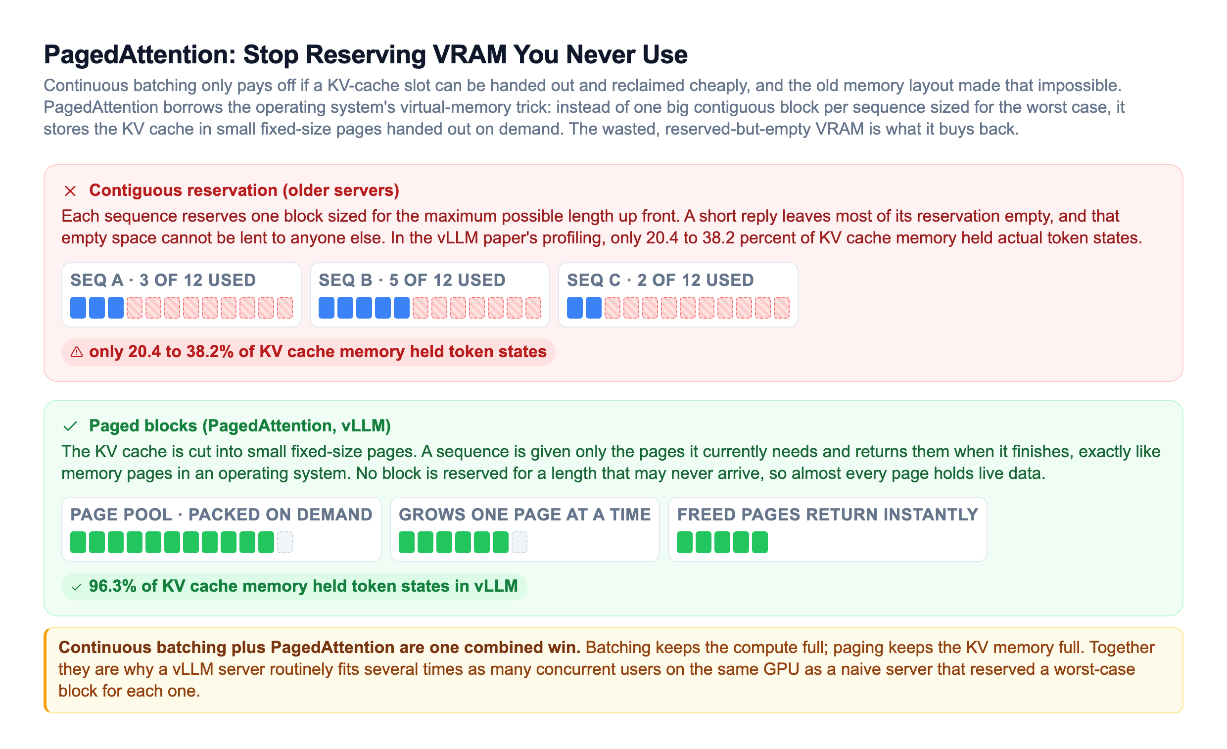
Continuous batching only works if you can hand out and reclaim KV cache slots cheaply, and that is what PagedAttention adds. Older servers stored each sequence's KV cache as one contiguous block sized for the maximum possible length. A short reply left most of its reservation empty, and that empty space could not be lent to anyone else. The vLLM paper (Kwon et al., SOSP 2023) measured how much this cost: "only 20.4% - 38.2% of the KV cache memory is used to store the actual token states in the existing systems." The rest was reserved for tokens not yet generated, or lost to internal and external fragmentation.

Decode is memory-bound, so the most direct way to speed it up is to make the weights smaller, because fewer bytes to read is less time reading. Quantization stores each weight in fewer bits. FP16 is the 16-bit baseline, INT8 halves it, and INT4 quarters it. Fewer bits means less VRAM to hold the model and fewer bytes to move every step, which is a direct decode speedup, and it also frees room for the KV cache that actually limits concurrency. Cutting a 13B model from 26 GB to 6.5 GB hands almost 20 GB back to the cache on an 80 GB card.

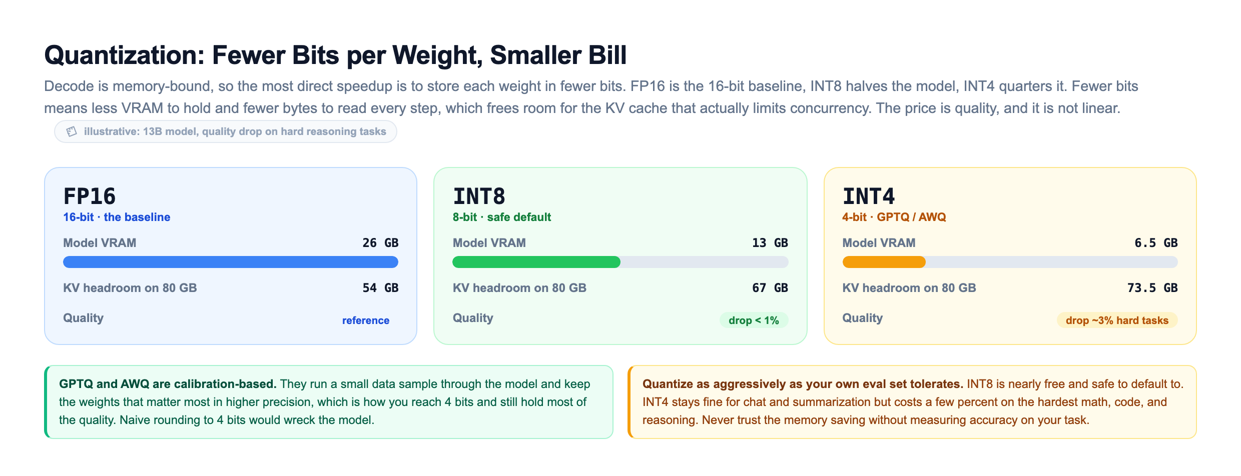
The two names you will meet most for 4-bit are GPTQ and AWQ. Both are calibration-based: they run a small sample of data through the model and choose the rounding so that the weights that matter most to the output keep their precision. That is how you drop to 4 bits and still keep most of the quality. Naive rounding to 4 bits, treating every weight as equally important, would wreck the model, and that difference is why calibration methods exist.

Serving a quantized model in vLLM is a one-line change:

# Serve a 13B model quantized to INT4 with AWQ.
# Fits in ~6.5 GB of VRAM instead of ~26 GB, leaving far more
# room for the KV cache (which is what limits concurrency).
vllm serve TheBloke/Llama-2-13B-chat-AWQ \
  --quantization awq \
  --max-model-len 4096 \
  --gpu-memory-utilization 0.90

# The endpoint is OpenAI-compatible, so clients do not change:
#   POST /v1/chat/completions  { "model": "...", "stream": true }

The trade-off is quality, and it is not linear, which is the useful part. INT8 is nearly free: usually well under a one percent drop, safe to default to for almost any workload. INT4 costs a few percent on the hardest reasoning, math, and code tasks, while staying fine for chat and summarization. The rule is simple. Quantize as aggressively as your own evaluation set will tolerate, and never trust the memory savings without measuring the accuracy on your actual task, because a benchmark number from someone else's task tells you nothing about yours.

Continuous batching and quantization make each step cheaper. Speculative decoding attacks a different weakness entirely: one slow model pass only buys you one token. What if a single pass could produce several?

The trick uses two models. A small, fast draft model guesses the next few tokens ahead. Then the big, accurate target model verifies all of those guesses in a single parallel forward pass. Verifying 4 tokens costs almost the same as generating 1, because that pass is memory-bound and you are reading the big weights exactly once either way. Every guess the target agrees with is a token you got nearly for free.

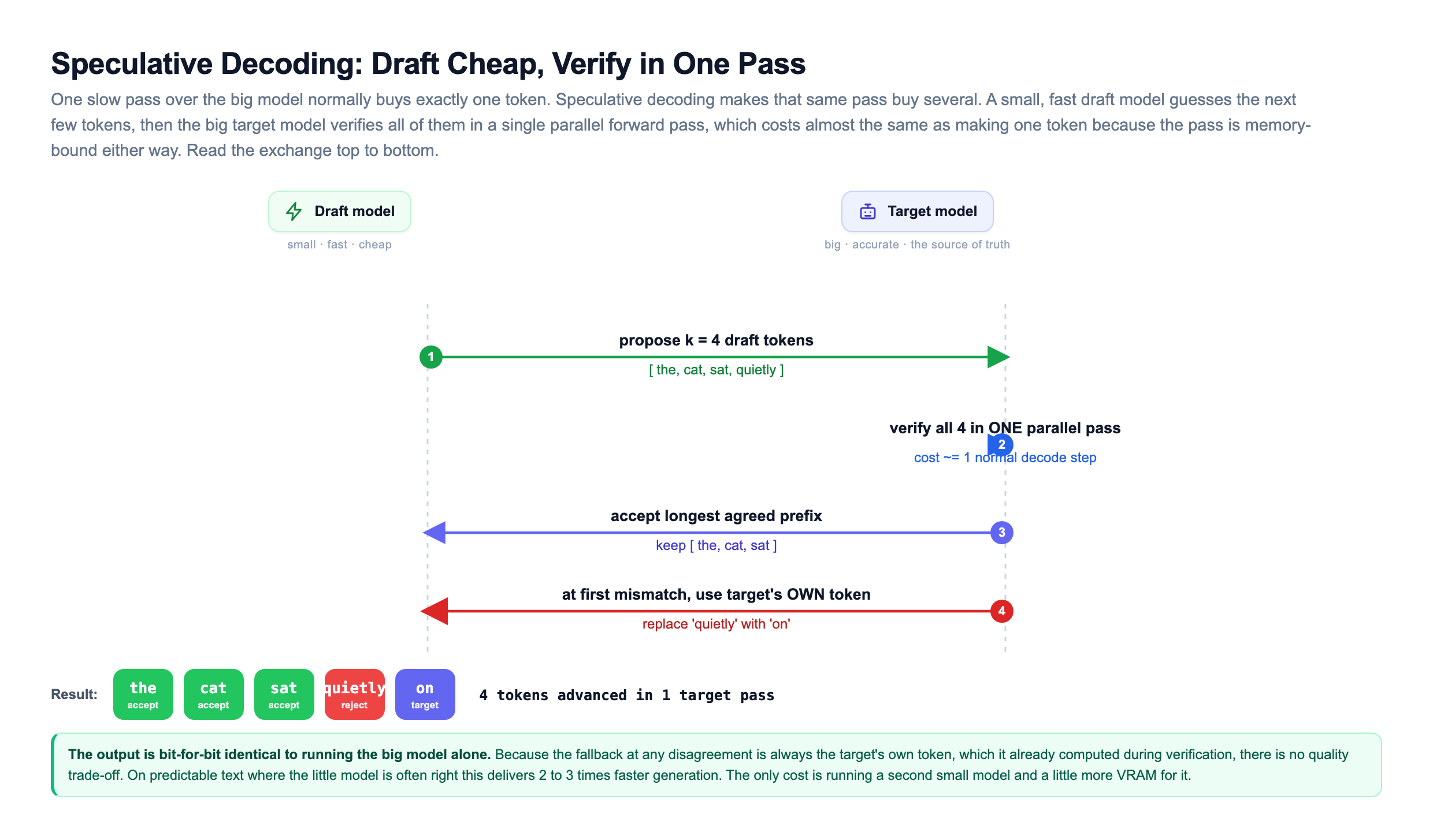
The beautiful part is correctness. At the first token where the draft and target disagree, you throw away the rest of the guesses and use the target model's own token, which it already computed during that verification pass. The output is bit-for-bit identical to running the big model alone. There is no quality trade-off whatsoever, which is rare among optimizations. On predictable text, where the little model is often right, this delivers 2 to 3 times faster generation. The only cost is running a second small model and a bit more VRAM to hold it.

Here is a runnable toy that simulates the acceptance loop. There is no real model in it, just a known target sequence and a slightly wrong draft, so you can watch how many expensive target passes it takes and confirm the output never differs from the target.

The output shows fewer target passes than tokens produced, and it confirms the generated text matches the target exactly. The toy accepts a long run and overstates the real gain, which on production text lands at 2 to 3 times, but the mechanism is the point: the expensive model runs fewer times, and it never once compromises the answer.

With the mechanisms in hand, the tuning question becomes concrete. Continuous batching lets you run many sequences at once, but how many should you run? Batch size is the one knob that trades a single user's speed for the whole fleet's efficiency, and there is no universally right setting.

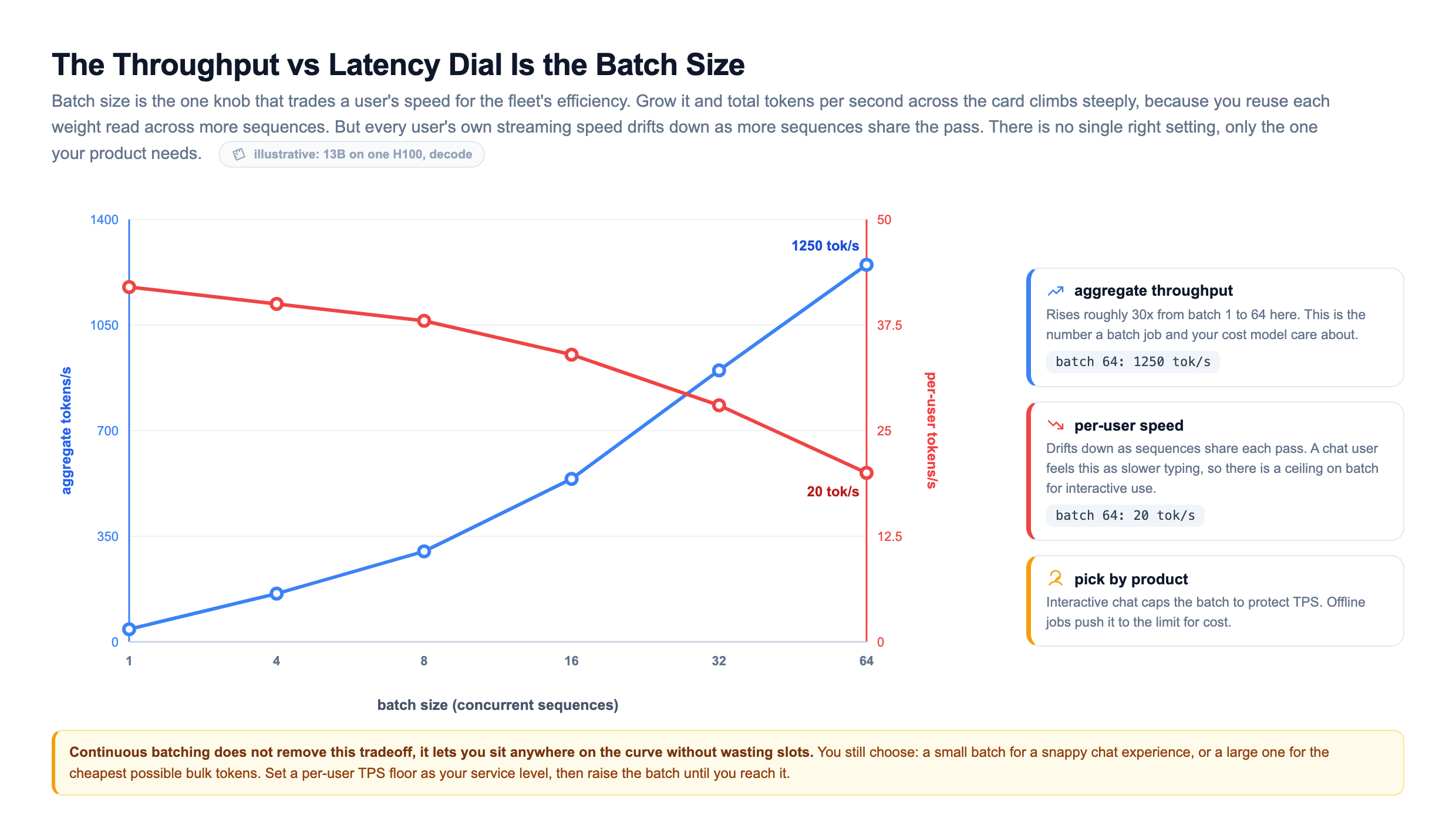
Read the two curves. As batch size grows, aggregate throughput climbs steeply, because you reuse each expensive weight read across more sequences. But per-user streaming speed drifts down, because more sequences now share each pass and each one advances a little slower. The right batch size is therefore a product decision, not a technical maximum. An interactive chat caps the batch to protect per-user TPS so the text still types out briskly. An offline job pushes the batch to the limit and does not care that any single item is slow, because it only wants the cheapest possible bulk tokens. The clean way to set it is to pick a per-user TPS floor as your service level, then raise the batch until you are about to breach it.

That efficiency is not academic, it is the entire economic case. Because the GPU rents for a fixed hourly price, cost per token is set entirely by how many tokens per second you extract from the card. Stack the levers from this lesson and the cost falls by the same factor throughput rises.

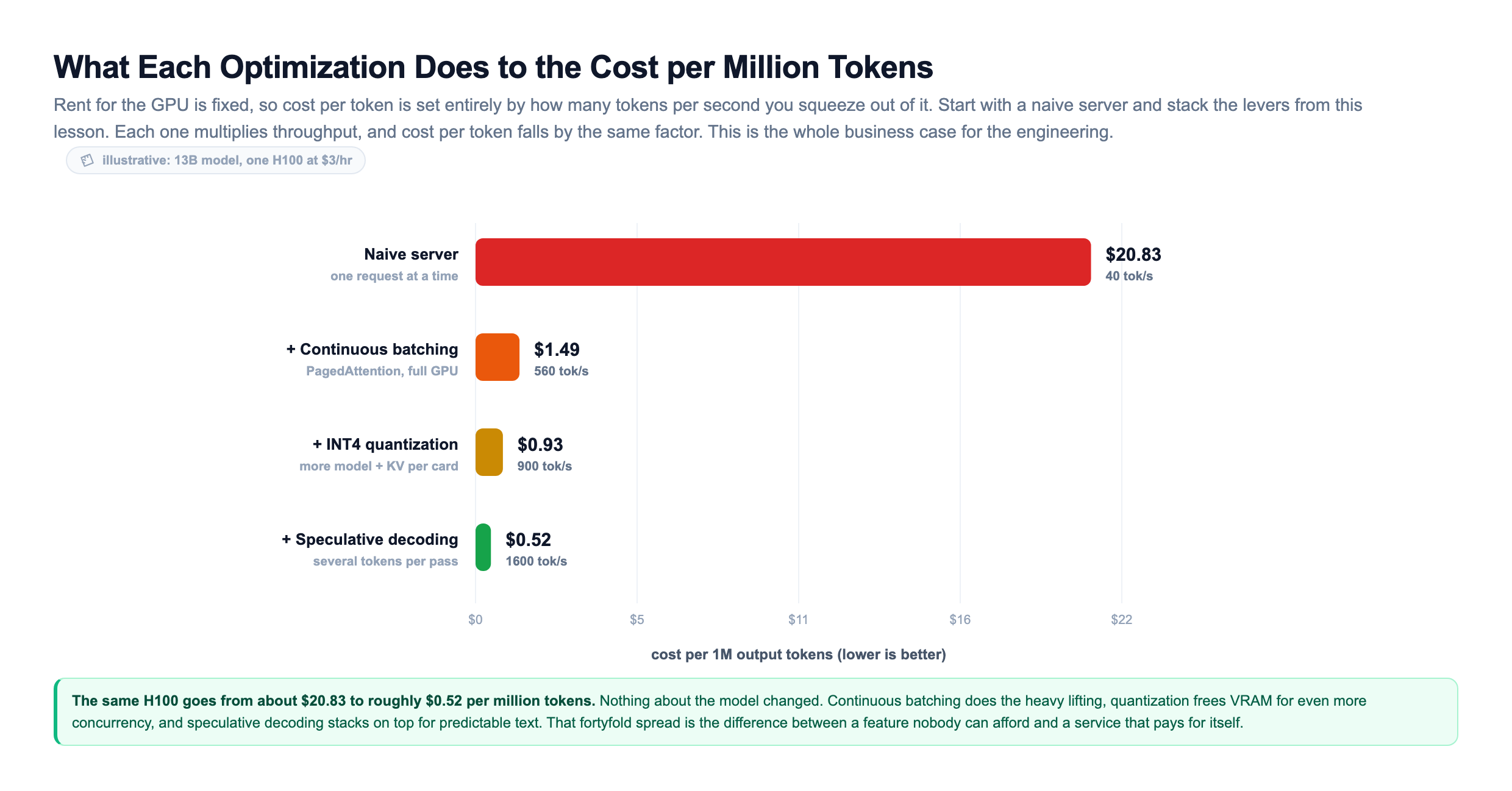
The same H100 goes from about 20 dollars per million tokens on a naive server to well under a dollar once the stack is in place. Continuous batching does the heavy lifting, quantization frees VRAM for still more concurrency, and speculative decoding stacks on top for predictable text. Nothing about the model changed. That spread is the difference between a feature nobody can afford and a service that pays for itself, and it is why serving, not modeling, is where the money is made or lost.

You almost never write this machinery yourself. You pick a serving runtime that has it built in, put it behind an orchestrator, and spend your time tuning rather than implementing. Three runtimes matter, and they overlap heavily, so the real decision is ecosystem fit and how much build complexity you will trade for the last few percent of performance.

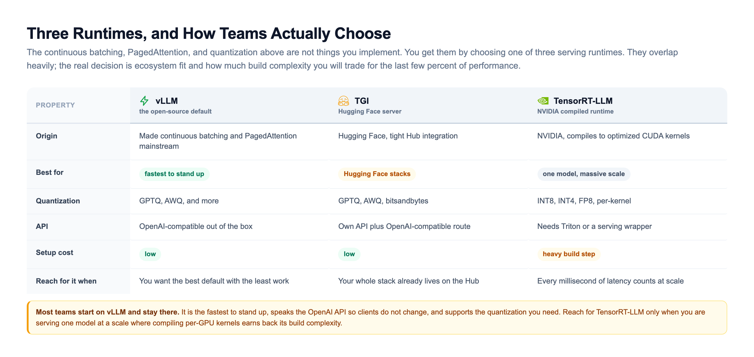
vLLM is the open-source default and the project that made continuous batching and PagedAttention mainstream. It is the fastest thing to stand up, speaks the OpenAI API out of the box so your clients do not change, and supports GPTQ and AWQ quantization. Most teams start here and never need anything else.

TGI (Text Generation Inference) is Hugging Face's server, tightly integrated with the Hub and a natural fit if your whole stack already lives in the Hugging Face ecosystem. It offers similar continuous batching and quantization support, so the choice between it and vLLM is mostly about which ecosystem you are already invested in.

TensorRT-LLM is NVIDIA's compiled runtime. It squeezes out the last drop of performance by compiling the model into optimized CUDA kernels for a specific GPU, which can beat the others on raw latency and throughput. The cost is a heavier build step and less flexibility, so teams reach for it when they are serving one model at massive scale and every millisecond counts.

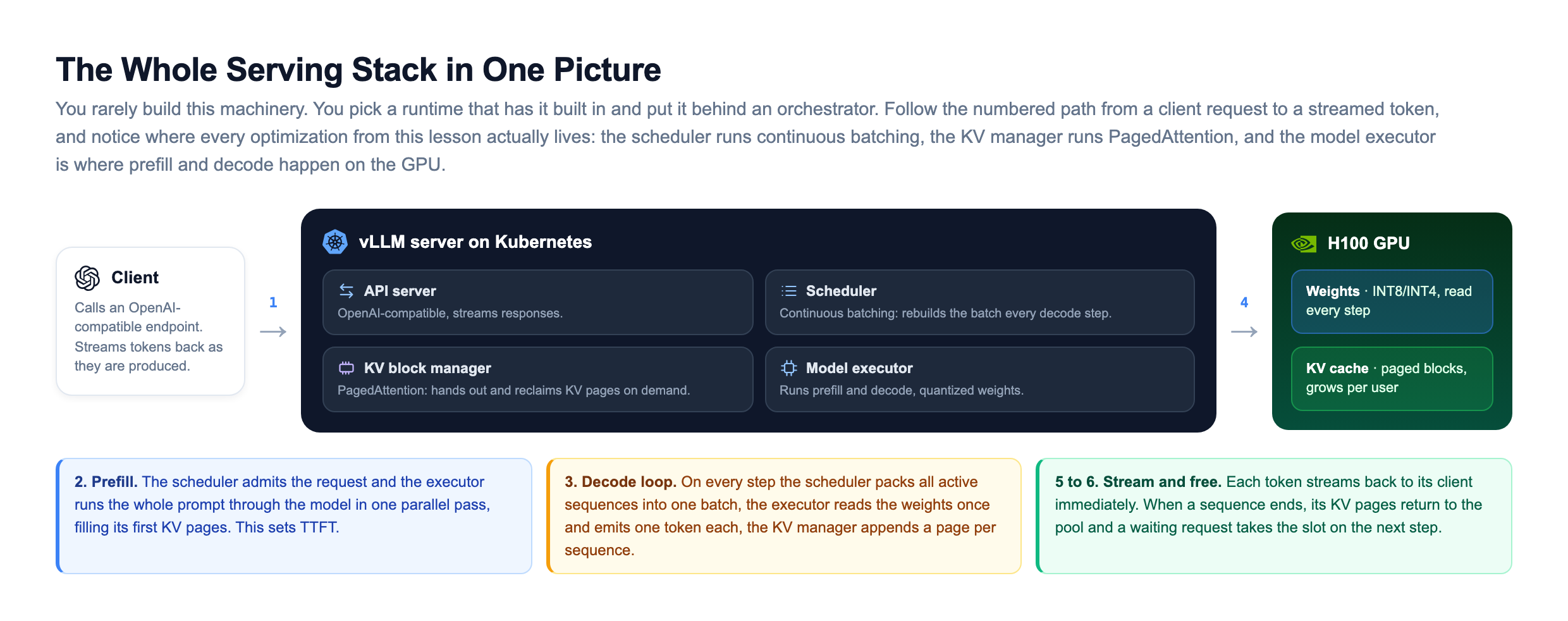
Now the whole stack in one picture. Follow the numbered path from a client request to a streamed token and notice where each optimization from this lesson lives: the scheduler is where continuous batching runs, the KV block manager is where PagedAttention runs, and the model executor is where prefill and decode happen on the quantized weights.

Here is the whole toolkit at a glance: what each lever attacks, roughly what it buys, and the honest cost. Read the last column, because none of these is free, and knowing the cost is what keeps you from cargo-culting an optimization your workload does not need.

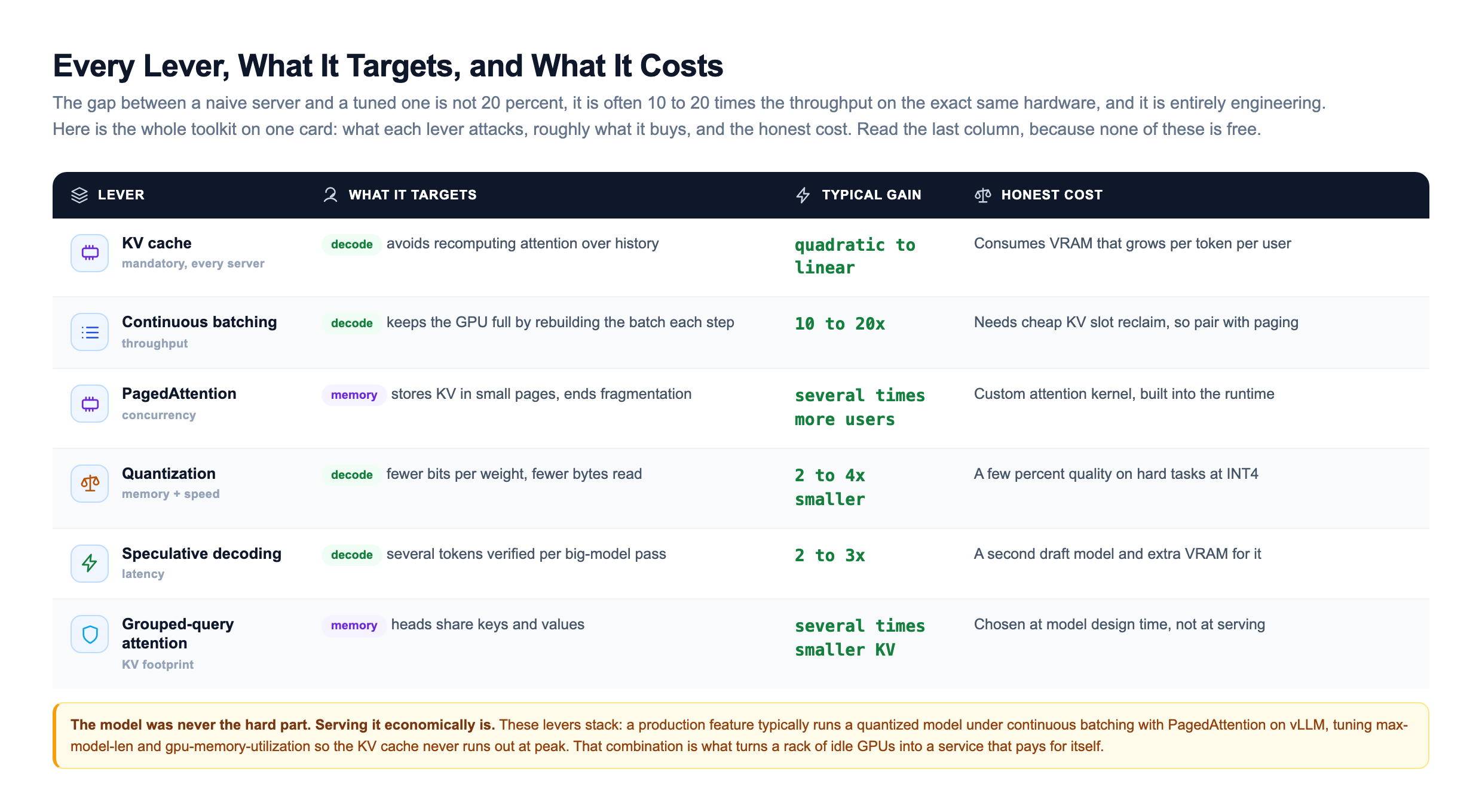
Notice the shape of the toolkit. The KV cache is not optional, every server runs it, and it is the reason concurrency is a memory question at all. Continuous batching and PagedAttention are the two that deliver the headline 10 to 20x, and they are a package because batching needs the cheap slot reclaim that paging provides. Quantization stacks a memory and speed win on top and buys back VRAM for even more concurrency. Speculative decoding is the pure latency play with no quality cost. Grouped-query attention is chosen when the model is designed, not when you serve it, but it changes how much cache pressure you inherit.

These levers stack, and a production feature usually runs several at once: a quantized model under continuous batching with PagedAttention on vLLM, with max-model-len and gpu-memory-utilization tuned so the KV cache never runs dry at peak. Reach for each one deliberately. Continuous batching and paging you want almost always. Quantization you push as far as your eval set tolerates. Speculative decoding you add when latency matters and your text is predictable enough for the draft to be right often. That deliberate stack, not any single trick, is what closes the gap between a demo and an affordable product.