Imagine you give a friend a shopping list and a recipe, and ask them to cook the same dinner on Monday and again on Tuesday. Same shop, same list, same recipe. You would expect the same dinner. But the shop has a rule you never read: at the door, one bag in every ten is taken aside at random for a quality check, and it never comes home. On Monday the missing bag held the onions. On Tuesday it held half the rice. Your friend followed the recipe exactly both times, and the two dinners taste different.

Nobody in that story made a mistake. Nobody changed the list. The difference came from a rule that was switched on by default, and that picked something at random every time. If Tuesday's dinner is worse, you cannot find out why by reading the recipe, because the recipe did not change.

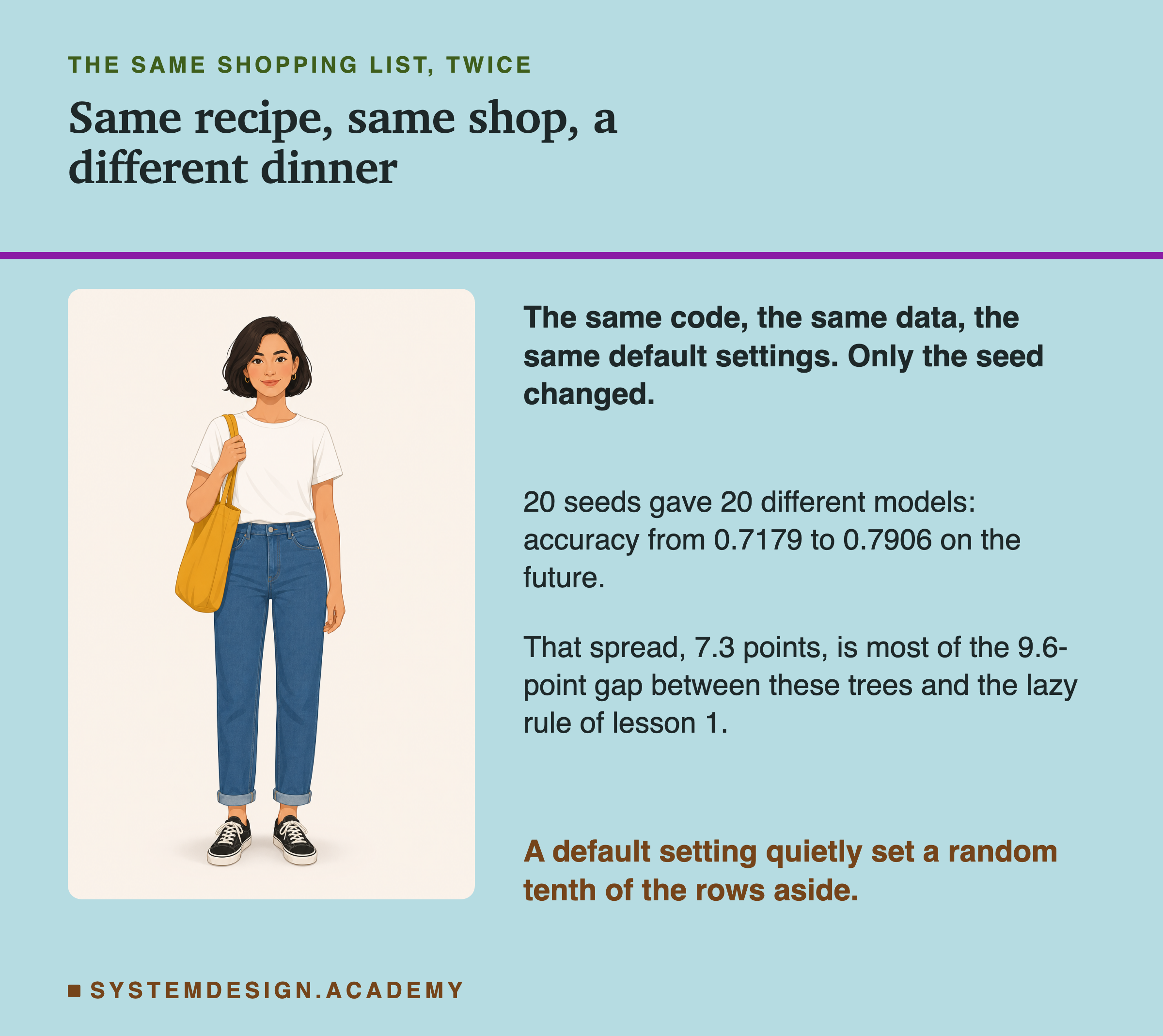
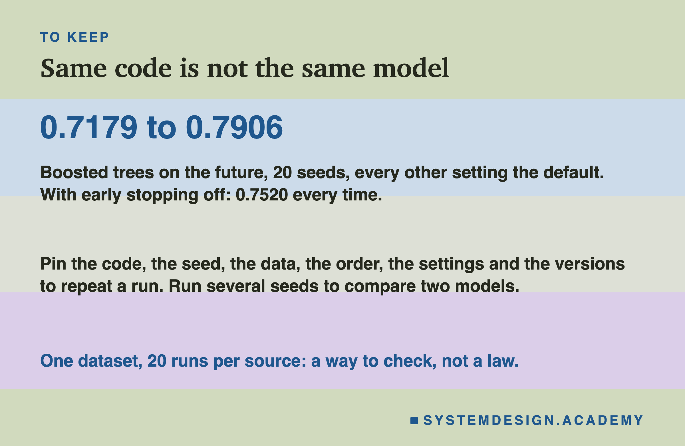
This lesson is about the same thing in a computer program that learns from examples. I trained one program 20 times with the same code on the same data and got 20 different programs out. Their scores on the future ran from 0.7179 to 0.7906. The reason was one setting I never wrote, left at its default value, which set aside a random tenth of the examples every time. The rest of the lesson finds that setting, measures what it does, and shows what to write down so that a run can be repeated exactly, and why, even then, one run is not enough to say that one program is better than another.

The lesson before this one, start with the dumbest model, trained boosted trees on electricity prices and scored them against simple rules that learn nothing. The trees scored 0.7527 on the future. A rule that just repeats the previous half-hour's answer scored 0.8484. Every model in that lesson ran once with seed 0, except a follow-up that ran the trees with the previous label as an extra input (trees plus lag) with 20 seeds. That lesson ended with a question: if I train the same model twice, on the same data, with the same code, do I get the same model?

The pipelines lesson, training pipelines and orchestration, has a slide called "Reproducibility: Freeze All Three Inputs". It explains, in words, that a run can only be replayed if its data, its code and its environment were frozen and recorded. I will not repeat it here. This lesson measures it, and adds a fourth input that slide does not name: the random choices a training run makes, including the ones hidden inside default settings that nobody chose.

In the life of a model, this is still the training step. It matters for every step after it. If a shipped model misbehaves, you need to rebuild it to debug it. If an auditor asks how a decision was made, you need to show the exact model. If a new model is worse, you need to go back to the old one. And if you want to know whether a change helped, you need to compare two runs that differ only in that change. All four need a run that can be repeated.

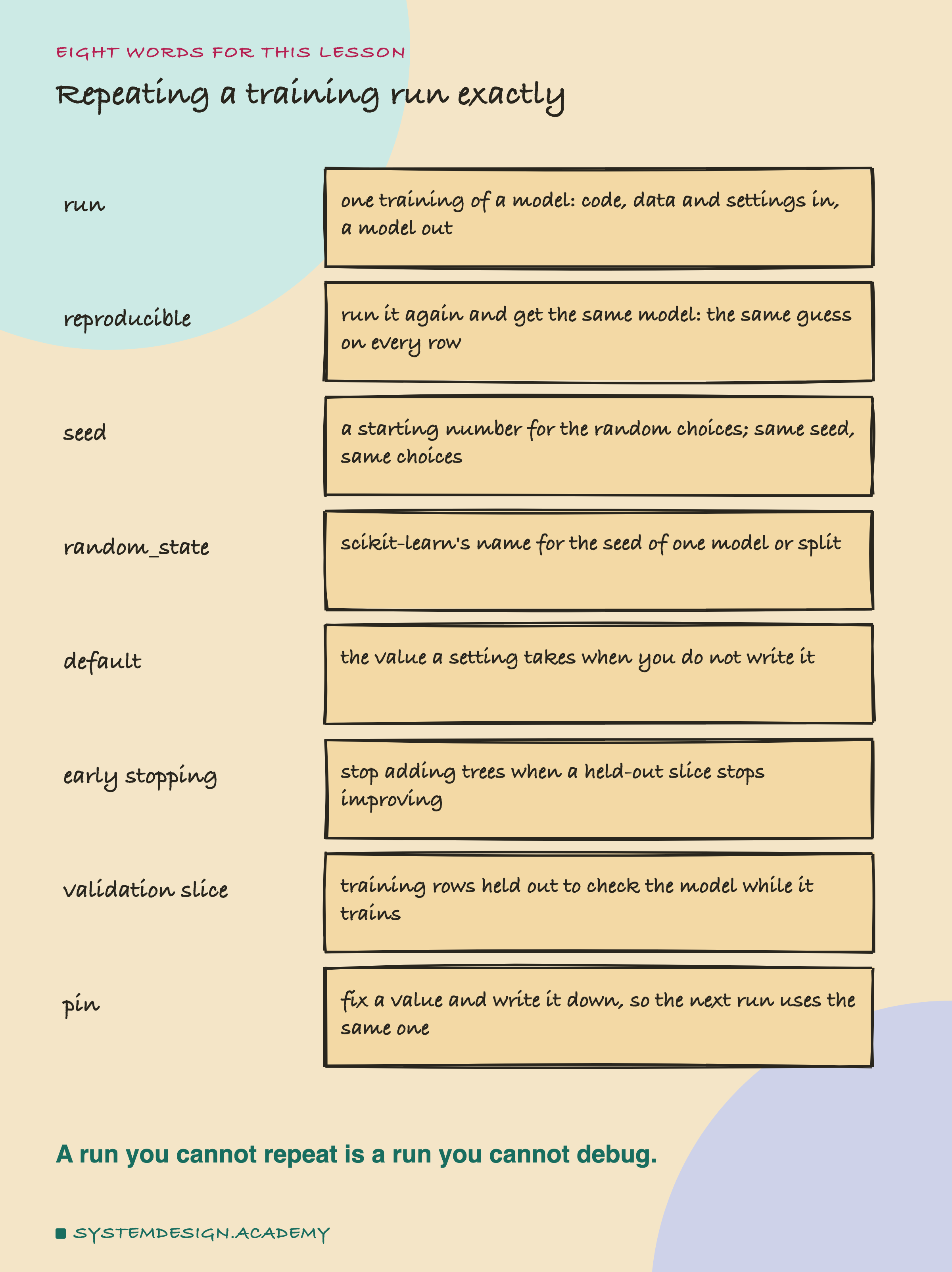
A run is one training of a model: code, data and settings go in, a trained model comes out. A run is reproducible if you can run it again and get the same model, meaning the same guess on every row, not just a similar score.

Many training methods make random choices on purpose: which rows to look at, in which order, which to hold back. A computer makes these choices with a random number generator, which is not truly random. It produces a fixed sequence of numbers from a starting number called the seed. The same seed gives the same sequence, and so the same choices. In scikit-learn, the Python library used in this chapter, the seed of a model or a split is a setting called random_state.

A default is the value a setting takes when you do not write it. Early stopping is a rule for boosted trees: keep adding trees only while a held-out slice of the training rows keeps getting better, and stop when it stops improving. That held-out slice is the validation slice. To pin something is to fix its value and write it down, so the next run uses the same value.

Before the numbers, here is why a team should care, in the order the lifecycle meets it.

Debugging. A model in production starts making strange guesses. The first thing anyone does is rebuild it and look inside. If the rebuild gives a different model, you are no longer looking at the model your users met. You are looking at a different one that was trained the same way.

Audits. Some models make decisions that people can challenge: a loan, a price, an alert. When someone asks why, you need to show the exact model that decided, and show that anyone following your record would get the same one.

Rollback. A new model goes live and does worse, so you go back to the old one. If the old one's file was kept, that is easy. If only its code was kept, you must train it again, and you will only get the old model back if the run repeats.

Comparing models. This is the one people forget. A team changes one thing, say a setting or a new input column, trains again, and sees the score go up. Did the change help? Only if the two runs differed in that change and nothing else. If the training itself moves the score by several points from run to run, a single before-and-after pair tells you nothing. This lesson measures how much it moves here.

I wrote the design at the top of the lab file, repro_lab.py, before I ran it. The dated record is the chapter plan, CHAPTER-PLAN.md (2026-09-29, "REPRO LAB (batch 2) designed before running").

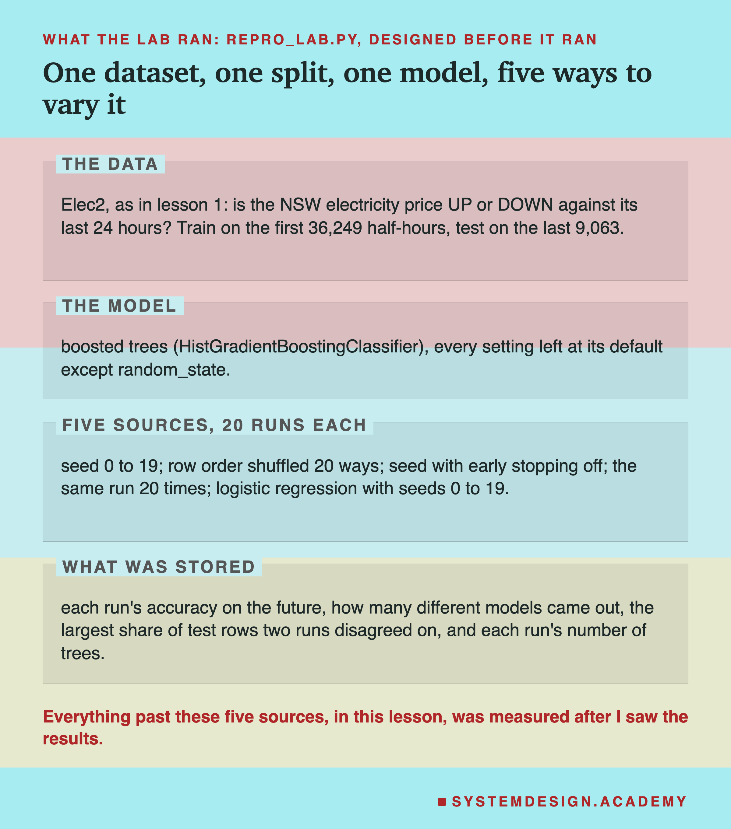
The data is Elec2 again, as in lesson 1: 45,312 half-hours of the New South Wales electricity market from 1996 to 1998, in time order. Each row asks: is the price UP or DOWN compared with its average over the last 24 hours? The split is forward in time: train on the first 36,249 rows, test on the last 9,063, which are the future from the model's point of view. Accuracy is the share of test rows where the guess was right.

The model is scikit-learn's HistGradientBoostingClassifier, which I call boosted trees. It builds up to 100 small decision trees, one after another, each one correcting the mistakes of the ones before. Every setting was left at its default except random_state.

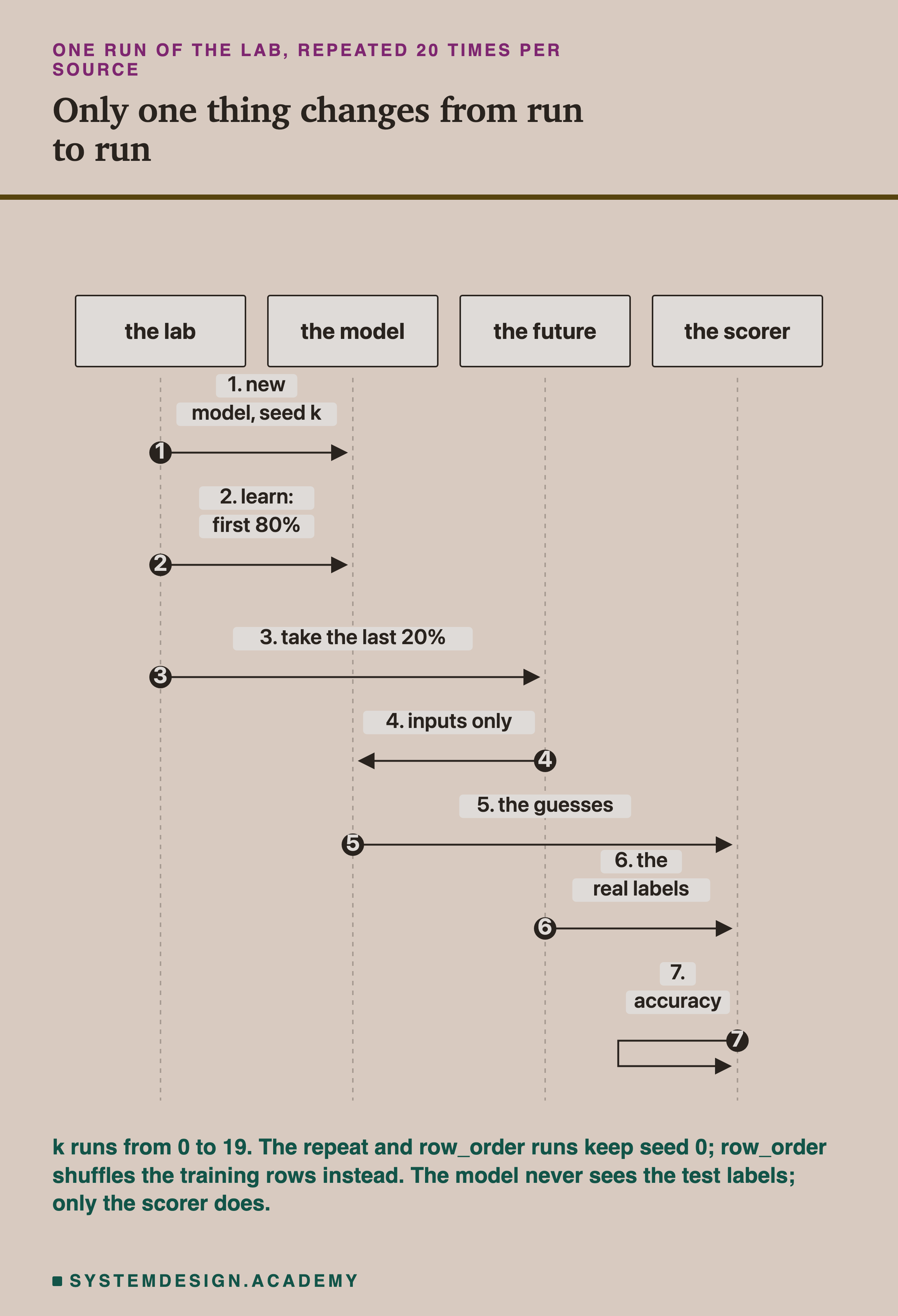
Five sources of variation, each run 20 times. seed: random_state from 0 to 19, rows in their original order. row_order: random_state fixed at 0, training rows shuffled 20 different ways. : seeds 0 to 19 again, with early stopping switched off. : seed 0, rows in order, the same run 20 times; it should never change. : a simpler model, , which adds up a weight for each input and turns the total into a chance of UP; it ran with seeds 0 to 19, and its default method has no random steps, so it was expected not to change.

Here is the headline, straight from the lab's stored file, results/repro.json.

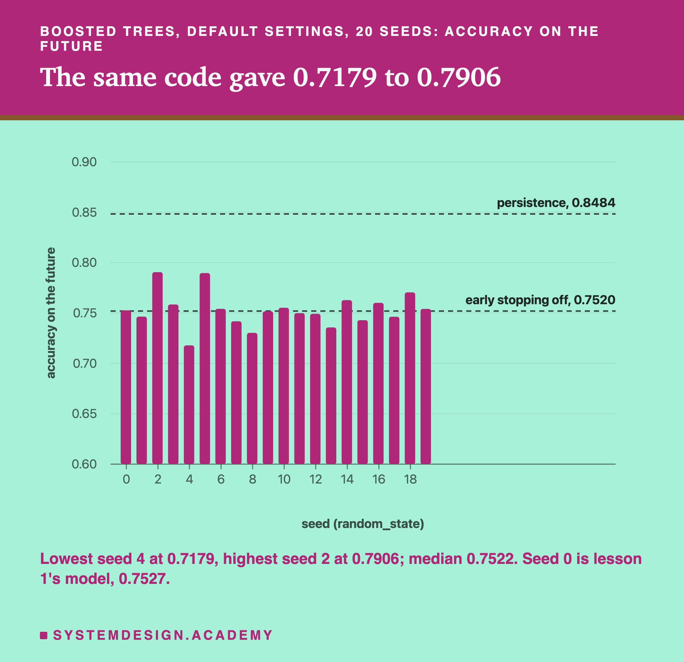
With the seed as the only change, the 20 runs scored from 0.7179 (seed 4) to 0.7906 (seed 2). That is a spread of 0.0727, or 7.3 percentage points, which I will just call points. The median, the middle value when the 20 scores are put in order, was 0.7522, and the mean 0.7530. Every one of the 20 runs gave a different model. Seed 0 is lesson 1's model, 0.7527, so lesson 1 happened to land in the middle.

The scores are only part of it. Two of these 20 models disagreed on up to 19.7% of the test rows: for about one test row in five, the answer depended on which seed was used, a number nobody chose for any reason.

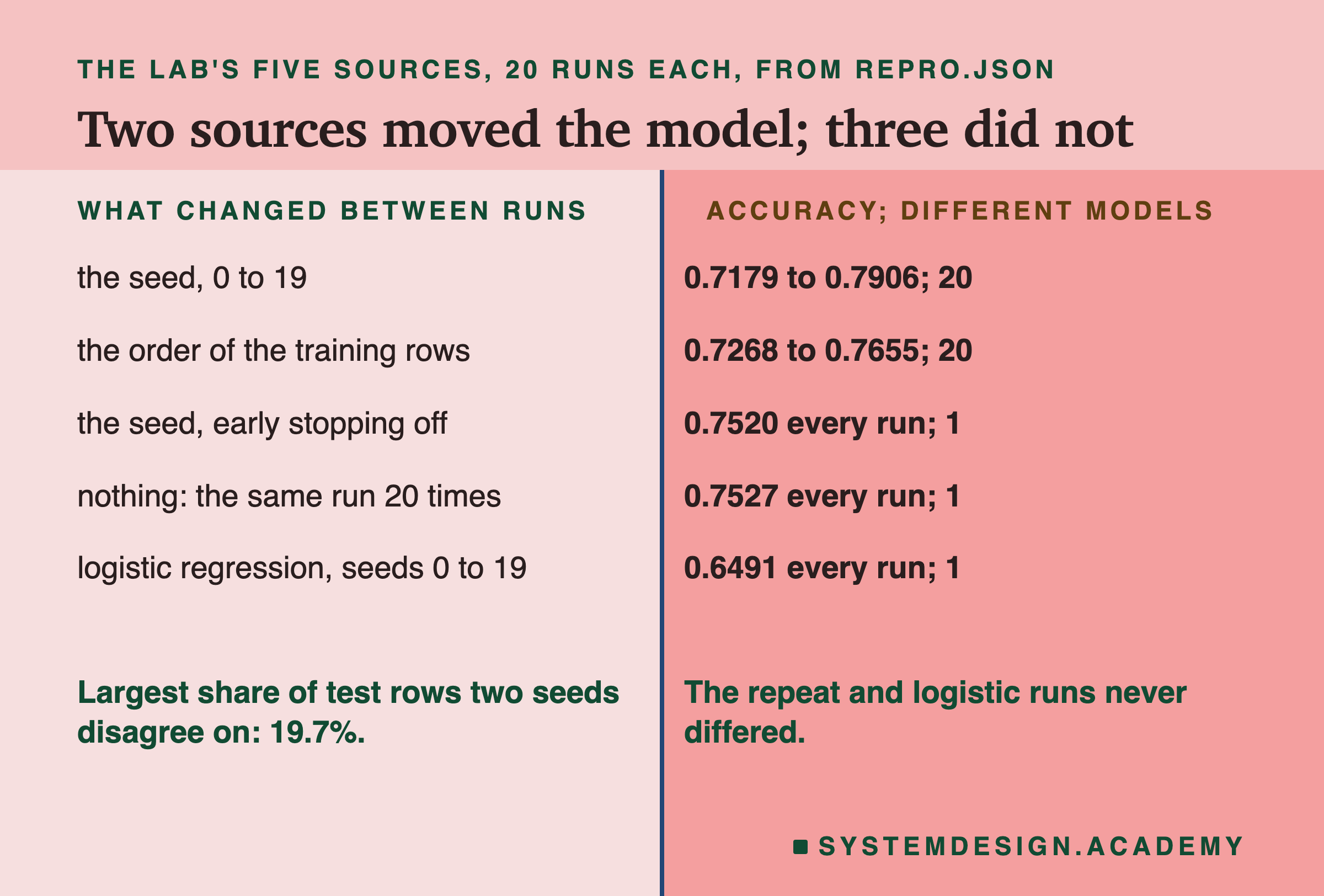
The other four sources tell you where to look. Shuffling the training rows with the seed held at 0 also gave 20 different models, from 0.7268 to 0.7655. Running the same seed on the same rows 20 times gave one model, 0.7527 every time, so the computer itself is not adding noise here. Logistic regression gave one model, 0.6491, whatever its seed. And the boosted trees with early stopping switched off gave one model, 0.7520, for every one of the 20 seeds. So the seed only mattered while early stopping was on.

A spread only means something next to the decisions it could change. Lesson 1 compared the trees with simple rules, and its follow-up also ran the trees plus lag with 20 seeds. Here are both sets of 20 seeds, next to logistic regression and persistence, on one chart.

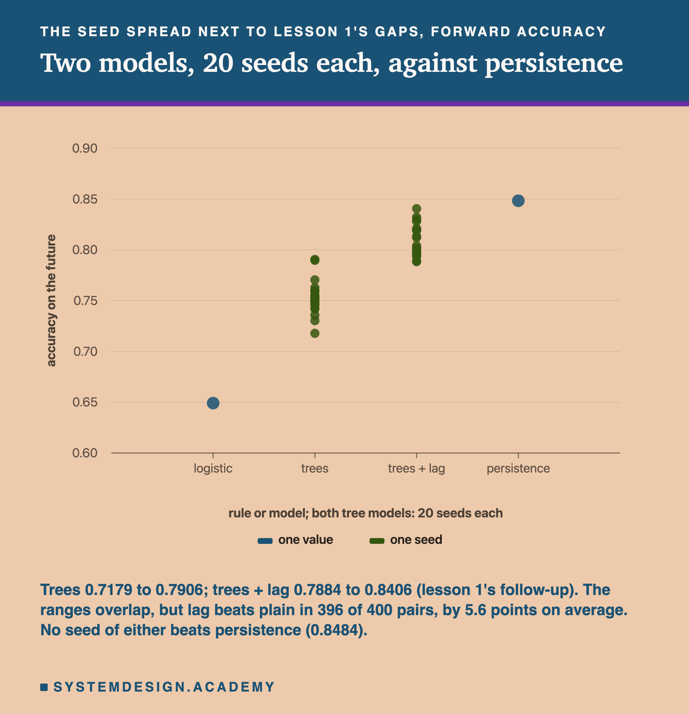
The gap in lesson 1 between the trees (0.7527) and persistence, the rule that repeats the previous half-hour (0.8484), was 9.6 points. The spread from the seed alone is 7.3 points, three quarters of that gap. Even so, every one of the 20 seeds stayed below persistence and above logistic regression, so this ranking does not depend on the seed.

The trees plus lag show what a closer call looks like. With seed 0, lesson 1 measured a gain of 6.7 points over the plain trees (0.8193 against 0.7527). Its follow-up ran the trees plus lag with 20 seeds: they scored from 0.7884 to 0.8406, with a mean of 0.8091, and none of the 20 beat persistence. The two ranges overlap: the best plain seed, 0.7906, is above the worst lag seed, 0.7884. So a single run of each could, with unlucky seeds, have put the plain trees ahead. Paired every way, 20 lag seeds against 20 plain seeds, the lag model won 396 of the 400 pairs, and its mean gain was 5.6 points, not the 6.7 that seed 0 showed. The gain is real on this data; its size, measured once, was a little flattering.

Why does the seed matter only while early stopping is on? I read the scikit-learn source code installed on my machine (version 1.9.1) to find out, then measured what I read. Everything on this slide was added after I saw the results.

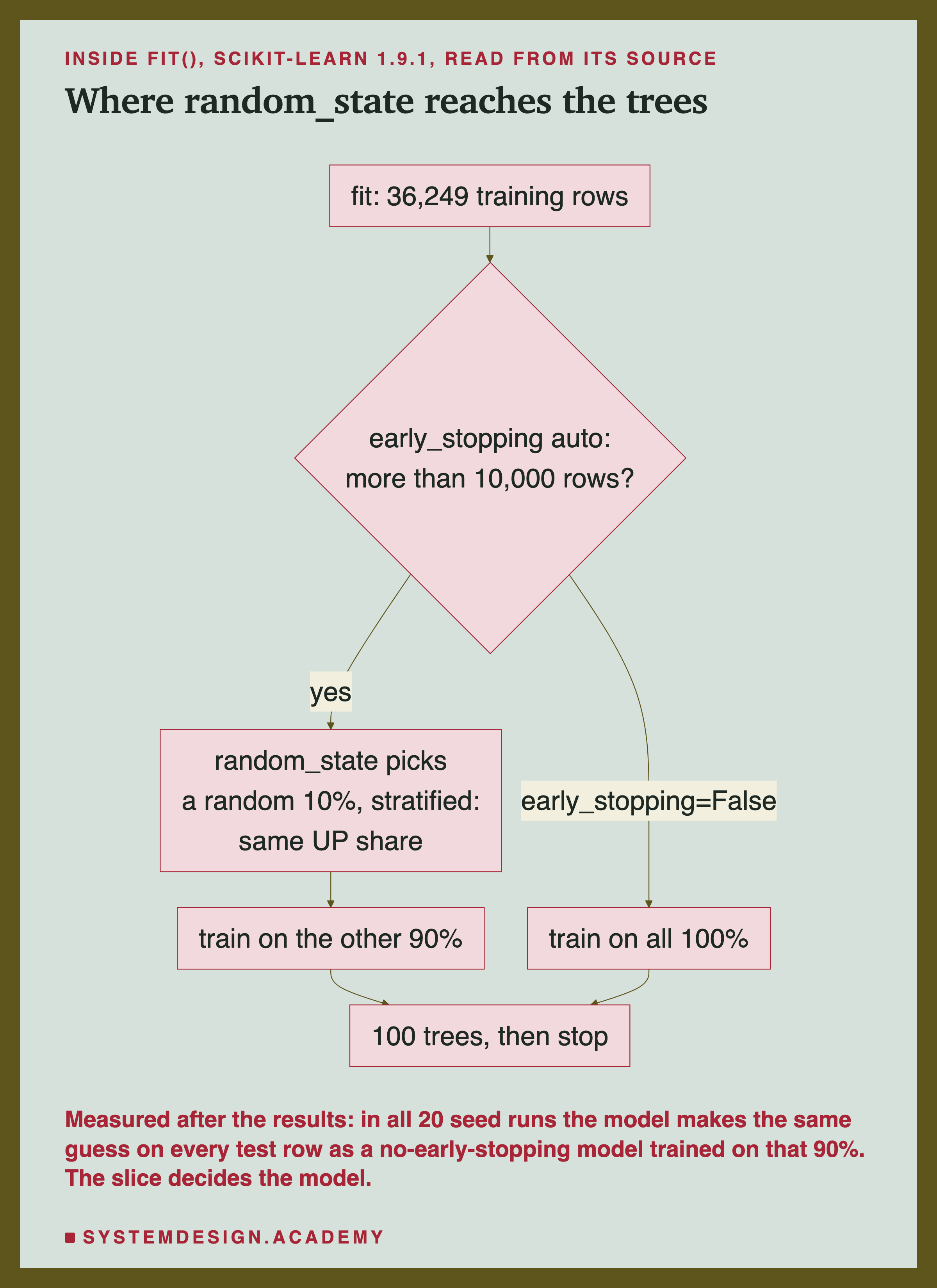
The documentation for early_stopping says: "If 'auto', early stopping is enabled if the sample size is larger than 10000 or if X_val and y_val are passed to fit." The default is 'auto'. In the code, the line is self.do_early_stopping_ = n_samples > 10_000. Our training set has 36,249 rows, so early stopping was on, and nobody asked for it.

The documentation for validation_fraction, default 0.1, says: "Proportion (or absolute size) of training data to set aside as validation data for early stopping." And for random_state: "Pseudo-random number generator to control the subsampling in the binning process, and the train/validation data split if early stopping is enabled." In the code, fit draws a number from random_state and passes it to scikit-learn's own train_test_split, with stratify=y. Stratified means the slice keeps the same share of UP and DOWN as the training rows. Two other uses of the seed did not apply here. The subsampling for binning only starts above 200,000 rows (subsample=int(2e5) in the binning code). And the same seed also drives feature subsampling, choosing a random subset of the inputs at each split, but only when the setting is below 1; its default is 1, so that was off too.

The row_order source kept the seed at 0 and shuffled the training rows instead. It also gave 20 different models. Is the order of the rows a second, separate source of randomness?

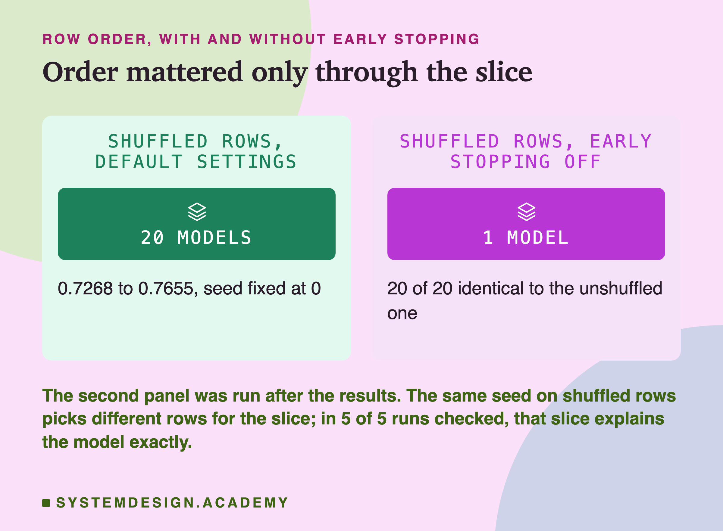
Here it was not. The split that makes the slice picks positions: "the rows at these places in the list". Shuffle the list and the same seed picks different rows. To test that, the report trained the same 20 shuffles with early stopping off, which the lab had not done. All 20 made exactly the same guesses as the unshuffled model. Then, for the first five shuffles, it rebuilt the slice from the shuffled list and trained a no-early-stopping model on the rows left behind: all five matched their default runs exactly. So, for these trees, the order of the rows mattered only because it changed which rows the slice took. That is measured on these trees; other methods, such as ones that learn from rows in small batches, can depend on the order directly.

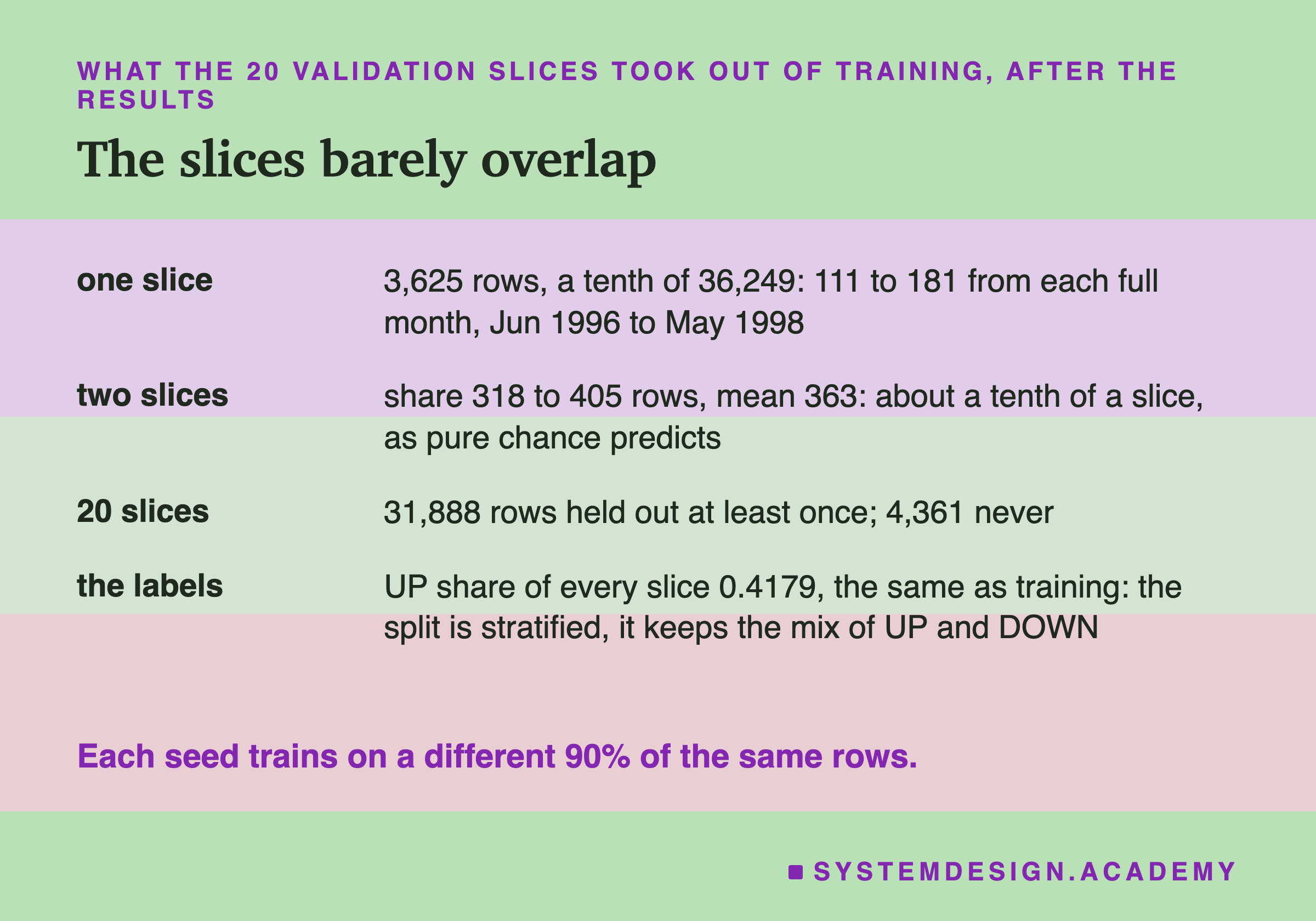
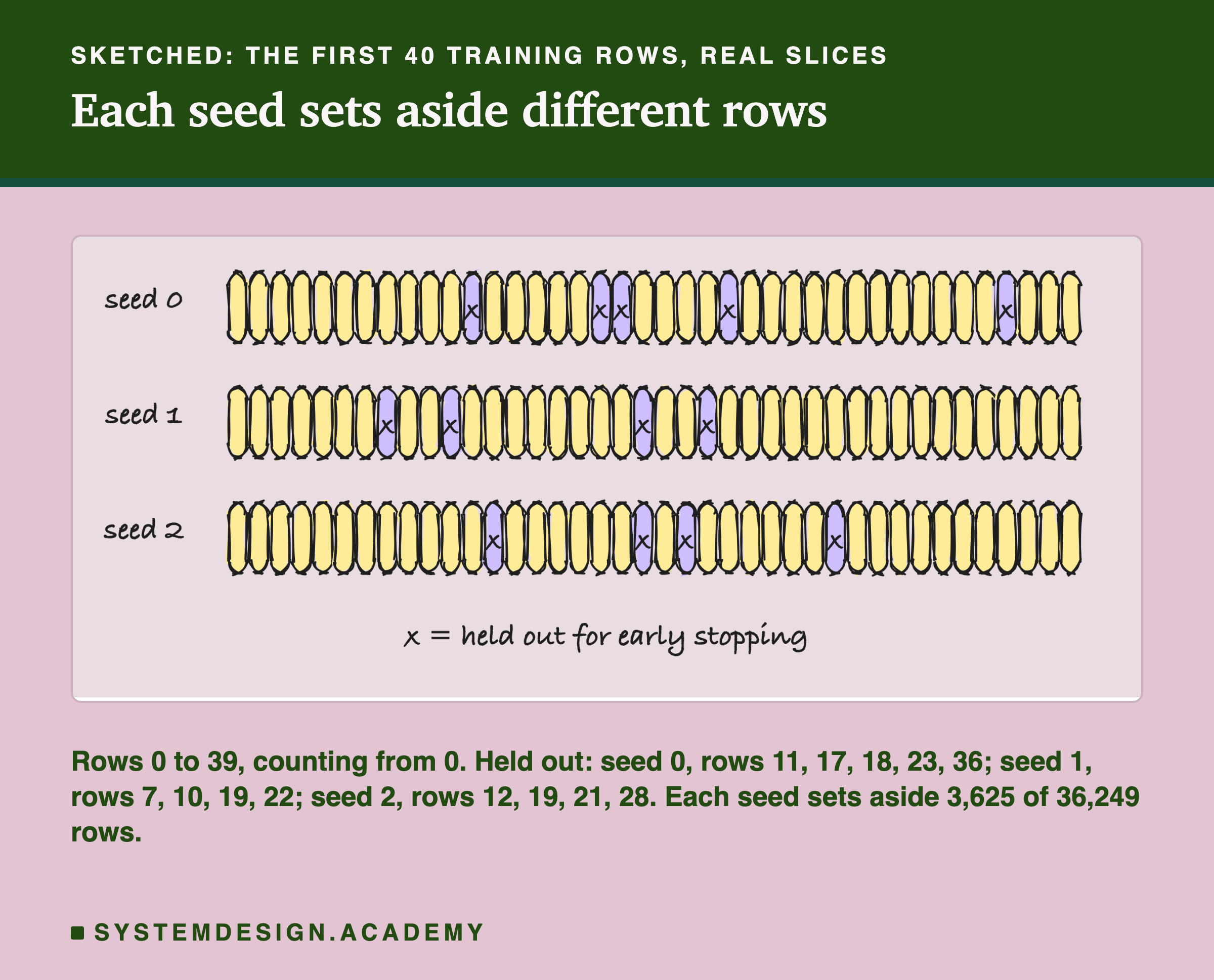
How different are the slices? Each takes rows from all through the training period, and two slices share only about 363 rows, a tenth of each slice, which is what two random draws would share. Across 20 seeds most training rows were left out at least once. Because the split is stratified, every slice had the same share of UP rows as training, so the seeds did not differ in how many UP rows they saw, only in which ones.

Why would a different tenth of the rows change the model so much? What follows is general reasoning about how boosted trees work, not something this lab measured. Each tree asks yes-or-no questions such as "is the NSW price above a certain value?", and it picks those values, the cut points, from the training rows it is given. Take away a different tenth and some cut points move a little. The next tree is built to fix the mistakes of the trees before it, so a small change in the first tree changes what the second one learns, and so on for 100 trees. The final models can then disagree on the rows that sit near a cut point, and the next slide shows where they did.

The lab stored accuracies, not guesses. To see which test rows the seeds disagree on, the report trained the 20 seed models again and stopped unless every accuracy matched repro.json to twelve decimal places. They all matched. Everything on this slide was added after the results.

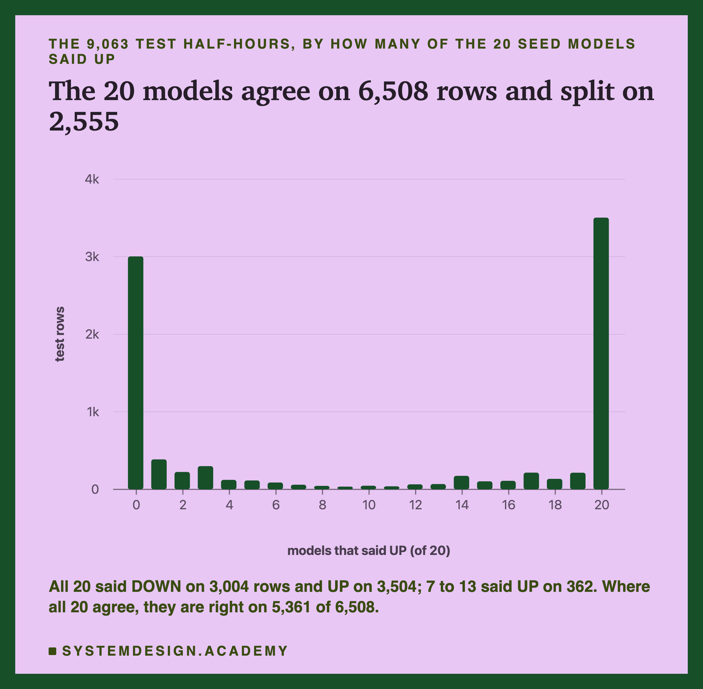
All 20 models gave the same answer on 6,508 of the 9,063 test rows, and they were right on 5,361 of those. All 20 said DOWN on 3,004 rows and UP on 3,504. On the other 2,555 rows, at least one model said something different. On only 362 of them were the models close to evenly divided, with 7 to 13 of the 20 saying UP; on the rest, 6 models or fewer went against the others.

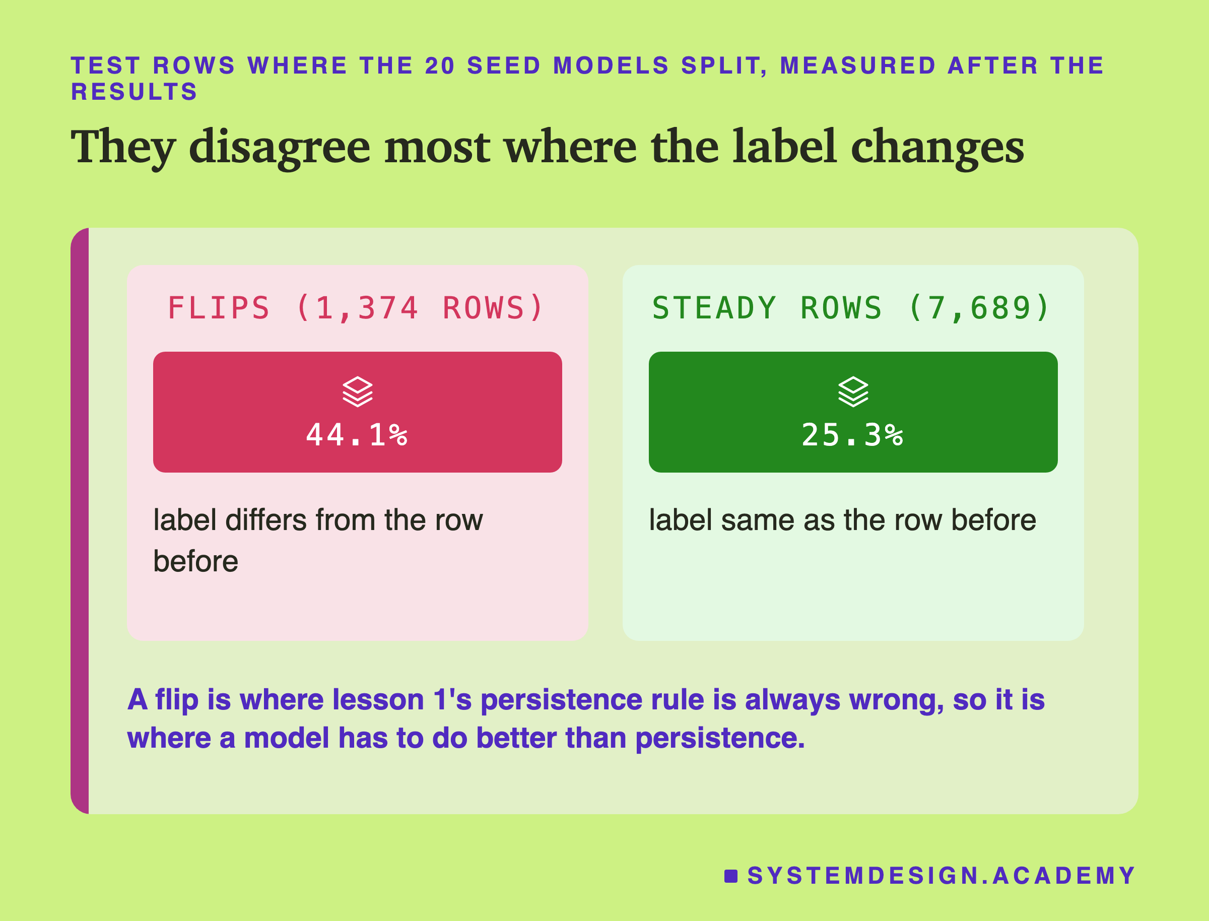
A flip is a row whose label is not the same as the row before it. Lesson 1 found that persistence is wrong on exactly those rows, so the flips are the only rows where a model can gain on persistence. The seeds split on 44.1% of the flips and on 25.3% of the steady rows. The rows that matter most for beating persistence are the rows where the seed matters most.

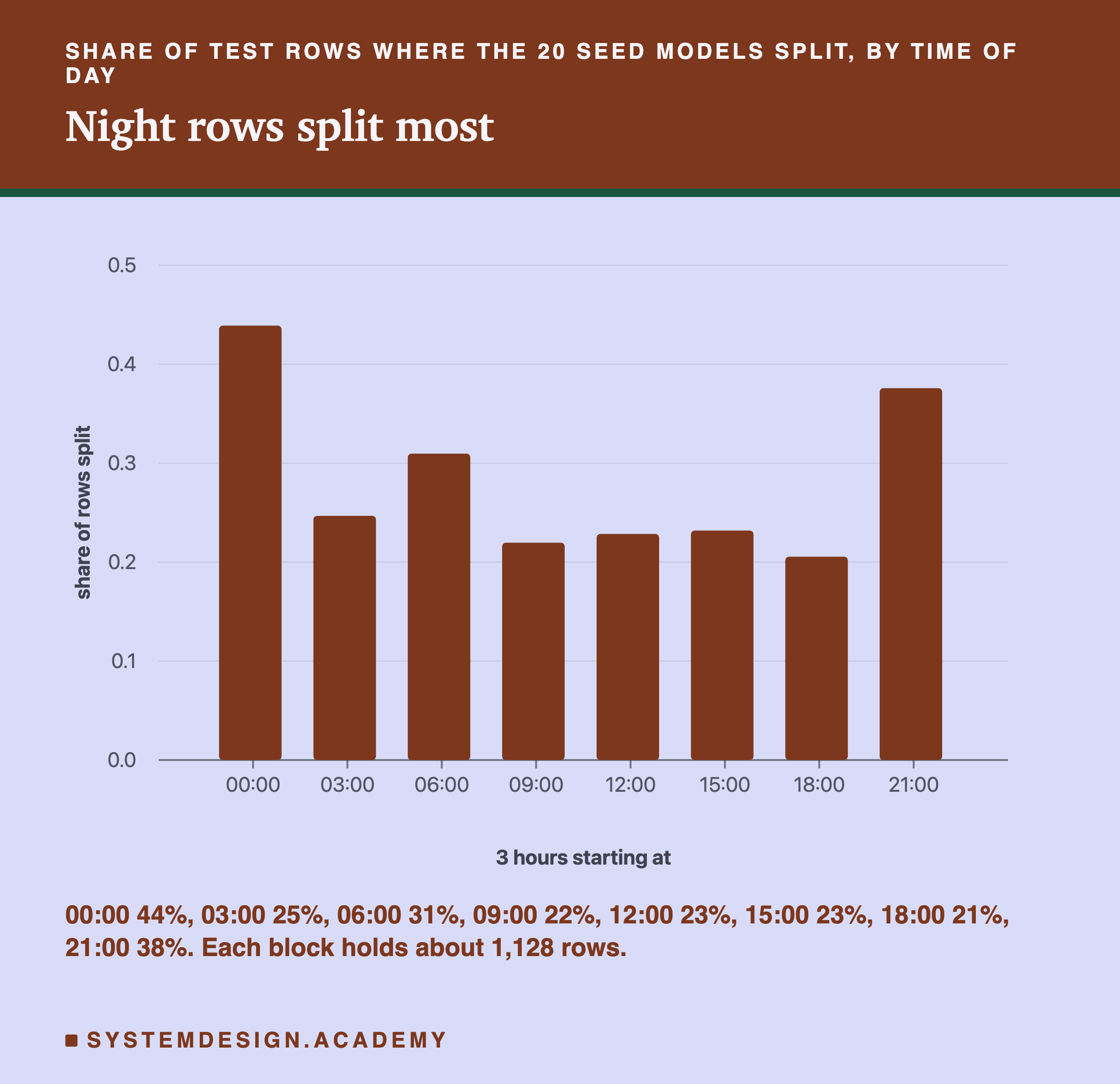
By time of day, the seeds split most on the rows from midnight to 03:00 (44% of rows) and from 21:00 to midnight (38%), and least from 09:00 to 21:00, between 21% and 23%. I do not know why. I checked the two obvious reasons in the report and neither fits. It is not the flips: the block with the most flips, 06:00 to 09:00 (25.2% of its rows), splits less than midnight to 03:00, which has 19.2%. And it is not how much the price moves: 03:00 to 06:00 has the smallest average change from one half-hour to the next, yet only 25% of its rows split.

Lesson 1 found that the trees broke down in July 1998: seed 0 said UP on about nine rows in ten when fewer than half were UP. Here is the same test, month by month, for all 20 seeds.

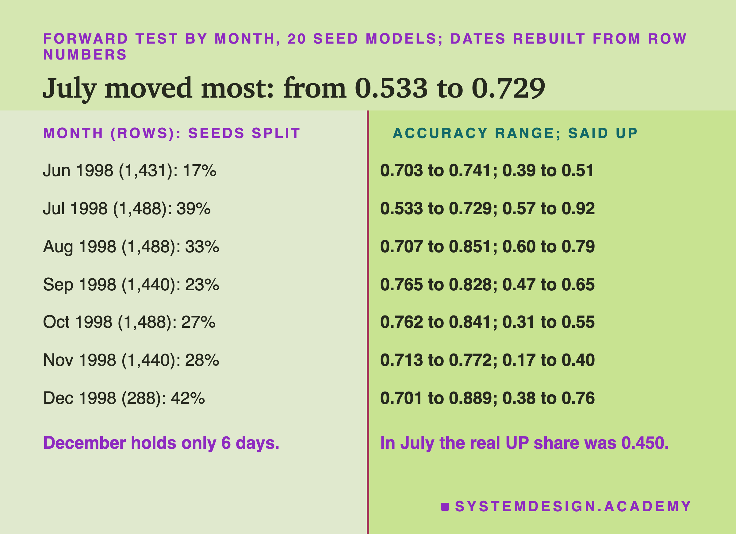
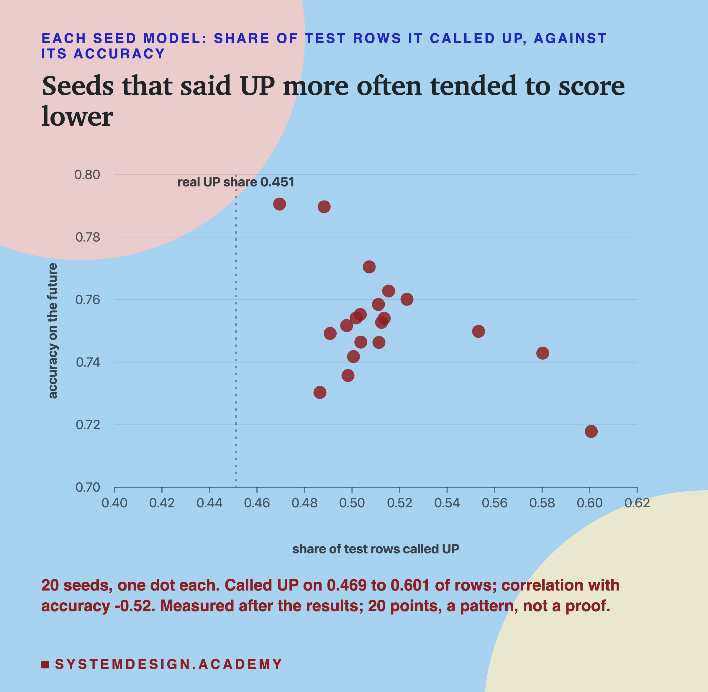
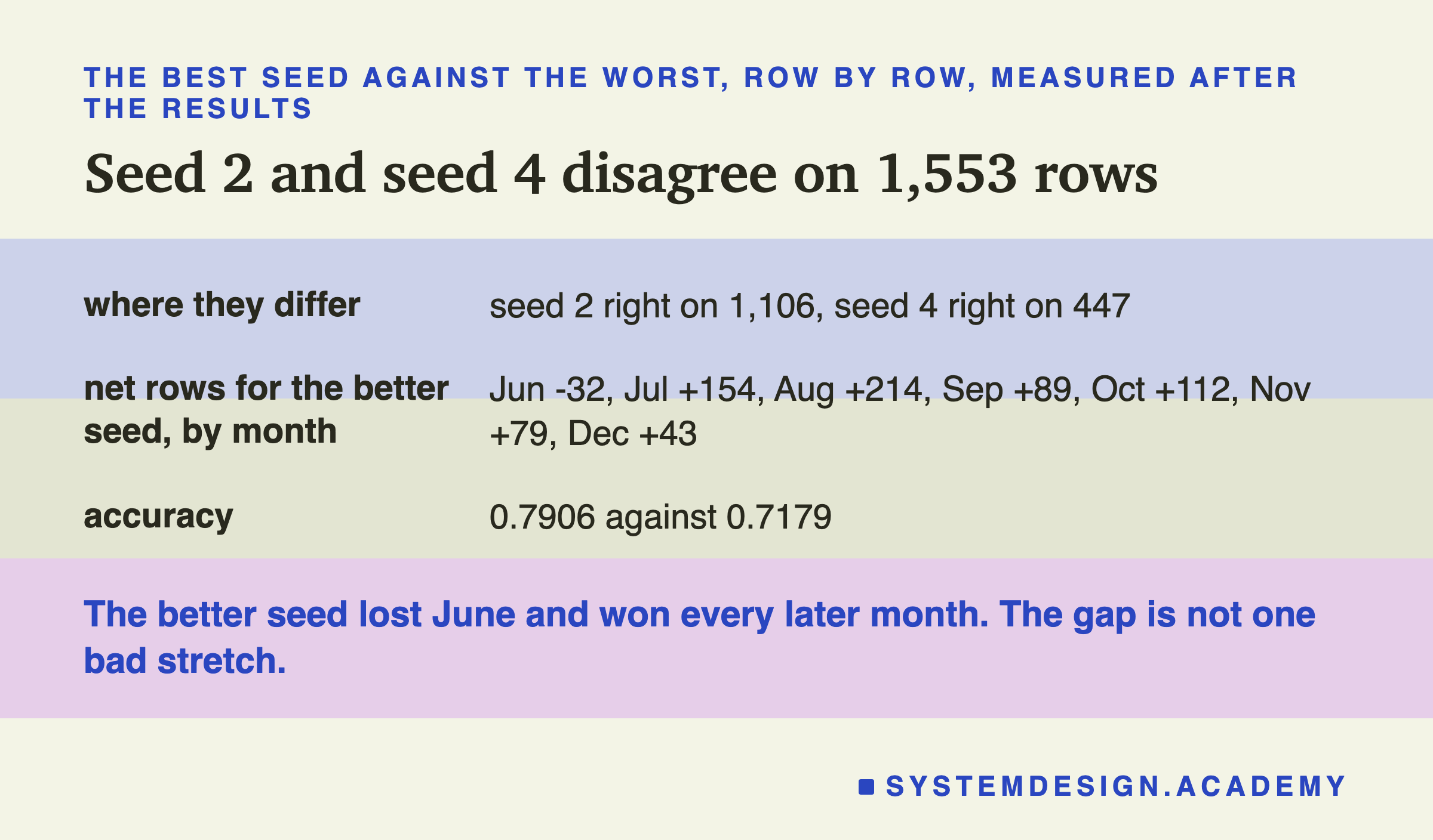
July is where the seed mattered most. Across the 20 seeds, July's accuracy ran from 0.533, only a little better than guessing at random, to 0.729. Seed 0, lesson 1's model, scored 0.553 in July, the 7th lowest of the 20, so another seed would have told a milder story about that month. But the failure itself is not the seed: every seed called UP on more July rows than were UP, 0.571 of rows or more against 0.450. December varied a lot too, but it holds only six days.

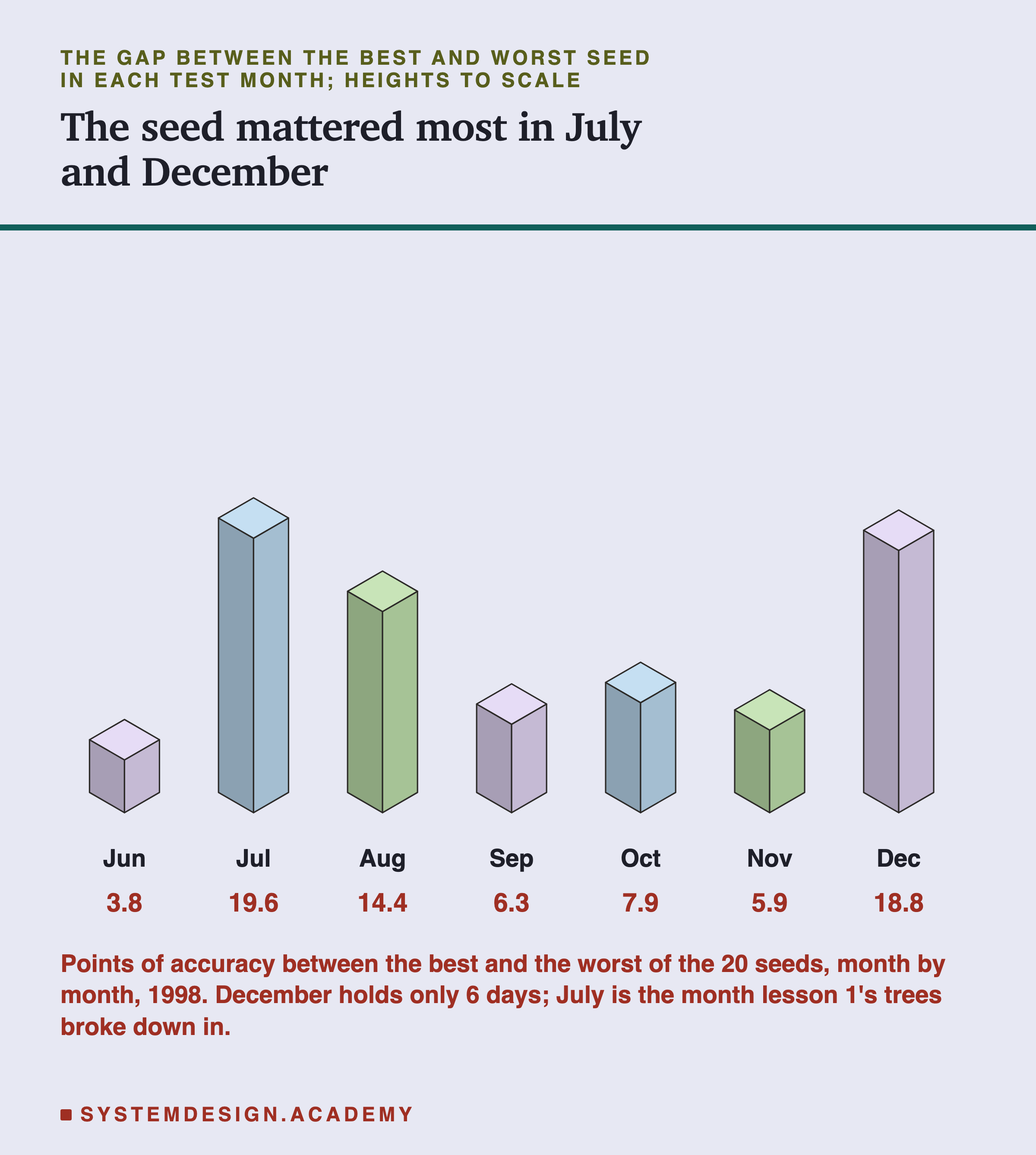
What lesson 1 measured about July: its average price was well above the training average, 0.0726 against 0.0556. Those numbers are on the dataset's own scale: Elec2 stores every price as a number between 0 and 1, not in dollars. One possible reason for the seed mattering most there, and it is a guess: when prices are unusual, the trees are guessing beyond what they learned, and small differences in the training rows push those guesses in different directions. In June, the first month of the test and the closest to training, the best and worst seed were only 3.8 points apart.

Now the lifecycle question. A team trains a model twice, changes one thing in between, and compares the two scores. How often would the seed alone fool them?

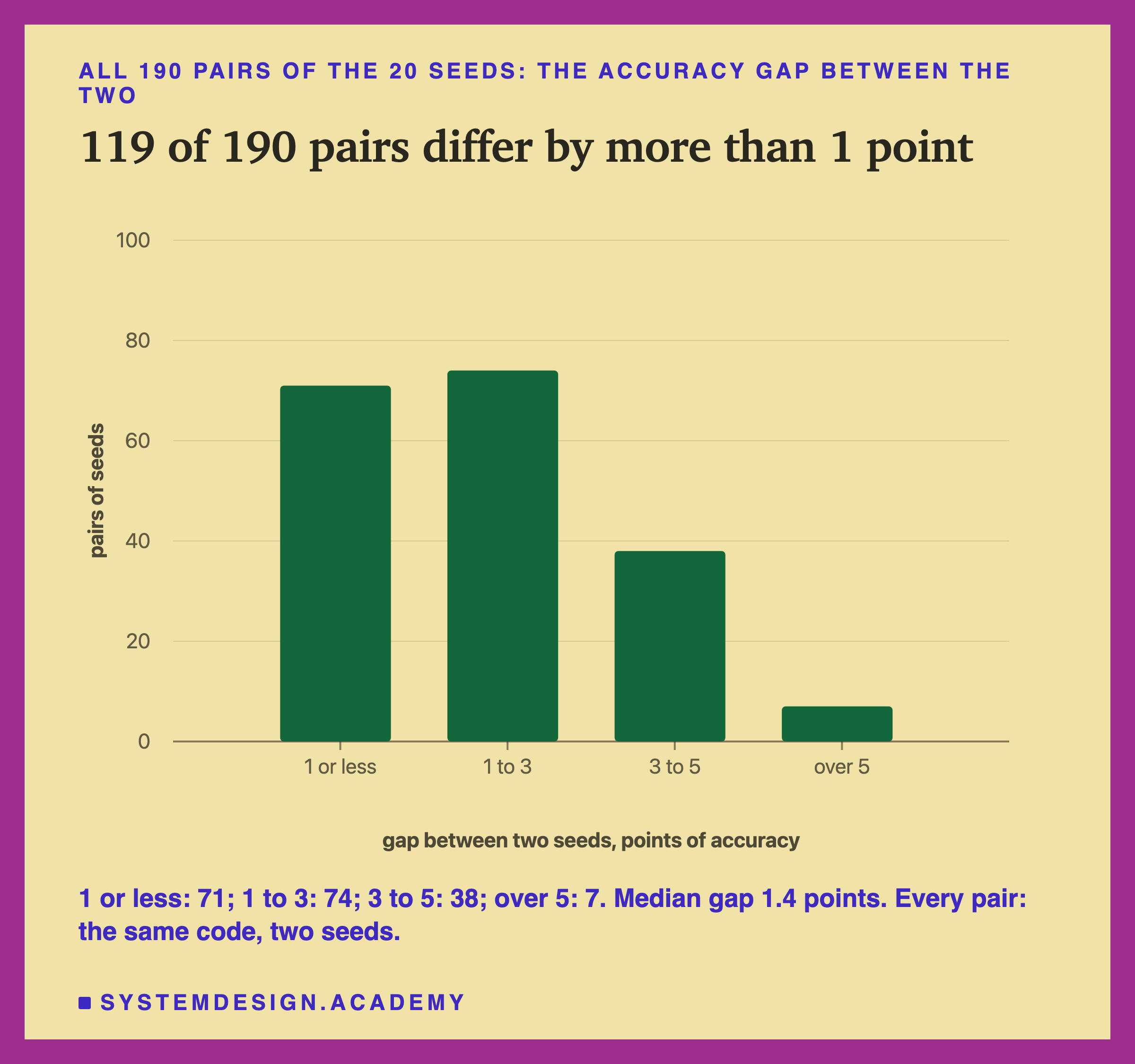
There are 190 ways to pick two of the 20 seeds, and every pair is the same code on the same data. The median gap between the two scores was 1.4 points, and 7 pairs were more than 5 points apart. Now suppose a team sees a 2-point gain after a change, measured with one run on each side. Here, 70 of the 190 pairs of seeds were more than 2 points apart with nothing changed at all. A 2-point gain from one run each is well inside what the seed alone produced.

Here is the same problem as a real decision: should early stopping be on or off for this model?

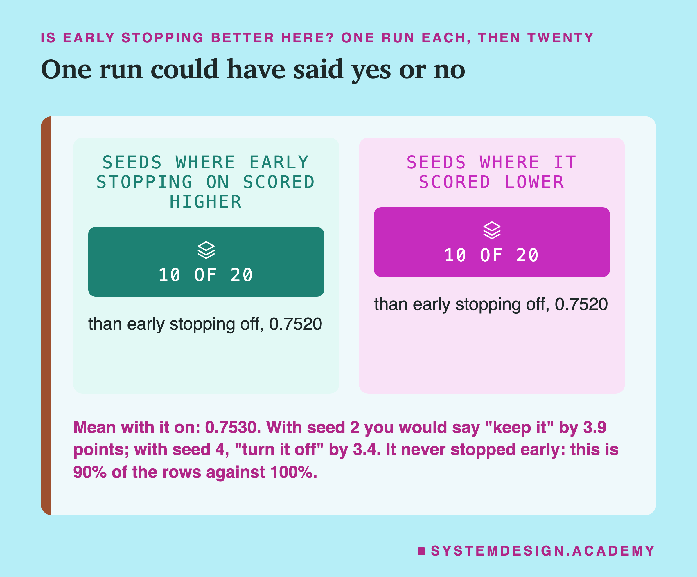
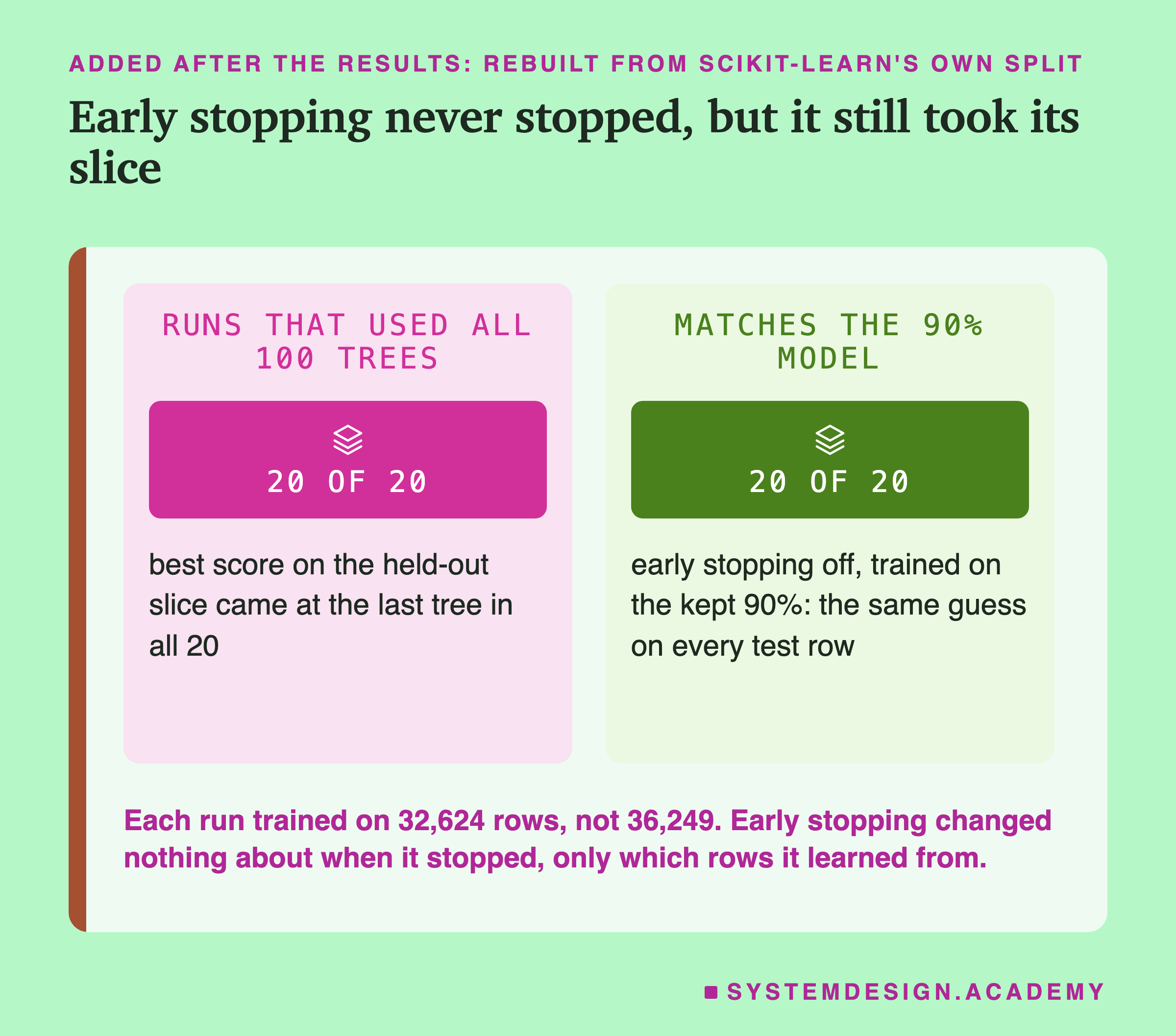
With early stopping off, every seed gives 0.7520. With it on, the seed decides. If you had run seed 2, early stopping would look 3.9 points better and you would keep it. If you had run seed 4, it would look 3.4 points worse and you would turn it off. Over all 20 seeds it came out higher 10 times and lower 10 times, with a mean of 0.7530 against 0.7520. Be clear about what this compares: early stopping never stopped here, so the comparison is really training on 90% of the rows against training on 100%, not the benefit of stopping early. On this data that choice made no clear difference on average and made the result depend on luck. One run each could have told you either story with confidence.

The pipelines lesson named three inputs to freeze: data, code and environment. This lab adds detail to each, and a fourth, the seed.

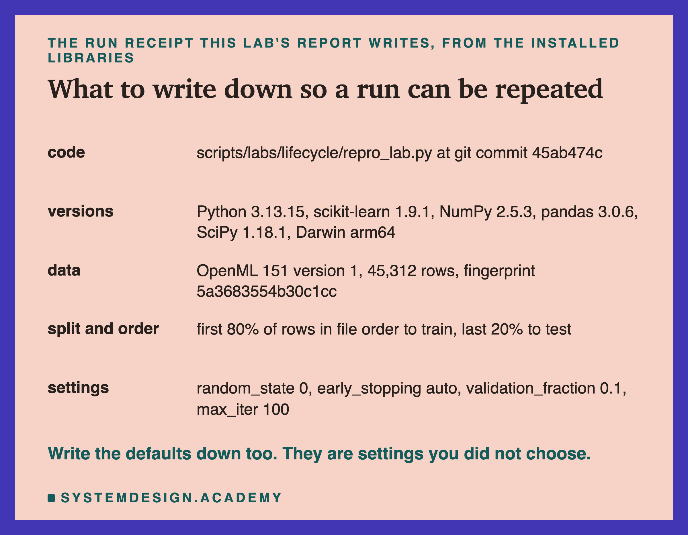
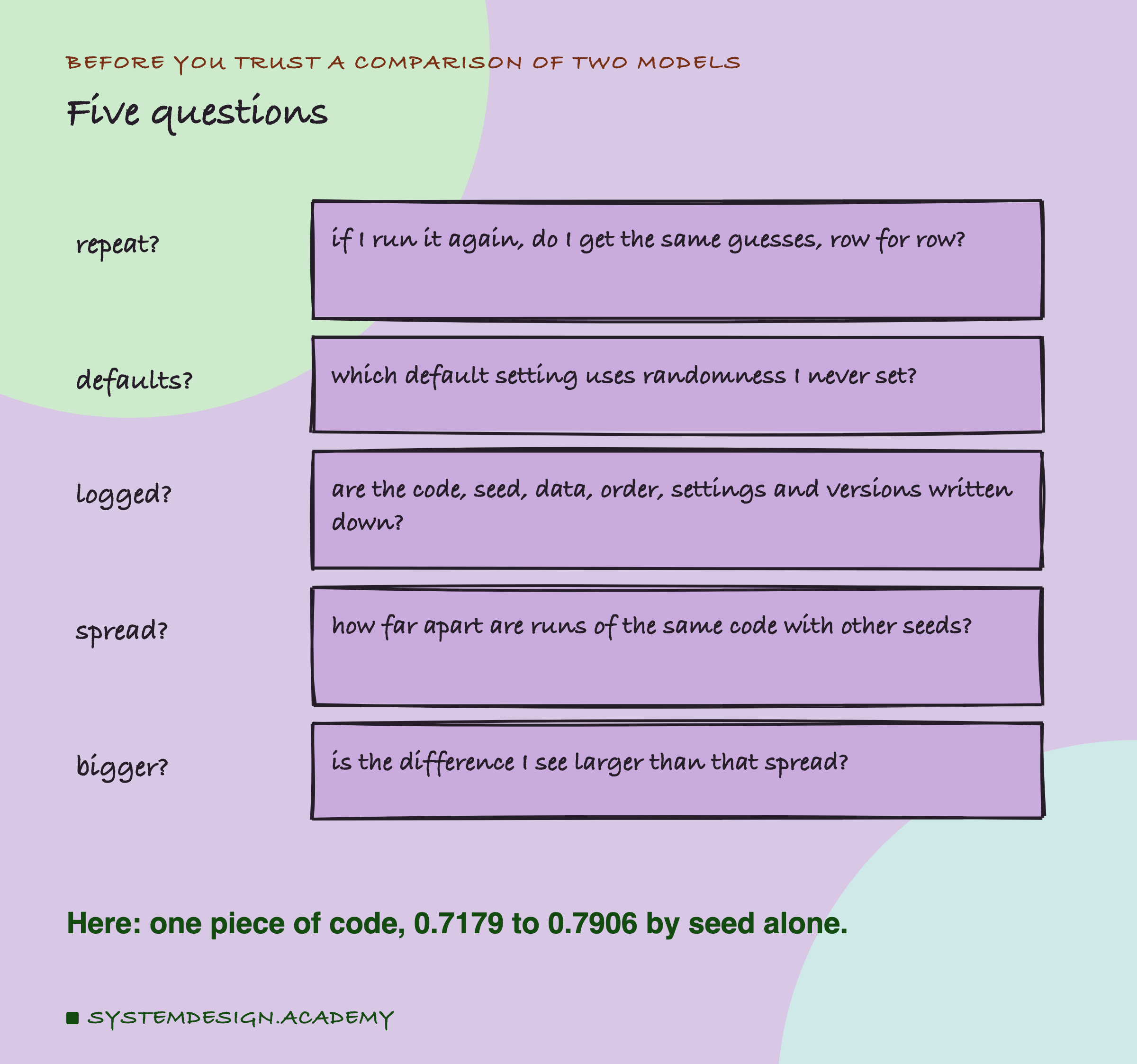
The code. Commit the training code before the run and record the commit. A git commit is a saved version of the code with a short name, such as 45ab474c for the commit that last changed repro_lab.py. Without it, nobody can tell whether two runs used the same code.

The seed. Set random_state on every model and every split, and write it down. Here, with the code, data, order and versions unchanged, seed 0 gave one model in 20 runs.

The data snapshot and its order. Save the exact rows, and a fingerprint: a short code computed from the bytes of the data (here a SHA-256 hash), which changes if a single value changes. Keep the order of the rows, or sort by a fixed key before training. Here the order changed the model through the slice.

Every setting, defaults included. The setting that moved this model was one I never wrote. Log the full list of settings the model actually used; in scikit-learn, model.get_params() returns them all.

The library versions. A default can change between versions of a library, and so can the way a split draws its rows. Write down the version of Python and of every library. The report does it with sklearn.__version__ and the like.

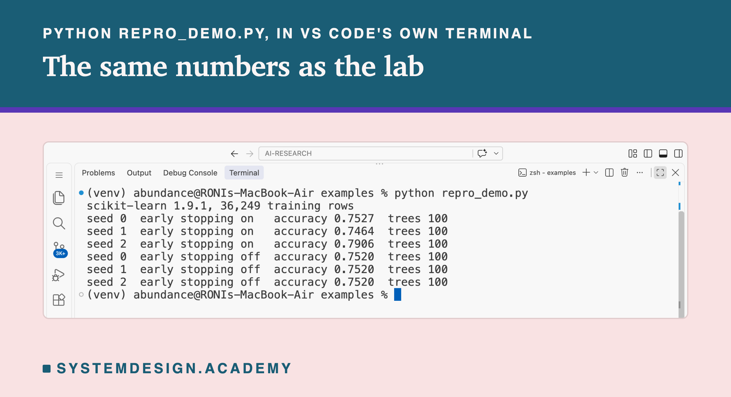
This script is the lab made small. It downloads the same data, trains the boosted trees with seeds 0, 1 and 2, first with the default settings and then with early stopping off, and prints each accuracy and the number of trees built. It does not need a GPU.

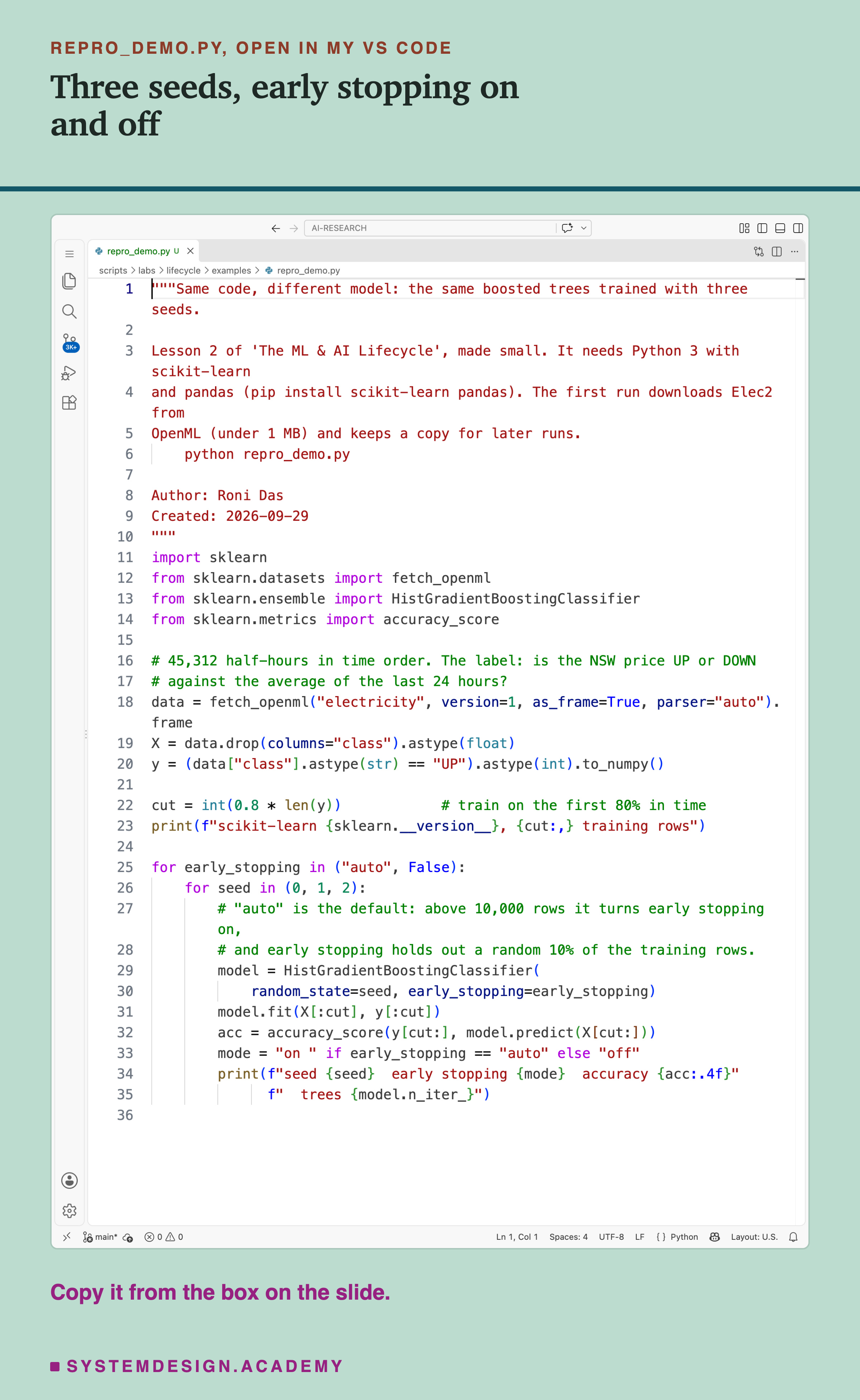
Before you run this lab. You need Python 3 and two libraries: pip install scikit-learn pandas. scikit-learn holds the model, the score and the download; pandas holds the table. The first run downloads Elec2 from OpenML (under 1 MB compressed), so it needs an internet connection once; scikit-learn keeps a copy in a folder in your home directory (scikit_learn_data) for later runs. I ran it with scikit-learn 1.9.1 on a Mac. scikit-learn runs the same way on Windows and Linux, but I have not checked the numbers there. This lesson is about exactly that: another version of scikit-learn, or another machine, may give different decimals, and the first line the script prints is the version, so you can compare.

"""Same code, different model: the same boosted trees trained with three seeds.

Lesson 2 of 'The ML & AI Lifecycle', made small. It needs Python 3 with scikit-learn
and pandas (pip install scikit-learn pandas). The first run downloads Elec2 from
OpenML (under 1 MB) and keeps a copy for later runs.
    python repro_demo.py

Author: Roni Das
Created: 2026-09-29
"""
import sklearn
from sklearn.datasets import fetch_openml
from sklearn.ensemble import HistGradientBoostingClassifier
from sklearn.metrics import accuracy_score

# 45,312 half-hours in time order. The label: is the NSW price UP or DOWN
# against the average of the last 24 hours?
data = fetch_openml("electricity", version=1, as_frame=True, parser="auto").frame
X = data.drop(columns="class").astype(float)
y = (data["class"].astype(str) == "UP").astype(int).to_numpy()

cut = int(0.8 * len(y))            # train on the first 80% in time
print(f"scikit-learn {sklearn.__version__}, {cut:,} training rows")

for early_stopping in ("auto", False):
    for seed in (0, 1, 2):
        # "auto" is the default: above 10,000 rows it turns early stopping on,
        # and early stopping holds out a random 10% of the training rows.
        model = HistGradientBoostingClassifier(
            random_state=seed, early_stopping=early_stopping)
        model.fit(X[:cut], y[:cut])
        acc = accuracy_score(y[cut:], model.predict(X[cut:]))
        mode = "on " if early_stopping == "auto" else "off"
        print(f"seed {seed}  early stopping {mode}  accuracy {acc:.4f}"
              f"  trees {model.n_iter_}")

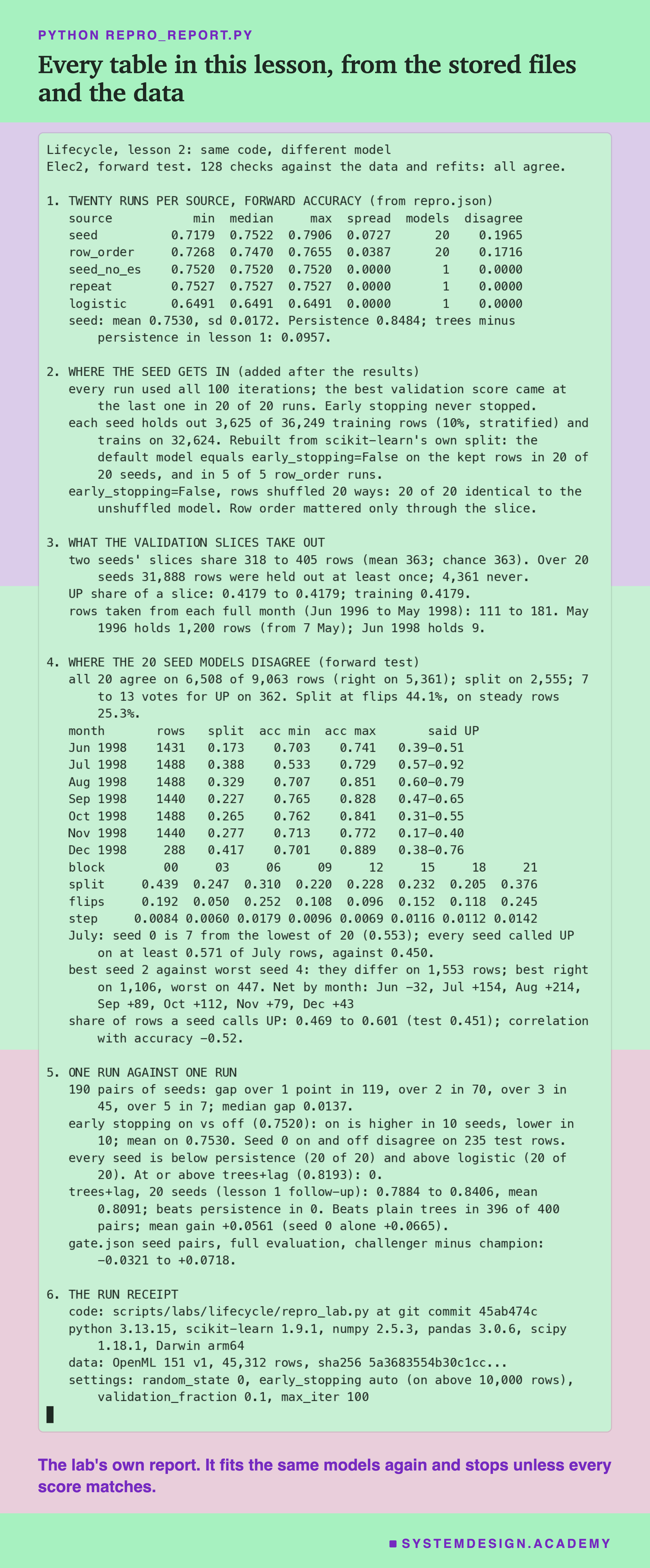
The report lives in scripts/labs/lifecycle/repro_report.py. It reads the lab's stored file, results/repro.json, lesson 1's results/baseline.json and results/baseline_followup.json, the gate lab's results/gate.json, and the Elec2 data from scikit-learn's local copy. The lab stored accuracies, not guesses, so the report trains the lab's models again and compares each accuracy with the stored one to twelve decimal places: seeds 0 to 19 with the default settings, where it also checks that each built 100 trees; seeds 0 to 19 with early stopping off; the 20 shuffles; the repeat, trained twice, which must give the same guesses both times; and logistic regression with seeds 0 and 7, which must give the same guesses. It changes nothing in repro.json.

It also runs the checks I added after the results: it rebuilds each seed's validation slice from scikit-learn's own split and trains a no-early-stopping model on the rest (20 of 20 identical), trains the 20 shuffles with early stopping off (20 of 20 identical to the unshuffled model), rebuilds the slice for 5 of the 20 shuffles (5 of 5 identical), and checks that the 10 gate-lab pairs within seeds 0 to 19 use this lab's seeds. Then it prints the tables in this lesson and the run receipt. It makes 128 checks in all, and they all agree.

Its mode writes every number to , which the figures read. The mode checks the student script's stored run, and the mode writes the playground below and checks that it gives the lab's 20 accuracies.

This box has no model in it. It holds the 9,063 forward test labels and the guesses of all 20 seed models for every row, recomputed by the report and checked against the lab's 20 accuracies. Each guess is a 0 or a 1, so the 20 guesses for one row can be written as a single 20-digit binary number, one digit (a bit) per seed. To keep the box small, that number is written in hexadecimal, counting in sixteens with the digits 0 to 9 and a to f, which takes five characters instead of twenty. The guesses function unpacks it for you. It runs in your browser.

As it is, the box prints each seed's accuracy, from 0.7179 to 0.7906 with a spread of 0.0727, which the report's box mode checks against repro.json, and then compares seed 2 with seed 4: they differ on 1,553 rows, and seed 2 is right on 1,106 of them.

Try by_month(2, 4) to see the best and worst seed month by month, and votes() to see how many of the 20 models said UP on each row. Try compare(0, 1) for two neighbouring seeds. Then pick two seeds and pretend they were two versions of a model, a "before" and an "after". How big a gain would you have believed?

Loading. fetch_openml("electricity", version=1) downloads Elec2 once and reads the local copy after that. The label column holds the words UP and DOWN, turned into 1 and 0. The eight inputs become plain numbers with astype(float), as in the lab.

The version line. sklearn.__version__ is printed first, because the result depends on it. If yours is not 1.9.1, the accuracies may differ.

The cut. cut = int(0.8 * len(y)) is 36,249. The model learns from X[:cut] and is scored on everything after. Nothing is shuffled.

The two loops. The outer loop sets early_stopping to "auto", the default, and then to False. The inner loop sets random_state to 0, 1 and 2. Each pass builds a fresh model, so nothing carries over between runs.

What "auto" does. With more than 10,000 training rows, "auto" turns early stopping on, and early stopping holds out a random 10% of the training rows, chosen by random_state. With False, all 36,249 rows are used and has nothing to choose here.

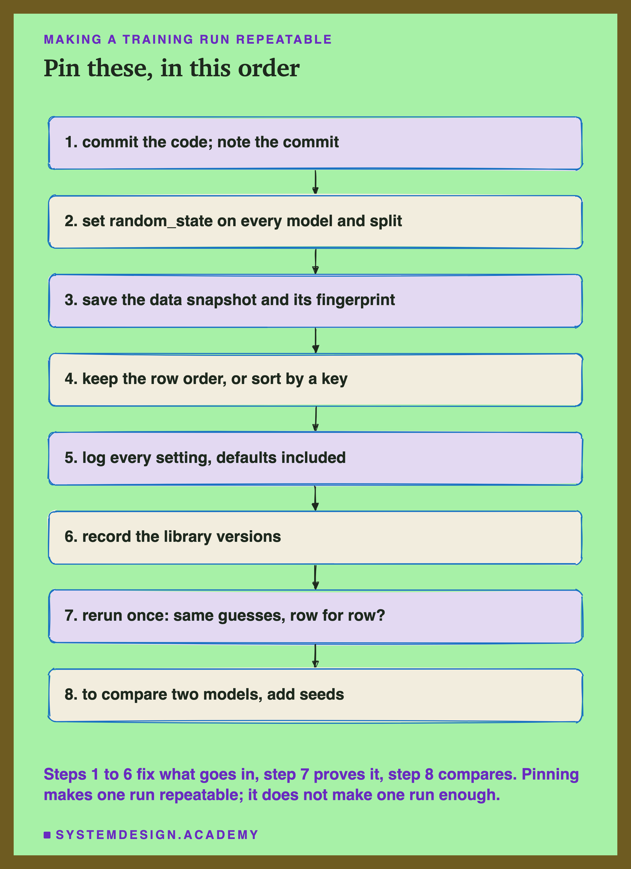
The order matters: first fix everything that goes into the run, then prove the run repeats, and only then use it to compare models.

Commit the code. Train from a committed version of the code, never from unsaved changes, and record the commit.

Set random_state everywhere. On every model and every split, including splits you did not write, such as the one inside early stopping. If a library has a global random generator, set that too.

Save the data, not a query. A query against a live table can return different rows tomorrow. Save the exact rows, or a versioned snapshot, with a fingerprint.

Keep the order. Sort by a fixed key, such as time and then an id, before training. A database or a file system does not promise the same order twice.

Log every setting. Log get_params(), not just the settings you typed. Read the documentation of every default that uses a seed, a sample or a split.

Record the versions. Python, every library, and the machine type. A lockfile, a file listing the exact version of every library, does this for a whole project.

Rerun once, and compare guesses. Train again from the receipt and check that every guess matches. A matching score is not enough.

Then, to compare two models, add seeds. Run the change with several seeds, for example five or ten, and look at the spread before you believe a gain.

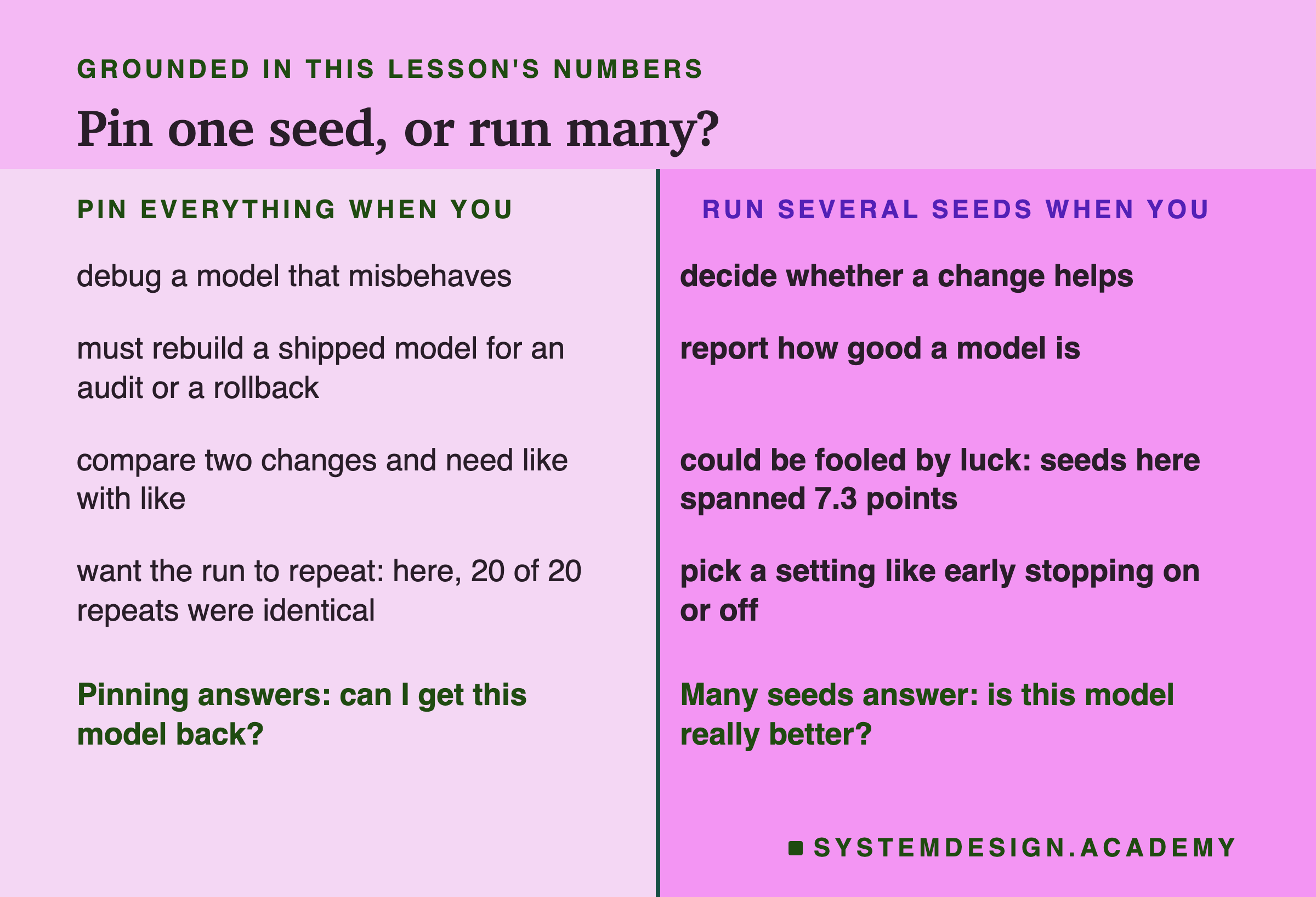
Pin everything when you need a model back. Debugging, audits and rollbacks all need the exact model, and a pinned run gives it: here 20 runs of seed 0 gave one model every time.

Pin everything when you compare two changes on one seed. Same seed, same rows, same order, same versions, so that the change you made is the only difference. That is a fair comparison of two models, for that seed.

Run several seeds when you decide whether a change helps. One pinned seed can still be a lucky or an unlucky one: here seed 2 would have made early stopping look good and seed 4 bad. Report the spread, not one number.

Run several seeds before you report a score to anyone. The score of one seed is one draw. The median and the range of several is the honest summary. Here that is a median of 0.7522 and a range of 0.7179 to 0.7906.

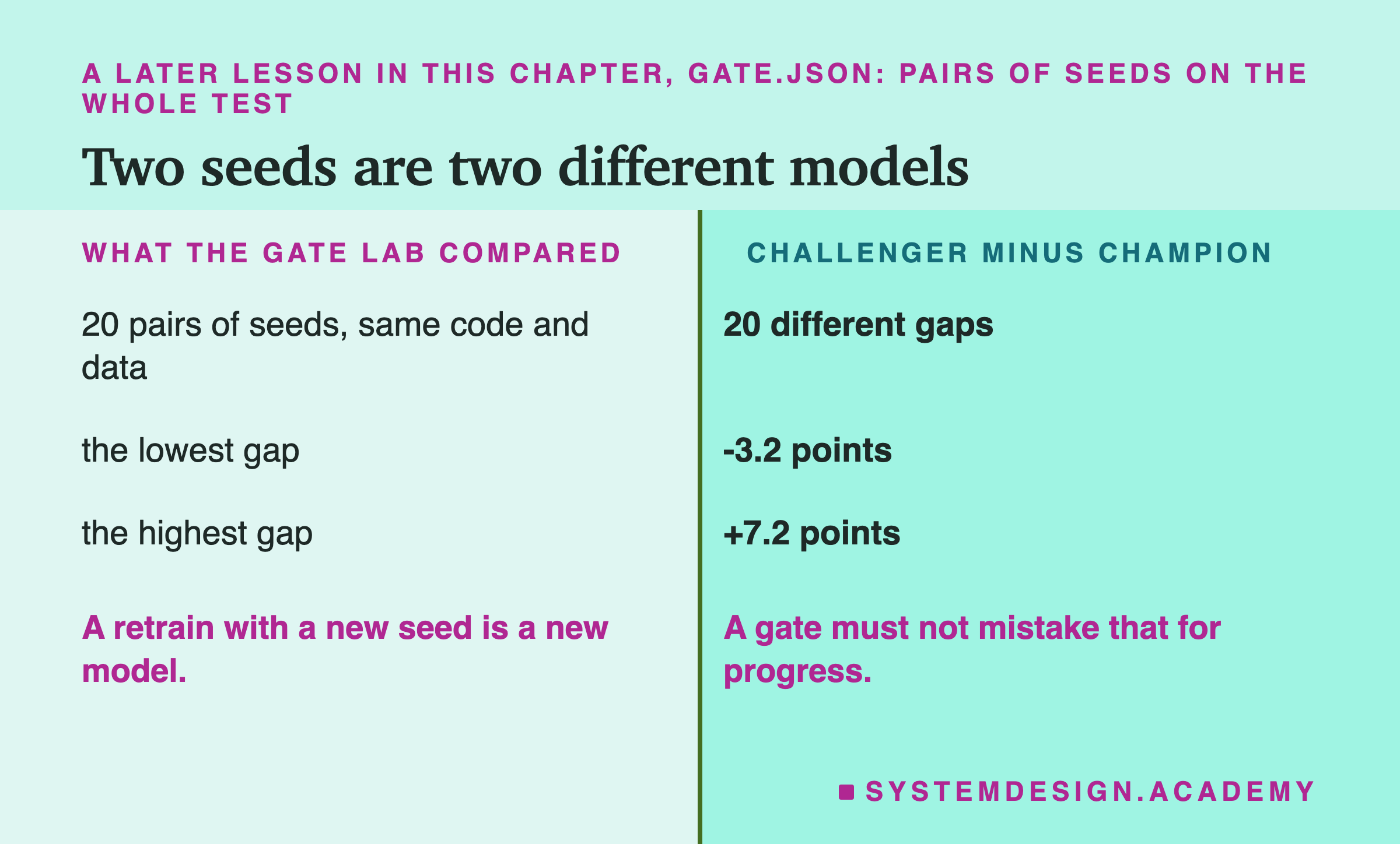
Do not pin a seed and then pick the best one. Trying many seeds and shipping the highest scorer on the test turns the seed into a setting you tuned on the test. A later lesson in this chapter measures how much of such a winner's lead is luck.

Do not expect pinning to survive a change of version or machine. A new library version can change a default or the way a split draws rows. Pinning holds within one recorded environment.

Removing the randomness is not always the answer. Here, turning early stopping off removed the spread and scored about the same as the average. With other data, early stopping can really help. Measure it over several seeds before you decide.

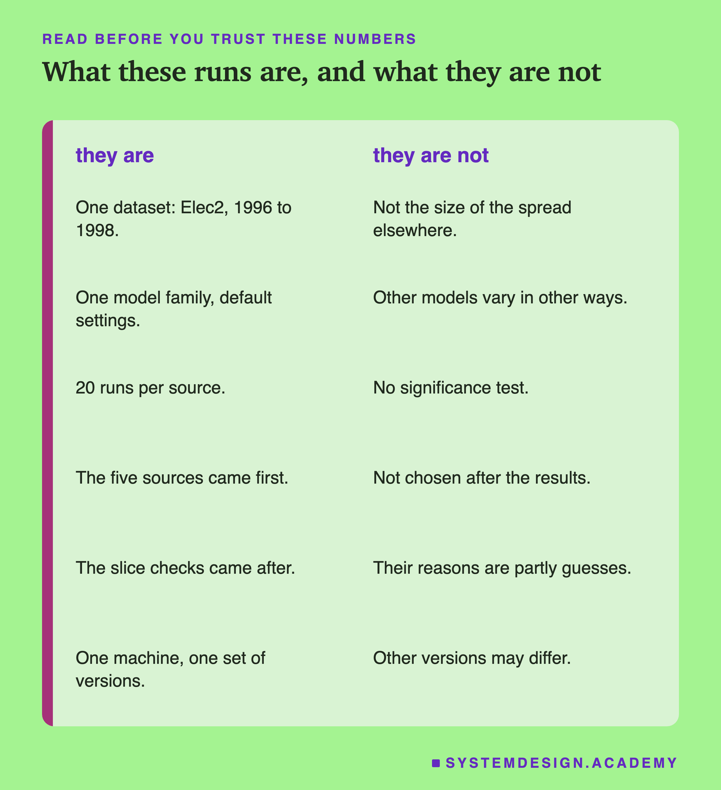
One dataset, one model, default settings. The size of the spread, 7.3 points, belongs to these trees on this data and this split. With more training rows, or a test more like the training period, the slice would probably matter less; I did not test that. Neural networks and other methods have other sources of randomness, such as the starting weights and the order of batches, which this lab does not cover.

20 runs per source, no significance test. The design described the runs and declared no test. The correlation of -0.52 between calling UP and accuracy is over 20 points and is a pattern, not a proof.

The design came first; the explanations came after. The five sources and the stored measures were written in repro_lab.py before it ran. Reading the scikit-learn source, rebuilding the slices, the shuffled runs with early stopping off, and every table of where the seeds disagree were added after I saw the results. The slice was rebuilt for all 20 seeds but for only 5 of the 20 shuffles.

What is measured and what is guessed. Measured: the default model makes the same guesses as a no-early-stopping model trained on the rows the slice left, for all 20 seeds; row order mattered only through the slice, for these trees. Guessed: why July split most. Not explained: why night rows split most; the two reasons I checked did not fit.

One machine, one set of versions. Everything ran on one Mac with scikit-learn 1.9.1. I have not checked whether another version or another operating system gives the same models. The lesson's advice is to record that, because I cannot promise it.

The dates are rebuilt, as in lesson 1: months and hours come from row numbers, checked against the weekday column.

Take the last model your team trained and try to rebuild it from what was written down. If you cannot, find what is missing: usually the code version, the data snapshot, the seed of some split, or the library version. Then train it five times with five seeds and write down the spread. Put that number next to the last improvement anyone claimed for the model. If the improvement is smaller than the spread, measure it again with several seeds before you believe it.

It takes an afternoon. The receipt it produces is the start of everything later in this chapter: a pipeline can only promote, roll back and compare models whose runs it can repeat.

The next lesson planned for this chapter takes the other road out of this lesson: if a team tries many settings or many seeds and keeps the best, how much of the winner's lead is luck, and how much of it survives on fresh data?