The Library That Sent Its Books Back
Imagine a small library that has run out of shelf space. The librarian has a plan. Every new book that arrives, she reads, writes a one-page summary for the card index, and sends the book back to the publisher. The index stays small and tidy. Anyone who asks "what is this book about?" gets a good answer in seconds.
Then, one day, a reader asks something new. "What does chapter seven say about the town's old railway?" The summary does not say. It was written for the questions people asked back then, and nobody asked about railways. The book is gone, so the question has no answer.
A second library keeps every book on the shelf and writes a summary only when a reader asks for one. Its shelves cost more. But when the railway question comes, the book is still there.
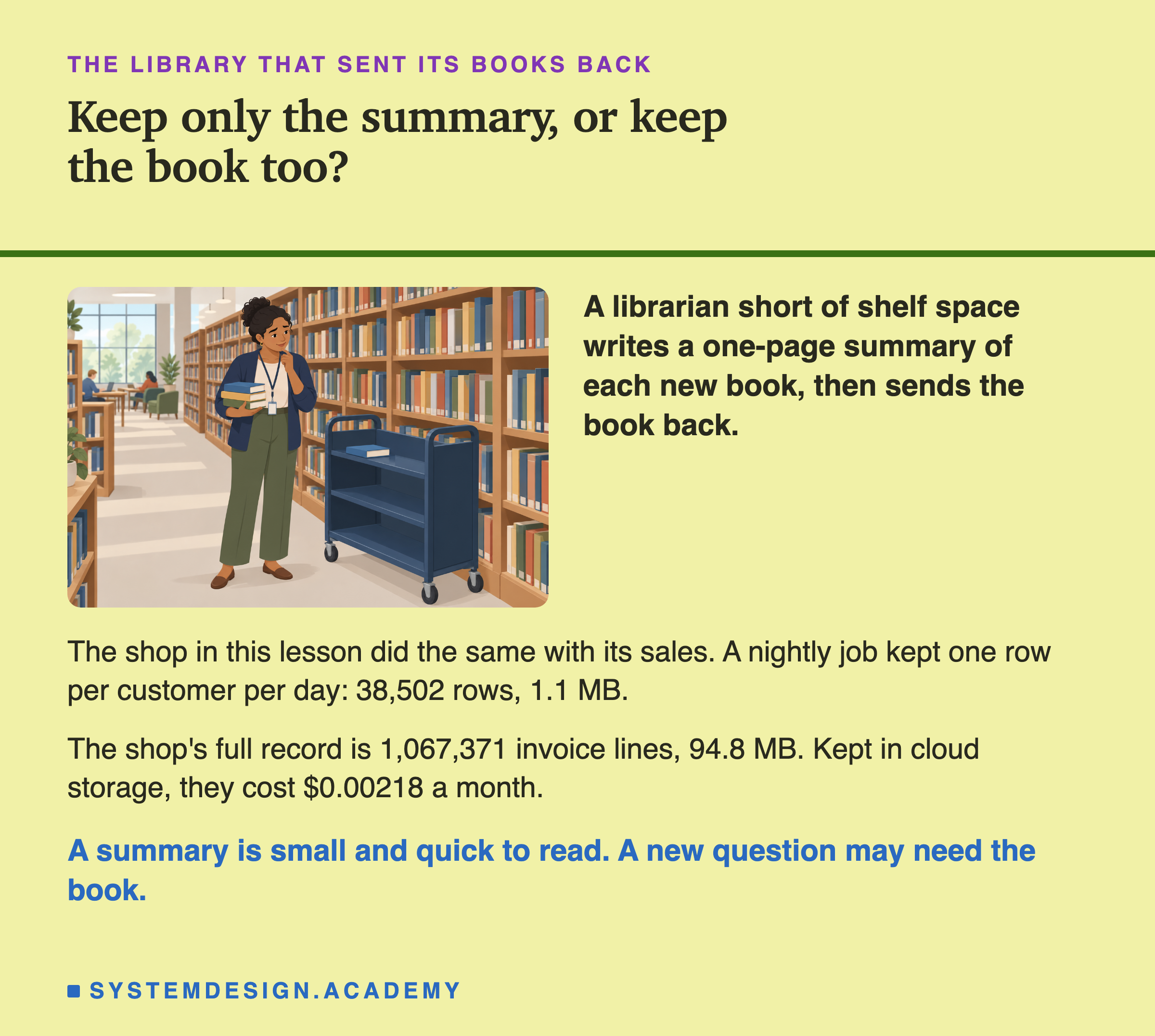
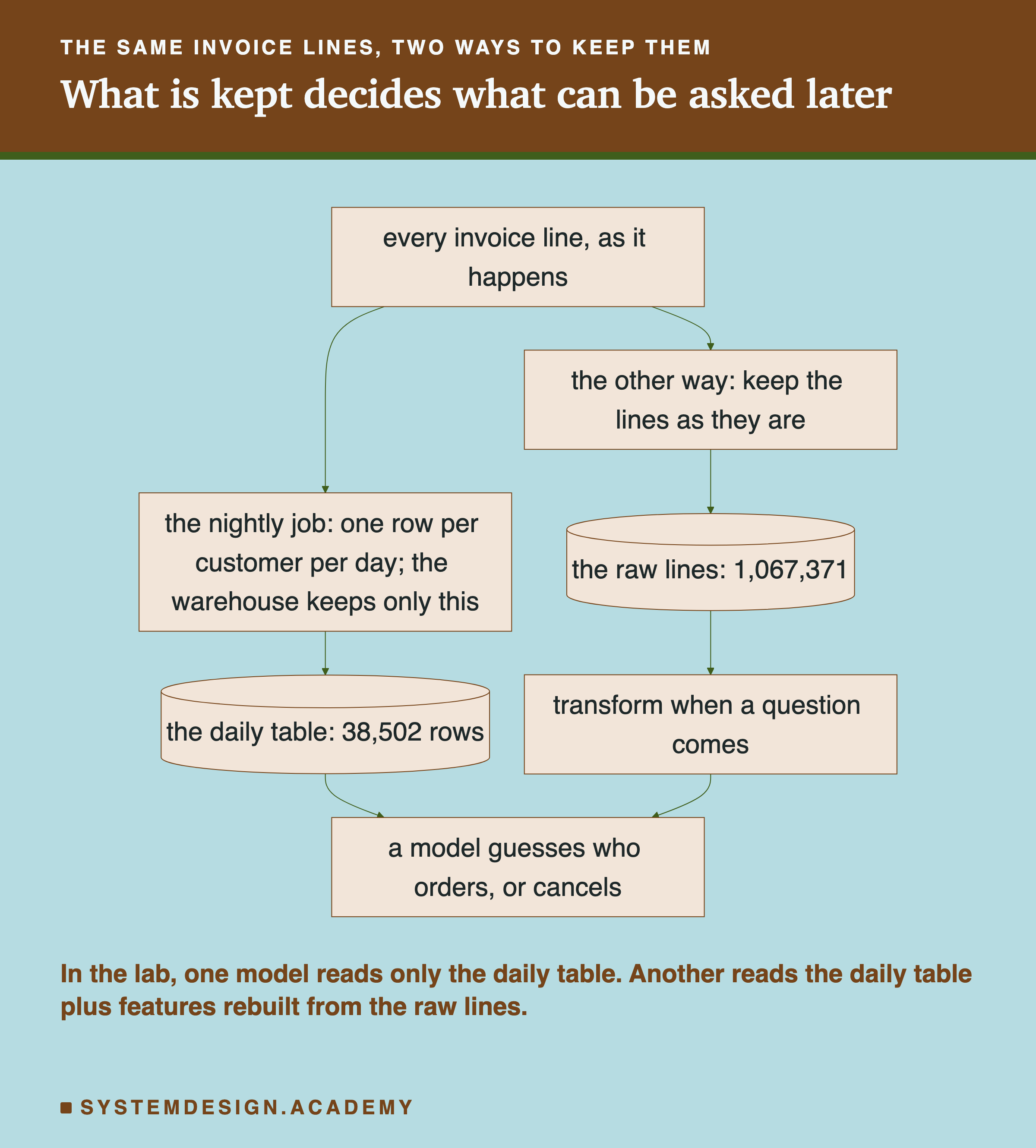
Many companies make this same choice with their data every night. A shop takes each day's sales and adds them up into a neat summary, one row for each customer for each day. That summary is what the finance team wants. The question is what happens to the sales lines that were added up.
In this lesson I measure that choice on a real online shop. Its summary has 38,502 rows, built from sales lines that the warehouse did not keep. The shop's full record is 1,067,371 lines. Keeping those lines in cloud storage would have cost $0.00218 a month. The rest of the lesson asks what the lines were worth when new questions came.
Where This Lesson Starts
This is the third lesson of the chapter on data engineering for machine learning. The first lesson asked how fresh each number needs to be. The second, data ingestion pipelines, covered how data gets copied out of the systems where it is made. This lesson asks what happens next: in what order the data is cleaned and stored, and what that order keeps.
Here is the plan. First I name the parts. Then I show the two orders side by side, where each one does its work, and what each one costs. Then comes a small lab on real data, from a real shop. After that, the ideas teams use to keep their stored data in order, and the cases where the old order is still right.
The shop's data is public, so you can run every step yourself. The lab has one script, which builds the nightly summary and trains eight models: four designs, for each of two questions. A second script checks every number the first one printed, by a different method. Where I could measure something, I did. Where I could not, such as what a real cloud bill would be, I say so.
Ten Words for This Lesson
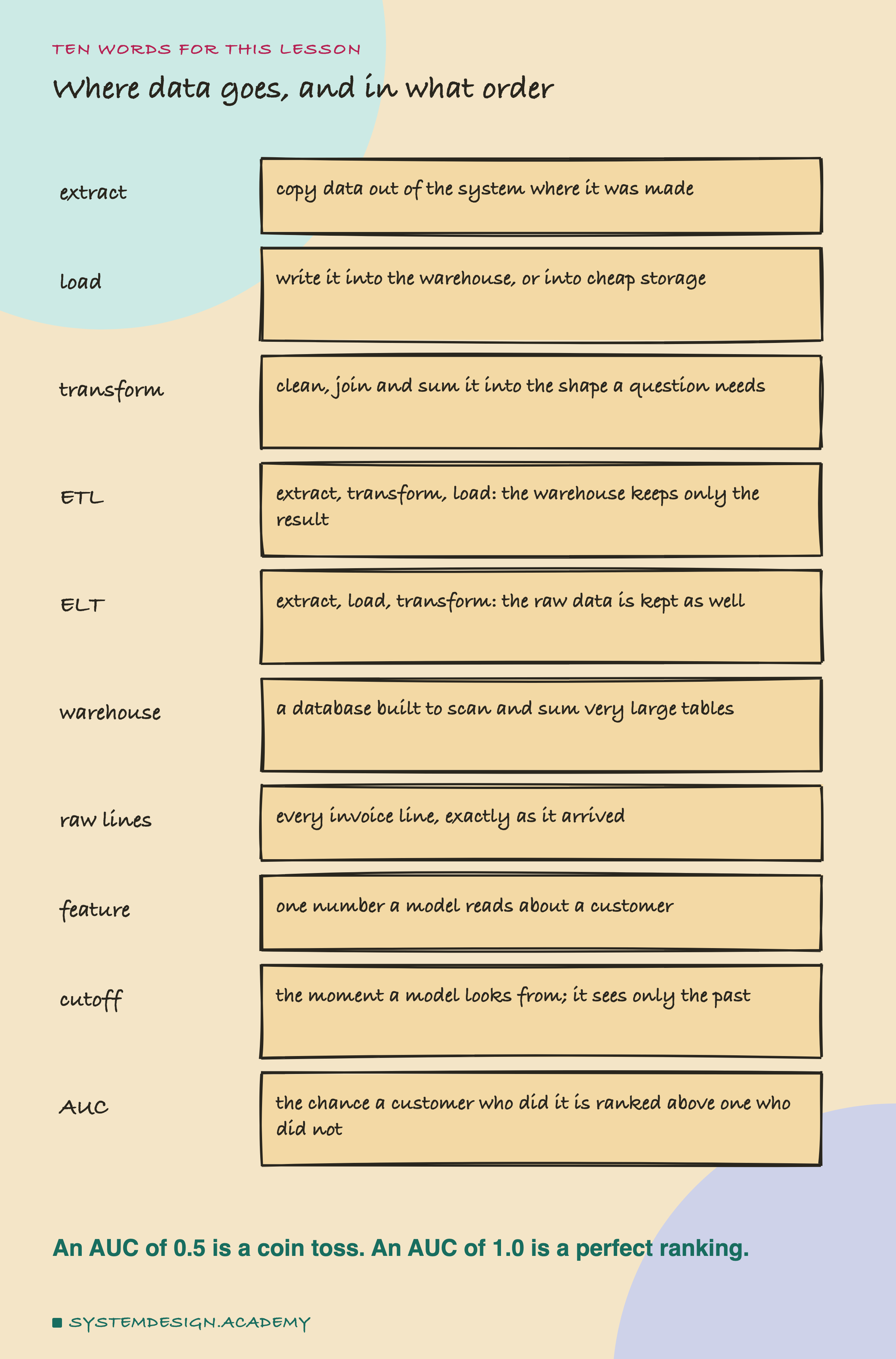
Three steps move data from where it is made to where it is used. To extract is to copy the data out of the system that made it, such as a shop's app database. To load is to write it into the place where it will be kept and read. To transform is to clean it, join tables together and add rows up into the shape a question needs.
ETL means extract, transform, load, in that order: the data is cleaned and summed first, and the warehouse stores only the result. The raw rows live on only if the source database, or an archive, still keeps them, and a source database may delete old rows after a while. ELT means extract, load, transform: the raw data is stored first, as it arrived, and the transforms run later. A warehouse is a database built to scan and add up very large tables, such as Snowflake or Google's BigQuery.
A feature is one number a model reads about a customer, such as the days since their last order. A model learns from features. The cutoff is the moment a model looks from. It may use only what happened before the cutoff, and it guesses what happens after.
To score the guesses I use AUC, short for area under the curve. Take one customer who did the thing and one who did not. AUC is the chance the model gives the first a higher score. An AUC of 0.5 is a coin toss, and 1.0 is a perfect ranking.
ETL and ELT: Same Letters, Different Order
ETL and ELT use the same three steps. Only the place of the T changes, and that one change decides what data survives.
In ETL, the transform runs before anything is stored, usually on its own machines: an older ETL tool, a Spark cluster or a Python job. Only the finished table is loaded. The warehouse never sees the raw data. It survives only if the source database or an archive keeps it.
In ELT, the raw data is loaded first, unchanged. The transforms run later, inside the warehouse, as , the language databases use for questions. The raw data stays, so any table can be rebuilt from it, or a new table built.
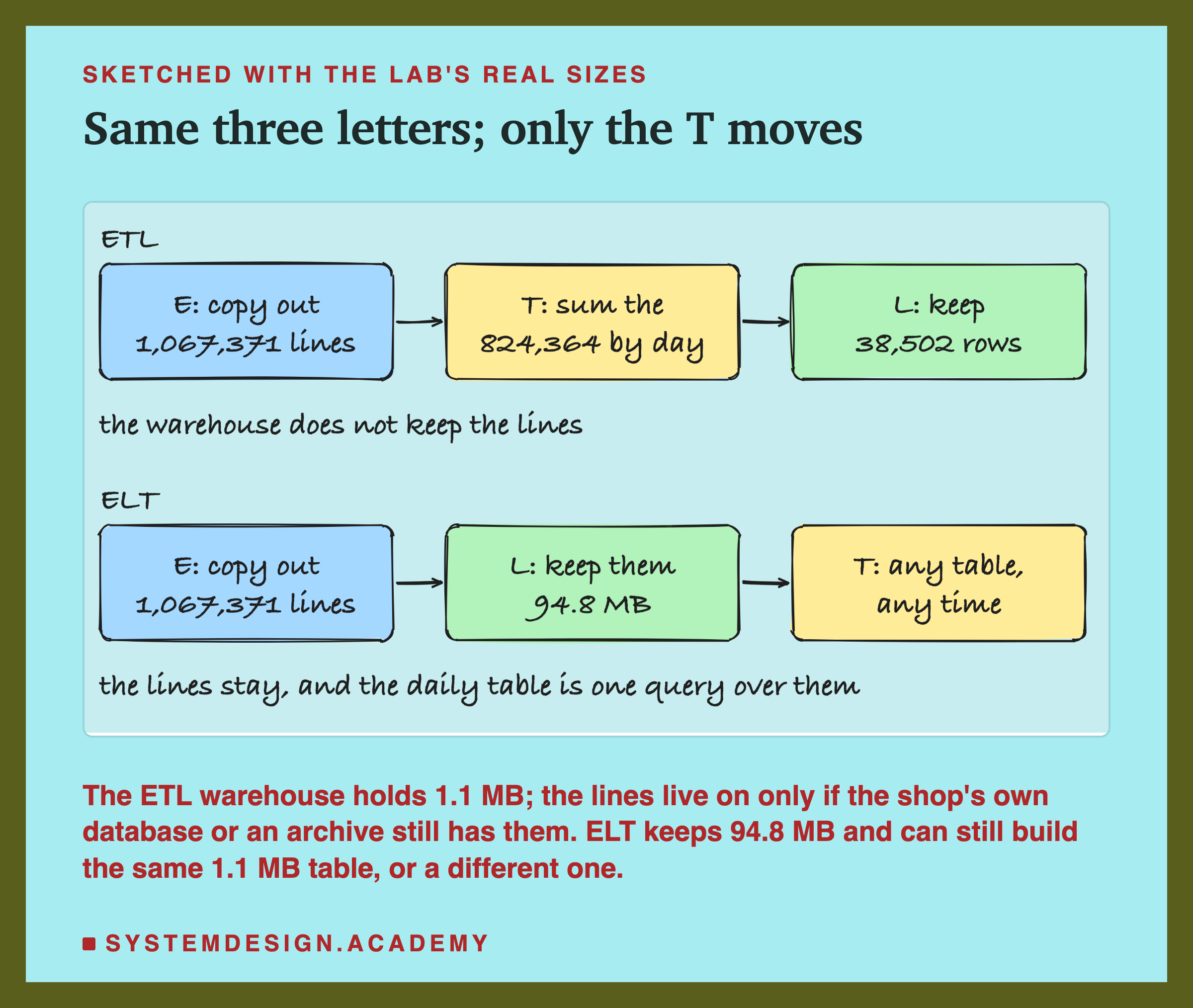
These are the lab's real sizes. The shop has 1,067,371 invoice lines. The nightly job read the 824,364 that have a customer id and kept 38,502 rows, one for each customer on each day they had a line. 5,390 of those days hold only cancellations. As text files, the lines take 94.8 MB and the daily table 1.1 MB. An ELT pipeline keeps the 94.8 MB and can build the same 1.1 MB table from it whenever it likes.
Notice what does not change. Both orders extract from the same sources. Both end up with clean tables for dashboards and models. Nobody argues that the transform can be skipped. The argument is only about order. Order decides three things: what you pay to store, where the compute runs, and which questions can still be asked next year.
ETL and ELT, Side by Side
The order swap spreads into cost, into who runs which machine, and into what a future model can ask for. It helps to put the two side by side, row by row, because neither one wins every row.
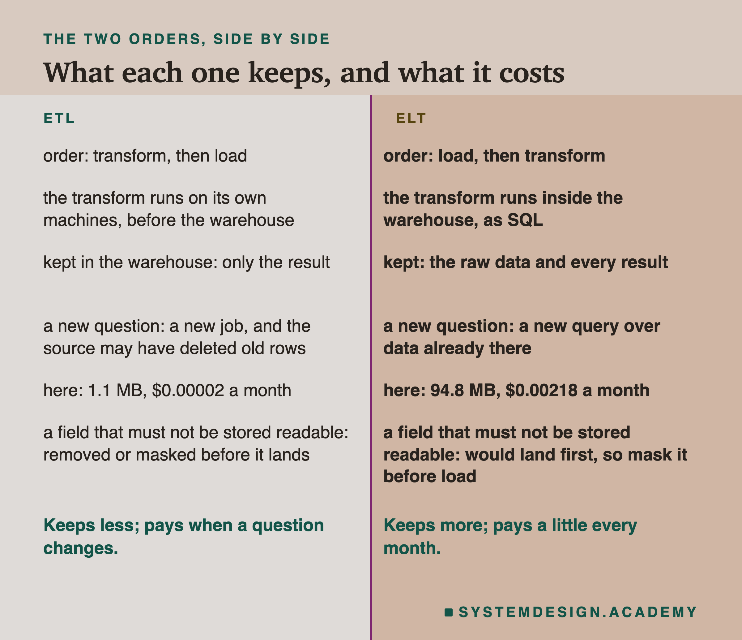
Read down a column to see one order as a whole. Read across a row to see the exact trade. Most rows favour ELT, and the storage row shows why the trade got easy: here, keeping everything cost two tenths of a cent a month more.
Look hard at the last row. It is the one place where ELT has no safe answer. Some fields must never be stored as they arrived. A card's security code must not be stored at all, and a card number may be stored only in a form nobody can read. For those fields the raw value must not land, so the transform has to come first. I come back to this near the end, because it is the clearest reason ETL is still used.
For machine learning, the row that matters most is the new question. With ETL, a feature the table never kept means a new job, and the history may already be gone. With ELT, the data is still there. The lab below measures how much that was worth, on real questions.
One Common Way to Build ELT
There are many ways to build an ELT pipeline. Here is one common shape, with real tools. The lab does all of it in a few lines of pandas, but the jobs are the same.
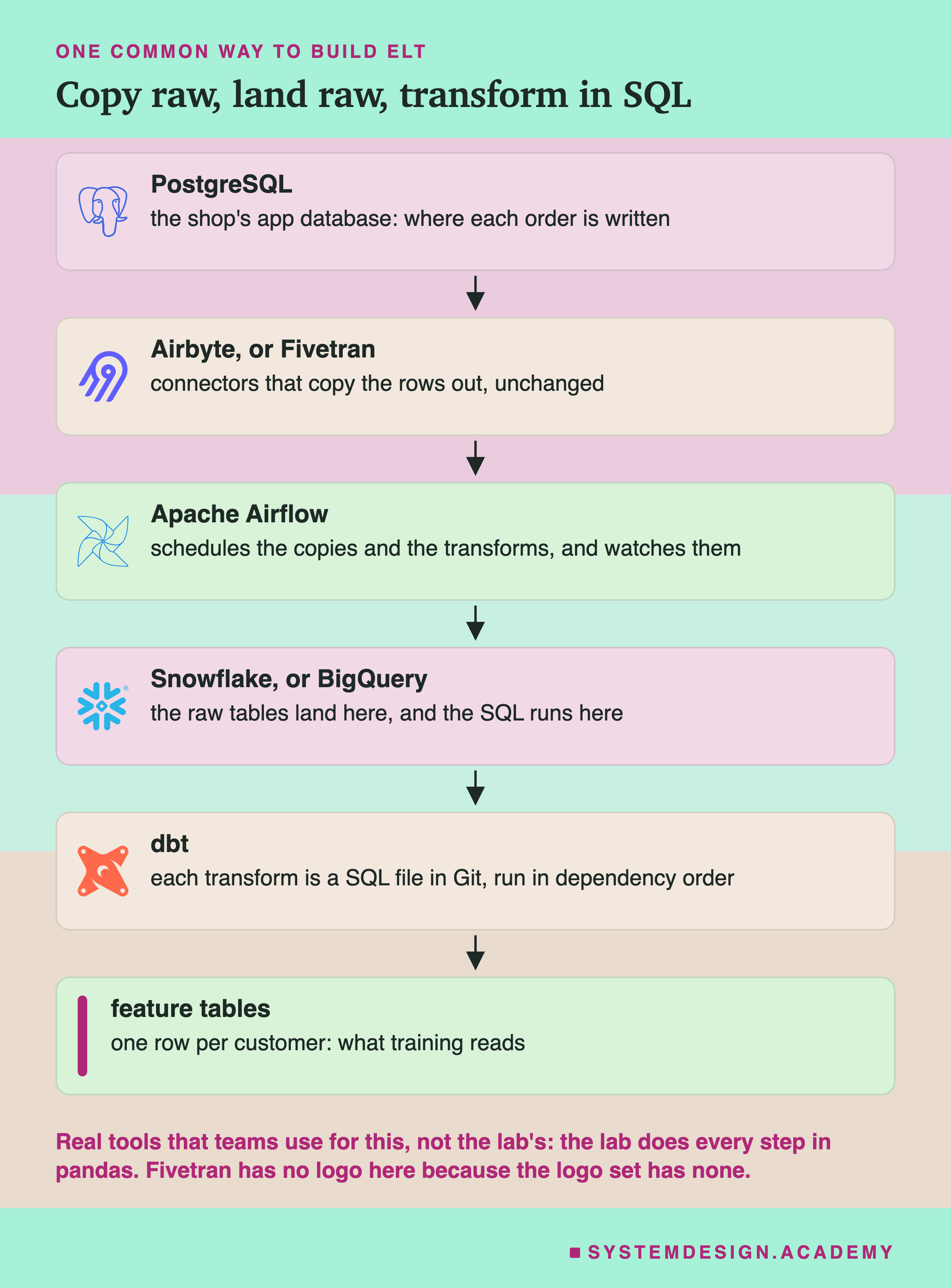
Each tool has one job. A connector such as Airbyte or Fivetran copies rows out of a source into the warehouse without changing them. Airbyte's connectors are open source; Fivetran is a commercial service. Airflow does not copy anything itself. It is a scheduler: in its own words, "a platform to programmatically author, schedule and monitor workflows".
dbt holds each transform as a file in Git, a system that keeps every version of a file, and runs the files in the right order. dbt calls each of these SQL files a model. That is a different thing from a machine learning model: a dbt model is one SQL query that builds one table. In this lesson, "dbt model" always means the SQL kind.
| Stage | What happens | Tools |
|---|---|---|
| Copy out | Rows are copied from each source, unchanged | Airbyte, Fivetran |
Where the Transform Runs
Here is the idea that makes ELT cheap to run: send the transform to the data, instead of pulling the data out to the transform.
In ETL, the data is pulled out to a separate cluster, a group of machines you run and pay for. Then the finished table is written into the warehouse. In ELT, dbt sends only the text to the warehouse. The warehouse runs it and writes the new table. No row comes back to dbt, and no second cluster runs.
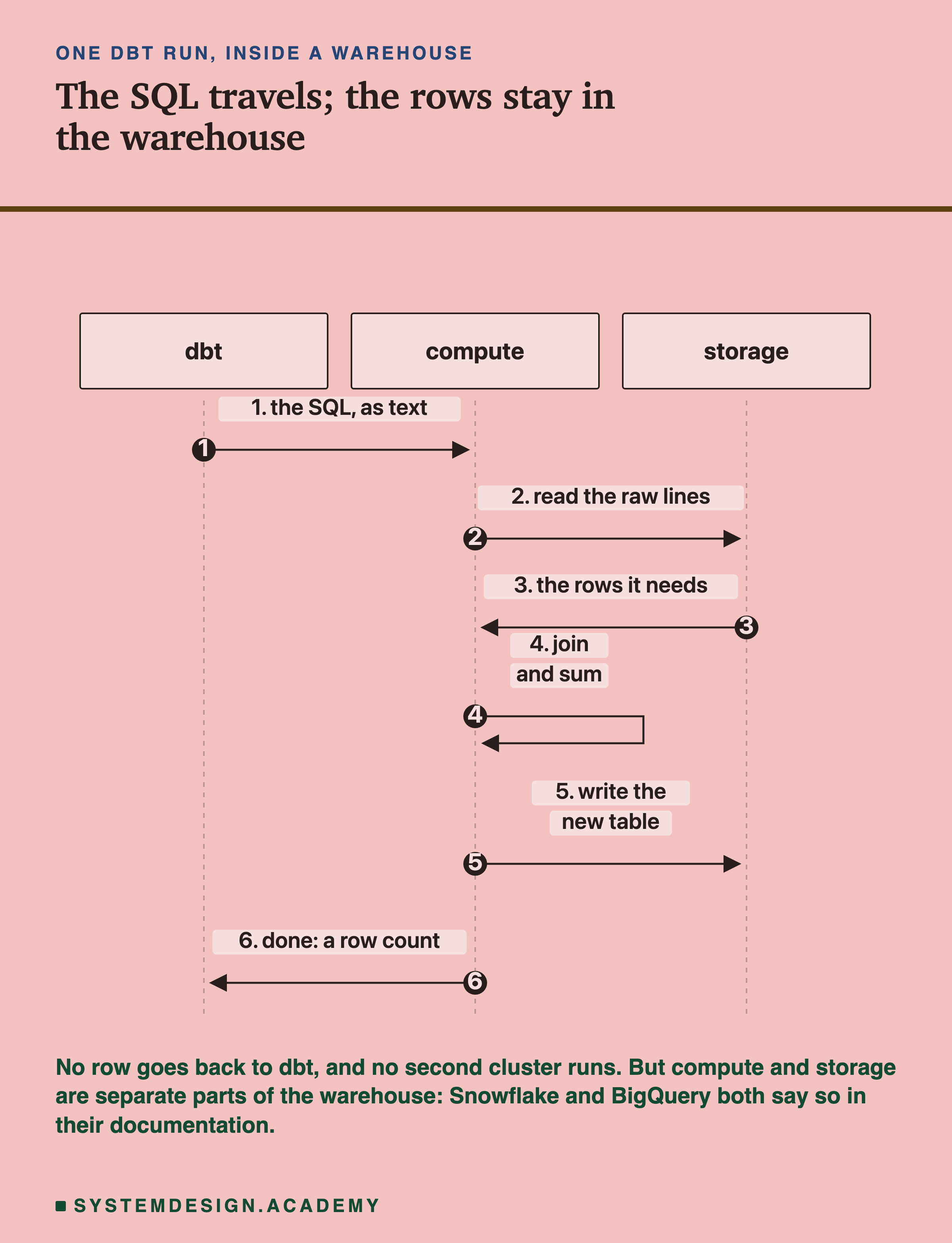
The old version of this lesson said the transform ran "on the same machines that store the data" and that "nothing moves across the network". For Snowflake and BigQuery that is wrong, and I have fixed it. Both keep storage and compute apart on purpose. Snowflake's documentation says it "separates storage and compute" and that "each virtual warehouse is an independent compute cluster". BigQuery's says "one of the key features of BigQuery's architecture is the separation of storage and compute".
So data does move, inside the warehouse, from its storage to its compute. What ELT removes is the trip out and back, and the second system to run. That split is also why compute can grow for one big job and then stop.
What Keeping the Raw Data Costs
The old version of this lesson had a chart of monthly cost against data size, with ETL rising to $11,500 a month and ELT to $2,900. No calculation or source stood behind either line, so I have taken it out. Here is what I could measure, with a real price.
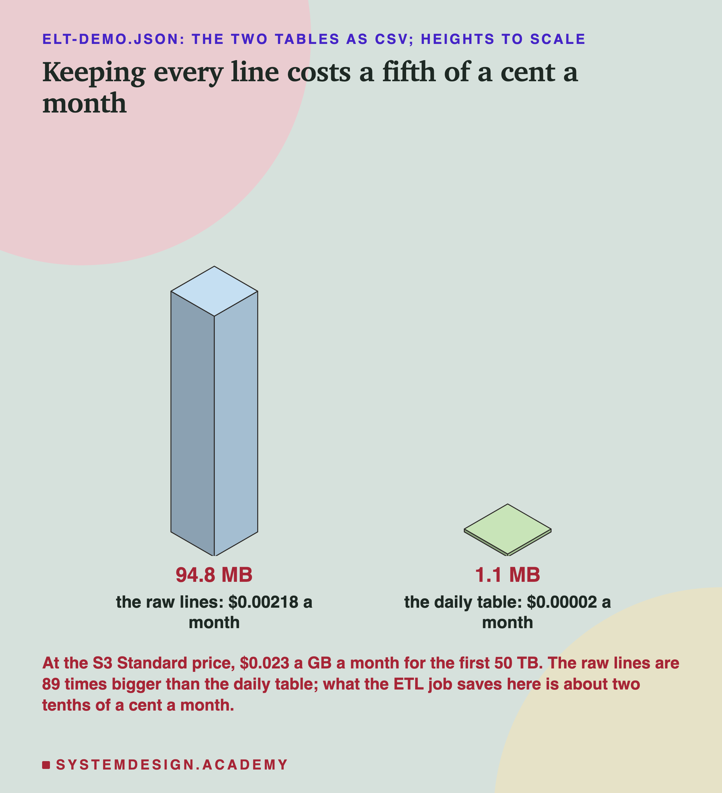
I wrote both tables out as CSV, plain text with commas between the values, and measured the bytes. The raw lines take 94.8 MB. The daily table takes 1.1 MB, 89 times less. Amazon S3, a cloud file store, lists $0.023 per GB a month for its Standard storage, the first 50 TB, in its US East region. At that price the raw lines cost $0.00218 a month and the daily table $0.00002.
This shop is small, so these are tiny numbers. The cost grows in step with size: a thousand times the data costs about a thousand times as much, around $2.18 a month. What matters is the shape. Storage is billed by the byte and by the month, and a byte costs very little.
Compute is billed differently. Snowflake bills a warehouse "per-second, with a 60-second (i.e. 1-minute) minimum", and can switch it off when idle. BigQuery's on-demand queries cost $6.25 per TiB of data read in its default US region, with the first TiB each month free. Either way you pay while a transform runs, not while it waits. I did not run any of this on a cloud, so these are list prices, not a bill.
How Fresh Can a Table Be?
Loading raw data first does not, by itself, make a table fresh. It makes freshness a choice. The raw rows are already in the warehouse, so how often you rebuild a table is up to you, and up to your bill.
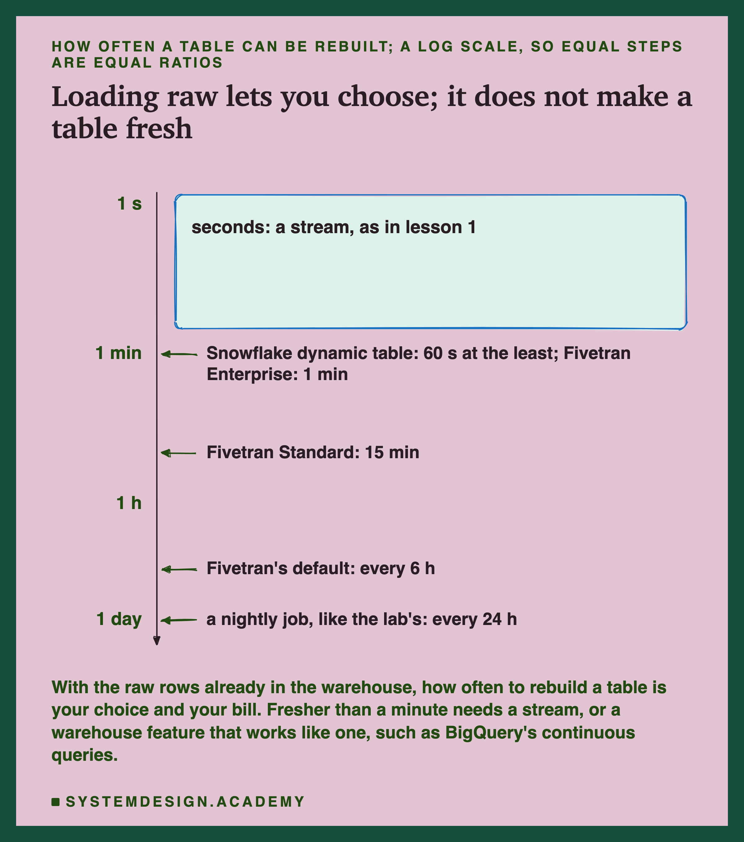
The scale is a log scale, so each labelled step is many times longer than the one above it. A minute is 60 seconds, an hour is 60 minutes, and a day is 24 hours. The vendor marks come from each vendor's own pages; the last mark is simply a nightly job, like the lab's. Fivetran's pricing page lists "15-minute syncs" on its Standard plan and "1-minute syncs" on Enterprise. Its documentation lists settings from 1 minute to 24 hours, with 6 hours as the default. Snowflake's dynamic tables, which refresh themselves to stay within a lag you set, cannot be set below 60 seconds.
The old lesson said you could "wire in change data capture and incremental models for seconds-behind freshness". Change data capture copies each change from a source database as it happens. An incremental model adds only the new rows to a table instead of rebuilding it.
I found nothing to support seconds-behind freshness for dbt and most warehouse transforms, which run on a schedule, and I have cut the claim. One exception I found is BigQuery's continuous queries, which its documentation calls " statements that run continuously". For a number that must be seconds old, you need a stream: a program that never stops and handles each record as it arrives. The first lesson of this chapter measured when that is worth paying for.
Bronze, Silver, Gold
Once raw data is kept and transformed in place, it needs some order, or it turns into a pile nobody trusts. One pattern for this, which Databricks describes, is the medallion pattern, with three layers named bronze, silver and gold. Databricks also calls it a "multi-hop" design, because the data hops from one layer to the next.
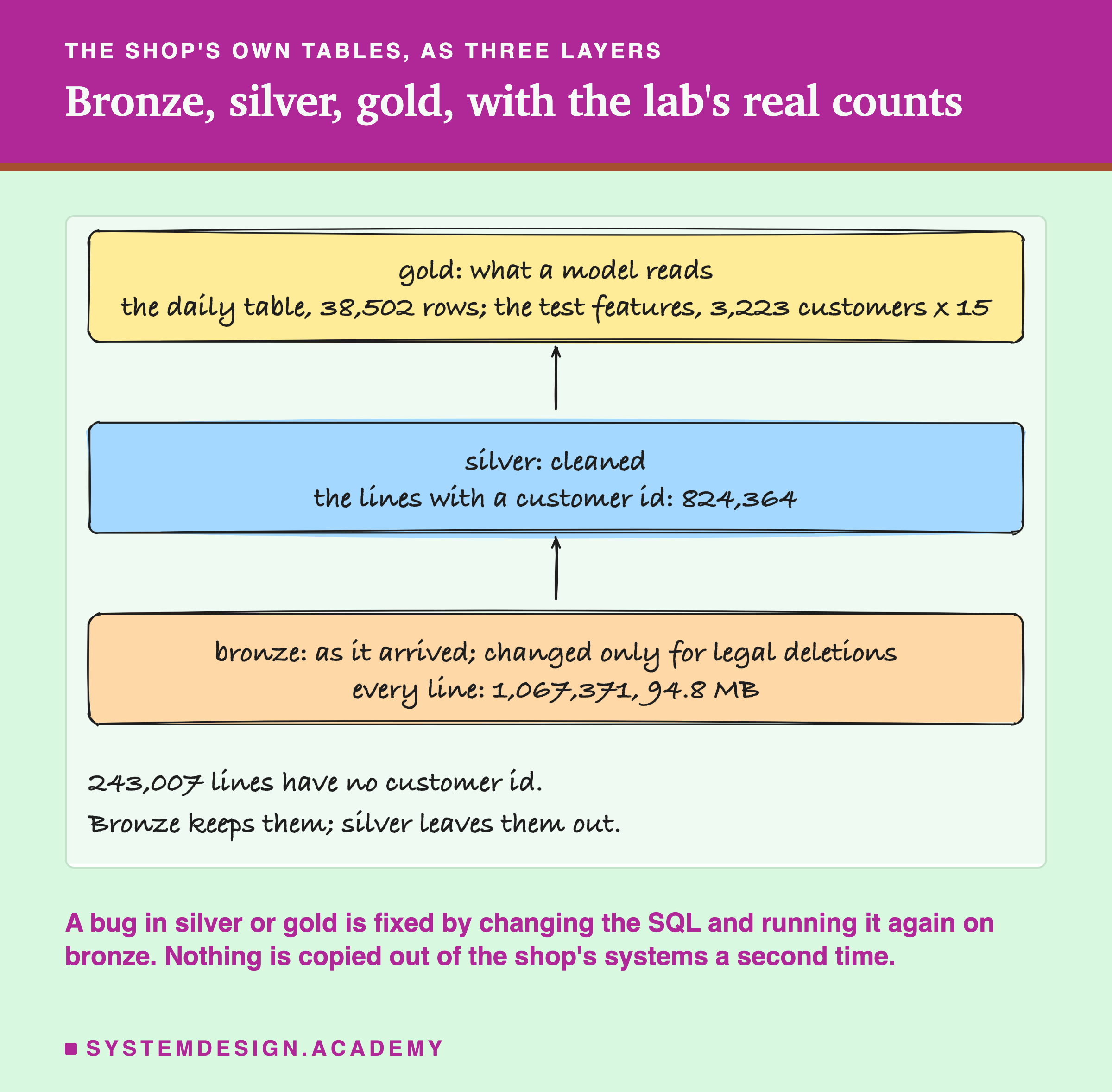
Bronze holds the data exactly as it arrived. In Databricks' words, its tables match the source "'as-is'", plus columns that "capture the load date/time, process ID, etc." Nothing is cleaned and nothing is dropped. Here that is all 1,067,371 lines.
Silver is bronze after cleaning: "matched, merged, conformed and cleansed", which means joined and made consistent. Here the only cleaning is to set aside the 243,007 lines that have no customer id, since no per-customer table can use them. That leaves 824,364 lines.
Gold is the shape a dashboard or a model reads. Here there are two gold tables. One is the daily table, 38,502 rows. The other is the features for the test customers, 3,223 rows of 15 numbers.
Each layer is a set of files that read the layer below. The payoff is repair. If a gold table has a bug, you fix its SQL and run it again on silver and bronze, which a bug fix never touches. Nothing is copied out of the shop's systems a second time. That also means a training table from months ago can be rebuilt, as long as its SQL is pinned to a date, which a later slide covers.
There is one exception to "bronze never changes", and it comes from the law. GDPR gives people a "right to erasure": a company must erase their personal data "without undue delay" when certain grounds apply. It also says personal data may be kept "for no longer than is necessary". So bronze is never edited to fix a bug, but it must allow the deletions the law requires. Raw personal data also needs a set retention period, a rule for how long it is kept before it is deleted.
What the Lab Ran
I wrote the lab's design into the docstring of its script, etl_elt_demo.py, on 30 September 2026, before it ever ran. The script is the same file you can copy from this lesson and run yourself.
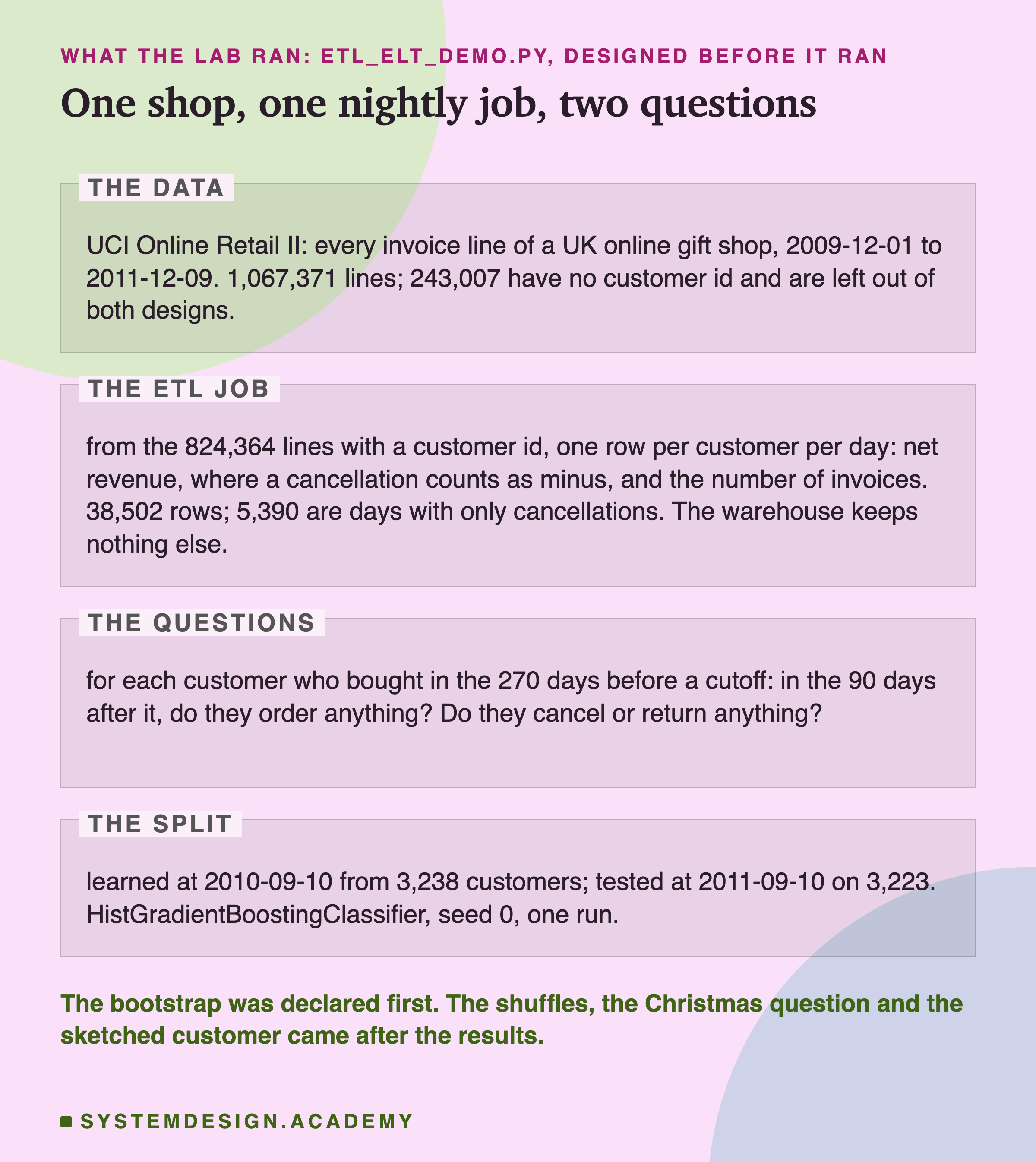
The data is UCI Online Retail II: every invoice line of a UK online shop that sells gifts, from 1 December 2009 to 9 December 2011. Its description says many of the shop's customers are wholesalers, businesses that buy to sell on. Each line is one product on one invoice, with the quantity, the price, the time, the customer id and the country. An invoice number that starts with C is a cancellation. There are 1,067,371 lines. Of these, 243,007 have no customer id, so neither design can use them.
The nightly job is the ETL job. It reads the 824,364 lines that have a customer id, and turns each day's lines into one row per customer per day with two numbers. One is the net revenue: quantity times price, added up, where a cancelled line counts as minus. The other is the number of invoices, orders and cancellations together. The warehouse keeps nothing else. That gives 38,502 rows, and 5,390 of them are days on which the customer only cancelled.
The questions. At a cutoff, take every customer who bought something in the 270 days before it. Then ask two questions about the 90 days after it. Do they order anything? That is buys. Do they cancel or return anything? That is cancels.
The split. The models learn at the cutoff 10 September 2010, from 3,238 customers. They are tested a year later, at the cutoff 10 September 2011, on 3,223 customers. So every test answer is in the future of everything the models learned from.
The Main Run
Here is what the demo stored in results/elt-demo.json. Besides AUC, I report a second score that is easier to picture. Take the tenth of test customers the model was surest about. Top 10% is the share of them who really did the thing.
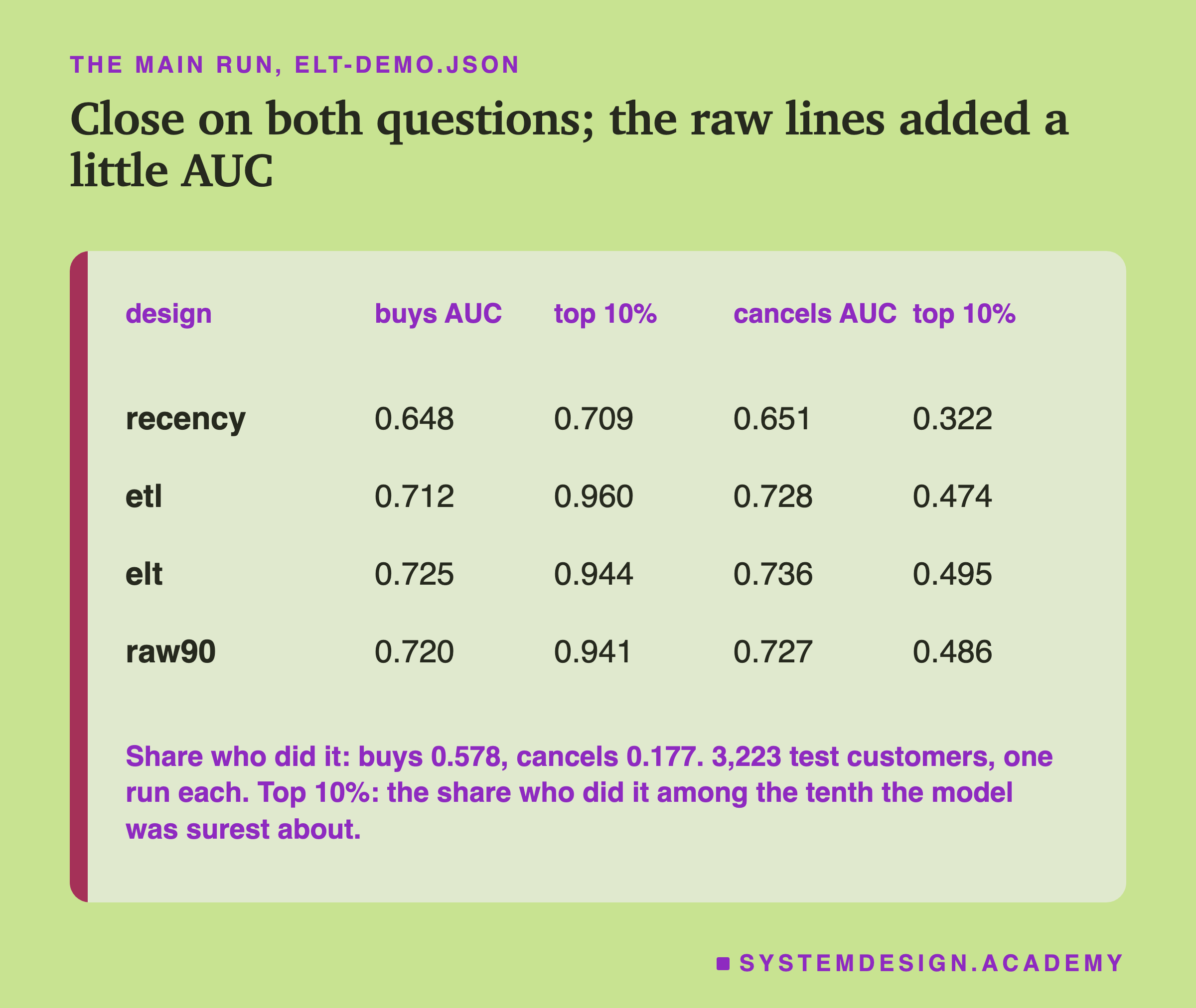
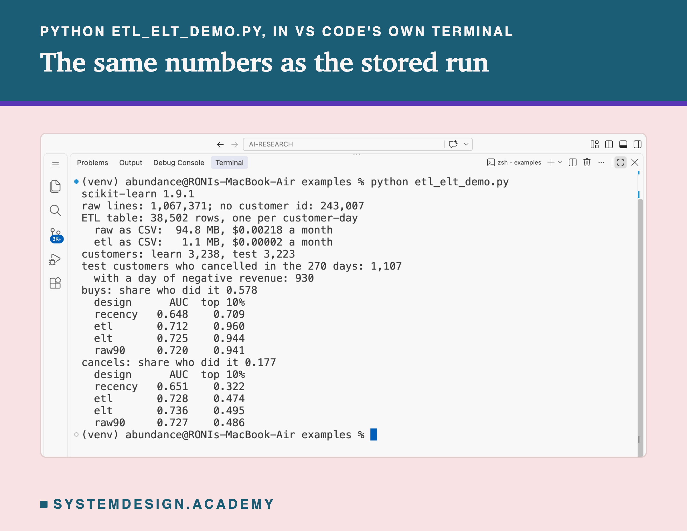
Of the 3,223 test customers, 0.578 ordered again in the 90 days, and 0.177 cancelled something. Days since the last purchase alone gave an AUC of 0.648 for buys and 0.651 for cancels. The eight daily-table features gave 0.712 and 0.728.
Adding the seven raw features gave 0.725 and 0.736. From the unrounded AUCs, those gains are 0.014 for buys and 0.008 for cancels. Both are small. And on the top-10% score for buys, the daily table did better: 0.960 of its surest tenth ordered again, against 0.944 with the raw features.
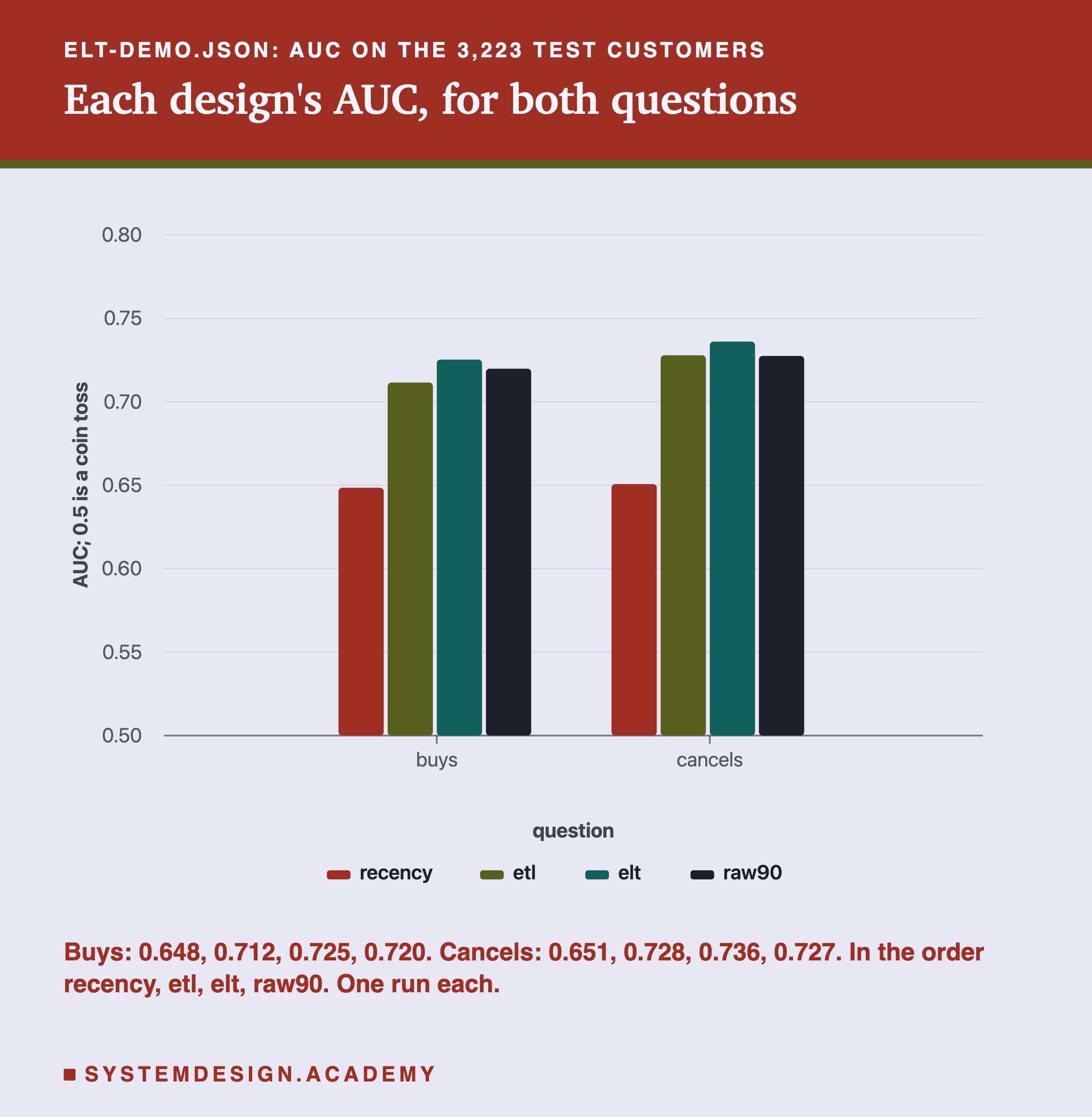
Raw90 landed between the two: 0.720 for buys and 0.727 for cancels. It kept most of the small buys gain and none of the cancels gain. Part of the reason is simple. 1,285 of the 3,223 test customers had no lines at all in the last 90 days before the cutoff, so their seven raw features were blank.
This is not the result the old version of this lesson promised. It said the raw column is the difference between "shipping a model this week and shipping it next quarter". On these two questions, the daily table already held most of what the models could use. The next slides ask whether the small gains are real, where the raw lines did matter, and why.
Could the Gap Be Luck?
A gap of 0.014 on 3,223 customers could come from luck: from which customers happened to be in the test. The demo's design, written before the run, declared one check for this, a bootstrap.
A bootstrap asks: if I had drawn a slightly different test group, how much would the gap move? It picks 3,223 customers from the test group at random, with repeats allowed, and measures the gap on them. Then it does that 1,000 times. The spread of those 1,000 gaps shows how much the gap moves by luck.
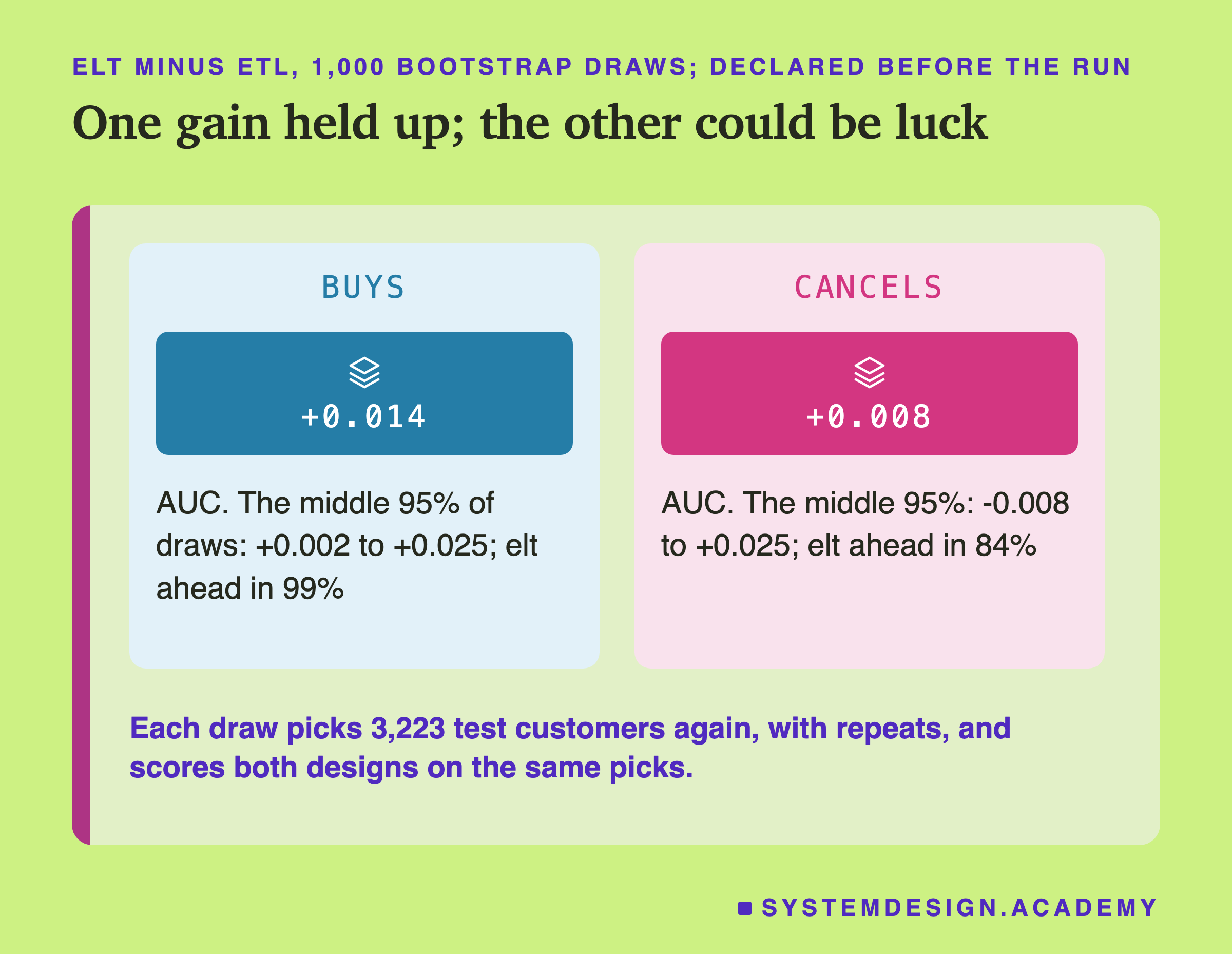
For buys, the middle 95% of the 1,000 gaps ran from +0.002 to +0.025, and elt came out ahead in 99% of them. The gain is small, but here it held up.
For cancels, the middle 95% ran from -0.008 to +0.025. That range includes zero, and elt was ahead in only 84% of draws. So the cancels gain cannot be told apart from luck on this data.
A bootstrap only checks this one question: would a different set of test customers from the same shop and the same year give the same answer? It says nothing about another shop, another year or another model. And one run of one model is one data point.
What the Nightly Job Hid
If the raw lines added so little for cancels, did the daily table see cancellations after all? Partly. When a cancellation outweighs a day's orders, that day's net revenue goes below zero. A negative day is the one sign in the daily table that can only mean a cancellation. The table also counts cancellation invoices in its invoices column, but mixed in with orders. So I counted how many cancellers left a negative day.
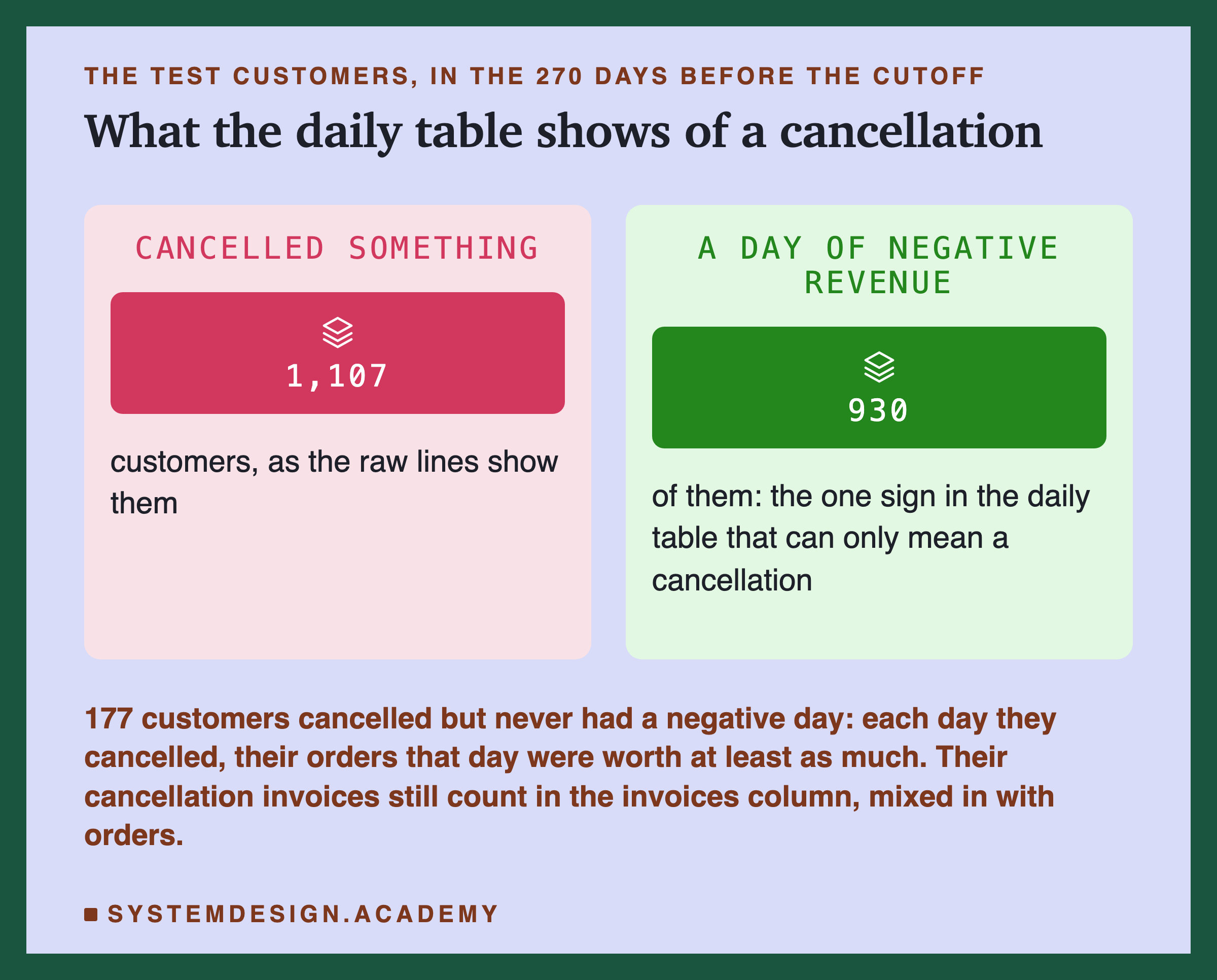
In the 270 days before the test cutoff, 1,107 test customers cancelled at least one line. 930 of them had at least one day of negative revenue in the daily table. That leaves 177 who cancelled but never had a negative day. On each day they cancelled, their orders that same day were worth as much or more, so the net never went below zero. Their cancellation invoices are still in the invoices column, but a reader of the table cannot tell them from orders.
Netting means adding the pluses and the minuses into one total. Here it hid the cancellations of about one canceller in six, and showed the rest only roughly. It could not show how many lines, or what share of invoices, each one cancelled.
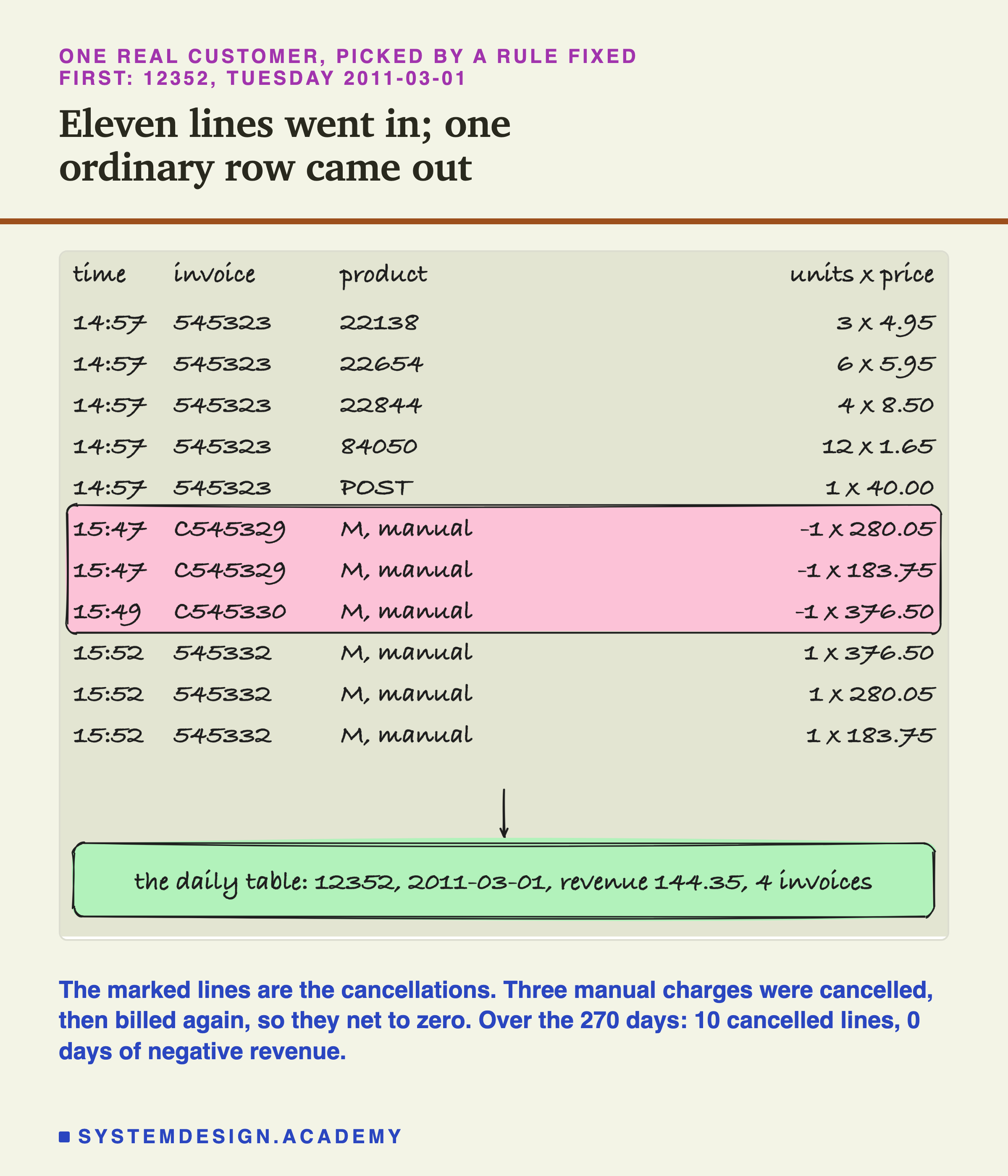
After the results, I picked one customer to look at closely, by a rule fixed before looking at anyone. The rule: the test customer with the lowest id who cancelled at least one line and had no day of negative revenue. That was customer 12352, on Tuesday 1 March 2011.
Which Dropped Column Mattered
Which of the seven raw features did the elt model actually use? After the results, I tested each one by shuffling it. Shuffling a feature mixes its values up across the test customers, so it no longer matches the right person, while its values stay realistic. If the AUC then drops, the model was leaning on that feature.
One shuffle is one random draw, so I shuffled each feature 30 times, with seeds 0 to 29, and kept every result. My first version of this slide used a single shuffle. A review of the lesson ran 30 and showed that a single shuffle can land far from the typical result. So the report now runs 30, and the numbers below come from those.
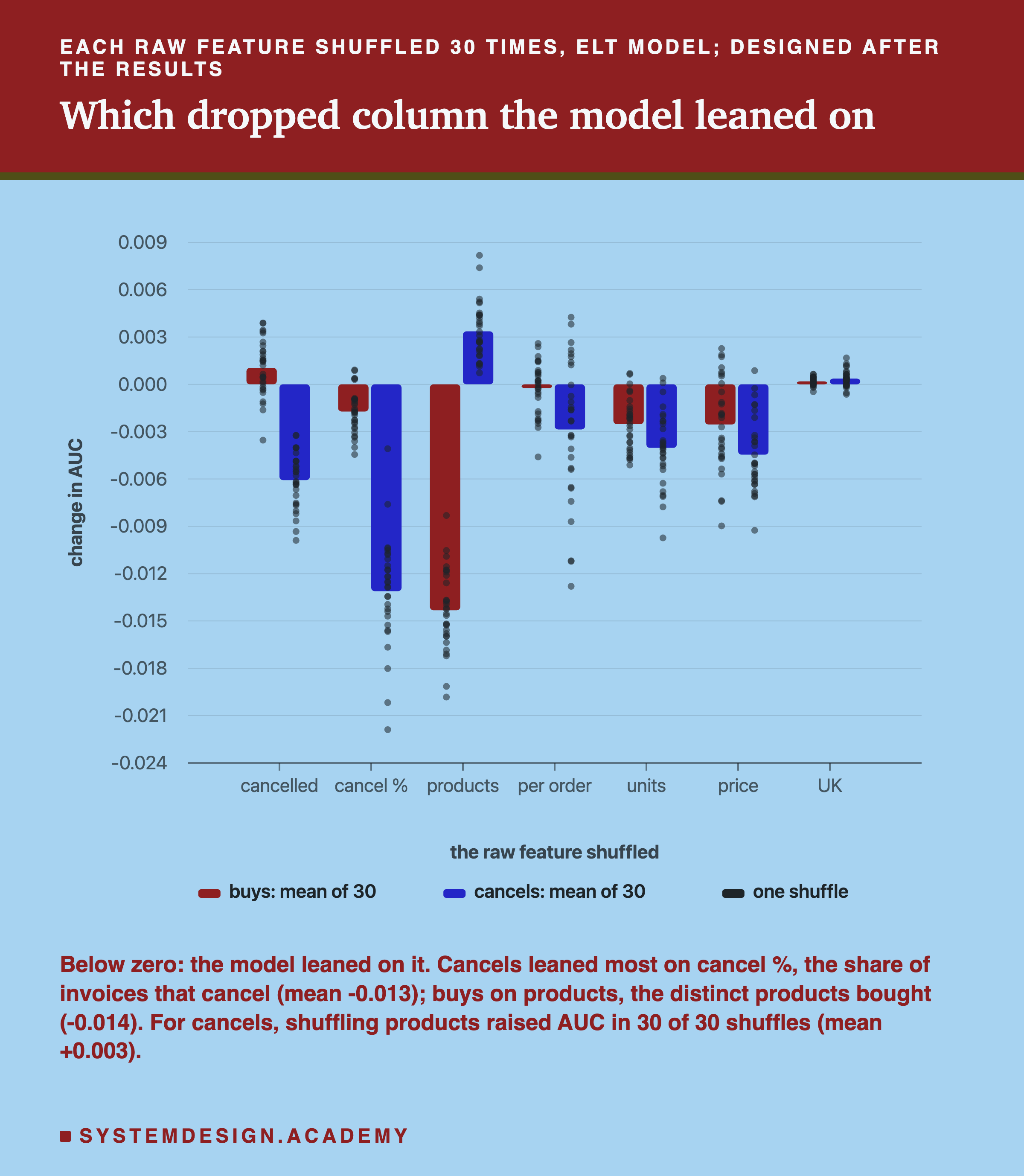
For cancels, the model leaned most on the share of invoices that cancel. Shuffling it lowered the AUC by 0.013 on average, and by between 0.004 and 0.022 in every one of the 30 shuffles. The number of cancelled lines came next, 0.006 on average, also below zero every time. Both features need the raw lines. They are exactly the detail the netting removed.
For buys, the model leaned on the number of different products a customer bought: 0.014 on average, between 0.008 and 0.020, below zero in all 30. Wholesalers tend to buy many products, and this shop sells to many wholesalers, but that is one possible reading, which I did not test. The other raw features moved the buys AUC by 0.003 or less on average, with shuffles on both sides of zero.
One result points the other way, and it is not noise. For cancels, shuffling the number of products raised the AUC in all 30 shuffles, by 0.003 on average and at least 0.001. So the link between products and cancelling that the model learned from the 2010 customers made its 2011 guesses slightly worse. One possible reason, which I did not test, is that this link changed between the two years.
A Question the Table Never Recorded
Buys and cancels are both close to what the daily table holds: money, days and invoices. The real risk of ETL is a question about something the table never recorded at all. So, after seeing the results, I added one such question. I am saying plainly that I chose it knowing the first results were small.
The question: in the 90 days after the cutoff, will the customer order a product whose description contains the word CHRISTMAS? The daily table has no products in it at all.
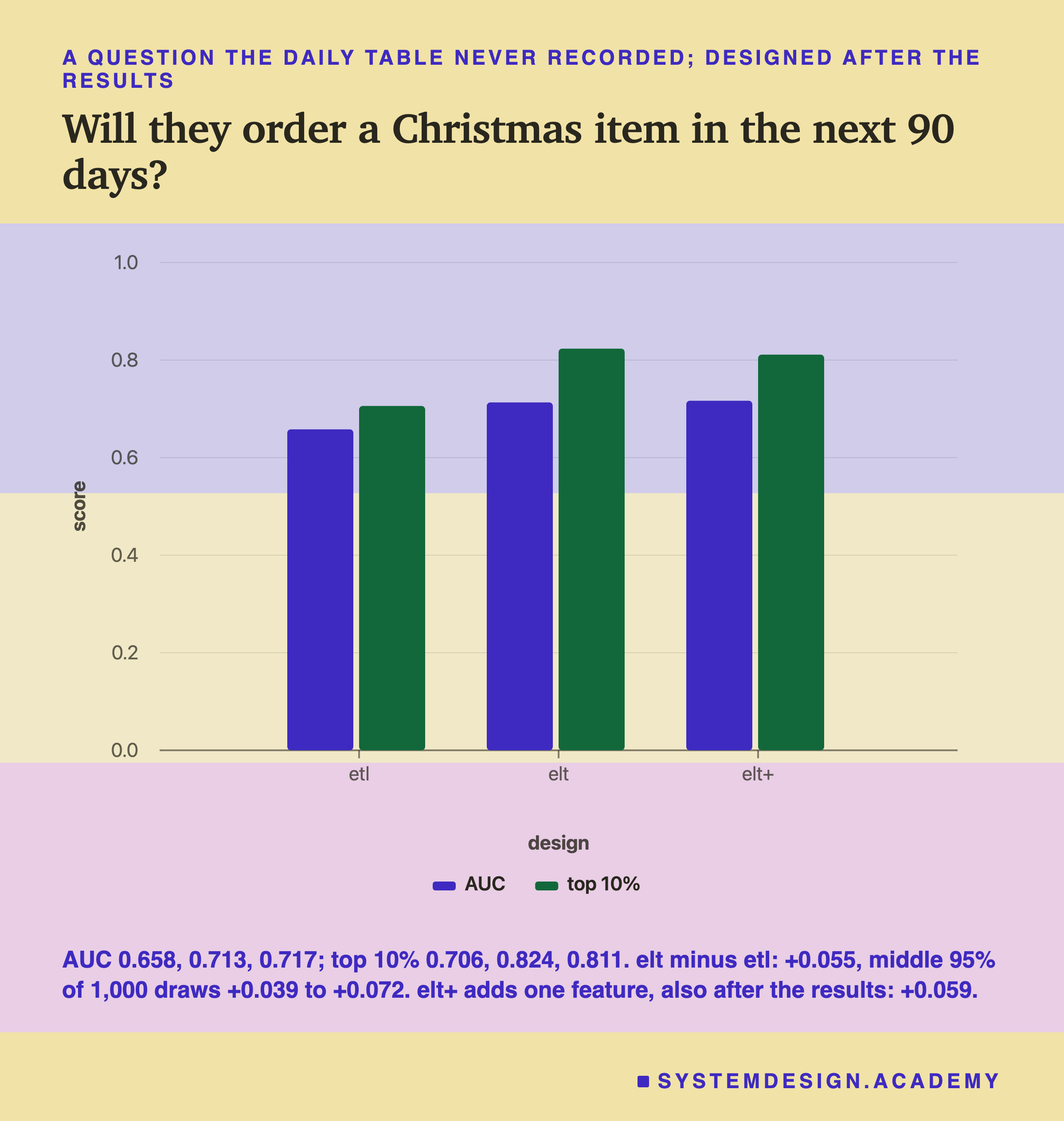
Of the test customers, 0.411 ordered a Christmas item in the 90 days. The daily-table model scored an AUC of 0.658. The elt model, with the same seven raw features as before, scored 0.713, a gain of 0.055. Its surest tenth went from 0.706 who did it to 0.824. Both of those designs were fixed before the first run; only the question came after.
Then I added one feature built for this question: the share of a customer's past lines that were Christmas items. That design, elt+, scored 0.717, only a little more. One possible reason: the 270 days before a September cutoff run from mid-December to early September, so few past lines were Christmas items at all. On average they were 1.2% of a customer's lines.
I ran the same bootstrap as before, 1,000 draws. For elt against etl, the gap of +0.055 had a middle 95% from +0.039 to +0.072. For elt+ against etl, +0.059, from +0.042 to +0.075. So on this question the raw lines added far more than on buys or cancels, and the gain did not look like luck. Keep the order of events in mind, though. I picked this question after seeing that the first two gains were small, and I added the elt+ feature after that.
A Feature Table in dbt, Pinned to a Date
Here is what a transform looks like in an ELT stack. This dbt model builds some of the lab's features in , inside the warehouse. It reads the silver lines and the old daily table, which in ELT is simply one more model.
It is written for Snowflake, from Snowflake's documentation. I have not run it: I have no Snowflake account, and the lab does the same work in pandas.
-- models/gold/customer_features.sql
-- One row per customer, as of a fixed date. Written for Snowflake.
-- Run with: dbt build --vars '{"as_of": "2011-09-10"}'

{{ config(materialized='table', tags=['ml', 'gold']) }}

with lines as (
    select * from {{ ref('stg_lines') }}          -- typed lines with a customer id
    where invoice_day <  '{{ var("as_of") }}'::date
      and invoice_day >= dateadd(day, -270, '{{ var("as_of") }}'::date)
),

days as (
    select * from {{ ref('int_customer_days') }}  -- the old daily table, now a model
    where day <  '{{ var("as_of") }}'::date
      and day >= dateadd(day, -270, '{{ var("as_of") }}'::date)
),

from_days as (
    select
        customer_id,
        datediff(day, max(case when revenue > 0 then day end),
                 '{{ var("as_of") }}'::date)               as recency,
        sum(case when revenue > 0 then 1 else 0 end)       as buy_days,
        sum(revenue)                                       as revenue,
        sum(case when revenue < 0 then 1 else 0 end)       as neg_days
    from days
    group by customer_id
),

from_lines as (
    select
        customer_id,
        sum(case when is_cancel then 1 else 0 end)         as cancel_lines,
        count(distinct case when is_cancel then invoice end)
          / count(distinct invoice)                        as cancel_share,
        count(distinct case when not is_cancel then stock_code end) as products,
        median(case when not is_cancel then unit_price end) as median_price
    from lines
    group by customer_id
)

select d.*, l.cancel_lines, l.cancel_share, l.products, l.median_price
from from_days d
left join from_lines l using (customer_id)
where d.buy_days > 0
Two kinds of text in the model belong to dbt, not to SQL. The parts inside {{ }} are filled in by dbt before the query is sent to the warehouse. ref('stg_lines') becomes the real name of that table, and var('as_of') becomes the date passed in. The table names follow the habit in dbt's own guide to structuring a project. stg_ marks a model, which brings in one source table and tidies it; the guide says each source table gets a single staging model. marks an model, a step between staging and the final tables.
Common Mistakes When Teams Move to ELT
ELT removes some old problems and brings some new ones. These are the ones I would check first on any team making the move. They are general lessons from practice, not numbers measured in this lab.
Editing bronze. The whole value of the raw layer is that it never changes. If someone "fixes" a bad row directly in bronze, old tables can no longer be rebuilt the way they were. Fix it in a silver or gold model, and leave bronze as it arrived. The one exception is a deletion the law requires, such as a GDPR erasure request.
Loading a field that must never be stored. "Load everything" is a default, not a rule that beats a law or a card network's rules. A card's security code must not be kept after the payment is approved. A card number may be kept only in a form nobody can read. To mask a value is to hide part of it, for example all but its last four digits. To tokenize it is to swap it for a stand-in code, a token, that only a separate, locked system can turn back into the real value. Remove, mask or tokenize fields like that before they land.
Transforms that read today's date. A model that uses current_date gives a different answer every day. Pin every transform to an as-of date.
A made-up value that looks real. A common way to fill a gap is to give a customer with no orders a days_since_last_order of 999. A model sees 999 as a real, very large number and learns from it as if it were one. A separate has_ordered flag says what you mean.
A null that quietly becomes an answer. If the gap is not filled, the value is null, which means unknown. In , a null compared with 90 is not true. So case when days_since_last_order > 90 then 1 else 0 end gives 0 for a customer who never ordered, with no error. Decide what a null means before any comparison.
Rebuilding everything, forever. A materialized='table' model is, in dbt's words, "rebuilt as a table on each run". That is fine while tables are small. As history grows, models help: they "insert or update records into a table since the last time that model was run".
Lineage: The Graph dbt Draws
Each dbt model names the models it reads, with ref(). From those names dbt builds the full graph of which table depends on which, and runs the models in order. That graph is called lineage: where each table came from.
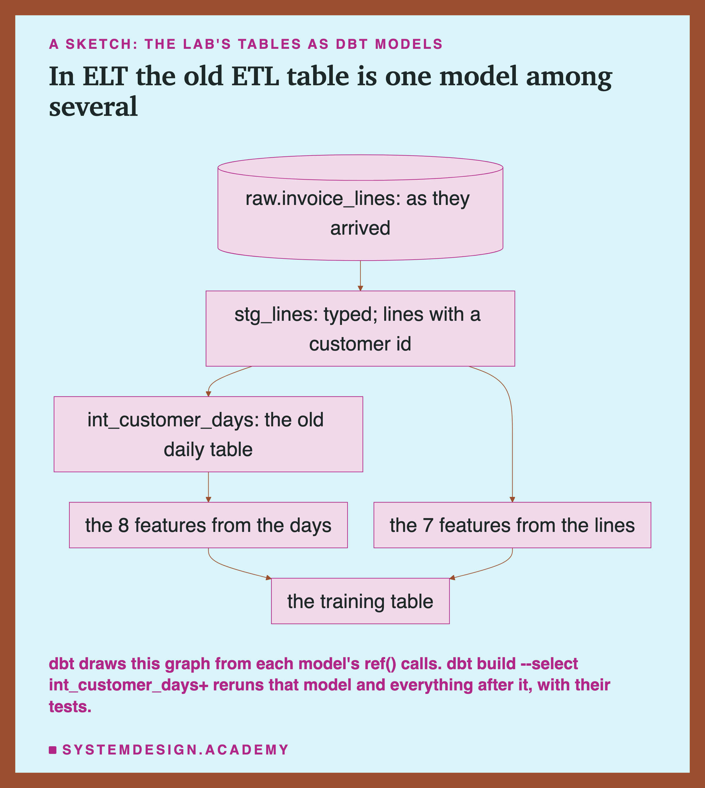
This is a sketch of how the lab's tables would sit in a dbt project. The names are mine, not a real project's. Look at where the old nightly job went. In ELT it is int_customer_days, one model among several, and the seven raw features are a second branch beside it.
The graph gives three things. First, reruns: fix a bug in int_customer_days, and dbt build --select int_customer_days+ reruns it and everything after it. dbt does not do this by itself; the + asks for it. Second, tests: dbt build runs models and tests together, and in dbt's words, "a test failure will cause those downstream resources to skip entirely". Plain dbt run runs no tests. Third, documents: dbt docs generate builds a site with the graph and the descriptions you write for each model and column.
The old version of this lesson said this lineage traces "any feature back to the exact raw source it came from". That made it sound as if every column were traced for free. dbt Core draws lineage between models, not between columns. In dbt's own products, column-level lineage needs its paid Catalog, on its Enterprise plans, or its newer v2 edition, which is not fully open source.
When ETL Still Wins
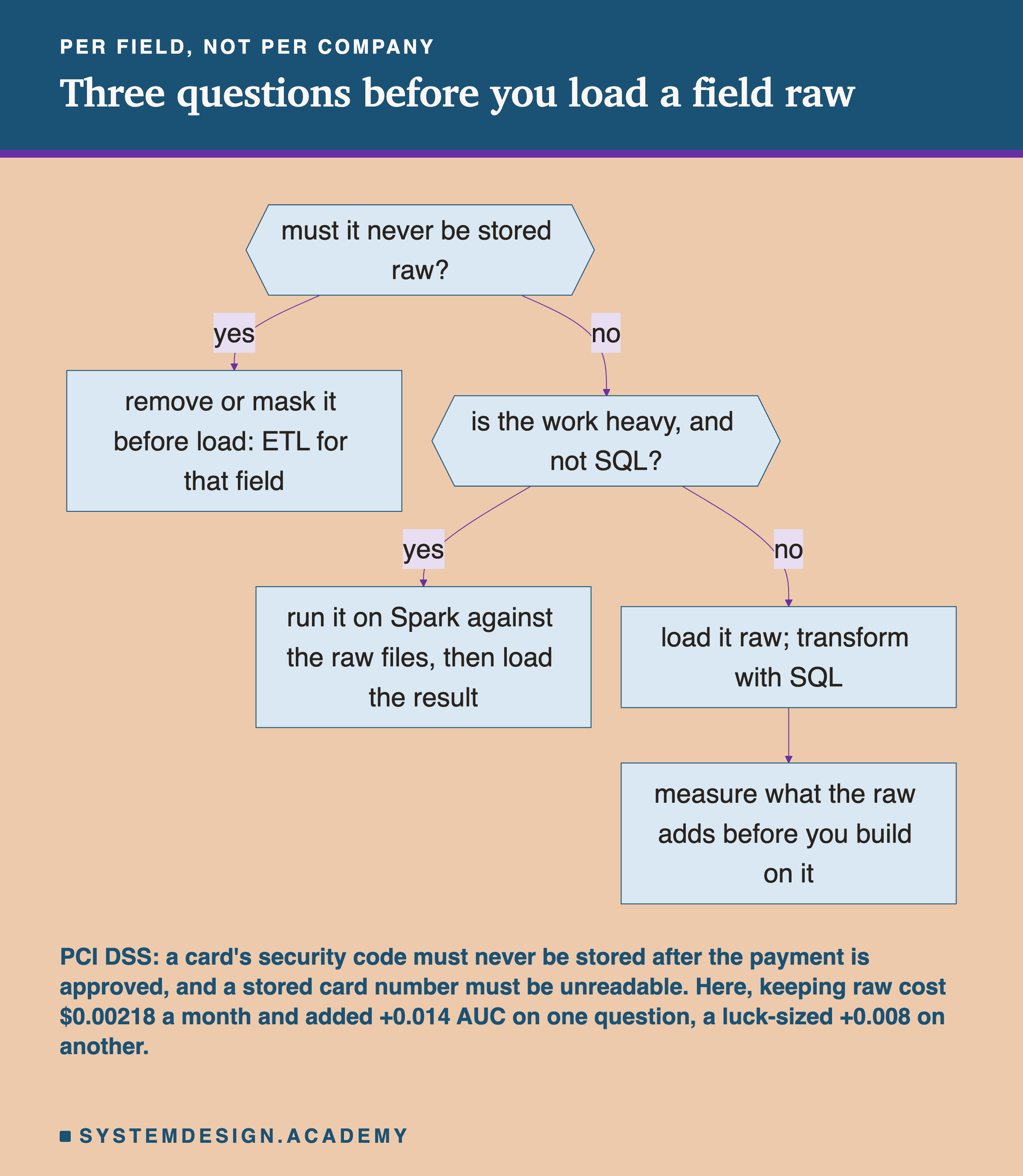
ELT is a common default, not a law. There are real cases where transforming first is right. The question is best asked for each field, not for the whole company.
| Situation | Order | Why |
|---|---|---|
| Normal cleaning, joins and sums in a warehouse | ELT | Cheap in place, raw history kept, tables can be rebuilt |
| A field that must never be stored raw | ETL for that field | Remove or mask it before it lands |
| Heavy work that is not SQL, such as images or audio | ETL or a mix | Run it on Spark, then load the result |
| No warehouse that can run transforms cheaply | ETL | Transforming in place would cost too much |
The sharpest case is a field that must never be stored. The old lesson said GDPR or HIPAA may forbid "ever storing raw personal data, even briefly". Neither law says that. GDPR, the EU's data protection law, says personal data must be "adequate, relevant and limited to what is necessary". It names safeguards such as "pseudonymisation", replacing a name with a code. HIPAA, a US health privacy law, "requires appropriate administrative, physical and technical safeguards".
How Real Teams Describe It
The usual account of why ELT spread is that two costs fell: storing raw data got cheap, and warehouse compute split away from storage. Here are the dated facts behind that account, each from the company's own release, filing, post or code history.
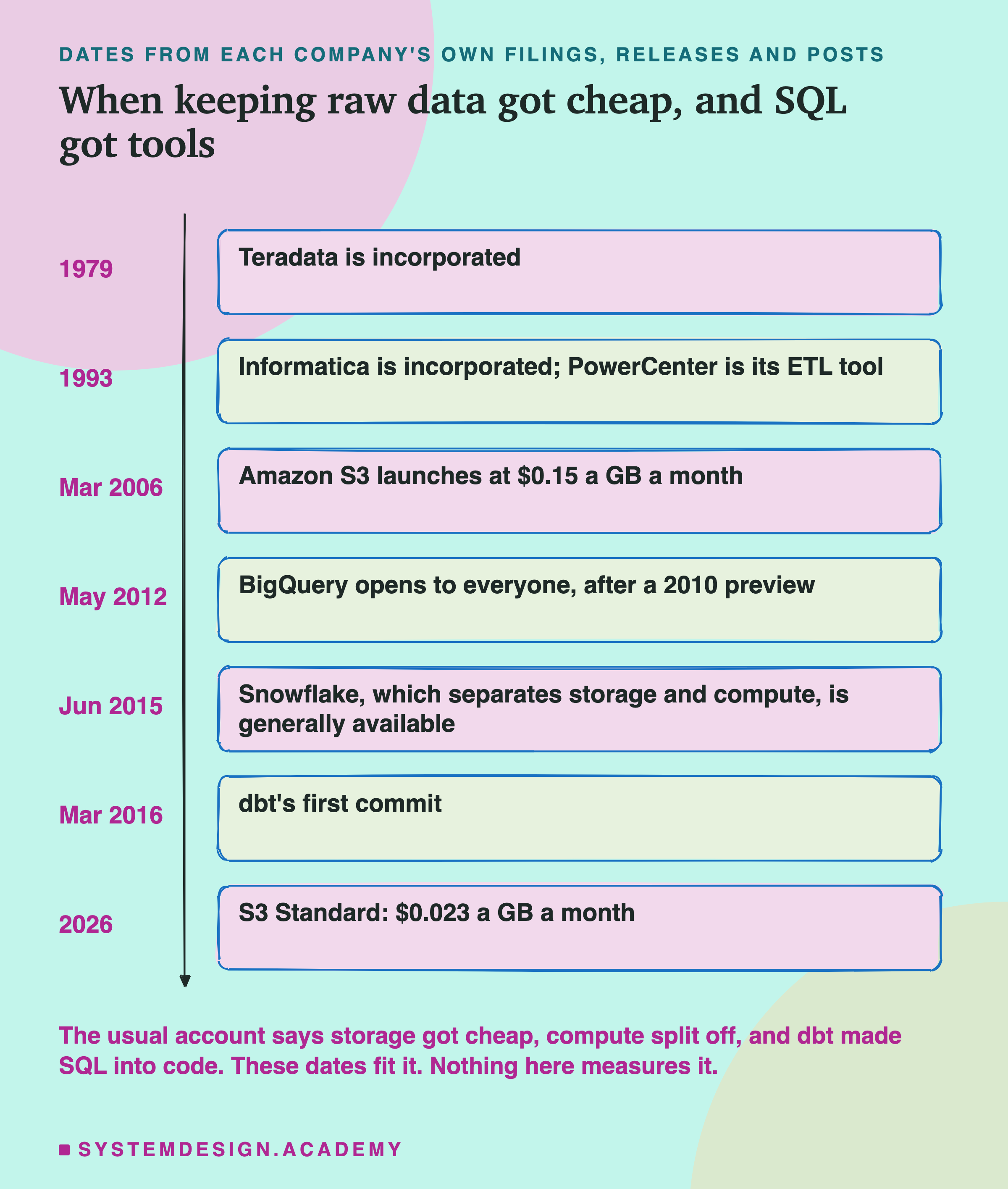
Amazon S3 launched on 14 March 2006 at $0.15 per GB a month; its Standard storage lists $0.023 today. BigQuery was shown to a few developers in May 2010 and opened to everyone on 1 May 2012. Snowflake was incorporated in July 2012 and has been "generally available since June 2015". dbt's first commit is dated 10 March 2016. The old version of this lesson put cheap S3 at "~2012" and the warehouse split at "2014-2016". Both were wrong, and the StepDiagram below now has the right dates.
The old lesson also said that Spotify and DoorDash "run warehouse-centric ELT with dbt for the bulk of their analytics and ML feature work". I could not find either company saying that in its own words, so I have cut it. Three companies do describe loading raw first and then transforming with dbt, in their own posts.
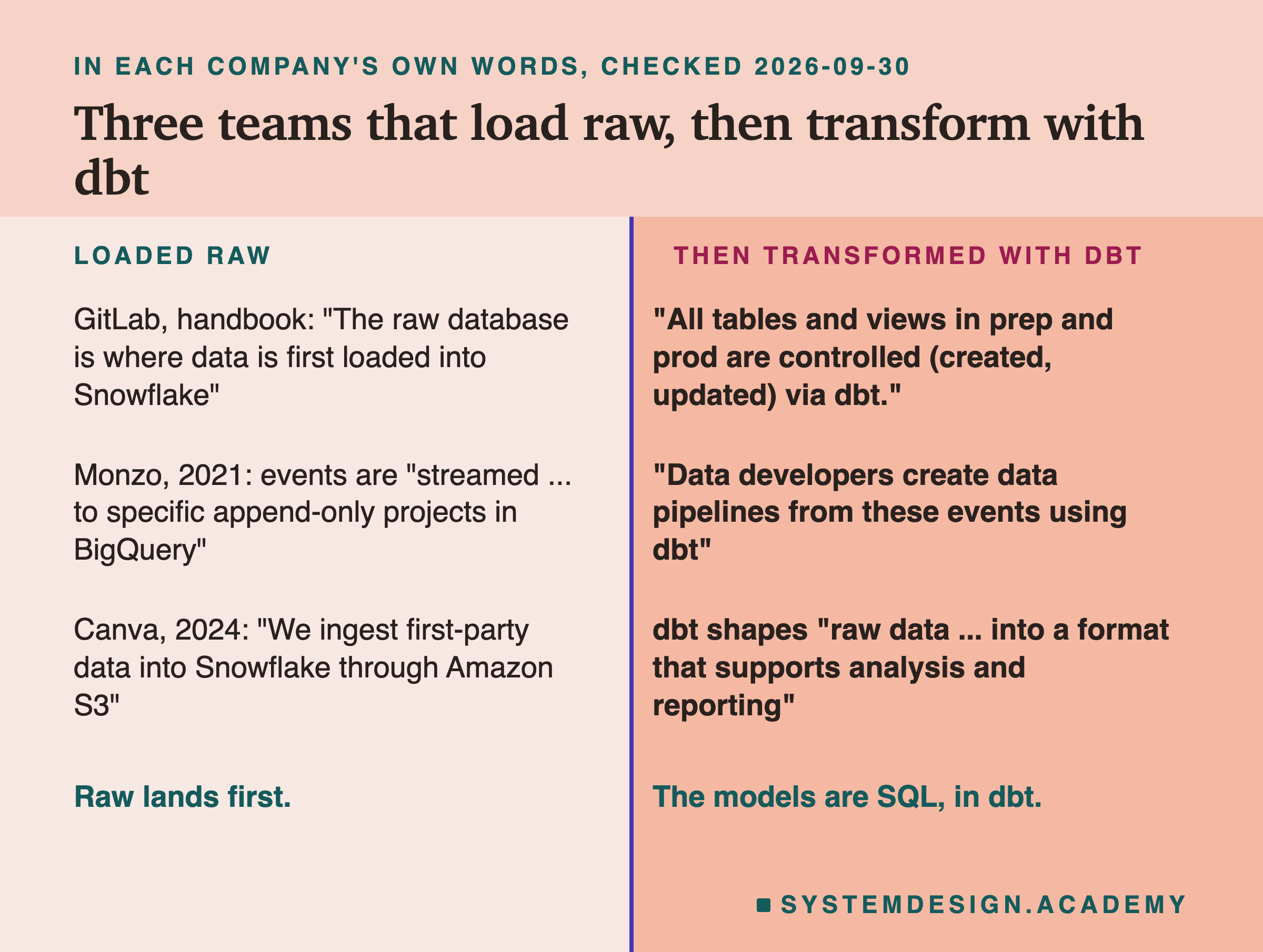
GitLab keeps its data team's handbook in public. It says tools such as Stitch and Fivetran move data "into our Snowflake ". It also says "the raw database is where data is first loaded into Snowflake". And it says "all tables and views in prep and prod are controlled (created, updated) via dbt".
Try It Yourself
This script is the lab. It downloads the shop's data and builds the nightly daily table. It computes the 8 daily-table features and the 7 raw features at both cutoffs, and trains the four designs for both questions. It prints each design's AUC and top-10% score, plus the sizes and the cancellations the daily table missed. It needs no GPU. When I ran it on an idle laptop, it finished in about 9 seconds once the data was downloaded. It takes longer when the machine is busy.
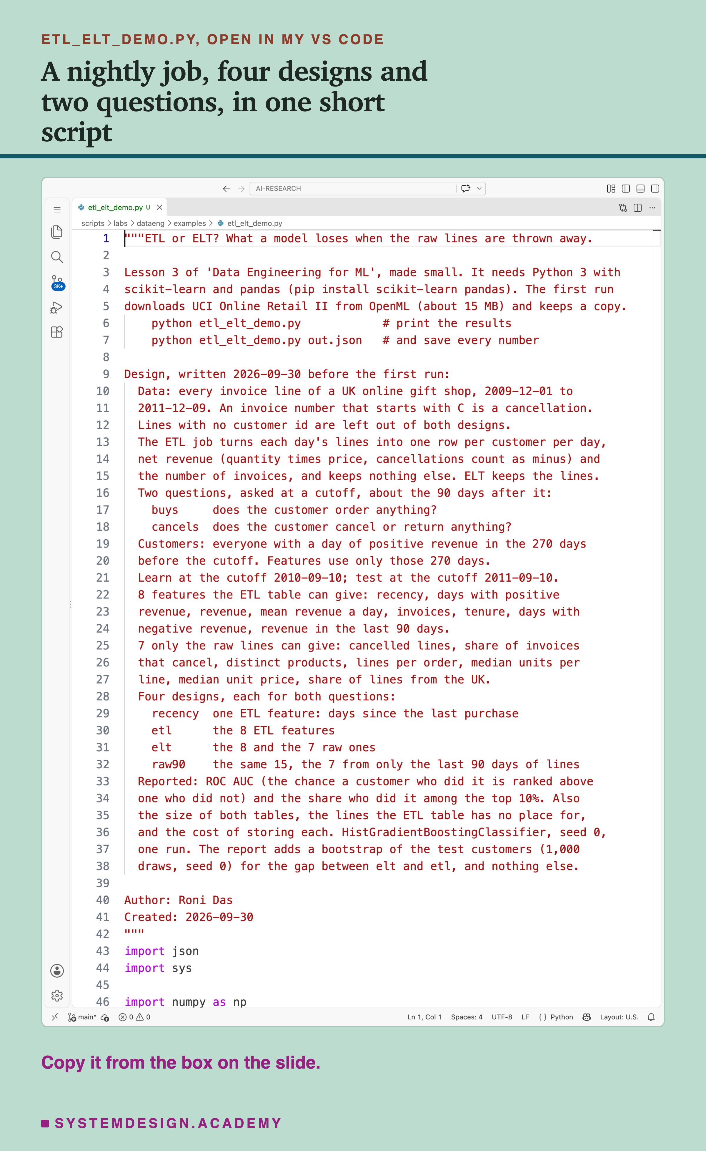
Before you run this lab. You need Python 3 and two libraries: pip install scikit-learn pandas. scikit-learn holds the model and the download, and brings NumPy with it; pandas holds the tables. The first run downloads Online Retail II from OpenML (about 15 MB), so it needs an internet connection once. After that, scikit-learn keeps a copy in a folder in your home directory (scikit_learn_data).
I ran it with scikit-learn 1.9.1 on a Mac. scikit-learn runs the same way on Windows and Linux, but I have not checked the numbers there. Another version of scikit-learn may give different decimals, so the first line printed is the version. Give it a file name, python etl_elt_demo.py out.json, and it also saves every number at full precision; that is how results/elt-demo.json was made.
"""ETL or ELT? What a model loses when the raw lines are thrown away.

Lesson 3 of 'Data Engineering for ML', made small. It needs Python 3 with
scikit-learn and pandas (pip install scikit-learn pandas). The first run
downloads UCI Online Retail II from OpenML (about 15 MB) and keeps a copy.
    python etl_elt_demo.py            # print the results
    python etl_elt_demo.py out.json   # and save every number

Design, written 2026-09-30 before the first run:
  Data: every invoice line of a UK online gift shop, 2009-12-01 to
  2011-12-09. An invoice number that starts with C is a cancellation.
  Lines with no customer id are left out of both designs.
  The ETL job turns each day's lines into one row per customer per day,
  net revenue (quantity times price, cancellations count as minus) and
  the number of invoices, and keeps nothing else. ELT keeps the lines.
  Two questions, asked at a cutoff, about the 90 days after it:
    buys     does the customer order anything?
    cancels  does the customer cancel or return anything?
  Customers: everyone with a day of positive revenue in the 270 days
  before the cutoff. Features use only those 270 days.
  Learn at the cutoff 2010-09-10; test at the cutoff 2011-09-10.
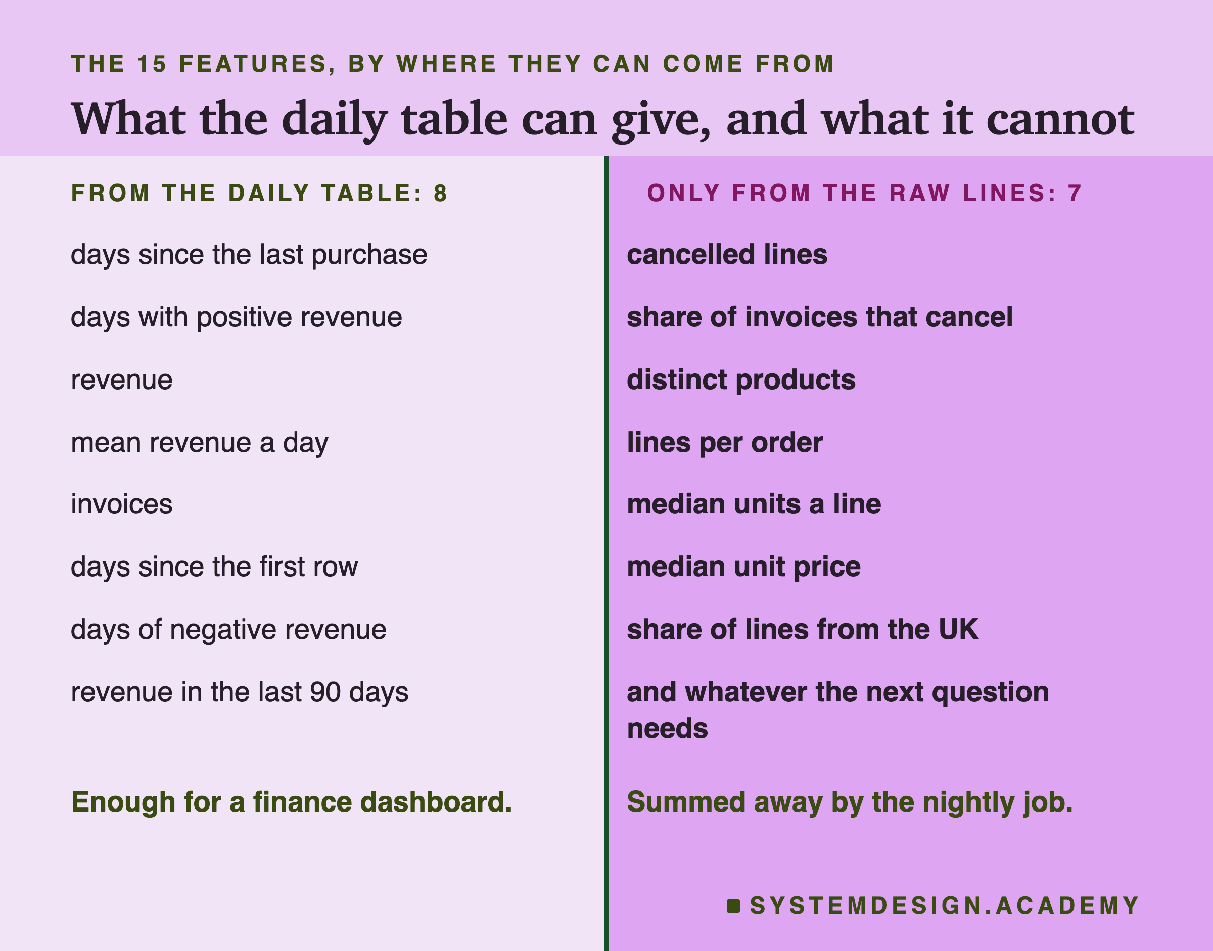
  8 features the ETL table can give: recency, days with positive
  revenue, revenue, mean revenue a day, invoices, tenure, days with
  negative revenue, revenue in the last 90 days.
  7 only the raw lines can give: cancelled lines, share of invoices
  that cancel, distinct products, lines per order, median units per
  line, median unit price, share of lines from the UK.
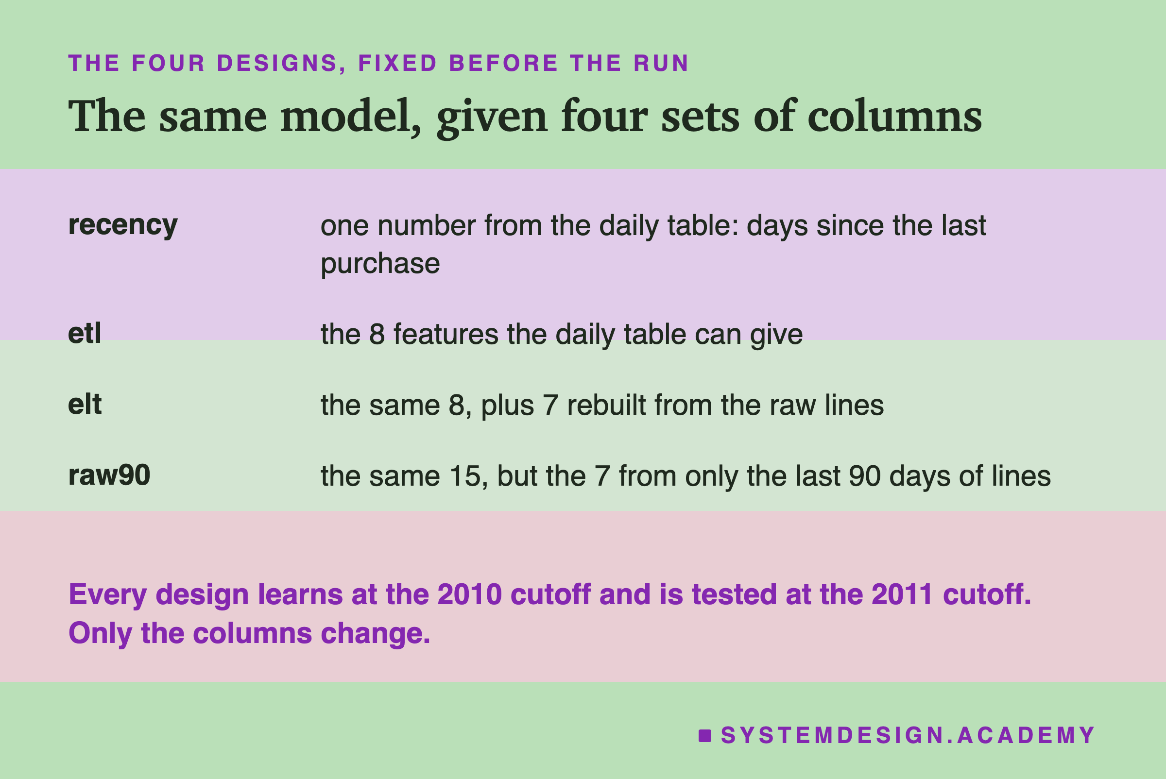
  Four designs, each for both questions:
    recency  one ETL feature: days since the last purchase
    etl      the 8 ETL features
    elt      the 8 and the 7 raw ones
    raw90    the same 15, the 7 from only the last 90 days of lines
  Reported: ROC AUC (the chance a customer who did it is ranked above
  one who did not) and the share who did it among the top 10%. Also
  the size of both tables, the lines the ETL table has no place for,
  and the cost of storing each. HistGradientBoostingClassifier, seed 0,
  one run. The report adds a bootstrap of the test customers (1,000
  draws, seed 0) for the gap between elt and etl, and nothing else.

Author: Roni Das
Created: 2026-09-30
"""
import json
import sys

import numpy as np
import pandas as pd
import sklearn
from sklearn.datasets import fetch_openml
from sklearn.ensemble import HistGradientBoostingClassifier
from sklearn.metrics import roc_auc_score

S3_PRICE = 0.023  # US dollars per GB a month, S3 Standard, first 50 TB
DAY = pd.Timedelta(days=1)

raw = fetch_openml(data_id=43368, as_frame=True, parser="auto").frame
raw_bytes = len(raw.to_csv(index=False).encode())
raw["when"] = pd.to_datetime(raw["InvoiceDate"])
raw["day"] = raw["when"].dt.normalize()
raw["cancel"] = raw["Invoice"].str.startswith("C")
# prices have at most 3 decimals, so money is summed exactly, in 1/1000 GBP
raw["milli"] = (raw["Price"] * 1000).round().astype("int64") * raw["Quantity"]
lines = raw[raw["Customer_ID"].notna()]

# The ETL job: one row per customer per day. Nothing else is kept.
etl = (lines.groupby(["Customer_ID", "day"])
       .agg(milli=("milli", "sum"), invoices=("Invoice", "nunique"))
       .reset_index())
etl_bytes = len(etl.assign(revenue=etl["milli"] / 1000)
                .drop(columns="milli").to_csv(index=False).encode())


def from_etl(T):
    """The 8 features, from the ETL table only, for the 270 days before T."""
    e = etl[(etl["day"] >= T - 270 * DAY) & (etl["day"] < T)]
    g, buy = e.groupby("Customer_ID"), e[e["milli"] > 0].groupby("Customer_ID")
    f = pd.DataFrame({"recency": (T - buy["day"].max()).dt.days})
    f["buy_days"] = buy.size()
    f["revenue"] = g["milli"].sum()
    f["per_day"] = g["milli"].sum() / g.size()
    f["invoices"] = g["invoices"].sum()
    f["tenure"] = (T - g["day"].min()).dt.days
    f["neg_days"] = e[e["milli"] < 0].groupby("Customer_ID").size()
    f["last_90"] = e[e["day"] >= T - 90 * DAY].groupby("Customer_ID")["milli"].sum()
    return f.fillna({"neg_days": 0, "last_90": 0})


def from_raw(T, days, who):
    """The 7 features only the raw lines can give, for `days` before T."""
    r = lines[(lines["day"] >= T - days * DAY) & (lines["day"] < T)]
    sale, gone = r[~r["cancel"]], r[r["cancel"]]
    by, s = r.groupby("Customer_ID"), sale.groupby("Customer_ID")
    f = pd.DataFrame({"cancel_lines": gone.groupby("Customer_ID").size()},
                     index=by.size().index).fillna(0)
    f["cancel_share"] = gone.groupby("Customer_ID")["Invoice"].nunique()
    f["cancel_share"] = f["cancel_share"].fillna(0) / by["Invoice"].nunique()
    f["products"] = s["StockCode"].nunique()
    f["per_order"] = s.size() / s["Invoice"].nunique()
    f["units"] = s["Quantity"].median()
    f["price"] = s["Price"].median()
    f["uk"] = (r["Country"] == "United Kingdom").groupby(r["Customer_ID"]).mean()
    return f.reindex(who)  # a customer with no lines in the window: blank


def cohort(cutoff):
    T = pd.Timestamp(cutoff)
    X = from_etl(T)
    later = lines[(lines["day"] >= T) & (lines["day"] < T + 90 * DAY)]
    y = {"buys": X.index.isin(later.loc[~later["cancel"], "Customer_ID"]),
         "cancels": X.index.isin(later.loc[later["cancel"], "Customer_ID"])}
    tables = {"recency": X[["recency"]], "etl": X,
              "elt": X.join(from_raw(T, 270, X.index)),
              "raw90": X.join(from_raw(T, 90, X.index))}
    return tables, y


def top10(y, p):
    order = np.argsort(-p, kind="stable")[:int(np.ceil(0.1 * len(y)))]
    return float(y[order].mean())


learn, y_learn = cohort("2010-09-10")
test, y_test = cohort("2011-09-10")
n_raw, n_cust = len(raw), len(lines)
out = {"scikit_learn": sklearn.__version__, "raw_lines": n_raw,
       "no_customer_id": n_raw - n_cust, "etl_rows": len(etl),
       "raw_bytes": raw_bytes, "etl_bytes": etl_bytes,
       "learn_customers": len(y_learn["buys"]),
       "test_customers": len(y_test["buys"])}
print(f"scikit-learn {sklearn.__version__}")
print(f"raw lines: {n_raw:,}; no customer id: {n_raw - n_cust:,}")
print(f"ETL table: {len(etl):,} rows, one per customer-day")
for k in ("raw", "etl"):
    mb = out[f"{k}_bytes"] / 1e6
    out[f"{k}_dollars_a_month"] = mb / 1000 * S3_PRICE
    print(f"  {k} as CSV: {mb:5.1f} MB, ${mb / 1000 * S3_PRICE:.5f} a month")
print(f"customers: learn {out['learn_customers']:,}, "
      f"test {out['test_customers']:,}")

# What the netting hid: cancellations that leave no negative day behind.
t = test["elt"]
out["test_cancelled_before"] = int((t["cancel_lines"] > 0).sum())
out["of_them_negative_day"] = int(((t["cancel_lines"] > 0)
                                   & (t["neg_days"] > 0)).sum())
print(f"test customers who cancelled in the 270 days: "
      f"{out['test_cancelled_before']:,}")
print(f"  with a day of negative revenue: {out['of_them_negative_day']:,}")

out["results"] = {}
for q in ("buys", "cancels"):
    out["results"][q] = {"share": float(y_test[q].mean())}
    print(f"{q}: share who did it {y_test[q].mean():.3f}")
    print(f"  {'design':<8} {'AUC':>6} {'top 10%':>8}")
    for d in ("recency", "etl", "elt", "raw90"):
        model = HistGradientBoostingClassifier(random_state=0)
        model.fit(learn[d], y_learn[q])
        p = model.predict_proba(test[d])[:, 1]
        auc, top = float(roc_auc_score(y_test[q], p)), top10(y_test[q], p)
        out["results"][q][d] = {"auc": auc, "top10": top}
        print(f"  {d:<8} {auc:6.3f} {top:8.3f}")

if len(sys.argv) > 1:  # a file name was given: save every number too
    json.dump(out, open(sys.argv[1], "w"), indent=1)
The Lab Report
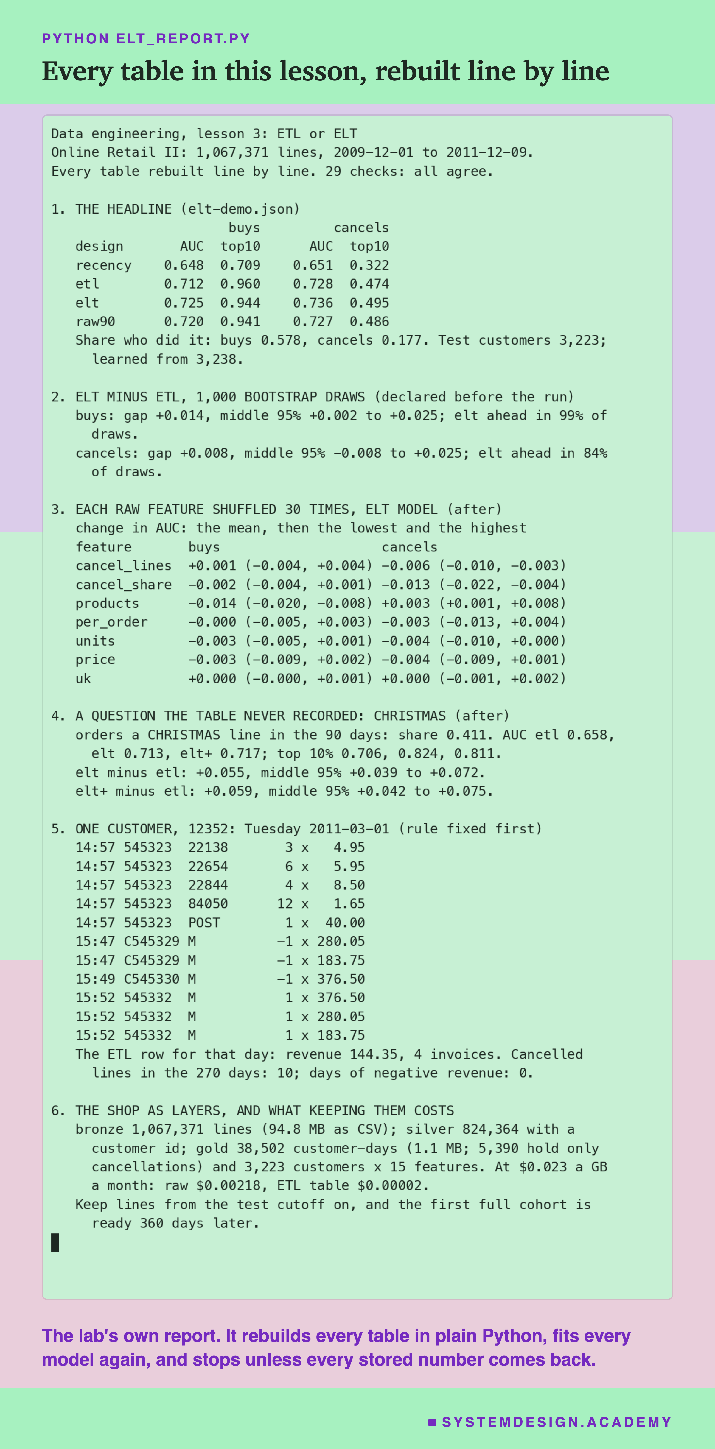
The report lives in scripts/labs/dataeng/elt_report.py. It reads the demo's stored files, results/elt-demo.json and the printed run, and the shop's data from scikit-learn's local copy. It does not trust the demo's arithmetic. The demo builds its tables with pandas. The report walks the 824,364 lines one at a time in plain Python, with dictionaries and sets, and builds the daily table and all 15 features again.
Then it fits every model again on its own tables. It also writes its own daily table out as CSV and measures it, so the 1.1 MB is checked too. It stops unless every stored count, size and AUC comes back exactly. All 29 checks agreed. It changes nothing in the demo's files.
Its json mode writes every number to results/elt-report.json, which the figures read. The demo mode checks the demo's printed run line by line. The box mode writes the playground on the next slide and checks it against both files.
Rank the Customers Yourself, No Model
This box has no model in it. It holds all 3,223 test customers, in order. For each one it has the two answers: did they order in the 90 days, and did they cancel? It also has the etl and elt models' scores for both questions, rounded to a thousandth. And it has two counts: cancelled lines, which only the raw lines have, and days of negative revenue, which the daily table shows. Each number is stored as characters in base 64, which just means counting with 64 different digits instead of 10, so that the box stays small. It runs in your browser.
The answers and the two counts are exact. The scores are rounded, so the box's AUC can differ from the stored one in the fourth decimal. The report checked that every box AUC is within 0.002 of the stored one; the largest difference was 0.00005. Because of that rounding, the box prints 0.711 for etl on buys, where the stored AUC rounds to 0.712.
As it is, the box prints each design's AUC and top-10% score for both questions. Then it ranks customers for the cancels question by one count, with no model at all. Ranking by cancelled lines, which only the raw lines have, gives an AUC of 0.709. Ranking by days of negative revenue, the daily table's trace, gives 0.680.
So a single raw count, on its own, ranked cancellers better than the daily table's best clue. Yet the elt model, with all 15 features, beat the etl model by only 0.008. One possible reading, which I did not test: the eight daily features already carry much of what the count knows, such as how often a customer orders.
Then try top10(CANCELLED, DID['cancels']) for the count's top-10% score. Try auc(SCORE[('buys', 'elt')], DID['cancels']), a buys model asked the cancels question. Ask yourself which of these you could have measured without the raw lines.
Working One Customer Out by Hand
Before you trust a transform, I think you should be able to compute its output with a pencil. So here is customer 12352's day, Tuesday 1 March 2011, turned into its row in the daily table by hand.
The first invoice, 545323 at 14:57, has five lines. 3 times 4.95 is 14.85. 6 times 5.95 is 35.70. 4 times 8.50 is 34.00. 12 times 1.65 is 19.80. Postage is 1 times 40.00. Those add up to 144.35.
The next two invoices are cancellations. C545329 has two manual lines, minus 280.05 and minus 183.75. C545330 has one, minus 376.50. The last invoice, 545332, bills the same three amounts again, plus 376.50, plus 280.05 and plus 183.75. The three minuses and the three pluses add up to exactly zero.
So the day's net revenue is 144.35 plus zero, which is 144.35. The day had four invoices: 545323, C545329, C545330 and 545332. That gives the daily table's row: customer 12352, 1 March 2011, revenue 144.35, 4 invoices. The report printed exactly that.
Now the raw features. Over the 270 days, this customer had 8 invoices. 3 of them were cancellations, so the share of invoices that cancel is 3 divided by 8, which is 0.375. They cancelled 10 lines in all. The 8 invoices can be counted from the daily table, by adding up its invoice column. But the share and the cancelled lines cannot: each row holds one sum and one count, and the table does not say which of the invoices cancelled.
Map the pencil work onto the dbt model on the slide "A Feature Table in dbt, Pinned to a Date". sum(revenue) over the days is the addition. count(distinct case when is_cancel then invoice end) / count(distinct invoice) is 3 divided by 8. The warehouse does the same arithmetic for every customer at once.
The Code, Part by Part
Loading. fetch_openml(data_id=43368) downloads Online Retail II once and reads the local copy after that. raw_bytes measures the whole table as CSV, before anything is added to it. milli is quantity times price in thousandths of a pound, as whole numbers. The prices have at most three decimals, so every sum is exact. lines keeps only the lines with a customer id.
The ETL job. One groupby over customer and day, with two numbers: the sum of milli and the count of distinct invoices. That table, etl, is all the nightly job keeps. etl_bytes measures it as CSV.
from_etl(T). The 8 features, from the daily table only, for the 270 days before the cutoff T. Customers with no day of positive revenue in those days are left out, so every customer in a cohort bought something.
from_raw(T, days, who). The 7 features that need the lines, for the days before T. sale and split the lines into orders and cancellations. A customer with no lines in the window gets blanks, and the model handles blanks by itself.
How to Keep Raw Data, Step by Step
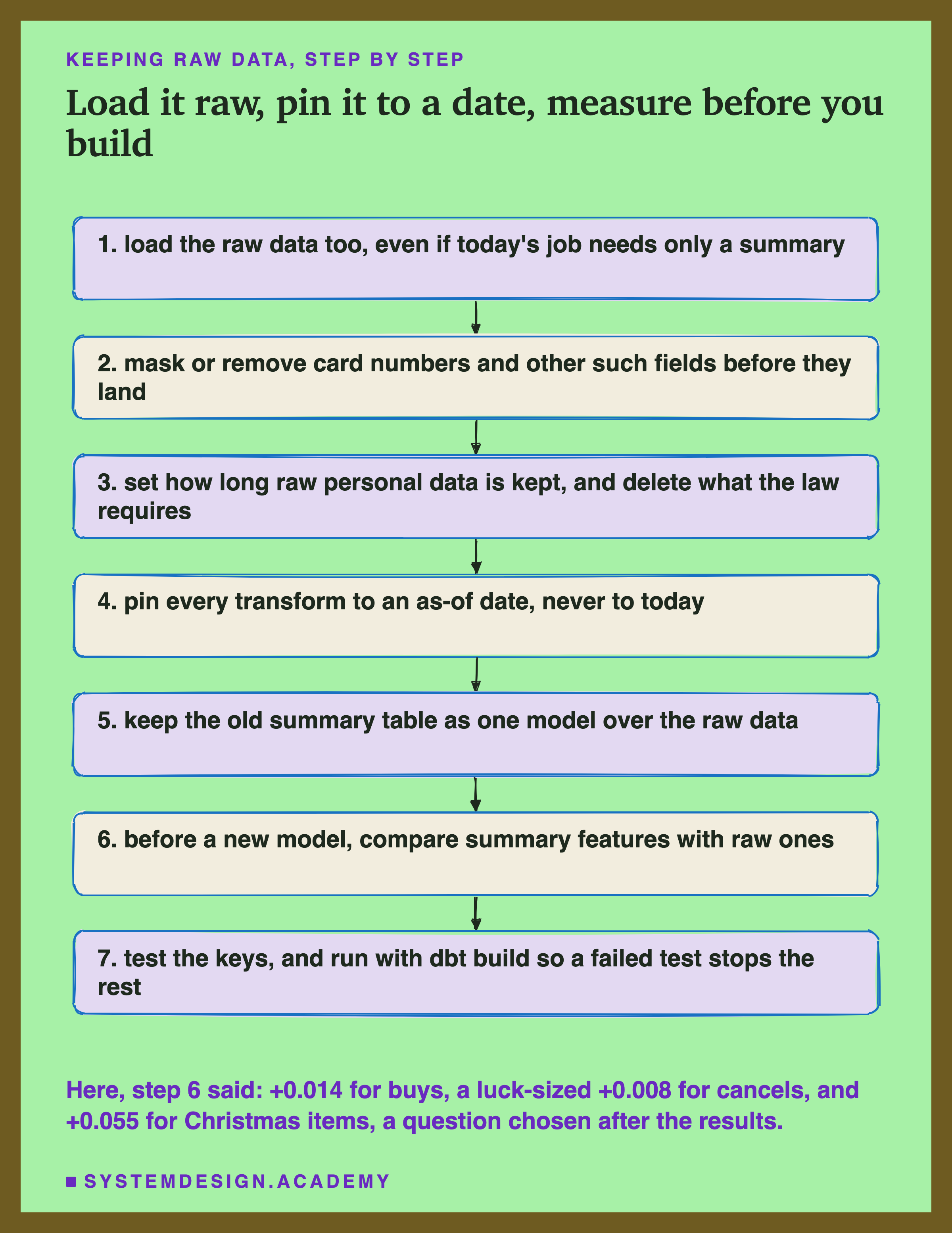
Load the raw data too. Even if today's job needs only a summary, store the rows as they arrived. Here that cost $0.00218 a month.
Mask or remove sensitive fields before they land. A card's security code must be dropped, and a card number truncated or tokenized. Masking them later is too late, because the readable values have already been stored.
Set how long raw personal data is kept. GDPR says personal data may be kept "for no longer than is necessary", and people can ask for theirs to be erased. Give the raw layer a retention period, and a way to delete one person's rows.
Pin every transform to an as-of date. A transform that reads today's date cannot rebuild last month's table. Pass the date in.
Keep the old summary table as one model over the raw data. Dashboards that read it keep working, and it can be rebuilt whenever its logic changes.
Before a new model, compare summary features with raw ones. Train once on what the summary can give, and once with raw features added. Then check the gap with a bootstrap. Here that took seconds.
Test the keys, and run with dbt build. A unique test on the invoice line and a not_null test on the customer id stop a duplicated line from inflating someone's revenue.
When to Keep Raw, When to Transform First
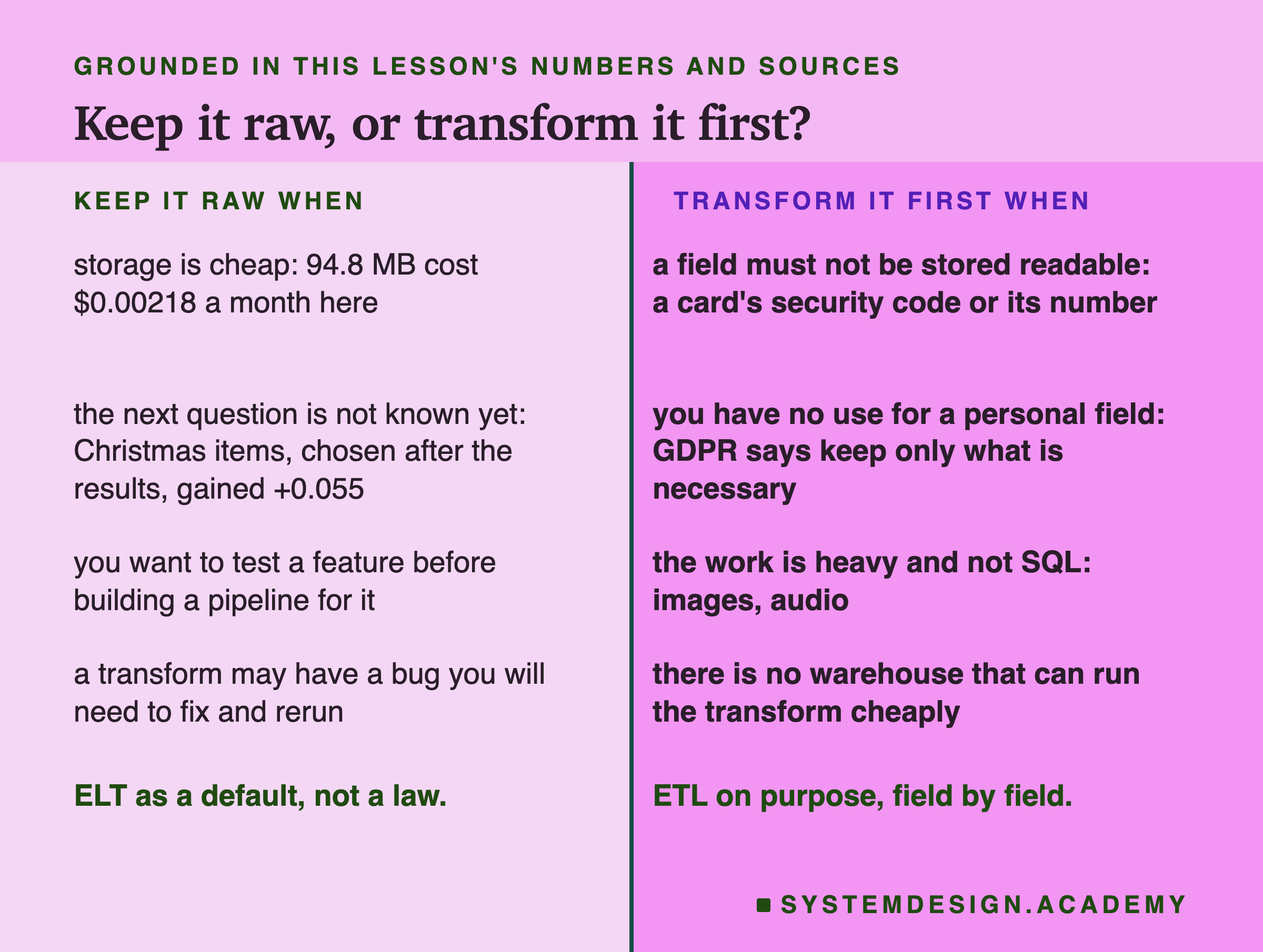
Keep it raw when storage is cheap next to what a question is worth. Here the raw lines cost $0.00218 a month, and one new question, chosen after the results, gained 0.055 AUC (0.059 with one added feature).
Keep it raw when you do not know the next question. The daily table held up on the two questions near what it recorded. It fell behind on the one about something it never recorded.
Keep it raw when you want to test a feature before building a pipeline. Every gap in this lesson took seconds to measure, because the lines were there.
Keep it raw when a transform may need fixing. A bug in a summary can be fixed and rerun only if the rows under it still exist.
Transform first when a field must not be stored readable. Drop a card's security code, truncate or tokenize its number before load, and load the rest of the row raw.
Transform first when you have no use for a personal field. GDPR says personal data must be "limited to what is necessary". If no question needs it, do not keep it.
Transform first when the work is heavy and not , or when there is no warehouse that can run the transform cheaply.
What These Numbers Can and Cannot Tell You
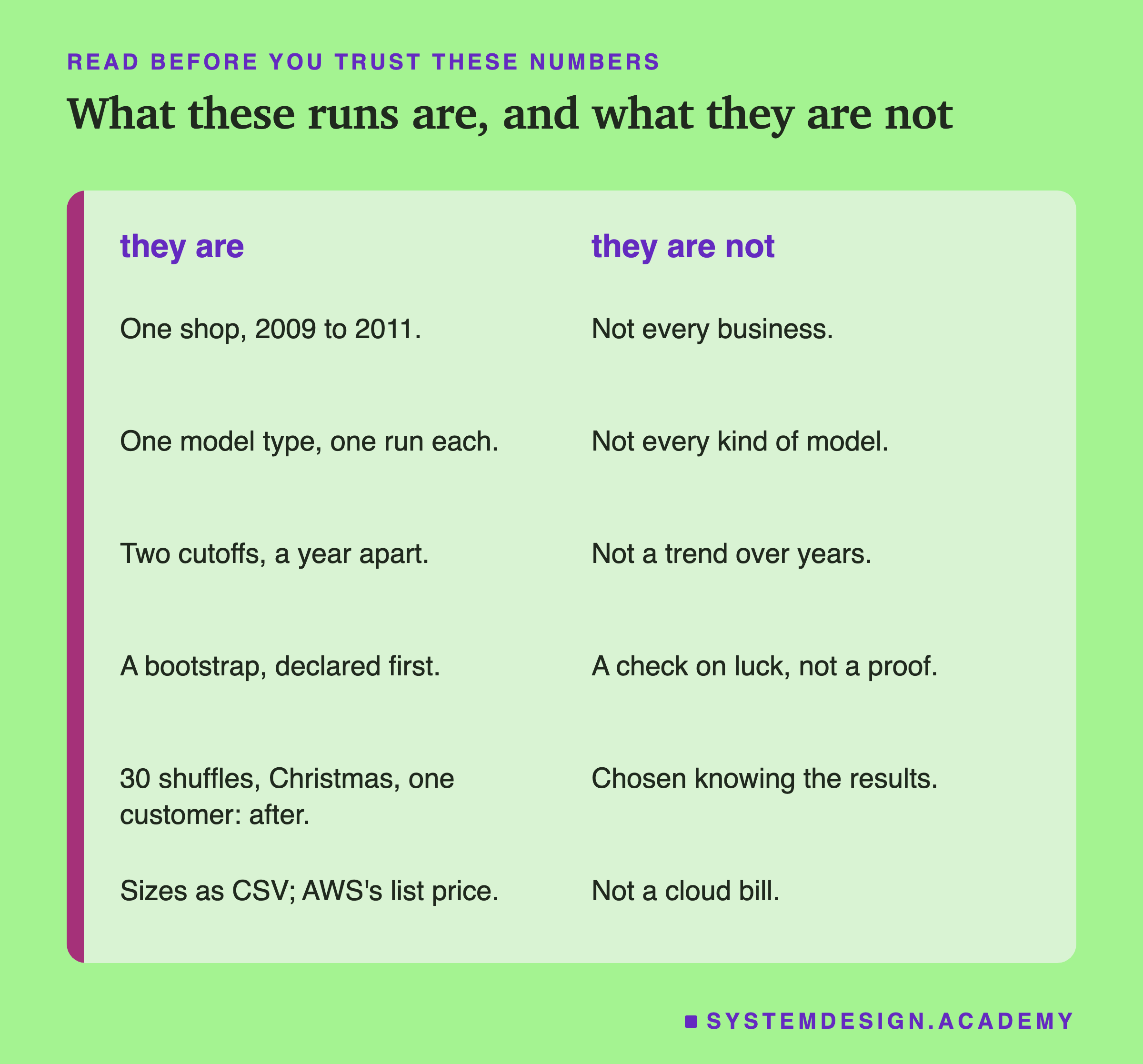
One shop, one model type, one run each. Everything here is one UK online gift shop, with many wholesale customers, from 2009 to 2011, and one kind of model. With other data, other questions and other models, the numbers would move.
Two cutoffs, a year apart. The models learned at one September and were tested at the next. That tests one step into the future, not a trend.
The bootstrap checks luck, and nothing else. It asks whether a different set of test customers from the same shop would give the same gap. For buys it held; for cancels it did not.
Some parts came after the results. The four designs, the two questions and the bootstrap were fixed before the first run. The shuffles, the Christmas question and the customer picked by a rule came later. I wrote them down before the report first ran, and the Christmas question in particular was chosen knowing the first gains were small. After a review of this lesson I also raised the shuffles from one to 30, and bootstrapped the Christmas gap for elt, not only for elt+.
Sizes, not bills. I measured the tables as CSV and priced them at AWS's list price. A real warehouse stores data compressed, and adds compute and other charges. I did not measure a cloud bill.
What to Do Next
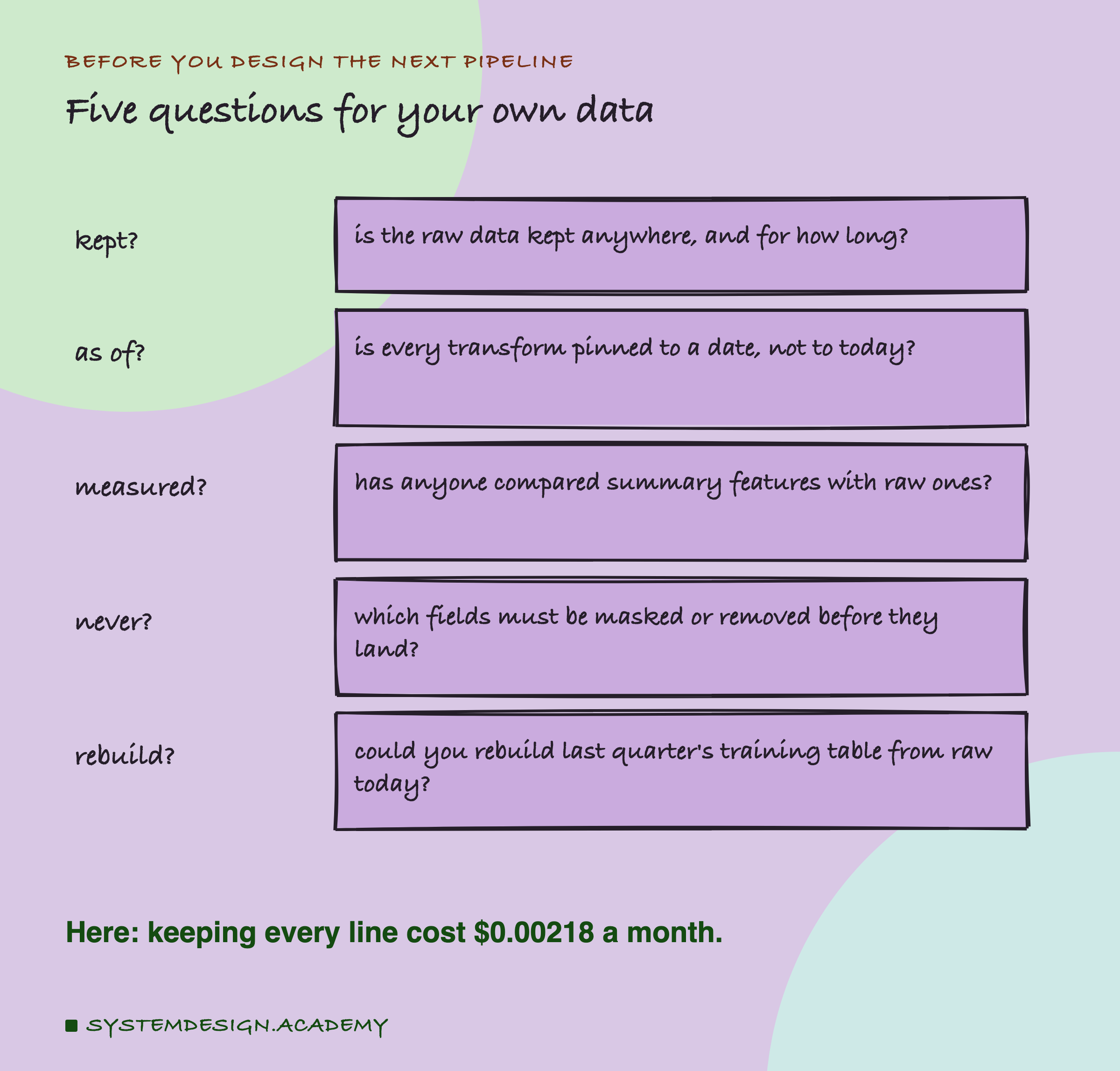
Take one pipeline your team runs and ask the five questions on the card. The first and the last are the quickest. Is the raw data kept anywhere, and could you rebuild last quarter's training table from it today? If the answer to both is no, you have the ETL design from this lesson, whatever the tools are called.
Then do the measurement. Train one model on the features your summary tables give, and one with a few features rebuilt from the raw data. Check the gap with a bootstrap. Here the gap was 0.014 on one question and luck-sized on another. On a question the summary never recorded, which I chose after the results, it was 0.055 (0.059 with one added feature). Your gaps will differ, and now you have a way to find them.
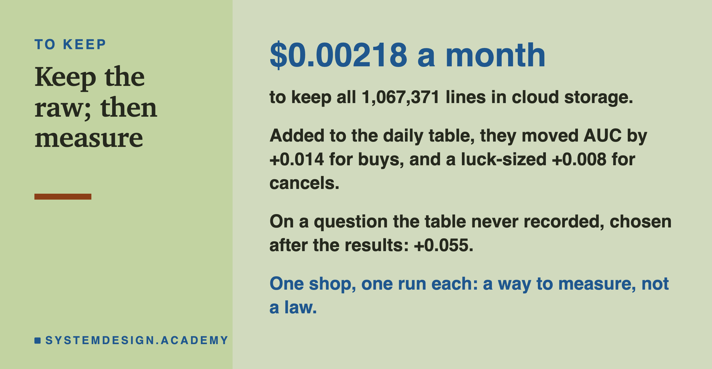
The card keeps the lesson's numbers. Keeping every line cost $0.00218 a month. On two questions near what the daily table held, the lines added 0.014 and a luck-sized 0.008. On a question the table never recorded, chosen after the results, they added 0.055, or 0.059 with one added feature.
The next lesson in this chapter is about data lakes, warehouses and lakehouses. It covers the places the raw data from this lesson can be kept, and how they differ.
Knowledge Check
Knowledge Check
4 questions - Score 80% to pass
In the lab, what did adding the 7 raw-line features to the 8 daily-table features do for the buys and cancels questions?
177 test customers cancelled something but never had a day of negative revenue in the daily table. Why?
The corrected dbt model reads its date from var('as_of') instead of current_date. Why?
Which field is the lesson's example of one that must be removed before it lands, even when the rest of the row is loaded raw?