Imagine a running club that wants to sign one new runner for the autumn season. Two hundred people come to a one-day tryout in spring. Each runs one race, and the club signs whoever is fastest. It sounds fair. But that day there was a strong wind, and it blew harder at some moments than at others. The fastest runner may simply have had the wind at her back. The more people who run, the more likely it is that the fastest time is partly wind.

There is a second problem, and it is quieter. The tryout was on a short, flat track in spring. The season is in autumn, on long hilly courses. A runner who is great on a flat sprint may be ordinary on a hill. So the club can be wrong twice: once because the winning time was partly luck, and again because the tryout tested a different kind of race from the one that matters.

This lesson does the same thing to a program that learns from examples. I tried 200 versions of one program and kept the one that looked best. Then I checked it on later months that had played no part in the choice. The winner looked better than a random pick on the months I chose with, and worse on the months that came after. The rest of the lesson measures how much of that was the wind, and how much was the wrong track.

Two words first. Accuracy is the share of guesses that were right, and a point is one hundredth of accuracy, so going from 0.70 to 0.73 is a gain of 3 points. This chapter follows a model through its life. Start with the dumbest model showed that on this data a baseline, a simple rule that a model must beat, beat every trained model on the future. The rule, called persistence, has no learning at all: it says whatever the last half-hour was. Same code, different model trained one model 20 times with the same code and got 20 different models, because a default setting set aside a random tenth of the training rows. The seed alone moved accuracy by 7.3 points.

That lesson ended with a question. If a team tries many versions and keeps the best, how much of the winner's lead is real? That is what this lesson measures.

The pipelines lesson, training pipelines and orchestration, has a slide called "Experiment Tracking: Every Run Logs What It Did". It explains, in words, how a tracking store records every run so that a team can sort the runs by a score and find the best one. I will not repeat it. This lesson measures what happens next: when you sort 200 runs by a score and pick the top one, what that top score is worth.

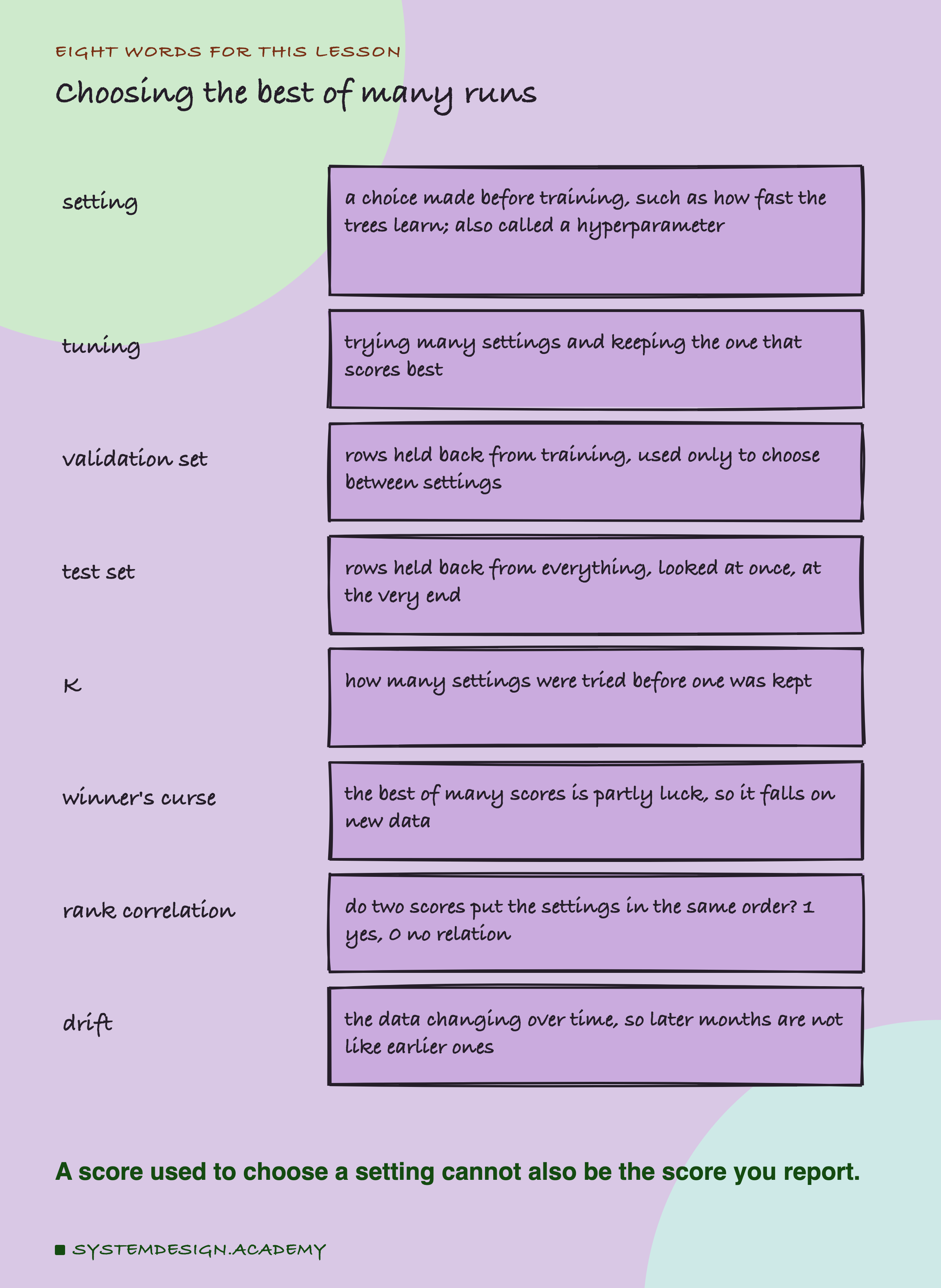
A model is a program that learned from examples. Before it learns, someone has to make some choices that the learning itself does not make: how big each step of learning is, how complicated the model may get, how long it trains. Each of these is a setting. In machine learning they are usually called hyperparameters, to tell them apart from the numbers the model learns by itself. Tuning means trying many settings and keeping the one that scores best.

To choose fairly, you need rows the model did not learn from. The validation set is a block of rows held back from training and used only to compare settings. The test set is a second block, held back from everything, including the choosing, and looked at once at the end. K is how many settings were tried before one was kept.

The winner's curse is the name for a simple fact: when you pick the best of many noisy scores, the best one is usually lucky, so it scores lower when you measure it again. A rank correlation asks whether two scores put things in the same order: 1 means the same order, 0 means no relation at all, and a negative number means a reversed order. The kind used here is Spearman's rank correlation, which compares the two orders, not the raw scores. Drift means the data changing over time.

One word needs care, because lesson 2 used it differently. There, the validation slice was a random tenth of the training rows that early stopping set aside inside one training run. Here, the validation set is a separate block of later months, outside training, used to compare whole settings. They share a name and not much else.

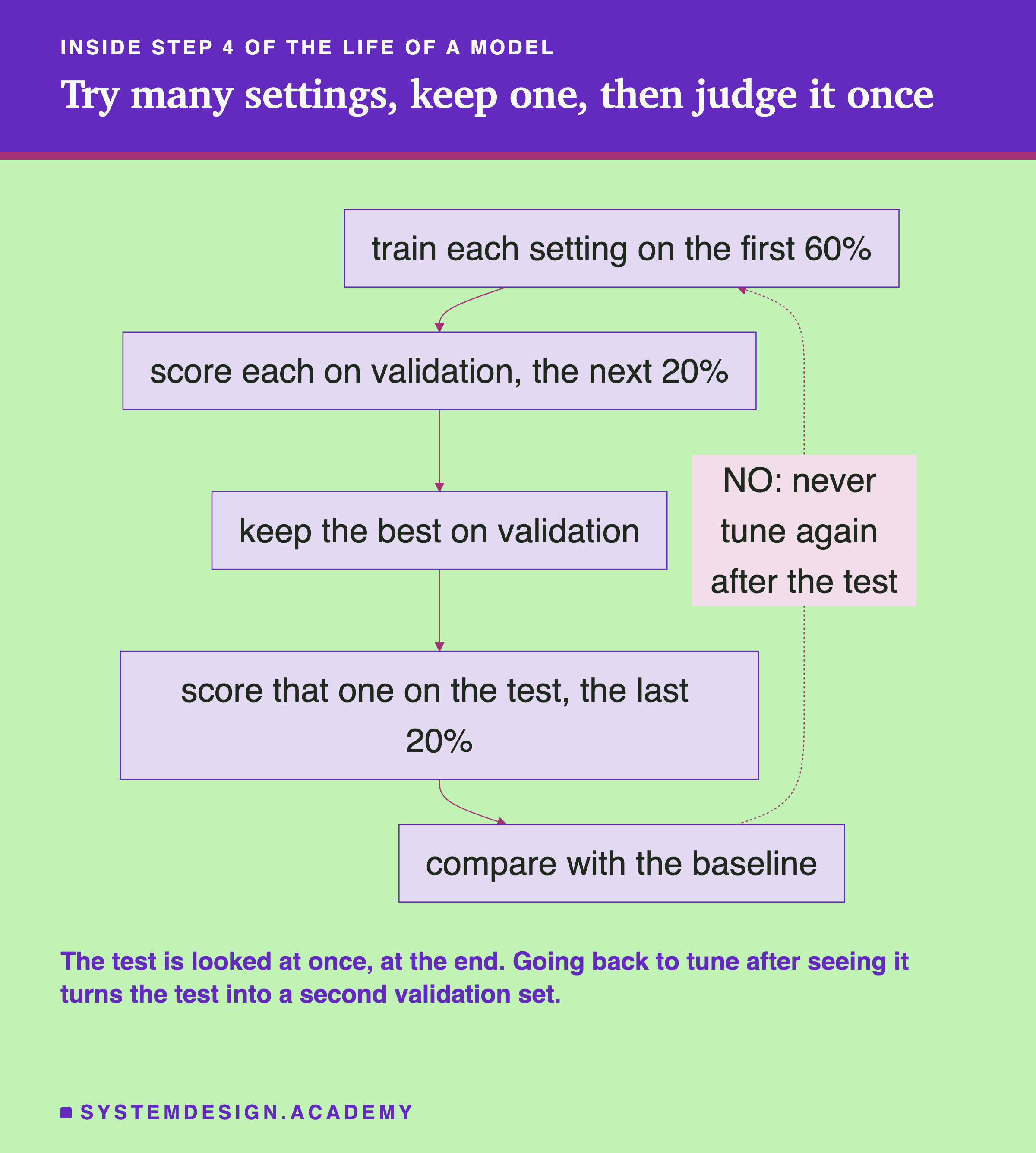
Lesson 1 cut the data into two parts, training and test. Tuning needs three, because it adds a job: choosing. Each pile gets exactly one job, and the jobs must not mix.

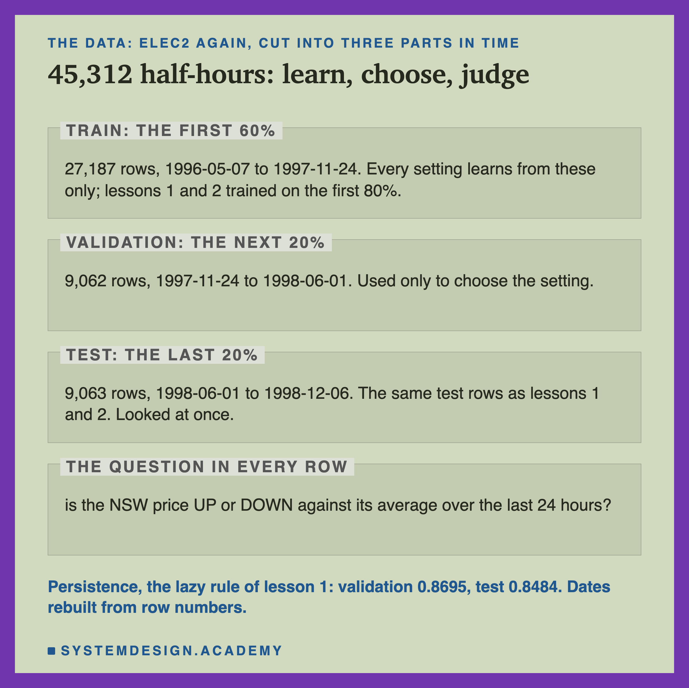
Training rows are what each setting learns from. Validation rows are for choosing: every setting is scored on them, and the best is kept. Test rows are for judging the one you kept. The data is Elec2 again, 45,312 half-hours of the New South Wales electricity market in time order, and each row asks whether the price is UP or DOWN against its own average over the last 24 hours. Because the rows are in time order, the three parts are cut in time: training is the oldest 60%, validation the next 20%, and test the newest 20%, the same test rows as the two lessons before.

Keep one thing in mind all through the lesson. Every one of the 200 settings learns from the first 60% only, so its scores sit below those in lessons 1 and 2, which trained on the first 80%. The default trees with early stopping off, the same model as lesson 2's, scored 0.7520 on test when trained on 80% there, and 0.7077 when trained on 60% here.

Why must the test be touched only once? Because the moment you use a score to make a choice, that score stops being a fair estimate. If I look at the test, go back, change a setting, and look again, I am choosing on the test, and the test has become a second validation set. Its number then carries the same optimism as the validation number, and I have no clean number left to report.

Why not just choose on the test and skip validation? For the same reason. The score you choose on is the score that flatters you. You need one set to choose on and a different set to find out what the choice is worth.

I wrote the lab's design at the top of its file, select_lab.py, before it ran. The dated record is in the chapter plan (2026-09-29, "SELECT LAB (batch 3) designed before running").

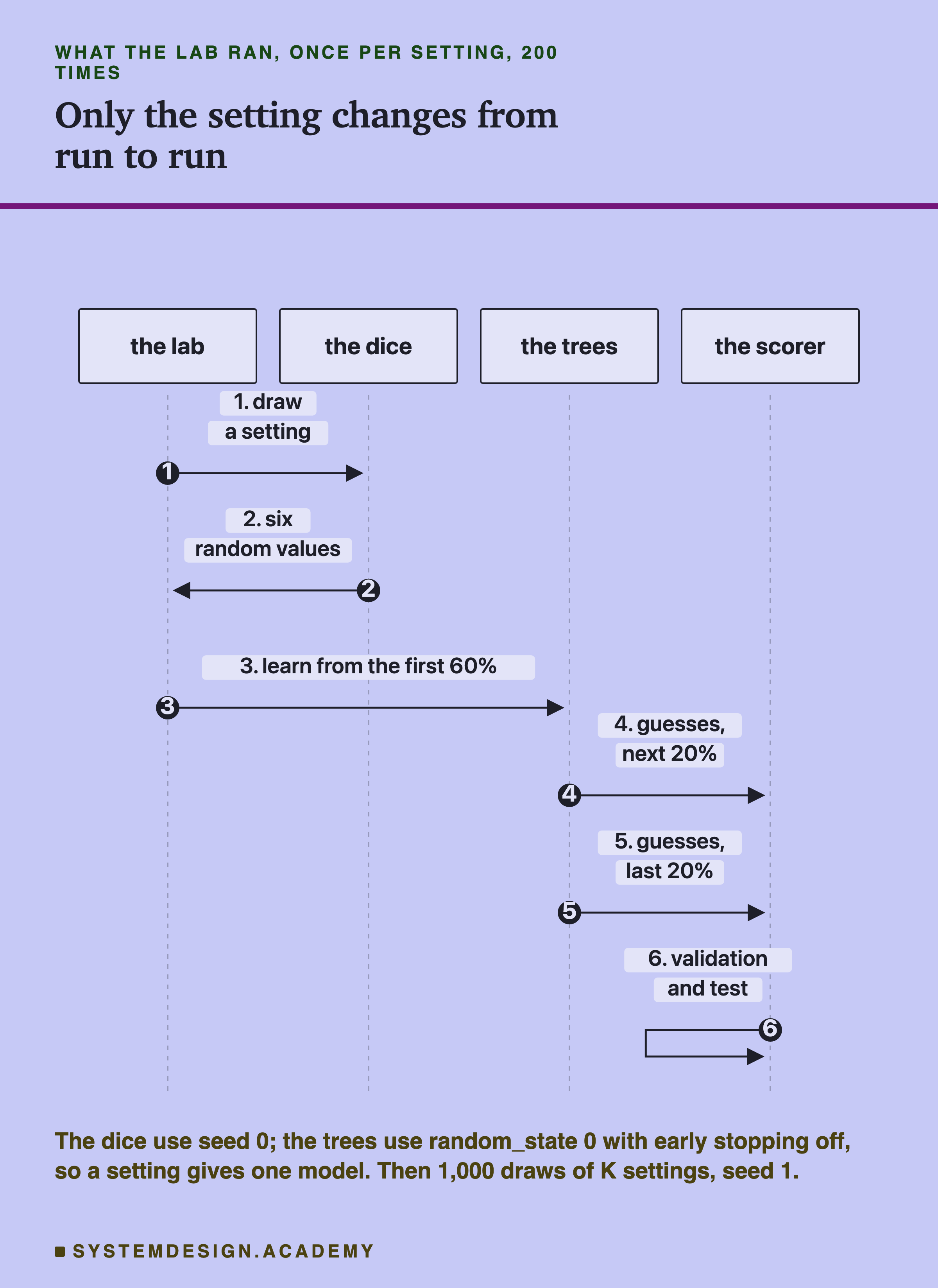
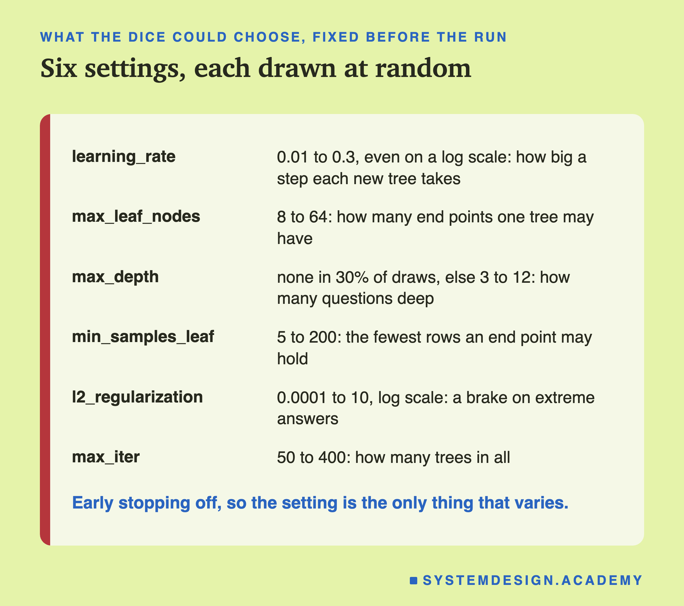
The model is scikit-learn's HistGradientBoostingClassifier, the boosted trees from lessons 1 and 2: many small trees of yes-or-no questions, built one after another, each correcting the mistakes of the ones before. The 200 settings were drawn at random from fixed ranges, written down before the run. Early stopping, a rule that stops adding trees once a held-out slice of the training rows stops improving, was switched off. The trees used random_state=0, scikit-learn's name for the seed of their random choices. Two of the ranges are log scale, which means each tenfold step is equally likely: a learning rate between 0.01 and 0.03 is as likely as one between 0.1 and 0.3. Lesson 2 found that with early stopping off, its trees came out the same whatever the seed, and here the seed is fixed anyway. So each setting gives exactly one model, and the only thing that varies from run to run is the setting.

Here is the headline, from the lab's stored file, results/select.json.

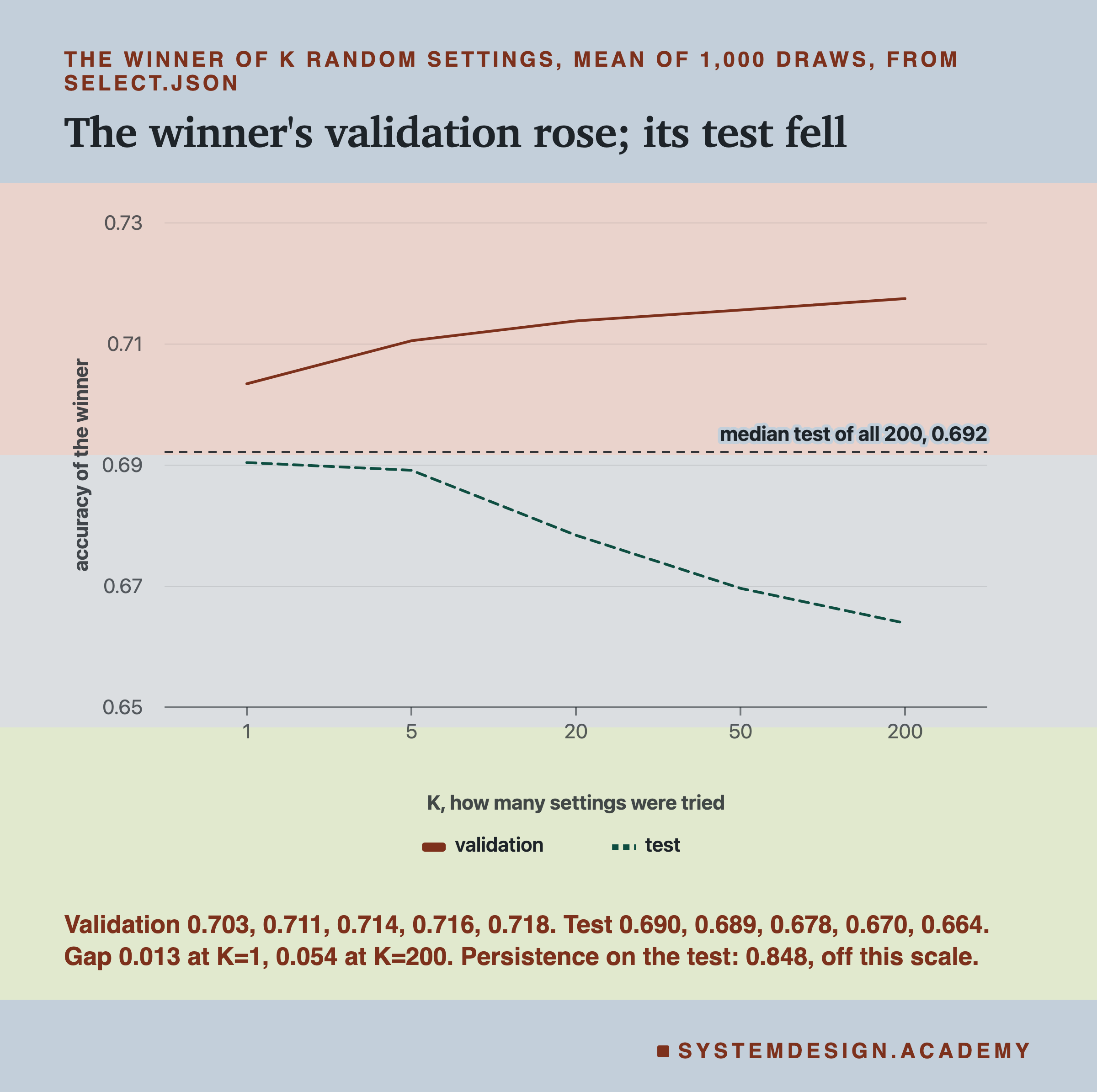
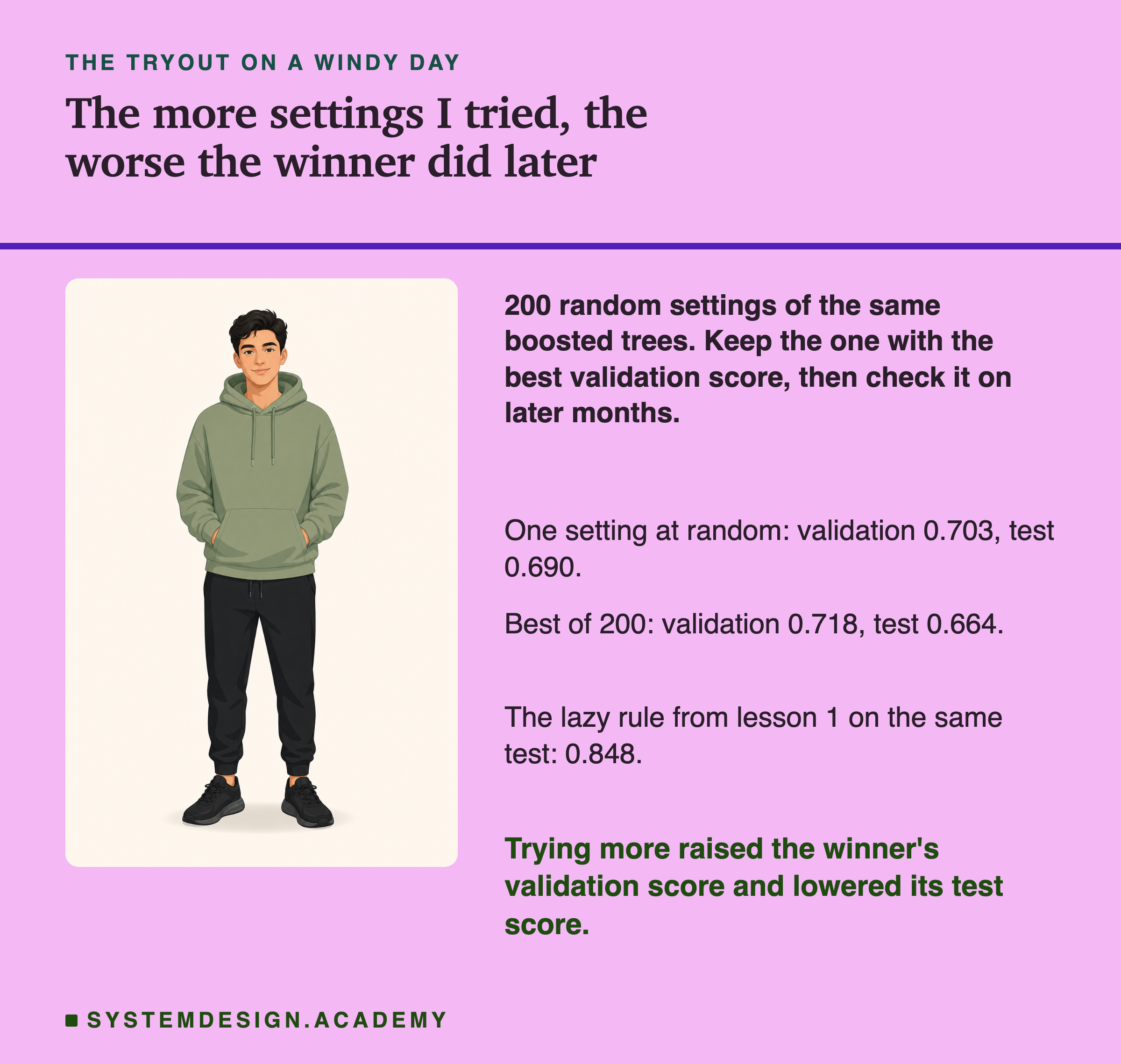
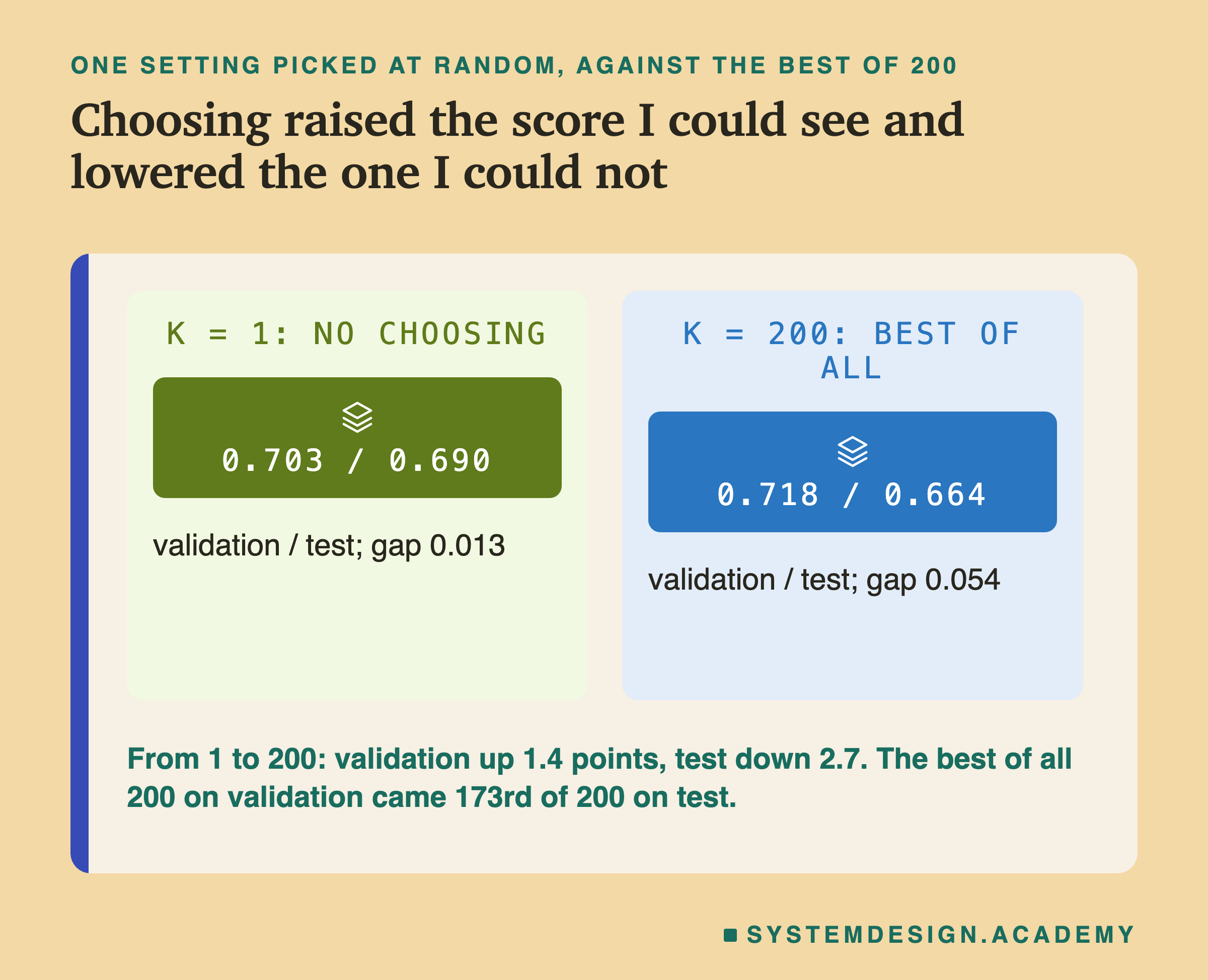
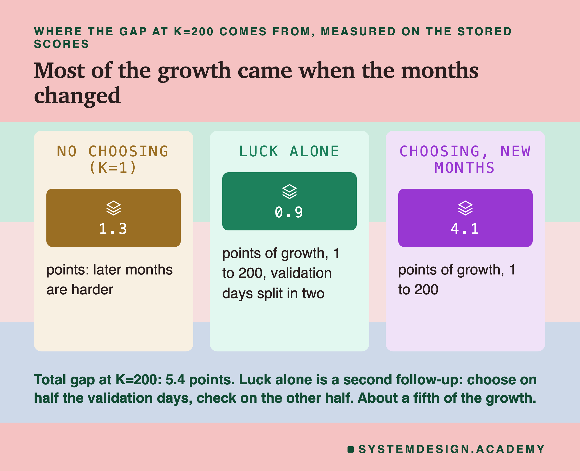
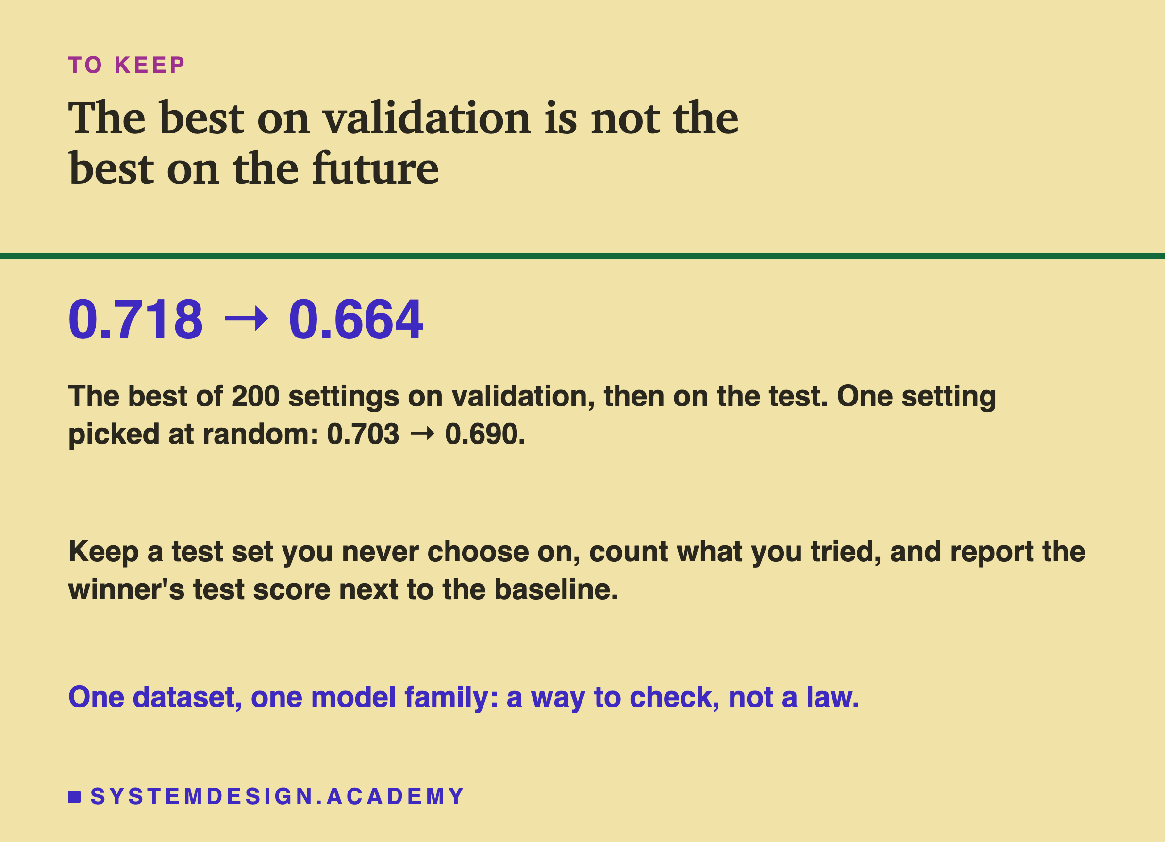
With K = 1, no choosing at all, the kept setting scored 0.7034 on validation and 0.6904 on test, a gap of 0.0130. With K = 200, the best of all of them, it scored 0.7175 on validation and 0.6639 on test, a gap of 0.0536. In between, the pattern is steady: the more settings I tried, the higher the winner's validation score and the lower its test score. From K = 1 to K = 200, validation rose by 1.4 points and test fell by 2.7 points.

Look at where the test line ends. The median test score of all 200 settings, the middle one if you line them up, was 0.6922. The winner of 200 scored 0.6639 on test: it came 173rd of the 200. Choosing did not just fail to help here. It picked a setting that was worse on the future than a setting picked with no care at all. With K = 20 the winner fell below that median in 71% of the draws, and with K = 50 in 92%.

And the lazy rule from lesson 1, persistence, which says whatever the last half-hour was, scored 0.8484 on the same test rows. The best test score of any of the 200 settings was 0.7502. No setting came close.

Choosing on validation can only work if a setting that is good on validation tends to be good on test. So I put each setting's two scores side by side.

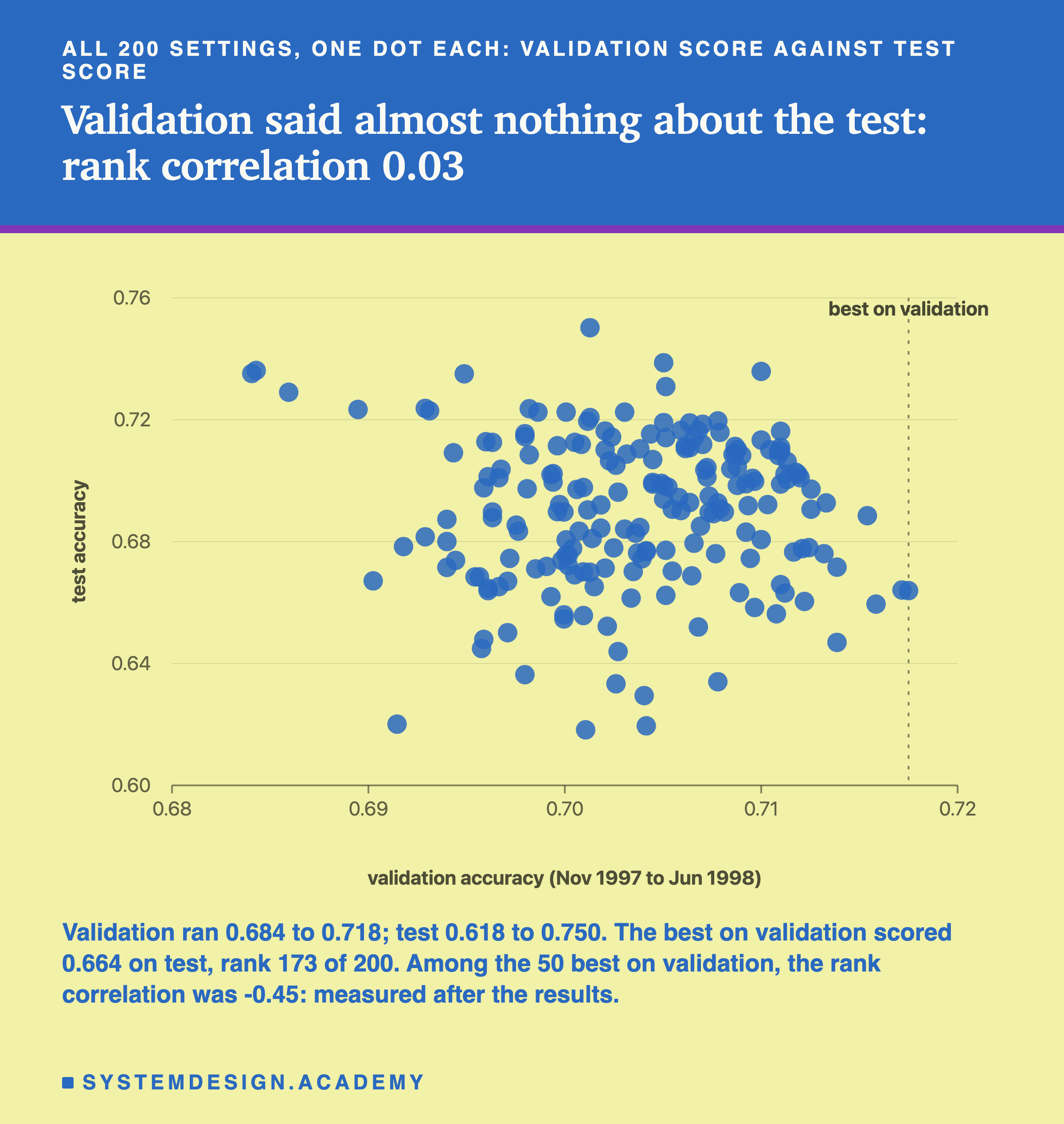
The rank correlation between validation and test, over all 200, was 0.03: almost no relation. Knowing a setting's validation score told me close to nothing about its test score. Worse, among the 50 settings that did best on validation, the rank correlation was -0.45, a clear reversed order: in this top group, the better a setting looked on validation, the worse it tended to do on test. That second number I measured after I saw the results.

Two more things stand out in the stored scores. The settings were close on validation, 0.6841 to 0.7175, a range of 3.3 points. On test they were spread four times as wide, 0.6182 to 0.7502. So the validation months could barely tell the settings apart, while the test months separated them strongly, and in a different order.

The setting that was best on test, number 143, scored 0.7502 there. Its validation score was 0.7013, below the validation median of 0.7039. Nobody choosing on validation would ever have kept it.

Here is the general idea, before I split this lab's result into its parts. Think of every score as two pieces added together: how good the setting really is, and luck. On any finite set of rows, some settings happen to get lucky rows and some get unlucky ones.

When you pick the highest of many scores, you are more likely to pick one whose luck was good. On new rows the luck is new, so the winner's score usually falls back. The more settings you try, the more extreme the luckiest one, and the bigger the fall. That is the winner's curse, and it happens even when nothing about the world changes.

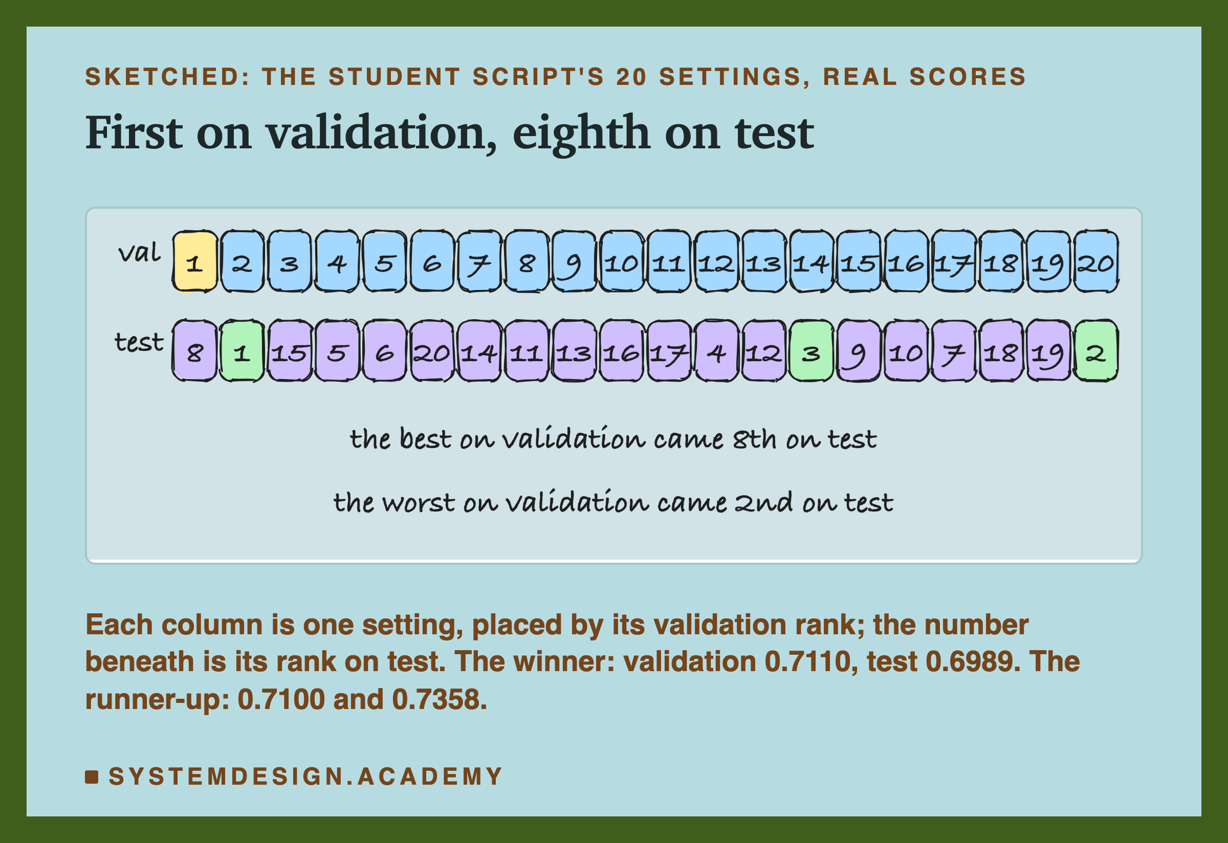
The sketch is the student script's 20 settings, the lab's first 20, with real scores. The winner on validation came 8th of 20 on test. The runner-up, just 0.001 behind it on validation, was the best of the 20 on test. And the setting that was worst on validation came 2nd on test. With 20 settings this is one draw, not a rule. The lab's 1,000 draws of 20 are the rule: on average, the winner of 20 scored 0.6784 on test, below the 0.6922 median.

But notice something the plain curse does not explain. When validation and test measure the same thing, luck on its own should make the winner's test score fall back toward the average, not past it. A lucky winner is still, on average, at least as good as a random pick. Here the winner of 200 fell well below the median. Something more than luck is at work, and the next slides find it.

The validation rows are November 1997 to the first morning of June 1998. The test rows are June to December 1998. They are different months, and on this data that matters. I compared the two parts after I saw the results.

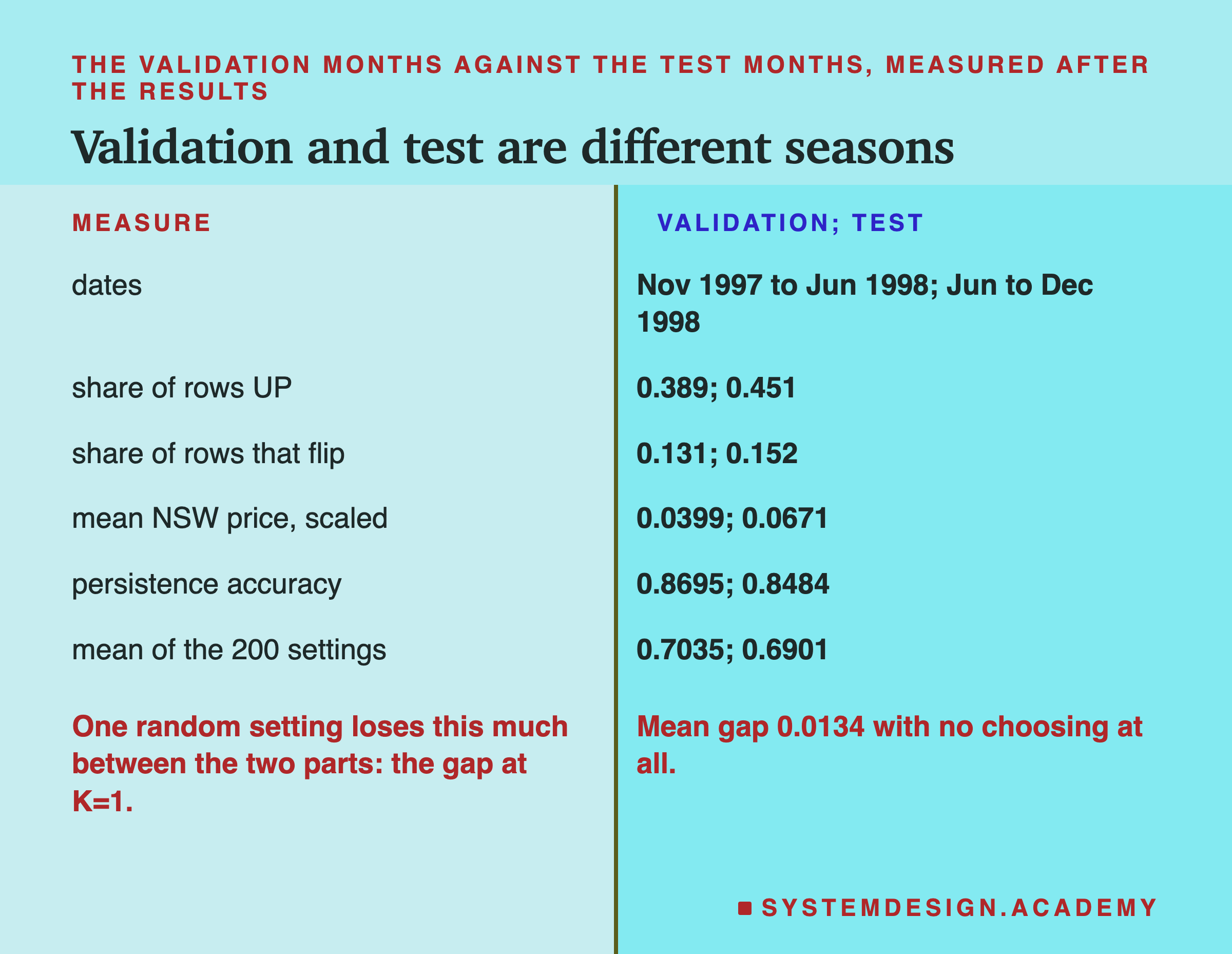
The two parts differ in plain ways. In the validation months the price was UP on 38.9% of rows; in the test months, 45.1%. The average scaled price was 0.0399 in validation and 0.0671 in test, and 0.0608 over the training rows here. Lesson 1 gave 0.0556 for its training rows because it averaged the first 80%, which includes the calm, cheap validation months. The label changed from one half-hour to the next, a flip, on 13.1% of validation rows and 15.2% of test rows. Even the lazy rule noticed: persistence scored 0.8695 on validation and 0.8484 on test.

So some of the gap is there before any choosing. The average setting scored 0.7035 on validation and 0.6901 on test, a gap of 0.0134, almost exactly the 0.0130 gap at K = 1. That part is not the winner's curse at all. It is drift: the test months were simply harder for these trees than the validation months.

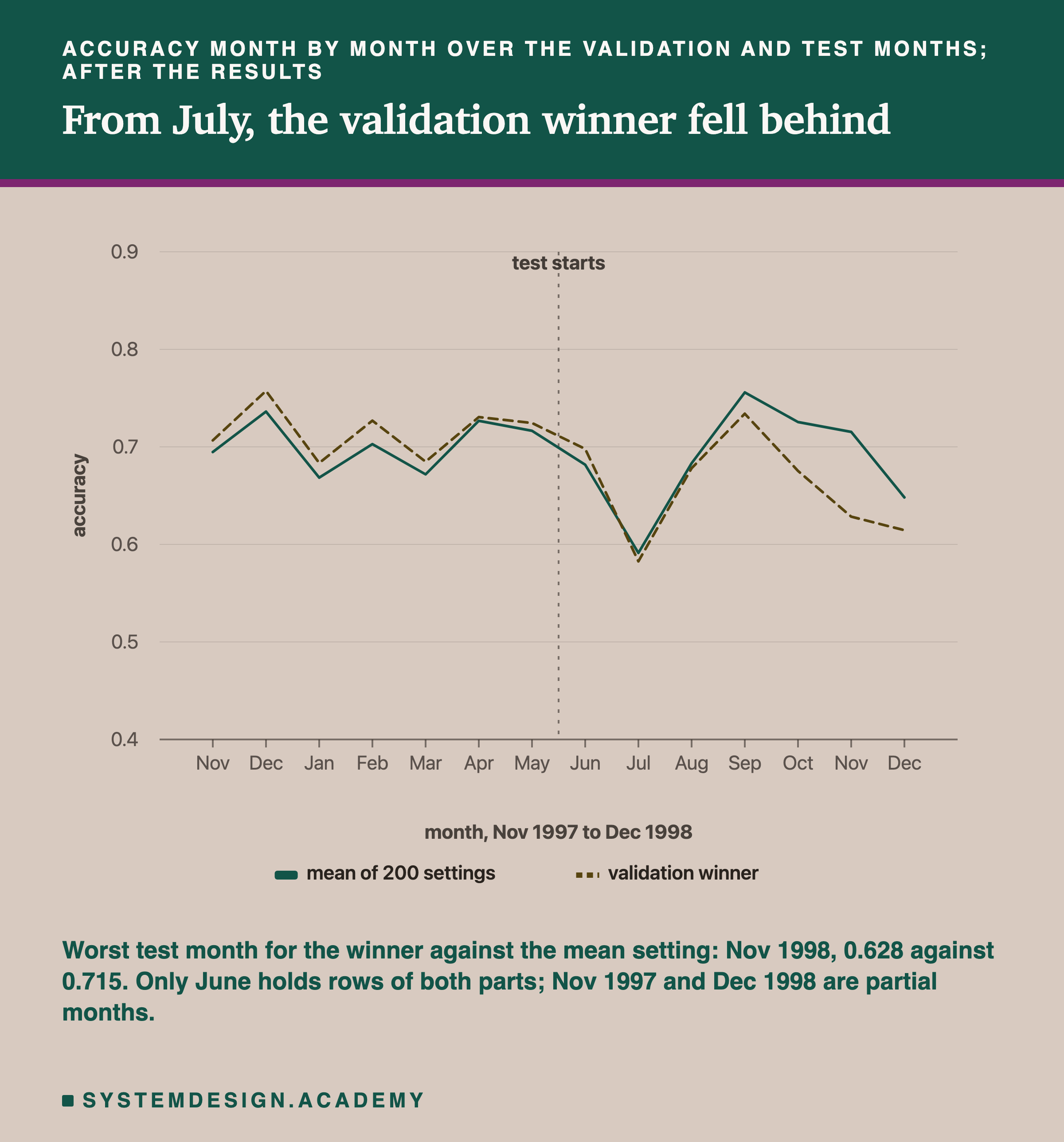
The month-by-month numbers show more. In every validation month, the validation winner scored at or above the average setting, as you would expect from the setting chosen on those months. In June, the first test month, it was still ahead, 0.698 against 0.682. From July it fell behind, most of all in October, 0.675 against 0.725 for the average setting, and November, 0.628 against 0.715. July was hard for every setting (0.591 on average), the same July that lesson 1's trees broke down in.

Two causes are mixed in the main result: selection luck, and the change of months between validation and test. The stored scores alone could not separate them, so I added a follow-up to the lab. I designed it after I saw the main results, and I wrote its design into the lab file's followup mode before it ran. Its results are in results/select_followup.json.

The idea is a control: the same experiment with one thing changed. I trained the same 200 settings again on the same training rows (every validation and test score came back identical to the stored ones, to twelve decimal places). Then I made a control split by days: I pooled the validation and test months together and assigned each whole day, at random, to one side or the other: half the days became a control validation set, the other half a control test set. Now both sets come from the same months. If the main gap were selection luck, it should appear here too. I did this with 20 different random splits.

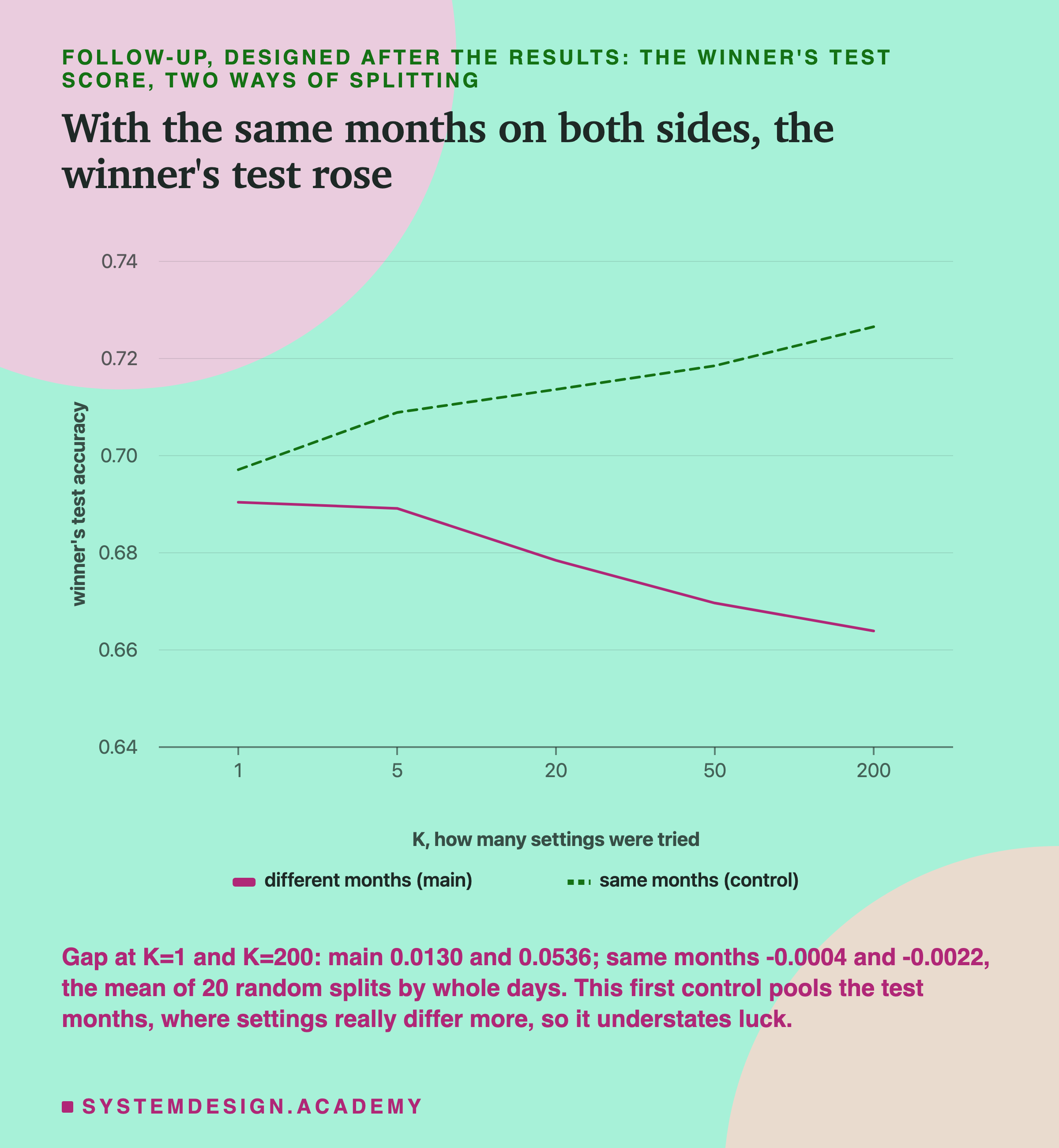
With the same months on both sides, the rank correlation between control validation and control test was 0.89 on average (0.71 to 0.96 across the 20 splits), against 0.03 in the main split. Choosing worked: the winner's control test score rose with K, from 0.6971 at K = 1 to 0.7265 at K = 200, almost exactly as fast as its control validation score rose. The gap stayed near zero at every K: -0.0004 at K = 1 and -0.0022 at K = 200, on average over the 20 splits.

If the two parts reward different settings, it should show in which settings did well on each. So I measured, after the results, the rank correlation of each of the six settings with the validation score and with the test score, over all 200.

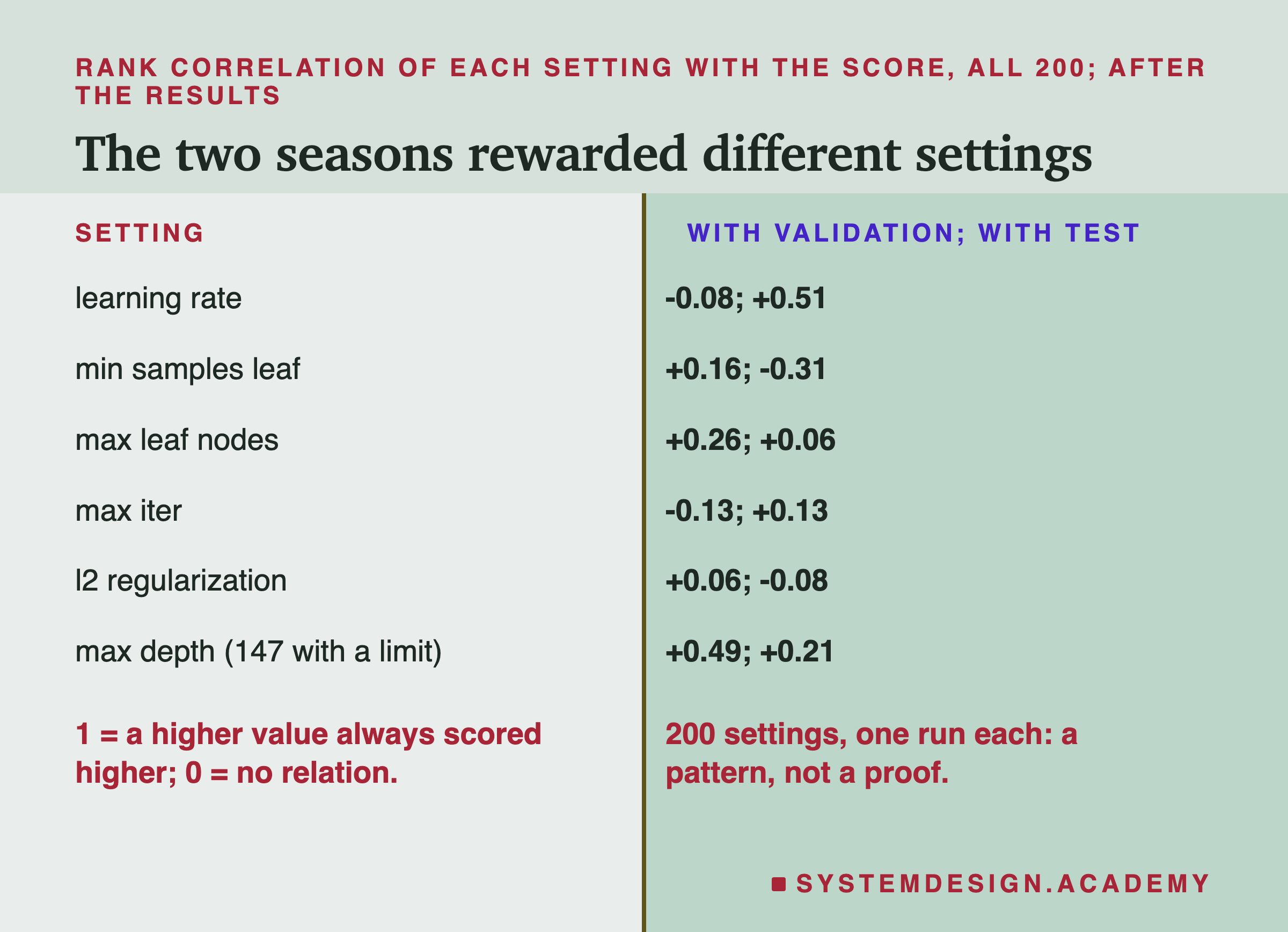
The clearest line is the learning rate, how big a step each new tree takes. On validation it made almost no difference (-0.08). On test, faster learners did clearly better (+0.51). min_samples_leaf, the fewest rows an end point of a tree may hold, went the other way: slightly good on validation (+0.16), bad on test (-0.31). The top five settings on validation all had small learning rates (0.012 to 0.059) and large leaves (123 to 197 rows). That is a description of these 200 settings, not a proof.

Why would the test months reward faster, finer trees? One possible reason, and it is a guess I have not tested: the test months had higher prices and more flips than the validation months, and the training period, so a model that adapts more sharply to its inputs may cope better with prices it rarely saw. The validation months had low, calm prices, where a slow, smooth model loses little. I measured the price levels and flip rates; I did not measure the reason.

Lesson 2 found that the seed alone moved one setting's accuracy by 7.3 points. That is a lot of noise. How much noise is there in one validation score here?

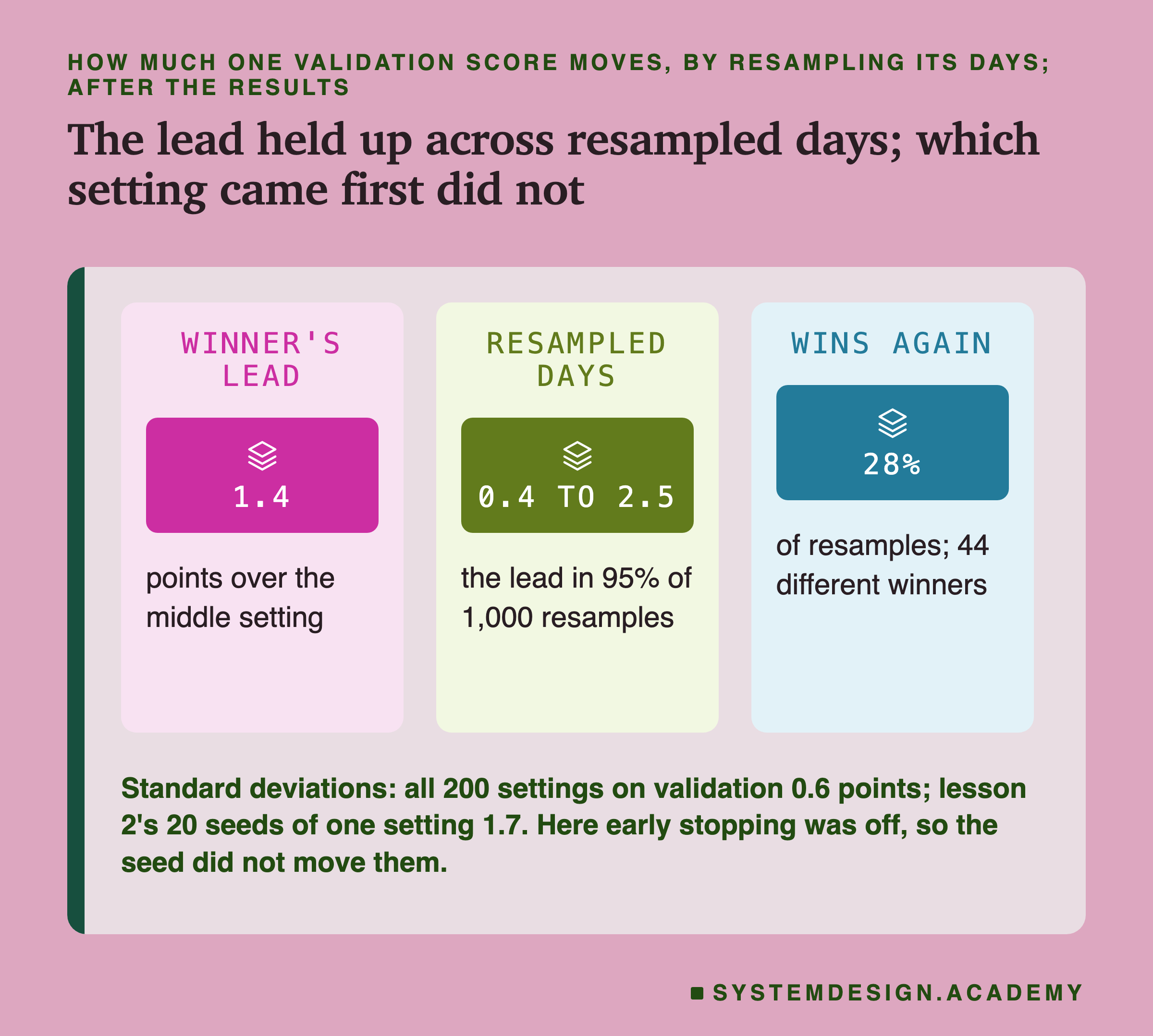
I measured it with a bootstrap, after the results: make 1,000 new samples of the 190 validation days, each drawn at random with repeats allowed, and score the settings on each sample. Whole days are drawn, not single half-hours, because neighbouring half-hours are alike. A standard deviation measures how far values usually sit from their average. Across the samples, the winner's validation score had a standard deviation of 0.0140: most samples put it within about 1.4 points of its real value.

Its lead over the middle setting was 1.37 points, and that lead held up across resampled days: in 95% of the samples it stayed between +0.43 and +2.46. But which setting came first did not hold up. A second follow-up picked the best of all 200 again on each of 1,000 resampled sets of validation days: the original winner won again in only 28% of them, and 44 different settings won at least once. So the lead of one chosen pair was steady, while the choice itself was fragile, and neither said anything about the test months.

Now the link to lesson 2, comparing like with like. Here I switched early stopping off, so each setting gave one model and the seed changed nothing. The 200 settings' validation scores had a standard deviation of 0.62 points. In lesson 2, with early stopping at its default, the 20 seeds of one setting had a standard deviation of 1.72 points. If I had left the default on here, each setting's score would have carried seed noise almost three times as large as the usual difference between settings, and picking the top score would mostly have picked the luckiest seed. That is a reasoned expectation from two measured numbers; this lab did not run it.

The follow-up also tried two other ways of choosing, both designed after the main results.

Two windows. Each setting was also trained on the first 40% of rows and scored on the next 20% (May to November 1997), an earlier window. Its selection score was the average of that earlier score and its normal validation score. This is a small version of a forward scheme: judge each setting on more than one later window, each time training only on what came before, the way the model will really be used.

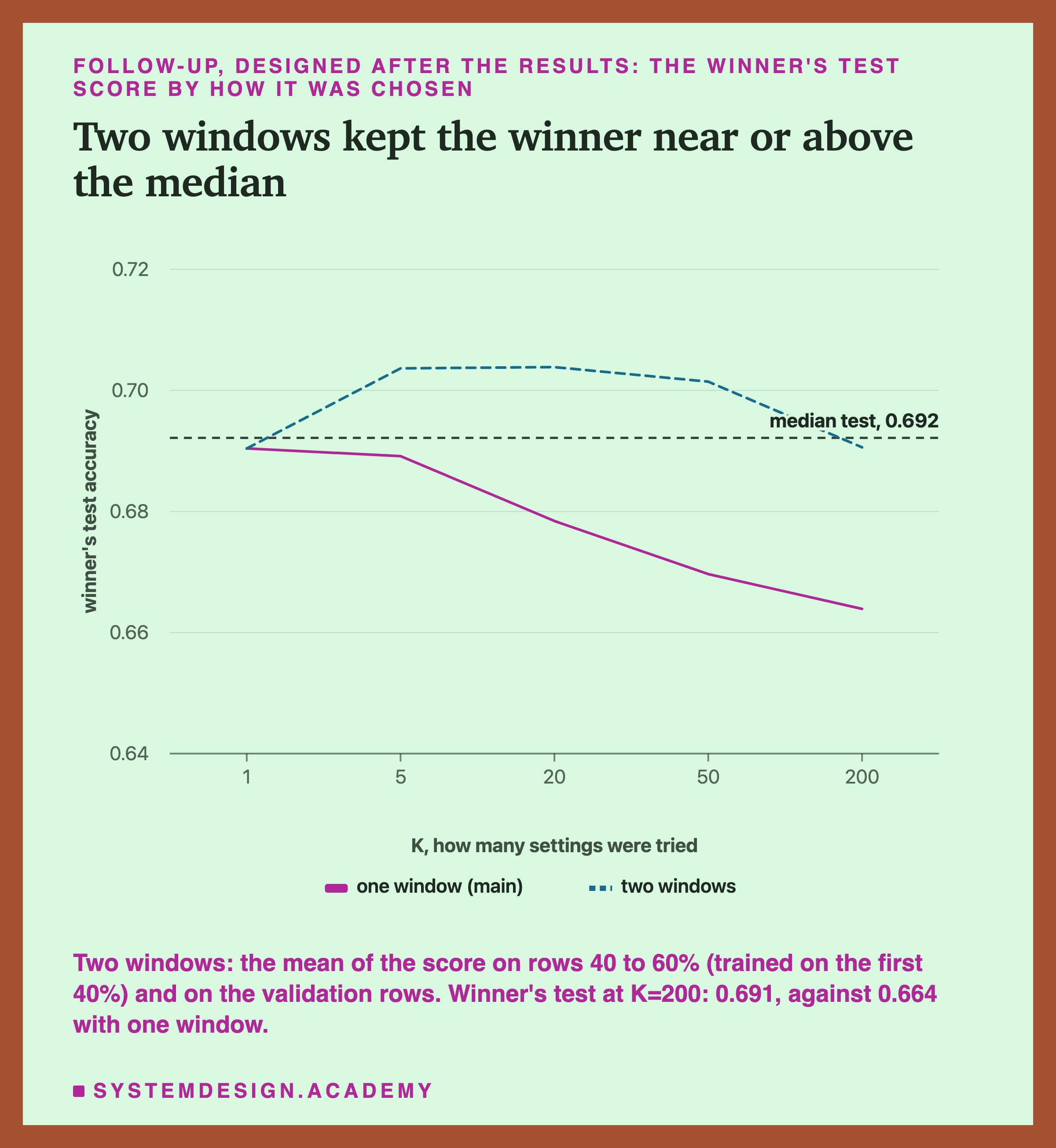
It helped, partly. With two windows the winner's test score was 0.7037 at K = 5 and 0.7038 at K = 20, above the 0.6922 median, against 0.6892 and 0.6784 with one window. At K = 200 it fell back to 0.6906, about the median. The earlier window happened to agree with the test months better than the validation months did: its rank correlation with test was 0.62, and with validation -0.11. That is luck of this calendar as much as a rule; with other data the earlier window could be the one that misleads.

The reverse. Choosing on the test months and checking on the validation months, from the stored scores, gave the mirror image: the winner's validation score fell from 0.7034 at K = 1 to 0.6980 at K = 20, below the validation median of 0.7039. So the mismatch runs both ways. It is not that the test months are special; it is that these two seasons reward different settings.

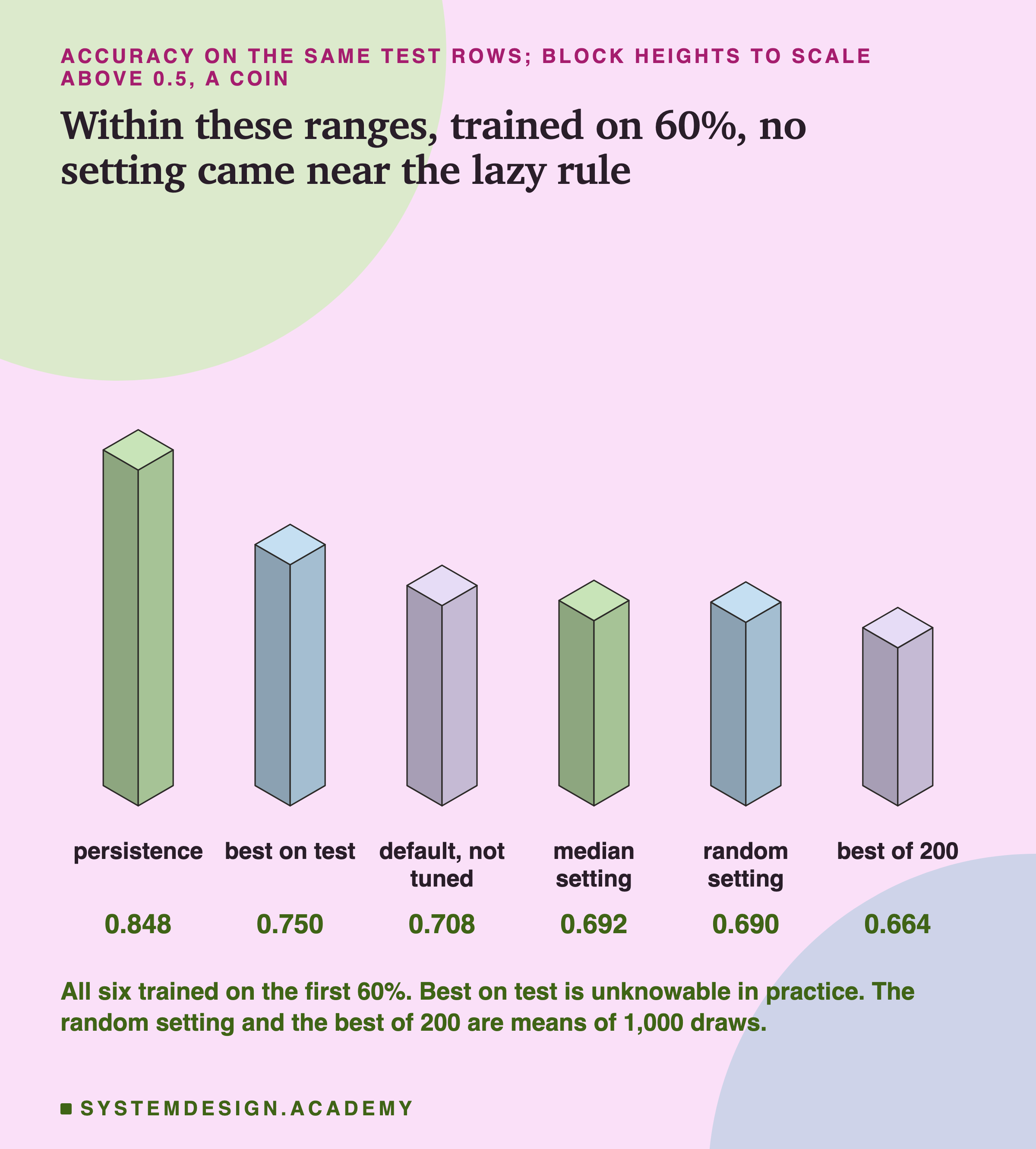
One more comparison matters most. The best of the 200 settings on the test itself is a number you could only find by choosing on the test, which breaks the rule of this lesson. Even that setting stayed far below persistence. Within these ranges, trained on 60%, tuning could not have closed the gap. And the default setting, not tuned at all and trained on the same 60%, scored 0.7077 on test: above a random setting and above the average winner at every K.

Here is what the lab points to, in the order a team meets it.

Hold out a final test set, and touch it once. In this lab that is what made the damage visible at all. The validation score of the best of 200 was 0.7175, the best number in the whole lab. Only the untouched test showed 0.6639.

Report the winner's test score, not its validation score. The validation score of a winner is the score you chose with, so it is always too high: it was picked because it was high. Here the report would say 0.664, not 0.718.

Keep count of how many settings you tried. K belongs next to the score. A winner of 5 and a winner of 200 do not mean the same thing: here their validation scores differed by only 0.7 points, and their test scores by 2.5. An experiment tracker records every run, as the pipelines lesson explains; the count is simply the number of rows in it.

Prefer a smaller or simpler search. On this data, when you choose on one window of changing data, a winner of 5 did about as well on test as a random pick (0.6892 against 0.6904), and every larger search did worse. A default setting that you did not tune has no winner's curse at all: here it scored 0.7077 on test, above the average winner at every K.

Choose on more than one window. For data in time order, a forward scheme scores each setting on several later windows, each trained only on what came before. In general, nested validation puts the whole search inside an outer loop: an inner split chooses, an outer split judges the choice, and the outer score includes the cost of choosing. Here two windows kept the winner near or above the median; I did not test more windows or a full nested scheme.

Why a forward or nested scheme costs more. Each extra window means training every setting again on a different stretch of the past, so two windows cost twice the training of one, and a full nested scheme costs the whole search once for every outer split. For trees that train in a few seconds, like these, that is nothing. For a model that trains for a day, it is a real budget, and a smaller search with more windows is often a better use of it than a larger search with one. The extra training buys two things: a choice made on more than one season, and a final score that already counts the effect of choosing, instead of one that hides it.

Compare the winner with the baseline, on the test. Here persistence scored 0.8484 and the tuned winner 0.6639. A search can only choose between the settings you give it; it cannot tell you that a rule with no learning is better.

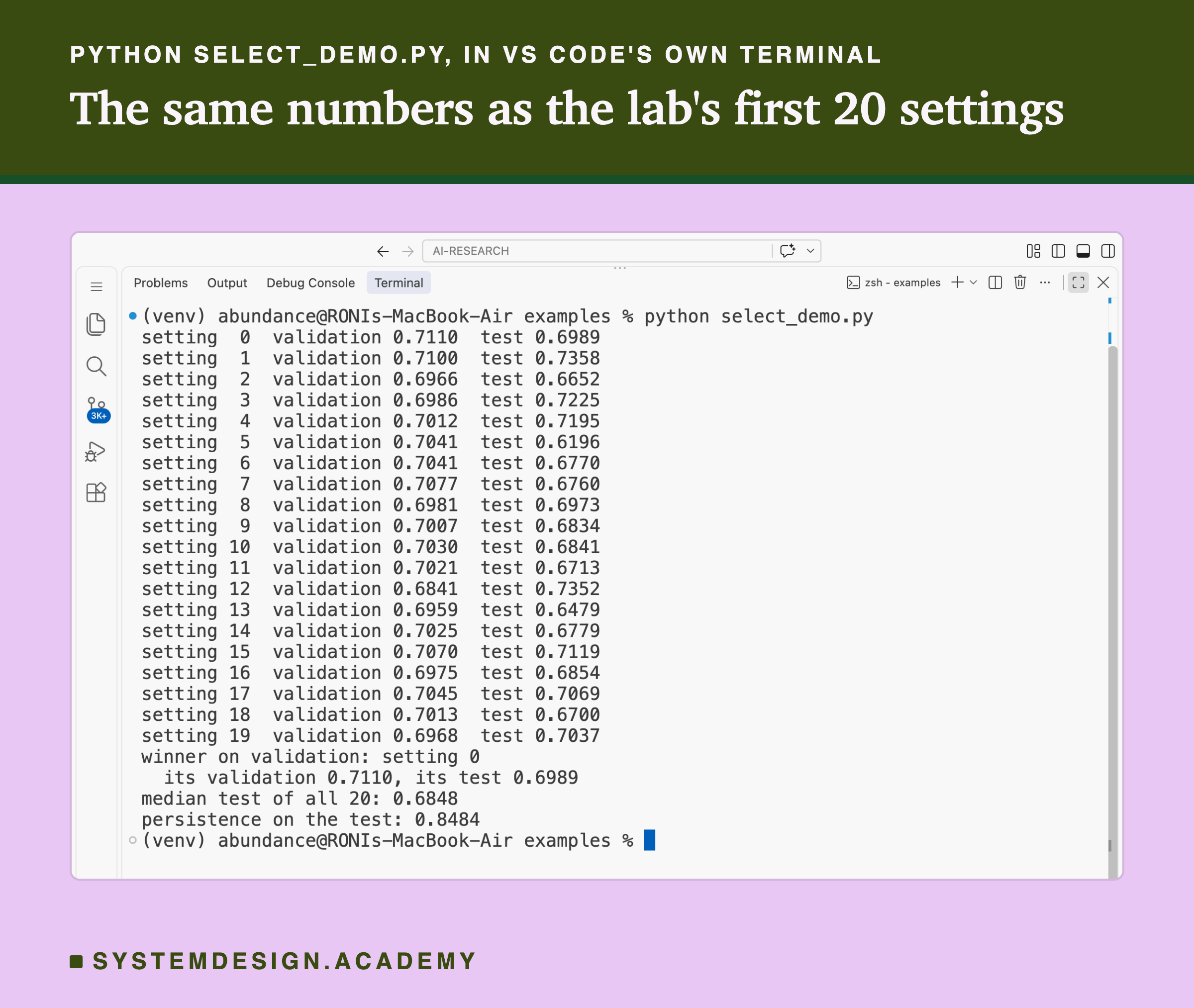
This script is the lab made small. It downloads the same data, draws the lab's first 20 settings with the same seed, trains each on the first 60%, and prints each setting's validation and test score. Then it prints the winner on validation, the median test score of the 20, and persistence on the same test. It does not need a GPU.

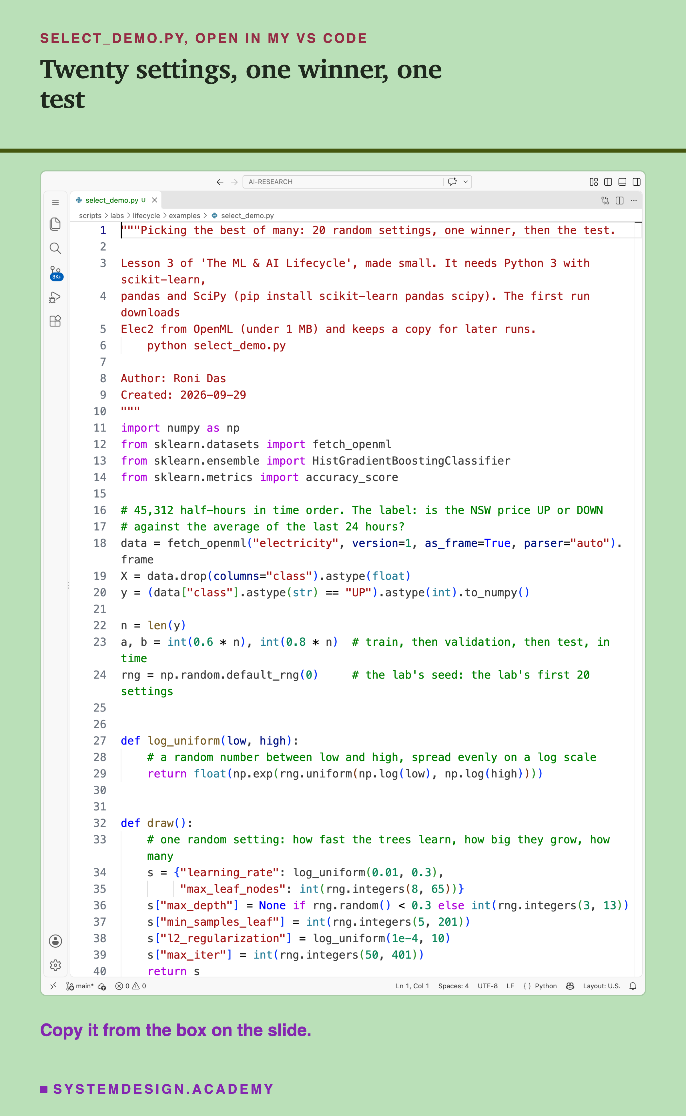
Before you run this lab. You need Python 3 and three libraries: pip install scikit-learn pandas scipy. scikit-learn holds the model, the scores and the download; pandas holds the table; SciPy is the library the lab's report uses for the rank correlations, and scikit-learn needs it anyway. The first run downloads Elec2 from OpenML (under 1 MB compressed), so it needs an internet connection once; scikit-learn keeps a copy in a folder in your home directory (scikit_learn_data) for later runs. I ran it with scikit-learn 1.9.1 on a Mac. scikit-learn runs the same way on Windows and Linux, but I have not checked the numbers there, and another version of scikit-learn may give different decimals.

"""Picking the best of many: 20 random settings, one winner, then the test.

Lesson 3 of 'The ML & AI Lifecycle', made small. It needs Python 3 with scikit-learn,
pandas and SciPy (pip install scikit-learn pandas scipy). The first run downloads
Elec2 from OpenML (under 1 MB) and keeps a copy for later runs.
    python select_demo.py

Author: Roni Das
Created: 2026-09-29
"""
import numpy as np
from sklearn.datasets import fetch_openml
from sklearn.ensemble import HistGradientBoostingClassifier
from sklearn.metrics import accuracy_score

# 45,312 half-hours in time order. The label: is the NSW price UP or DOWN
# against the average of the last 24 hours?
data = fetch_openml("electricity", version=1, as_frame=True, parser="auto").frame
X = data.drop(columns="class").astype(float)
y = (data["class"].astype(str) == "UP").astype(int).to_numpy()

n = len(y)
a, b = int(0.6 * n), int(0.8 * n)  # train, then validation, then test, in time
rng = np.random.default_rng(0)     # the lab's seed: the lab's first 20 settings


def log_uniform(low, high):
    # a random number between low and high, spread evenly on a log scale
    return float(np.exp(rng.uniform(np.log(low), np.log(high))))


def draw():
    # one random setting: how fast the trees learn, how big they grow, how many
    s = {"learning_rate": log_uniform(0.01, 0.3),
         "max_leaf_nodes": int(rng.integers(8, 65))}
    s["max_depth"] = None if rng.random() < 0.3 else int(rng.integers(3, 13))
    s["min_samples_leaf"] = int(rng.integers(5, 201))
    s["l2_regularization"] = log_uniform(1e-4, 10)
    s["max_iter"] = int(rng.integers(50, 401))
    return s


scores = []
for k in range(20):
    model = HistGradientBoostingClassifier(early_stopping=False, random_state=0,
                                           **draw())
    model.fit(X[:a], y[:a])                               # learn: first 60%
    val = accuracy_score(y[a:b], model.predict(X[a:b]))   # choose: next 20%
    test = accuracy_score(y[b:], model.predict(X[b:]))    # judge: last 20%
    scores.append((val, test))
    print(f"setting {k:>2}  validation {val:.4f}  test {test:.4f}")

win = max(range(20), key=lambda k: scores[k][0])   # the best on validation
print(f"winner on validation: setting {win}")
print(f"  its validation {scores[win][0]:.4f}, its test {scores[win][1]:.4f}")
print(f"median test of all 20: {np.median([t for _, t in scores]):.4f}")
print(f"persistence on the test: {(y[b - 1:-1] == y[b:]).mean():.4f}")

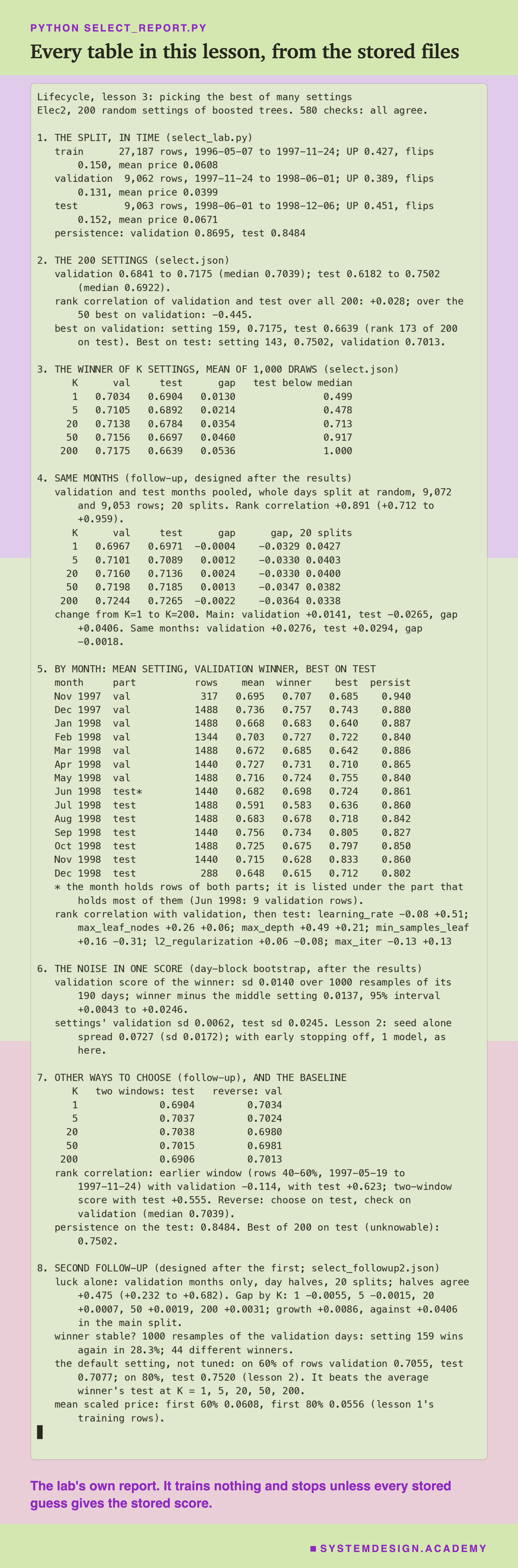
The report lives in scripts/labs/lifecycle/select_report.py. It reads the lab's stored file, results/select.json, the follow-up's results/select_followup.json, lessons 1 and 2's stored files, and the Elec2 labels from scikit-learn's local copy. It trains nothing. The follow-up stored every setting's guesses on the validation and test rows, so the report recomputes every score from those guesses and the labels, and stops unless each one equals the stored score to twelve decimal places. It also replays the lab's 1,000 draws for every K with the same seed and stops unless it gets the stored numbers. It makes 453 checks in all, and they all agree. It changes nothing in the lab's files.

Its json mode writes every number to results/wc-report.json, which the figures read. The demo mode checks the student script's stored run, and the box mode writes the playground below and checks it.

What came before the run, in select_lab.py: the split, the ranges of the six settings, the 200 draws, the 1,000 selection draws per K, the rank correlation and the persistence line. What came after I saw the results: the same-months control, the two-window score and the reverse (the follow-up), and in the report the rank correlation of the top 50, the table by month, the correlations of each setting, the bootstrap, and the comparison with lesson 2.

This box has no model in it. It holds the real validation and test score of all 200 settings, and the same 200 models scored on the two halves of the same months, from the follow-up's first random split. It runs in your browser.

As it is, the box prints the rank correlation of validation and test, +0.028, the median test score, 0.6922, and persistence, 0.8484, then plays the tuning game 1,000 times for each K. The rank correlation and the K = 200 line are exactly the lab's, and the report's box mode checks that. The other lines use Python's own random draws instead of the lab's, so they land near the lab's numbers, not on them: within 0.0011 in my check.

Try curse(20, same_months=True) to play the same game when validation and test come from the same months. These are the first control's scores, split 1, which pools the test months and so understates luck. This split starts at a gap of about -0.03 at every K, because its two halves differ in difficulty, so compare the change from curse(1, same_months=True) to curse(20, same_months=True), not the gap itself. Try curse(5) against curse(200), and rank_corr(SAME_VAL, SAME_TEST). Then try a different seed, curse(20, seed=7), and see how much one set of 1,000 draws moves.

Loading. fetch_openml("electricity", version=1) downloads Elec2 once and reads the local copy after that. The label column holds the words UP and DOWN, turned into 1 and 0. The eight inputs become plain numbers with astype(float), as in the lab.

The two cuts. a is 60% of the rows, 27,187, and b is 80%, 36,249. Training is everything before a, validation is from a to b, and test is from b to the end. Nothing is shuffled.

The random settings. rng = np.random.default_rng(0) is the lab's random generator with the lab's seed, so the script draws exactly the lab's first 20 settings. log_uniform picks a number evenly on a log scale, so a value between 0.01 and 0.03 is as likely as one between 0.1 and 0.3. draw asks for the six values in the lab's order; the order matters, because each call takes the next numbers from the generator.

The loop. Each setting builds a fresh HistGradientBoostingClassifier with early_stopping=False and random_state=0, learns from the first 60%, and is scored on validation and on test. Both scores are printed, one line per setting.

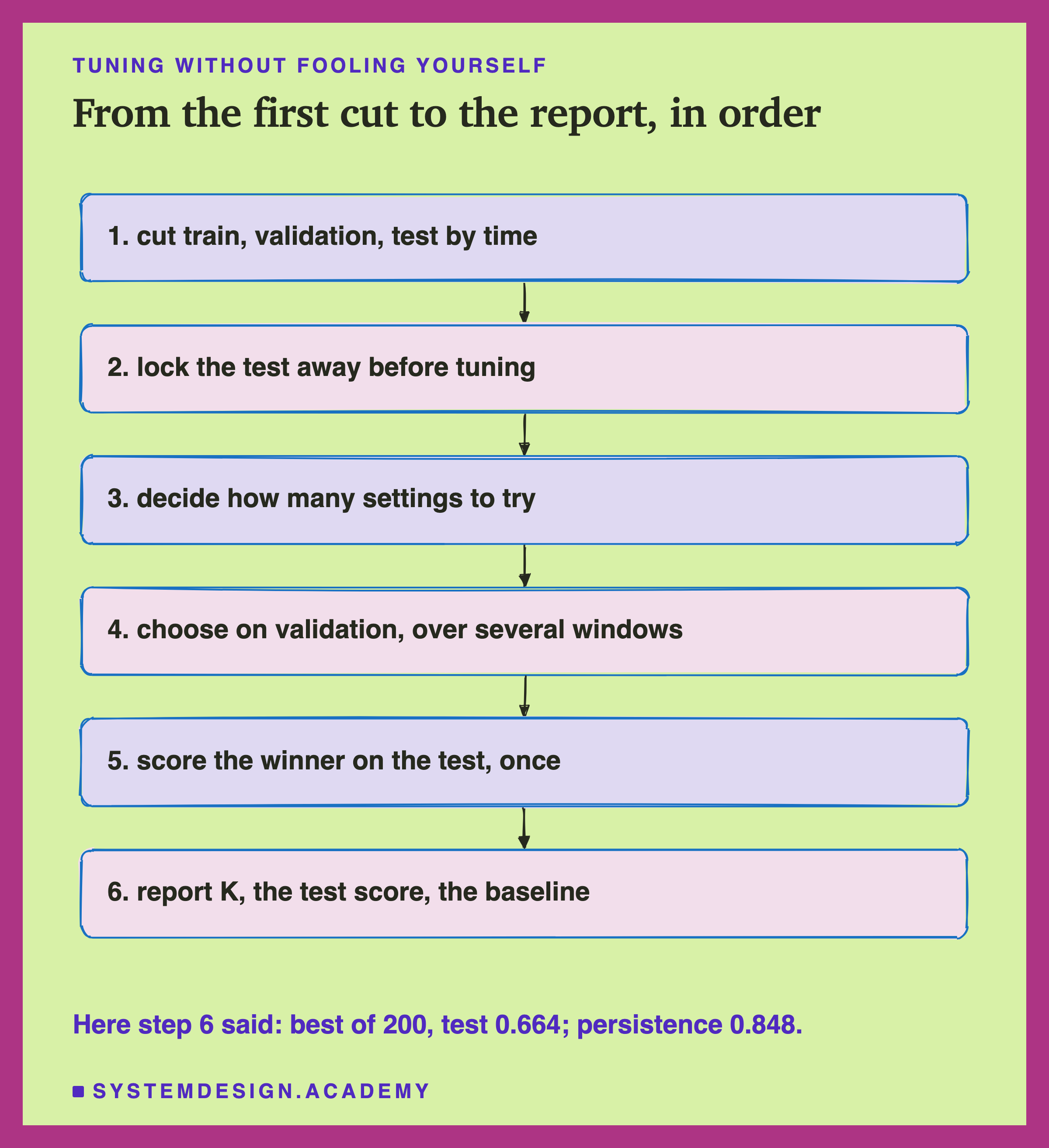
Cut the data by time, into three parts. If rows arrive in time order, train on the oldest, choose on the next, and judge on the newest, the way the model will be used.

Lock the test away before you start. Decide which rows are the test before you look at any score, and do not look at the test again until the choice is final.

Decide how many settings to try, and write it down. There is no safe number; here a winner of 5 already did no better on test than a random pick. Every extra setting is another chance for a lucky or ill-suited winner.

Choose on more than one window. For data in time order, score each setting on two or more later windows and average them. Check that the windows agree: if the rank correlation between them is near zero or below, as it was here between the earlier window and validation (-0.11), the choice means little. The playground below lets you check the orders yourself.

Score the winner on the test, once. That is the number to report.

Report K, the winner's test score and the baseline together. "Best of 200, test 0.664, persistence 0.848" tells a reader far more than "validation 0.718".

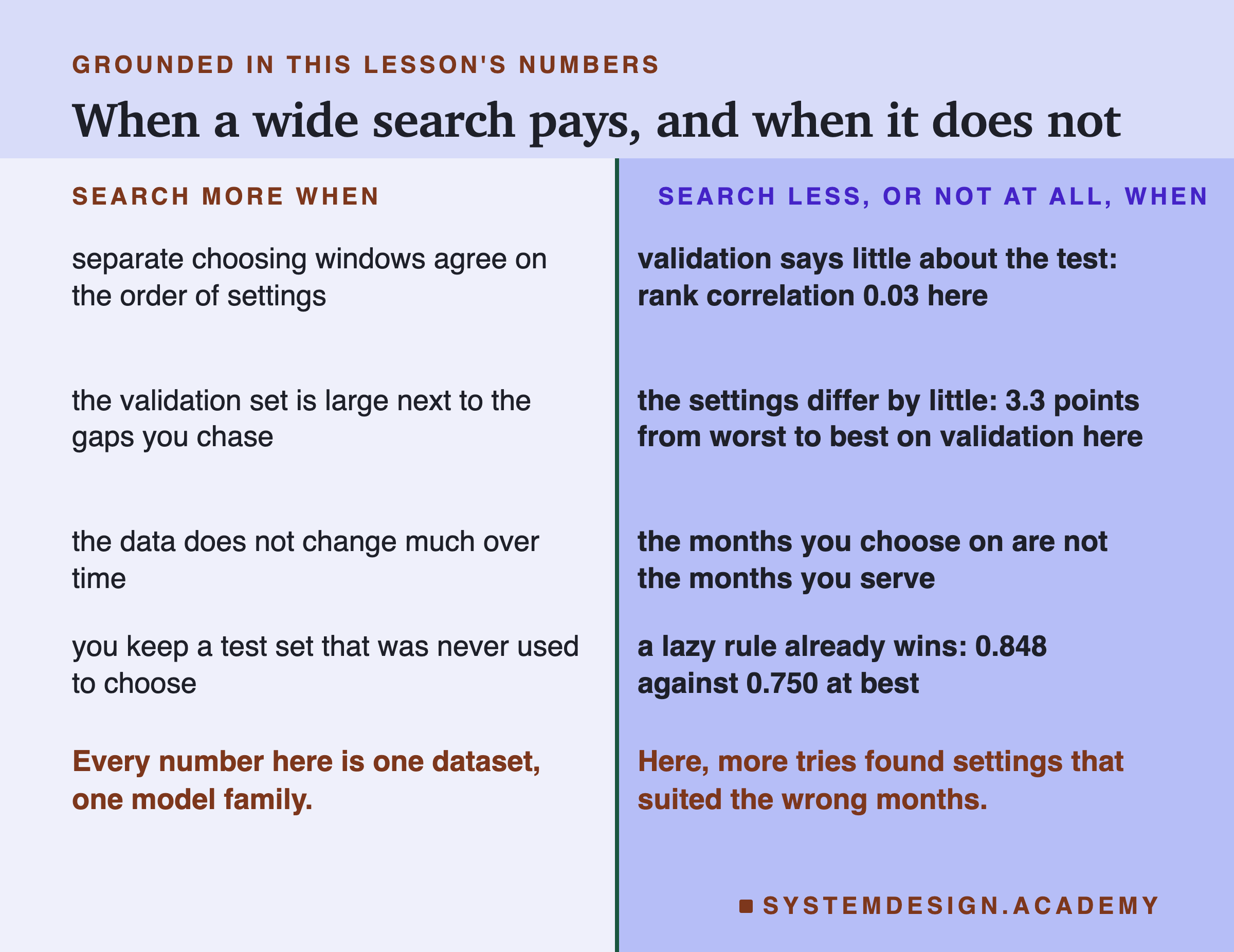
Use a wide search when the choosing rows are like the serving rows. In the same-months control, validation and test agreed (rank correlation 0.89) and the winner's test score rose with K, from 0.697 to 0.727. There, more tries really helped.

Use it when the settings differ by more than the noise. A setting that is ten points better will almost always win, however noisy the scores are. A setting that is half a point better will often lose to luck.

Use it when you keep a clean test set. Then even a bad search is caught before it ships, as it was here.

Do not search widely when the data drifts and you choose on one window. Here the best of 200 came 173rd of 200 on the future.

Do not search widely when the settings barely differ. Here all 200 spanned 3.3 points on validation. A search over settings that close is mostly a search over noise and over the quirks of the validation months.

Check the baseline before a wide search. If a rule with no learning is far ahead, as persistence was here, a better setting will not close the gap; a better framing or better inputs might.

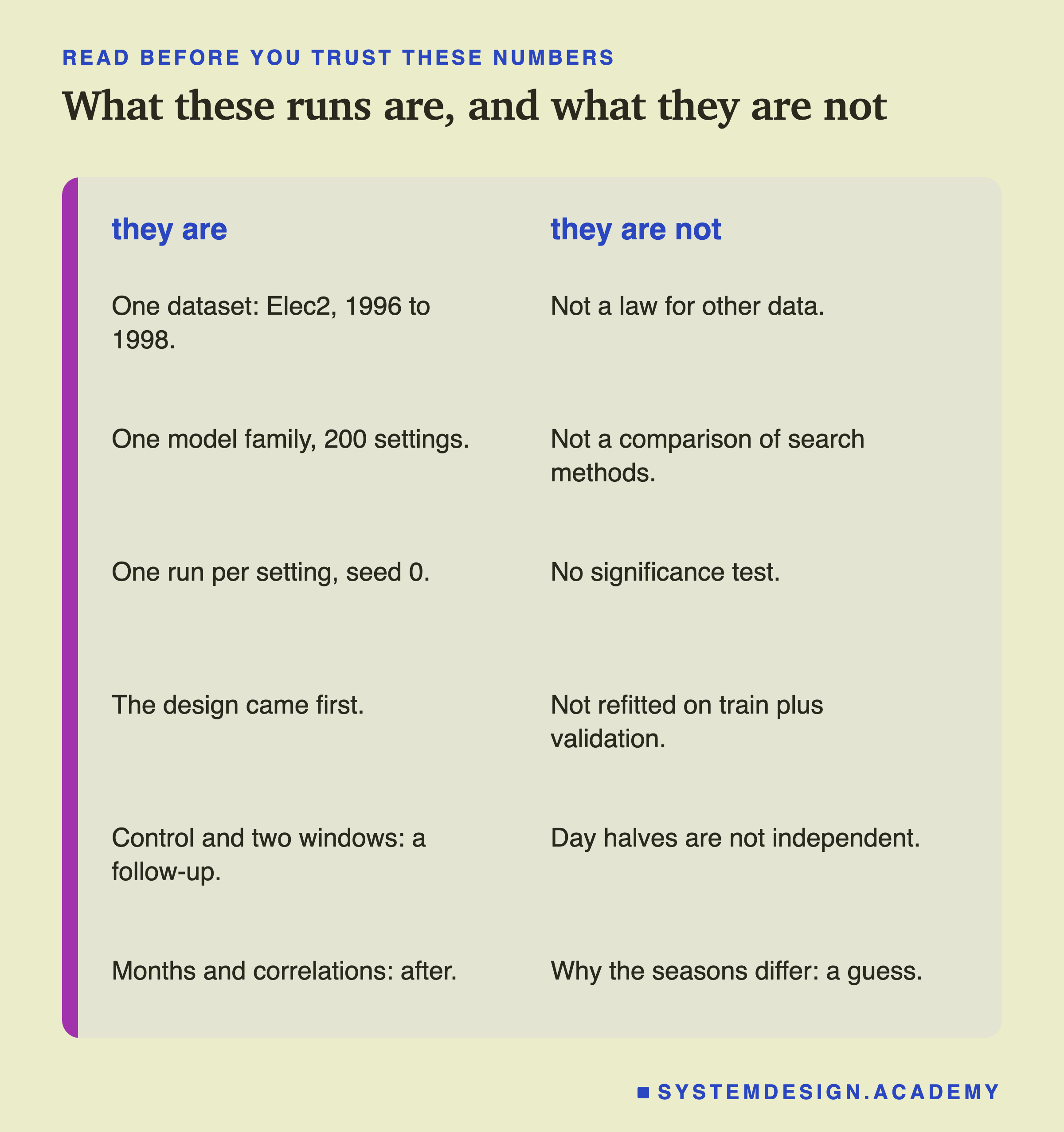
One dataset, one model family. Everything here is boosted trees on Elec2, with one split in time. Here luck alone was about a fifth of the growth, 0.9 of 4.1 points. On data that does not drift, luck may be most of it. I have not tested other data.

Random search only. The lab drew settings at random. Smarter search methods, which pick the next setting based on the last ones, were not tested, and this is not a comparison of them.

The winner was not retrained. In practice many teams retrain the winning setting on training plus validation rows before testing it. The lab scored the model trained on the first 60%, as its design said. A retrained winner might score differently.

Design first, follow-up after. The lab's design was written before it ran. The same-months control, the two-window score and the reverse are a follow-up, designed after I saw the main results. The top-50 correlation, the month table, the setting correlations and the bootstrap were measured after the results. The second follow-up, the luck control within the validation months, the resampled winners and the untuned default, was designed after the first follow-up, prompted by a review. The controls' day halves come from neighbouring days, so they are more alike than truly new data and may understate luck, and the first control also pooled the test months' real differences into both halves.

Guesses stay guesses. Why the test months rewarded faster learning rates is my guess, and I have not tested it. The effect of leaving early stopping on is a reasoned expectation from lesson 2's numbers, not something this lab ran.

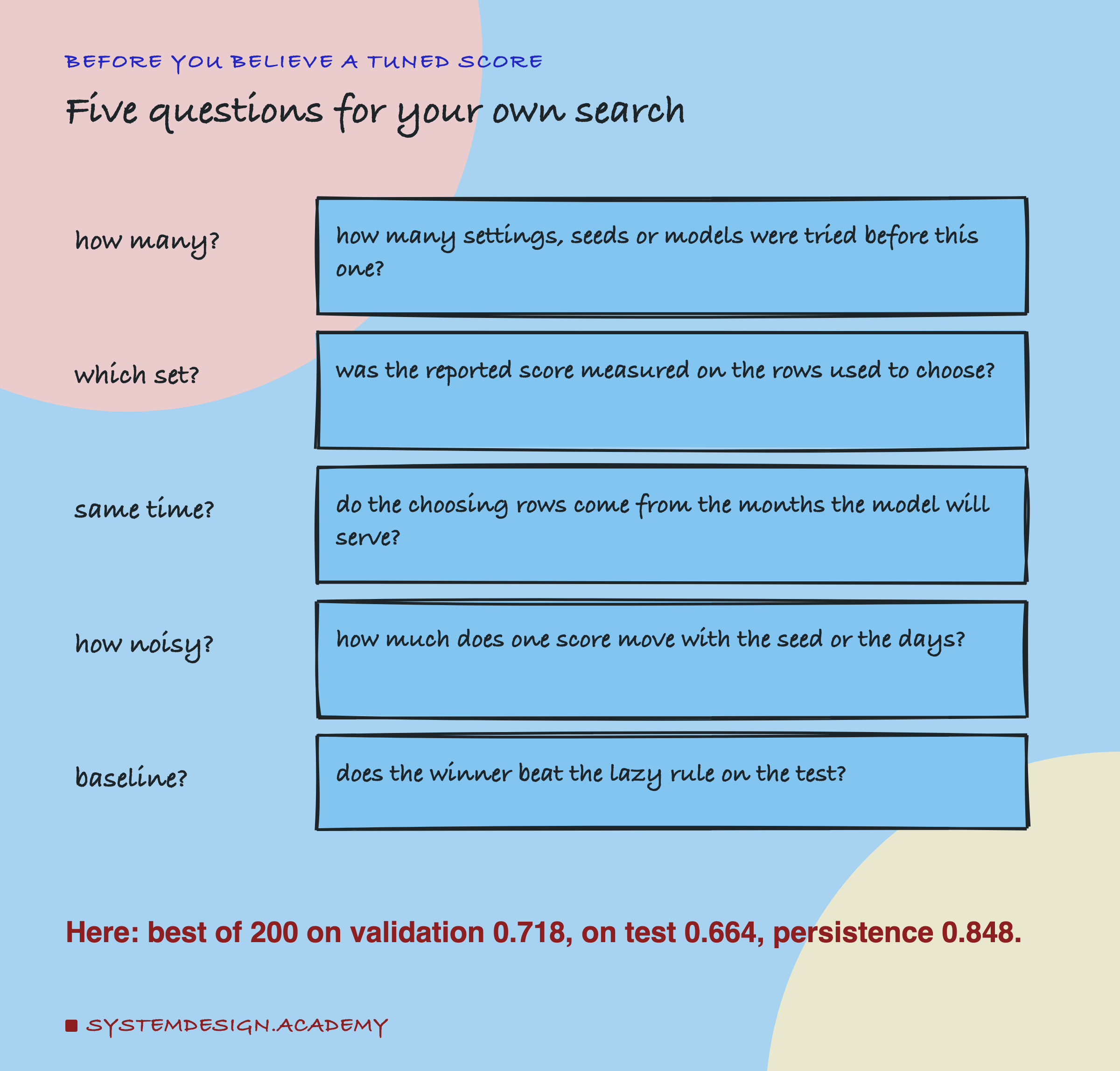
Find the last model your team tuned and ask the five questions on the card. The first two are usually answered by the experiment tracker: count the runs, and check which rows the reported score came from. If the reported score is the validation score of the best run, you do not yet know how good the model is. Score it once on rows nobody chose with.

Then check the third question with a small version of this lab: score your top few settings on two different windows of your validation data, and see if they come out in the same order. If they do not, the choice between them is not telling you much, and a wider search will not fix that.

The next lesson planned for this chapter moves from choosing a model to promoting one: the gate a pipeline uses to decide whether a newly trained model replaces the one in use, and how often a model that is no better gets through.