Let me start at an airport.

Outside the terminal, a small shuttle bus takes people to the hotels. It has 20 seats. The driver has one rule: leave when all 20 seats are full, or 10 minutes after the first person sits down, whichever comes first.

Think about what this rule does. On a busy evening the bus fills in two minutes and leaves. One trip carries 20 people for about the cost of driving one. Without the rule, the driver would make 20 trips, and a long line would form at the door.

On a quiet morning it is different. The first person sits down and waits. Nobody else comes. After 10 minutes the bus leaves with one person in it. That person waited 10 minutes for nothing, and the trip cost the same as a full one.

There is a third way to run the bus. The driver does not wait at all. When the bus comes back, everyone standing at the door gets on, and it leaves at once. On a quiet morning it leaves with one or two people. On a busy evening it leaves full, because people gathered while it was away.

A prediction service can follow the same kinds of rules. Instead of asking the model for one answer at a time, it can collect several requests and ask the model once for all of them. In this lesson I build those rules into a real service and measure both sides: how much work they save, and how long they make people wait.

This is lesson 4 of the chapter on serving a model. Lesson 2, latency anatomy, took one request apart and found that the model's predict_proba was the largest step. Lesson 3, tail latency, looked at the slowest requests. Both lessons sent one request at a time, so no request ever waited for another one.

This lesson lets requests overlap. Batching cannot work without this: a request can only share a model call with another request if both are waiting at the same moment.

I use the same model, the same service code and the same kind of rented machine as lessons 2 and 3, so I do not explain them again. In short: the model is the features chapter's gradient boosted tree model. It scores one customer of a real online shop at the start of a month, and it scored a test AP of 0.5450. The service is a small web service built with FastAPI and run by uvicorn, and it reads the customer's six features from SQLite. If any of that is new, please read lesson 2 first.

The question is short. Does batching help a small model that runs on a CPU, and what does it cost in latency? I answer it in two parts. Part A times the model alone, with no web server, on batches of different sizes. Part B puts a batcher inside the service and sends it real traffic.

Please read this slide slowly if any word is new. Every slide after it uses these words.

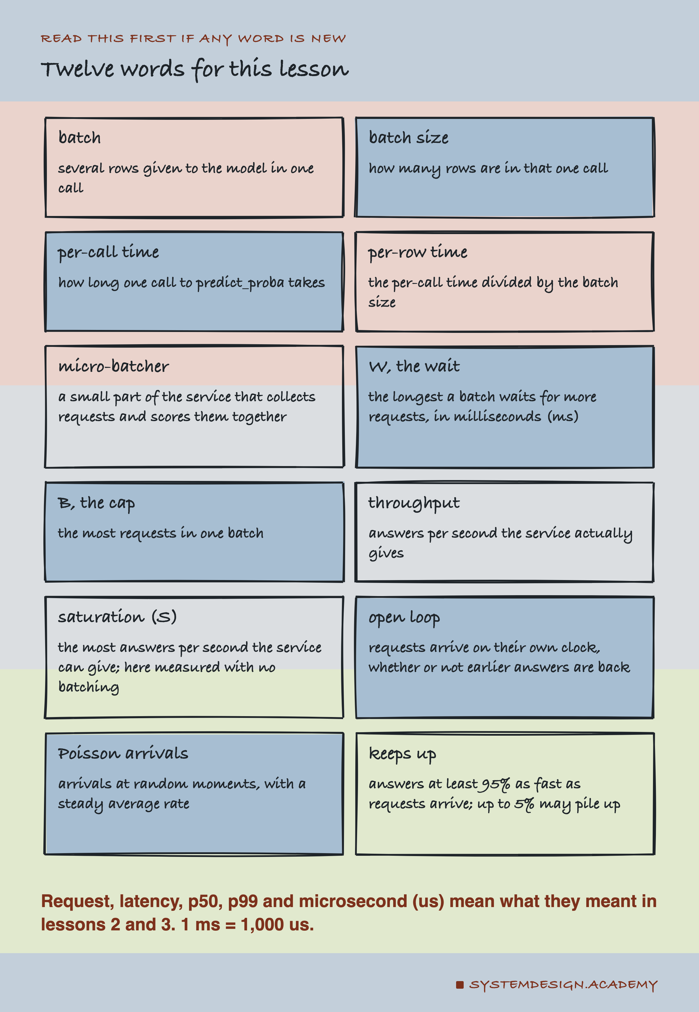
A batch is a group of rows given to the model in one call. Think of a photocopier. Copying one page means walking to the machine, lifting the lid, pressing start, and walking back. Copying ten pages costs the same walk and only a little more machine time. The walk is the fixed cost of a call. The machine time for each page is the per-row cost.

The batch size is how many rows are in one call. The per-call time is how long one call takes. The per-row time is the per-call time divided by the batch size.

A micro-batcher is a small part of the service that collects requests as they arrive and scores them together. Mine has two dials. B is the cap: the most requests in one batch, like the 20 seats of the shuttle. W is the wait: the longest the first request in a batch waits for more to come, like the 10 minutes. With W = 0, the batcher never waits on purpose. It takes whatever has gathered while it was busy, like the third way to run the bus.

Throughput is how many answers per second the service actually gives. Saturation is the most it can give. I call the saturation of the service with no batching S.

An open loop test sends requests on their own clock, like customers who walk in when they want, whether or not the shop is busy. Poisson arrivals are arrivals at random moments with a steady average rate. Sometimes three come almost together, sometimes there is a long gap. A service keeps up when it answers at least 95% as fast as requests arrive. So up to 5% of the requests may still pile up in a run that keeps up. If it answers slower than that, a queue grows and never empties.

Here is the main result first. Each line is one way of running the service. Each point is the p99 latency at one arrival rate, the median of five rounds. Latency is counted from the moment a request arrived, so every kind of waiting counts.

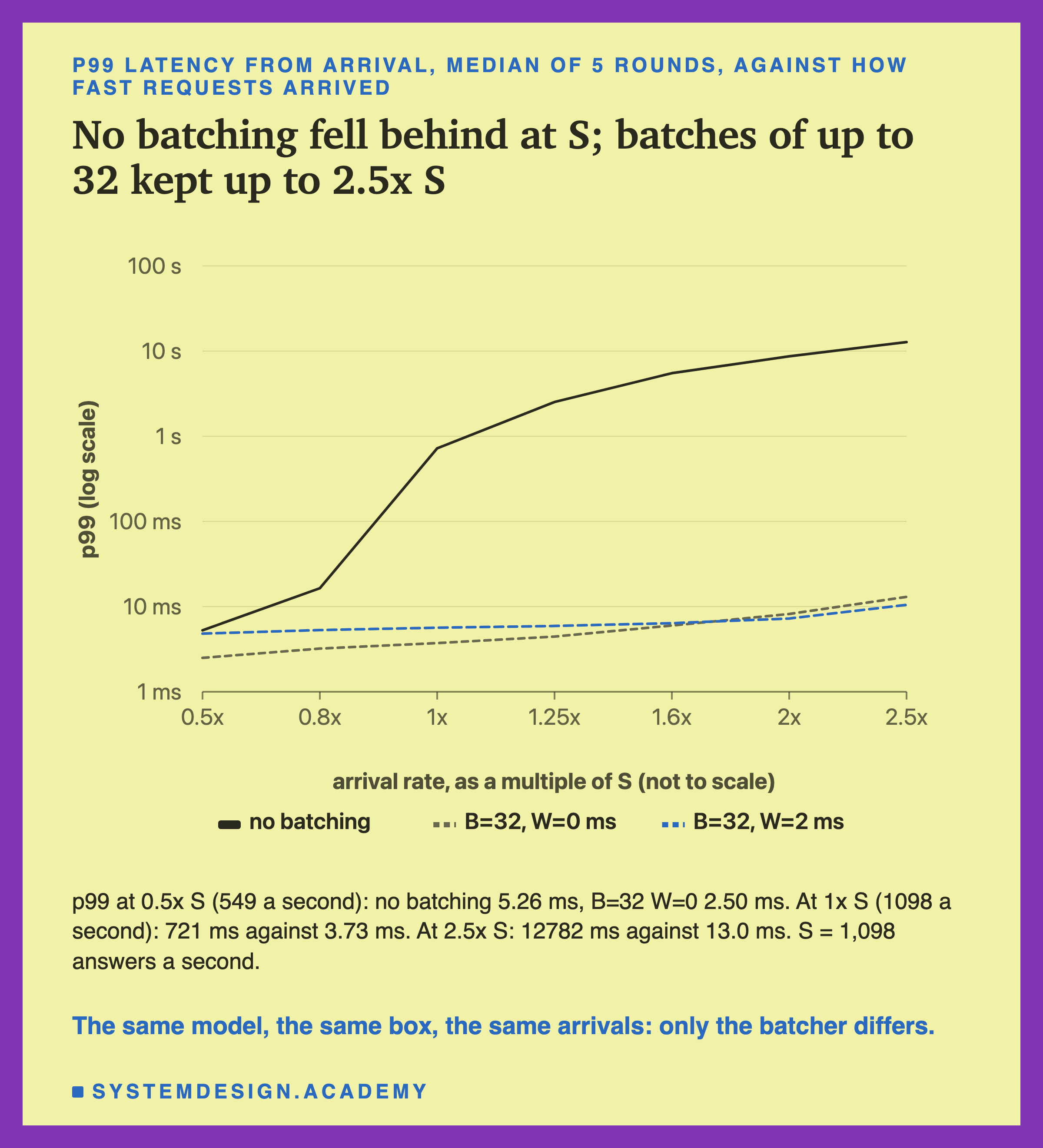
With no batching, the service fell behind at S. At 1,098 arrivals a second its p99 was 721 milliseconds, and at 2.5 times that rate it was 12.8 seconds. Its queue never emptied, so those numbers only grow if the test runs longer.

With batches of up to 32 and no timed wait, the service kept up at every rate I tried, up to 2,746 arrivals a second. Its p99 stayed between 2.50 ms and 13.0 ms.

Even at half of S, that batcher cut the p99 in half, from 5.26 ms to 2.50 ms. I did not expect that, and a later slide explains it.

A timed wait cost latency at a low rate. With W = 2 ms the median was 3.11 ms against 1.18 ms. Its p99 (4.82 ms) was still lower than no batching's, but higher than W = 0's 2.50 ms.

So for this small model on one core, batching helped a lot, and the setting with no timed wait was the safe choice at every rate. The rest of the lesson shows where those numbers come from.

I wrote the lab's design into the docstring of scripts/labs/serving/batching_requests.py on 2026-10-04, before any timed run. It names every measurement, every setting, the rule for "told apart from noise", and eleven guesses.

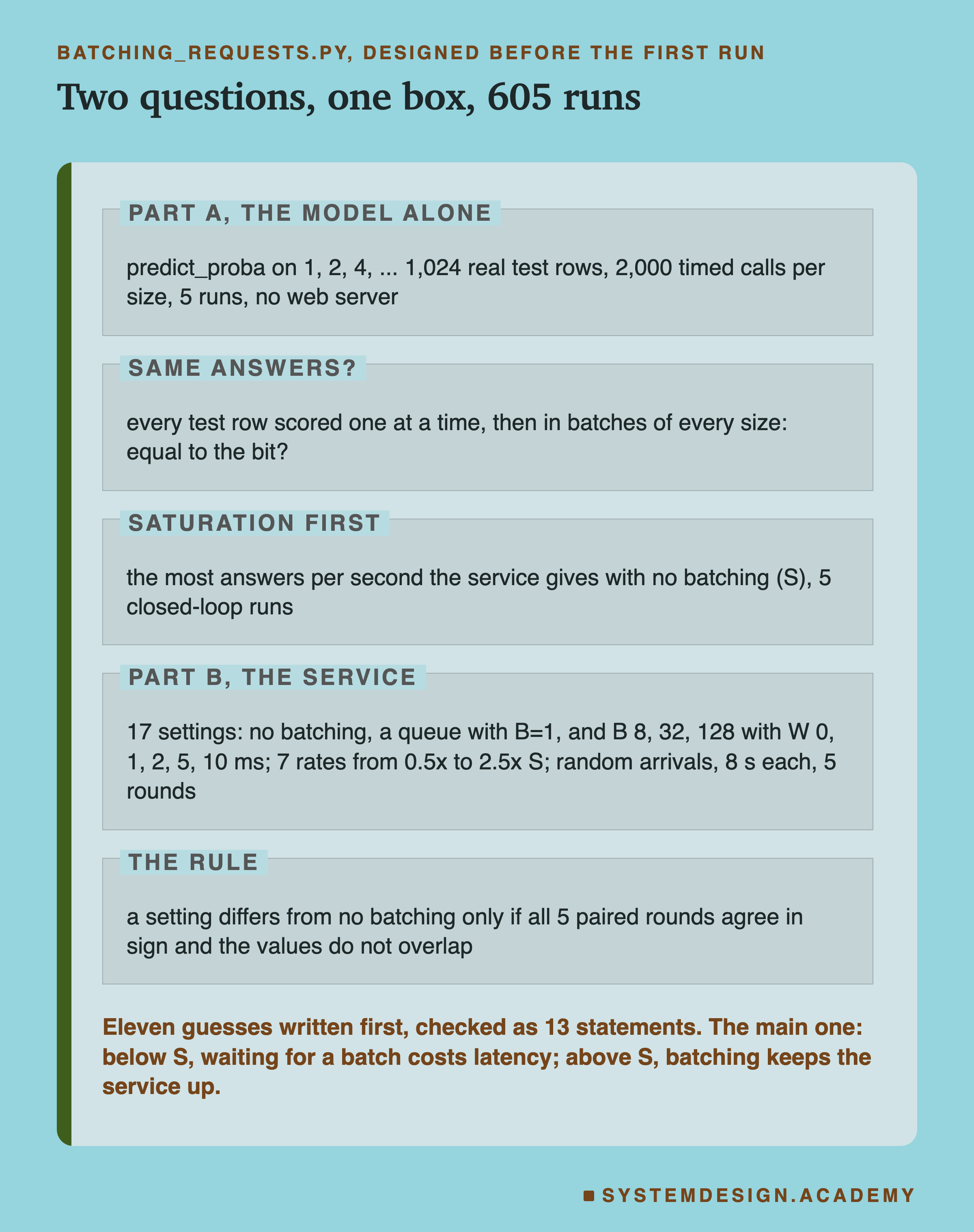
Part A times predict_proba alone, with no web server, on batches of 1, 2, 4 and so on up to 1,024 real test rows. Each size gets 2,000 timed calls, and the whole thing runs five times, each time in a fresh Python process with the sizes in a new random order.

The saturation runs find S. Sixteen connections each send a new request the moment their last answer arrives, for 8 counted seconds, with no batching. This is a closed loop: the client waits for answers before sending more, so it measures the most the service can do.

Part B puts the batcher in the service. It tries 17 settings. None is lesson 2's handler, which scores its one row itself. A queue with B = 1 sends every request through the batcher machinery but never groups two, so it measures what the machinery alone costs. The other 15 are B = 8, 32 or 128 with W = 0, 1, 2, 5 or 10 ms. B = 1 with a W above 0 would make no sense: a batch of one is full the moment its only request arrives, so it never waits.

Each setting meets seven arrival rates: 0.5, 0.8, 1, 1.25, 1.6, 2 and 2.5 times S. Each run lasts 8 seconds of arrivals and starts a fresh service, and there are five rounds. Inside a round the 119 runs go in a shuffled order. So I can compare each setting with no batching on the very same traffic, round by round.

Like lessons 2 and 3, every timing comes from a small machine I rented from Amazon Web Services. None comes from my laptop, which is always busy with other work.

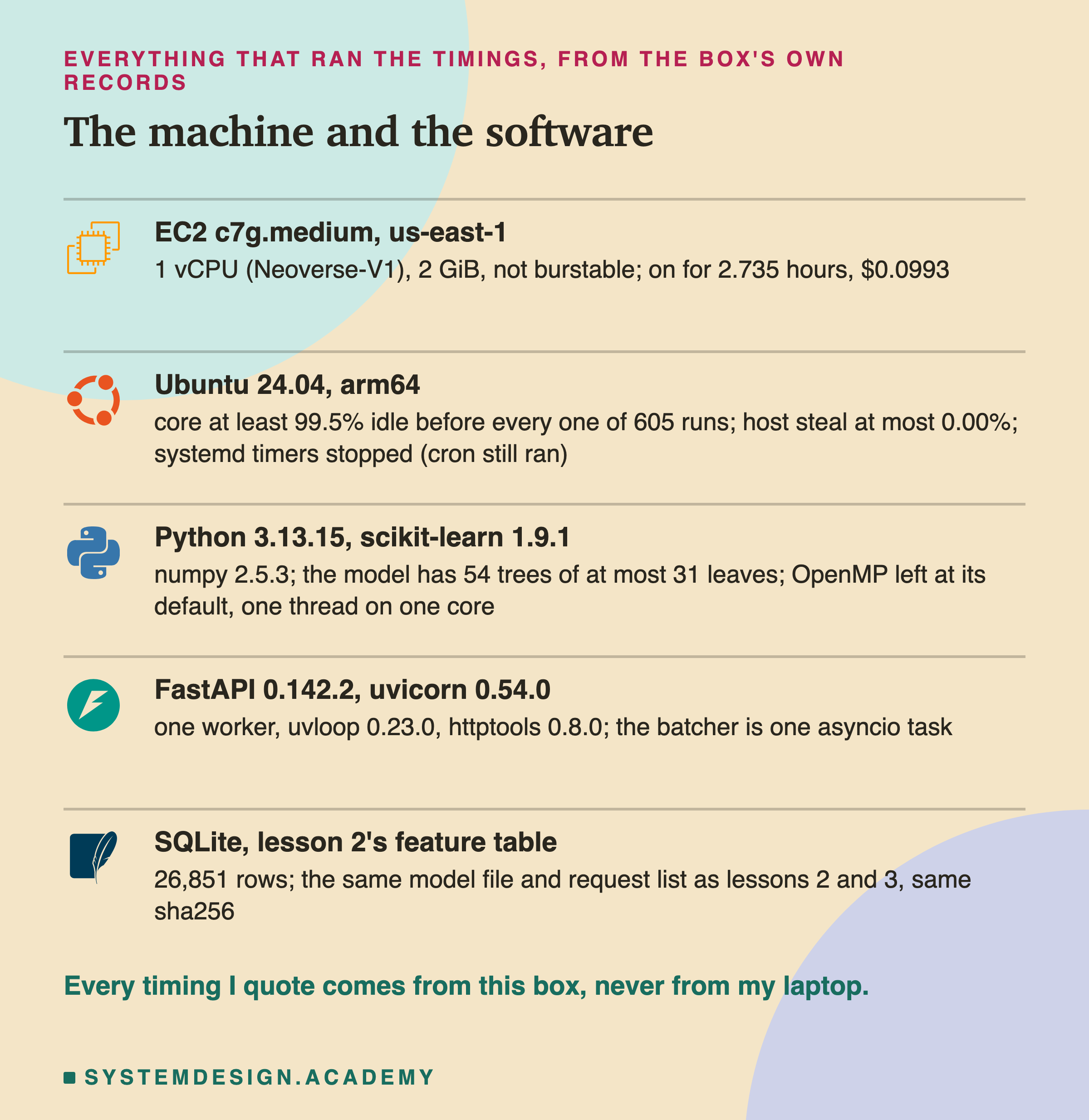
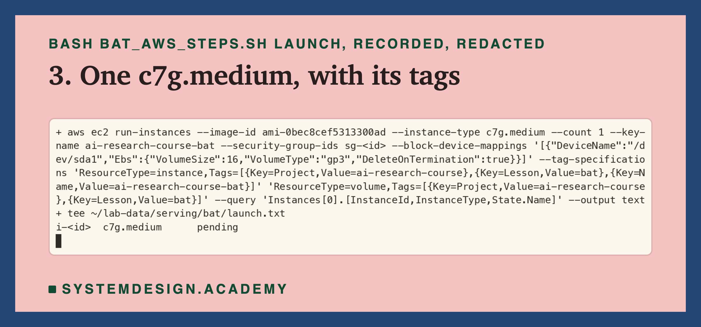
The box is an EC2 c7g.medium. AWS's own API lists it with 1 virtual CPU, 2,048 MiB of memory and no bursting, and its AWS page says C7g instances use Graviton3 processors. My account allows only one of these at a time, so, as in lessons 2 and 3, the client and the service share that one core.

That matters more here than before. In lessons 2 and 3 the client sent one request and waited. Here the client sends requests on its own clock, so it works at the same moments the service does. Every request costs some core time in the client too. So S, the most the service answered with no batching, is really "the most the service and its client together could do on one core". The client's work per request is the same in every setting, so the comparisons between settings are fair. But the absolute numbers are lower than a service would reach with its client on another machine.

Three words from the figure. Steal is time the physical machine under my rented box gives to other customers' boxes; it was 0.00% in every run. OpenMP is a library that lets a program split work across several cores; scikit-learn uses it inside predict_proba, and on one core it uses one thread. An asyncio task is one job inside Python's asyncio system, which runs many small jobs on one thread by switching between them while each waits.

Before every run, the core had to be at least 95% idle over two seconds. I did not wait for the one-minute load average to fall, as lesson 3 did, because it takes minutes to decay and there were 605 runs. The load is still recorded before and after every run.

Before the recordings, here is the whole lab as one numbered sequence. The numbers on the arrows match the numbers on the recordings that follow.

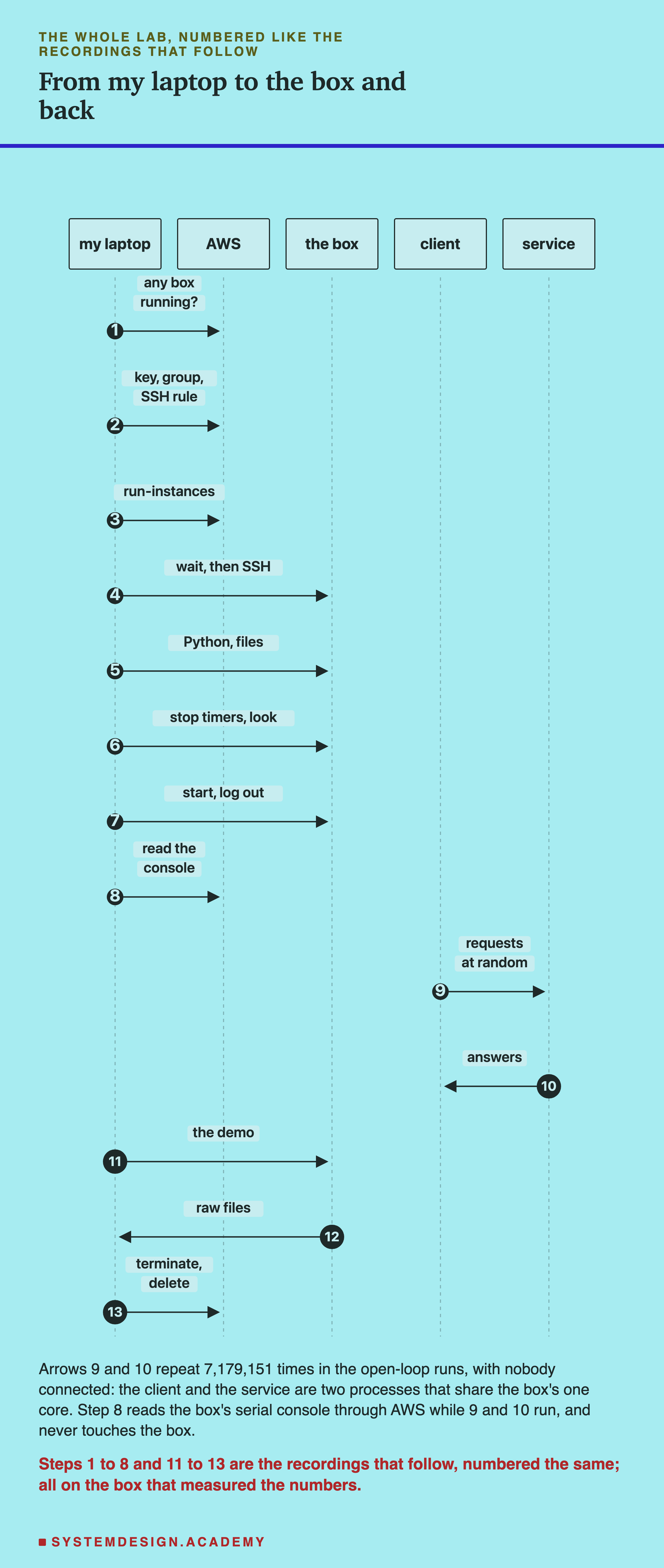
Steps 1 to 7 happen once: check, rent the box, set it up, and start the schedule. Step 8 is how I watched the schedule without touching the box. Arrows 9 and 10 are the timed work, millions of times, with nobody logged in. Steps 11 to 13 come after the schedule: the student demo, the copy of the results back to my laptop, and the deletion of everything.

Is anything pinned to the core? No. With one core there is nothing to choose. The client's two threads and the service take turns on it, and the operating system switches between them. That switching is part of every latency here, in every setting alike.

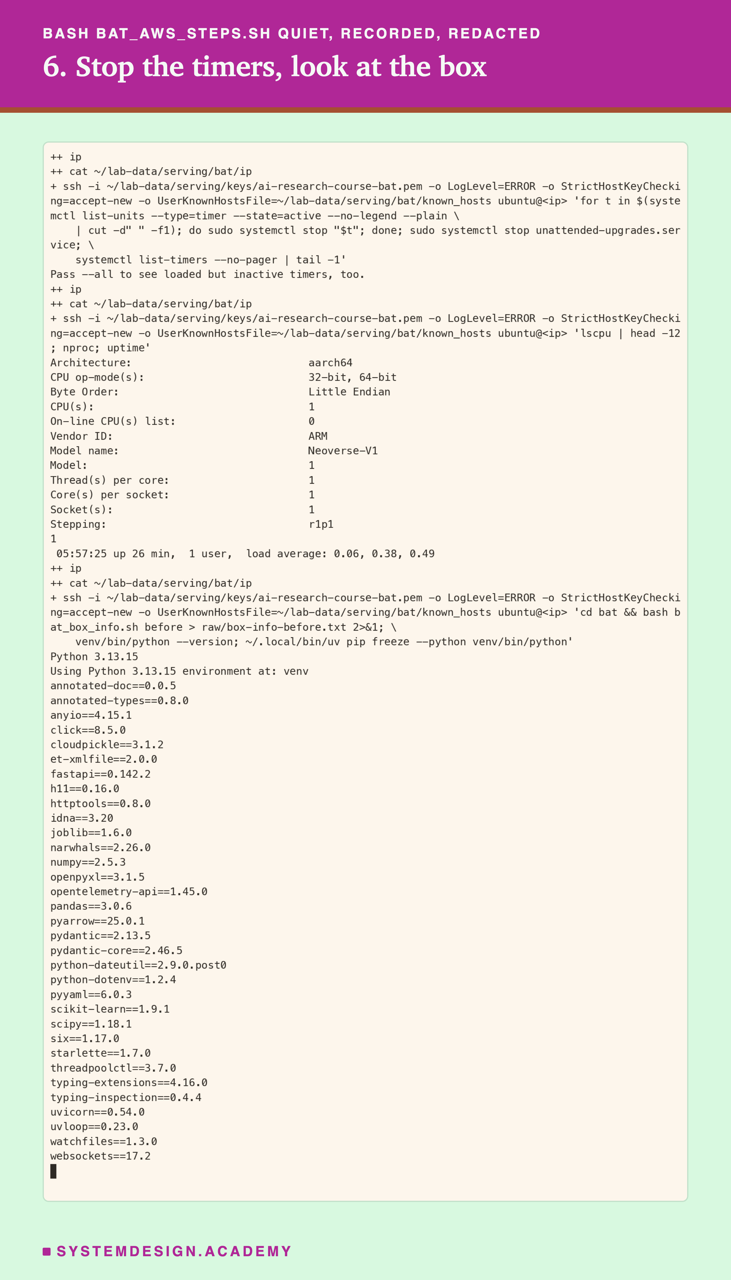
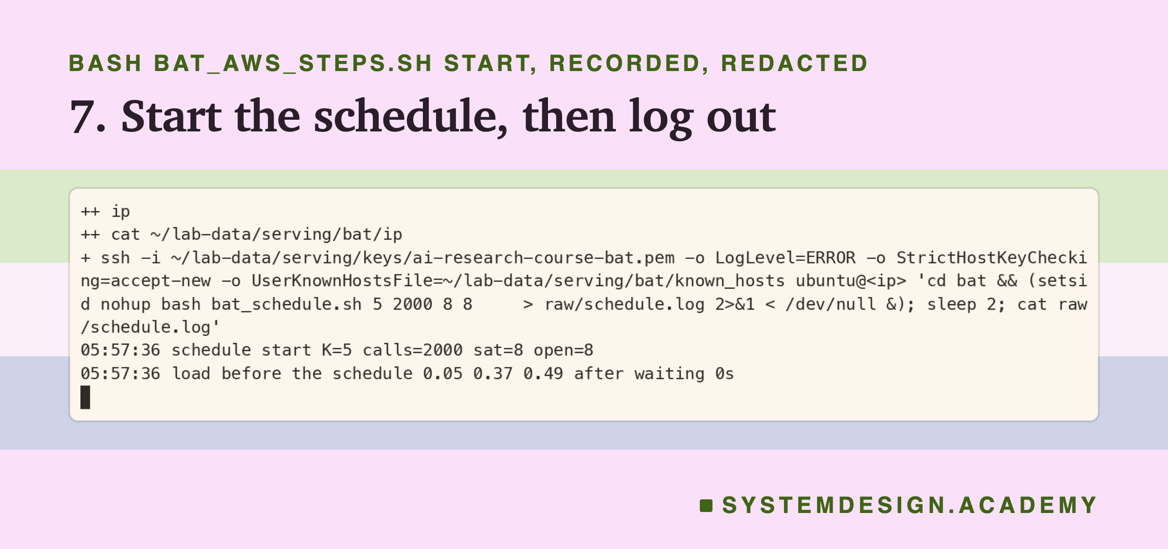
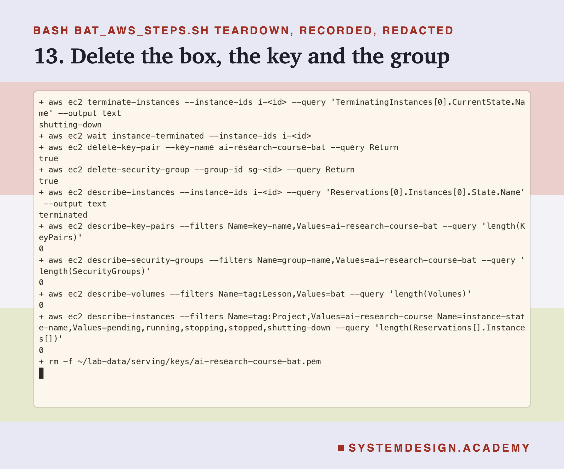
The rented box is part of the lab, so I show every step of it. You can rent the same kind of box and run the same schedule. The flow figure numbers the steps, and each recording below carries the same number.

Which box you see. Every recording comes from the box that measured this lesson's numbers. I planned the order so that no recording happened during a timed run. Steps 1 to 7 come before the schedule. Step 8 reads the box from outside without logging in. Steps 11 to 13 come after the schedule finished.

The path to follow. All the steps live in one file, scripts/labs/serving/bat_files/bat_aws_steps.sh. From the scripts/labs/serving folder, run bash bat_files/bat_aws_steps.sh check, then access, launch, wait, copy, quiet, start and watch; after the schedule, demo, fetch and, at the end, teardown. The code blocks on these slides are that file's lines, copied exactly, so you can read what each step does. If you would rather paste them by hand, paste this variables block first, in the same terminal. Each step also saves the group id, the box's id and its address to a small file, so the steps work in separate terminals too.

Step 1: is any other course box running? My account allows one small box of this kind at a time, and another lesson may be using it. So the first command counts the course's boxes that are not yet deleted. It must print 0.

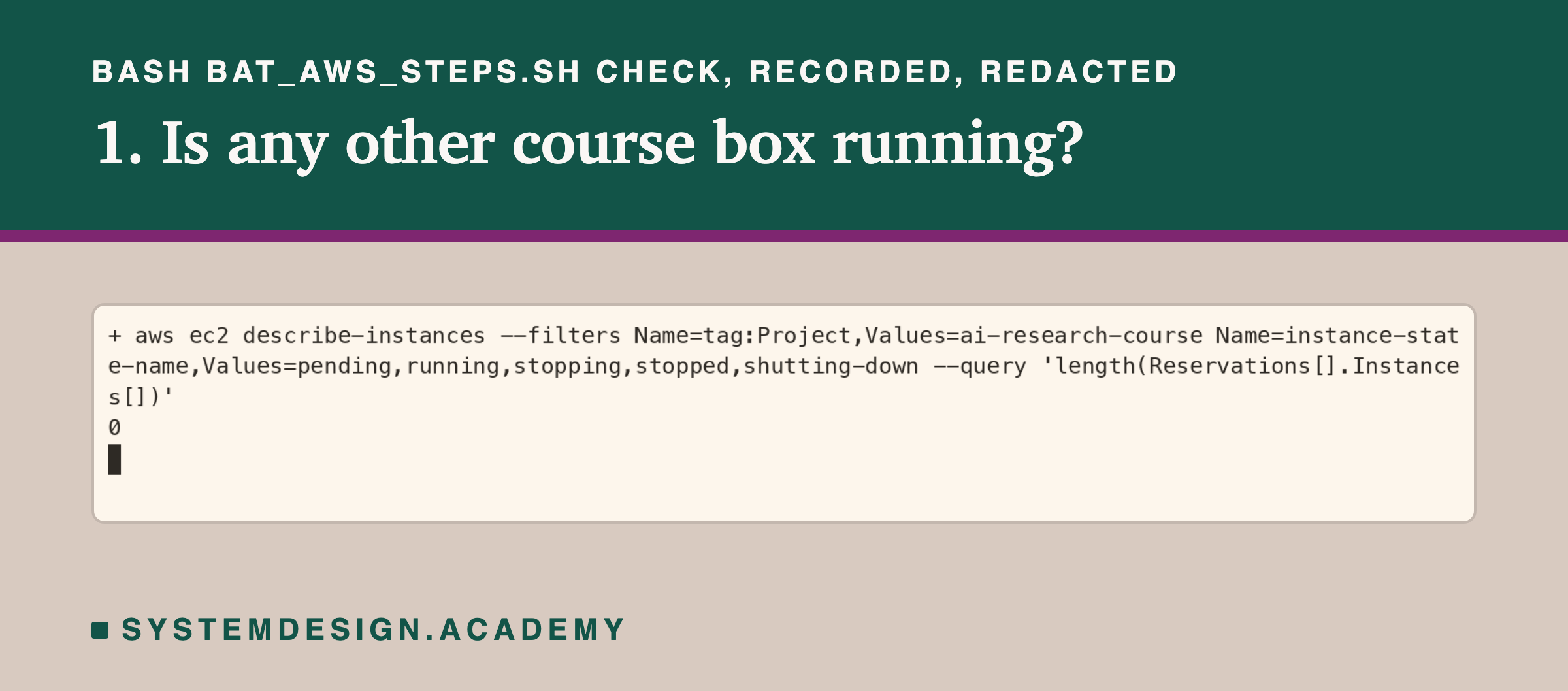
aws ec2 describe-instances --filters "Name=tag:Project,Values=ai-research-course" \
  "Name=instance-state-name,Values=pending,running,stopping,stopped,shutting-down" \
  --query "length(Reservations[].Instances[])"

Step 2: a key and a locked door. A key pair is how you prove to the box that you are allowed in. AWS keeps one half, and you keep the other half in a file that only you can read. A security group is a door rule for the box. Mine opens only port 22, the SSH port, and only to my own address.

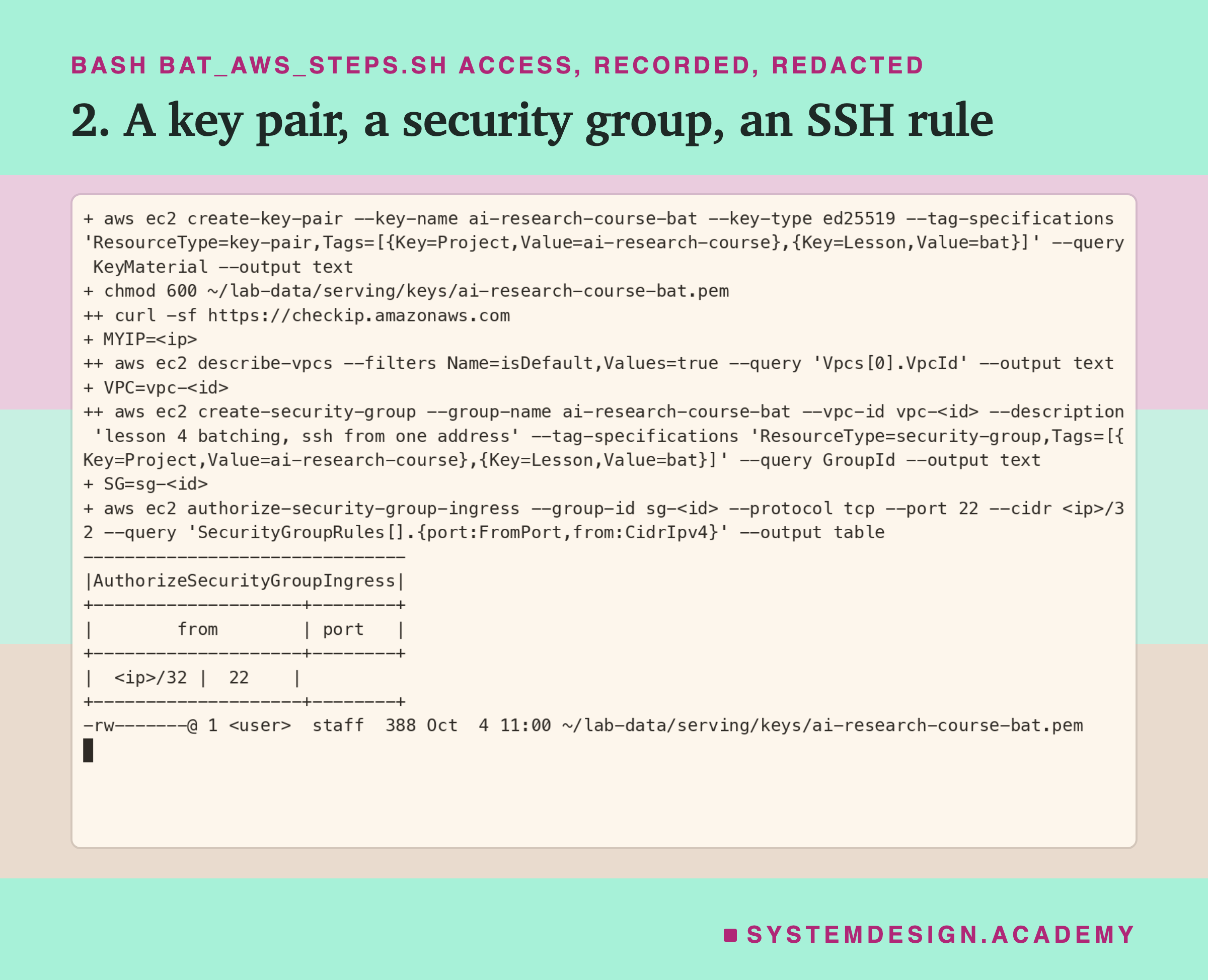
mkdir -p "$(dirname "$KEY")"
aws ec2 create-key-pair --key-name "$NAME" --key-type ed25519 \
  --tag-specifications "ResourceType=key-pair,Tags=[{Key=Project,Value=ai-research-course},{Key=Lesson,Value=bat}]" \
  --query KeyMaterial --output text > "$KEY"
chmod 600 "$KEY"
MYIP=$(curl -sf https://checkip.amazonaws.com)
VPC=$(aws ec2 describe-vpcs --filters Name=isDefault,Values=true --query "Vpcs[0].VpcId" --output text)
SG=$(aws ec2 create-security-group --group-name "$NAME" --vpc-id "$VPC" \
  --description "lesson 4 batching, ssh from one address" \
  --tag-specifications "ResourceType=security-group,Tags=[{Key=Project,Value=ai-research-course},{Key=Lesson,Value=bat}]" \
  --query GroupId --output text)
aws ec2 authorize-security-group-ingress --group-id "$SG" --protocol tcp --port 22 --cidr "$MYIP/32" \
  --query "SecurityGroupRules[].{port:FromPort,from:CidrIpv4}" --output table
echo "SG=$SG" >> "$STATE/vars"
ls -l "$KEY"

Keep the key file outside any git folder. Mine lives in , and the last step deletes it.

Step 4: wait until it runs. A new box takes a short while to start. The AWS tool can wait for you, and then the script tries SSH every five seconds until the box answers.

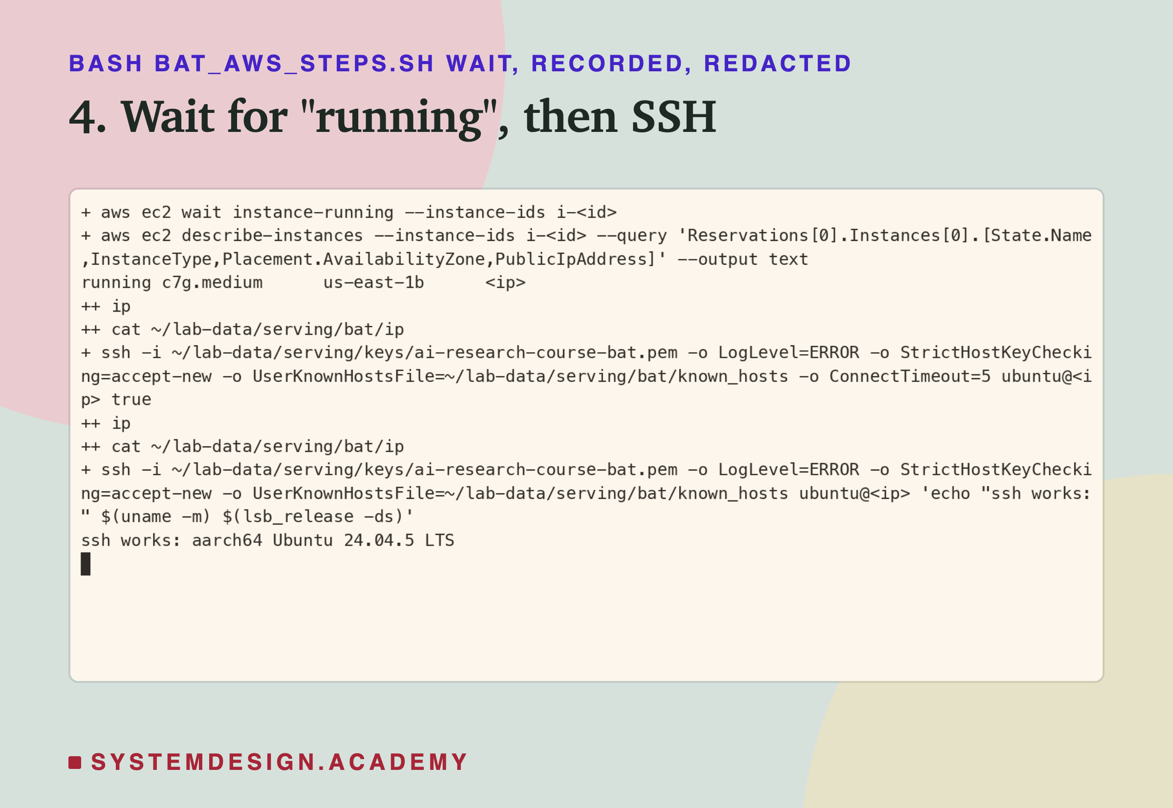
aws ec2 wait instance-running --instance-ids "$ID"
IP=$(aws ec2 describe-instances --instance-ids "$ID" \
  --query "Reservations[0].Instances[0].PublicIpAddress" --output text)
echo "IP=$IP" >> "$STATE/vars"
until ssh "${SSH[@]}" -o ConnectTimeout=5 ubuntu@"$IP" true 2>/dev/null; do sleep 5; done
ssh "${SSH[@]}" ubuntu@"$IP" 'echo "ssh works:" $(uname -m) $(lsb_release -ds)'

Step 5: Python and the lab files. The box gets the same Python, 3.13.15, and the same pinned library versions as lessons 2 and 3, through uv, a fast installer for Python. Then the lab files go over with scp, a copy command that works through SSH: lesson 2's model file, feature table, request list and service, this lesson's files, and the files the demo needs. The last command builds the SQLite table on the box and prints the files' sha256 fingerprints, so you can check they match the ones on your computer.

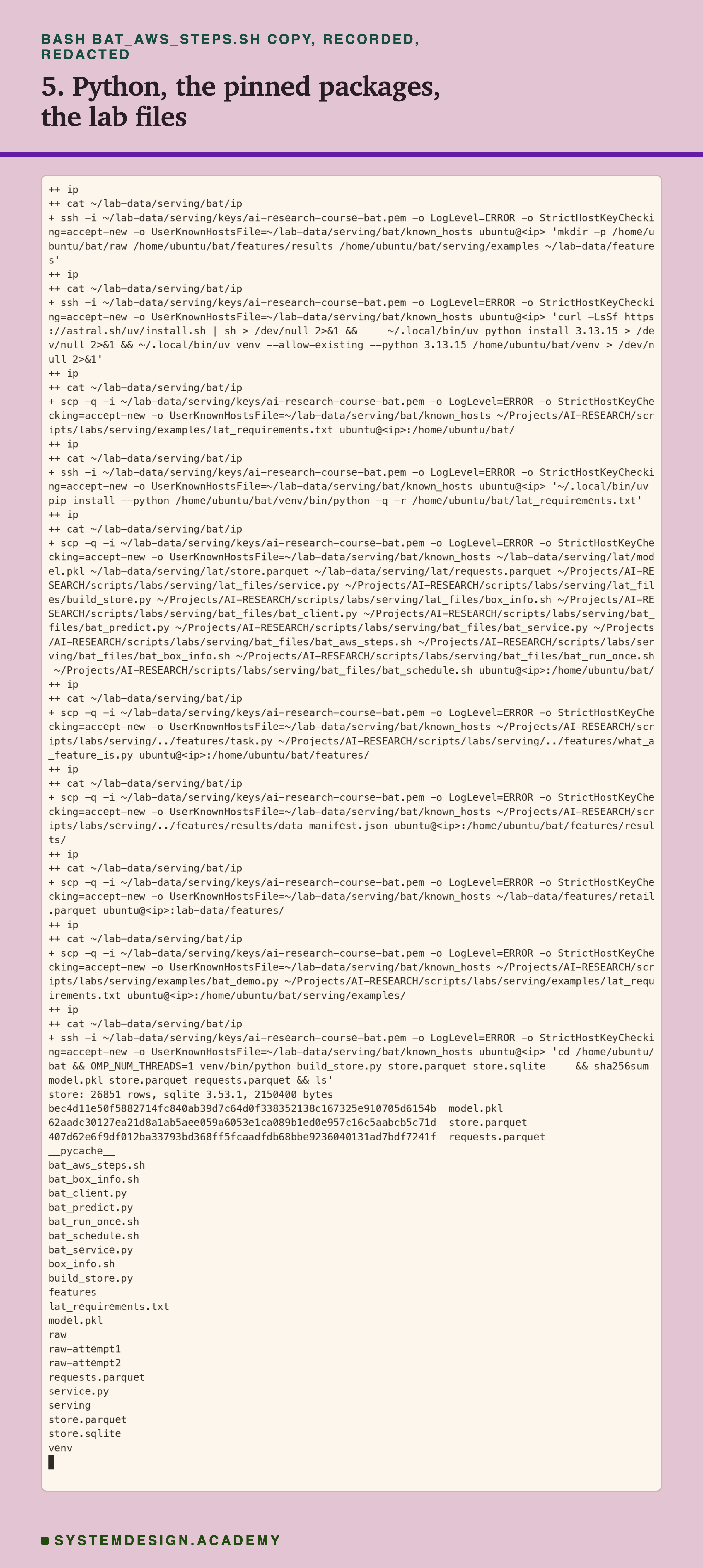
ssh "${SSH[@]}" ubuntu@"$IP" "mkdir -p bat/raw bat/features/results bat/serving/examples lab-data/features"
ssh "${SSH[@]}" ubuntu@"$IP" "curl -LsSf https://astral.sh/uv/install.sh | sh > /dev/null 2>&1 && \
  ~/.local/bin/uv python install 3.13.15 > /dev/null 2>&1 && \
  ~/.local/bin/uv venv --allow-existing --python 3.13.15 bat/venv > /dev/null 2>&1"
scp -q "${SSH[@]}" examples/lat_requirements.txt ubuntu@"$IP":bat/
ssh "${SSH[@]}" ubuntu@"$IP" "~/.local/bin/uv pip install --python bat/venv/bin/python -q -r bat/lat_requirements.txt"
scp -q "${SSH[@]}" ~/lab-data/serving/lat/model.pkl ~/lab-data/serving/lat/store.parquet \
  ~/lab-data/serving/lat/requests.parquet lat_files/service.py lat_files/build_store.py lat_files/box_info.sh \
  bat_files/bat_*.py bat_files/bat_*.sh ubuntu@"$IP":bat/
scp -q "${SSH[@]}" ../features/task.py ../features/what_a_feature_is.py ubuntu@"$IP":bat/features/
scp -q "${SSH[@]}" ../features/results/data-manifest.json ubuntu@"$IP":bat/features/results/
scp -q "${SSH[@]}" ~/lab-data/features/retail.parquet ubuntu@"$IP":lab-data/features/
scp -q "${SSH[@]}" examples/bat_demo.py examples/lat_requirements.txt ubuntu@"$IP":bat/serving/examples/
ssh "${SSH[@]}" ubuntu@"$IP" "cd bat && OMP_NUM_THREADS=1 venv/bin/python build_store.py store.parquet store.sqlite \
  && sha256sum model.pkl store.parquet requests.parquet && ls"

Step 8: watch without touching. While it runs, the schedule writes one progress line to the box's serial console after every run. The serial console is a log that AWS keeps for the box, and you can read it through AWS without logging in. So I could follow the runs and never disturb them.

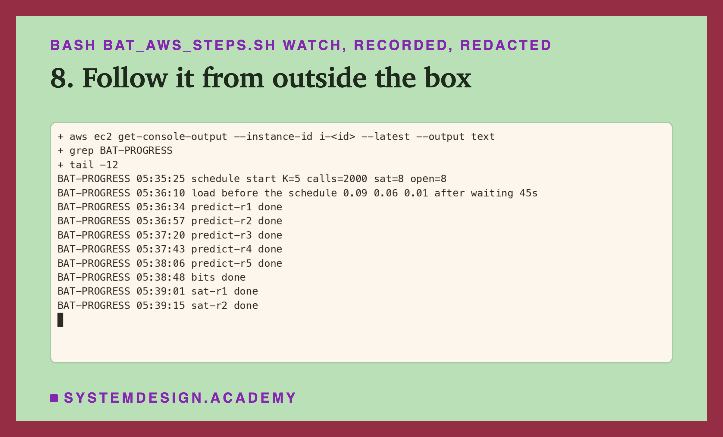
aws ec2 get-console-output --instance-id "$ID" --latest --output text | grep BAT-PROGRESS | tail -12

This recording comes from the first start of the schedule on this box, which later stopped working. The command is the same one I used to follow the run that produced the numbers. I explain the restart on the limits slide.

Step 11: the student demo, on the same box. After the schedule, I ran the demo you will meet later, so you can see what it prints on a quiet box. Its output went into a file at the same moment it went to the screen.

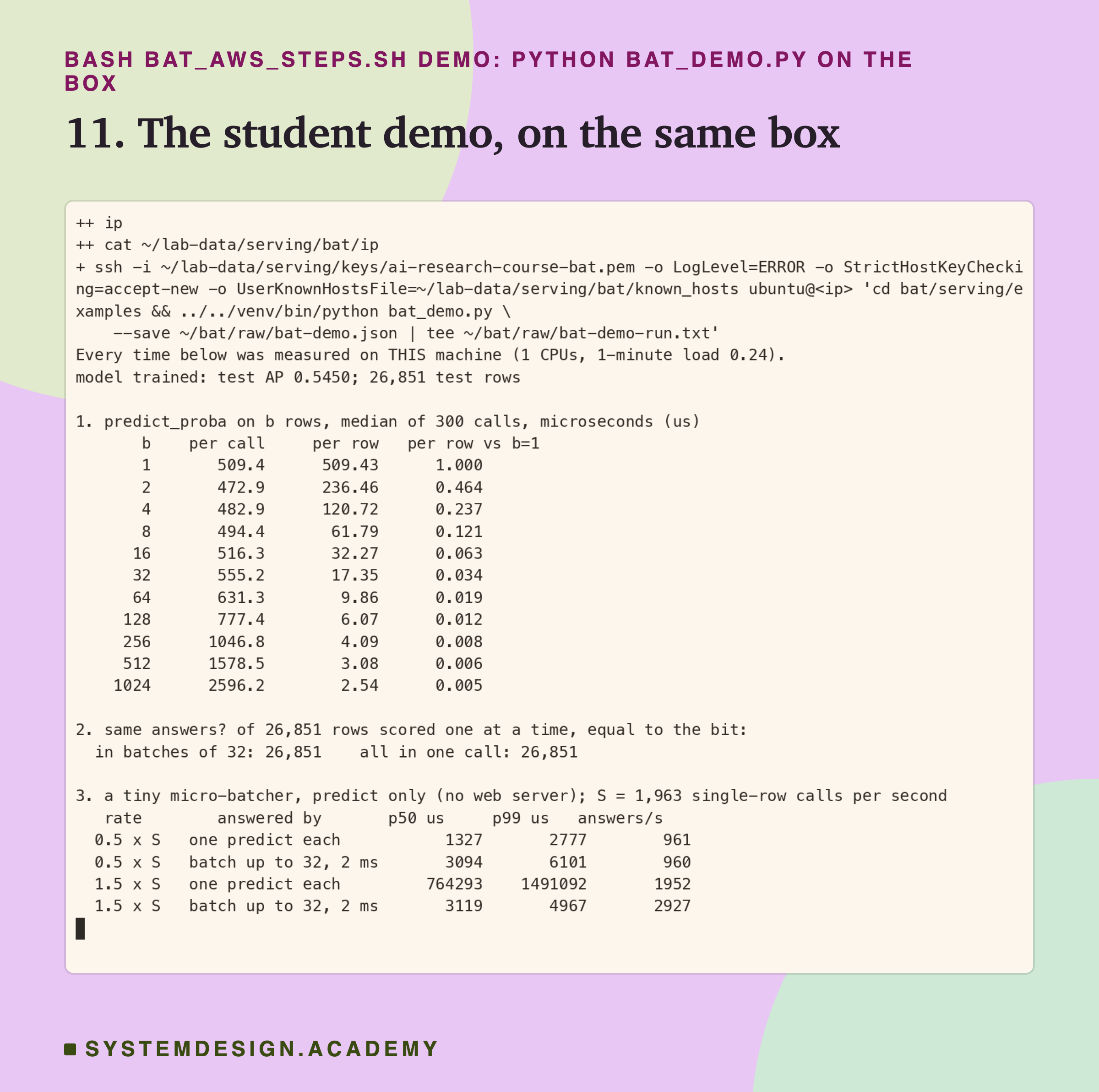
ssh "${SSH[@]}" ubuntu@"$IP" 'cd bat/serving/examples && ../../venv/bin/python bat_demo.py \
  --save ~/bat/raw/bat-demo.json | tee ~/bat/raw/bat-demo-run.txt'

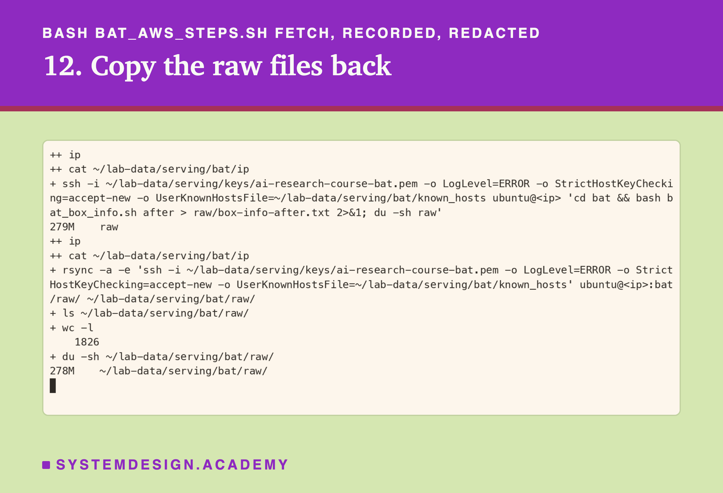
Step 12: bring the results home first. Lesson 3 lost a whole box of results because it was deleted before anyone copied them. So the rule is: the moment the runs finish, copy the raw files back, before anything else.

This is a real recording of the report script, bat_report.py. It ran on my laptop, but it times nothing. It reads the raw files the box measured and does all the arithmetic again with its own code.

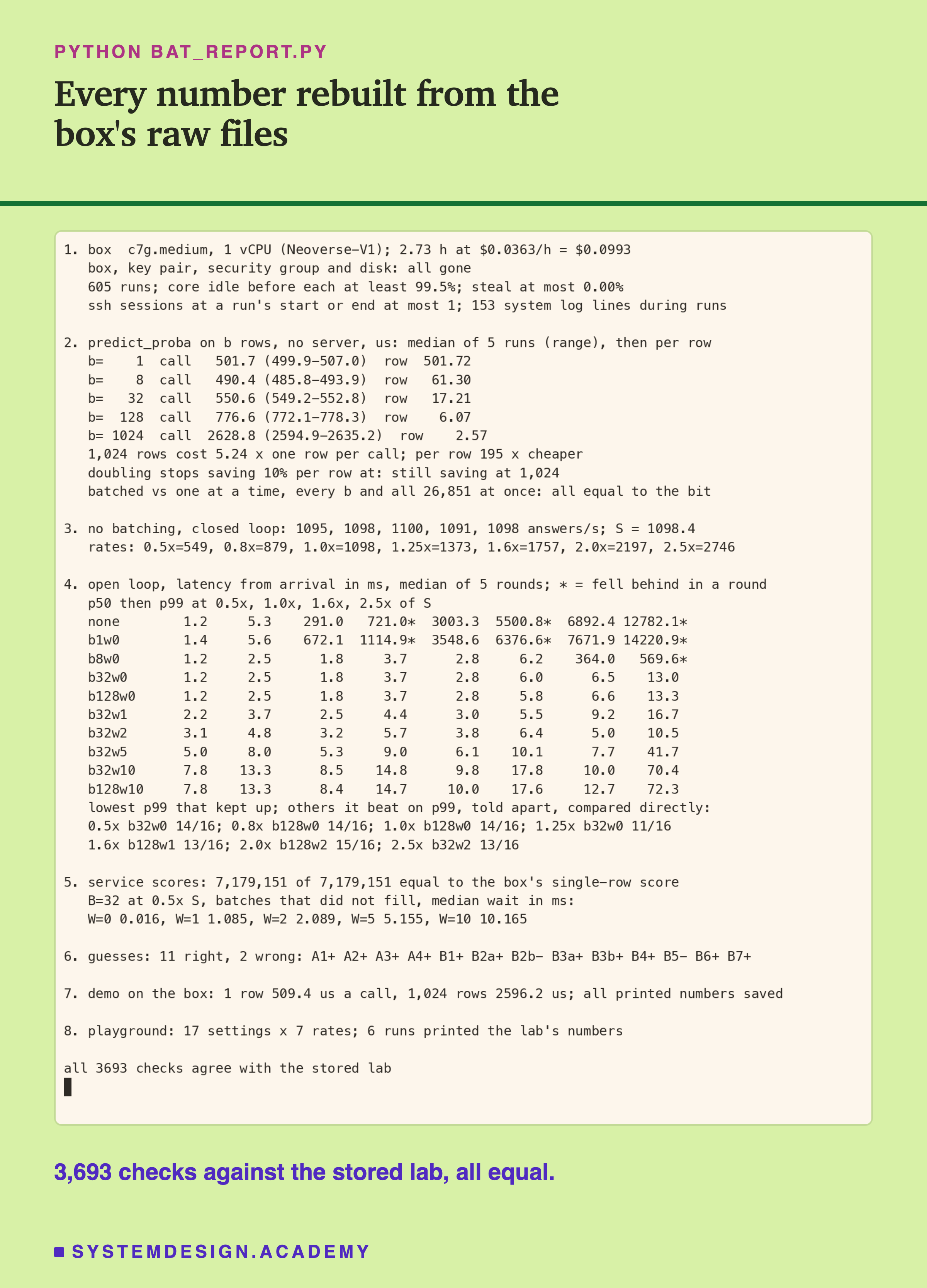
The report reads the small copy of the raw files kept in the repo. It computes its own percentiles, its own throughput, its own paired differences and its own verdicts. Then it compares every one with the lab's results file. If any number disagreed, it would stop with an error.

Section 1 is the quiet check. Before every one of the 605 runs, the core was at least 99.5% idle over two seconds, and the machine under my box took no measurable time from it. One SSH session was open at the start of the very first run of part A, the one that started the schedule as it logged out.

The system log had 153 lines during runs. Counted after the review: 86 came from the AWS management agent (SSM) in 5 runs, which tried to reach a web address and logged the error page it got back; 51 from cron, the older job scheduler, in 16 runs; 8 from sshd in 2 runs; 4 from the login manager in 2; 3 from systemd in 2; and 1 from the kernel.

I had stopped the systemd timers but not cron, so cron still ran.

First, the model alone, with no web server. How long does one call to predict_proba take on 1, 2, 4 and up to 1,024 rows?

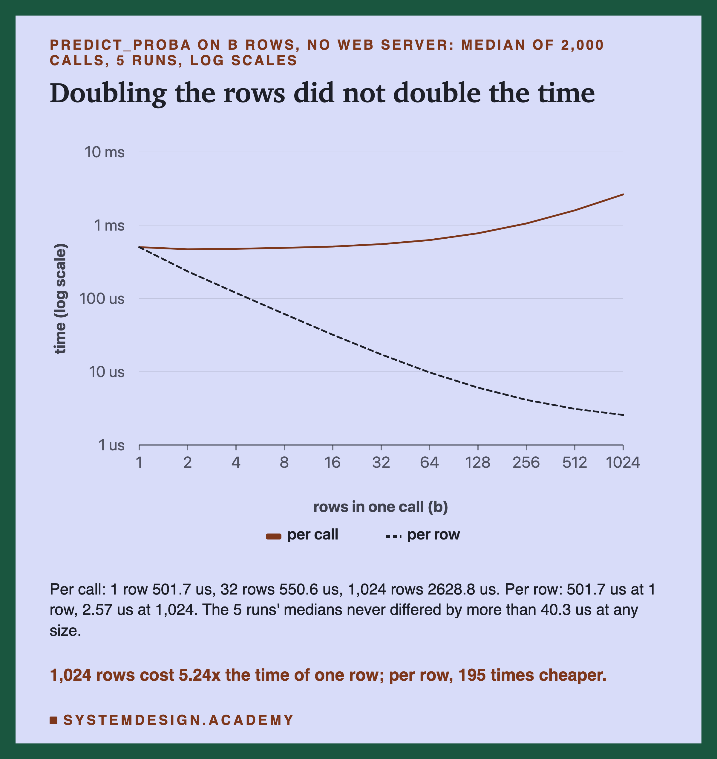
One row took 501.7 microseconds. 1,024 rows took 2,628.8 microseconds, only 5.24 times as long. So one row inside a batch of 1,024 cost 2.57 microseconds, 195 times less than one row alone.

The photocopier explains it. Most of a call's time is the walk to the machine: checking the input, setting up arrays, starting the model's code. That part costs about the same for 1 row or 100. The trees themselves are fast. The model has 54 trees, each with at most 31 leaves, and walking one row through all of them takes only a couple of microseconds.

Notice something odd at the left of the chart: 2 rows (468.9 us) and 4 rows (476.3 us) were faster per call than 1 row (501.7 us). I measured it in all five runs, but I did not find out why, so I only report it.

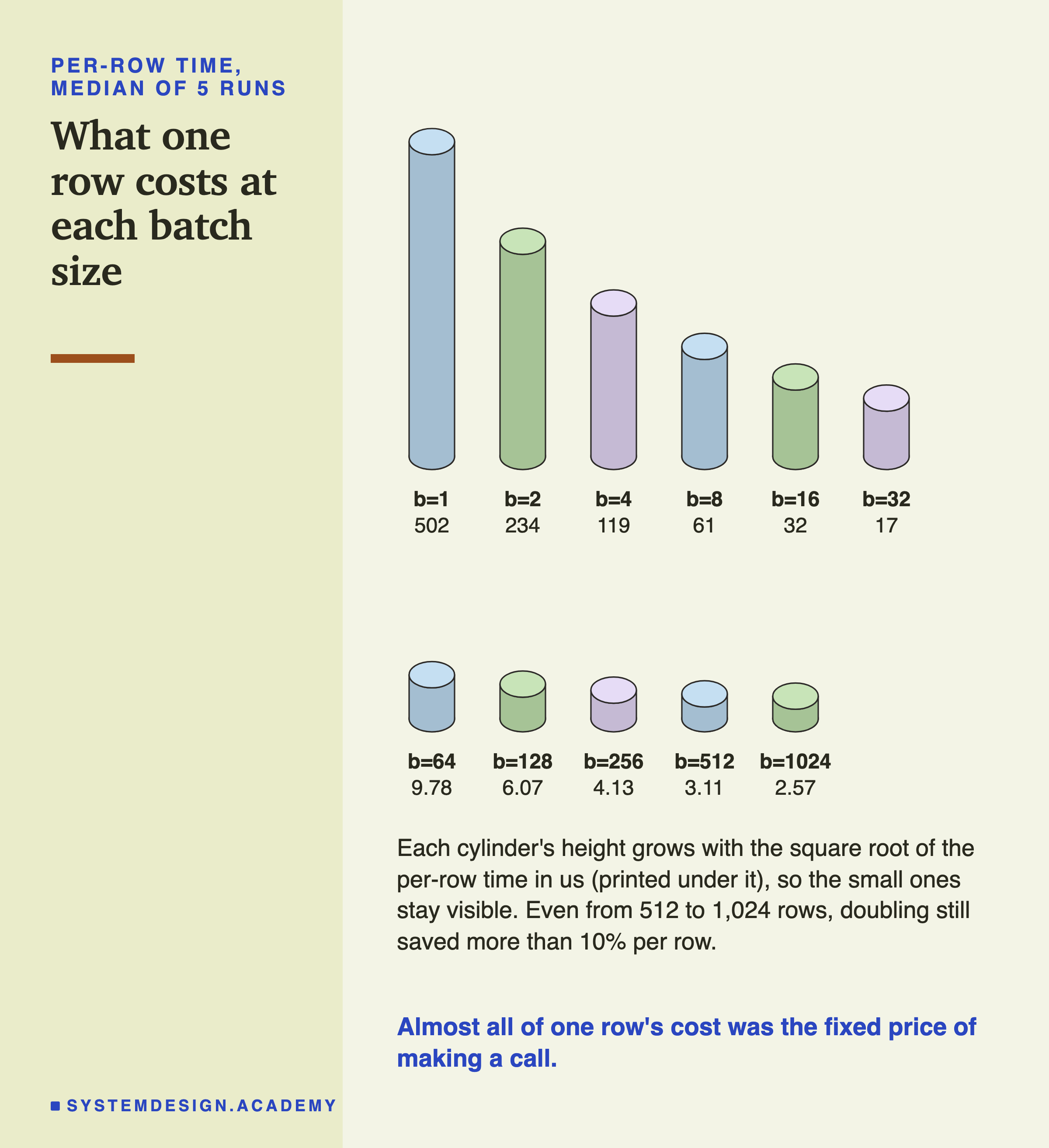
Where does the per-row cost stop falling? I fixed the rule before the runs: the first size at which doubling the batch saves less than 10% per row. It never happened. From 512 to 1,024 rows, the per-row time still fell from 3.11 to 2.57 microseconds, 17.5% less. So for this model, bigger batches kept getting cheaper per row all the way to the largest size I tried.

A batch is only useful if it gives the same answers. Does a row scored inside a batch get the same score as when it is scored alone?

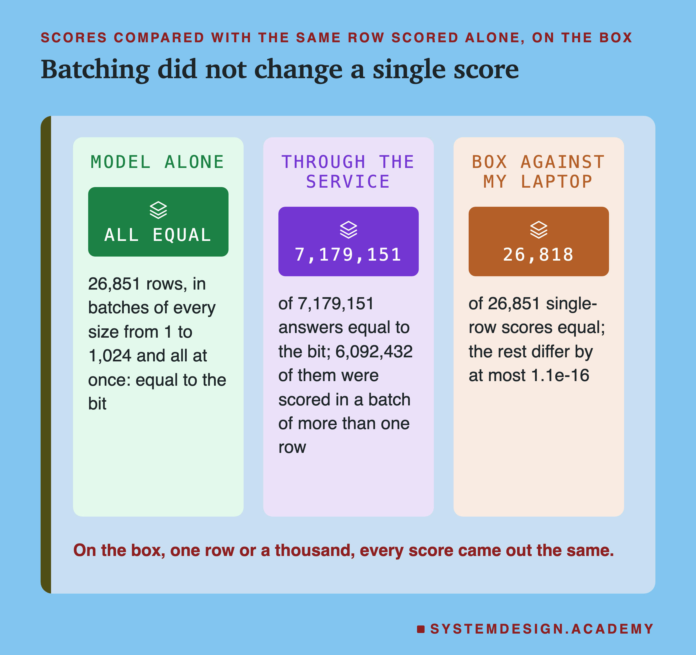
Yes, exactly. On the box I scored all 26,851 test rows one at a time. Then I scored them again in batches of every size from 2 to 1,024, and all 26,851 in one call. Every score was equal to the bit, which means every one of the 64 bits that store the number was the same. The tolerance was zero.

The service runs agree too. Every one of the 7,179,151 answers the service sent back, in all 595 open-loop runs, was equal to the bit to the box's own single-row score for that customer. That count includes the no-batching runs and batches of one row. Counted after the review, 6,092,432 of those answers were scored in a batch of more than one row.

The box and my laptop are a different story, and a familiar one from lesson 3. 26,818 of the 26,851 single-row scores matched my laptop's to the bit. The other 33 differed by at most 0.00000000000000011. Two different processors and builds of the same libraries can round the last bit differently. That has nothing to do with batching.

Before Part B, I needed one number: S, the most answers per second the service gives with no batching. Every arrival rate in Part B is a multiple of it.

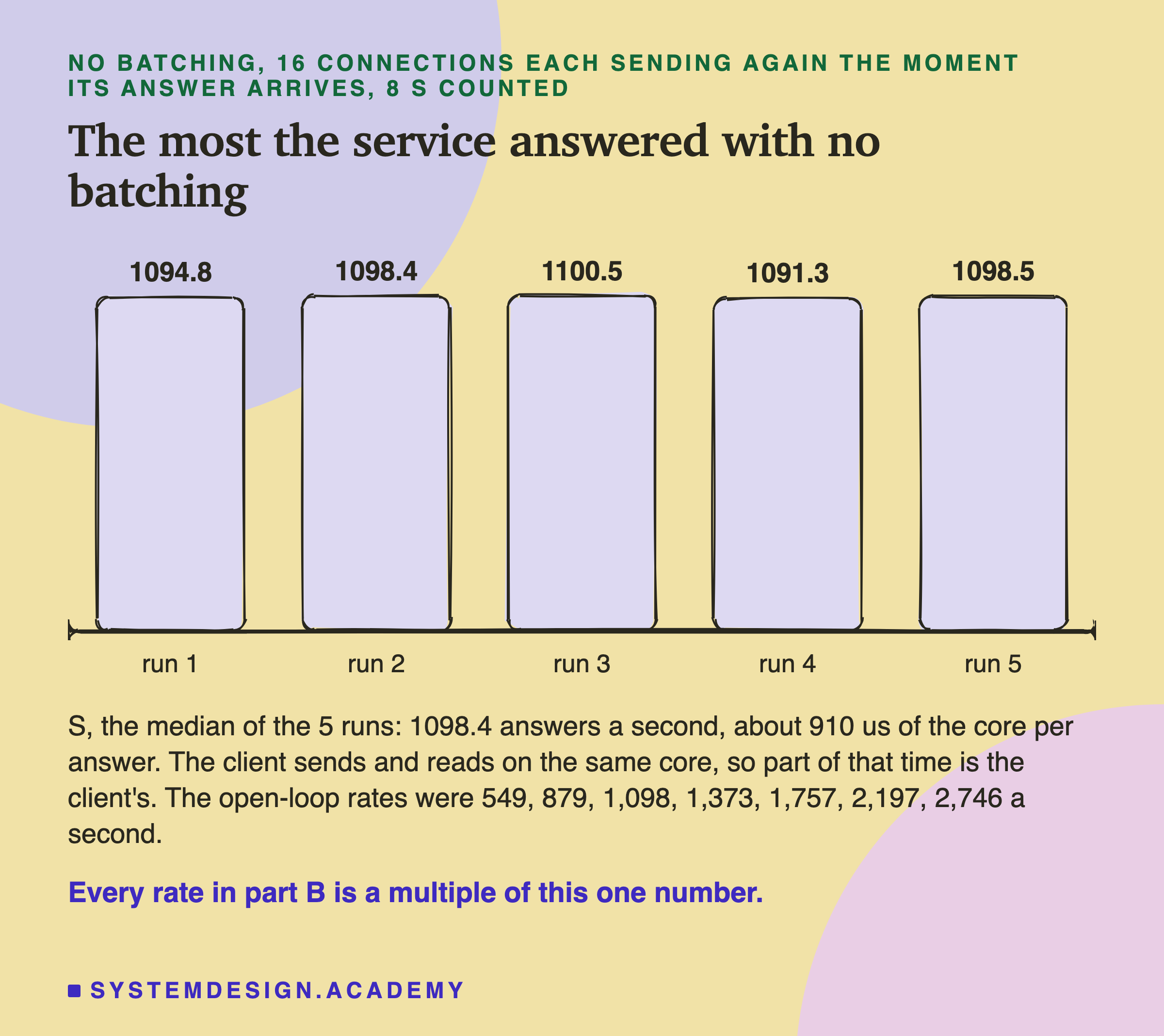
The five runs gave 1,091.3 to 1,100.5 answers a second, and S, their median, was 1,098.4. This works out to about 910 microseconds of the core for each answer, of which predict took 587 to 597 microseconds inside the service (its median at half and at 1.6 times S) and the rest is HTTP, checking the request, the SQLite lookup, the answer, and the client.

So the seven rates in Part B were 549, 879, 1,098, 1,373, 1,757, 2,197 and 2,746 requests a second.

One thing S does not tell you. S came from a closed-loop client, which is cheap to run. The open-loop client in Part B uses two threads and a pool of 512 kept-alive connections, connections that stay open between requests instead of being made fresh for each one, and it spends more of the shared core on each request. With that client, no batching could only give about 1,034 to 1,045 answers a second, a little below S.

This is most likely why no batching already fell behind at exactly S. I did not test it. Another possible reason is the 512 connections themselves: the service has to watch many more open connections than the 16 of the saturation runs.

Here is what one batch does, using a real example: B = 32, W = 2 ms, at half of S, 549 requests a second.

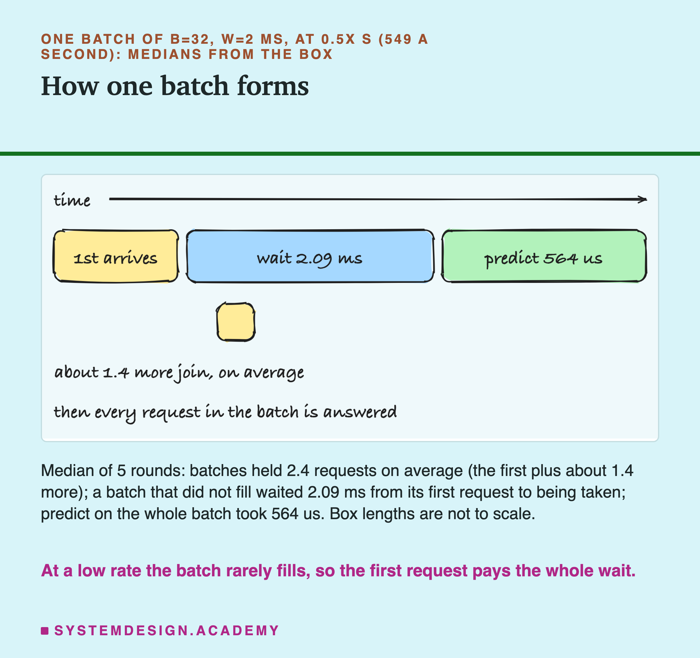
Each request first goes through the same steps as in lesson 2: read the body, check it, look up the six features in SQLite. Then, instead of calling the model, the handler puts its row in a list and waits. One batcher task, a small loop running inside the same server, watches the list.

When the first row arrives, the batcher starts a timer for W. If B rows arrive before the timer ends, it takes them at once. If not, it takes whatever is there when the timer ends. Then it calls predict_proba once for the whole batch, and hands each request its own score.

At 549 requests a second, about one request arrives every 1.8 ms. So in a 2 ms wait, only one or two more come. These batches held 2.4 requests on average, never close to 32. The first request in each batch waited about 2 ms for almost nothing.

With W = 0, the batcher does not start a timer. It takes whatever rows have gathered by the time it gets to run. At half of S those batches held only 1.2 requests on average. But, as the next slide shows, those few small batches still mattered.

At half of S, the service with no batching keeps up easily. So what does a batcher do there? For each setting, I subtracted the no-batching median latency from the setting's median latency, in the same round, on the same arrivals.

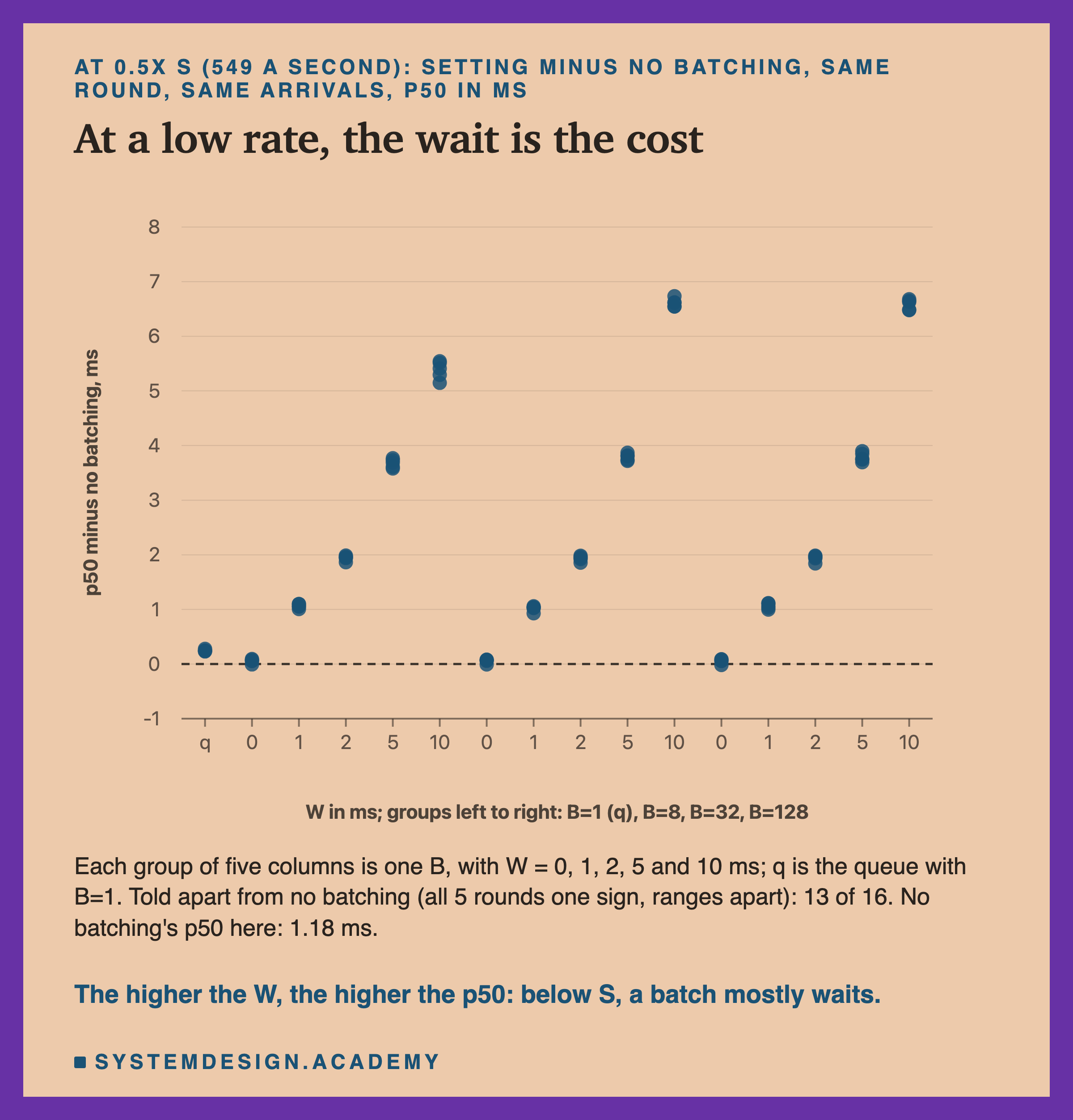
Every timed wait raised the median. No batching had a p50 of 1.18 ms. With B = 32, W = 1 gave 2.20 ms, W = 2 gave 3.11, W = 5 gave 4.99 and W = 10 gave 7.80. All twelve settings with a W of 1 ms or more had a higher p50 than no batching, told apart in all five rounds. The cost was roughly the wait itself, because at this rate batches rarely fill.

W = 0 cost almost nothing at the median. For B = 8, 32 and 128 with W = 0, the p50 was 1.24 ms against 1.18 ms, and that difference cannot be told apart from run-to-run noise. In round 4, all three went the other way, by 6, 8 and 18 microseconds.

But W = 0 cut the p99 in half. At the same rate, no batching had a p99 of 5.26 ms, and B = 32 with W = 0 had 2.50 ms. All five rounds agreed, by 2.4 to 3.3 ms.

Why would batching help when the service is only half busy? Random arrivals come in clumps. Sometimes four requests arrive within a millisecond. With no batching, they are scored one after another, about 0.9 ms each, so the fourth waits behind three others. With W = 0, the requests that gathered while the model was busy are scored together in one call, for about the price of one. The clump clears quickly, so the slowest requests are not so slow. The median request rarely meets a clump, so the median barely moved.

I checked the clump idea after the review, so it is a labelled addition. With no batching at half of S, the slowest 1% of requests had 4.5 to 4.9 arrivals in the 3 ms before them, against 1.60 to 1.69 for all requests, in all five rounds. So the slowest requests did arrive in clumps. That fits the explanation, but it does not prove that scoring the clump together is what helped.

Did a batch with W = 1 ms really wait 1 ms? I measured, for every batch that did not fill, the time from its first request joining the list to the batcher taking the rows.

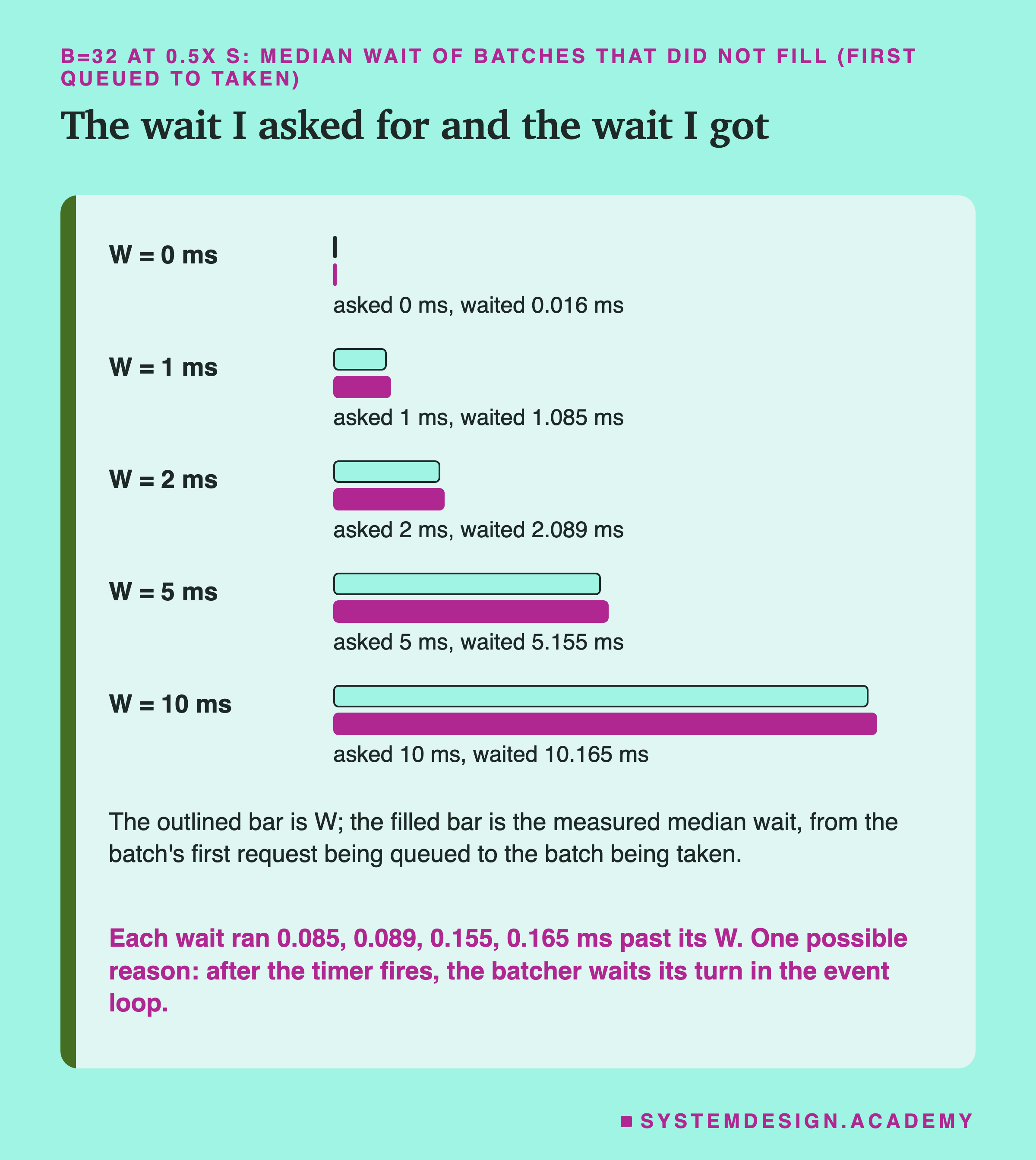
Each wait ran a little longer than asked: 1.085 ms for W = 1, 2.089 for W = 2, 5.155 for W = 5 and 10.165 for W = 10. With W = 0 there was no timer, and the median wait was 16 microseconds.

The batcher runs inside the service's event loop, the part of the server that switches between all its waiting jobs on one thread. The batcher's timer uses loop.call_later. Python's documentation describes it as "Schedule callback to be called after the given delay number of seconds". The service runs on uvloop, a faster event loop for Python, which is built on a library called libuv, and libuv's documentation says its timers' "timeout and repeat are in milliseconds".

So I guessed, before the runs, that a 1 ms wait would come out somewhere between 1 and 2 ms, and it did. The extra was 85 to 165 microseconds, not a whole millisecond. One possible reason for the extra is that after the timer fires, the batcher still waits its turn among the other tasks in the event loop. I did not test that.

The lesson for a real service: the W you set is a floor, not an exact time.

Now the busy side. This chart follows the median latency of five settings as the arrival rate rises.

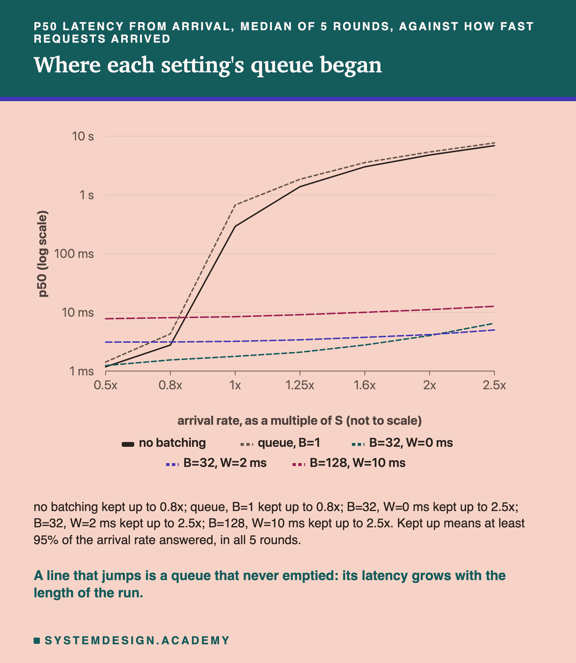
No batching kept up to 0.8 times S and no further. At 0.8x its p50 was 2.77 ms and its p99 16.4 ms. At 1x the p50 jumped to 291 ms, and at 2.5x to 6.9 seconds. The queue with B = 1 broke at the same place, and was worse at every busy rate.

Every setting with B of 32 or 128 kept up at every rate, in all five rounds. So did B = 8, except at 2.5 times S, where it kept up in only 2 of 5 rounds. A cap of 8 rows per call was too small for that rate: even in the two rounds that kept up, its p50 was about 310 and 360 ms, because up to 5% of a run's requests may pile up and still count as keeping up.

Look at the numbers above S with care. A setting that does not keep up has a queue that grows for the whole run. If my runs had lasted 16 seconds instead of 8, its latencies would have been larger still. So for no batching above S, "721 ms" really means "the queue never emptied". It is not a stable number.

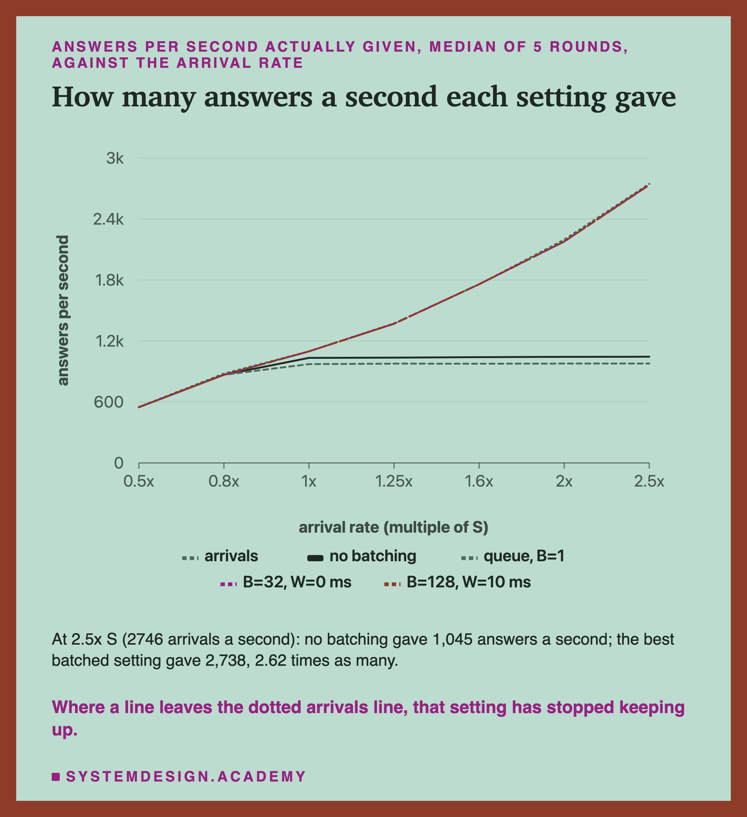
Throughput tells the same story in answers per second. No batching topped out at about 1,034 to 1,045 answers a second. The queue with B = 1 topped out lower, at about 972 to 978. The best batched settings gave 2,738 answers a second at 2.5 times S, at least what no batching gave. Batching's own limit was not reached: I stopped at 2.5 times S, so I do not know where batching itself would have run out of room.

Which batched setting was best? Here is every one of them at 1.6 times S, 1,757 requests a second.

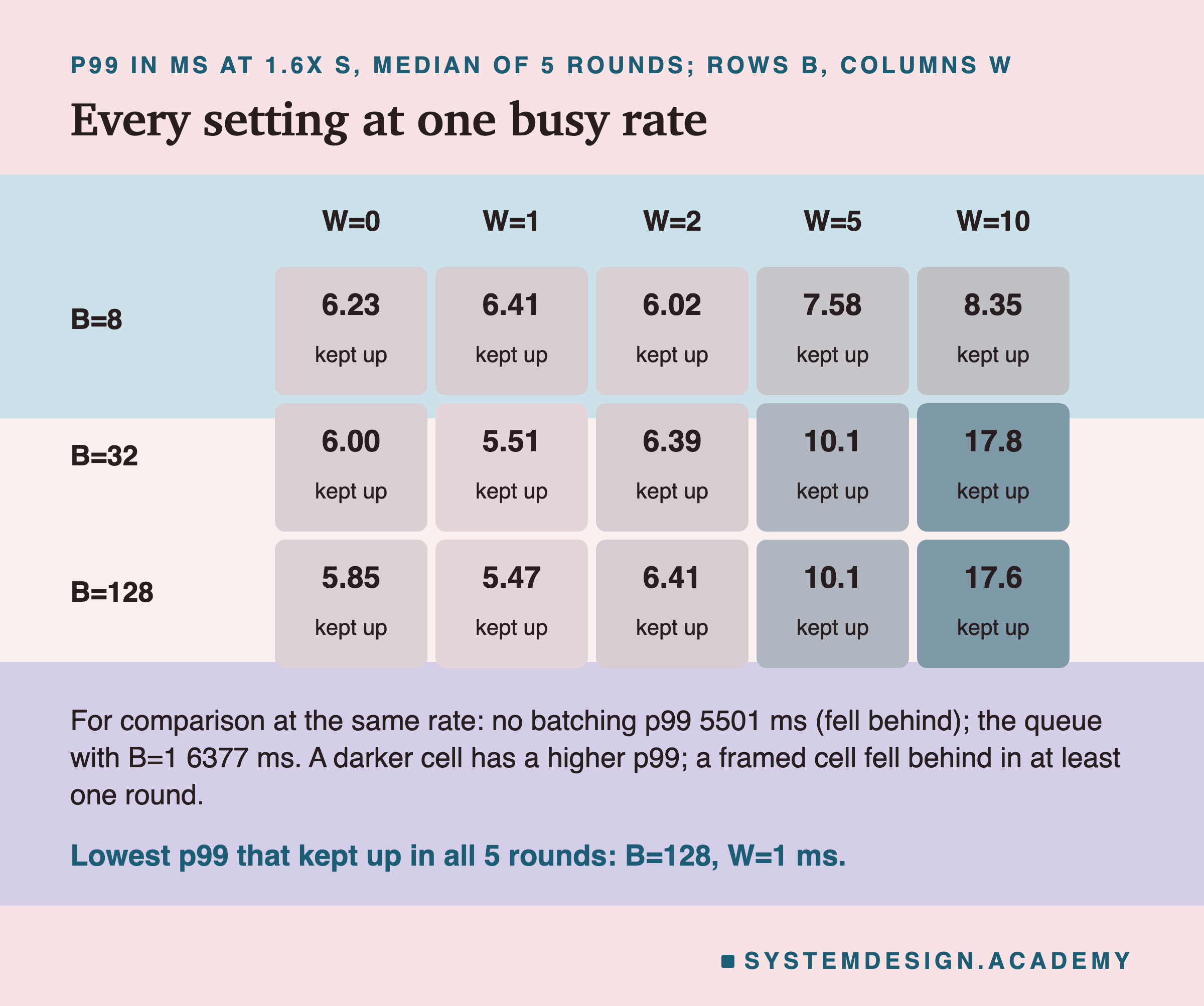
At this rate, every batched setting kept up, and the p99s ran from 5.47 ms to 17.8 ms. No batching was at 5,501 ms. Next to that gap, the differences between batched settings are small.

The lowest p99 was B = 128, W = 1 ms, at 5.47 ms. But compared directly, round by round, it could not be told apart from B = 32 with W = 0 or 1, or from B = 128 with W = 0. So I cannot say it was better than those three.

The large waits were clearly worse. With W = 10 ms the p99 was about 17.6 to 17.8 ms. And at 2 and 2.5 times S, W = 10 got much worse: B = 32, W = 10 had a p99 of 50.1 ms at 2 times S and 70.4 ms at 2.5 times S, against 8.18 ms and 13.0 ms for W = 0. I did not find out what made the long waits so much worse at those rates.

When did a timed wait beat no timed wait? After seeing the results, I checked each setting with a W of 1 ms or more directly against all three W = 0 settings with a cap of 8 or more. This check was not in the design, so I label it as added later.

A timed wait had a lower p99 than all three, told apart, only twice: B = 32 with W = 1 at 1.6 times S, and B = 32 or 128 with W = 2 at 2 times S. At 2.5 times S, the setting with the lowest p99, B = 32 with W = 2 at 10.5 ms, could not be told apart from B = 32 or 128 with W = 0, or from B = 128 with W = 2.

So on this box, a timed wait sometimes helped a little at high rates, and cost a lot at low rates. W = 0 with a cap of 32 or 128 was never far from the best, at any rate.

The service also recorded three moments for every request: when the handler started, when the row was ready for the model, and when the score came back. For four of the runs, the repo keeps those readings.

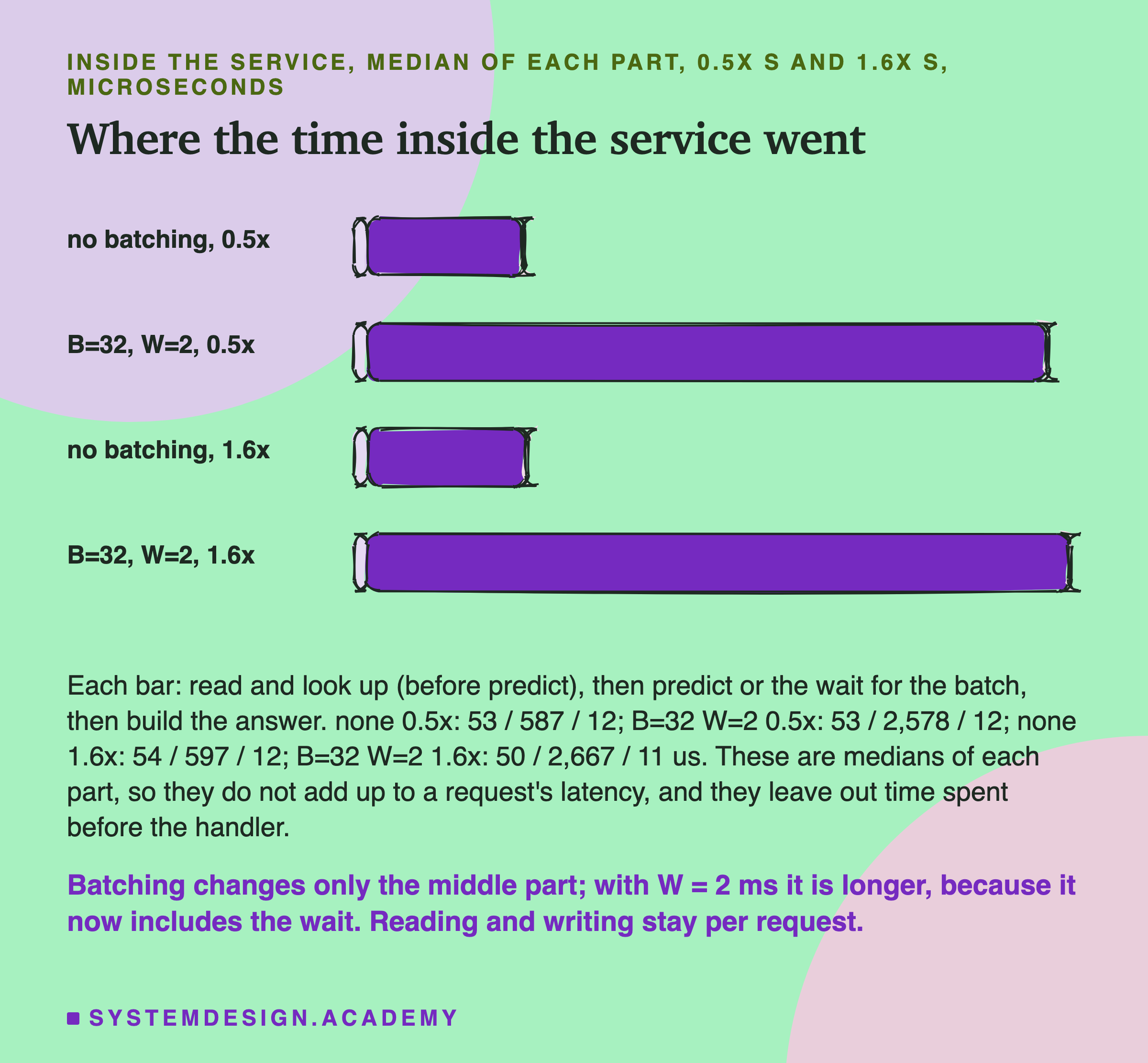
Inside the handler, reading the body, checking it and the SQLite lookup took a median of about 50 microseconds, and building the answer about 12. With no batching, the middle part, the model call itself, took about 590 microseconds. With B = 32 and W = 2, the middle part was the wait for the batch plus the batch's model call: about 2,600 microseconds.

The handler's own work is small. But the whole core spends about 910 microseconds per answer at S, so most of a request's cost is outside the handler: the web server reading and writing HTTP, and the client. Batching does nothing about that part. So the batched service's throughput, though 2.62 times higher, is not 195 times higher like the model's per-row cost.

Everything above is one small tree model on one CPU core. I did not measure any other machine, so I give no numbers for one. But the measurements here show which parts of the answer would change, and why.

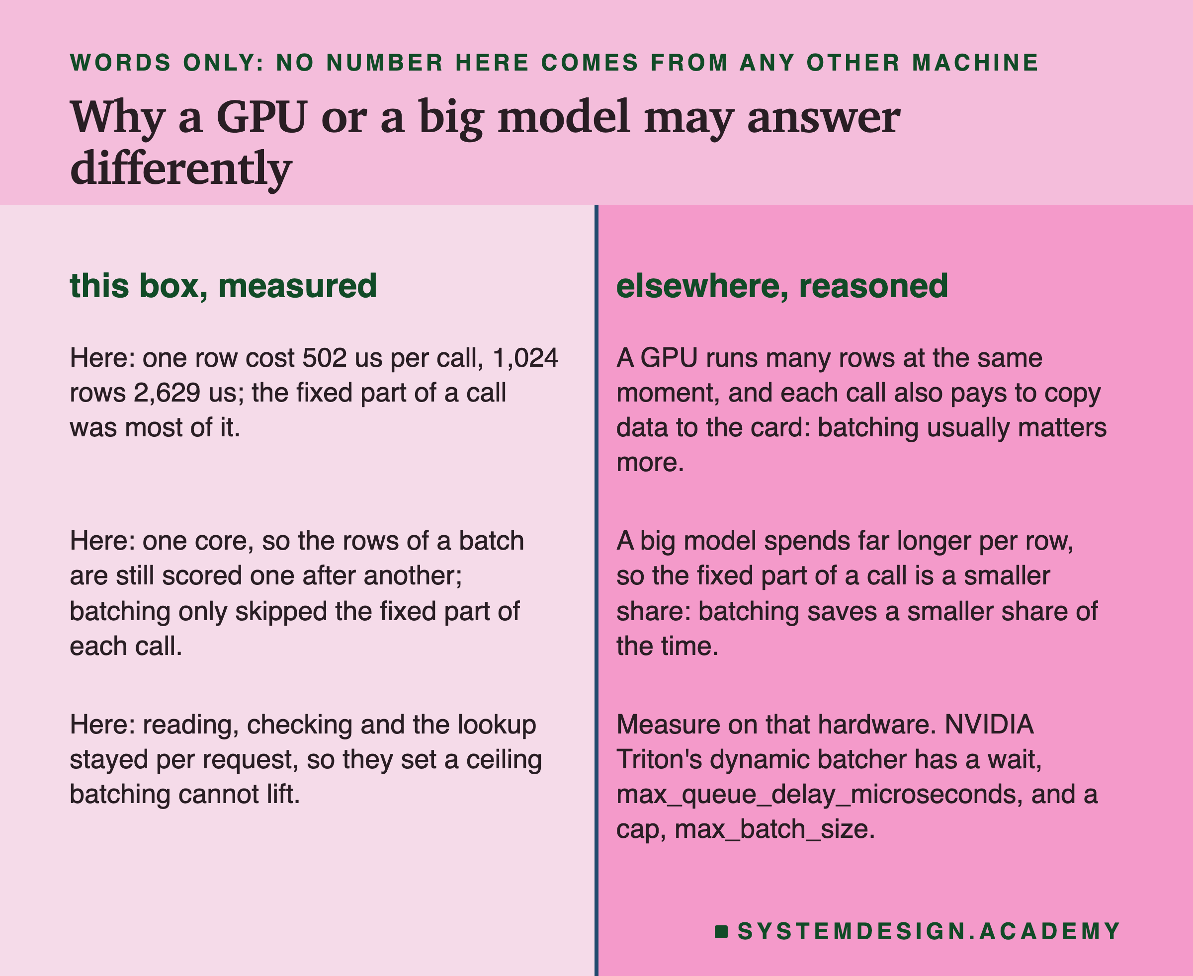
What batching saved here was the fixed cost of a call. On one core, the rows of a batch are still scored one after another, and each row still costs its couple of microseconds. Batching only stopped me paying the 500-microsecond walk to the photocopier for every row.

A GPU changes the per-row part. A GPU is a chip that does thousands of small calculations at the same moment. Many rows can be scored at once, not one after another, so a bigger batch can cost almost the same as a small one even when the model is large. Each call also has to send its data to the GPU's own memory and back, another fixed cost. Both of those make batching matter more on a GPU, which is why serving systems for GPUs usually batch.

A big model changes the balance. If one row took 10 milliseconds of real work, the fixed 500 microseconds would be a small share of it. Batching would save a smaller share of the time on a CPU, and the extra latency of a timed wait would be smaller compared with the work.

These are reasons, not measurements. If you serve on other hardware, measure Part A on it first. Batching servers built for GPUs expose the same dials I used. For example, NVIDIA's Triton Inference Server documents a dynamic batcher with a max_queue_delay_microseconds setting, like my W, and a max_batch_size setting, the largest batch, like my B. Its setting is a preference for certain sizes, not a cap.

I wrote eleven guesses into the lab before it ran. Two of them had two parts, so the report checks thirteen statements. Eleven were right and two were wrong.

1. "predict on 1 row: median per call between 450 and 700 us." Right: 501.7 us.

2. "1,024 rows cost less than 10 x the time of 1 row per call." Right: 5.24 times.

3. "Per-row cost still falling by 10% or more from 512 to 1,024." Right: it fell by 17.5%.

4. "Every batched score equals the single-row score to the bit, for every b." Right.

5. "S between 800 and 1,300 answers per second." Right: 1,098.4.

6. "At 0.5 x S, every setting with W at least 1 ms has a higher p50 than none, told apart; every W = 0 setting's p50 cannot be told apart from none's." First part right: 12 of 12. Second part wrong: the queue with B = 1 had a p50 244 us higher, told apart. The three W = 0 settings with a real cap could not be told apart from no batching.

7. "At 1.25 x S and above, none does not keep up; b32w2 keeps up at 1.6 x S and 2.0 x S, with a lower p99 than none, told apart." Both parts right. No batching kept up in 0 of 5 rounds at every one of those rates.

8. "The highest throughput of any setting at 2.5 x S is at least 1.5 x none's." Right: 2.62 times.

9. "b1w0 has a p50 within 50 us of none's at 0.5 x S." Wrong: 244 us. The batcher's machinery costs more than I thought.

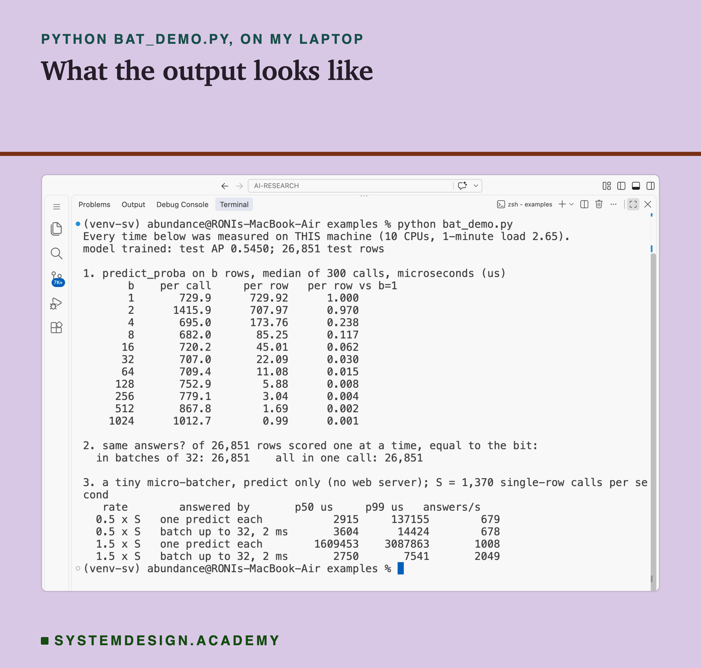
The full lab needs a rented box and about two and a half hours. The demo, bat_demo.py, runs on your own computer. It times the model on batches, checks the scores, and runs a tiny batcher with no web server.

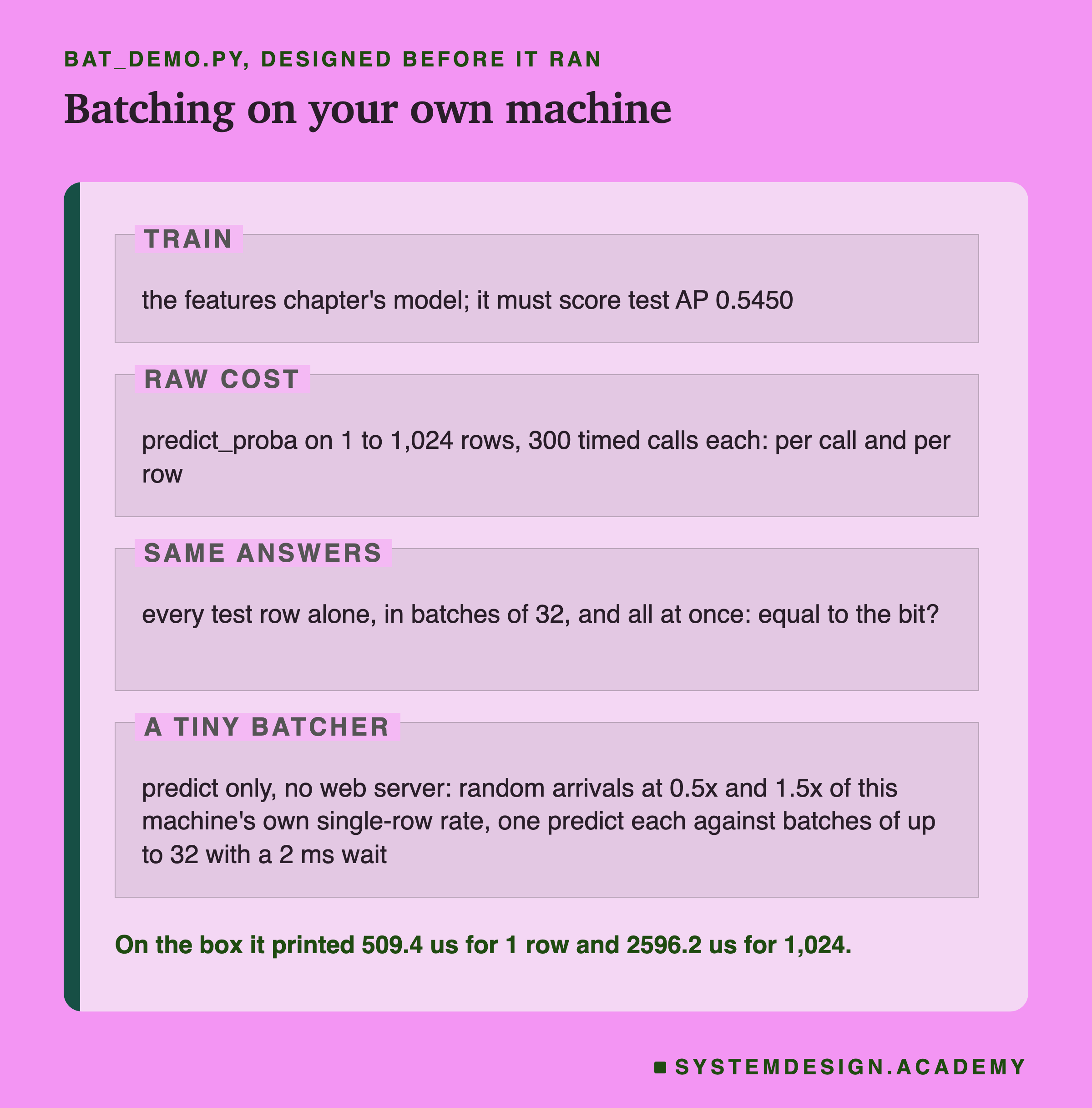
I wrote the demo's design into its docstring after the lab's design and before the demo first ran. I did not change it after the results.

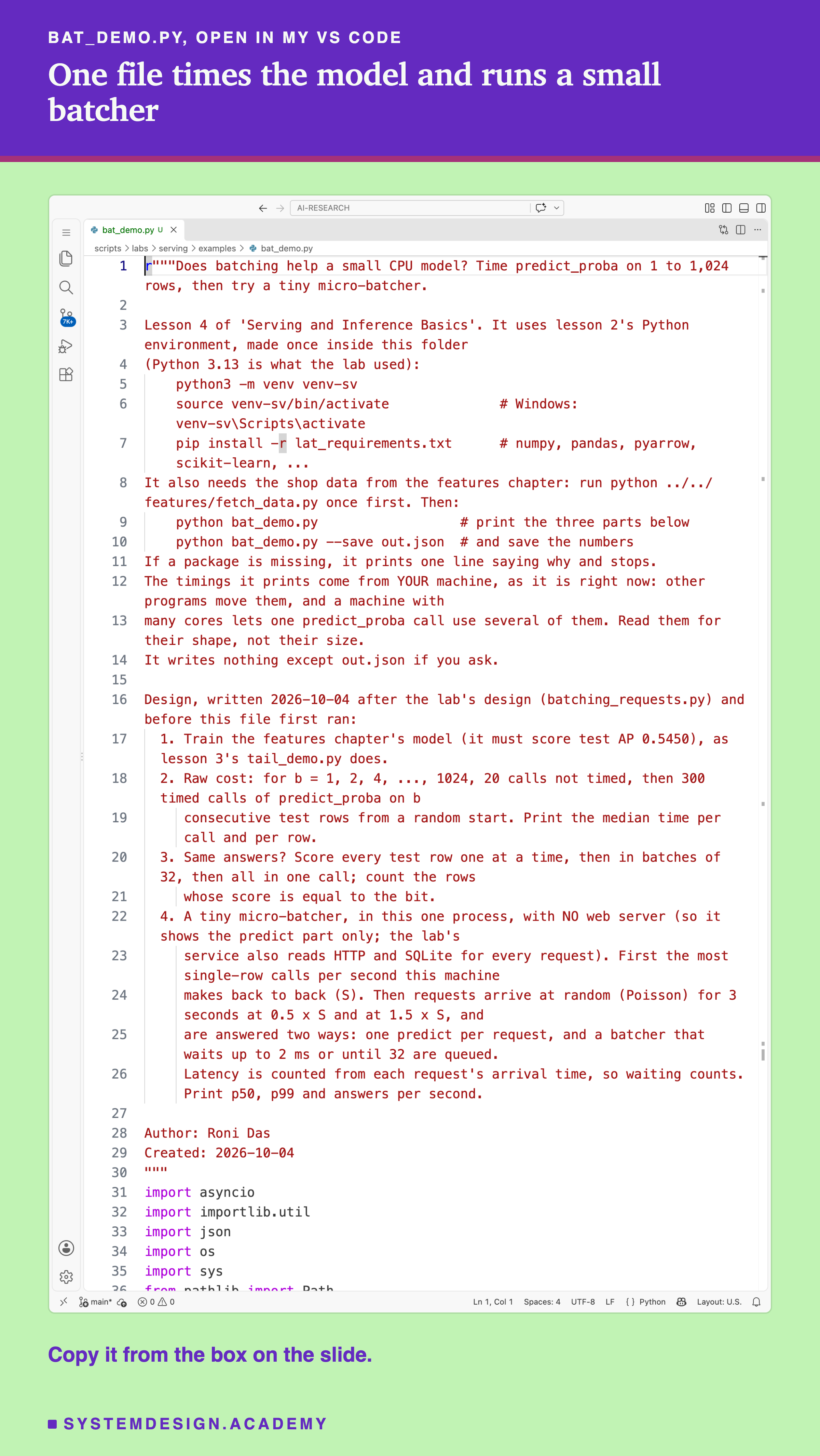
Before you run this lab. The demo uses lesson 2's Python environment, with the same library versions as the lab's box. If you made it for lesson 2 or 3, use it again. If not, make it once, inside the scripts/labs/serving/examples folder:

python3 -m venv venv-sv
source venv-sv/bin/activate        # on Windows: venv-sv\Scripts\activate
pip install -r lat_requirements.txt

I used Python 3.13. Then run python ../../features/fetch_data.py once, which downloads the shop data. Now run python bat_demo.py. It needs no GPU, no web server and no cloud account. If a package is missing, it prints one line saying why and stops.

The first line it prints says the times are from your machine, with its number of CPUs and its load at that moment. Read them for their shape, not their size. On a machine with many cores, predict_proba may use several of them in one call, so the per-call times can look quite different. Does the per-row cost fall as the batch grows? Are the batched scores the same? Does the tiny batcher keep up where one predict each falls behind?

This box holds the real results from the lab. It needs nothing but Python, so it runs in your browser. It has no model and no clock: it only looks up what the box measured.

Press Run. Then try B = 1 to see the queue with batches of one. Try W = 10 at RATE = 0.5, then at RATE = 2.5. Try B = 8, W = 0 at RATE = 2.5, where a cap of 8 was too small.

The report script writes this box from the lab's raw files, runs it with six settings, and checks that each run prints the lab's numbers. Every line shows no batching first, at the same rate, so you always compare with it.

The lab has one file that runs on my laptop, a few small files that run on the box, and the step script you saw above.

batching_requests.py, on my laptop, holds the design in its docstring, written before the first timed run, with dated notes added later. Its commands are check (lesson 2's files match by sha256), status (reads the box's serial console), collect, cost and factcheck. collect calls bat_stats.py, which makes a small copy of the raw files in results/bat-raw/ and does all the arithmetic on it.

bat_files/bat_predict.py is Part A. It loads the model and the 26,851 real test rows and times predict_proba on 1 to 1,024 rows. Its bits command scores every row alone and in batches and compares the scores bit by bit.

bat_files/bat_service.py is the service. It imports lesson 2's service file unchanged, so the model, the SQLite table and the request checks are lesson 2's. With no batching, the handler calls predict_proba on its one row, as in lesson 2. With batching, the handler puts its row and a in a list and waits. A future is an empty box for an answer: the handler waits on it, and someone else fills it in later. The batcher task takes up to B rows off the list, calls once, and fills in every future.

Here is the order I would follow, using only what this lab did.

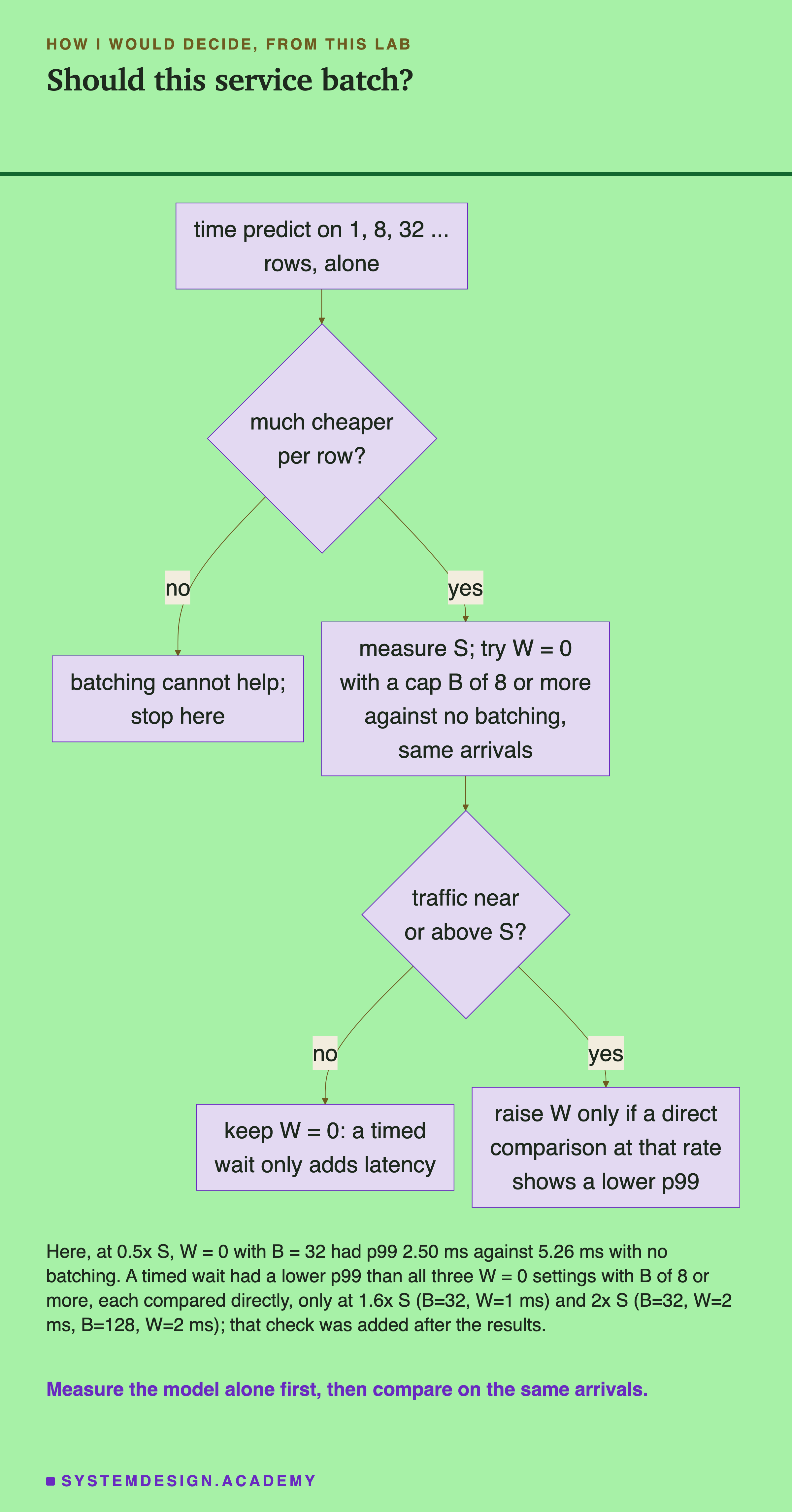
The chart starts with the cheapest test, the model alone, and only then brings in the service and its traffic. Here are the same steps in words, each with the number from this lab behind it.

1. Time the model alone first. Call it on 1, 8, 32 and more rows. If one row in a batch is not much cheaper than one row alone, no batcher can help, and you can stop. Here it was 195 times cheaper at 1,024 rows.

2. Measure S, with no batching. It tells you where the service will fall behind. Here no batching fell behind at S and gave at most about 1,045 answers a second.

3. Test with random arrivals, and count from arrival. A test that waits for each answer before sending the next can never show a queue. Lesson 7 of this chapter measures what that kind of test hides.

4. Start with W = 0 and a cap. Here it never did worse than no batching on p99, and from 0.8 times S up it was better on p50 too.

5. Compare settings on the same arrivals, directly. Two settings that each differ from no batching are not ranked by that. Compare them with each other.

Batching helps when the fixed cost of a call is large compared with the cost of a row. Here the fixed part was about 500 microseconds and a row about 2.6, so batching saved almost everything the model spent.

It helps most when traffic comes near or above S. Here, no batching fell behind at S. Batches of up to 32 or 128 kept up at 2.5 times S.

It can help a little even when the service is quiet, if it does not wait on purpose. At half of S, W = 0 halved the p99 by scoring the clumps of random arrivals together.

A timed wait is a cost at low traffic. Every W of 1 ms or more raised the median at half of S, by about the length of the wait. If your traffic is quiet most of the day and busy for an hour, a fixed W makes every quiet request slower to help the busy hour.

A batcher that never groups requests is pure cost. The queue with B = 1 had a higher p50 than no batching at every rate, and once both fell behind it gave fewer answers a second.

Do not batch blindly into a model you have not checked. Batching changed no score here, to the bit. Check yours the same way before you trust it.

Do not copy my handler as it is into a busy service. Like lesson 2's, it is an async def that calls SQLite and predict_proba, which block the event loop while they run. On one core with one worker, that is what I measured on purpose. With more cores, lesson 5 measures workers and threads.

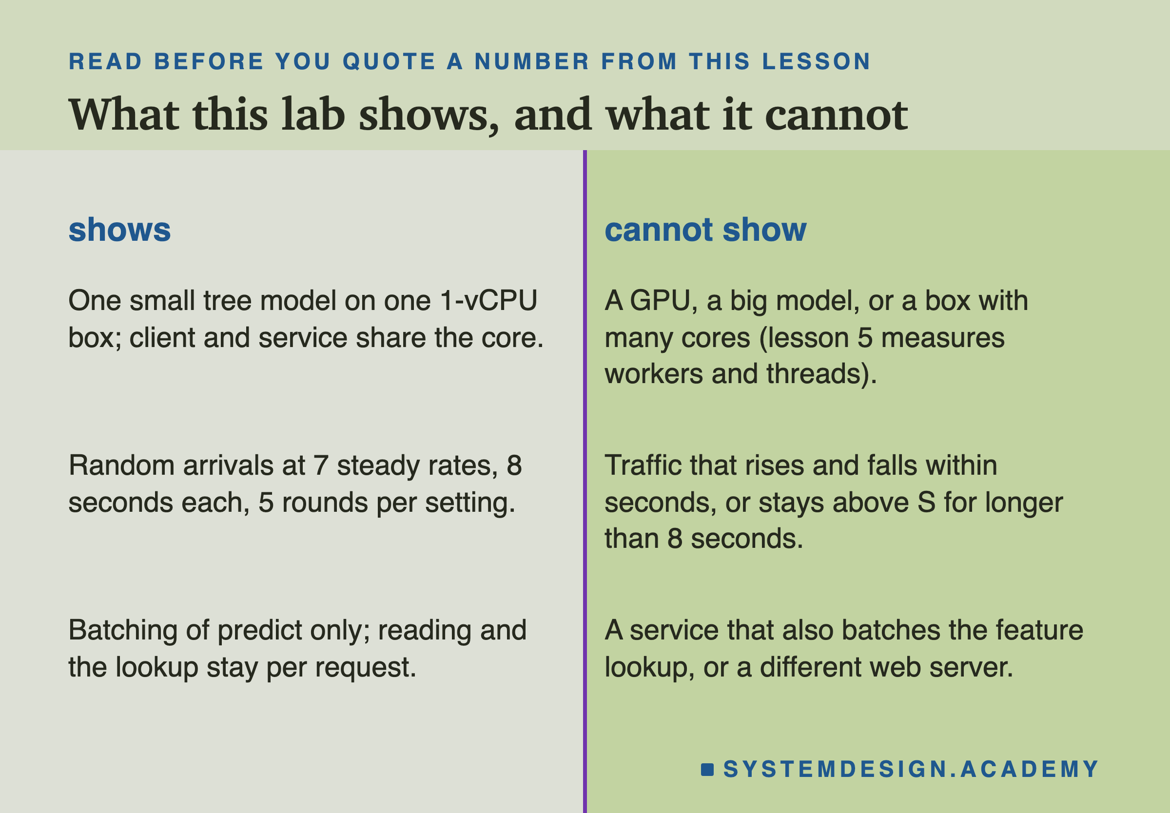
One small model, one core, one shared client. The client took part of the core in every run. A service with its client on another machine would answer more per second, with or without batching.

Steady rates for 8 seconds. Real traffic rises and falls. Above S, my latencies for no batching grow with the run's length, so they are not stable numbers.

The schedule was started three times on the same box. The first start ran Part A, the bit check and the saturation runs, then its first open-loop run hung. uvicorn closes a kept-alive connection after 5 seconds with no request, and my client read the closed connections in a loop instead of failing. I stopped it, made the client fail loudly, started uvicorn with --timeout-keep-alive 3600, and copied the files again.

That copy step stopped early, because uv venv refuses a folder that already has a venv, and I only noticed after I had started the schedule again with the old files. I stopped that second start within its first minute, before any run, fixed the step with --allow-existing, and started the whole schedule from the beginning.

Every number in this lesson comes from that third start.

Before the first start, a short functional check ran on the box with me connected: Part A with 20 calls per size, a 1-second saturation run, and two 1-second open-loop runs at 300 a second. Before the third start, one 8-second run of B = 128 with W = 0 at 547 a second, the run that had hung, checked the fix. I printed only that they finished, plus the saturation run's count of 2,201 answers, and deleted their files. From the first start I saw its saturation numbers (S = 1,094.6) before I threw them away. The watch recording in step 8 is from the first start.

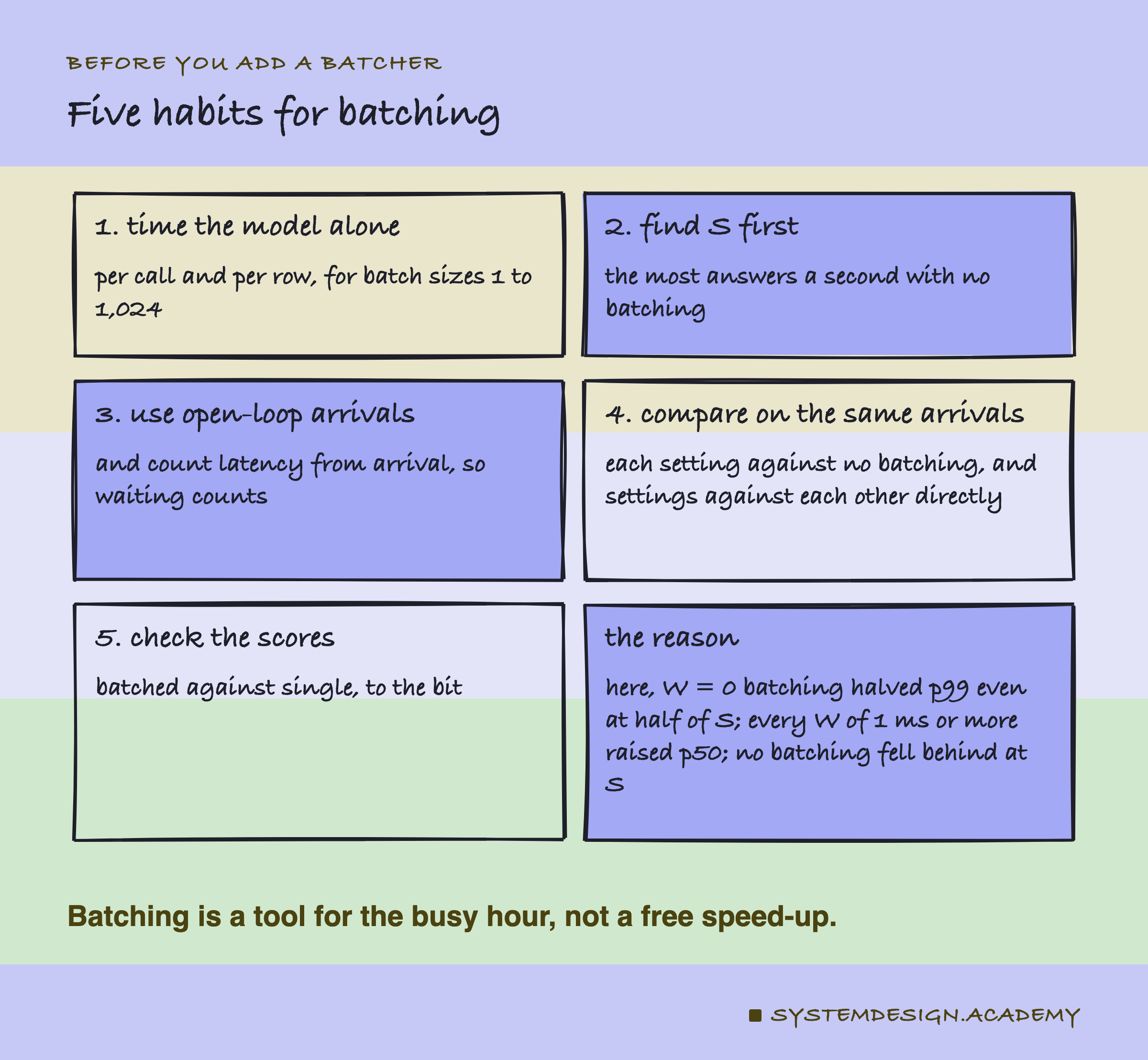
If you take one thing to work on Monday, time your model on 1, 8, 32 and 1,024 rows. It takes a few minutes, and it tells you whether batching can help at all.

If it can, find the most answers a second your service gives with no batching, then try a batcher with no timed wait and a cap of 32, on the same random arrivals. On this box that one change kept the service up at 2.5 times its old limit and halved its p99 even when it was half busy.

The one idea to keep: batching pays for the fixed cost of a call once instead of many times. Waiting on purpose to fill a batch is a separate choice, and it costs every quiet request. Measure both on your own model and hardware.