Serving And Inference

Tail Latency: What Sits in the Slowest 1% of Requests

0 of 33 complete

0%

Contents

Back|Serving And InferenceTail Latency: What Sits in the Slowest 1% of Requests
1/33
84 min left
  1. Home
  2. AI Engineering: Data, RAG and Agents
  3. Serving and Inference Basics
  4. Tail Latency: What Sits in the Slowest 1% of Requests
Prerequisites
Latency Anatomy: Where the Time in One Prediction Request GoesrequiredBatch or Online Scoring: A Month-Old Score Cost Nothing I Could Measure HererequiredWhat a Feature Is: A Better Model or a Better Feature?required
Related Topics
Model Signatures: The Right Numbers in the Wrong Shape, and What a Schema Check CatchesPackaging, Registry and Versioning
1 of 33
Previous lessonLatency Anatomy: Where the Time in One Prediction Request Goes

System Design

  • Foundation
  • Intermediate
  • Advanced
  • Capstone

AI Engineering

  • Foundation
  • Data, RAG and Agents
  • Evaluation, LLM Ops and Security

systemdesign.academy

  • Home
  • Glossary
  • Interview prep
  • Reviews
  • About
  • Privacy
  • Terms

The Bus That Is Late Once in a Hundred Days

Let me start with a bus.

Imagine you take the same bus to work every morning. Most mornings the ride takes about twenty minutes. On a few mornings it takes twenty-five. And about one morning in a hundred, something odd happens: the driver changes, a road is closed, the doors stick, and the ride takes an hour.

A flat illustration of a smiling man in glasses, a light blue shirt and dark trousers, with a brown bag over his shoulder, like someone on his way to work. Below the picture: most mornings the bus takes about twenty minutes; about one morning in a hundred, it takes an hour; "usually twenty minutes" is true, and it hides the morning that made you late.

If a friend asks "how long is your ride?", you say "twenty minutes". That answer is true for most days. But it hides the one bad morning, and the bad morning is the one you remember, because it made you late.

Now imagine your day needs ten buses, one after another. Each bus is late only one day in a hundred. How often is at least one of the ten late? If the buses are late for separate reasons, almost one day in ten. If they are late for the same reason, for example snow, they tend to be late on the same days, and the answer changes. Keep that thought: it comes back near the end with real numbers.

A prediction service is like that bus line. Most answers come back quickly. A few come back slowly. In this lesson I send a real service 100,000 requests, five times over. Then I look closely at the slow few: how slow they are, what they have in common, and what happens when a page needs ten answers.

Where This Lesson Starts

This is lesson 3 of the chapter on serving a model. Lesson 2, latency anatomy, took one request apart and timed every step inside it. It found that a normal request took about one millisecond, and that the model's predict_proba was the biggest step. It looked at the typical request. This lesson looks at the slow ones.

I use the same model, the same service and the same kind of rented machine as lesson 2, so I do not explain them again. In short: the model is the features chapter's gradient boosted tree model. It scores one customer of a real online shop at the start of a month. It scored a test AP of 0.5450.

AP, average precision, is a score from 0 to 1 for how well the model ranks the real buyers above the others. "Test" means it was measured on months the model never trained on. The service is a small web service built with FastAPI and uvicorn, and it reads the customer's six features from a SQLite table. If any of that is new, please read lesson 2 first.

The question for this lesson is simple to ask. Why is the time of the slowest 1 in 100 requests far from the time of the typical one, and what sits in that slow group? Before I measured, I had a confident answer: Python's garbage collector. You will see that the box disagreed.

The Words You Need First

Please read this slide slowly if any word is new. Every slide after it uses these words.
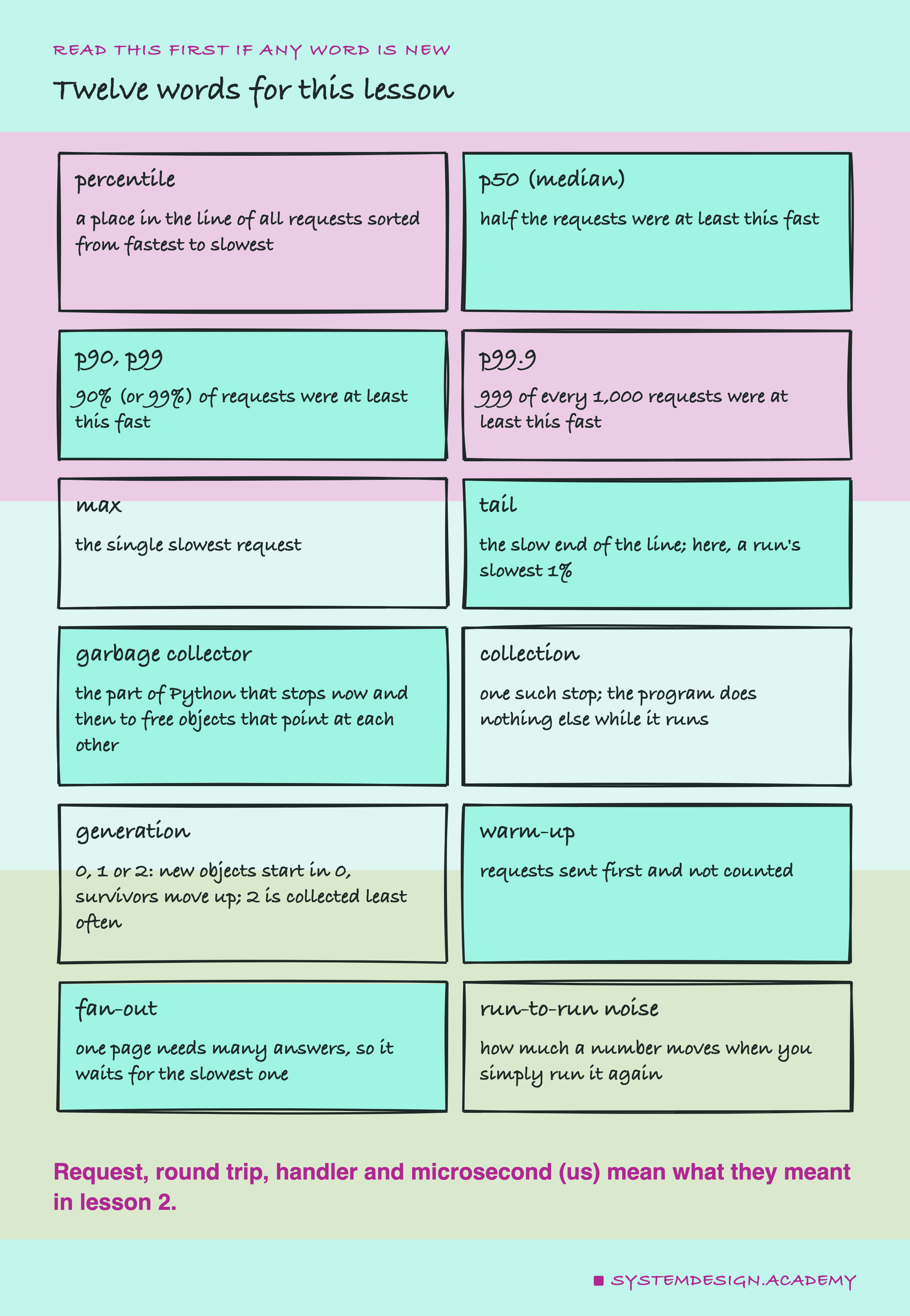
A hand-drawn grid of twelve cards, two per row. Percentile: a place in the line of all requests sorted from fastest to slowest. p50 (median): half the requests were at least this fast. p90, p99: 90% (or 99%) of requests were at least this fast. p99.9: 999 of every 1,000 requests were at least this fast. Max: the single slowest request. Tail: the slow end of the line; here, a run's slowest 1%. Garbage collector: the part of Python that stops now and then to free objects that point at each other. Collection: one such stop; the program does nothing else while it runs. Generation: 0, 1 or 2; new objects start in 0, survivors move up; 2 is collected least often. Warm-up: requests sent first and not counted. Fan-out: one page needs many answers, so it waits for the slowest one. Run-to-run noise: how much a number moves when you simply run it again. Below: request, round trip, handler and microsecond (us) mean what they meant in lesson 2.

Think of a school race with 100 children. Line them up from the fastest to the slowest. The child in the middle, number 50, ran the median time, also called the p50. The child at number 90 ran the p90: 90 children were at least that fast. The child at number 99 ran the p99, and only one child was slower. With 1,000 children, the p99.9 is the time of child number 999. The very last child ran the max. A percentile is any of these places in the line.

The slow end of the line is the tail. Tail means the times out in that slow end, usually the p99 and beyond. In this lesson "the tail" of a run means its slowest 1% of requests, and "the deep tail" its slowest 0.1%.

Python cleans up memory in two ways. Most objects are freed the moment nothing uses them any more. Python counts the users of every object, and the count reaching zero frees it. A few objects point at each other in a circle, so their count never reaches zero on its own. The garbage collector is the part of Python that stops now and then to find those circles and free them. Each stop is a collection, and the program does nothing else while it runs.

Python sorts objects into three generations. New objects start in generation 0, and objects that survive a collection move to an older one. Generation 0 is collected often and quickly, generation 2 rarely and slowly.

The Headline: A Short Tail, and One Request Far Out

Here is the main result first. I sent 100,000 requests, one at a time, to a fresh service, and did that five times. This chart lines up every request of each run from fastest to slowest.
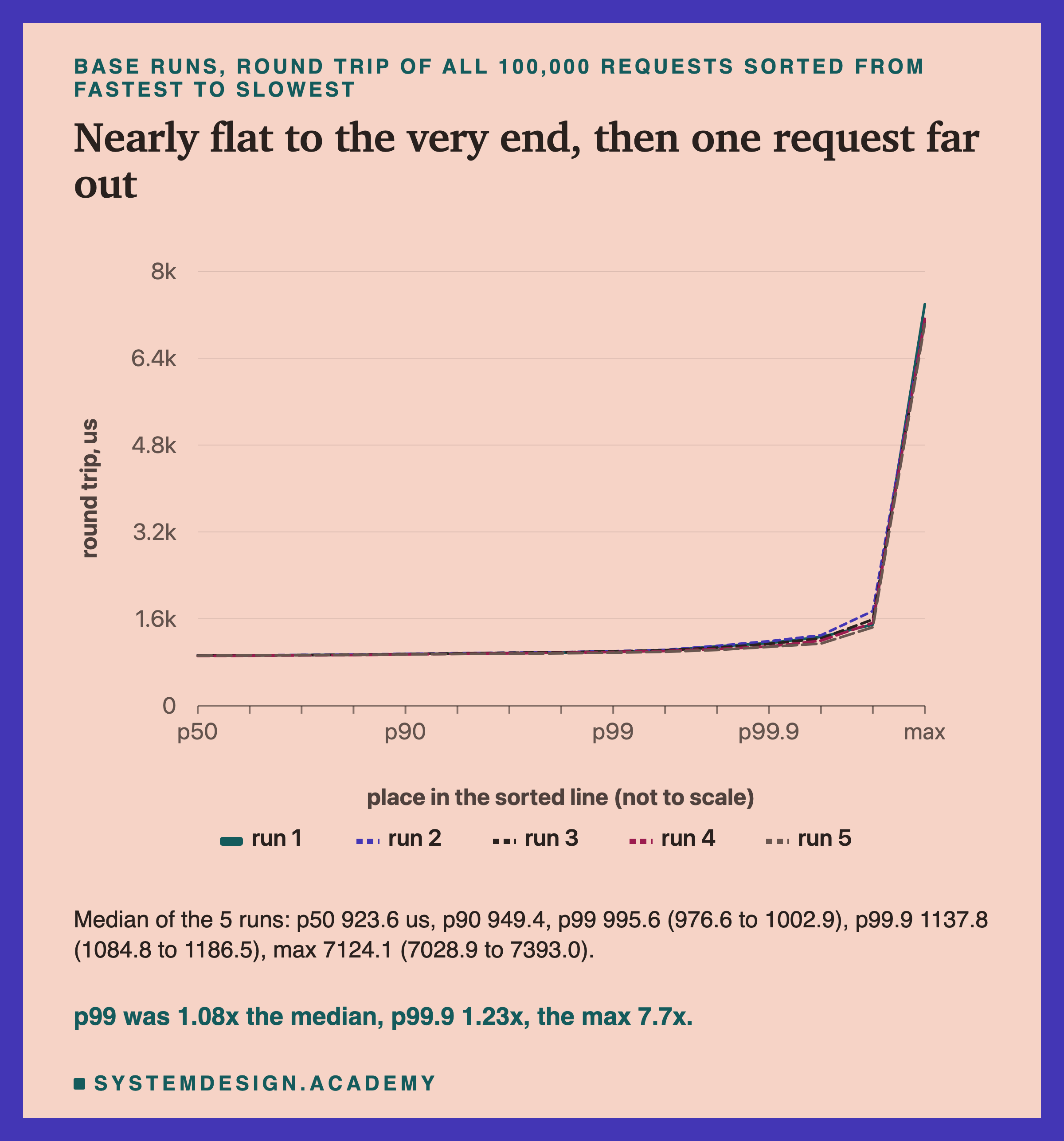
A line chart of the round trip in microseconds against the place in the sorted line of 100,000 requests, with five lines, one per run, nearly on top of each other. The x axis is not to scale and is marked p50, p90, p99, p99.9 and max. The lines are almost flat from p50 to p99.9, near 1,000 us, then shoot up to about 7,000 us at the max. Below: median of the 5 runs, p50 923.6 us, p90 949.4, p99 995.6 (976.6 to 1002.9), p99.9 1137.8 (1084.8 to 1186.5), max 7124.1 (7028.9 to 7393.0). Caption: p99 was 1.08x the median, p99.9 1.23x, the max 7.7x.

The median round trip was 923.6 microseconds. The p90 was 949.4 and the p99 995.6. So on this quiet box, with one request at a time, the slowest 1 in 100 requests took only about 8% longer than the typical one. The p99.9, the slowest 1 in 1,000, was 1,137.8 microseconds, 1.23 times the median.

The max was 7,124.1 microseconds, 7.7 times the median. It was far out on its own, and later slides show that it was the same request in every run: the very first one.

The numbers in brackets are the lowest and highest of the five runs. Notice how they grow towards the tail. The five medians were all between 916.0 and 924.0. The five p99.9 values were between 1,084.8 and 1,186.5, a spread of about 100 microseconds. The further out you look, the fewer requests a number rests on. The p99.9 of 100,000 requests rests on only the 100 slowest, so it moves more from run to run. That is why I ran everything five times.

So, in this setup, is p99 "far" from the median? No. It was close. The far requests were at the very end. The rest of the lesson asks what those slow requests had in common, and which changes moved them.

How the Lab Was Built

I wrote the lab's design into the docstring of scripts/labs/serving/tail_latency.py on 2026-10-02, before any timed run. It names every measurement, every change, the rule for "told apart from noise", and seven guesses.
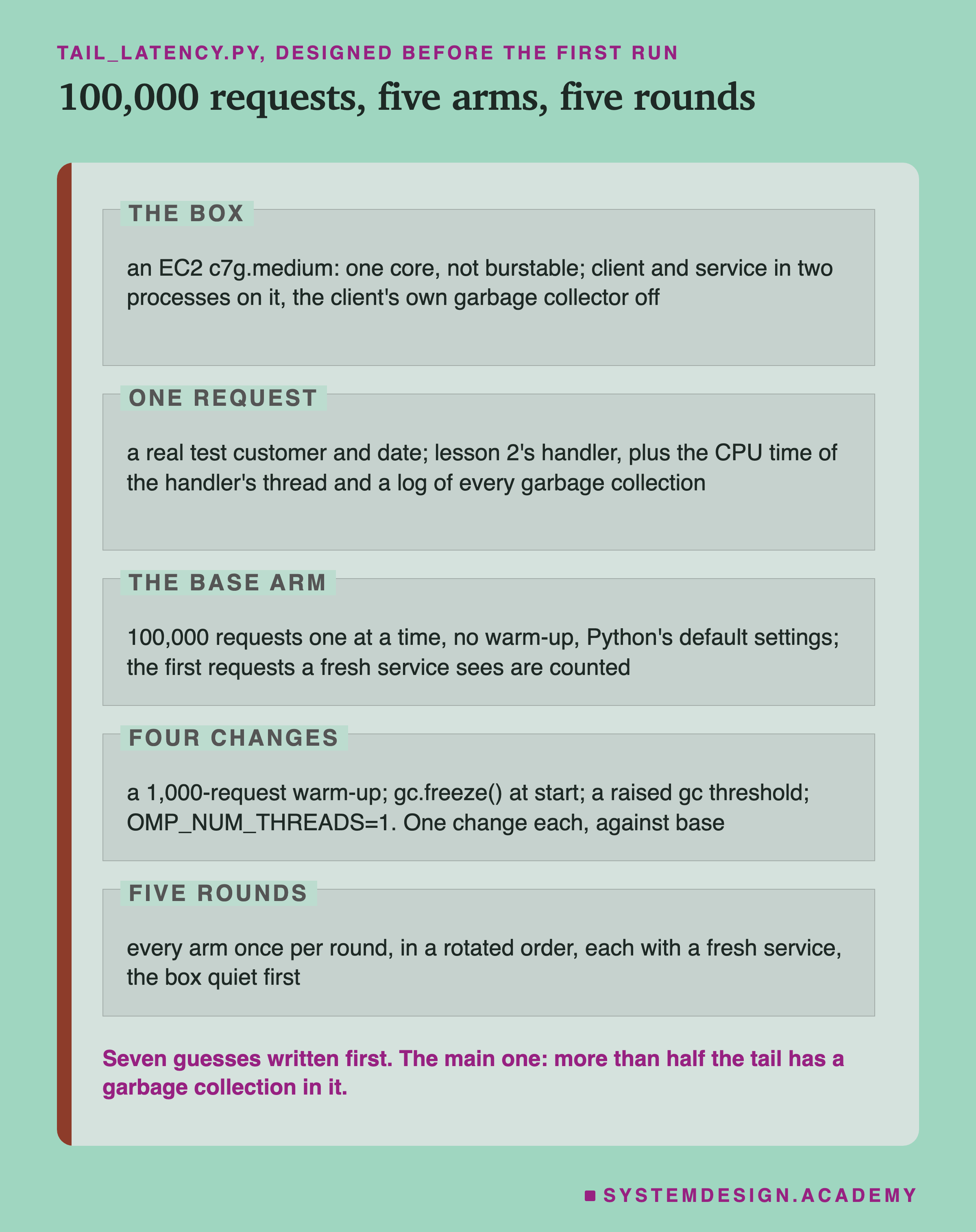
A page in five labelled zones, titled 100,000 requests, five arms, five rounds. The box: an EC2 c7g.medium, one core, not burstable; client and service in two processes on it, the client's own garbage collector off. One request: a real test customer and date; lesson 2's handler, plus the CPU time of the handler's thread and a log of every garbage collection. The base arm: 100,000 requests one at a time, no warm-up, Python's default settings; the first requests a fresh service sees are counted. Four changes: a 1,000-request warm-up; gc.freeze() at start; a raised gc threshold; OMP_NUM_THREADS=1; one change each, against base. Five rounds: every arm once per round, in a rotated order, each with a fresh service, the box quiet first. Caption: seven guesses written first; the main one, more than half the tail has a garbage collection in it.

The base arm is the plain service with Python's default settings. It gets no warm-up: the first of its 100,000 counted requests is the first request the fresh service ever answers. I wanted the first requests inside the measurement, so I could see what they do to the tail.

Four changes, one at a time. An arm is one version of the setup. Each of the four other arms changes exactly one thing from base. The warm arm sends 1,000 requests first and does not count them. The freeze arm calls gc.freeze() when the service starts. Python's docs say it moves every object the collector tracks into "a permanent generation" and ignores them "in all the future collections". The thresh arm raises the collector's first limit from 2,000 to 50,000, so generation 0 is collected far less often. The omp1 arm sets OMP_NUM_THREADS=1, the number of threads the model may use.

Five rounds. Each round runs all five arms, each with a fresh service, in an order that rotates from round to round. So no arm always runs first or last. Then I compare each arm with base in the same round.

The Machine, and Lesson 2's Shared Core

Like lesson 2, every timing comes from a small machine I rented from Amazon Web Services, never from my laptop, which is always busy with other work.
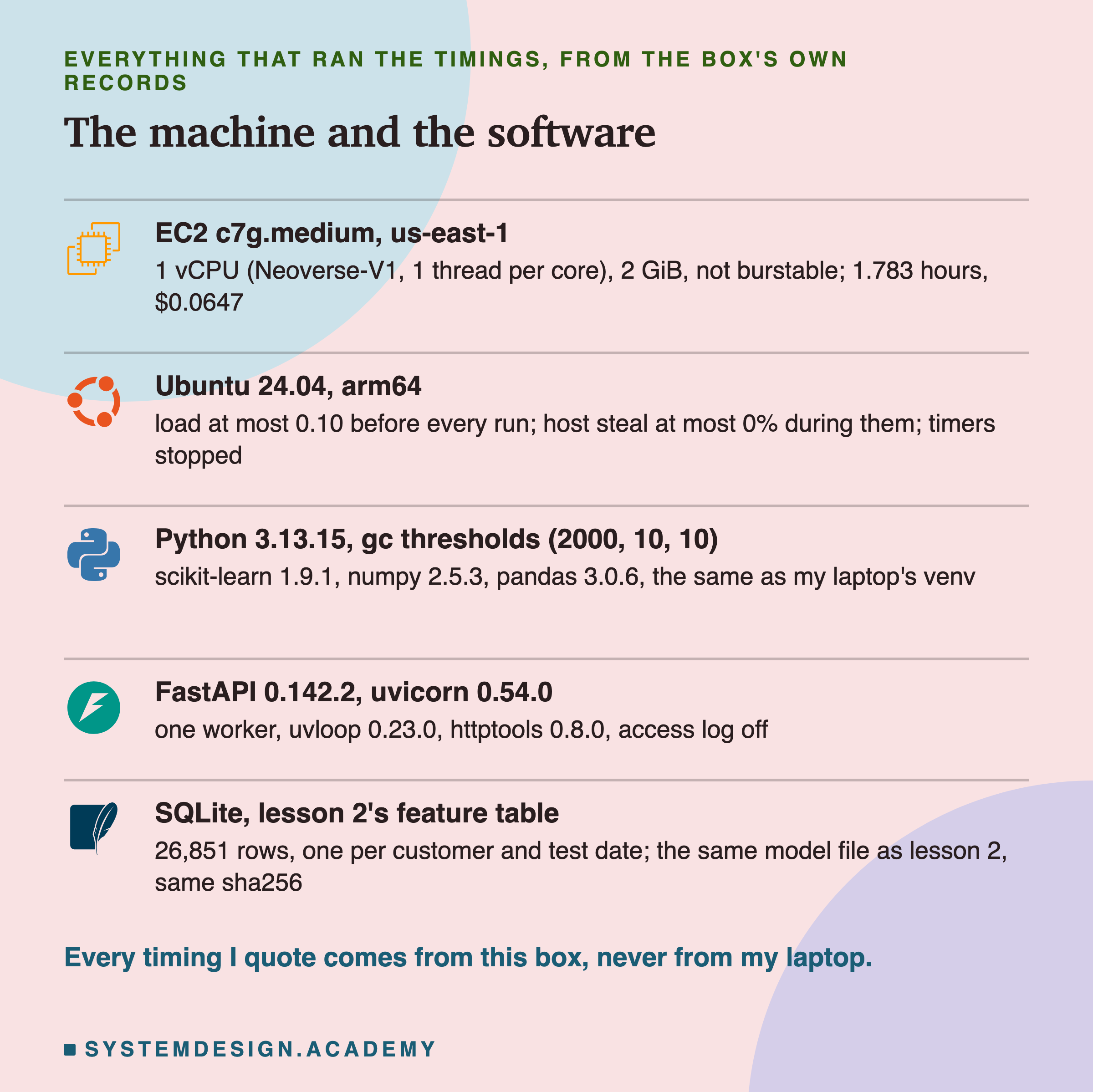
Five rows, each with a logo. EC2 c7g.medium, us-east-1: 1 vCPU (Neoverse-V1, 1 thread per core), 2 GiB, not burstable; 1.783 hours, $0.0647. Ubuntu 24.04, arm64: load at most 0.10 before every run; host steal at most 0% during them; timers stopped. Python 3.13.15, gc thresholds (2000, 10, 10): scikit-learn 1.9.1, numpy 2.5.3, pandas 3.0.6, the same as my laptop's venv. FastAPI 0.142.2, uvicorn 0.54.0: one worker, uvloop 0.23.0, httptools 0.8.0, access log off. SQLite, lesson 2's feature table: 26,851 rows, one per customer and test date; the same model file as lesson 2, same sha256. Caption: every timing I quote comes from this box, never from my laptop.

The box is an EC2 c7g.medium. AWS lists it with 1 virtual CPU and 2 GiB of memory, and its processor is an AWS Graviton3. My account allows only one virtual CPU of this kind at a time, so the client and the service share that one core, as in lesson 2.

Lesson 2's review found a problem with that. The client's own work landed in "outside the handler". And the time to read the request body had two humps, likely because Python's http.client sends the headers and the body in two pieces. This lab was designed around that before it ran, in four ways:

  1. The client is its own process, and it writes each request in one piece, headers and body together. Lesson 2 saw two humps in the body read. Here, in all 25 runs, only 0.001% to 0.008% of requests took over 50 microseconds to read the body, against 36% to 39% in lesson 2. That is a different client in a different setup, so it shows the humps are gone here, not exactly why.

  2. The client's garbage collector is off while it sends, so it cannot pause the timing loop. A hook counts any collection that still happens, and it counted 0 in all 25 runs.

  3. The tail is found from the round trip, but explained on the service's own clock. The handler's work, from "body in hand" to "answer ready", never waits for the client. Its thread's CPU time shows when the service itself was not running.

The Whole Lab in One Picture

Before the recordings, here is the whole lab as one numbered sequence. The numbers on the arrows match the numbers on the recordings that follow.
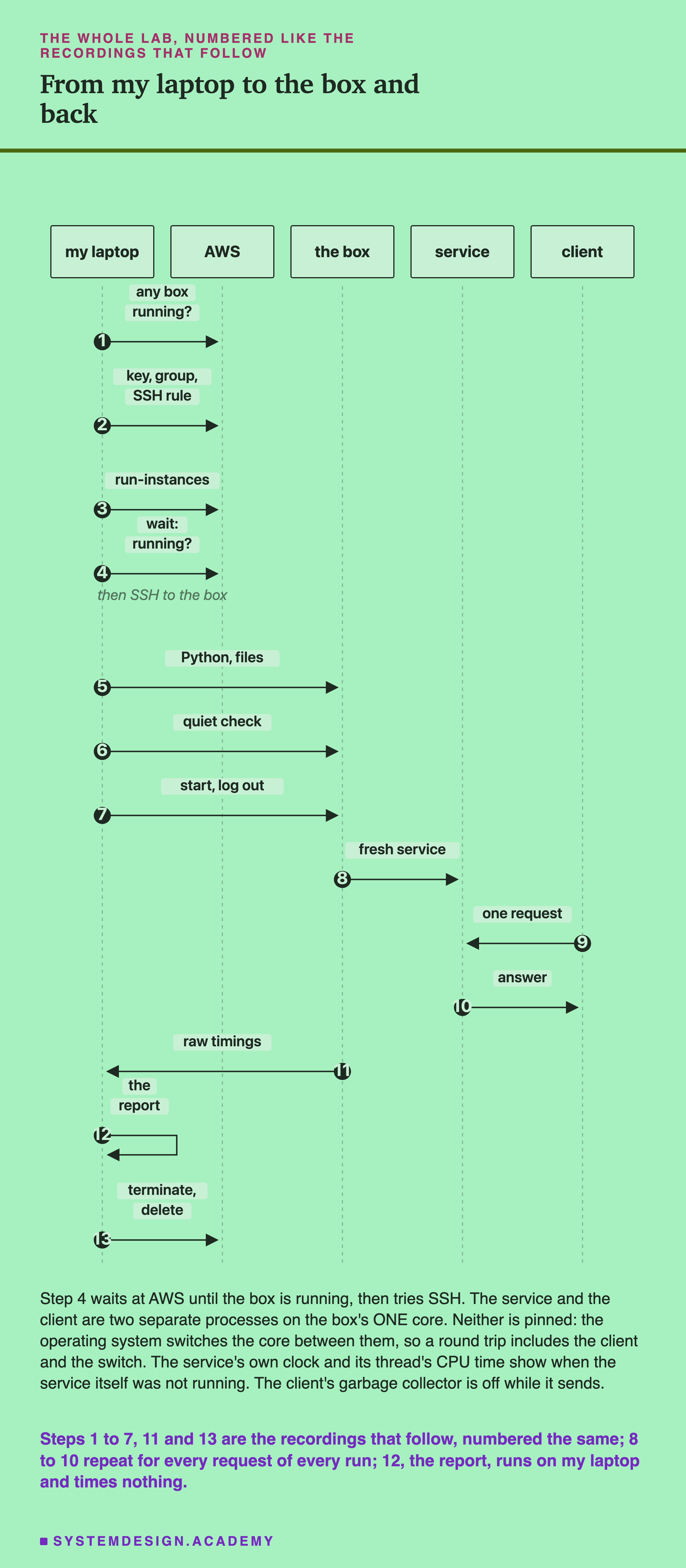
A sequence diagram with five lifelines: my laptop, AWS, the box, service and client, and thirteen numbered arrows. 1, my laptop asks AWS whether any box is running. 2, my laptop creates a key, a group and an SSH rule at AWS. 3, run-instances. 4, my laptop asks AWS, wait: running?, with the note then SSH to the box. 5, my laptop sends Python and the files to the box. 6, quiet check. 7, start, log out. 8, the box starts a fresh service. 9, the client sends one request to the service. 10, the service sends the answer to the client. 11, the box sends the raw timings to my laptop. 12, the report, an arrow from my laptop to itself. 13, my laptop tells AWS to terminate and delete. Below: step 4 waits at AWS until the box is running, then tries SSH; the service and the client are two separate processes on the box's one core; neither is pinned; the operating system switches the core between them, so a round trip includes the client and the switch; the service's own clock and its thread's CPU time show when the service itself was not running; the client's garbage collector is off while it sends. Caption: steps 1 to 7, 11 and 13 are the recordings that follow, numbered the same; 8 to 10 repeat for every request of every run; 12, the report, runs on my laptop and times nothing.

Steps 1 to 7 happen once: check, rent the box, set it up, and start the runs. Steps 8 to 10 repeat for every request of every run, 2,505,000 requests in all, warm-up included, with nobody connected. Step 11 brings the raw timings home, step 12 does the arithmetic on my laptop, and step 13 deletes everything.

Is anything pinned to the core? No. Pinning means telling the operating system to run a program only on certain cores. With one core there is nothing to choose: the service process and the client process take turns on the same core. When the client sends a request, the operating system stops the client and runs the service. When the service answers, it switches back. That switch is inside every round trip. It is the same in every arm, so it cannot explain a difference between arms.

Build the Lab Box Yourself

Lesson 2 rented a box and only told you about it. This time I show every step, so you can rent the same kind of box and run the same lab. The flow figure above numbers the steps, and each recording below carries the same number.

The path to follow. All the steps live in one file, scripts/labs/serving/tail_files/tail_aws_steps.sh. From the scripts/labs/serving folder, run bash tail_files/tail_aws_steps.sh check, then access, launch, wait, copy, quiet, start, fetch and, at the end, teardown. The code blocks on these slides are that file's lines, copied exactly, so you can read what each step does. If you would rather paste them by hand, paste the variables block below first, in the same terminal. Each step also saves the box's id, group id and address to a small file, so the steps work in separate terminals too.

cd scripts/labs/serving
export AWS_DEFAULT_REGION=us-east-1 AWS_PAGER=""
NAME=ai-research-course-tail
STATE=~/lab-data/serving/tail/walk
KEY=~/lab-data/serving/keys/$NAME.pem
SSH=(-i "$KEY" -o LogLevel=ERROR -o StrictHostKeyChecking=accept-new -o "UserKnownHostsFile=$STATE/known_hosts")
ROUNDS=${ROUNDS:-5}; N_WARM=${N_WARM:-1000}; N_MEASURED=${N_MEASURED:-100000}
mkdir -p "$STATE"
touch "$STATE/vars"; . "$STATE/vars"

What you need first. An AWS account, the AWS command line tool (aws) set up with your keys for the region us-east-1, and , , and . The region needs a , the ready-made private network that new accounts get; step 2 puts the box's door rule in it. Step 5 copies two things that must already be on your computer. The first is lesson 2's prepared files in , made by in this folder. The second is the shop data in , made by .

Steps 1 to 3: Check, Lock the Door, Rent the Box

Step 1: is any other course box running? My account allows one small box of this kind at a time, and another lesson may be using it. So the first command counts the course's boxes that are not yet deleted. It must print 0. While I was writing this slide, it printed 1: another lesson's box was running, so I would have had to wait.
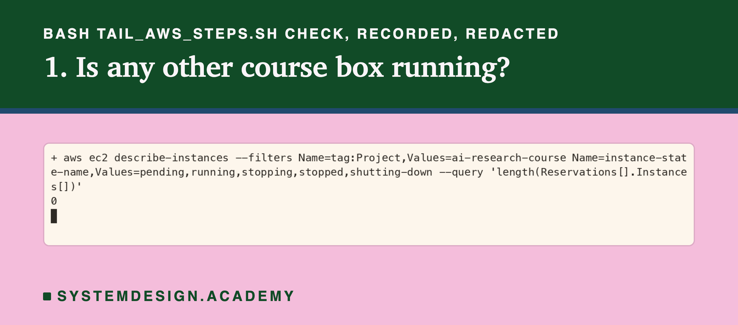
A real terminal recording of step 1. The shell prints the command aws ec2 describe-instances with filters for the tag Project=ai-research-course and the states pending, running, stopping, stopped and shutting-down, asking for the number of instances; the answer is 0.

aws ec2 describe-instances --filters "Name=tag:Project,Values=ai-research-course" \
  "Name=instance-state-name,Values=pending,running,stopping,stopped,shutting-down" \
  --query "length(Reservations[].Instances[])"

Step 2: a key and a locked door. A key pair is how you prove to the box that you are allowed in. AWS keeps one half, and you keep the other half in a file that only you can read. A security group is a door rule for the box. Mine opens only port 22, the SSH port, and only to my own address, so nobody else on the internet can even knock.
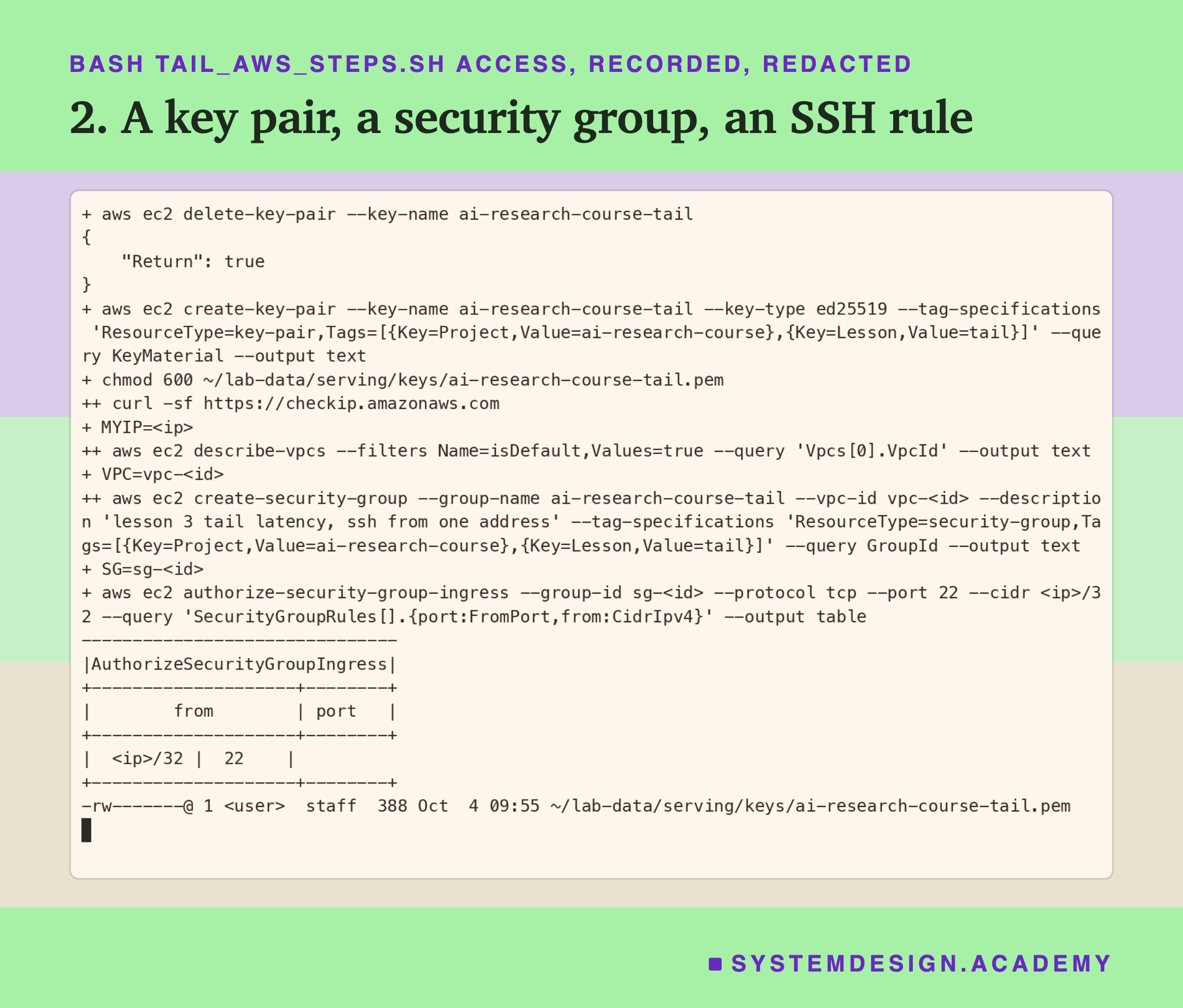
A real terminal recording of step 2, with the address, network and group ids replaced by placeholders. delete-key-pair for ai-research-course-tail returns true; create-key-pair writes the key material to the key file without printing it; chmod 600 on the key file; curl reads my address; describe-vpcs finds the default network; create-security-group makes the group ai-research-course-tail with its tags; authorize-security-group-ingress prints a small table: from my address /32, port 22. Last line: the key file, readable only by its owner, 388 bytes.

aws ec2 delete-key-pair --key-name "$NAME"       # an old pair of the same name, if any (no error if none)
mkdir -p "$(dirname "$KEY")"
aws ec2 create-key-pair --key-name "$NAME" --key-type ed25519 \
  --tag-specifications "ResourceType=key-pair,Tags=[{Key=Project,Value=ai-research-course},{Key=Lesson,Value=tail}]" \
  --query KeyMaterial --output text > "$KEY"
chmod 600 "$KEY"
MYIP=$(curl -sf https://checkip.amazonaws.com)
VPC=$(aws ec2 describe-vpcs --filters Name=isDefault,Values=true --query "Vpcs[0].VpcId" --output text)
SG=$(aws ec2 create-security-group --group-name "$NAME" --vpc-id "$VPC" \
  --description "lesson 3 tail latency, ssh from one address" \
  --tag-specifications "ResourceType=security-group,Tags=[{Key=Project,Value=ai-research-course},{Key=Lesson,Value=tail}]" \
  --query GroupId --output text)
aws ec2 authorize-security-group-ingress --group-id "$SG" --protocol tcp --port 22 --cidr "$MYIP/32" \
  --query "SecurityGroupRules[].{port:FromPort,from:CidrIpv4}" --output table
echo "SG=$SG" >> "$STATE/vars"
ls -l "$KEY"

Steps 4 to 7: Wait, Set Up, Check It Is Quiet, Start

Step 4: wait until it runs. A new box takes a short while to start. The AWS tool can wait for you. Then the step reads the box's public address, and tries SSH every five seconds until the box answers.
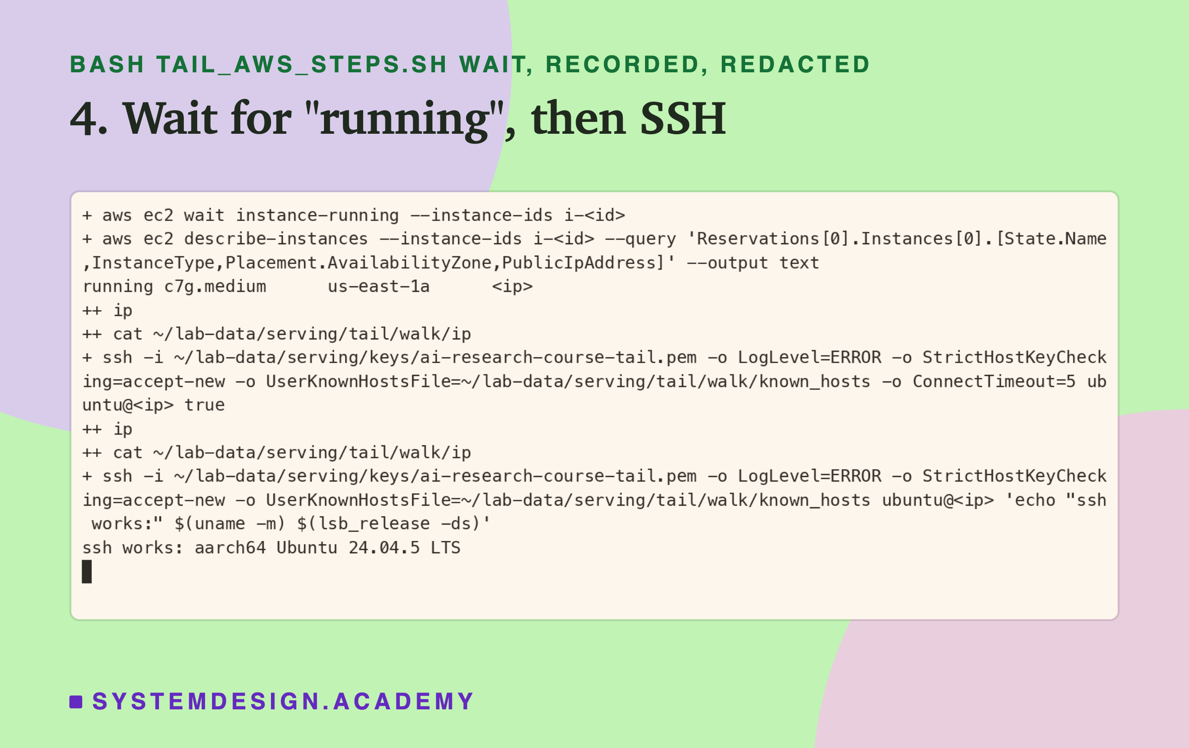
A real terminal recording of step 4, with the instance id and address replaced by placeholders. aws ec2 wait instance-running, then describe-instances prints running, c7g.medium, us-east-1a and the address. Then ssh to the box, which answers: ssh works, aarch64, Ubuntu 24.04.5 LTS.

aws ec2 wait instance-running --instance-ids "$ID"
IP=$(aws ec2 describe-instances --instance-ids "$ID" \
  --query "Reservations[0].Instances[0].PublicIpAddress" --output text)
echo "IP=$IP" >> "$STATE/vars"
until ssh "${SSH[@]}" -o ConnectTimeout=5 ubuntu@"$IP" true 2>/dev/null; do sleep 5; done
ssh "${SSH[@]}" ubuntu@"$IP" 'echo "ssh works:" $(uname -m) $(lsb_release -ds)'

Step 5: Python and the lab files. The box gets the same Python, 3.13.15, and the same pinned library versions as lesson 2, through uv, a fast installer for Python. Then the lab files go over with scp, a copy command that works through SSH. They are lesson 2's model file, feature table, request list and service. Then come the features chapter's task files and shop data, and this lesson's own files. The last command builds the SQLite table on the box and prints the files' sha256 fingerprints, so you can check they match the ones on your computer.
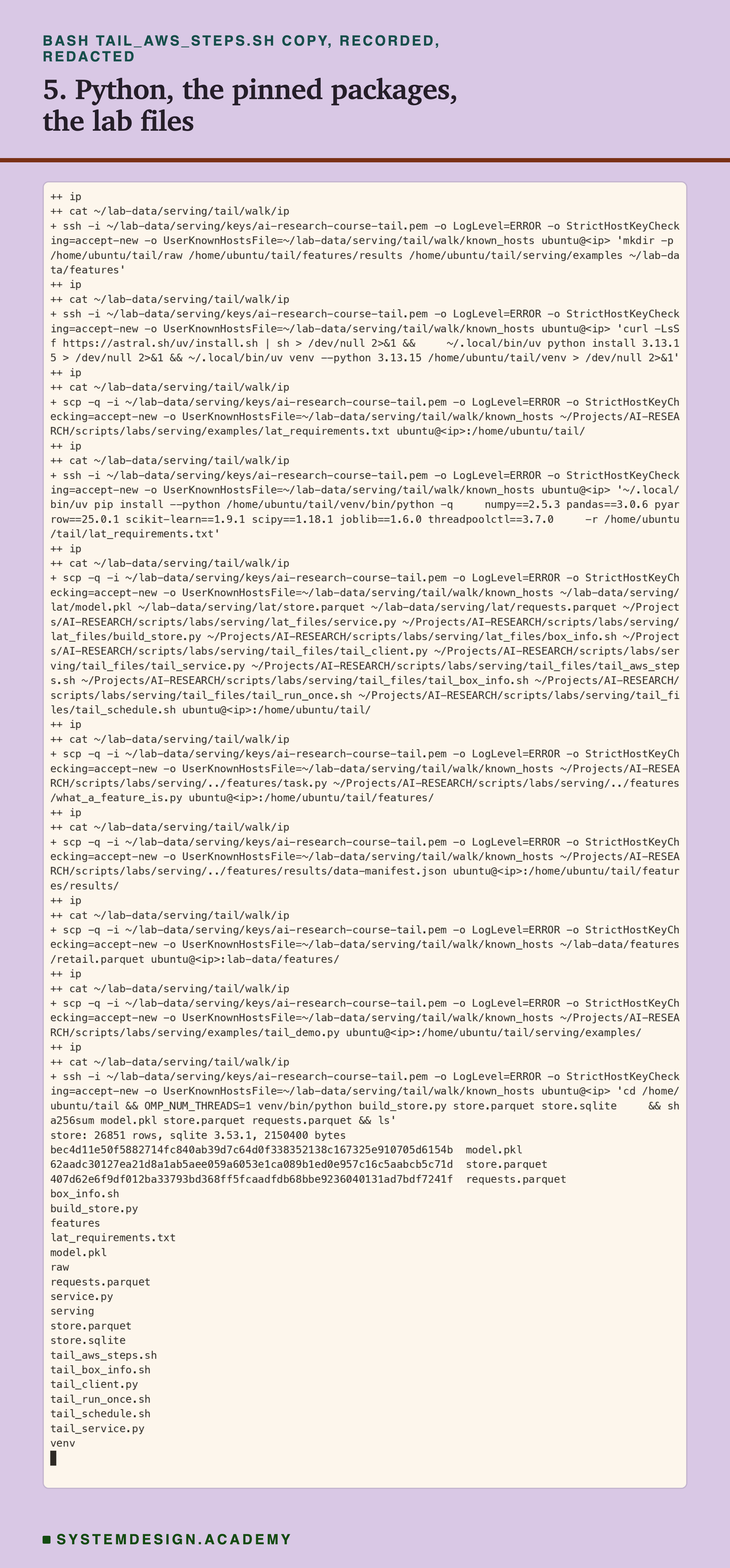
A real terminal recording of step 5, with the address replaced by a placeholder. Over ssh: make the folders; install uv, Python 3.13.15 and a fresh venv; copy lat_requirements.txt and install the pinned versions of numpy, pandas, pyarrow, scikit-learn, scipy, joblib and threadpoolctl with it. Then scp copies lesson 2's model.pkl, store.parquet, requests.parquet, service.py, build_store.py and box_info.sh, this lesson's tail files, the features chapter's task files, the shop data and tail_demo.py. Last: build_store.py prints store, 26851 rows, sqlite 3.53.1, 2150400 bytes; the sha256 of model.pkl starts bec4d11e, of store.parquet 62aadc30, of requests.parquet 407d62e6; then the list of files in the folder.

ssh "${SSH[@]}" ubuntu@"$IP" "mkdir -p tail/raw tail/features/results tail/serving/examples lab-data/features"
ssh "${SSH[@]}" ubuntu@"$IP" "curl -LsSf https://astral.sh/uv/install.sh | sh > /dev/null 2>&1 && \
  ~/.local/bin/uv python install 3.13.15 > /dev/null 2>&1 && ~/.local/bin/uv venv --python 3.13.15 tail/venv > /dev/null 2>&1"
scp -q "${SSH[@]}" examples/lat_requirements.txt ubuntu@"$IP":tail/
ssh "${SSH[@]}" ubuntu@"$IP" "~/.local/bin/uv pip install --python tail/venv/bin/python -q \
  numpy==2.5.3 pandas==3.0.6 pyarrow==25.0.1 scikit-learn==1.9.1 scipy==1.18.1 joblib==1.6.0 threadpoolctl==3.7.0 \
  -r tail/lat_requirements.txt"
scp -q "${SSH[@]}" ~/lab-data/serving/lat/model.pkl ~/lab-data/serving/lat/store.parquet \
  ~/lab-data/serving/lat/requests.parquet lat_files/service.py lat_files/build_store.py lat_files/box_info.sh \
  tail_files/tail_*.py tail_files/tail_*.sh ubuntu@"$IP":tail/
scp -q "${SSH[@]}" ../features/task.py ../features/what_a_feature_is.py ubuntu@"$IP":tail/features/
scp -q "${SSH[@]}" ../features/results/data-manifest.json ubuntu@"$IP":tail/features/results/
scp -q "${SSH[@]}" ~/lab-data/features/retail.parquet ubuntu@"$IP":lab-data/features/
scp -q "${SSH[@]}" examples/tail_demo.py ubuntu@"$IP":tail/serving/examples/
ssh "${SSH[@]}" ubuntu@"$IP" "cd tail && OMP_NUM_THREADS=1 venv/bin/python build_store.py store.parquet store.sqlite \
  && sha256sum model.pkl store.parquet requests.parquet && ls"

Steps 11 and 13: Bring the Timings Home, Then Delete Everything

Steps 8 to 10 in the flow figure happen on the box, once for every request of every run, with nobody watching. Step 12 is the report on my laptop. That leaves two recorded steps.

Step 11: bring the timings home first. The first box I rented for this lesson ran every run, and then it was deleted before anyone copied the results off it. Everything it measured was lost. So the rule now is: the moment the runs finish, copy the raw files back, before you do anything else.
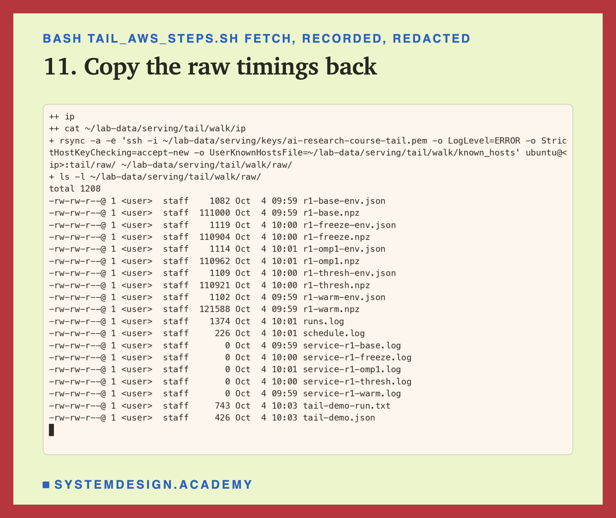
A real terminal recording of step 11, with the address and user name replaced by placeholders. rsync copies the box's tail/raw folder to my laptop, then ls -l lists what arrived: an npz file and an env.json file for each of the five arms of the short schedule, runs.log, schedule.log, five empty service logs, tail-demo-run.txt of 743 bytes and tail-demo.json of 426 bytes.

rsync -a -e "ssh ${SSH[*]}" ubuntu@"$IP":tail/raw/ "$STATE/raw/"
ls -l "$STATE/raw/"

Step 13: delete the box, the key and the door rule, and check. A box you forget keeps costing money. The step deletes the box, waits until AWS says "terminated", then deletes the key pair and the security group. The security group can only be deleted once the box is fully gone, so the step retries that command every ten seconds until AWS accepts it. The last four commands ask AWS again. Each count must be 0: boxes still running with this lesson's tag, key pairs and security groups with its name, and disks with its tag.
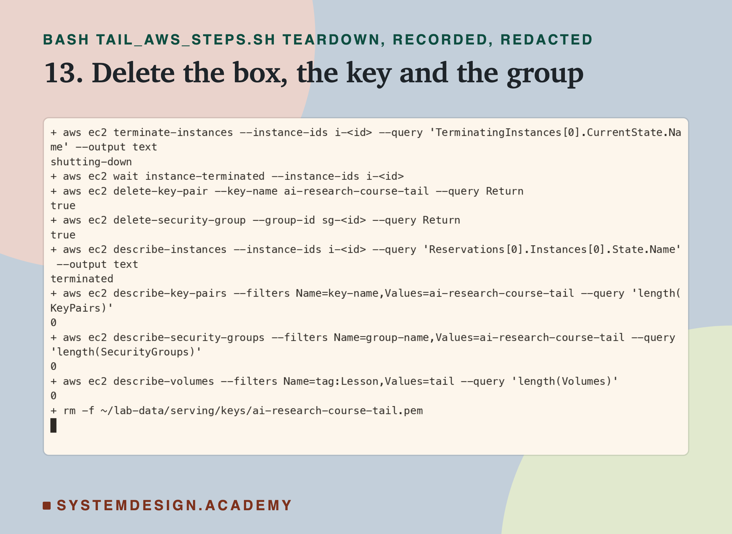
A real terminal recording of step 13, with the instance and group ids replaced by placeholders. terminate-instances prints shutting-down; wait instance-terminated; delete-key-pair prints true; delete-security-group prints true. Then the checks: describe-instances prints terminated; the count of key pairs named ai-research-course-tail is 0; the count of security groups of that name is 0; the count of volumes tagged Lesson=tail is 0. Last, the key file is removed.

aws ec2 terminate-instances --instance-ids "$ID" --query "TerminatingInstances[0].CurrentState.Name" --output text
aws ec2 wait instance-terminated --instance-ids "$ID"
aws ec2 delete-key-pair --key-name "$NAME" --query Return
until aws ec2 delete-security-group --group-id "$SG" --query Return 2>/dev/null; do sleep 10; done
aws ec2 describe-instances --filters "Name=tag:Lesson,Values=tail" \
  "Name=instance-state-name,Values=pending,running,stopping,stopped,shutting-down" --query "length(Reservations)"
aws ec2 describe-key-pairs --filters "Name=key-name,Values=$NAME" --query "length(KeyPairs)"
aws ec2 describe-security-groups --filters "Name=group-name,Values=$NAME" --query "length(SecurityGroups)"
aws ec2 describe-volumes --filters "Name=tag:Lesson,Values=tail" --query "length(Volumes)"
rm -f "$KEY" "$STATE/vars"

The Lab's Report, Running

This is a real recording of the report script, tail_report.py. It ran on my laptop, but it times nothing. It reads the raw timings the box measured and does all the arithmetic again with its own code.
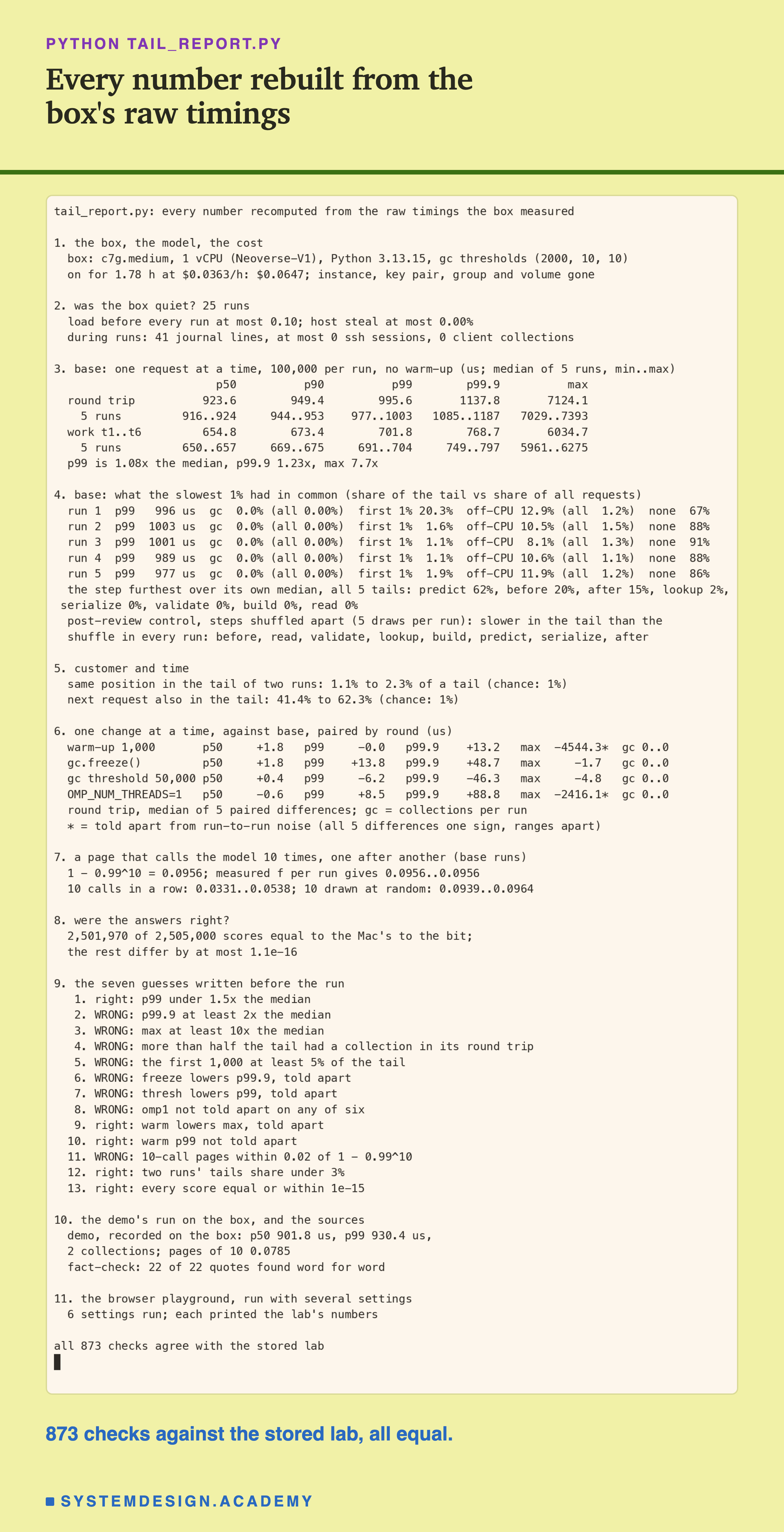
A terminal recording of tail_report.py. Section 1: box c7g.medium, 1 vCPU (Neoverse-V1), Python 3.13.15, gc thresholds (2000, 10, 10); on for 1.78 h at $0.0363 an hour, $0.0647; instance, key pair, group and volume gone. Section 2: 25 runs, load before every run at most 0.10, host steal at most 0.00%, 41 journal lines, at most 0 ssh sessions, 0 client collections. Section 3, base, median of 5 runs and range: round trip p50 923.6 (916 to 924), p90 949.4, p99 995.6 (977 to 1003), p99.9 1137.8 (1085 to 1187), max 7124.1 (7029 to 7393); work t1 to t6 p50 654.8, p99 701.8, p99.9 768.7, max 6034.7; p99 is 1.08x the median, p99.9 1.23x, max 7.7x. Section 4, per run: gc 0.0% of the tail, first 1% 20.3%, 1.6%, 1.1%, 1.1%, 1.9%, off-CPU 12.9%, 10.5%, 8.1%, 10.6%, 11.9%, none 67% to 91%; step furthest over its median, predict 62%, before 20%, after 15%, lookup 2%; a post-review control with the steps shuffled apart, 5 draws per run: slower in the tail than the shuffle in every run, before, read, validate, lookup, build, predict, serialize, after. Section 5: same position in two runs' tails 1.1% to 2.3%; next request also in the tail 41.4% to 62.3%. Section 6: warm-up max minus 4544.3, told apart; OMP_NUM_THREADS=1 max minus 2416.1, told apart; every other difference not told apart; 0 collections per run in every arm. Section 7: 1 - 0.99^10 = 0.0956; 10 calls in a row 0.0331 to 0.0538; 10 at random 0.0939 to 0.0964. Section 8: 2,501,970 of 2,505,000 scores equal to the bit, the rest within 1.1e-16. Section 9: thirteen checks of the seven guesses, five right, eight wrong. Section 10: the demo, p50 901.8 us, p99 930.4 us; 19 of 19 quotes found. Section 11: 6 playground settings. Last line: all 873 checks agree with the stored lab.

The report rebuilds every request's clock readings from the stored files, finds the collections that overlap each request by its own method, and computes its own percentiles. Then it compares 873 numbers and verdicts with the lab's results file, and all of them agreed. If any had not, it would stop with an error.

Section 2 is the quiet check.

Before every run the load average was at most 0.10. Host steal, the CPU time the real machine under my rented box gives to other customers, was 0, and nobody was logged in.

The system log has 41 lines from during the runs. Seven runs each had one small scheduled job start: Ubuntu's statistics collector in four, the hourly jobs in one, a disk check in two. I had stopped the system's timers, but these come from , an older scheduler, which I did not stop. Round 3's omp1 run also had a burst of messages from the management agent. Round 3's warm run had a single line from the network driver. None of that explains the bursts you will see later, which happened in every run.

Five Runs: The Middle Held Still

How much did the five base runs agree?
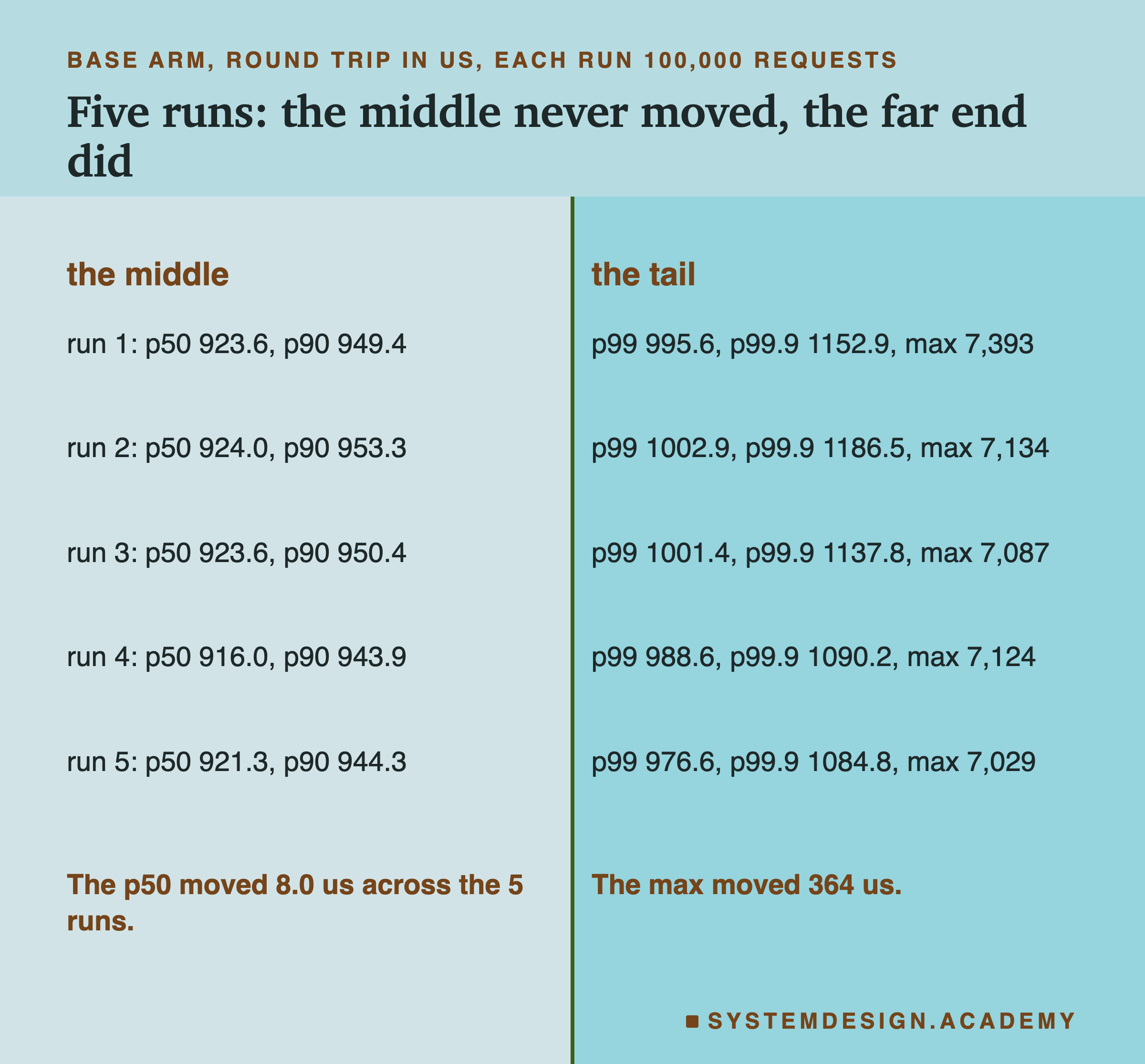
A two-column ledger titled the middle and the tail, one row per base run, round trip in us. Run 1: p50 923.6, p90 949.4; p99 995.6, p99.9 1152.9, max 7,393. Run 2: p50 924.0, p90 953.3; p99 1002.9, p99.9 1186.5, max 7,134. Run 3: p50 923.6, p90 950.4; p99 1001.4, p99.9 1137.8, max 7,087. Run 4: p50 916.0, p90 943.9; p99 988.6, p99.9 1090.2, max 7,124. Run 5: p50 921.3, p90 944.3; p99 976.6, p99.9 1084.8, max 7,029. Below the left column: the p50 moved 8.0 us across the 5 runs. Below the right column: the max moved 364 us.

The p50 moved only 8.0 microseconds across the five runs. The p99 moved 26.4, the p99.9 about 100, and the max 364. This is the normal shape of run-to-run noise. The middle of a distribution rests on tens of thousands of requests and holds still. The far end rests on a few and moves.

This matters for every comparison later in the lesson. If a change moves the p99.9 by 50 microseconds, that is inside the range the same setup moves on its own. So I need a rule, written before the runs, to say when a change is real.

What the Slowest 1% Had in Common

For every request, the lab wrote down several things. Did a garbage collection overlap it? Was it among the first 1% of the run? Was the handler's thread off the core for part of its own work? Then I compared how common each one was in the tail and in all requests.
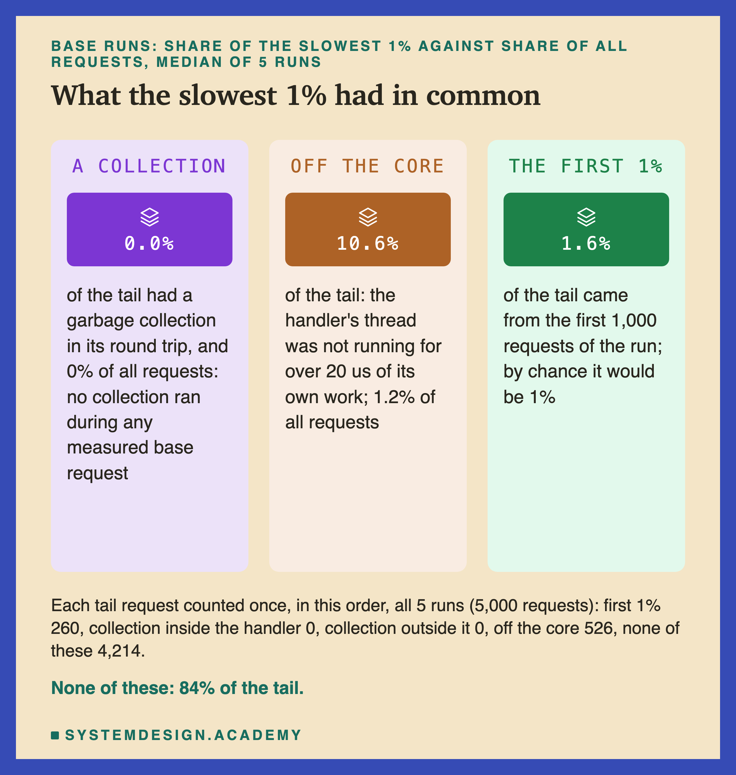
Three panels, base runs, share of the slowest 1% against share of all requests, median of 5 runs. A collection: 0.0% of the tail had a garbage collection in its round trip, and 0% of all requests: no collection ran during any measured base request. Off the core: 10.6% of the tail, the handler's thread was not running for over 20 us of its own work, against 1.2% of all requests. The first 1%: 1.6% of the tail came from the first 1,000 requests of the run; by chance it would be 1%. Below: each tail request counted once, in this order, all 5 runs, 5,000 requests: first 1% 260, collection inside the handler 0, collection outside it 0, off the core 526, none of these 4,214. Caption: none of these, 84% of the tail.

A garbage collection: 0% of the tail. Not a small share. None. No collection ran during any of the 500,000 measured base requests. The next slide explains why.

Off the core: 10.6% of the tail, against 1.2% of all requests. For these requests, the wall clock moved at least 20 microseconds more than the handler's CPU time during its own work. So the core was doing something else for a moment: another process, the operating system, or an interrupt. That attribute is about nine times more common in the tail than overall. But it covers only about one tail request in ten.

The first 1% of the run: 1.6% of the tail, against 1% by chance. In run 1 it was 20.3%, and in the other four runs 1.1% to 1.9%. So the very start of a fresh service mattered in one run and hardly at all in the others. I do not know why run 1 was different.

None of these: 84% of the tail. Counting each tail request once, in the order the design fixed, 4,214 of the 5,000 tail requests had none of the attributes I logged. My list of suspects explained about one slow request in six.

Why the Garbage Collector Never Ran

My main guess was that more than half the tail would have a collection in it. It had none. Before believing a zero, I checked that the hook worked.
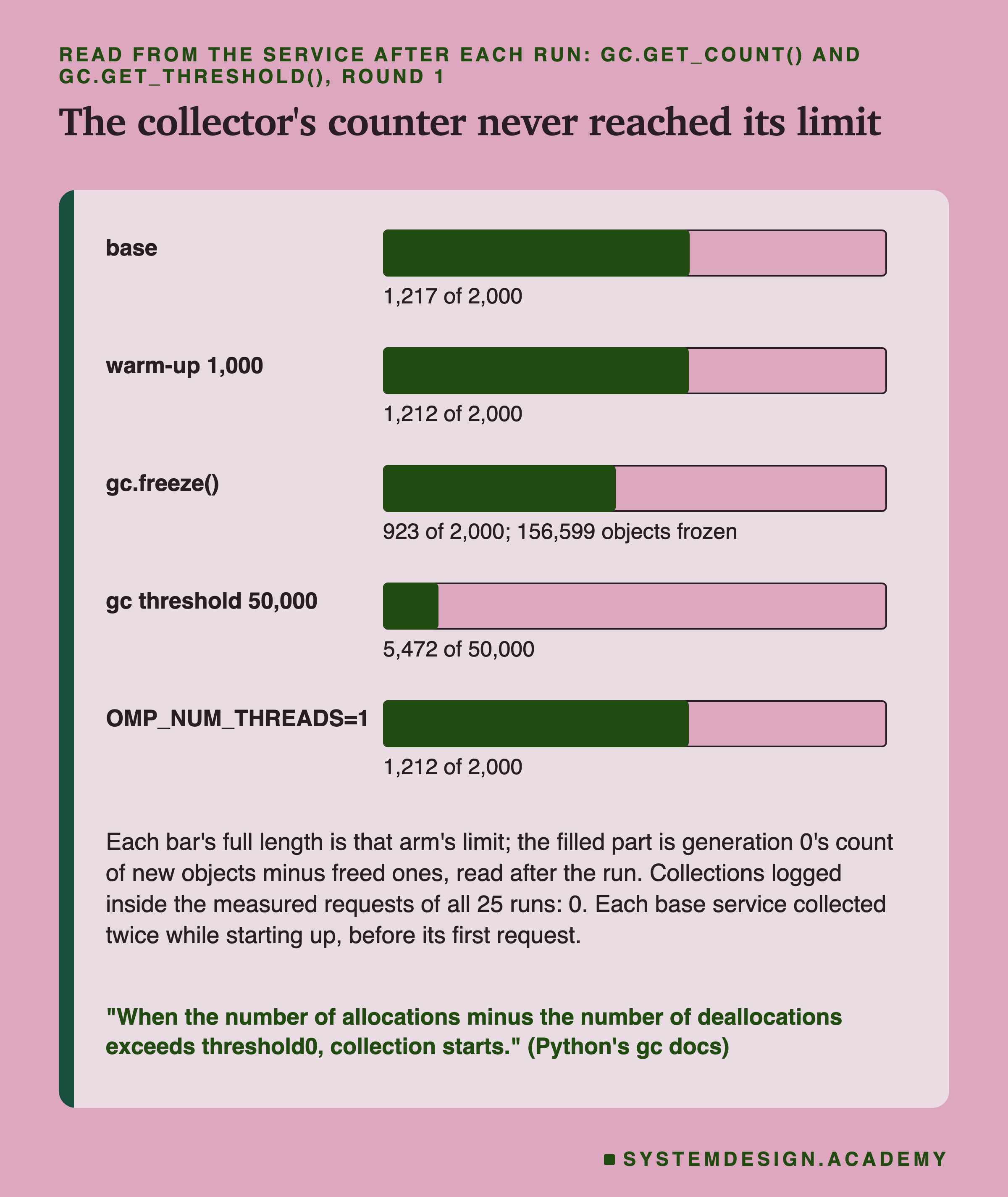
Five bars, one per arm, round 1, each bar's full length being that arm's limit for starting a collection, and the filled part the count read after the run. Base: 1,217 of 2,000. Warm-up 1,000: 1,212 of 2,000. gc.freeze(): 923 of 2,000; 156,599 objects frozen. gc threshold 50,000: 5,472 of 50,000. OMP_NUM_THREADS=1: 1,212 of 2,000. Below: each bar's full length is that arm's limit; the filled part is generation 0's count of new objects minus freed ones, read after the run; collections logged inside the measured requests of all 25 runs: 0; each base service collected twice while starting up, before its first request. Caption, a quote from Python's gc docs: "When the number of allocations minus the number of deallocations exceeds threshold0, collection starts."

The hook worked. In every base run it logged two generation-0 collections while the service was starting, about 0.7 seconds before the first request. Python's own counters, read after the run, agree. The arm with the raised limit, which made no such collections at start-up, shows two fewer generation-0 collections in Python's totals.

Why none after that? Python's documentation says: "When the number of allocations minus the number of deallocations exceeds threshold0, collection starts." The limit, threshold0, was 2,000 on this Python. Each request makes some new objects, such as the parsed body, the row and the answer. But almost all of them are freed again before the next request, the moment nothing uses them. So the count of "new minus freed" barely moves. After 100,000 requests it stood at 1,217, under 2,000, and it was the same in all five base runs.

What that means for the two garbage-collector changes. gc.freeze() froze 156,599 objects, and the raised limit put the line at 50,000 instead of 2,000. But there were no collections to remove or delay, so neither change had anything to work on here. This is a fact about this handler on this Python, not about Python services in general. A handler that keeps objects alive between requests, for example in a growing cache, would push the count up, and then the collector would run.

In a Slow Request, Every Step Was Slower

If not the garbage collector, then what? This slide and the next three are what I found when I looked harder. The comparisons use numbers the design asked for; reading them as one story about bursts came after the results, and I label it that way.
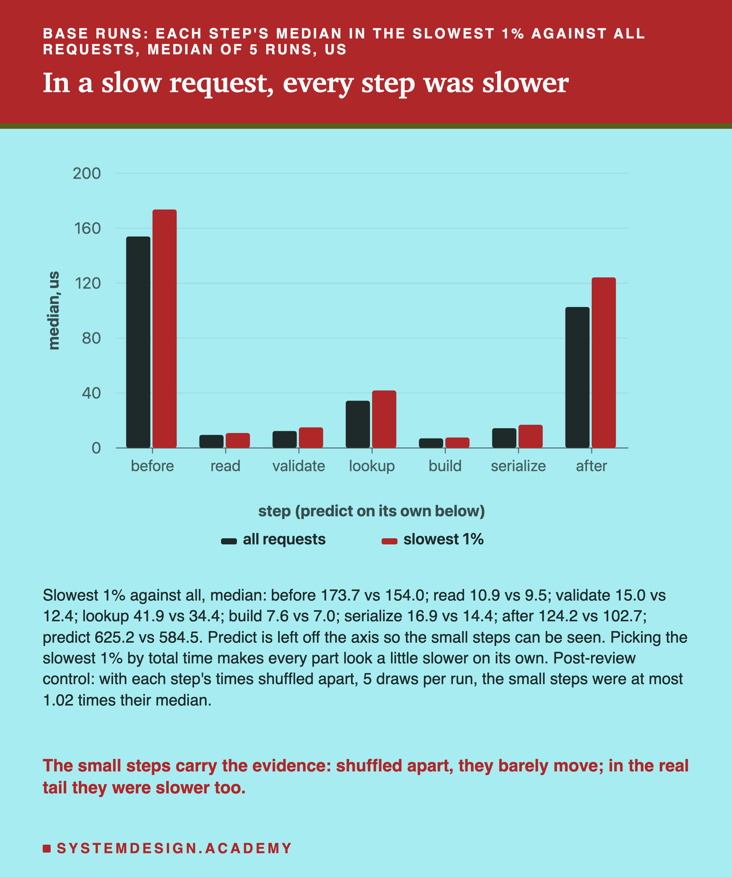
A grouped bar chart of the median time of seven steps in microseconds, for all requests and for the slowest 1%, median of 5 base runs: before 154.0 against 173.7; read 9.5 against 10.9; validate 12.4 against 15.0; lookup 34.4 against 41.9; build 7.0 against 7.6; serialize 14.4 against 16.9; after 102.7 against 124.2. Predict is left off the axis so the small steps can be seen: 584.5 against 625.2. Below that: picking the slowest 1% by total time makes every part look a little slower on its own; post-review control, with each step's times shuffled apart, 5 draws per run, the small steps were at most 1.02 times their median. Caption: the small steps carry the evidence; shuffled apart, they barely move; in the real tail they were slower too.

Look at each step on its own. In the tail, every step was slower than its usual median. Predict took 625.2 microseconds against 584.5, the work before the handler 173.7 against 154.0, and after it 124.2 against 102.7. Even building the six-number row took 7.6 against 7.0. Every step's tail median was between 1.07 and 1.22 times its usual median.

Part of this is a trap. Suppose you pick the slowest 1% of requests by their total time. Then every part of them looks a little slower, even if the parts have nothing to do with each other. A request is more likely to make the top 1% when any of its parts happens to be slow. So, after the independent review of this lesson, I added a labelled control. I shuffled each step's column of times on its own, so the steps of one request no longer belong together. Then I took the top 1% of the new totals. I did that 5 times per run.

In the shuffled data, the small steps barely moved. Read, validate, lookup, build and serialize were at most 1.02 times their usual median in the shuffled tail. In the real tail they were 1.05 to 1.26 times. That is the clue, and it holds in every run. The big steps are partly the trap. In the shuffled tail, the time before the handler was already 1.04 to 1.10 times its median. Predict was 1.03 to 1.05, and the time after the handler 1.08 to 1.13. The real values were higher in every run, but in run 5 only just (the smallest margin was 0.002, for the time before the handler).

So the small steps carry the evidence: they were slower together in the real tail, not because of how I picked it. If one thing in my code were slow, such as the database, one step would stand out and the rest would look normal. Instead, even tiny steps that do almost nothing ran slower at once, as if the whole core had slowed down for a while.

The Slowest Request Was Always the First

Now the very slowest request of each run.
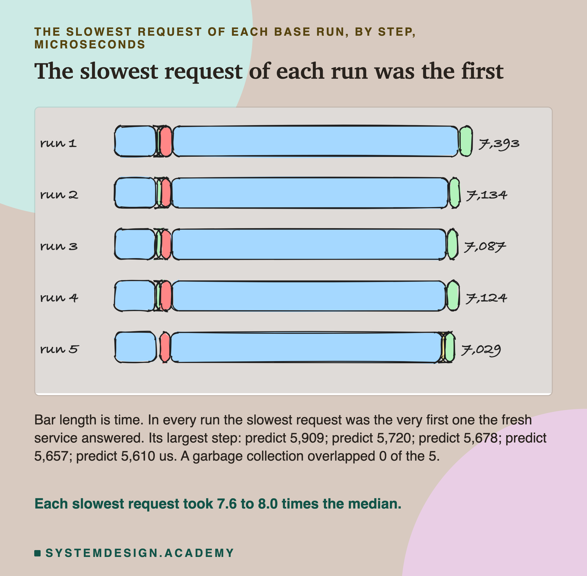
A hand-drawn chart with one long bar per base run, each split into the steps of the slowest request, labelled with its round trip in us: run 1, 7,393; run 2, 7,134; run 3, 7,087; run 4, 7,124; run 5, 7,029. In each bar the predict step fills most of the length. Below: bar length is time; in every run the slowest request was the very first one the fresh service answered; its largest step, predict 5,909, 5,720, 5,678, 5,657 and 5,610 us; a garbage collection overlapped 0 of the 5. Caption: each slowest request took 7.6 to 8.0 times the median.

In all five runs, the slowest request was request number 1, the first one the fresh service answered. It took 7,029 to 7,393 microseconds, and its predict step alone took 5,610 to 5,909, about ten times a normal predict.

Lesson 2 saw the same thing in its warm-up: its first request took more than four times a normal one. The first call to a fresh program pays for things that later calls find ready, such as code and data being read into memory for the first time. Lesson 6, cold start, measures that cost properly. Here, the point is simpler: with no warm-up, the max of a run is just the first request.

Which Step Made Each Slow Request Slow

For each tail request, the lab found the step that was furthest over its own usual time, in microseconds.
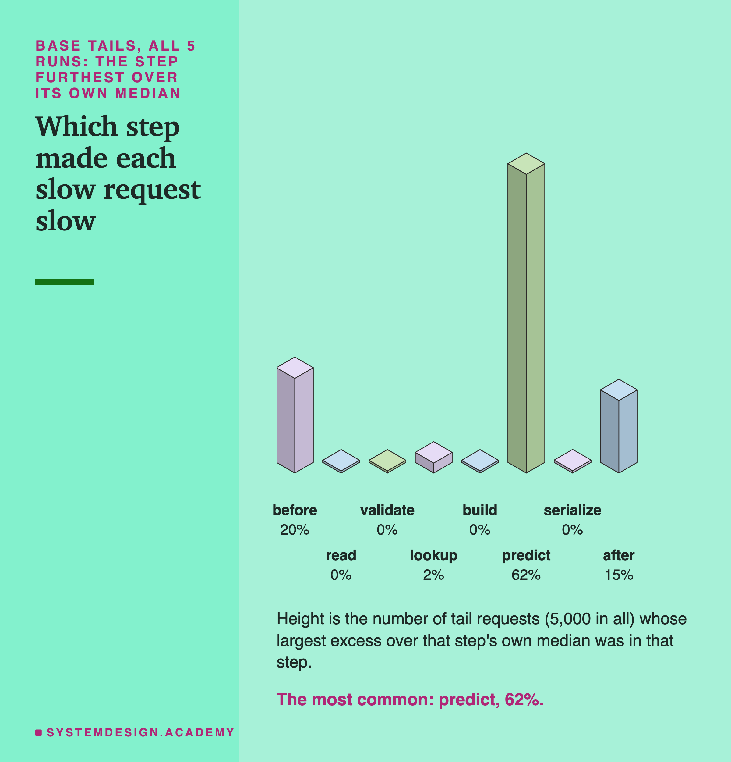
An isometric drawing of eight towers, one per step, each as tall as the number of tail requests whose largest excess over that step's own median was in that step, all 5 base runs, 5,000 tail requests: before 20%, read 0%, validate 0%, lookup 2%, build 0%, predict 62%, serialize 0%, after 15%. Caption: the most common, predict, 62%.

Predict was the step furthest over its own median in 62% of tail requests, the time before the handler in 20%, and after it in 15%. The lookup came to 2%.

Do not read this as "predict causes the tail". Predict is by far the longest step, about 585 of the 924 microseconds. If every step slows down by the same share, the longest step gains the most microseconds and wins this count. The previous slide showed that is what happened: all steps slowed together. This chart says where the extra microseconds landed, not what caused them. I keep it because it is the question the design asked, and because the honest answer to it is "mostly predict, for a boring reason".

Slow Requests Came in Bursts

Were the tail requests spread evenly through a run, or bunched together? The design asked for this, as "time".
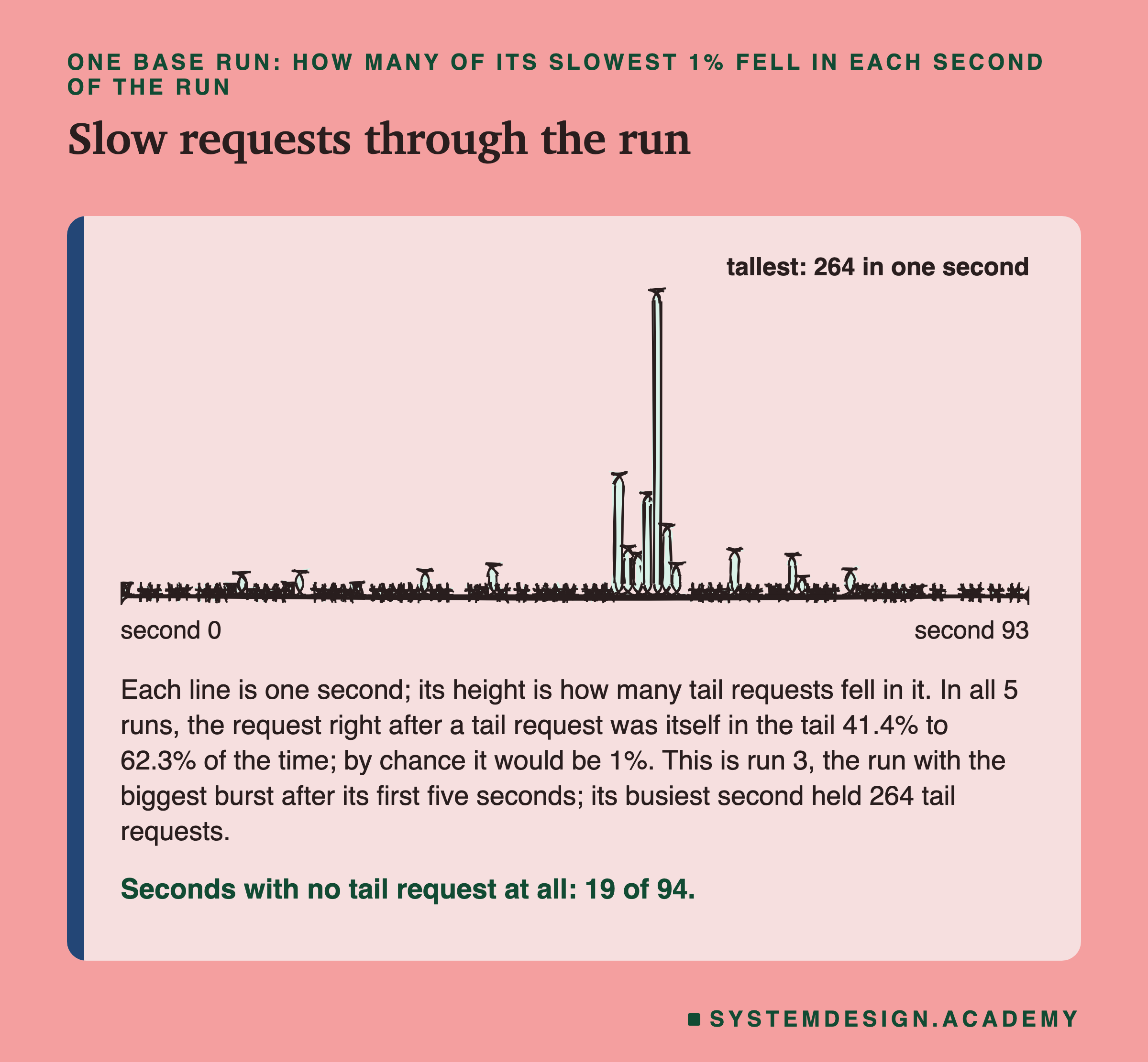
A hand-drawn strip of one base run, run 3, with one thin bar per second for 94 seconds, each as tall as the number of its slowest-1% requests that fell in that second. Most seconds have very few; a group of tall bars stands around the middle of the run, the tallest labelled 264 in one second. Below: each line is one second; its height is how many tail requests fell in it; in all 5 runs the request right after a tail request was itself in the tail 41.4% to 62.3% of the time, by chance it would be 1%; this is run 3, the run with the biggest burst after its first five seconds; its busiest second held 264 tail requests. Caption: seconds with no tail request at all, 19 of 94.

Bunched. If slow requests came at random, the request right after a slow one would be slow 1% of the time, like any other. In the five runs it was slow 41.4% to 62.3% of the time. A slow request was a sign that the next one would be slow too.

You can see it in the strip. A run lasted about 93 seconds, about 1,080 requests per second. In run 3, one second held 264 of the run's 1,000 tail requests, while 19 seconds held none at all. The busiest second in each run held 70 to 264 tail requests.

My reading, after the results: put this together with the previous slides. For a few seconds at a time, the whole core ran more slowly, every step together, and then went back to normal. I logged the load, the CPU counters and the system log, and none of them shows what caused those seconds. Run 5 had no second without a tail request and its busiest second held only 70, so its slow requests were more spread out. So the bursts vary from run to run as well.

Did Slowness Follow the Customer?

Every run asked the same customers in the same order, so the same position in two runs is the same customer and date. Did the same requests land in the tail each time?
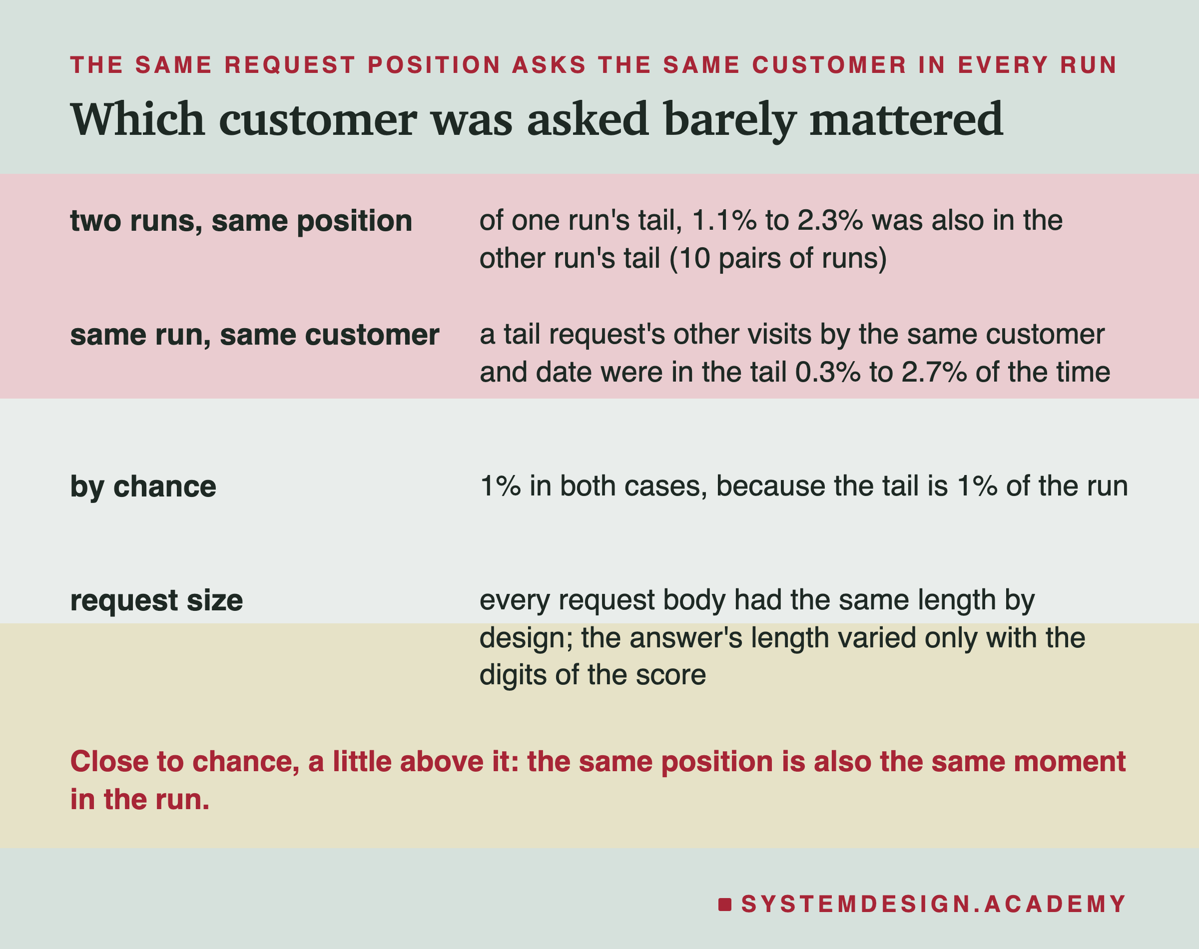
Four rows. Two runs, same position: of one run's tail, 1.1% to 2.3% was also in the other run's tail, 10 pairs of runs. Same run, same customer: a tail request's other visits by the same customer and date were in the tail 0.3% to 2.7% of the time. By chance: 1% in both cases, because the tail is 1% of the run. Request size: every request body had the same length by design; the answer's length varied only with the digits of the score. Caption: close to chance, a little above it; the same position is also the same moment in the run.

Hardly. Between two runs, 1.1% to 2.3% of one run's tail sat at the same positions as the other run's tail. Chance would give 1%. Inside one run, when a customer was asked again later, that later visit was in the tail 0.3% to 2.7% of the time.

The pairs of runs are a little above chance. One possible reason has nothing to do with the customer. The same position is also the same moment in the run, such as the first seconds, so anything tied to time also lines up. I did not separate the two.

Request size could not matter by design: every request body had the same length, because the request ids were all seven digits. So this lab cannot say whether bigger requests are slower. A real service with very different request sizes should check that.

One Change at a Time, Against the Same Base

Now the four changes. For each arm and each round, I subtracted base's number from the arm's number in the same round. That gives five differences per arm.

The rule, written before the runs: a change is "told apart from run-to-run noise" only if two things hold. All five differences have the same sign, AND the arm's five values and base's five values do not overlap at all. Otherwise, it "cannot be told apart from run-to-run noise".
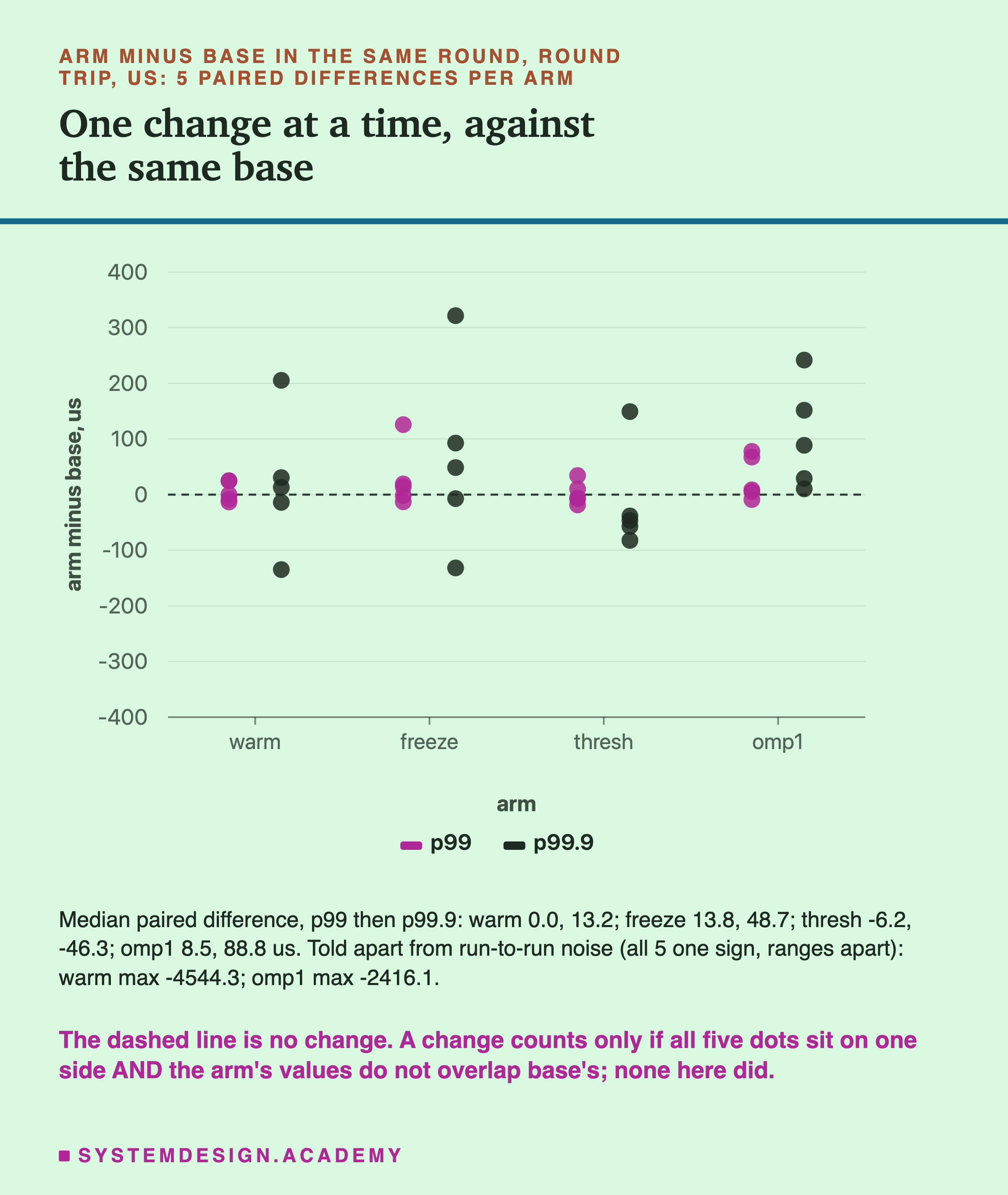
A dot chart of arm minus base in the same round, round trip, in microseconds, for four arms: warm, freeze, thresh and omp1, with five p99 dots and five p99.9 dots each, and a dashed line at zero. The dots of every arm fall on both sides of the line or touch it, except omp1's p99.9 dots, which are all above it. Below: median paired difference, p99 then p99.9: warm 0.0, 13.2; freeze 13.8, 48.7; thresh -6.2, -46.3; omp1 8.5, 88.8 us; told apart from run-to-run noise, all 5 one sign and ranges apart: warm max -4544.3; omp1 max -2416.1. Caption: the dashed line is no change; a change counts only if all five dots sit on one side and the arm's values do not overlap base's; none here did.

The warm-up lowered the max: told apart. The median difference was 4,544.3 microseconds lower, and all five rounds agreed. Of course it did: the max was the first request, and the warm-up sends that request before the counting starts. The warm arm's max was still 2,170 to 2,849 microseconds. In each run it was one request in the middle of the run, at positions 20,847 to 99,520. It had one or two steps far over their usual time, and it was not the first request. Its p99 could not be told apart from base (a median difference of 0.0), and neither could its p99.9.

gc.freeze() and the raised threshold: cannot be told apart from run-to-run noise on any of the six numbers. The raised limit's p99.9 was 46.3 microseconds lower at the median, but the five differences ran from -82.2 to +149.2. With no collections to remove, I expected nothing here, and nothing could be measured.

OMP_NUM_THREADS=1 lowered the max: told apart. That surprised me, and it gets its own slide. Its p99.9 was higher than base's in all five rounds. For the round trip it was higher by 10.5 to 241.8 microseconds, and for the handler's work by 3.9 to 114.9. But the arm's and base's values overlapped, so by my rule neither can be told apart from run-to-run noise. Five out of five in one direction is worth a second look on another box.

What OMP_NUM_THREADS=1 Means on One Core

OpenMP is a library that lets a program split work across several threads, one per core. scikit-learn uses it inside the model's predict. OMP_NUM_THREADS is a setting that tells OpenMP how many threads it may use. scikit-learn's documentation says that by default, its OpenMP code "will use as many threads as possible, i.e. as many threads as logical cores".

On this box there is one logical core. So the default is already one thread, and the box confirmed it: with the setting unset, scikit-learn reported 1 thread. Setting it to 1 should change nothing in the steady state, and that is what I saw: the p50 and p99 could not be told apart from base.

But the first request changed. With the setting unset, the first request took 7,029 to 7,393 microseconds across the runs; with OMP_NUM_THREADS=1, 4,654 to 4,788. The max fell by 2,301.1 to 2,738.7 microseconds in every round.

One possible reason is that, without the setting, the OpenMP library does extra work on its first use to decide how many threads to start. The setting may let it skip that. I did not test this, so it stays a guess. What I can say is measured. On this box, setting OMP_NUM_THREADS=1 made the first request about 2.4 milliseconds cheaper, and a warm-up removed the first request from the count altogether.

On a machine with many cores the setting matters much more, because there the default is many threads. Lesson 5, workers and threads, measures that.

A Page That Needs Ten Answers

Now the bus question from the first slide. Suppose one page needs ten answers from the model, asked one after another. The page is as slow as its slowest answer. How often does at least one of the ten land in the tail?
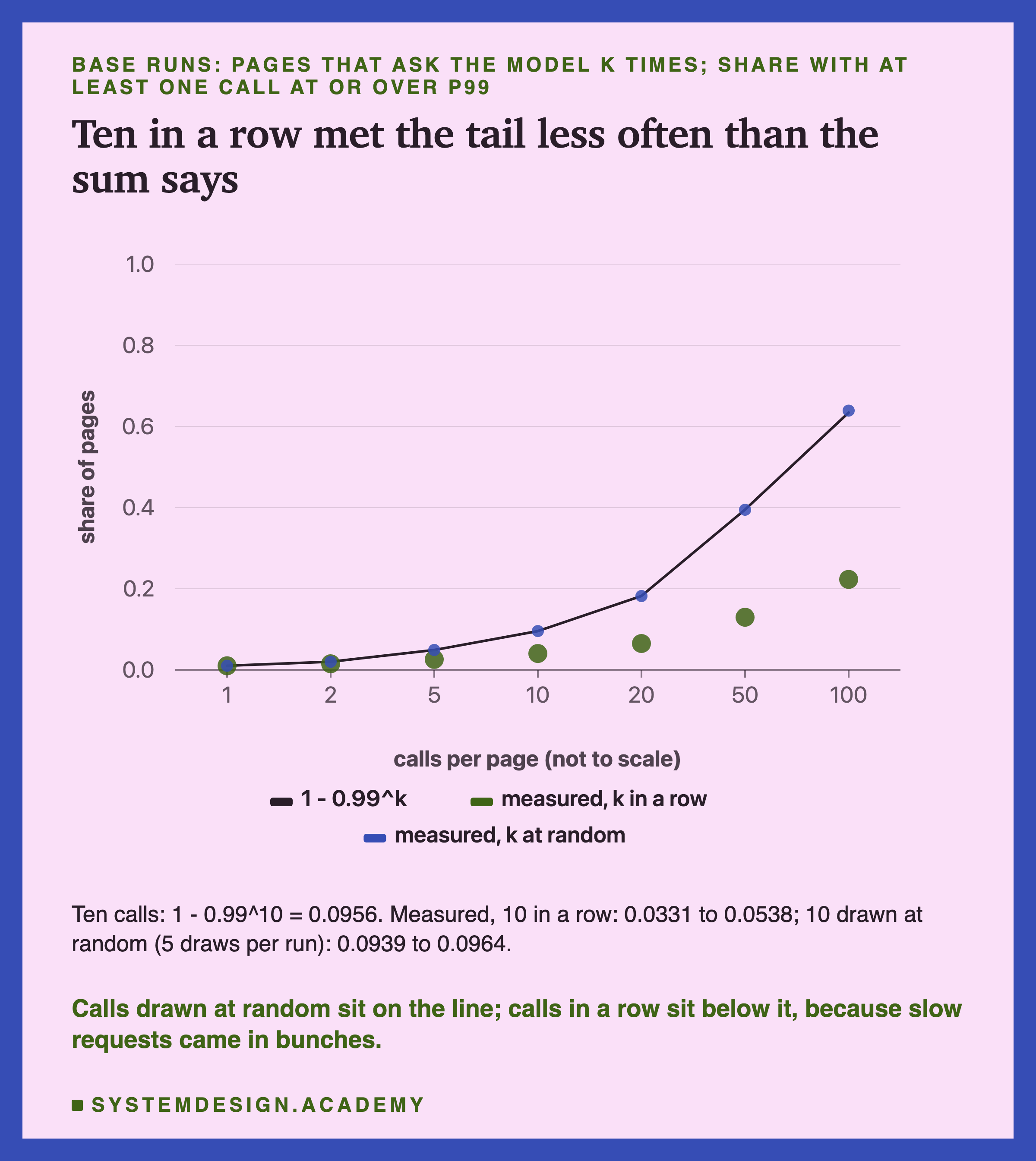
A chart of the share of pages with at least one call at or over p99 against the number of calls per page, 1, 2, 5, 10, 20, 50 and 100, not to scale. A line shows 1 - 0.99^k rising from 0.01 to about 0.63. Small dots for k calls drawn at random sit on the line. Larger dots for k calls in a row sit below it, at about 0.22 for 100 calls. Below: ten calls, 1 - 0.99^10 = 0.0956; measured, 10 in a row, 0.0331 to 0.0538; 10 drawn at random, 5 draws per run, 0.0939 to 0.0964. Caption: calls drawn at random sit on the line; calls in a row sit below it, because slow requests came in bunches.

The textbook answer. Suppose each call is in the tail with chance 1 in 100, and the calls are independent. Then all ten are fast with chance 0.99 multiplied by itself ten times, 0.9044. So at least one is slow with chance 1 - 0.99^10 = 0.0956, almost one page in ten. Independent means the luck of one call tells you nothing about the next.

What the lab measured. I cut each base run into 10,000 pages of 10 calls in a row. Only 3.3% to 5.4% of them had a call in the tail, about half of 9.56%. As a check of my arithmetic, not a finding, I also made pages from 10 calls picked at random from the whole run, five times per run. Picking at random makes the calls independent by construction, so these pages must land on the formula, and they did: 9.39% to 9.64%. That tells me the page counting is right. It says nothing about real pages.

Why the difference? The calls of a real page come one after another, and here slow calls came in bunches. When a slow second arrives, many of its slow calls fall into the same few pages. So fewer pages get hit, but the pages that are hit often get several slow calls. The evidence that the calls in a row were not independent is on the bursts slide. The request after a slow one was slow too 41.4% to 62.3% of the time, against 1% by chance. The formula assumes independence, so it overstates how many pages are hit here.

At 100 calls in a row, 16.2% to 33.6% of pages met the tail, against 63.4% for independent calls.

Why the Textbook Number Is Still Worth Knowing

The measured pages were luckier than the formula. Should you forget the formula then? No.
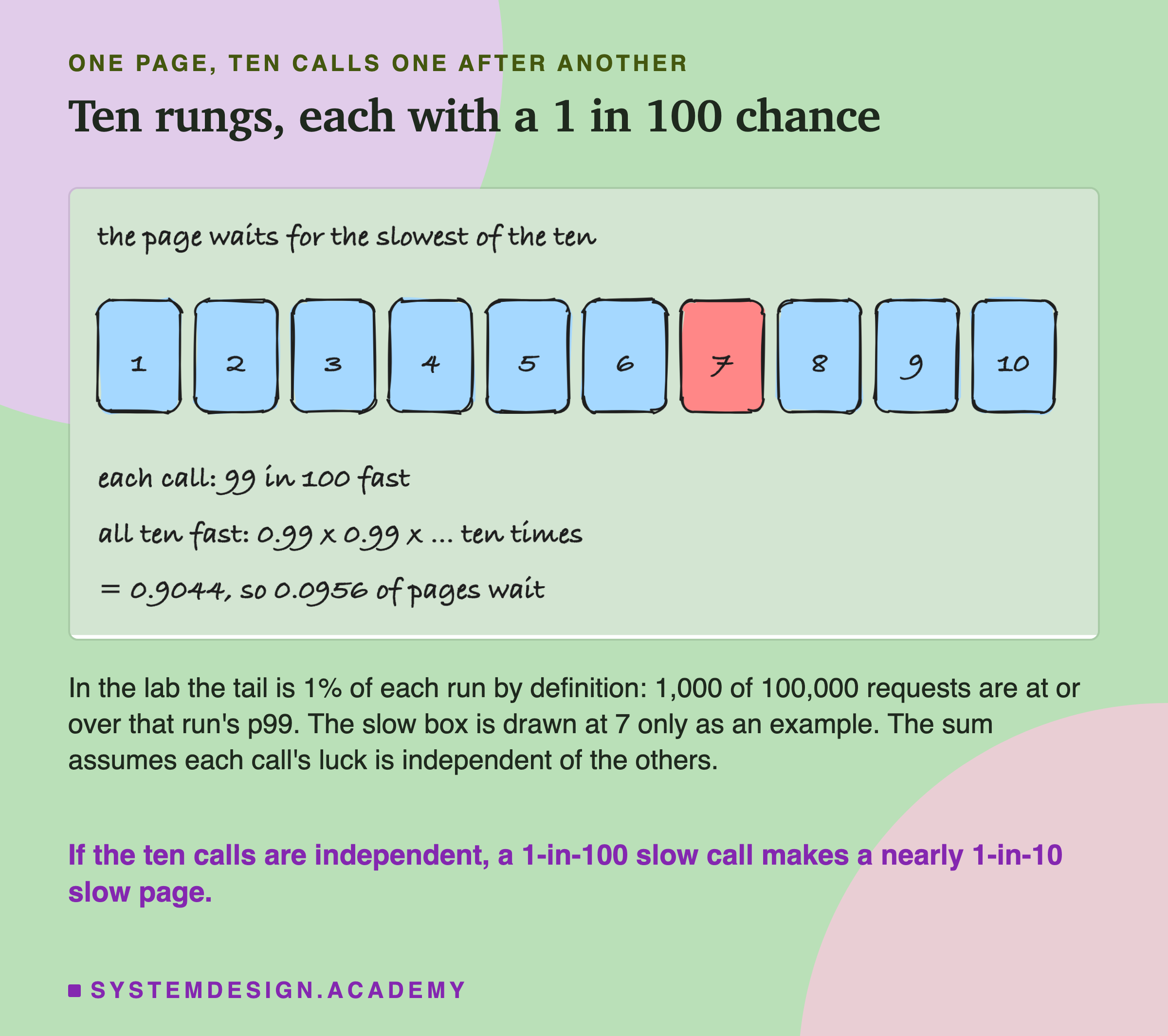
A hand-drawn row of ten numbered boxes for ten calls, one after another, box 7 marked as the slow one; the page waits for the slowest of the ten. Below the boxes, in handwriting: each call, 99 in 100 fast; all ten fast, 0.99 x 0.99 x ... ten times, = 0.9044, so 0.0956 of pages wait. Below: in the lab the tail is 1% of each run by definition, 1,000 of 100,000 requests are at or over that run's p99; the slow box is drawn at 7 only as an example; the sum assumes each call's luck is independent of the others. Caption: if the ten calls are independent, a 1-in-100 slow call makes a nearly 1-in-10 slow page.

The formula is the right first guess when calls are independent. That holds more often in a real system than on my one box. Ten calls might go to ten different machines, each with its own bad moments, or they might run at the same time instead of one after another. Then one machine's slow second does not bunch the slow calls together, and the textbook number is close.

The lesson from my data is narrower. Bunching changes the answer in both directions. Fewer pages are hit, but a hit page can be hit many times. So measure the page itself, not only the call. Here, even 100 calls in a row met the tail in only 16% to 34% of pages, against 63% for the formula. And notice how fast the formula grows. One slow call in 100 gives about one slow page in 10 at 10 calls, and almost two in 3 at 100 calls. A page that makes many calls lives in its calls' tail.

The design also checked the p99.9 for pages of 10. The formula gives 0.0100. Ten calls in a row hit the deep tail 0.35% to 0.47% of the time, and calls drawn at random hit it 0.98% to 1.00%. The same bunching shows there too.

My Seven Guesses Before the Run, Checked

I wrote seven guesses into the lab before it ran. Some guesses had several parts, so the report checks thirteen statements. Five were right and eight were wrong.

  1. "Base round trip: p99 under 1.5x the median; p99.9 at least 2x the median; max at least 10x the median." First part right (1.08 times). Second wrong (1.23 times). Third wrong (7.7 times).

  2. "More than half of the base tail (round trip at or above p99) had a service collection inside its round trip (gc_in or gc_out)." Wrong, and the most wrong: none did.

  3. "The first 1,000 requests are at least 5x over-represented in the base tail (at least 5% of the tail)." Wrong by the measure I used, the median of the five runs: 1.6%. Only run 1, at 20.3%, fit the guess. Pooling all five tails instead gives 260 of 5,000, which is 5.2%, just over the line. Almost all of them come from run 1, so the answer depends on how the runs are combined.

  4. Four changes. "freeze lowers the round trip p99.9 by an amount told apart from noise; thresh lowers the p99, told apart." Both wrong: neither could be told apart. "omp1 cannot be told apart from noise on any of the six metrics." Wrong: it lowered the max. "warm lowers the max, told apart, and its p99 cannot be told apart." Both parts right.

  5. "The measured share of consecutive 10-call pages with a call over p99 is within 0.02 of 1 - 0.99^10." Wrong: 0.0331 to 0.0538, against 0.0956.

  6. "Slowness does not belong to the customer: the tails of two base runs share under 3% of their requests." Right: 1.1% to 2.3%.

  7. "Every returned score equals this Mac's score to the bit or within 1e-15." Right: 2,501,970 of 2,505,000 scores were equal to the bit, and the rest differed by at most 1.1e-16.

Eight wrong statements out of thirteen is not a failure of the lab. It is the reason to write guesses down first. Without them, I would have read "the tail is the garbage collector" into any result, because I believed it before I looked.

Try It Yourself

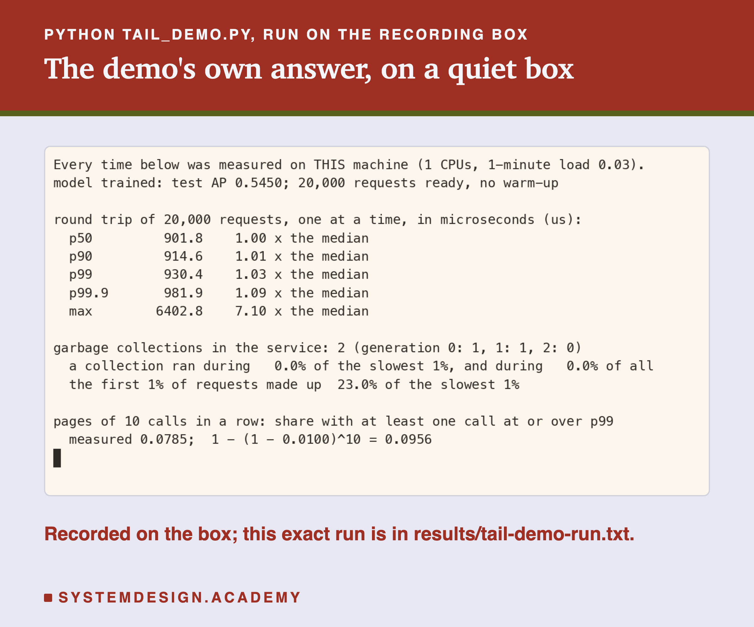
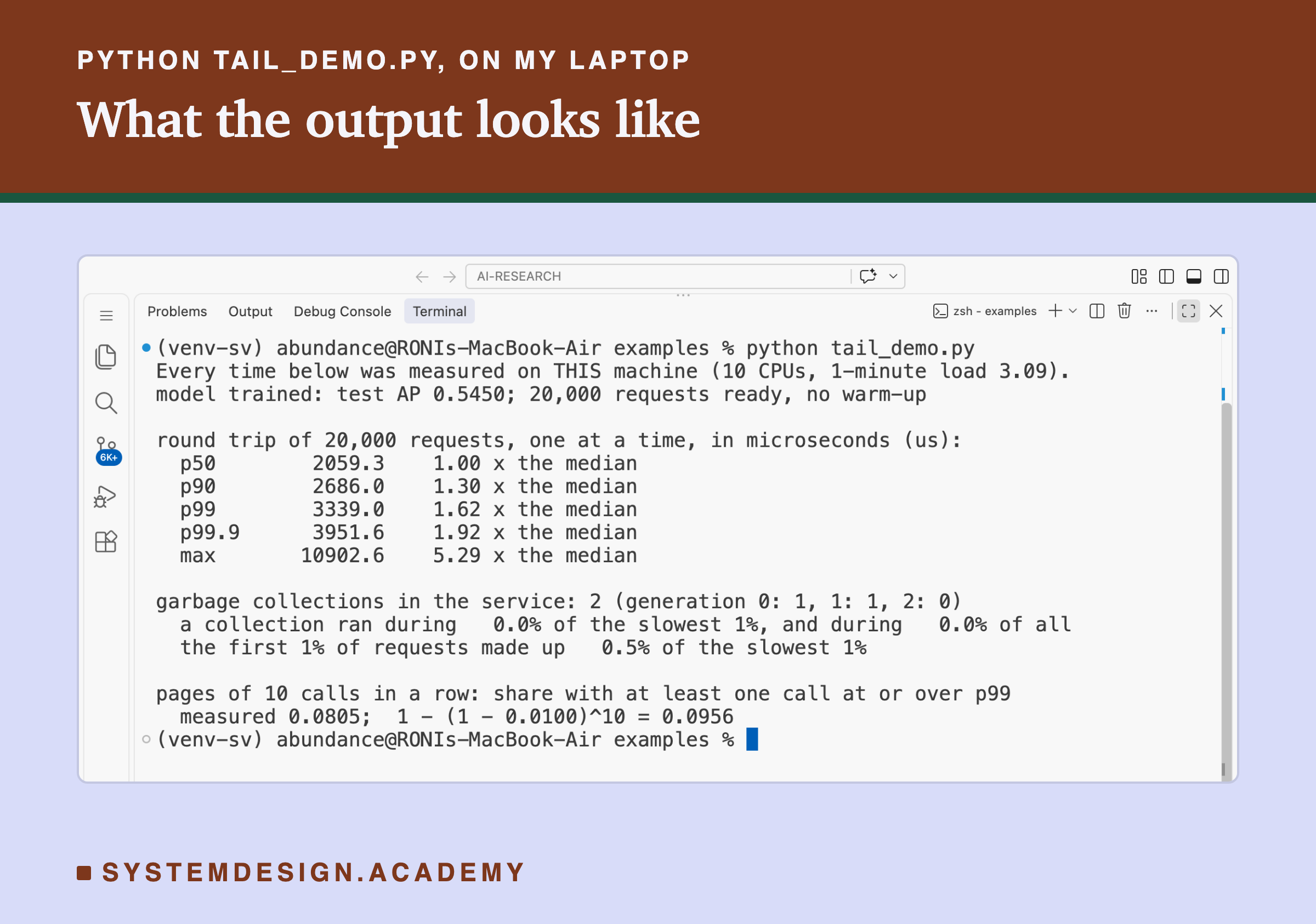
The full lab needs a rented box and about two hours. The demo, tail_demo.py, builds the same service on your own computer, sends it 20,000 requests with no warm-up, and prints the tail and what sits in it.
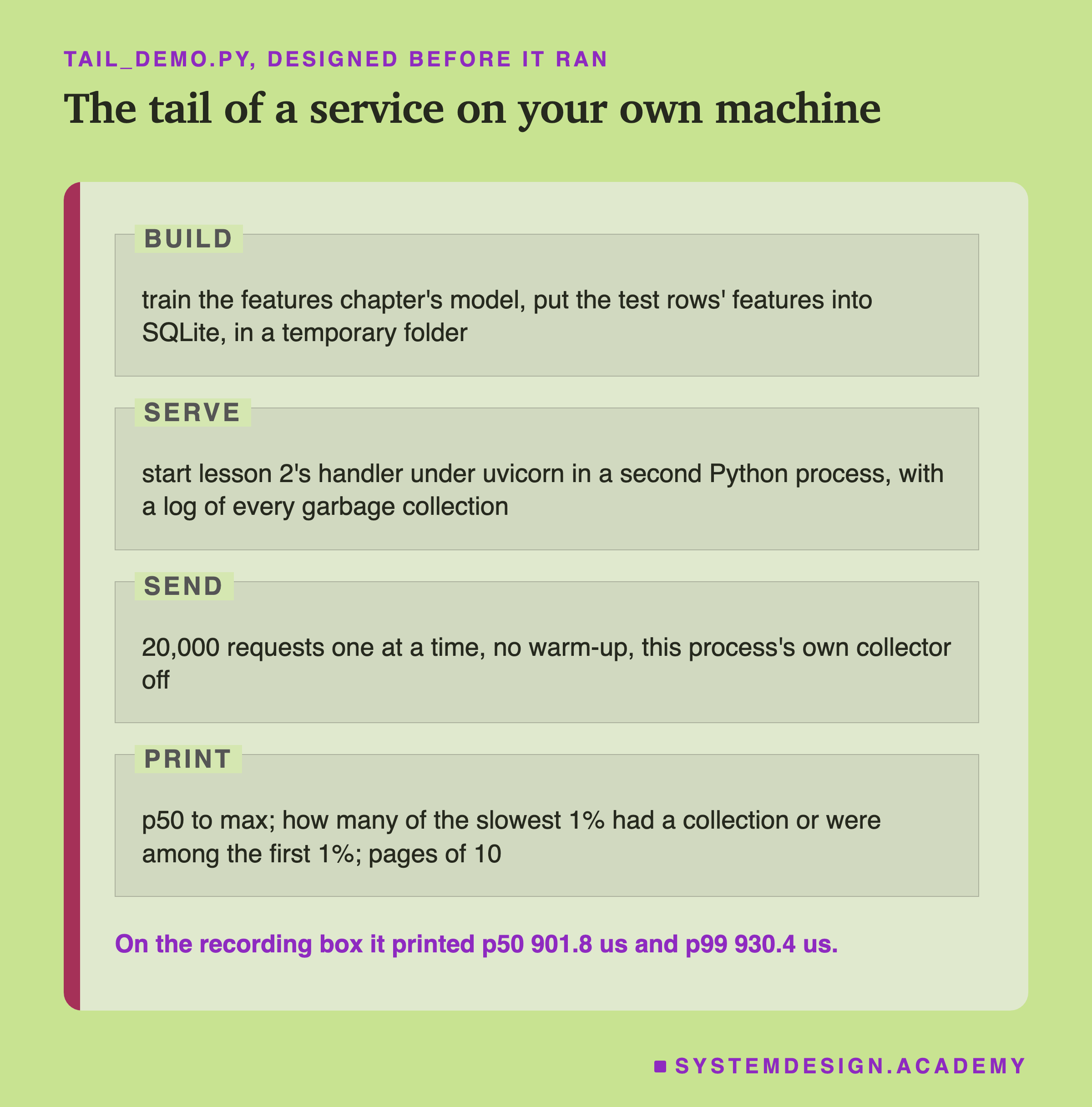
A page in four labelled zones, headed tail_demo.py, designed before it ran. Build: train the features chapter's model, put the test rows' features into SQLite, in a temporary folder. Serve: start lesson 2's handler under uvicorn in a second Python process, with a log of every garbage collection. Send: 20,000 requests one at a time, no warm-up, this process's own collector off. Print: p50 to max; how many of the slowest 1% had a collection or were among the first 1%; pages of 10. Caption: on the recording box it printed p50 901.8 us and p99 930.4 us.

I wrote the demo's design into its docstring after the lab's design and before the demo first ran. I did not change it after the results.
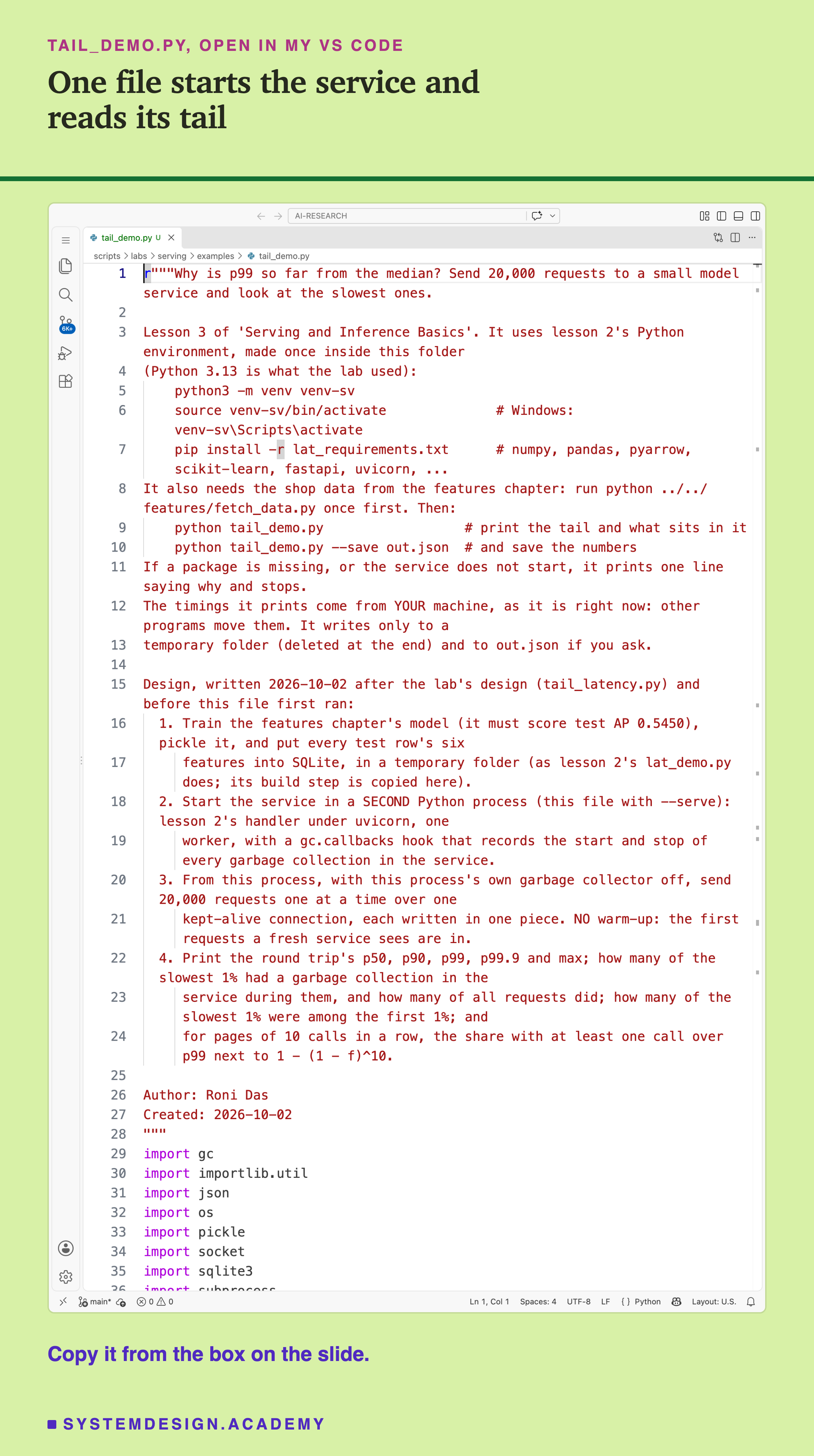
A real screenshot of VS Code with tail_demo.py open at the top of the file, showing its docstring: what it needs, how to run it, and the design written before it first ran.

Before you run this lab. The demo uses lesson 2's Python environment, with the same library versions as the lab's box. If you made it for lesson 2, use it again. If not, make it once, inside the scripts/labs/serving/examples folder:

python3 -m venv venv-sv
source venv-sv/bin/activate        # on Windows: venv-sv\Scripts\activate
pip install -r lat_requirements.txt

I used Python 3.13. Then run python ../../features/fetch_data.py once, which downloads the shop data. Now run python tail_demo.py. It needs no GPU and no cloud account. If a package is missing, or the service does not start, it prints one line saying why and stops.

The first line it prints says the times are from your machine, with its number of CPUs and its load at that moment. Read them for their shape, not for their size. How far is the max from the median? Did any collection run? Did pages of 10 meet the tail more or less often than the formula?

Pick an Arm, Pick a Run

This box holds the real round trips from the lab. It needs nothing but Python, so it runs in your browser. It has no model and no clock: it only looks up what the box measured.

Press Run. Then change ARM to "warm" and watch the max fall. Try "omp1". Change RUN to see how much one run differs from another. Set CALLS = 100 to see how the formula and the measured pages drift apart.

The report script writes this box from the lab's raw timings, runs it with six settings, and checks that each run prints the lab's numbers. The x column shows how many times the median each percentile is, so you can see the max jump in every arm without a warm-up.

The Lab's Code, Piece by Piece

The lab has one file that runs on my laptop, a few small files that run on the box, and the step script you saw above.

tail_latency.py, on my laptop, holds the design in its docstring, written before the first run. Two dated notes were added later: one when the first box's results were lost, and one when I decided to film the AWS steps. Its commands are check (lesson 2's files match by sha256), launch, provision, run, status (reads the serial console), fetch, teardown and collect. collect calls tail_stats.py, which does all the arithmetic on the raw timings and writes results/tail-result.json.

tail_files/tail_service.py is the service. It imports lesson 2's service file unchanged, so the model, the SQLite table and the handler's steps are lesson 2's. It adds three things: two readings of the thread's CPU time, the length of the body and the answer, and a gc.callbacks hook. Python calls every function in the list just before and just after each collection. So the hook can write down when each collection started and stopped, and which generation it was. The arm's setting, such as , is applied at the end of start-up.

How to Look at the Tail of Your Own Service

Here is the order I would follow, using only what this lab did.
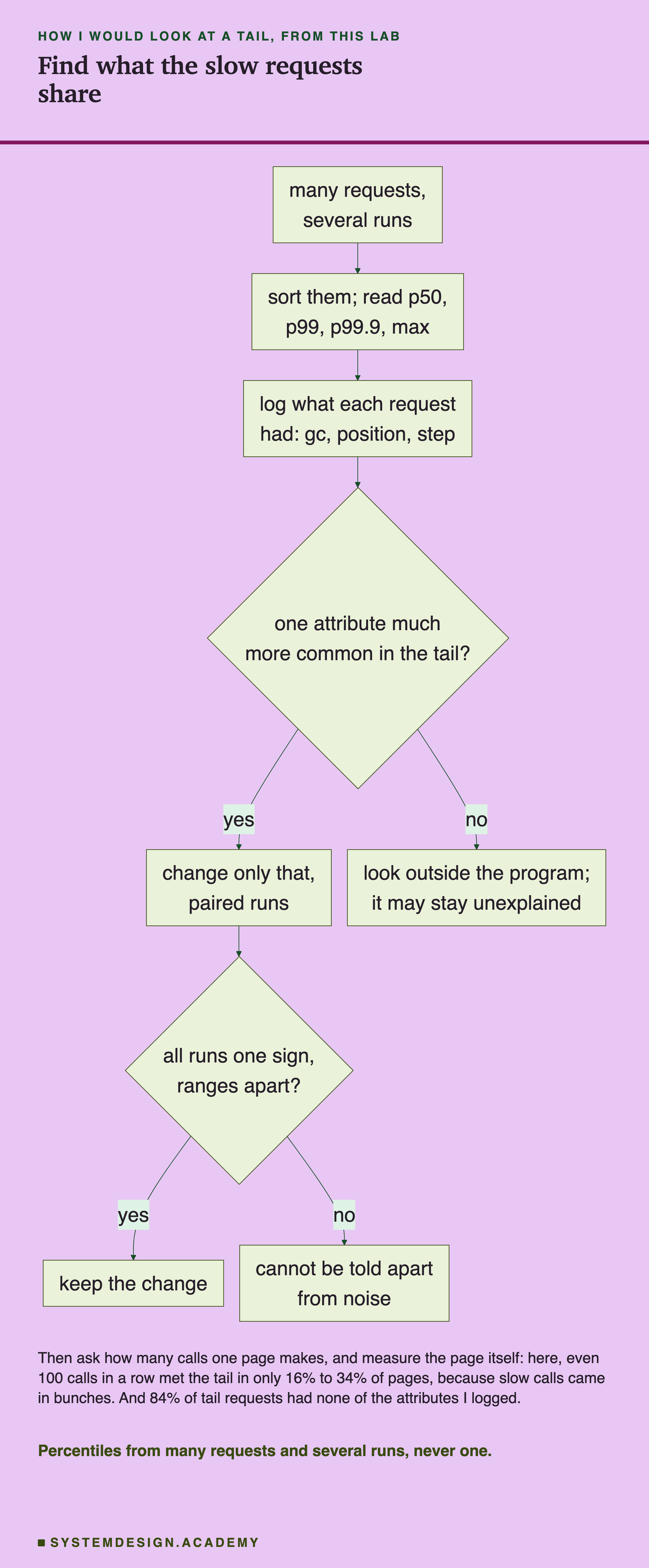
A flowchart. Many requests, several runs, leads to sort them, read p50, p99, p99.9, max, which leads to log what each request had: gc, position, step. Then a diamond: one attribute much more common in the tail? Yes leads to change only that, paired runs, then a diamond: all runs one sign, ranges apart? Yes leads to keep the change; no leads to cannot be told apart from noise. No, at the first diamond, leads to look outside the program; it may stay unexplained. Below: then ask how many calls one page makes, and measure the page itself; here, even 100 calls in a row met the tail in only 16% to 34% of pages, because slow calls came in bunches; and 84% of tail requests had none of the attributes I logged. Caption: percentiles from many requests and several runs, never one.

The chart starts where every look at a tail should start, with many requests and several runs, and works inwards. Here are the same steps in words, each with the number from this lab behind it.

  1. Send many requests, and repeat the run. Here the p99.9 of the same setup moved by about 100 microseconds from run to run. One run would have fooled me.

  2. Read the whole line, not one number. p50, p90, p99, p99.9 and max each tell you something different. Here the max was one request, the first, and nothing like the rest.

  3. Log what each request had. A gc.callbacks hook costs little and settles the garbage-collector question in a day. Here it said "never" for 500,000 requests.

  4. Compare the tail with everything. An attribute only matters if it is much more common in the tail than overall. Being off the core was about nine times more common in the tail, but it covered only one tail request in ten.

  5. Look at time. If slow requests come in bunches, fan-out behaves differently, and the cause may be outside your code. Here 84% of tail requests had none of the attributes I logged, so even a careful log may not name the cause.

When These Tricks Help, and When They Do Not

A warm-up helps when your first requests are counted or felt. Here it removed a request of about 7 milliseconds from every run. In a real service, the first user after every restart, or after every new copy of the service starts, pays that cost. Lesson 6 measures cold starts properly.

gc.freeze() helps when the collector actually runs, and runs over many long-lived objects. Python's documentation recommends it mostly for programs that start child processes with fork(). Its advice: call "gc.disable() early in the parent process, gc.freeze() right before fork(), and gc.enable() early in child processes". Here the collector did not run during requests, so there was nothing to gain. Check with a hook before you add it.

A raised threshold has a cost. Collections become rarer but bigger, and memory held by circles of objects is freed later. Here it could not be told apart from noise, because there were no collections to delay.

Do not turn the collector off to "fix" a tail you have not measured. Python's docs say you can disable it only "if you are sure your program does not create reference cycles". If you are wrong, memory grows until the process dies.

OMP_NUM_THREADS=1 is cheap to set on a one-core box, and here it made the first request faster. But its p99.9 was higher than base's in all five rounds, though not by enough to be told apart from noise. Test it on your own box before you rely on it. On a big machine it decides how many cores one predict may use, which is a real trade-off.

Do not copy my handler as it is into a busy service. Like lesson 2's, it is an async def that calls SQLite and predict_proba, which block. With one request at a time that changes nothing. Under load, a blocking call inside an async def stops every other request. FastAPI's documentation says a plain is "run in an external threadpool that is then awaited, instead of being called directly (as it would block the server)".

What This Lab Cannot Tell You
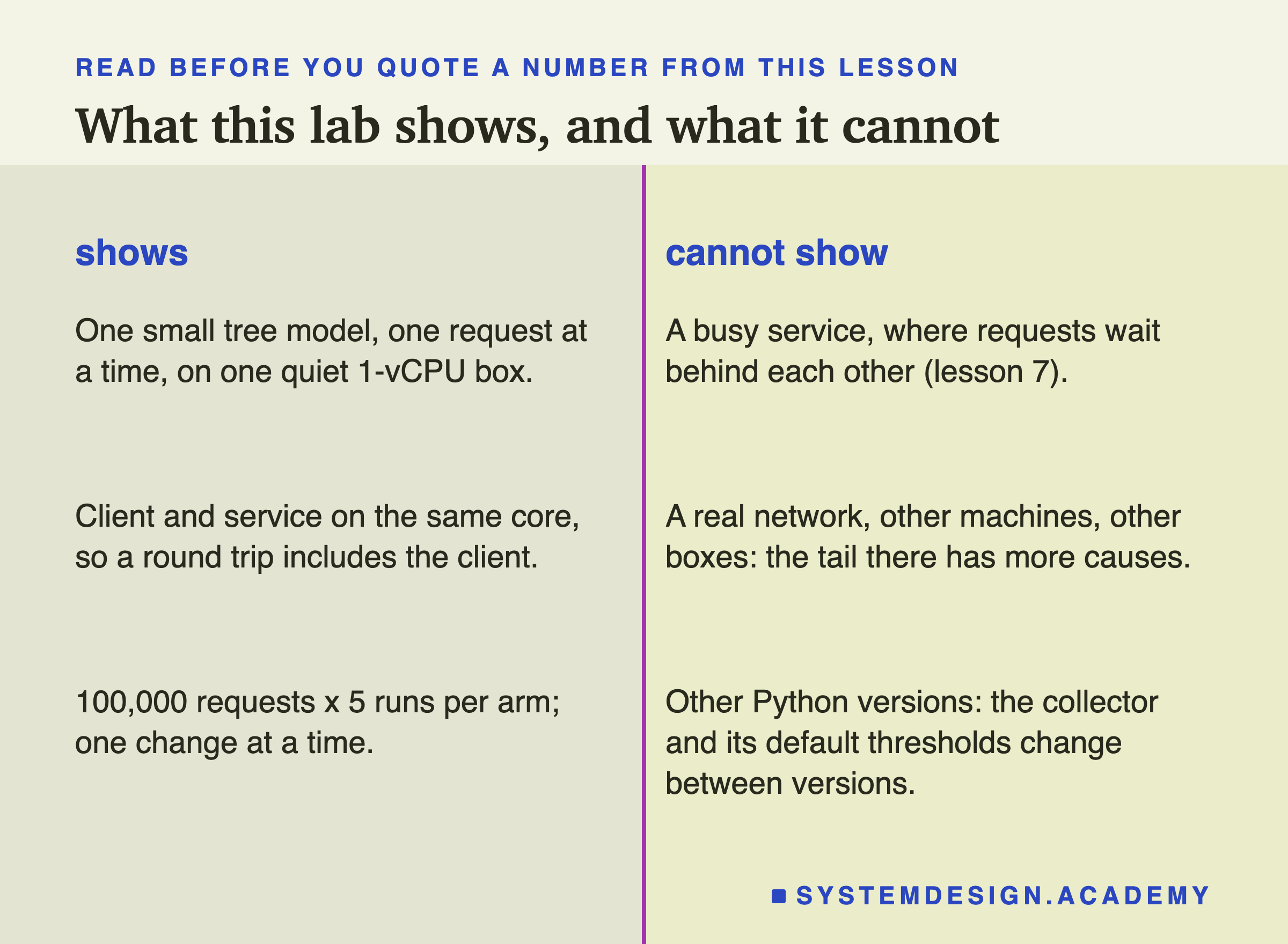
Two columns titled shows and cannot show. Shows: one small tree model, one request at a time, on one quiet 1-vCPU box; client and service on the same core, so a round trip includes the client; 100,000 requests x 5 runs per arm; one change at a time. Cannot show: a busy service, where requests wait behind each other (lesson 7); a real network, other machines, other boxes: the tail there has more causes; other Python versions: the collector and its default thresholds change between versions.

One box, one core, one request at a time. The tail of a busy service is mostly queueing: requests waiting behind other requests. None of that is here. Lesson 7 measures it.

The bursts are unexplained. I can show that for some seconds every step ran slower, and that the handler was rarely off the core, but not why. A second box of the same type might have different bursts, or none.

One Python version. On Python 3.13.15 the first collection limit is 2,000. Other versions use other numbers and, in some versions, a different collector. Check yours with gc.get_threshold().

The lost box and the recording box. The first box I rented for this lesson ran the whole schedule on 2026-10-02. It was deleted before its results were copied off, so nothing from it is used. The lab's docstring has a dated note about it. The numbers come from a second box on 2026-10-04, with the same design. The AWS recordings and the demo come from a third box, built after the second was gone. Its short schedule's timings are not used anywhere.

Labelled additions. Two changes to the report script came after the results. One fixes a crash on runs with no collections at all. The other shortens the printed lines so the recording fits the screen. Neither changes a number. The step-by-step tail comparison and the reading of the bursts are my interpretation after the results. The figure-only percentile curve was added before the second box's results were read.

After an independent review of the lesson I added three things, all labelled. The first is the shuffle control on the every-step slide. The second is a smaller lossless way of storing the raw timings; the report checks every number again from the new files. The third is a clearer version of the AWS step file, described on the build slide.

What to Do on Monday
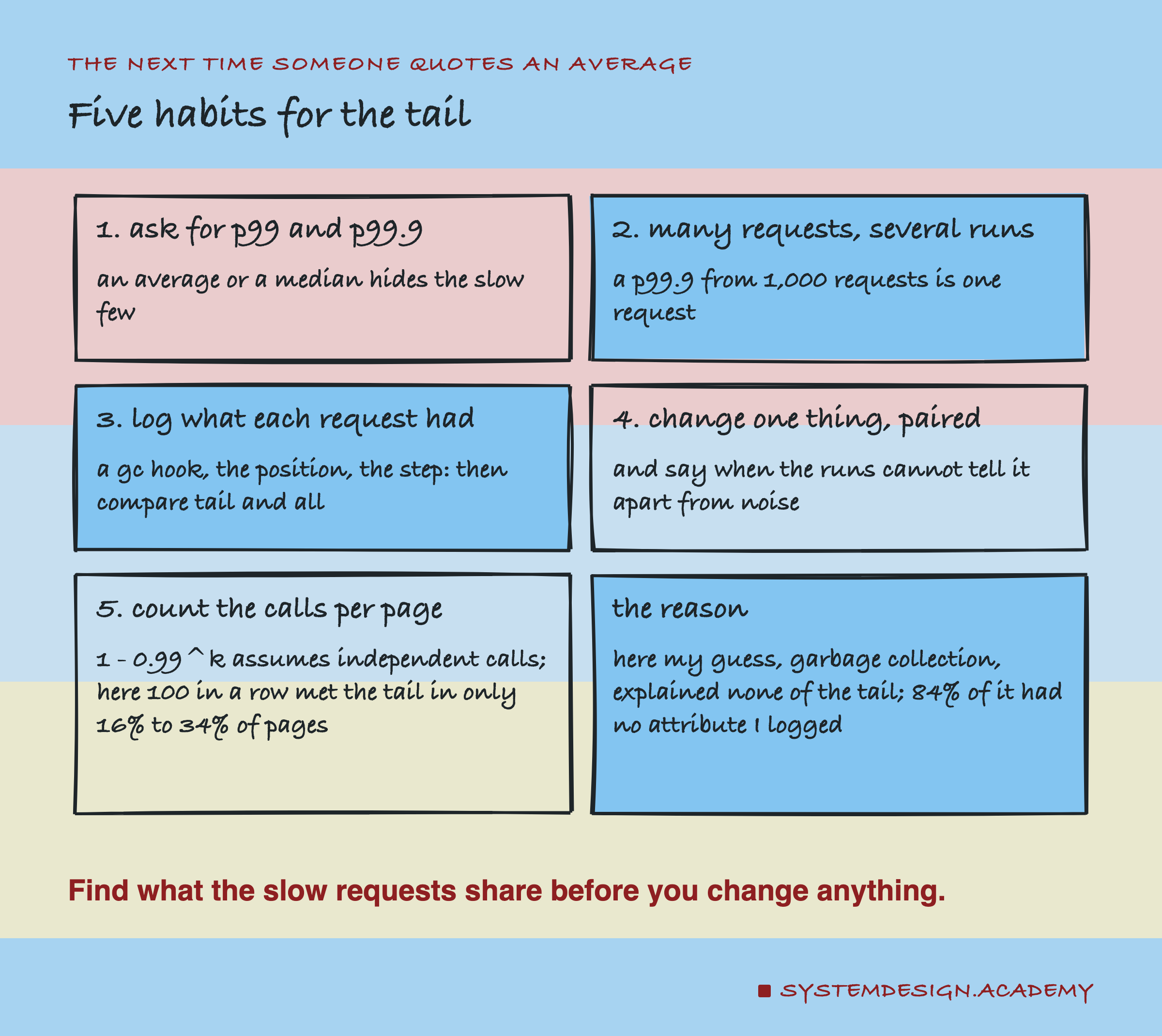
A hand-drawn grid of six cards, titled five habits for the tail. 1, ask for p99 and p99.9: an average or a median hides the slow few. 2, many requests, several runs: a p99.9 from 1,000 requests is one request. 3, log what each request had: a gc hook, the position, the step; then compare tail and all. 4, change one thing, paired: and say when the runs cannot tell it apart from noise. 5, count the calls per page: 1 - 0.99^k assumes independent calls; here 100 in a row met the tail in only 16% to 34% of pages. The reason: here my guess, garbage collection, explained none of the tail; 84% of it had no attribute I logged. Caption: find what the slow requests share before you change anything.

If you take one thing to work on Monday, add a gc.callbacks hook and a per-request log to a service you own. Then send it a few hundred thousand requests on a quiet machine, sort them, and compare the slowest 1% with everything. Do this before you change a single setting.

You may find, as I did, that your favourite suspect is innocent. And you will find out whether your service needs a warm-up after every start.
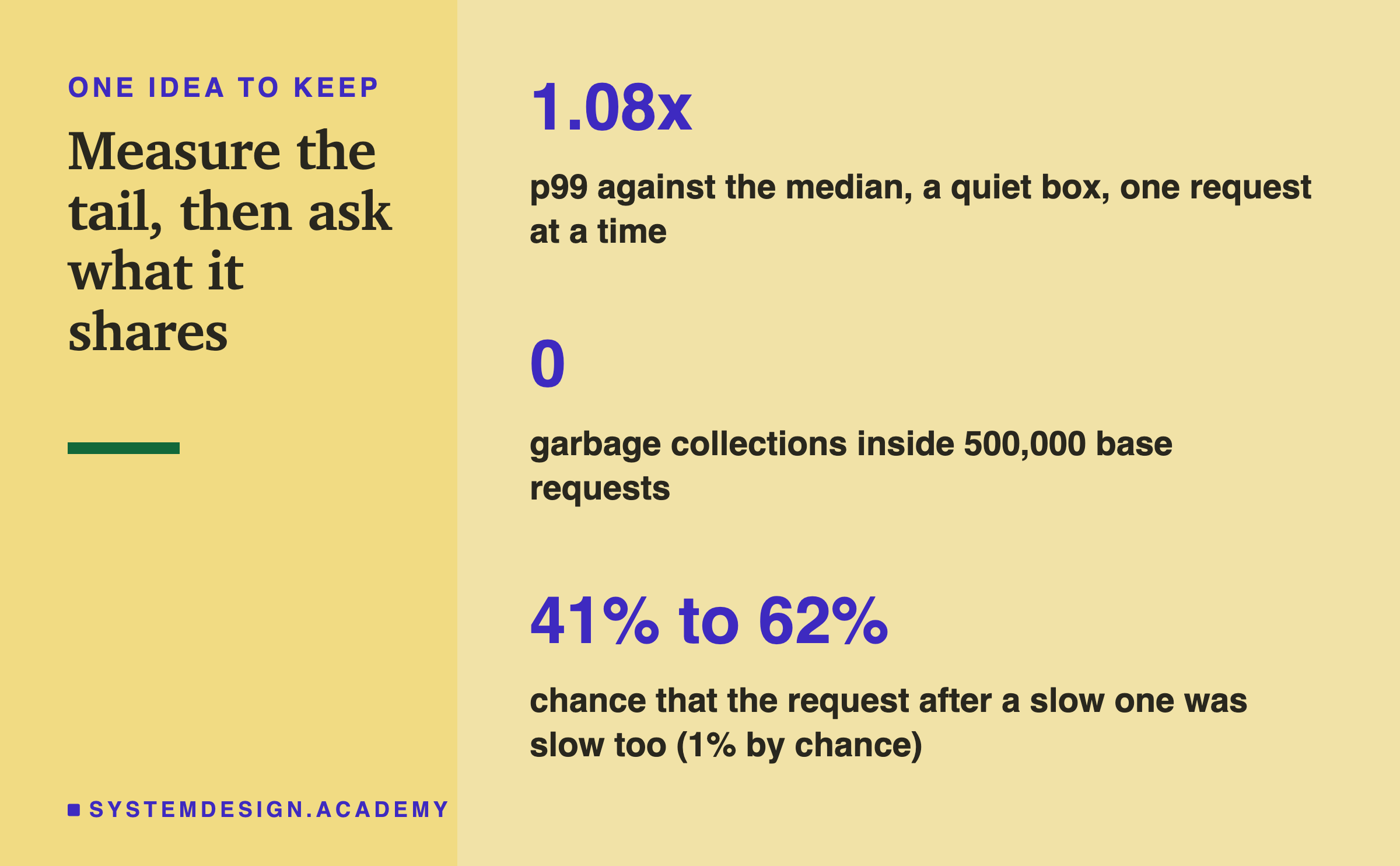
A closing card titled measure the tail, then ask what it shares. 1.08x: p99 against the median, a quiet box, one request at a time. 0: garbage collections inside 500,000 base requests. 41% to 62%: chance that the request after a slow one was slow too, 1% by chance.

The one idea to keep: the tail is made of real requests, and you can ask them what they have in common. Here the answer was not the garbage collector. It was the first request of a fresh service, and short bursts in which everything ran slower. Those bursts also made pages of ten calls luckier than the textbook formula says. Measure first, and let the slow requests tell you.

Knowledge Check

Knowledge Check

4 questions - Score 80% to pass

Q1

In the base runs, how many garbage collections ran during the measured requests?

Q2

What was the slowest request of every base run?

Q3

Pages of 10 calls in a row met the tail 3.3% to 5.4% of the time, not 9.56%. Why?

Q4

The raised gc threshold lowered the p99.9 by 46.3 microseconds at the median. What does the lesson conclude?
A warm-up is a set of requests sent first and not counted. Fan-out is when one page or one job needs many answers, so it waits for the slowest of them. Run-to-run noise is how much the same measurement moves when you simply run it again.

What I log for every request. A thread is one line of work inside a program that the operating system can run on a core. On top of lesson 2's clock readings, the handler reads its own thread's CPU time, the time the core actually spent running it. If the wall clock moved much more than the CPU time, the handler was waiting for the core. A gc.callbacks hook writes down the start, the end and the generation of every collection.

  • One request at a time. No request ever waits behind another, so queueing stays out. Lesson 7 measures queueing.

  • The round trip still includes the client and the switch between the two programs, and I label it that way everywhere.

    ssh
    scp
    rsync
    curl
    default VPC
    ~/lab-data/serving/lat/
    python latency_anatomy.py prepare
    ~/lab-data/features/retail.parquet
    python ../features/fetch_data.py

    What it costs. A c7g.medium costs $0.0363 an hour on demand in us-east-1. AWS's pricing page says you pay "by the hour or second (minimum of 60 seconds)". Two smaller charges run while the box exists. The box's public IPv4 address costs $0.005 an hour, billed "in one-second increments, with a minimum of 60 seconds". Its 16 GiB gp3 disk costs $0.08 per GB-month, also billed per second.

    The box that measured this lesson's numbers was on for 1.783 hours: $0.0647 for compute, $0.0089 for the address and $0.0032 for the disk. The recording box was on for 0.152 hours, and the first box, whose results were lost, for 3.151 hours. All three boxes together came to $0.1846 for compute and $0.2192 with the addresses and disks. Each disk was deleted with its box. These numbers are in results/tail-cost.json, and the prices' sources in results/tail-factcheck.json.

    Which box you see.

    I recorded these steps on a third box, built only to film them, after the box that measured this lesson's numbers was gone. I decided to film the steps after the measuring box had already started, and my account allows only one of these boxes at a time. The commands are the ones the measuring box ran.

    On the recording box, step 7 started a short schedule of 2,000 requests per arm, only to show the commands working. None of the short schedule's timings is used anywhere in this lesson. The only numbers from this box are one run of the student demo, shown on the Try It slide as an example of its output.

    The file changed a little after the recordings. After a review I made the file easier to copy from. Step 3 now looks up today's Ubuntu image instead of using a fixed id. The ids and the address are kept in shell variables instead of small files. Step 6 prints two lines of the timer list instead of one. Step 2 also makes the key folder, and step 13 also counts boxes left with the lesson's tag. The recordings show the earlier version. The file's header lists the same changes.

    What the recordings hide. Before each recording, every line passed through a small filter, tail_redact.py. It hides my account number, every IP address, every name AWS makes up for a resource, such as the box's id, and anything from a key file. Where you see <ip> or i-<id>, your terminal shows the real value. Lines that start with + are the shell printing each command just before it runs it.

    Keep the key file outside any git folder. Mine lives in ~/lab-data/serving/keys/, and the last step deletes it.

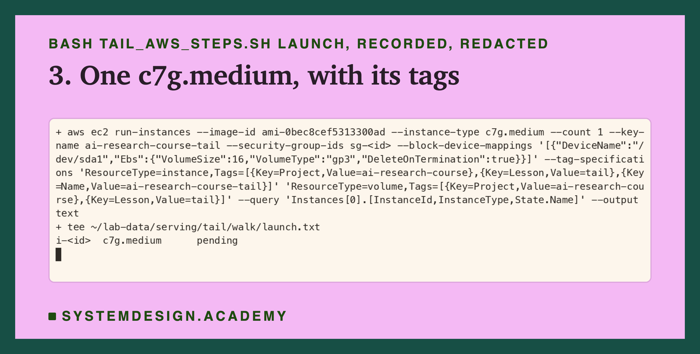
    Step 3: rent the box. First the step asks AWS for the id of today's Ubuntu 24.04 image for arm processors. Canonical, the company behind Ubuntu, publishes that id in a public AWS setting, so you never need to copy an image id from a web page. On the day I ran the lab it returned ami-0bec8cef5313300ad, the image the lab used.

    Then run-instances asks for one c7g.medium with that image and a 16 GiB disk that is deleted with the box. The disk is gp3, AWS's standard kind of SSD disk. The step also sets two tags, labels that say which project and lesson the box belongs to. The tags are how step 1 and step 13 find it again.

    A real terminal recording of step 3, with the group and instance ids replaced by placeholders. The command aws ec2 run-instances with the Ubuntu image ami-0bec8cef5313300ad, type c7g.medium, the key ai-research-course-tail, a 16 GiB gp3 disk deleted on termination, and the tags Project, Lesson and Name. It prints the new instance's id, c7g.medium and pending.

    AMI=$(aws ssm get-parameters \
      --names /aws/service/canonical/ubuntu/server/24.04/stable/current/arm64/hvm/ebs-gp3/ami-id \
      --query "Parameters[0].Value" --output text)
    ID=$(aws ec2 run-instances --image-id "$AMI" --instance-type c7g.medium --count 1 \
      --key-name "$NAME" --security-group-ids "$SG" \
      --block-device-mappings '[{"DeviceName":"/dev/sda1","Ebs":{"VolumeSize":16,"VolumeType":"gp3","DeleteOnTermination":true}}]' \
      --tag-specifications \
      "ResourceType=instance,Tags=[{Key=Project,Value=ai-research-course},{Key=Lesson,Value=tail},{Key=Name,Value=$NAME}]" \
      "ResourceType=volume,Tags=[{Key=Project,Value=ai-research-course},{Key=Lesson,Value=tail}]" \
      --query "Instances[0].InstanceId" --output text)
    echo "ID=$ID" >> "$STATE/vars"
    

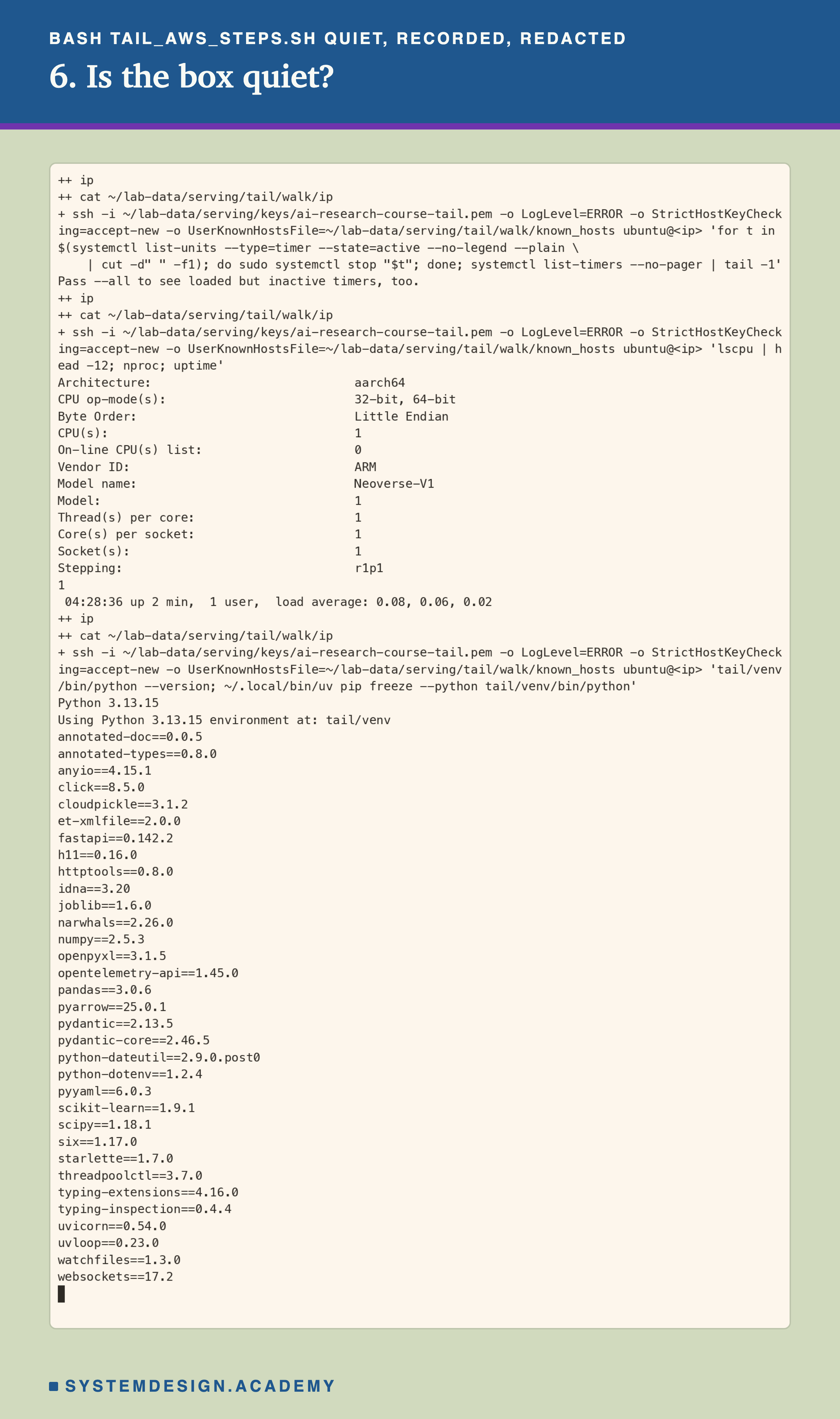
    Step 6: is the box quiet? Ubuntu runs small jobs on a timer, such as checking for updates. One of those starting in the middle of a run would land straight in the tail, so the step stops every timer first. Then it prints what the box is (lscpu), how many cores it has (nproc), how busy it has been (uptime), and every installed package with its version (pip freeze).

    A real terminal recording of step 6, with the address replaced by a placeholder. Over ssh: stop every active timer, then print the last line of systemctl list-timers, which here is only its hint, Pass --all to see loaded but inactive timers, too; lscpu prints architecture aarch64, 1 CPU, vendor ARM, model name Neoverse-V1, 1 thread per core, 1 core per socket; nproc prints 1; uptime prints up 2 min with load average 0.08, 0.06, 0.02. Then Python 3.13.15 and the full pip freeze, including fastapi 0.142.2, numpy 2.5.3, pandas 3.0.6, scikit-learn 1.9.1, starlette 1.7.0, uvicorn 0.54.0 and uvloop 0.23.0.

    ssh "${SSH[@]}" ubuntu@"$IP" 'for t in $(systemctl list-units --type=timer --state=active --no-legend --plain \
      | cut -d" " -f1); do sudo systemctl stop "$t"; done; systemctl list-timers --no-pager | tail -2'
    ssh "${SSH[@]}" ubuntu@"$IP" 'lscpu | head -12; nproc; uptime'
    ssh "${SSH[@]}" ubuntu@"$IP" 'tail/venv/bin/python --version; ~/.local/bin/uv pip freeze --python tail/venv/bin/python'
    

    Check three things: nproc prints 1, the load average is near 0, and the versions match lesson 2's lat_requirements.txt. Mine matched the measuring box line for line. In the recording, the timer list shows only its last line, a hint; the file now prints two lines, so the count of timers listed shows too.

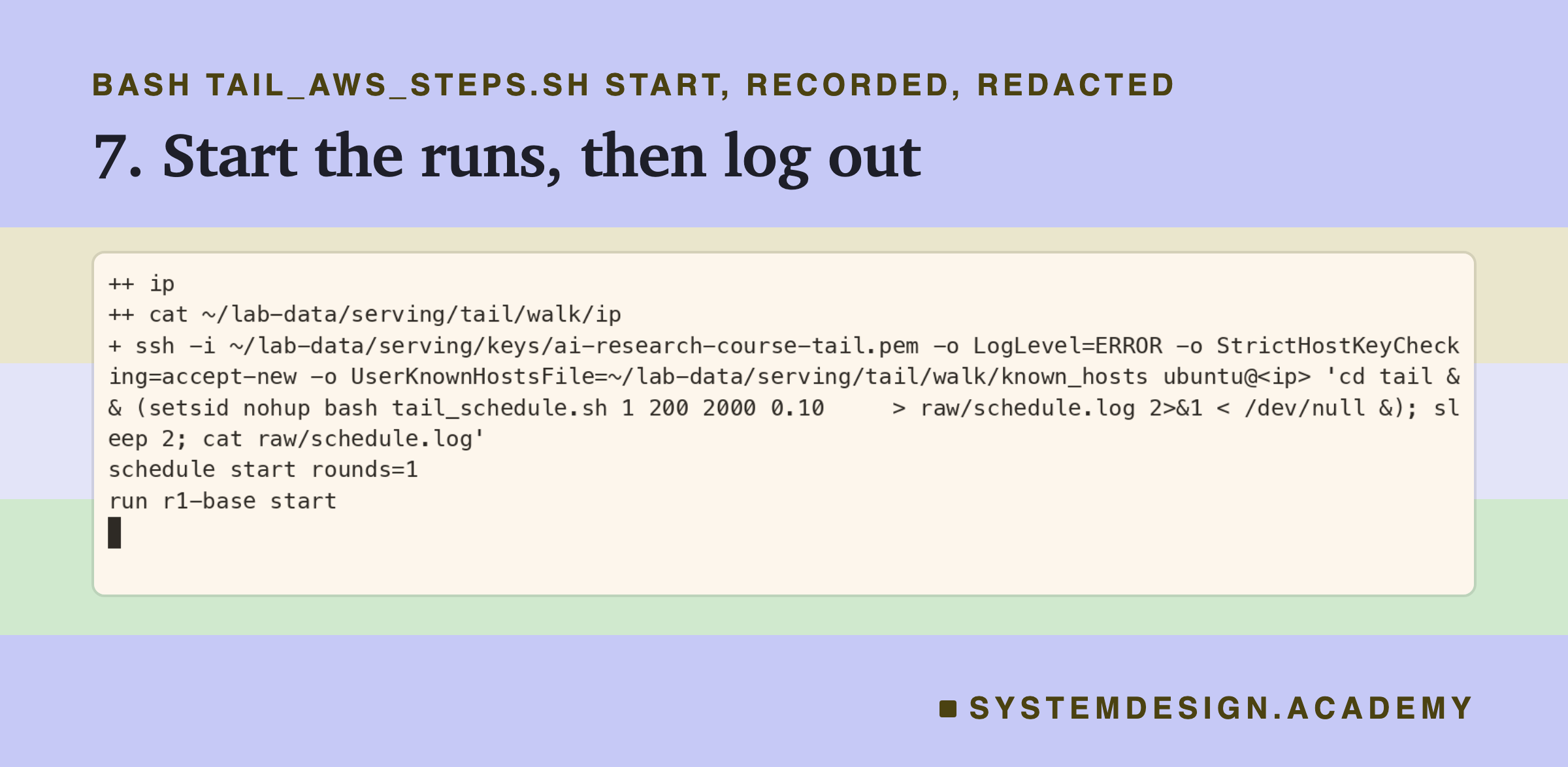
    Step 7: start the runs, then leave. The schedule starts in the background with setsid nohup, so it keeps running after SSH disconnects. Then I log out. Nobody may connect while it runs: lesson 2 showed that one SSH session was enough to move a p99.

    A real terminal recording of step 7, with the address replaced by a placeholder. Over ssh: cd tail, then setsid nohup bash tail_schedule.sh 1 200 2000 0.10 with its output sent to raw/schedule.log, in the background; two seconds later the log shows schedule start rounds=1 and run r1-base start.

    ssh "${SSH[@]}" ubuntu@"$IP" "cd tail && (setsid nohup bash tail_schedule.sh $ROUNDS $N_WARM $N_MEASURED 0.10 \
      > raw/schedule.log 2>&1 < /dev/null &); sleep 2; cat raw/schedule.log"
    

    The numbers after tail_schedule.sh are the rounds, the warm-up requests, the measured requests and the quiet limit for the load average. By default they are the lab's real values, 5, 1,000, 100,000 and 0.10. The recording box was started with ROUNDS=1 N_WARM=200 N_MEASURED=2000 in front of the command, which is why it shows 1, 200 and 2,000. While it runs, the schedule writes progress lines to the box's serial console, a log that AWS can read without logging in to the box. So I can follow it with aws ec2 get-console-output and never touch the box.

    The recorded run checked the box's own state ("terminated") instead of counting boxes with the lesson's tag; the other three checks are the same.

    cron
    AWS

    One possible reason is that something else was using the processor's shared parts: the caches, the memory, or the machine under the box. AWS says Graviton3 has "dedicated caches for every vCPU", but the memory and the host are still shared. I did not measure that, so it stays a guess.

    r"""Why is p99 so far from the median? Send 20,000 requests to a small model service and look at the slowest ones.
    
    Lesson 3 of 'Serving and Inference Basics'. It uses lesson 2's Python environment, made once inside this folder
    (Python 3.13 is what the lab used):
        python3 -m venv venv-sv
        source venv-sv/bin/activate              # Windows: venv-sv\Scripts\activate
        pip install -r lat_requirements.txt      # numpy, pandas, pyarrow, scikit-learn, fastapi, uvicorn, ...
    It also needs the shop data from the features chapter: run python ../../features/fetch_data.py once first. Then:
        python tail_demo.py                  # print the tail and what sits in it
        python tail_demo.py --save out.json  # and save the numbers
    If a package is missing, or the service does not start, it prints one line saying why and stops.
    The timings it prints come from YOUR machine, as it is right now: other programs move them. It writes only to a
    temporary folder (deleted at the end) and to out.json if you ask.
    
    Design, written 2026-10-02 after the lab's design (tail_latency.py) and before this file first ran:
      1. Train the features chapter's model (it must score test AP 0.5450), pickle it, and put every test row's six
         features into SQLite, in a temporary folder (as lesson 2's lat_demo.py does; its build step is copied here).
      2. Start the service in a SECOND Python process (this file with --serve): lesson 2's handler under uvicorn, one
         worker, with a gc.callbacks hook that records the start and stop of every garbage collection in the service.
      3. From this process, with this process's own garbage collector off, send 20,000 requests one at a time over one
         kept-alive connection, each written in one piece. NO warm-up: the first requests a fresh service sees are in.
      4. Print the round trip's p50, p90, p99, p99.9 and max; how many of the slowest 1% had a garbage collection in the
         service during them, and how many of all requests did; how many of the slowest 1% were among the first 1%; and
         for pages of 10 calls in a row, the share with at least one call over p99 next to 1 - (1 - f)^10.
    
    Author: Roni Das
    Created: 2026-10-02
    """
    import gc
    import importlib.util
    import json
    import os
    import pickle
    import socket
    import sqlite3
    import subprocess
    import sys
    import tempfile
    import time
    from pathlib import Path
    from time import perf_counter_ns
    
    NEEDED = ("numpy", "pandas", "pyarrow", "sklearn", "fastapi", "uvicorn", "pydantic")
    missing = [m for m in NEEDED if importlib.util.find_spec(m) is None]
    if missing:
        sys.exit(f"tail_demo.py needs {', '.join(missing)}: make the environment in its docstring "
                 f"(pip install -r lat_requirements.txt), then run it with that environment's python.")
    
    import numpy as np  # noqa: E402
    
    COLS = ("recency_days", "frequency", "money", "return_share", "tenure_days", "products")
    N = 20_000
    PAGE = 10
    
    
    # ───────────── the service: runs in its own process, started with --serve <folder> <port> ─────────────
    def serve(folder: Path, port: int) -> None:
        import uvicorn
        from fastapi import FastAPI, Request
        from pydantic import BaseModel
        from starlette.responses import Response
    
        class ScoreRequest(BaseModel):
            id: int
            customer_id: int
            cutoff: str
    
        model = pickle.loads((folder / "model.pkl").read_bytes())
        db = sqlite3.connect(folder / "store.sqlite", check_same_thread=False)
        sql = f"SELECT {', '.join(COLS)} FROM features WHERE customer_id = ? AND cutoff = ?"
        pauses, started = [], [0]
    
        def on_gc(phase, info):
            if phase == "start":
                started[0] = perf_counter_ns()
            else:
                pauses.append((started[0], perf_counter_ns(), info["generation"]))
    
        gc.callbacks.append(on_gc)
        app = FastAPI()
    
        @app.post("/score")
        async def score(request: Request) -> Response:
            req = ScoreRequest.model_validate_json(await request.body())
            feats = db.execute(sql, (req.customer_id, req.cutoff)).fetchone()
            p = float(model.predict_proba(np.array([feats], dtype=np.float64))[0, 1])
            out = json.dumps({"id": req.id, "customer_id": req.customer_id, "cutoff": req.cutoff, "score": p}).encode()
            return Response(content=out, media_type="application/json")
    
        @app.get("/health")
        async def health() -> Response:
            return Response(content=b"ok")
    
        @app.get("/pauses")
        async def get_pauses() -> Response:
            return Response(content=json.dumps(pauses).encode(), media_type="application/json")
    
        uvicorn.run(app, host="127.0.0.1", port=port, workers=1, access_log=False, log_level="warning")
    
    
    # ───────────── everything else runs here ─────────────
    def build(folder: Path):
        """Lesson 2's lat_demo.py build step: the model, the SQLite store, the requests in the lab's order."""
        from sklearn.metrics import average_precision_score
        here = Path(__file__).resolve().parent
        sys.path.insert(0, str(here.parents[1] / "features"))
        import task
        from what_a_feature_is import HAND_COLS, hgb, joined
    
        ev = task.load_events()
        lab_tr, _, lab_te = task.splits(ev)
        tr = joined(ev, lab_tr, task.TRAIN_CUTOFFS)
        te = joined(ev, lab_te, task.TEST_CUTOFFS)
        model = hgb(0).fit(tr[HAND_COLS].to_numpy(float), tr["label"].to_numpy())
        p = model.predict_proba(te[HAND_COLS].to_numpy(float))[:, 1]
        y, cut = te["label"].to_numpy(), te["cutoff"].to_numpy()
        ap = float(np.mean([average_precision_score(y[cut == c], p[cut == c]) for c in np.unique(cut)]))
        assert round(ap, 4) == 0.5450, ap
        (folder / "model.pkl").write_bytes(pickle.dumps(model, protocol=5))
        day = te["cutoff"].dt.strftime("%Y-%m-%d").to_numpy()
        con = sqlite3.connect(folder / "store.sqlite")
        con.execute("CREATE TABLE features (customer_id INTEGER, cutoff TEXT, "
                    + ", ".join(f"{c} REAL" for c in COLS) + ", PRIMARY KEY (customer_id, cutoff))")
        con.executemany("INSERT INTO features VALUES (?, ?, ?, ?, ?, ?, ?, ?)",
                        [(int(c), d, *map(float, r)) for c, d, r in zip(te["customer_id"], day, te[HAND_COLS].to_numpy())])
        con.commit()
        con.close()
        order = np.random.default_rng(0).permutation(len(te))   # the lab's request order
        pairs = [(int(te["customer_id"].iloc[i]), str(day[i])) for i in order[np.arange(N) % len(te)]]
        return ap, pairs
    
    
    def wait_until_up(svc, port: int, log: Path, limit_s: float = 60.0) -> str:
        """Wait for GET /health. Return "" when it answers, else one line saying why it did not."""
        start = time.monotonic()
        while time.monotonic() - start < limit_s:
            if svc.poll() is not None:
                lines = [ln for ln in log.read_text(errors="replace").splitlines() if ln.strip()]
                return f"it exited with code {svc.returncode}: {lines[-1] if lines else 'no message'}"
            try:
                with socket.create_connection(("127.0.0.1", port), timeout=2) as c:
                    c.sendall(b"GET /health HTTP/1.1\r\nHost: x\r\n\r\n")
                    if c.recv(4096).endswith(b"ok"):
                        return ""
            except OSError:
                pass
            time.sleep(0.2)
        return f"no answer on port {port} after {limit_s:.0f} s"
    
    
    def exchange(sock: socket.socket, msg: bytes) -> bytes:
        """Send one whole HTTP message, read one whole answer (its Content-Length says how long)."""
        sock.sendall(msg)
        buf = b""
        while True:
            chunk = sock.recv(65536)
            if not chunk:
                raise OSError("the service closed the connection")
            buf += chunk
            h = buf.find(b"\r\n\r\n")
            if h >= 0:
                head = buf[:h].lower()
                k = head.find(b"content-length:")
                end = head.find(b"\r\n", k)
                need = h + 4 + int(head[k + 15:end if end > 0 else None])
                if len(buf) >= need:
                    return buf[h + 4:need]
    
    
    def main() -> None:
        try:
            load = f"{os.getloadavg()[0]:.2f}"
        except (AttributeError, OSError):
            load = "not available on this system"
        print(f"Every time below was measured on THIS machine ({os.cpu_count()} CPUs, 1-minute load {load}).")
        with tempfile.TemporaryDirectory() as tmp:
            folder = Path(tmp)
            ap, pairs = build(folder)
            print(f"model trained: test AP {ap:.4f}; {len(pairs):,} requests ready, no warm-up")
            with socket.socket() as s:
                s.bind(("127.0.0.1", 0))
                port = s.getsockname()[1]
            log = open(folder / "service.log", "w")
            svc = subprocess.Popen([sys.executable, __file__, "--serve", str(folder), str(port)],
                                   stdout=log, stderr=subprocess.STDOUT)
            try:
                why = wait_until_up(svc, port, folder / "service.log")
                if why:
                    sys.exit(f"the service did not start: {why}")
                head = "POST /score HTTP/1.1\r\nHost: x\r\nContent-Type: application/json\r\nContent-Length: {}\r\n\r\n"
                msgs = []
                for i, (c, d) in enumerate(pairs):
                    b = json.dumps({"id": 1_000_000 + i, "customer_id": c, "cutoff": d}).encode()
                    msgs.append(head.format(len(b)).encode() + b)
                sock = socket.create_connection(("127.0.0.1", port), timeout=30)
                sock.setsockopt(socket.IPPROTO_TCP, socket.TCP_NODELAY, 1)
                t = np.zeros((N, 2), dtype=np.int64)
                gc.collect()
                gc.disable()
                for i, m in enumerate(msgs):
                    a = perf_counter_ns()
                    exchange(sock, m)
                    t[i] = (a, perf_counter_ns())
                gc.enable()
                pauses = np.array(json.loads(exchange(sock, b"GET /pauses HTTP/1.1\r\nHost: x\r\n\r\n")),
                                  dtype=np.int64).reshape(-1, 3)
                sock.close()
            except OSError as e:
                sys.exit(f"the service stopped answering ({type(e).__name__}: {e}); see the docstring")
            finally:
                svc.terminate()
                svc.wait()
                log.close()
    
        rt = (t[:, 1] - t[:, 0]) / 1000
        q = {name: float(np.percentile(rt, p)) for name, p in (("p50", 50), ("p90", 90), ("p99", 99), ("p99.9", 99.9))}
        q["max"] = float(rt.max())
        print(f"\nround trip of {N:,} requests, one at a time, in microseconds (us):")
        for name, v in q.items():
            print(f"  {name:6s} {v:10.1f}   {v / q['p50']:5.2f} x the median")
    
        # did a collection in the service overlap the request?
        hit = np.zeros(N, dtype=bool)
        for s0, s1, _ in pauses:
            hit |= (t[:, 0] <= s1) & (t[:, 1] >= s0)
        slow = rt >= q["p99"]
        first = np.arange(N) < N // 100
        gens = np.bincount(pauses[:, 2], minlength=3) if len(pauses) else np.zeros(3, int)
        print(f"\ngarbage collections in the service: {len(pauses)} (generation 0: {gens[0]}, 1: {gens[1]}, 2: {gens[2]})")
        print(f"  a collection ran during {hit[slow].mean():6.1%} of the slowest 1%, and during {hit.mean():6.1%} of all")
        print(f"  the first 1% of requests made up {first[slow].mean():6.1%} of the slowest 1%")
    
        f = float(slow.mean())
        pages = slow[: N // PAGE * PAGE].reshape(-1, PAGE).any(axis=1)
        print(f"\npages of {PAGE} calls in a row: share with at least one call at or over p99")
        print(f"  measured {pages.mean():.4f};  1 - (1 - {f:.4f})^{PAGE} = {1 - (1 - f) ** PAGE:.4f}")
        if "--save" in sys.argv:
            out = {"load": load, "cpus": os.cpu_count(), "test_ap": ap, "n": N, "quantiles_us": q,
                   "collections": int(len(pauses)), "by_generation": [int(x) for x in gens],
                   "gc_share_slowest": float(hit[slow].mean()), "gc_share_all": float(hit.mean()),
                   "first_share_slowest": float(first[slow].mean()), "f": f, "pages_measured": float(pages.mean()),
                   "pages_predicted": 1 - (1 - f) ** PAGE}
            Path(sys.argv[sys.argv.index("--save") + 1]).write_text(json.dumps(out, indent=1))
    
    
    if __name__ == "__main__":
        if len(sys.argv) > 1 and sys.argv[1] == "--serve":
            serve(Path(sys.argv[2]), int(sys.argv[3]))
        else:
            main()
    

    Here is the demo running on the recording box, quiet, with a real terminal recorder. This exact run is stored in results/tail-demo-run.txt.

    A terminal recording of python tail_demo.py run on the recording box. It prints: every time below was measured on this machine, 1 CPU, 1-minute load 0.03; model trained, test AP 0.5450, 20,000 requests ready, no warm-up. Round trip of 20,000 requests, one at a time, in microseconds: p50 901.8, 1.00 x the median; p90 914.6, 1.01 x; p99 930.4, 1.03 x; p99.9 981.9, 1.09 x; max 6402.8, 7.10 x. Garbage collections in the service: 2, generation 0: 1, 1: 1, 2: 0; a collection ran during 0.0% of the slowest 1% and 0.0% of all; the first 1% of requests made up 23.0% of the slowest 1%. Pages of 10 calls in a row: measured 0.0785; 1 - (1 - 0.0100)^10 = 0.0956. Caption: recorded on the box; this exact run is in results/tail-demo-run.txt.

    On that box, the demo printed: the service made 2 collections in its whole life, during none of the requests. The max was 7.10 times the median, and pages of 10 met the tail less often than the formula, 0.0785 against 0.0956. In this one demo run, the first 1% of requests made up 23.0% of the slowest 1%. One demo run is one data point, so I do not read more into it. The report checks that the stored text and the demo's saved numbers agree.

    And here is the same demo in VS Code on my laptop, run with python tail_demo.py in the examples folder with venv-sv active.

    A real screenshot of VS Code's terminal on my laptop, in the venv-sv environment, after python tail_demo.py. Its first line says every time was measured on this machine, 10 CPUs, 1-minute load 3.09. The model trained to test AP 0.5450. The round trip of 20,000 requests, in microseconds: p50 2059.3, p90 2686.0, p99 3339.0 (1.62 x the median), p99.9 3951.6, max 10902.6. Garbage collections in the service: 2, one in generation 0 and one in generation 1; a collection ran during 0.0% of the slowest 1% and 0.0% of all requests; the first 1% of requests made up 0.5% of the slowest 1%. Pages of 10 calls in a row: measured 0.0805, against 1 - (1 - 0.0100)^10 = 0.0956.

    My laptop was busy with other work when I took this. The demo's first line says 10 CPUs and a 1-minute load of 3.09. Other programs shared the processor during the run, so these are not quiet-machine times. I do not set them beside any other number in this lesson.

    Read the screen only for what the demo prints, as you will read your own. The service made 2 collections, and none ran during a request. Pages of 10 calls in a row met the tail 0.0805 of the time. The formula says 0.0956.

    Your times will be different. Look at the same three things. How far is the max from the median? Did any collection run during a request? Did pages meet the tail more or less often than the formula?

    gc.callbacks
    gc.freeze()

    tail_files/tail_client.py is the client, a second process. It builds every request first, turns its own garbage collector off, and then sends one request at a time over one open connection, each request in one piece. After the run it asks the service for its stored readings and saves everything in one file.

    tail_files/tail_run_once.sh waits until the box is quiet, starts a fresh service with the arm's settings, runs the client, and stops the service. It also records the load, the CPU counters and the system log during the run. tail_files/tail_schedule.sh runs all the arms, five rounds, in a rotated order.

    tail_report.py does not import any of the above. It rebuilds every clock reading from the raw files with its own code and recomputes every number. It also checks the guesses, the demo's stored run and the fact-check, and writes the playground.

  • Change one thing, in paired runs, with a rule written first. When the runs disagree, say "cannot be told apart from run-to-run noise".

  • def