Let me start in a coffee shop.

You walk in, order a coffee, and pay. Some minutes later, you have the cup in your hand. The coffee machine itself only ran for a short part of that time. So where did the rest of the wait go?

Many small things happened. The person at the till typed your order. A slip went to the person making drinks. Someone took milk from the fridge. The machine ran. Your name was called, and you walked to the counter. Each step is short. Together they make the wait.

If the shop wants faster coffee, buying a faster machine may not help much. Maybe the till is slow, or the slips wait in a pile. The owner first needs to know which step takes the time. Then they can fix the right one.

A prediction service is like that shop. A request comes in, many small steps happen, and an answer goes out. In this lesson I time every one of those steps, on a real service with a real model, and I find out where the time goes.

This is lesson 2 of the chapter on serving. Lesson 1, batch or online, asked whether to score every customer in a nightly batch or each request as it comes. This lesson takes the second choice, scoring each request as it comes, and looks inside one request.

The model is the one from the features chapter. If it is new to you, please read what a feature is first. It uses six features of each customer of a real online shop, built from their past invoices. It answers one question: at the start of a month, will this customer buy something in the next 30 days? It is a gradient boosted tree model from scikit-learn, and it scored a test AP of 0.5450. AP, average precision, is a score from 0 to 1 for how well the model ranks the buyers above the others.

The survey lesson model serving and inference APIs has a slide called "The Request Path". It walks a request through a gateway, a cache, a feature store and a model, and it gives example times for each hop. I will not repeat that slide here. Instead, I build a small version of that path and measure it.

Please read this slide slowly if any word is new. Every slide after it uses these words.

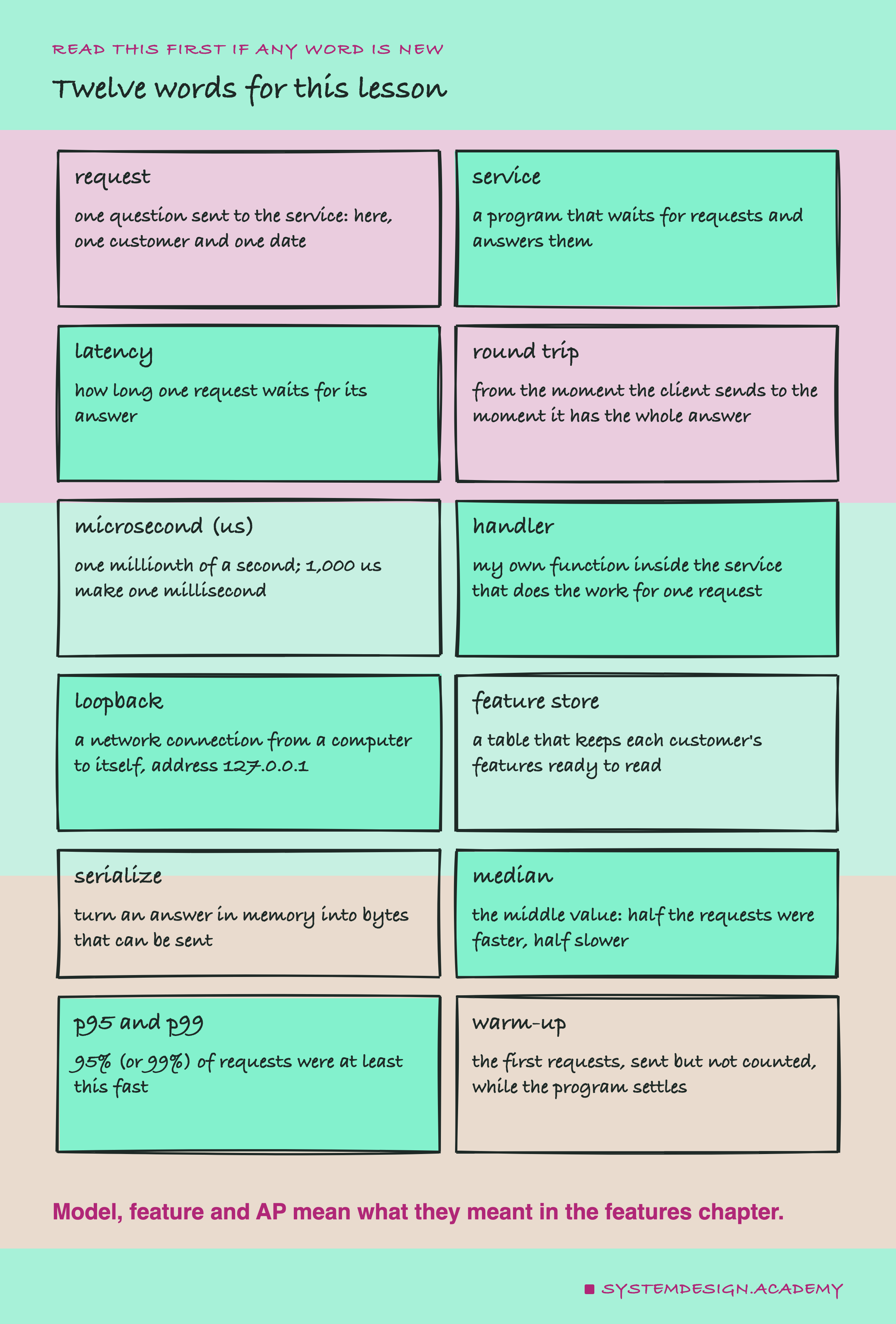
A service is a program that waits for questions and answers them. Each question is a request. The program that sends requests is the client. Here the client is a small Python program, and the service is a web server that holds the model.

Latency is how long one request waits for its answer. The round trip is latency as the client sees it: from the moment it sends the request until it has read the whole answer. Think of the coffee: from paying until the cup is in your hand.

The times in this lesson are very short, so I use the microsecond. One microsecond is one millionth of a second. A thousand microseconds make one millisecond. The figures write microseconds as "us".

The handler is the one function I wrote inside the service. Everything else in the service, such as reading the network and finding my function, is code from libraries. The loopback is a network connection from a computer to itself. The client and the service ran on the same machine, so their requests never left it.

When I send 20,000 requests, I get 20,000 times. The median is the middle one: half the requests were faster and half slower. The p95 is the time that 95% of requests were at or under, and the the time that 99% were at or under. The p99 tells you about the slow few, which the median hides.

Before the numbers, here is the path one request took in my service. Each arrow is a step, and the times in brackets show where my handler read the clock.

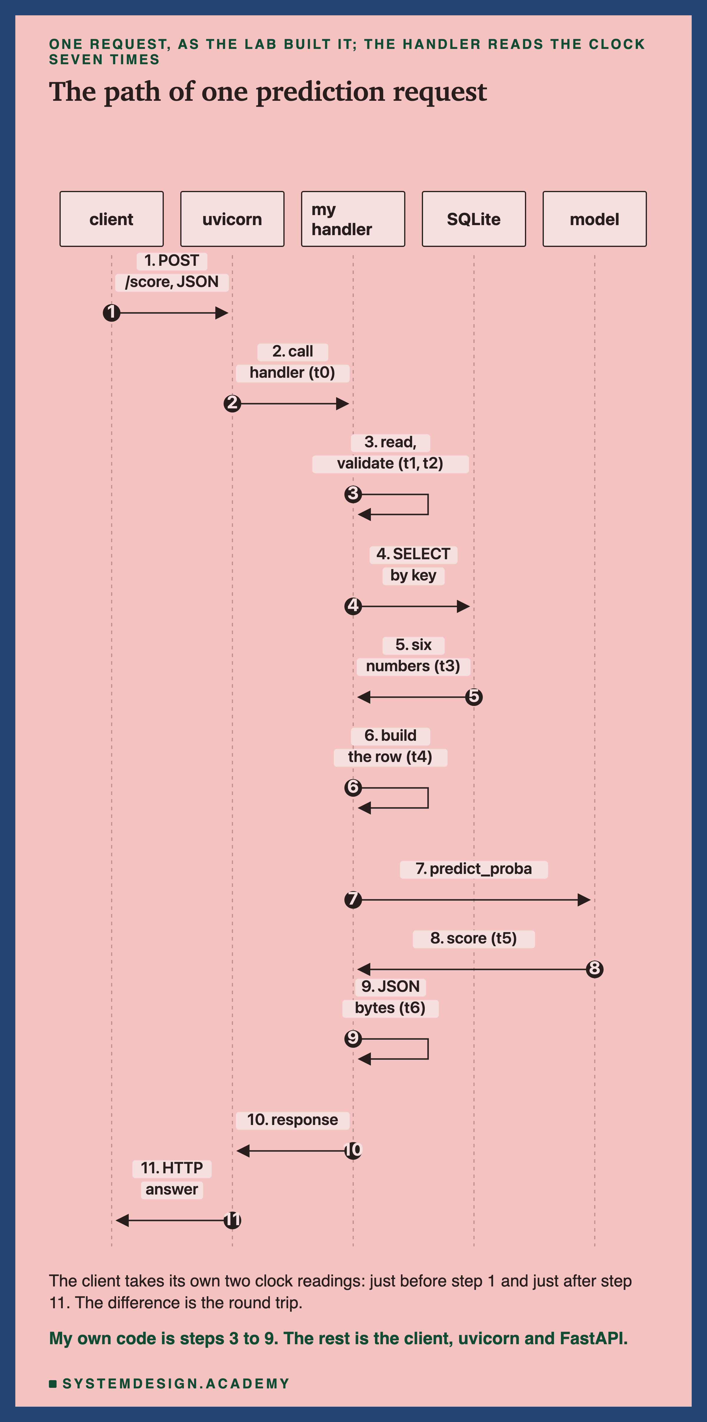
The client sends a small piece of JSON, such as a customer number and a date, to the address /score. JSON is a common text format for data. The request goes to uvicorn, a web server for Python. Uvicorn reads the bytes and hands them to FastAPI, a library that finds the right function for each address. That function is my handler.

My handler does five things. It parses the request: it reads the body and checks it has a customer number and a date. It looks up the six features of that customer at that date in SQLite, a small database kept in one file. It builds a row: a list of six numbers in the order the model expects. It calls predict, the model's predict_proba, which returns a score from 0 to 1. And it serializes the answer: it turns the score into JSON bytes. Then the answer goes back the way the request came.

At each step, my handler reads a very precise clock, Python's time.perf_counter_ns. It reads it seven times, so I can subtract one reading from the next and get the time of each step.

I wrote the lab's design into the docstring of scripts/labs/serving/latency_anatomy.py before any timed run. At that point I had started the box and nothing more. I had not run the service anywhere, and I had not timed this model's predict in this chapter.

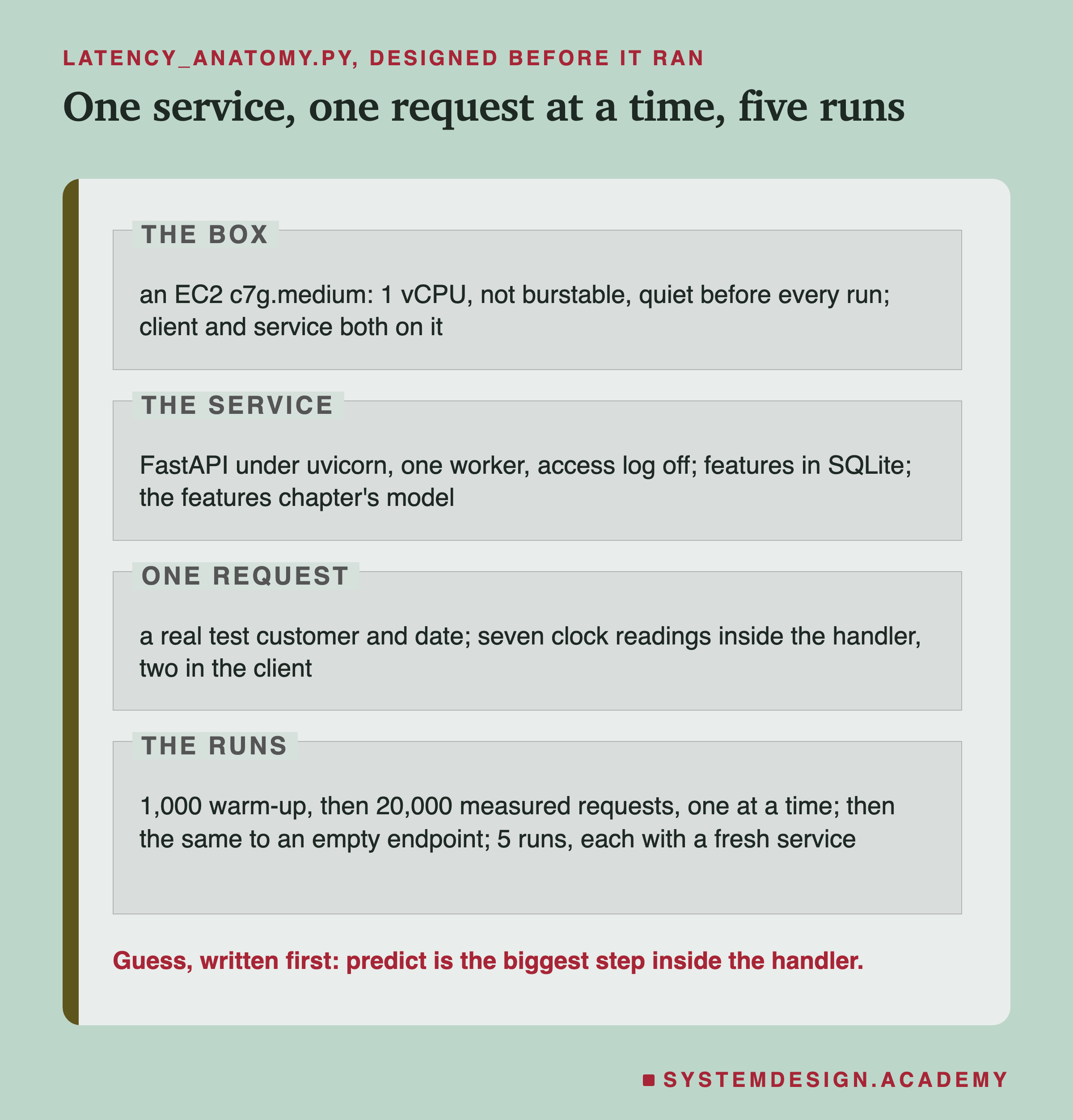
The requests are real. Each one is a real customer and a real month from the test months of the features chapter: 26,851 pairs in all. I shuffled them once, in a fixed way, and every run sent them in the same order.

One request at a time. The client sends a request, waits for the whole answer, and only then sends the next one. So no request ever waits behind another. Waiting in a line, a queue, is a real cause of slow answers, but it is a different question, and lesson 7 measures it.

A warm-up first. The first requests to a fresh program are slower, for reasons lesson 6 looks at. So each run sent 1,000 warm-up requests, which I stored but did not count, and then 20,000 measured ones.

Five runs. One run is one data point. I ran the whole thing five times, each time with a fresh service, and I report how much the runs differ.

My guesses, written first. I wrote seven guesses before the run. The main one was that predict would be the biggest step inside my handler, bigger than all the others together. I check them all near the end.

My laptop is almost always busy with other work. If I timed requests on it, I would measure my other programs as much as my service. So no timing in this lesson comes from my laptop. Every timing comes from a small machine I rented from Amazon Web Services for this lab, called an EC2 instance, or here just "the box".

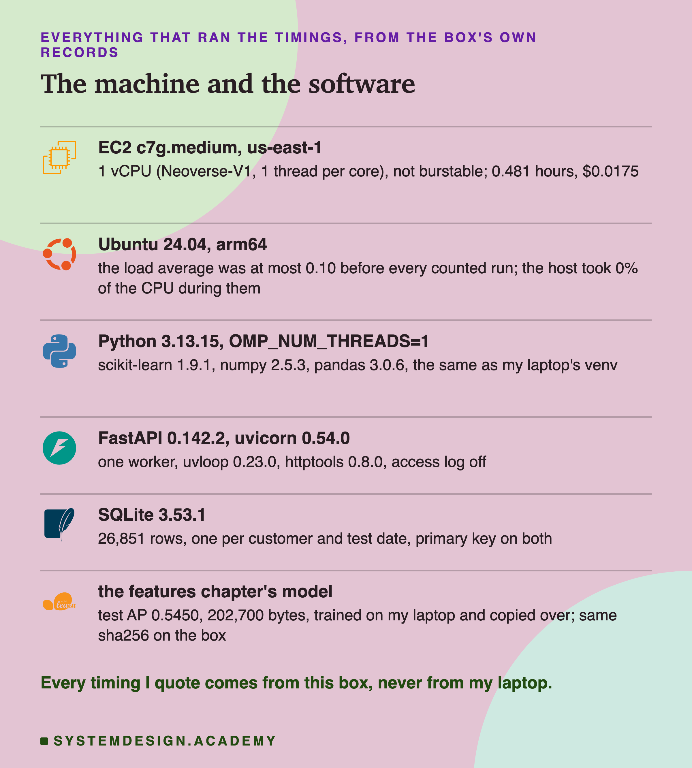
The box. The chapter plan asked for a machine with 2 virtual CPUs. My Amazon account only allows 1 virtual CPU of this kind at a time. So I used a c7g.medium. It has 1 CPU core of its own, not shared with a second thread. It is also not burstable, which means its speed does not drop after a while. One thing follows from this, and I wrote it down before running: the client and the service share that one core. So every round trip also includes the operating system switching from one program to the other and back.

The same software as my laptop. I installed the same Python, 3.13.15, and the same versions of scikit-learn, numpy and pandas. I set OMP_NUM_THREADS=1, which tells the model to use one thread, because the box has one core. I copied the model file over and checked that its sha256, a fingerprint of the file's bytes, was the same on the box.

Quiet. Before each run, the lab waited until the box's load average, a number for how busy the computer has been in the last minute, was at most 0.10. During the runs, the machine under the box took 0% of the CPU time. The box was on for 0.481 hours and cost $0.0175 for compute. Then I deleted it, with its key and its network rule.

This is a real recording of the report script, lat_report.py. It ran on my laptop, but it does no timing at all. It reads the raw timings the box measured and does the arithmetic again.

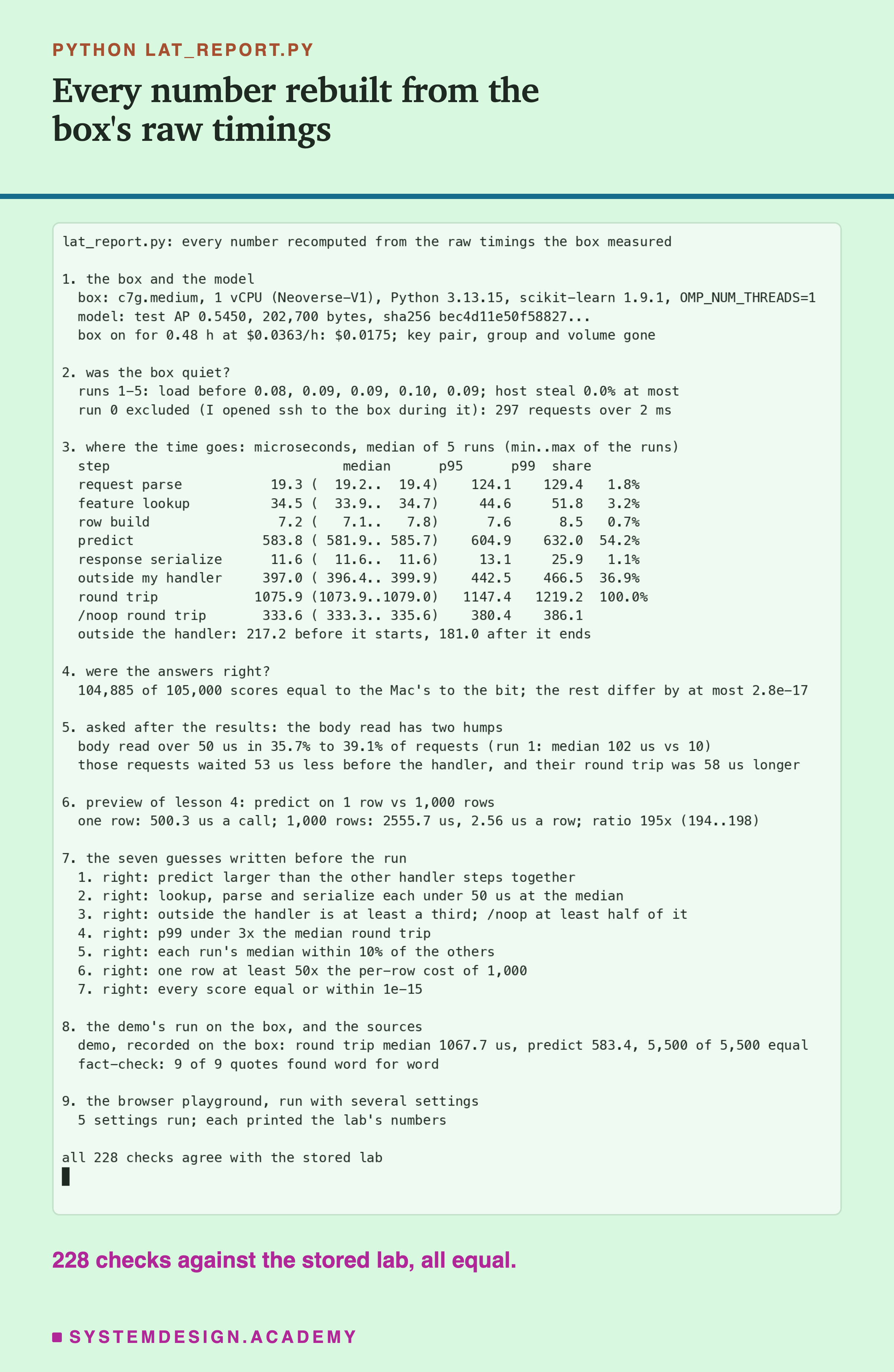
The report does not import the lab's code. It rebuilds every clock reading from the stored raw file with its own code, and it computes its own percentiles. Then it compares every number with the lab's results file, and all 228 checks agreed. It also checks the guesses, the demo's stored run and the playground further down.

Section 2 names one run I left out, run 0. I explain why on its own slide: I broke my own quiet rule during it.

Here is the main result. The bar is one request, from the moment the client sent it to the moment the client had the answer. Each piece is one step, as long as its median time.

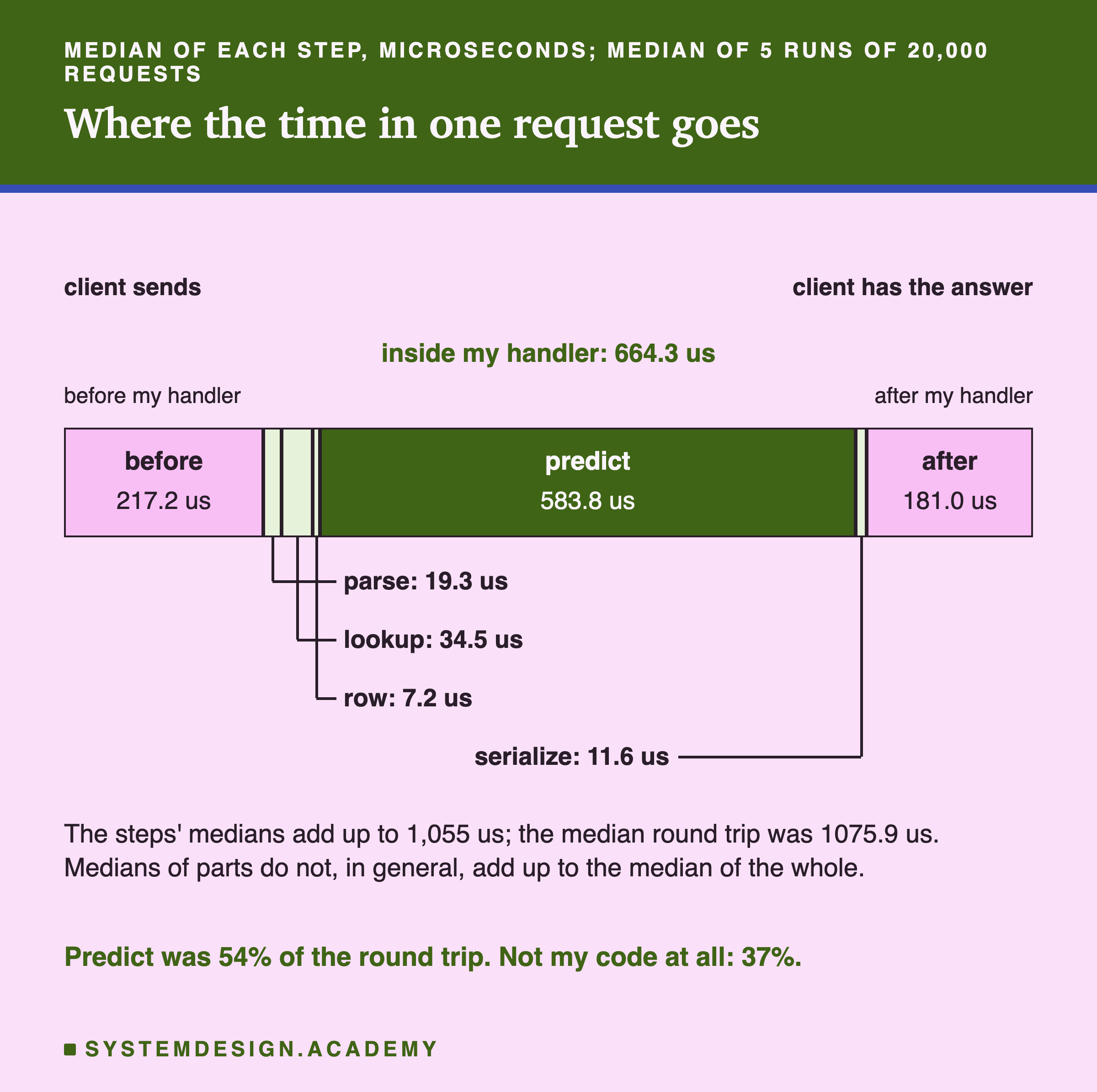
At the median, one request took 1,075.9 microseconds, about one millisecond. Here is where that time went.

Predict took 583.8 microseconds, 54% of the round trip. It was the biggest single step, by far.

Work outside my handler took 397.0 microseconds, 37%. This is the time before my function started and after it finished. It covers the client sending, the loopback, uvicorn reading the HTTP and FastAPI finding my function, and the same things on the way back.

Everything else in my handler was small. Parsing the request took 19.3 microseconds, looking up the six features in SQLite took 34.5, building the row took 7.2, and writing the JSON answer took 11.6. Together that is less than 8% of the round trip.

The seven pieces' medians, before my handler, the five steps inside it and after it, add up to 1,055 microseconds, not 1,075.9. This is not an error. The median of each part comes from a different request, so the parts' medians do not, in general, add up to the median of the whole.

The median says what a normal request did. The p99 says what the slowest 1 in 100 did. This chart shows both for every step.

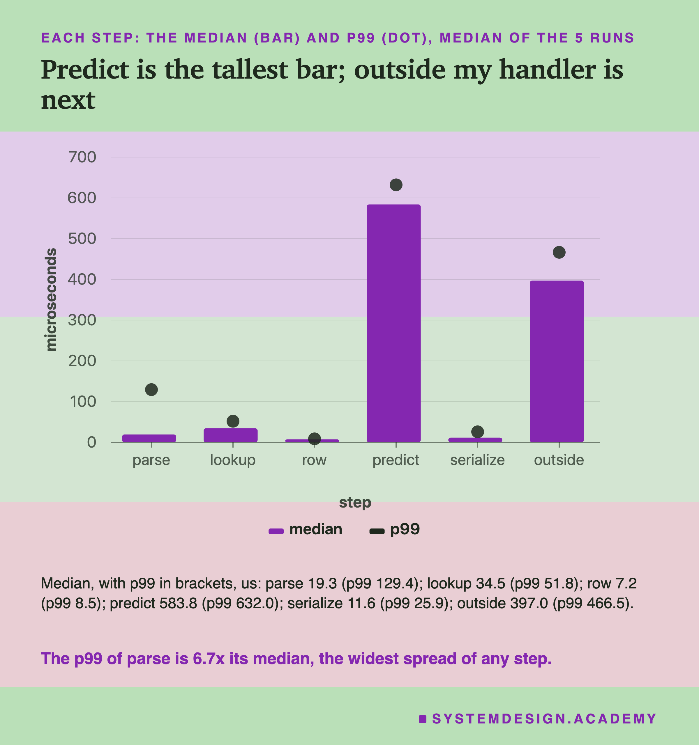
For most steps, the p99 sits close to the median. Predict's p99 was 632.0 microseconds against a median of 583.8. The work outside my handler had a p99 of 466.5 against 397.0. On a quiet box, with one request at a time, most requests took about the same time.

Parse was the exception, in this setup. Its median was 19.3 microseconds, but its p95 was 124.1 and its p99 129.4. That is more than six times the median. A step that is tiny for most requests and much bigger for others is worth a closer look. I came back to it after the main results, on the slide about two humps, which gives a likely reason tied to this client and the shared core.

For the whole round trip, the p95 was 1,147.4 microseconds and the p99 1,219.2. So the slowest 1 in 100 requests took about 13% longer than the median one. Lesson 3 looks at the slowest requests in much more detail.

Now look only inside my handler, from the first clock reading to the last.

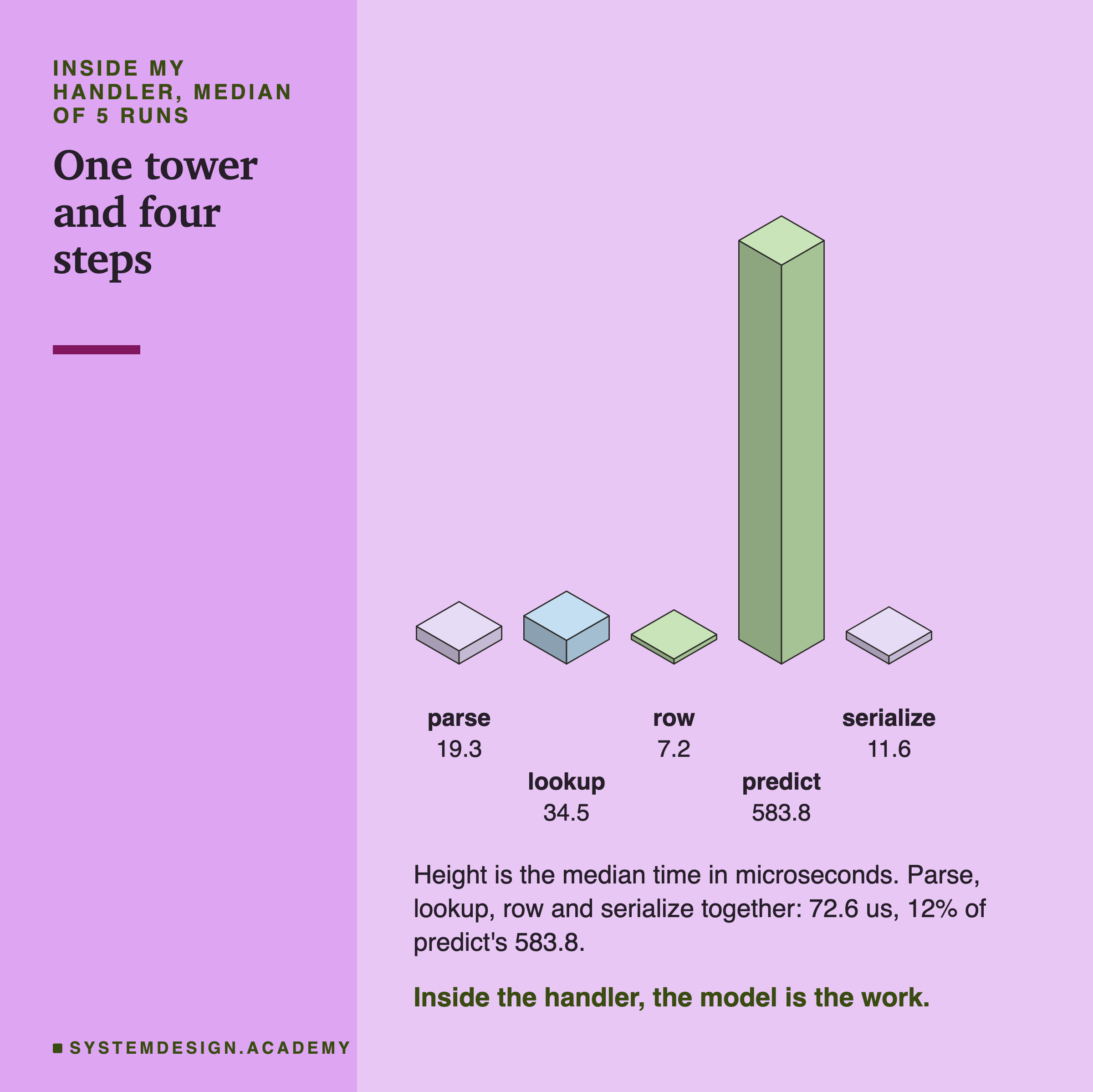
My handler took 664.3 microseconds at the median. Predict was 583.8 of them. The other four steps together took 72.6 microseconds, about 12% of predict's time.

I expected the database lookup to cost more. SQLite keeps the data in a file, and a lookup sounds like a trip to disk. But the table has 26,851 rows and a primary key on the customer and the date. A primary key builds an index, a sorted list that finds one row quickly, like the index at the back of a book.

After the warm-up, the operating system very likely keeps the whole small file in memory; I stated that in the design and did not test it. So one lookup cost 34.5 microseconds. A feature store on another machine, reached over a real network, would likely cost more. This lab does not measure that.

Why is predict so slow next to the rest? The model has 54 small trees, and one row only has to walk down each tree once. That sounds like very little work. A slide further on, the preview of lesson 4, shows that most of predict's time is not the tree walking at all.

The 397.0 microseconds outside my handler is a big share. Where in the request does it happen?

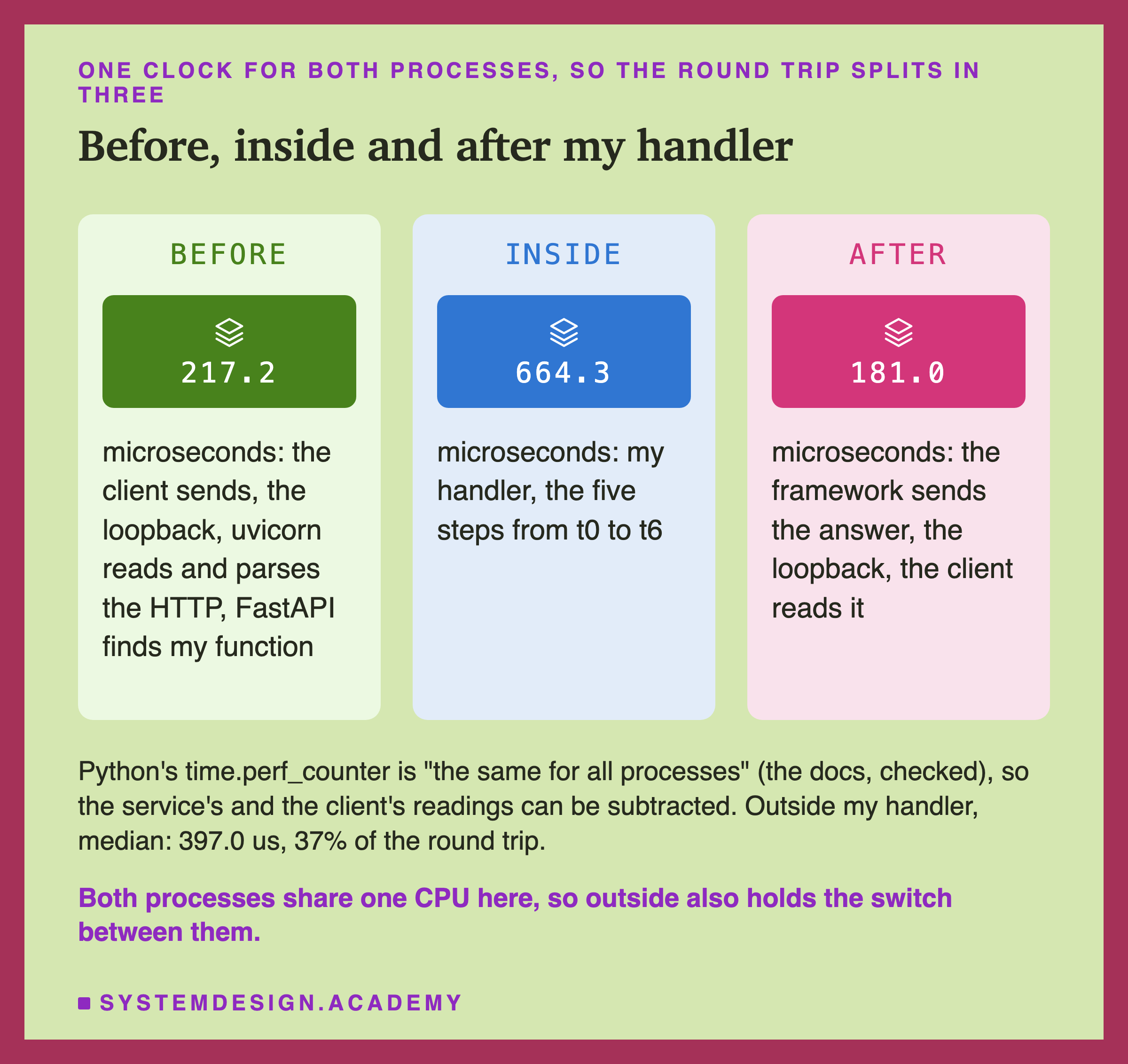
The client and the service are two separate programs. Can I subtract a clock reading in one from a clock reading in the other? Only if they read the same clock. Python's documentation says of this clock: "The clock is the same for all processes." I checked it on the box too: both programs used the operating system's monotonic clock, a clock that only ever moves forward.

So I could split the outside part in two. Before my handler started: 217.2 microseconds. In this time the client wrote the request, the operating system passed it through the loopback, uvicorn read and parsed the HTTP, and FastAPI found my function. After my handler finished: 181.0 microseconds. In this time FastAPI and uvicorn sent the answer, and the client read it.

One part of this belongs to the box I chose. With one core, the operating system must stop the client to run the service, and then stop the service to run the client.

Whatever work the client still does after it sends a request cannot run at the same time as the service, so it lands in "before my handler". On a machine where each program has its own core, some of that work would overlap. I did not measure the switch or the client's leftover work on their own, so I cannot say how much of the 397.0 microseconds they are.

To size the outside part, I added a second address to the service, /noop. Its handler does no work at all: it returns two fixed bytes. The client timed it in the same way, 20,000 times per run. This is a control: the same measurement with the thing I study taken out.

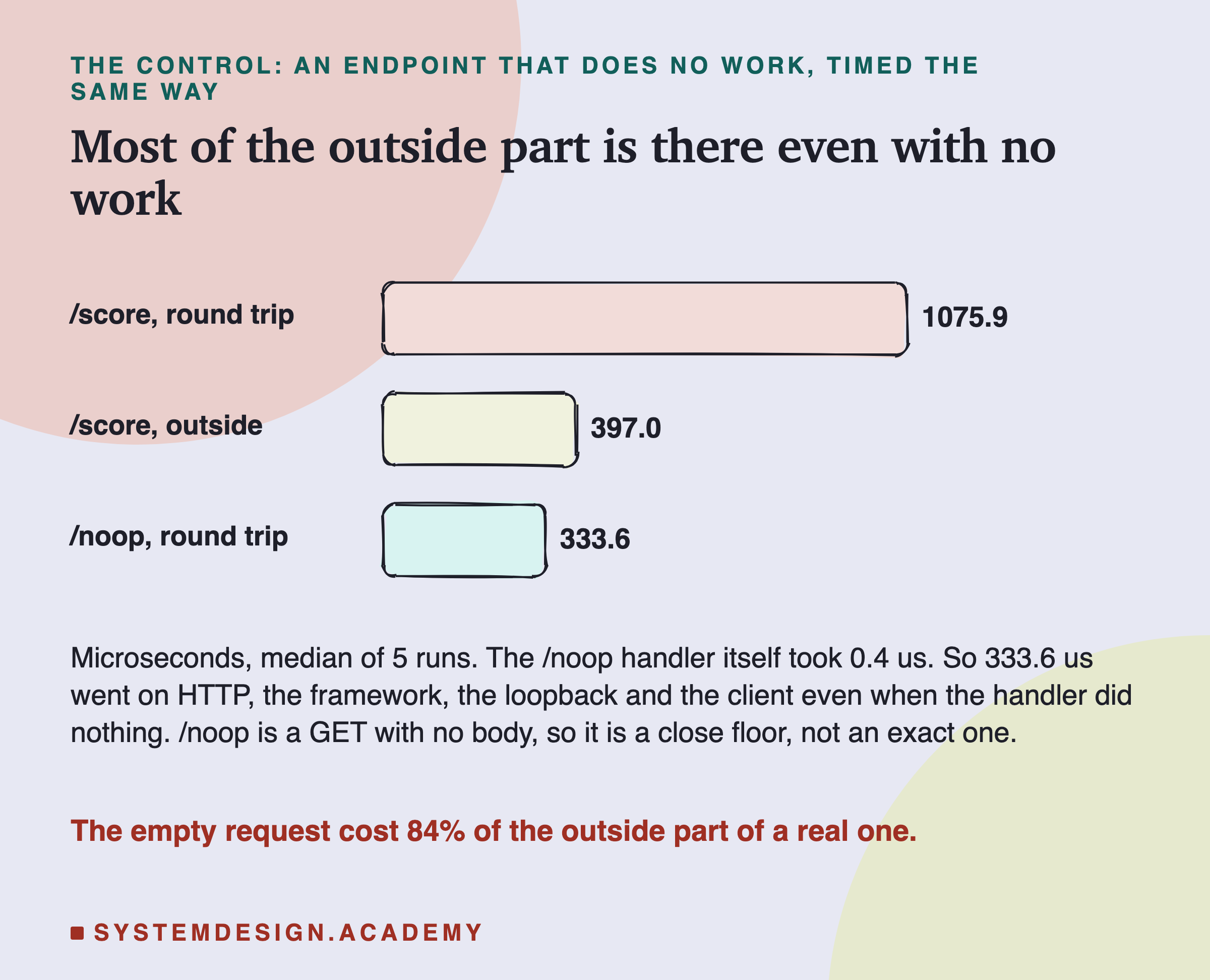
The empty request took 333.6 microseconds at the median. Its handler took 0.4 of them. So almost all of that time is the cost of being a web service at all: HTTP, the framework, the loopback, the client, and the switch between programs.

That is 84% of the 397.0 microseconds outside my handler for a real request. The real request sends a small JSON body and gets a slightly longer answer, so it is not a perfect copy. But it tells me that most of the outside part is a floor. Making my handler faster would not touch it.

This is a useful habit in real work. Before you try to speed up a service, time an endpoint that does nothing. If the empty one is already slow, the problem is not in your handler.

This slide is a finding I did not plan. The lab labels it as asked after the results.

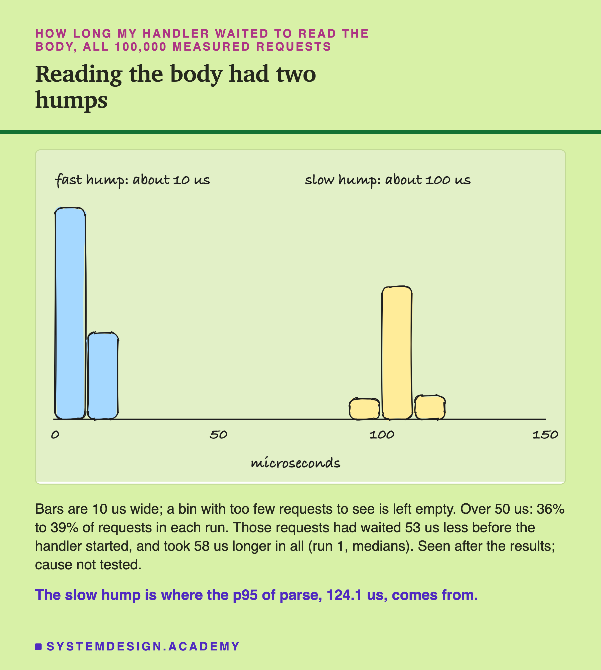
The parse step has two parts: reading the body bytes, and checking them. The checking took about 9 microseconds every time. The reading did not. In most requests it took about 10 microseconds. But in 36% to 39% of requests, in every run, it took about 100.

Then I looked at the same requests from the outside. The slow ones had waited 53 microseconds less before my handler started. So in those requests, my handler started earlier, and then waited inside for the body to be handed over. Much of the time moved from "before my handler" into "reading the body". But not all of it: the slow requests' round trip was 58 microseconds longer at the median.

I did not test why, but there is a likely reason, and it is a hypothesis only. Python's http.client, which my client used, sends a request's headers and its body in two separate send calls. It also turns off the network's habit of holding small pieces back to join them (TCP_NODELAY). I read this in Python 3.13's source.

So the headers can arrive first, the service can wake up and start my handler, and my handler then waits for the body. On one shared core, the client must run again to send the body. That fits the numbers: the slow group started about 53 microseconds earlier, read about 92 microseconds longer, and finished about 58 microseconds later. I report the two humps because they explain the parse step's wide p95 in this setup. A different client, or separate cores, could remove them.

Did the five runs agree? And what happened to run 0?

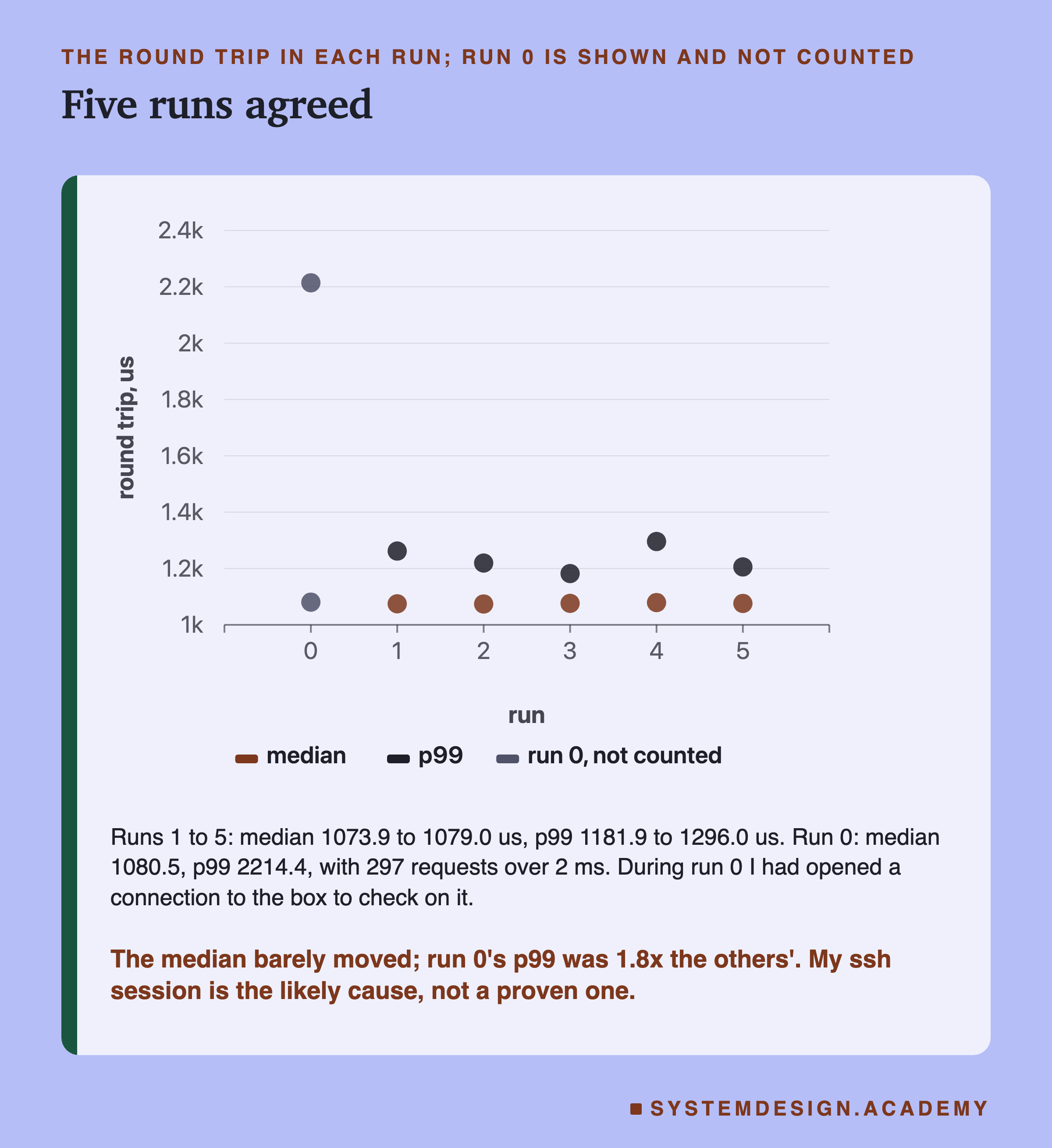
The five counted runs agreed closely. Their median round trips were between 1,073.9 and 1,079.0 microseconds. Their p99s were between 1,181.9 and 1,296.0.

Run 0 is the run I left out. While it was running, I opened a connection to the box, with ssh, a tool for working on another computer, to see if the lab was still going. That broke the quiet rule I had written into the design. Run 0 then had 297 requests over 2 milliseconds, 288 of them among its last 2,000 requests. The counted runs had 1 to 9 each. Its median was normal, 1,080.5, but its p99 was 2,214.4.

So I ran one more run, run 5, in the same way, with nobody connected. The headline uses runs 1 to 5. I kept run 0's raw timings and I show it here, so you can see what one extra small program did to the tail. My ssh session is the likely cause of run 0's slow requests, but I did not prove it.

A timing is only as good as the machine it was taken on. Here is what the box reported for each counted run.

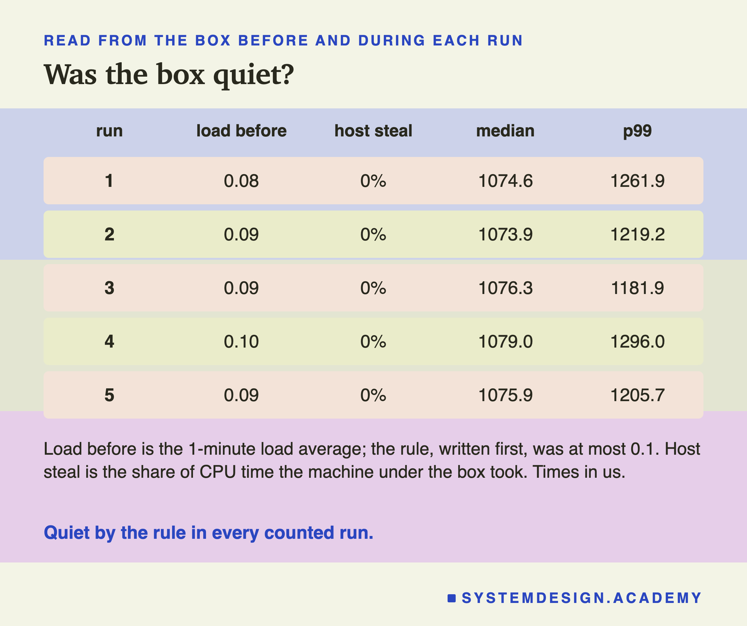
Load before is the 1-minute load average just before the run started. The rule I wrote first was at most 0.10, and every counted run met it. The lab waited between 45 and 105 seconds each time for the box to settle.

Host steal is the share of time that the real computer under my rented box gave to someone else. A rented machine runs on a bigger shared computer, and when that computer is busy, it can take time away. Here it took none.

Were the answers right? A fast answer is no use if it is wrong. The model on the box returned 105,000 scores over the five runs, warm-up included. 104,885 of them were equal, to the last bit, to the score my laptop's copy of the model gave for the same customer. The other 115 differed by at most 0.000000000000000028, written 2.8e-17. My laptop and the box have different processors, and lesson 5 of the packaging chapter saw the same kind of tiny differences between machines.

The warm-up requests were stored, so I can look at the very first request of each run.

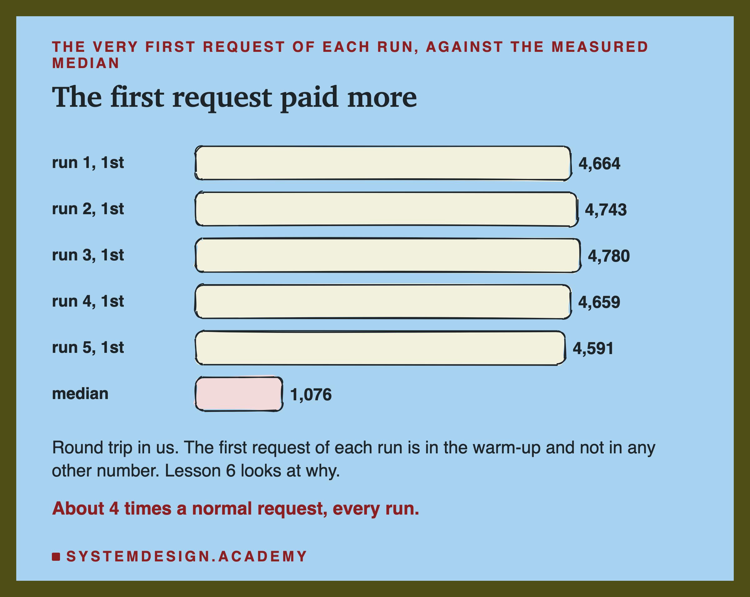
The first request of every run took between 4,591 and 4,780 microseconds. That is more than four times a normal request. It happened in all five runs, so it is not luck.

This is why the design sends a warm-up first. If I had counted the first requests, they would have pulled the tail up. The lesson would then mix two questions: what a normal request costs, and what the first one costs. The first one is the topic of lesson 6, cold starts, so here I only show it and move on.

Predict was the biggest step. But what part of predict is the model's real work? To get a first idea, I timed predict_proba alone in a fresh program on the box, with no web service around it. I label this a preview: lesson 4 measures it properly.

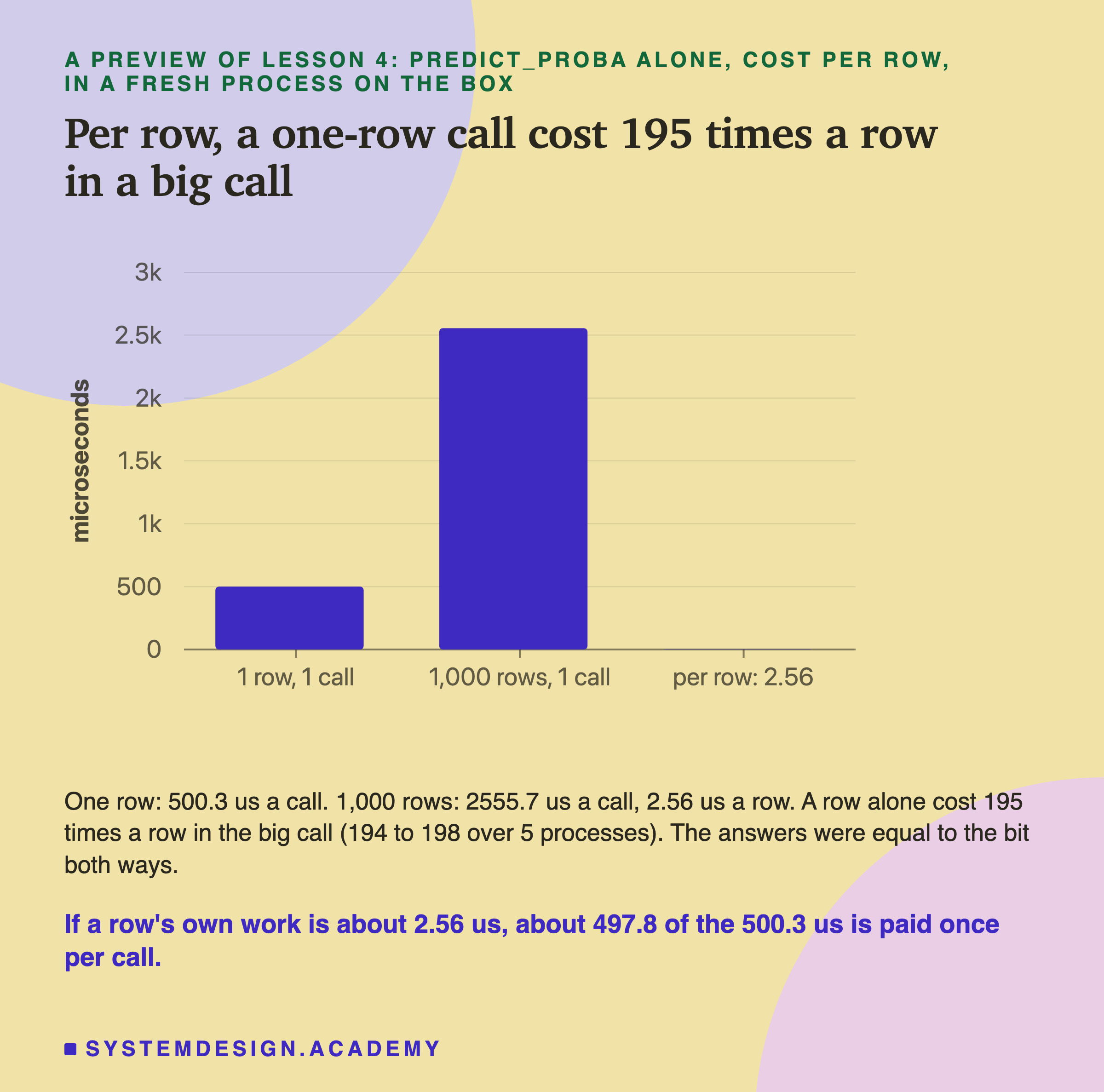
On one row, predict_proba took 500.3 microseconds a call. On 1,000 rows at once, it took 2,555.7 microseconds, which is 2.56 microseconds per row. So a row on its own cost about 195 times as much as a row inside the big call. The five fresh processes all gave between 194 and 198 times.

What does that mean? Suppose the real work for one row is about 2.56 microseconds. Then, in this preview, about 497.8 of the 500.3 microseconds are paid once for every call, whatever the number of rows. Some of it is likely scikit-learn checking the input before the trees run, but I did not time the parts of predict_proba separately. Lesson 4 asks whether sending rows together, called batching, is worth it for a service.

One more thing I noticed and did not explain: predict took 583.8 microseconds inside the service, but 500.3 here, alone. The rows are the same kind of data. One possible reason is the processor's caches, small fast memories next to the core. In the preview, predict ran 5,000 times in a row and its code and data stayed in the caches. In the service, the client, uvicorn and SQLite ran between two predicts, and they may push predict's data out, so each predict starts with a cold cache. I did not test that.

I wrote seven guesses into the lab before it ran. Here they are against the results.

1. "Inside the handler, predict is the largest step, larger than all the other steps together." Right: 583.8 microseconds against 72.6.

2. "The SQLite lookup takes under 50 microseconds at the median; parse and serialize each under 50 microseconds." Right: 34.5, 19.3 and 11.6.

3. "The time outside the handler is at least a third of the round trip, and the /noop round trip is at least half of the /score round trip's outside-the-handler part." Right: 37%, and 333.6 is 84% of 397.0.

4. "p99 is under 3x the median for the round trip on a quiet box." Right: 1,219.2 against 1,075.9.

5. "The five runs agree: each run's median round trip within 10% of the others." Right: they were within 0.5%.

6. "Preview: one row costs at least 50x the per-row cost of a 1,000-row call." Right: 195 times.

7. "Every returned score equals this Mac's score to the bit or within 1e-15." Right: the largest difference was 2.8e-17.

All seven were right, and that made me suspicious, because a clean result can mean the check is too easy. So I looked harder at the raw data, and that is how I found the two humps in the body read and run 0's slow tail. Neither was in my guesses.

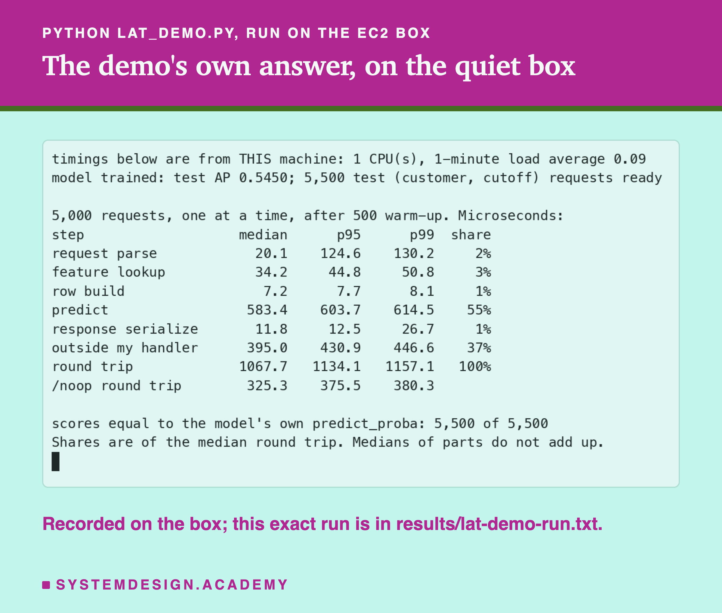
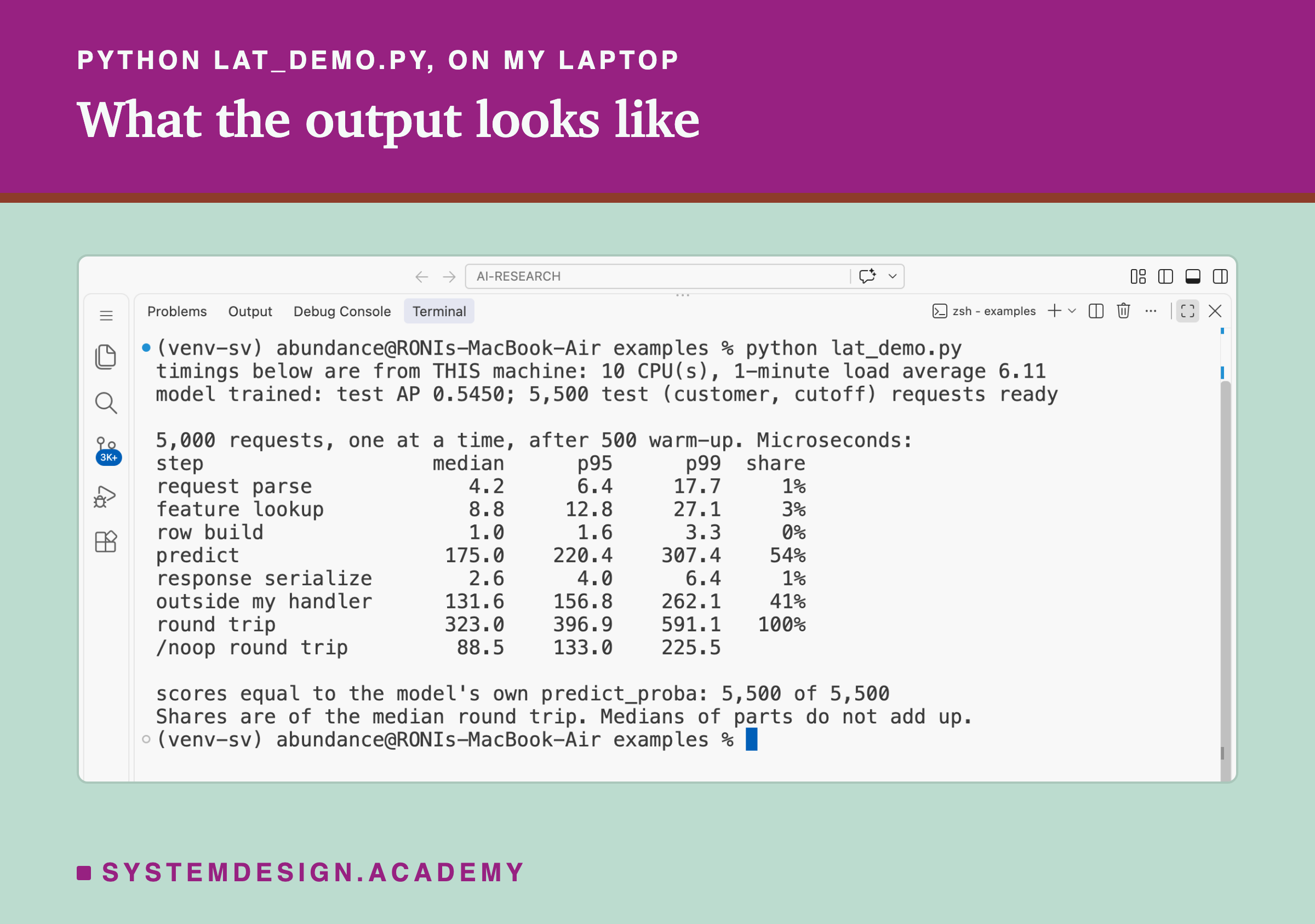
The full lab needs a rented box and five runs. I wrote a small demo, lat_demo.py, that builds the same service on your own computer and times it, in about a minute.

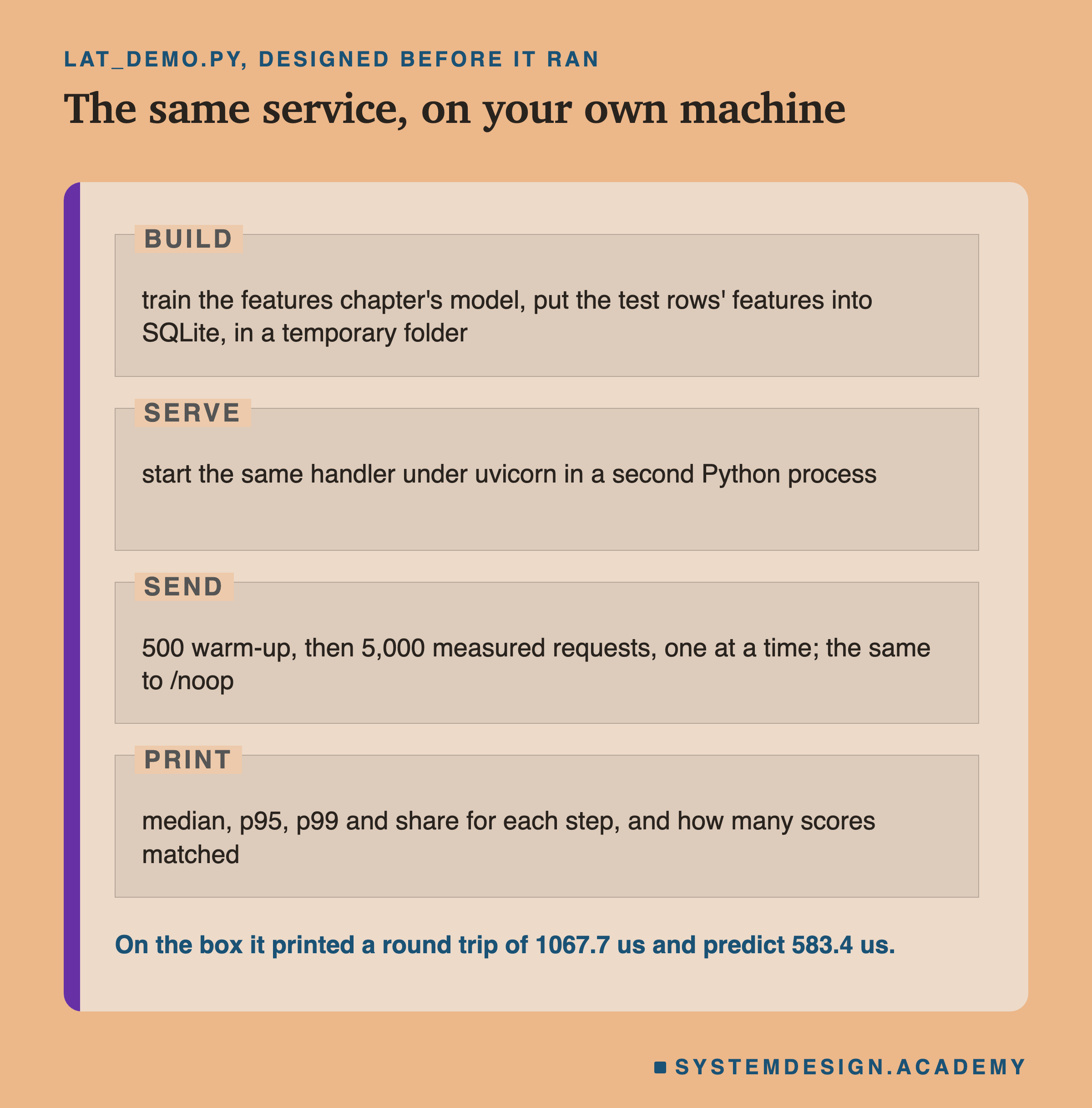
I wrote the demo's design into its docstring after the lab's design and before the demo first ran. It trains the model, puts the features into SQLite in a temporary folder, and starts the same handler in a second Python program. Then it sends 500 warm-up requests and 5,000 measured ones, and prints the table. After the main runs, I changed one printed line to fit the terminal. Later, a test run in an environment without uvicorn crashed with a long error. So I added a check of the packages, a wait for the service to answer, and one-line error messages. Nothing that is timed changed.

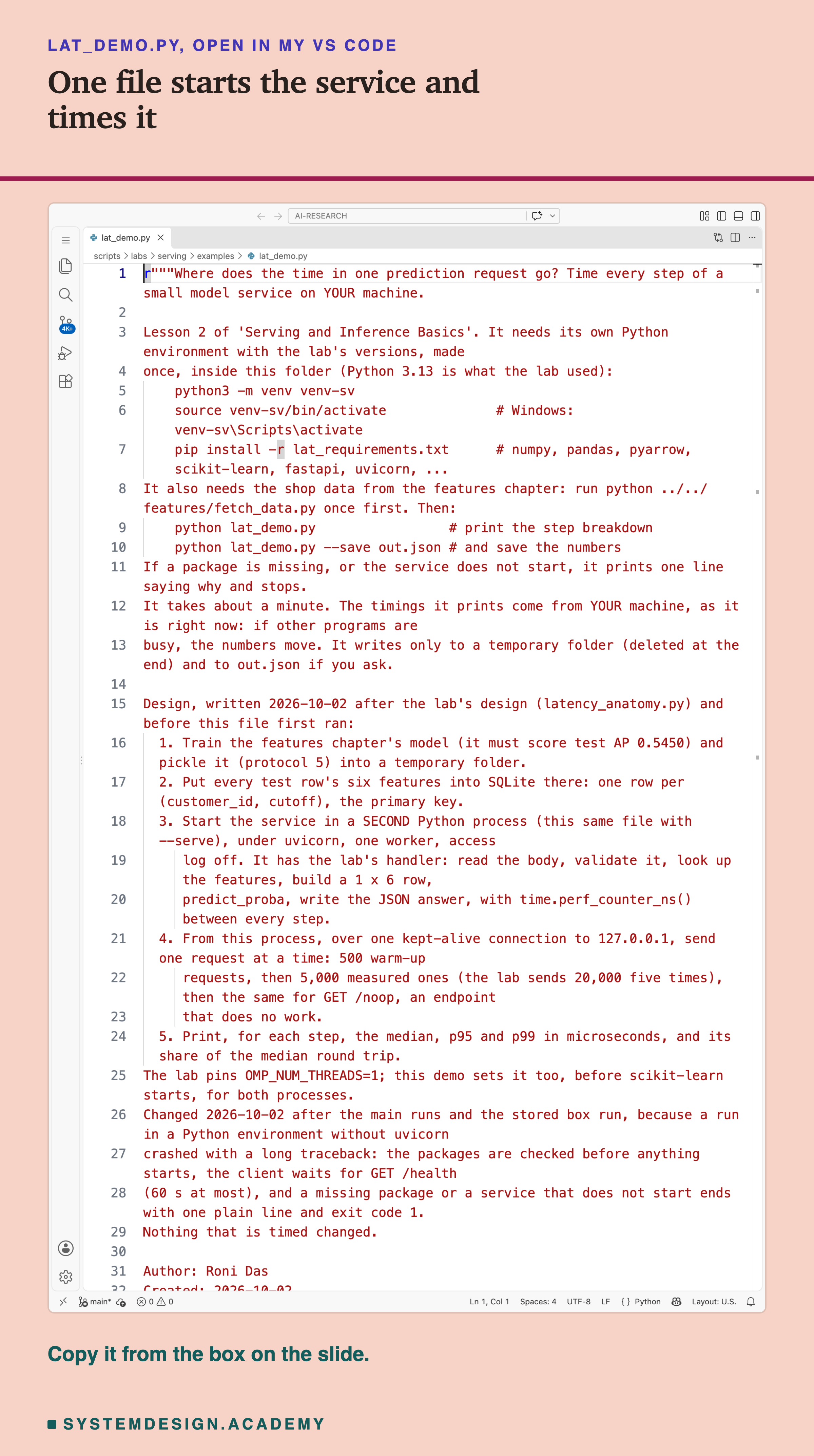
Before you run this lab. The demo needs its own Python environment with the same library versions as the lab's box. Make it once, inside the scripts/labs/serving/examples folder:

python3 -m venv venv-sv
source venv-sv/bin/activate        # on Windows: venv-sv\Scripts\activate
pip install -r lat_requirements.txt

The file lat_requirements.txt pins numpy, pandas, pyarrow, scikit-learn, FastAPI, uvicorn and the rest to the lab's versions. I used Python 3.13. Then run python ../../features/fetch_data.py once. It downloads the shop data, about 46 MB, and writes one cleaned file. Now run python lat_demo.py. It needs no GPU and no cloud account. If a package is missing, or the service does not start, it prints one line saying why and stops.

This box holds the real timings from the lab. It needs nothing but Python, so it runs in your browser. It has no model and no clock: it only looks up what the box measured.

Press Run. Then change STAT to "p99" and see which steps grow. Try RUN = 3 or RUN = 5 to see one run on its own. Set ROWS = 1000 to see the preview of lesson 4.

The report script writes this box from the lab's stored results, runs it with five settings, and checks that it prints the lab's numbers. Each # in a bar is 20 microseconds, so you can see predict's long bar next to the short ones.

The lab has one file that runs on my laptop and a few small files that run on the box.

latency_anatomy.py, on my laptop, does the parts that need no clock. prepare trains the features chapter's model and stops unless its test AP is exactly 0.5450. Then it writes three files: the model, the features of every test row, and the shuffled list of requests with the score my laptop's model gives for each. provision installs Python and the libraries on the box and copies the files there. run, preview and demo start the timed parts over ssh and copy the raw timings back. collect does the arithmetic, and teardown deletes the box, its key and its network rule, then checks they are gone.

lat_files/service.py is the service. Its handler reads the clock seven times and stores the readings in memory. The client fetches them from a third address, /timings, after the run, so the timings never travel inside a measured answer.

lat_files/client.py builds every request body before it starts. Then it sends them one at a time over one connection that stays open, and reads the clock just before sending and just after reading the answer.

lat_files/run_once.sh waits until the box is quiet, starts a fresh service, runs the client, stops the service, and records the load average and the CPU counters before and after. is the lesson 4 preview.

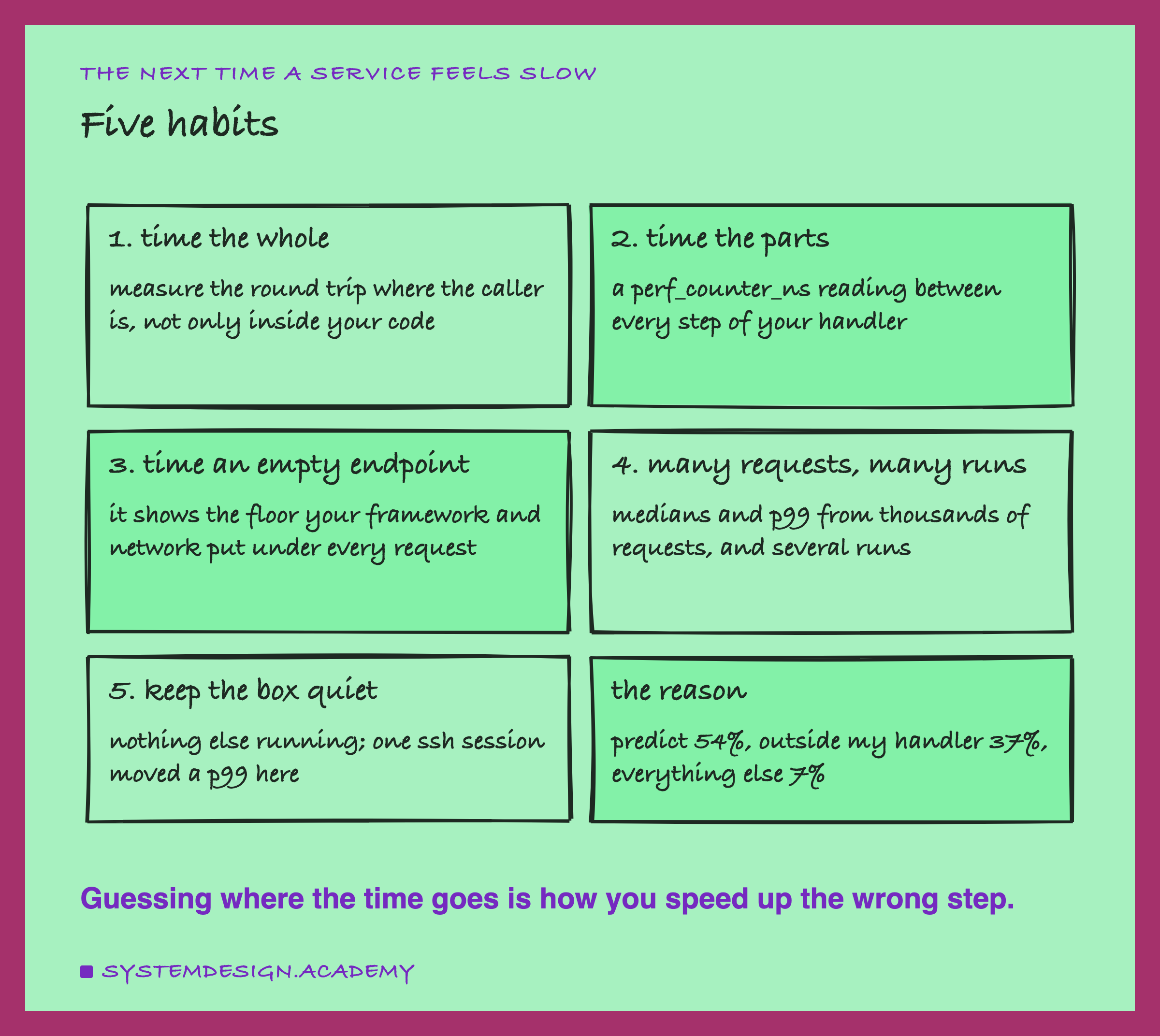
Here is the order I would use to look for the time in a slow service, using only what this lab did.

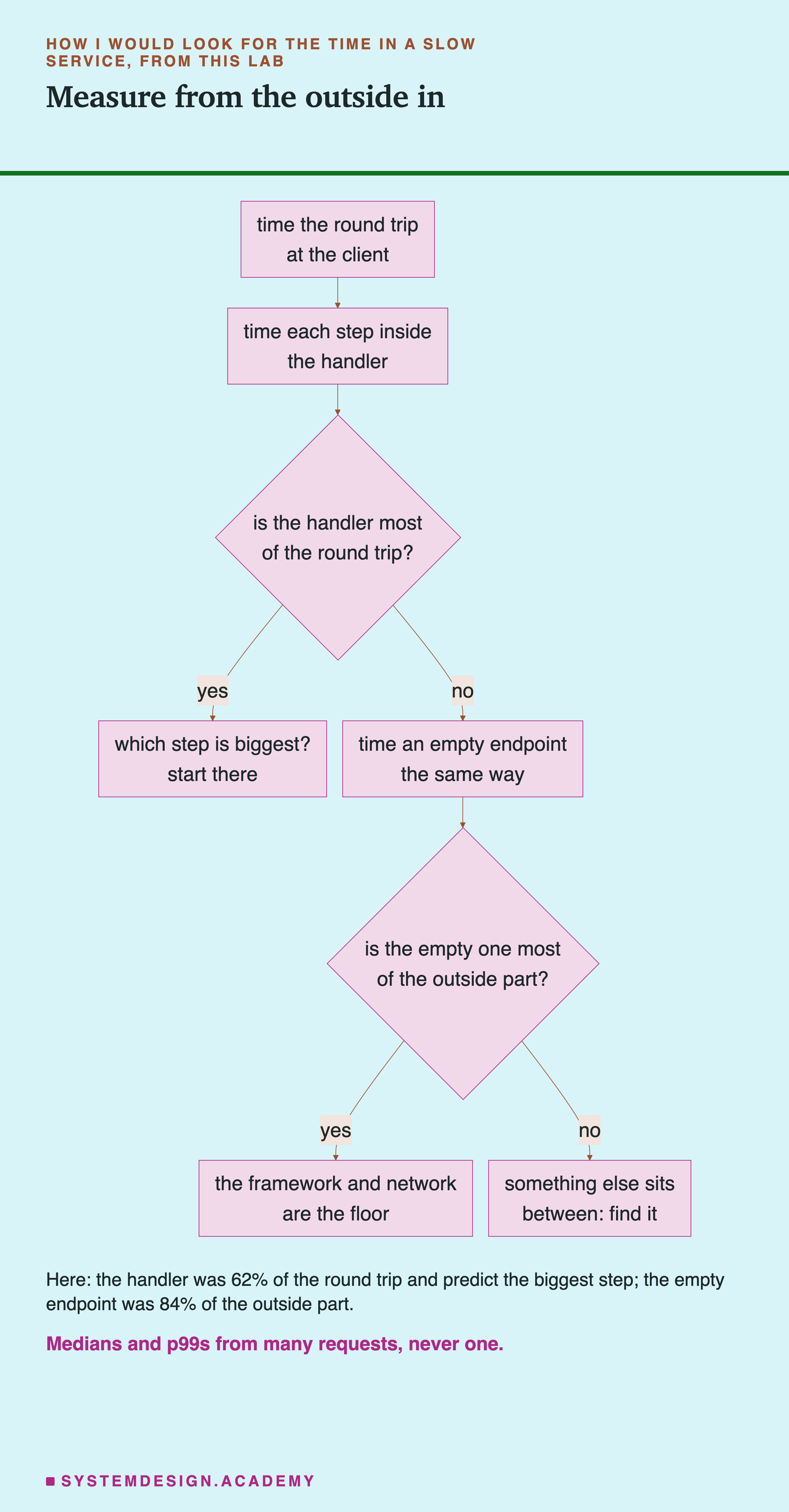
The chart starts from the outside, where the caller waits, and moves in one step at a time. Here are the same steps in words, each with the number from this lab behind it.

1. Time the round trip where the caller is. Inside your code you only see part of the wait. Here, 37% of the time was outside my handler.

2. Read the clock between every step of the handler. Use a precise clock, such as time.perf_counter_ns in Python, and keep the readings in memory, not in the answer.

3. If the handler is most of the time, start with its biggest step. Here predict was 54% of the round trip, and the four other steps together under 8%. Making the lookup twice as fast would have saved about 17 microseconds out of 1,076.

4. Time an endpoint that does nothing. Here it cost 333.6 microseconds. No change inside the handler can remove that.

5. Send many requests and repeat the run. Report the median and the p99, and how much the runs differ.

6. Keep the machine quiet, and check it. Here one ssh session was enough to move a p99.

Use step timings before you change anything. Here, without them, I would have guessed the database lookup was a big cost. It was 3.2% of the round trip.

Use an empty endpoint whenever the outside part is big. It tells you what the framework and the network cost on their own. If that floor is too high for your users, you need a different setup, not a faster handler.

Use many requests and several runs. One request tells you nothing: the first one here cost more than four times a normal one. One run can be spoiled, as run 0 was.

Do not time on a busy machine. My laptop's load is why every number here comes from a rented box. If you must time on a shared machine, record its load before and after, and say so.

Do not read these numbers as a law. They are one small tree model, one request at a time, on a quiet 1-core box. A large neural network would likely spend more of its time computing, and a busy service spends time in queues. Measure your own service in the same way rather than borrowing my shares.

Do not copy my handler as it is into a busy service. It is an async def, but it calls SQLite and predict_proba, which block. With one request at a time that changes nothing. With many requests at once, a blocking call inside an async def stops the whole event loop until it returns.

FastAPI's documentation says: "When you declare a path operation function with normal def instead of async def, it is run in an external threadpool that is then awaited, instead of being called directly (as it would block the server)." So write it as a plain def, or move the blocking calls off the event loop. Lessons 5 and 7 measure what this does under load.

Do not trust a timing with no check that the answers are right. Here every score was checked against my laptop's model. A fast service that returns wrong scores is not fast, it is broken.

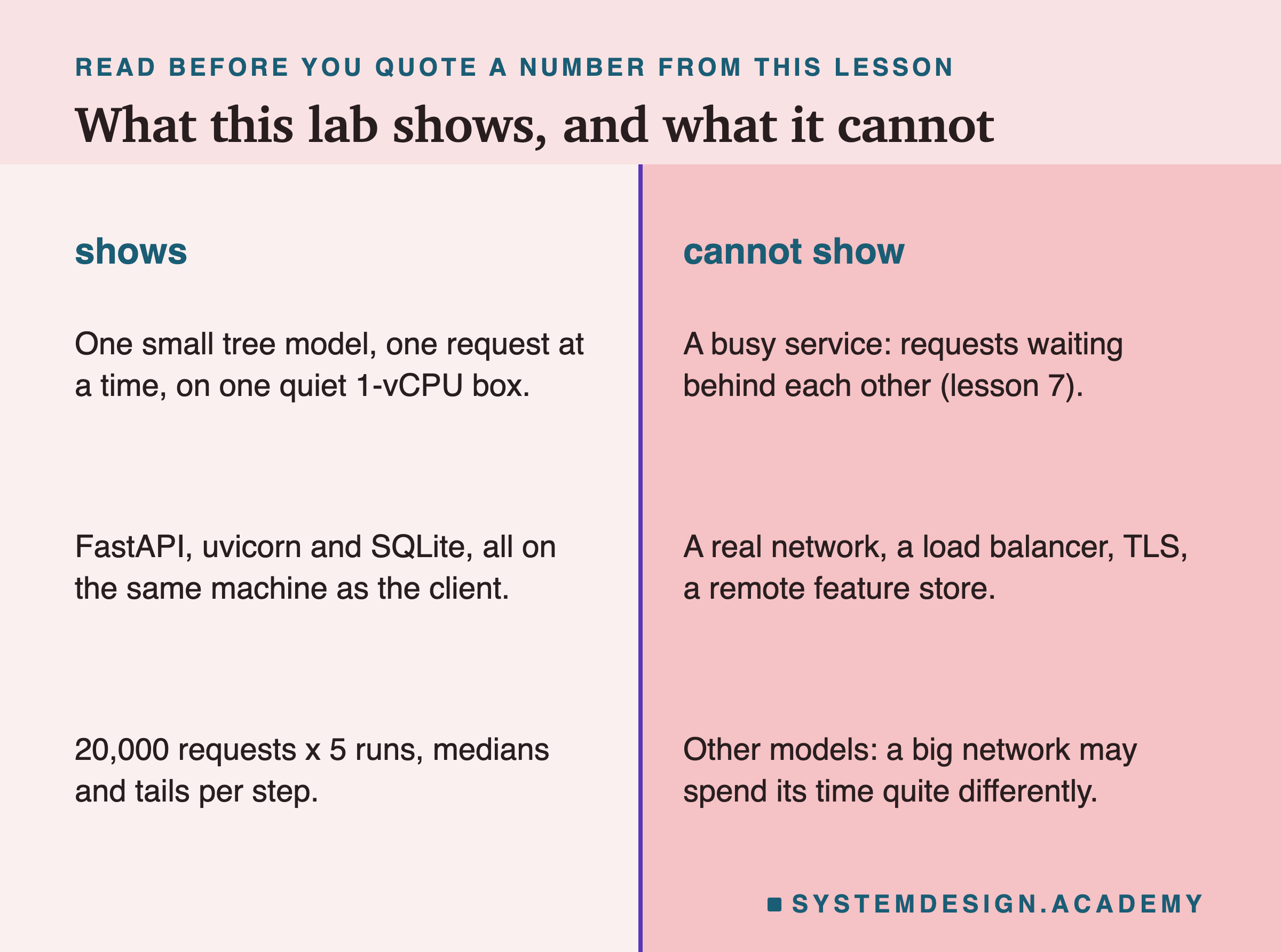
One box, one core. Everything here ran on one c7g.medium with one core, client and service together. On a machine with more cores, or with the client on another machine, the outside part would be different, and I did not measure that.

No real network. The requests used the loopback. A real network adds time for the distance, and a real service usually has TLS, the encryption behind https, and a load balancer in front. The survey lesson's request path includes them; this lab does not.

One request at a time. No request waited behind another. In a busy service, waiting is often the biggest cost. Lesson 7 measures it.

One model. The model is small and fast. A big model would spend more of each request in predict.

Labelled additions. The two humps, run 0's exclusion and run 5 were added after the first results, and the lab says so in its docstring. The demo's last printed line was reworded after the main runs.

If you take one thing to work on Monday, open the handler of a service you own and add a clock reading between every step. Store the readings, send a few thousand requests on a quiet machine, and look at the medians and the p99s. Then add an endpoint that does nothing, and time it too.

You may find, as I did, that the step you were worried about is small. A large part of the time may not be in your code at all.

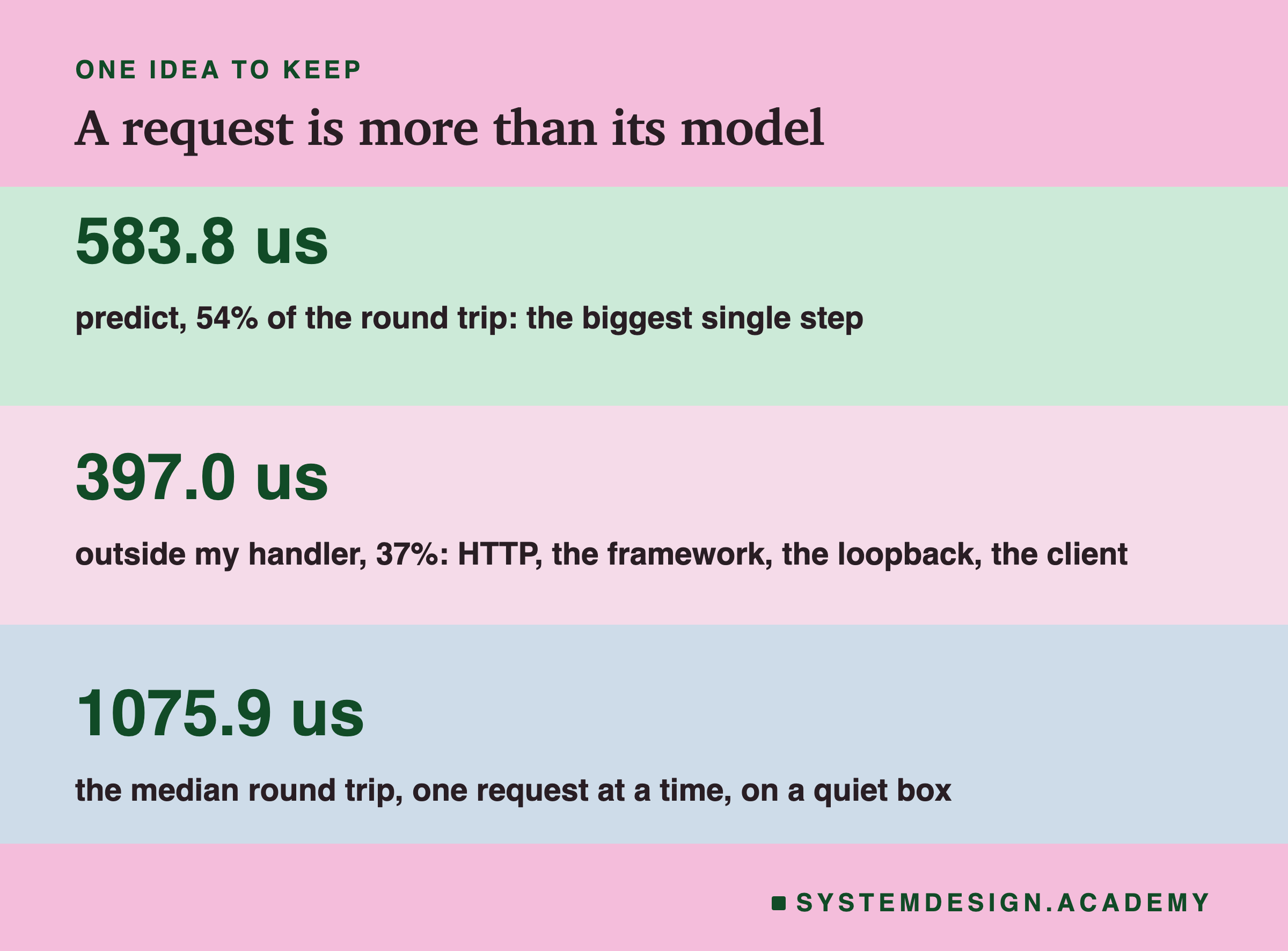
The one idea to keep: a prediction request is more than its model. Here the model was the biggest single step, a little over half of the time. But more than a third of the time was spent before and after my code, and an empty request already cost almost a third of a millisecond. Measure every step, from the caller's side and from inside, before you decide what to make faster.