Imagine a small school with a board by the front door. Every morning at seven, the caretaker looks out of the window and writes the day's weather on the board: "dry", or "rain". Parents read it when they drop their children off, and teachers read it at lunch to decide whether the children can play outside.

One day the caretaker writes "dry" at seven. At two in the afternoon it starts to rain hard. The board still says "dry". Nothing on the board looks wrong. It looks exactly like every other dry day, in the same handwriting, in the same place. A teacher reads it and sends thirty children out into the rain.

Now imagine a second problem. The school's thermometer was marked years ago, in the depth of winter, and whoever marked it wrote "normal" at a very cold point. Ever since, every reading shows "far above normal", in summer and in winter alike. That one is easy to spot: a board that says "far above normal" every single day is clearly broken, and someone will ask about it within a week.

Both problems come from the same thing: a stored piece of information that nobody updated. But the first one is quiet and the second one is loud. This lesson measures both kinds in a program that learns from examples, and asks which one does more harm before anyone notices.

This chapter follows one model through its life, on the same electricity data. Start with the dumbest model set the baselines. Same code, different model and picking the best of many looked at training. The promotion gate and canary and shadow looked at how a new model is judged and put live, and when to retrain asked how often to train it again.

All of those lessons treated the model as the thing that goes stale. This one looks at the pieces around it. The course's lesson on training pipelines and orchestration has a slide called "Skip the Work You Already Did: Caching". It explains in words how a pipeline saves the output of a step and reuses it when nothing changed. I will not repeat it. This lesson measures what happens when a saved piece is reused after something did change.

The previous chapter measured two close relatives. Train/serve skew computed one input two different ways, and failing silently tested which simple checks catch a broken input before the right answers arrive. Here the input is computed the right way, by the right code. It is just old. I reuse that lesson's checks later on, on these new inputs.

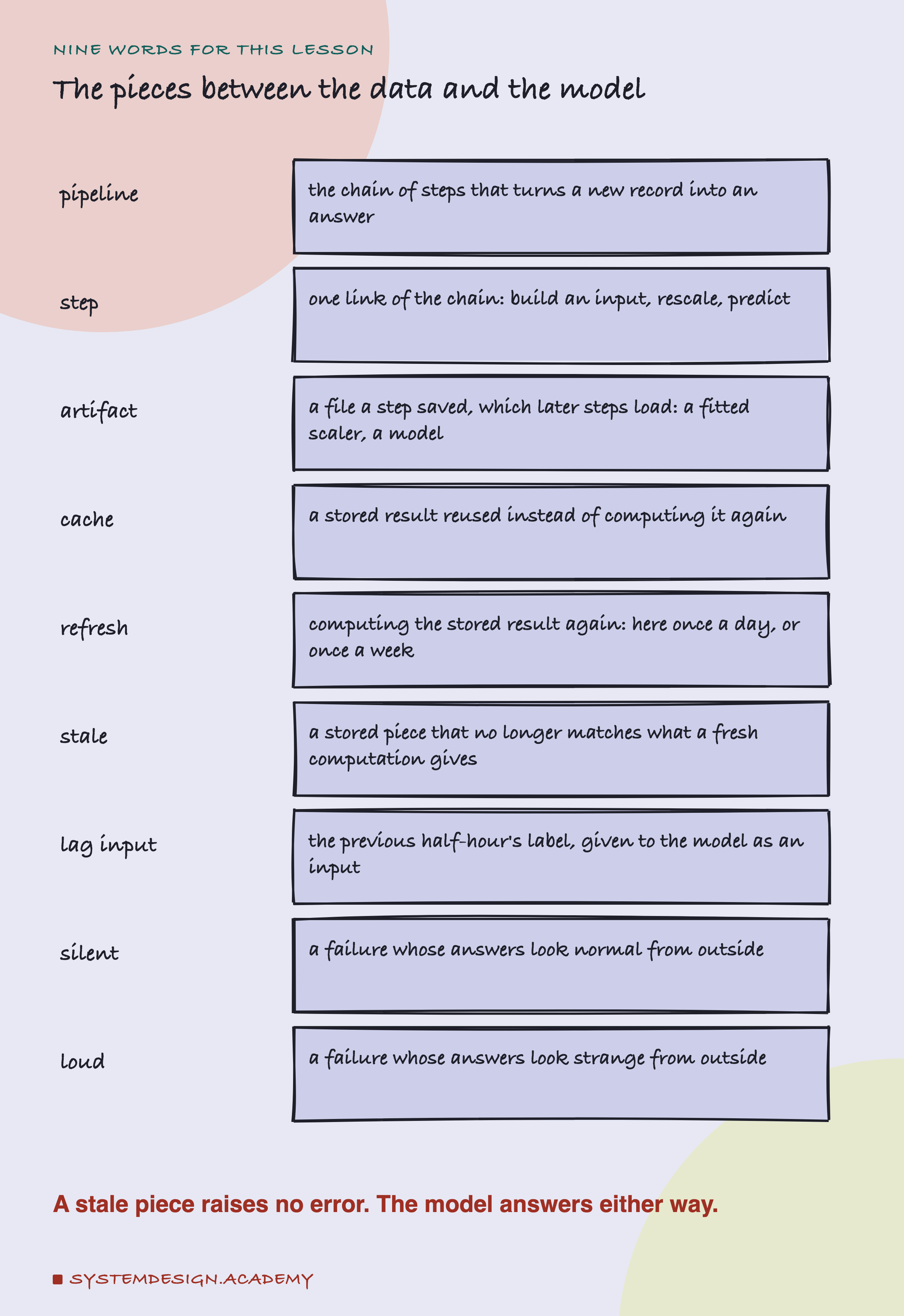
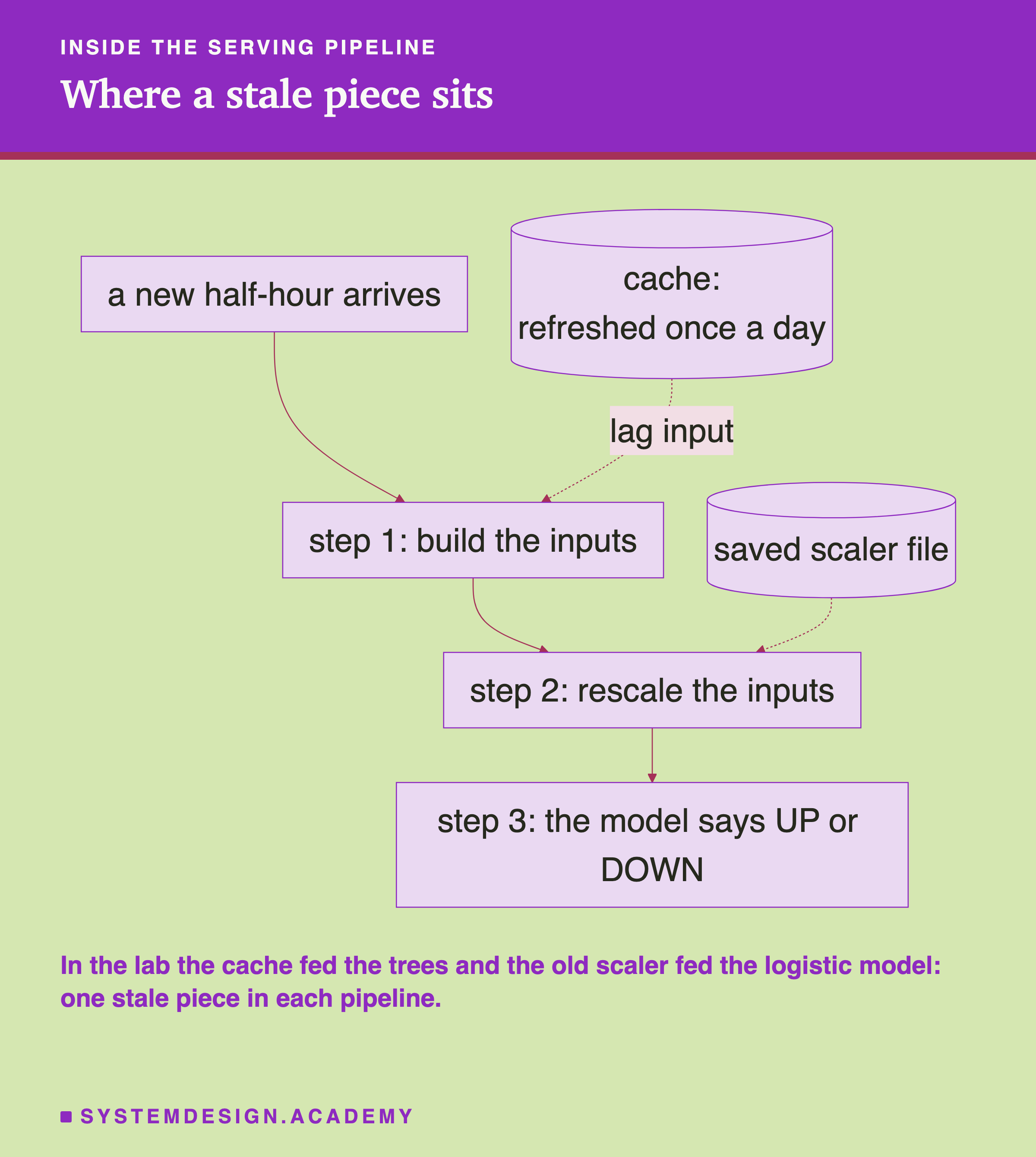
A pipeline is the chain of steps that turns a new record into an answer. Each link is a step: build the inputs, rescale them, ask the model. Many steps save what they made so that later steps, or later runs, can load it. A saved file like that is called an artifact. A fitted scaler is an artifact, and so is the trained model itself.

A cache is a stored result that is reused instead of being computed again. Computing it again is a refresh. A cache saves time and money, and it is safe as long as the stored result is still what a fresh computation would give. When it is not, the stored piece is stale.

This lab caches one input, the lag input: the label of the previous half-hour, which lesson 1 added to the trees to make its best model. The label is the right answer for a row: here, whether the price went UP or DOWN against its average over the last 24 hours. Accuracy is the share of rows a model got right, and a point is one hundredth of accuracy.

Last, two words for how a failure looks from outside. A failure is silent when the model's answers look normal: the same mix of UP and DOWN, nothing strange in any chart of the outputs. It is loud when the answers themselves look strange.

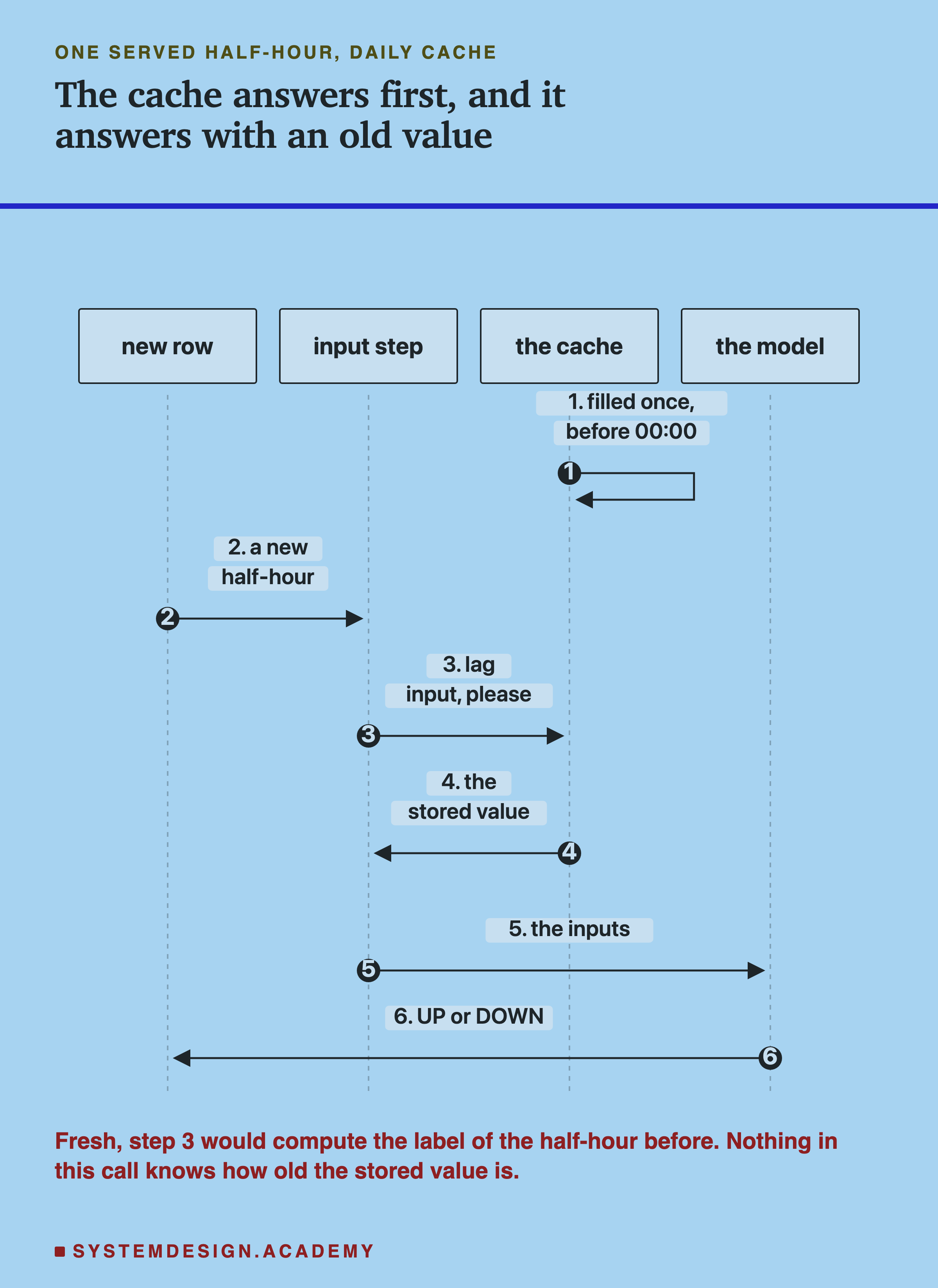
The lag input changes every half-hour. A fresh pipeline looks up the previous half-hour's label each time a new row arrives. A cached pipeline looks it up once, stores it, and serves the stored value until the next refresh. Here is a real day from the lab's test, sketched, with the cache filled once a day just before midnight.

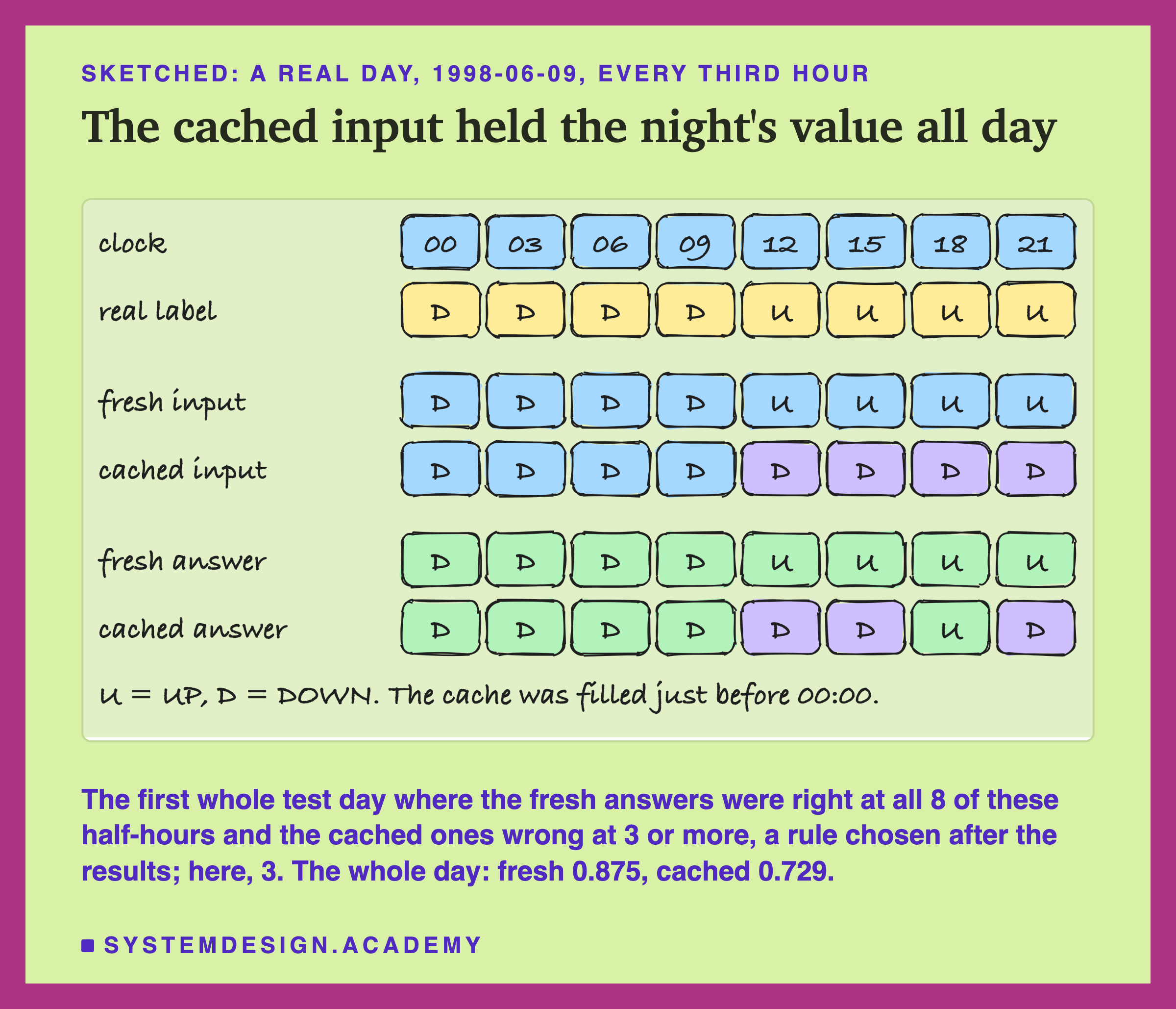
On this day the price was DOWN through the night and morning and turned UP around midday. The fresh input followed it: once the price turned, the previous half-hour's label was UP, and the model said UP. The cached input still held the label of the last half-hour of the day before, which was DOWN. It went on saying DOWN all afternoon, and the model, which leans heavily on this input, followed it for most of the afternoon. Over the whole day the fresh input scored 0.875 and the cached one 0.729.

Nothing in the pipeline raised an error. The cached value was a perfectly normal label, 0 or 1, of the same type and in the same place as the fresh one. The only thing wrong with it was its age.

Why would anyone cache an input like this at all? Because computing inputs fresh has a cost. In a real system the previous label might live in another database, owned by another team, and looking it up for every request adds time to every answer and load on that database. A popular pattern is to compute inputs in a batch job, once a night, and store them where the serving code can read them quickly. That design is sensible for inputs that change slowly. The trouble starts when the same pattern is used for an input that changes every half-hour, and nobody measures what the delay costs. That is exactly the choice this lab makes on purpose, so its cost can be counted. I picked this day with a rule I wrote after seeing the results, so it shows the mechanism clearly; it is not a typical day, and the averages come on the next slides.

I wrote the lab's design at the top of its file, stale_lab.py, before it ran. The dated record is in the chapter plan (2026-09-29, "STALE LAB (batch 7) designed before running").

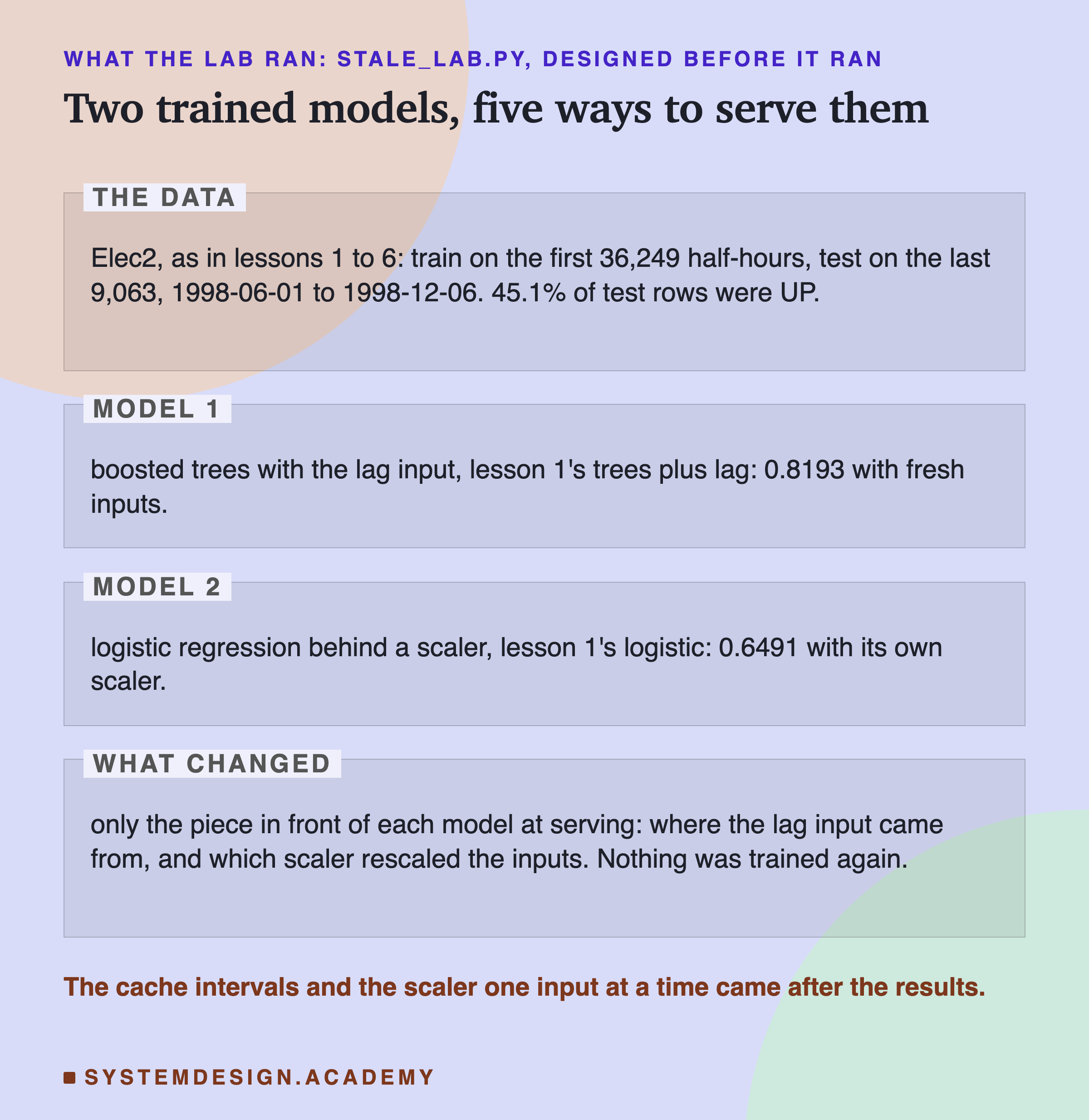
The data is Elec2 again: 45,312 half-hours of the New South Wales electricity market, May 1996 to December 1998, in time order. The models learn from the first 36,249 rows and are tested on the last 9,063, from 1 June to 6 December 1998, the same split as lesson 1.

The two models are also lesson 1's. The first is the boosted trees with the lag input: many small trees of yes-or-no questions, built one after another. The second is logistic regression, which adds up a weight for each input and turns the sum into UP or DOWN. Logistic regression needs its inputs on a similar scale, so a scaler sits in front of it. A scaler learns each input's average and spread from the training rows, and then standardises every new row: it subtracts the average and divides by the spread, so a value of 0 means "the training average" and 1 means "one spread above it". The fitted scaler is an artifact: a small saved file with two numbers per input.

Here is what the lab stored in results/stale.json.

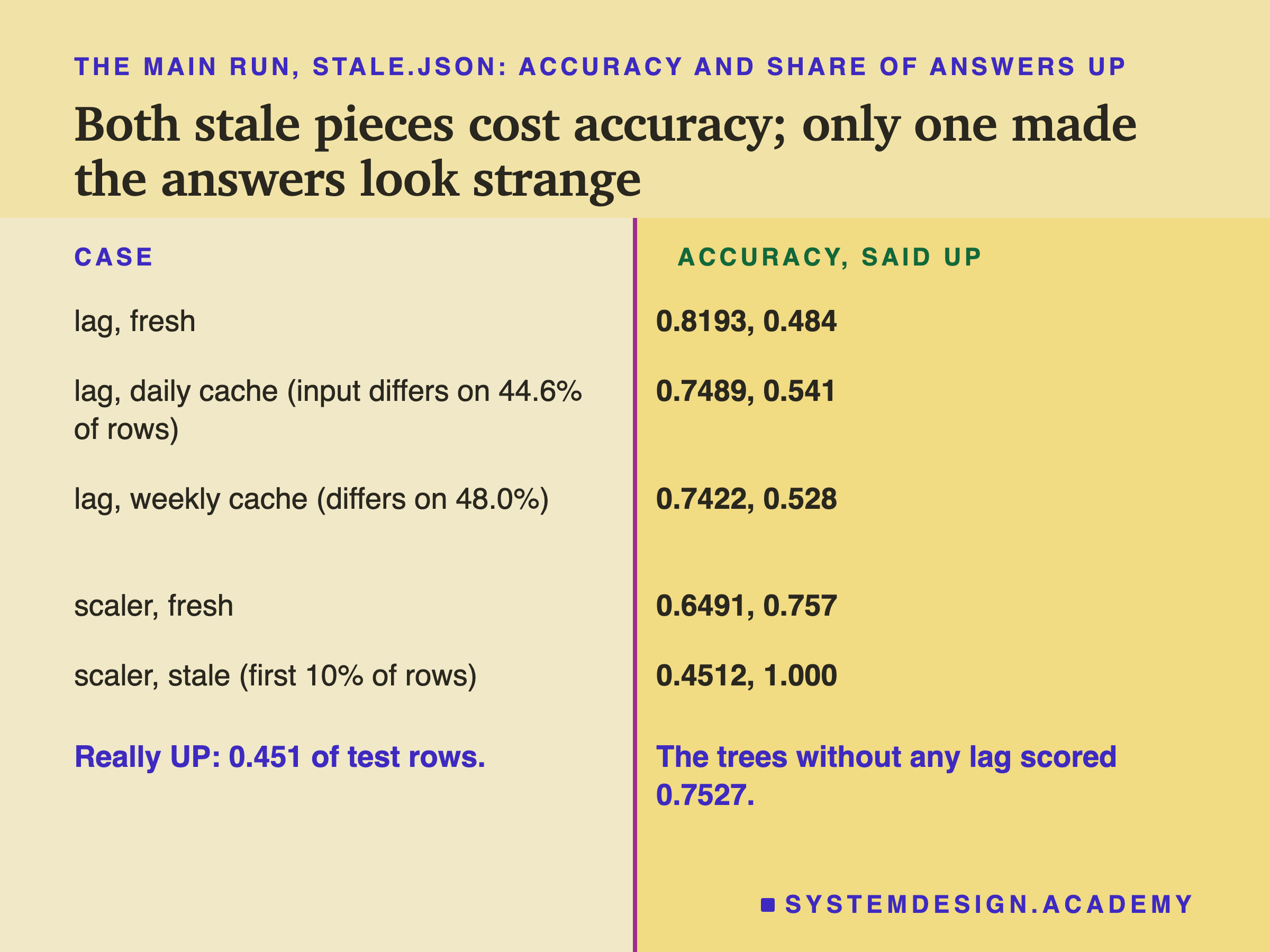
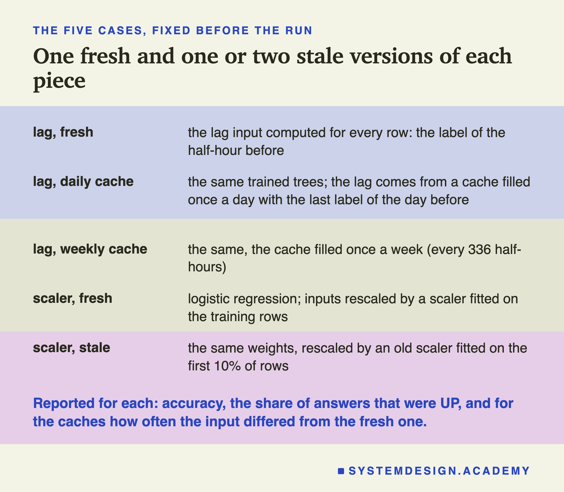
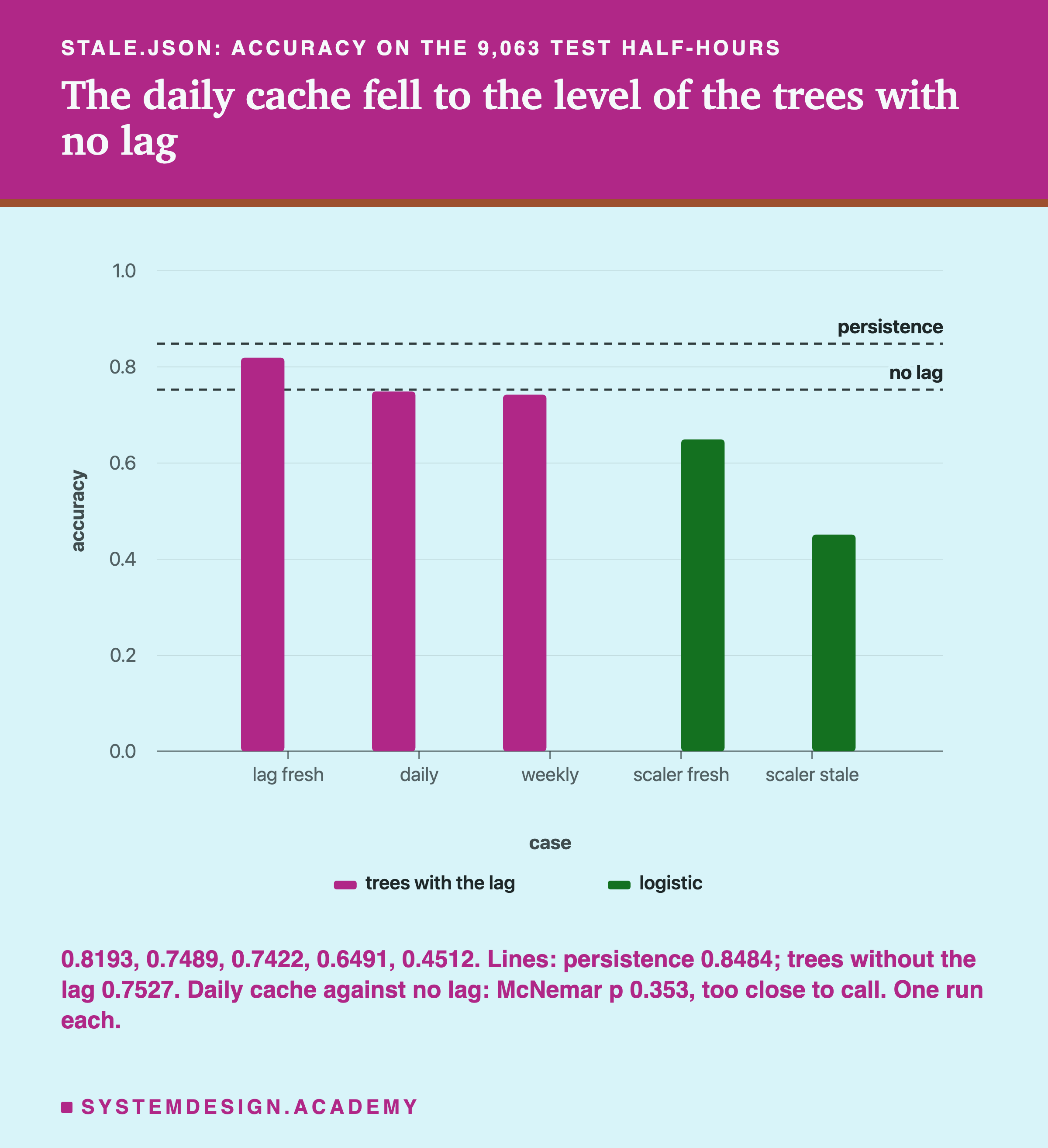
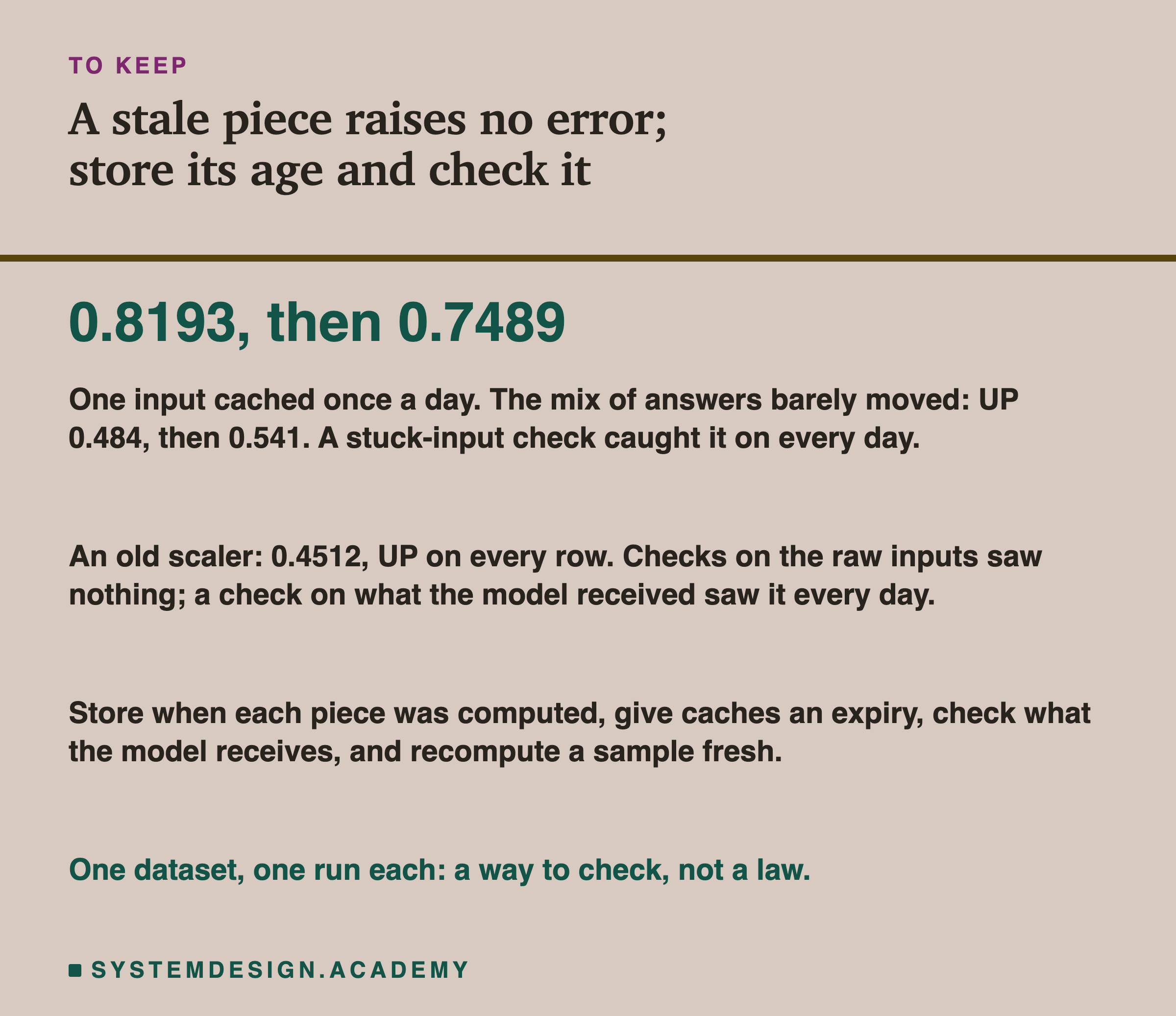
The daily cache cost 7.04 points: accuracy fell from 0.8193 to 0.7489. The cached input differed from the fresh one on 44.6% of test rows. The weekly cache cost a little more, 0.7422, with the input different on 48.0% of rows.

Now compare those with lesson 1's trees without any lag input, which scored 0.7527 on the same rows. The daily cache landed about the same as trees that never had the lag: 0.7489 against 0.7527, a 0.39-point gap in one run, too small to call. After the results I compared the two row by row. The cached-lag trees were right where the no-lag trees were wrong on 652 rows, and the reverse on 687; McNemar's test from lesson 4, counting only those rows, gives an exact two-sided p of 0.353, so the gap cannot be told apart from luck. The weekly cache, 0.7422, I did not test. So a day-old lag threw away all of what the lag had added, 7.04 points, and left the trees roughly where they would be without it. One possible reason, which is my reading and not a separate measurement: the trees had learned to trust that input a great deal, because a fresh lag is a very good guide on this data, and a stale one sent them the wrong way as often as it helped.

Persistence, the dashed line at 0.8484 on the chart below, is lesson 1's rule that simply copies the previous half-hour's label. It is a rule, not a model, and no model in this chapter has beaten it on this split.

Accuracy needs the right answers, and in many systems those arrive late or never. So the first question a team can ask, before any label arrives, is whether the model's answers look normal. The simplest measure of that is the output mix: the share of answers that were UP.

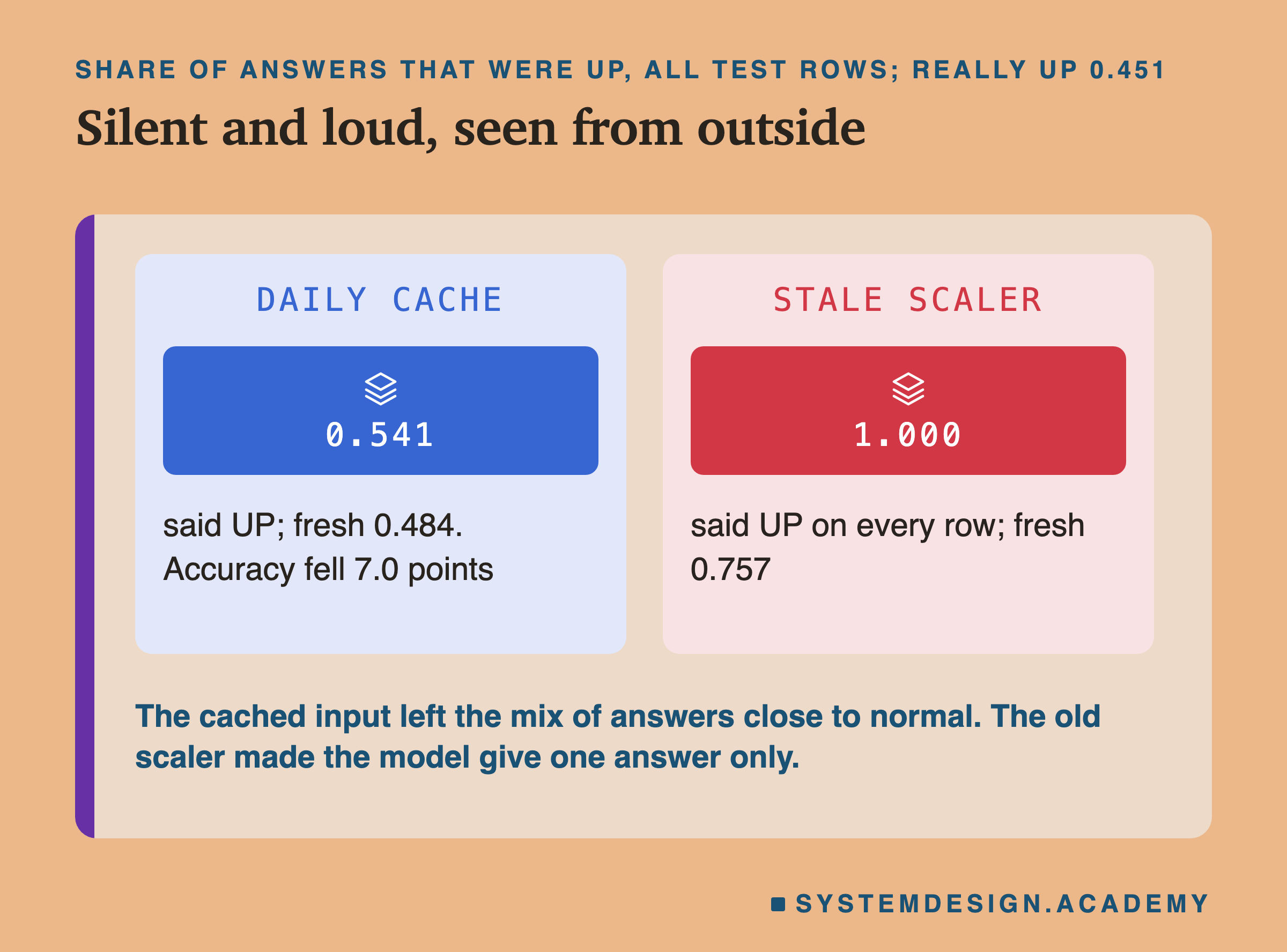
With the daily cache, the trees said UP on 0.541 of rows, against 0.484 with the fresh input and 0.451 in reality. That is a shift, but a small one, and the fresh model was itself 0.033 away from reality. Nobody looking at this number without the fresh one beside it would suspect anything. With the stale scaler, the logistic model said UP on every row. Its fresh version already said UP too often, 0.757, but "every row, every day" is a different kind of number.

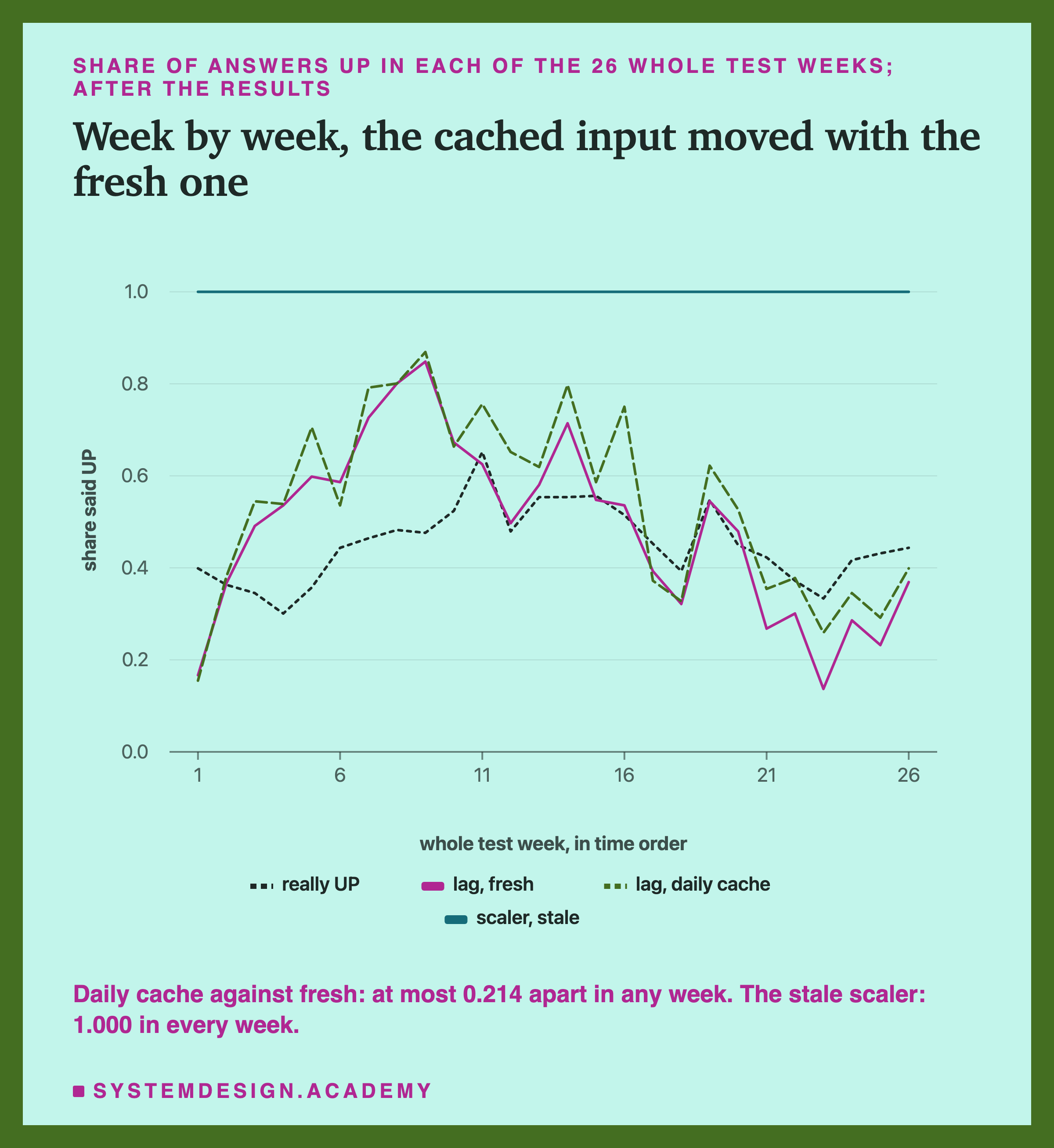
Week by week, which I measured after the results, the cached input's line rose and fell with the fresh one. In most weeks it was a little higher, and in the worst week the two were 0.214 apart. But the fresh line itself swings from 0.14 to 0.85 across the season, so a gap of that size hides inside the ordinary movement. The stale scaler's line is flat at 1.000, week after week.

So, from outside, the daily cache was silent and the stale scaler was loud. That is the most important point of this lesson: the silent failure cost 7 points of accuracy and looked normal, and a silent failure can run for months, because nothing makes anyone look. The loud one was far worse per row, but a model that says UP every day for a week is the kind of thing a person notices. I will show on a later slide that "notices" depends on which check you run, because the obvious daily check missed it too.

A cached input can only change an answer when the cached value differs from the fresh one. I measured this after the results, and it holds exactly: on every row where the two were equal, the model received the same row and gave the same answer.

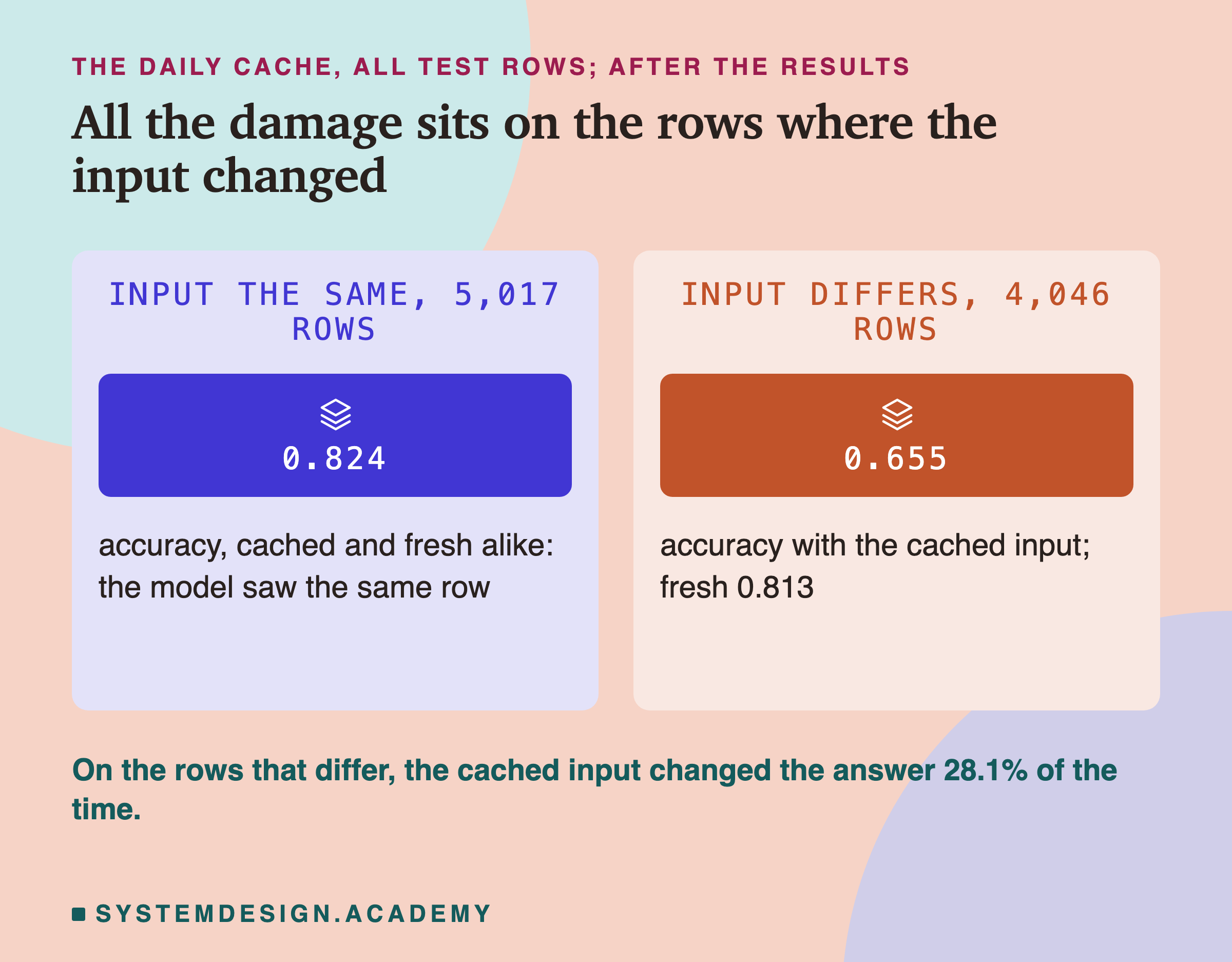
The cached input equalled the fresh one on 5,017 rows, and both scored 0.824 there. On the other 4,046 rows, the fresh input scored 0.813 and the cached one 0.655. On those rows the cached input changed the model's answer 28.1% of the time. That is the whole 7-point loss, concentrated on under half the rows.

A stale value fits best just after the refresh, so I expected the damage to grow through the day as the cached value got older. I measured it after the results, in blocks of three hours. As in lesson 1, the data does not say whether the first half-hour of a day starts at midnight, so I count it as 00:00; the clock times may be half an hour early.

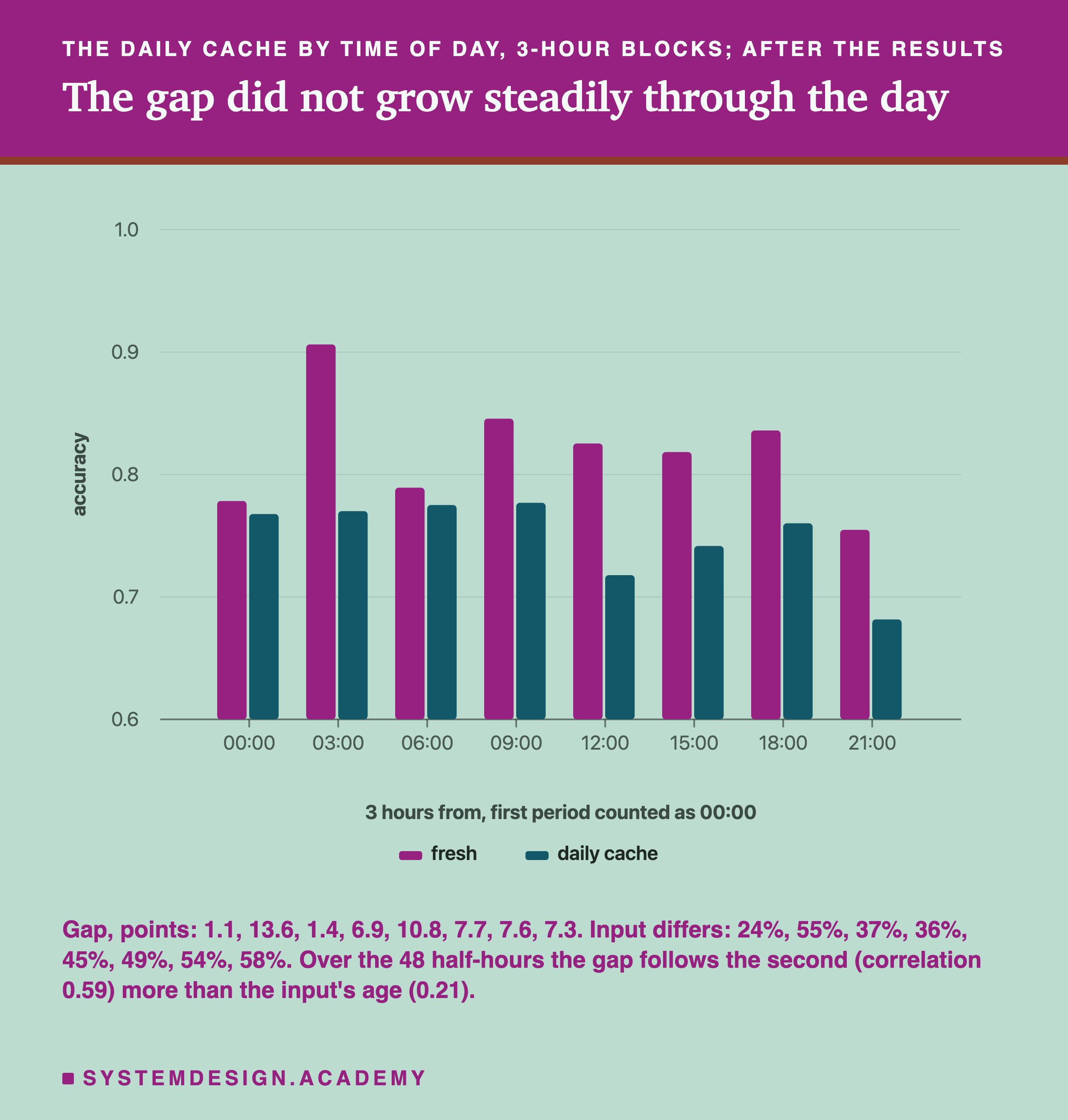
It did not grow steadily. The first three hours after the refresh lost only 1.1 points, as expected. But the next three hours, 03:00 to 06:00, lost 13.6 points, the most of any block, and 06:00 to 09:00 lost only 1.4. In this data the gap followed how often the cached value differed from the fresh one more closely than its age, and how often it differed follows the shape of the day's prices. From 03:00 to 06:00 the cached value, the label from late in the evening, differed from the fresh one on 55% of rows; from 06:00 to 09:00 on only 37%. Across the 48 half-hours of the day, the gap had a correlation of 0.59 with how often the input differed, and only 0.21 with the input's age. (A correlation of 1 means two numbers rise and fall together; 0 means no link.) Why the evening's label happens to match the morning better than the small hours is a question about this market's daily rhythm that I did not study.

Why did the old scaler make the model say UP on every row? After the results, I looked at the numbers the model actually received: every input, standardised by the old scaler, on every test row, next to the same inputs standardised by the training scaler on the training rows.

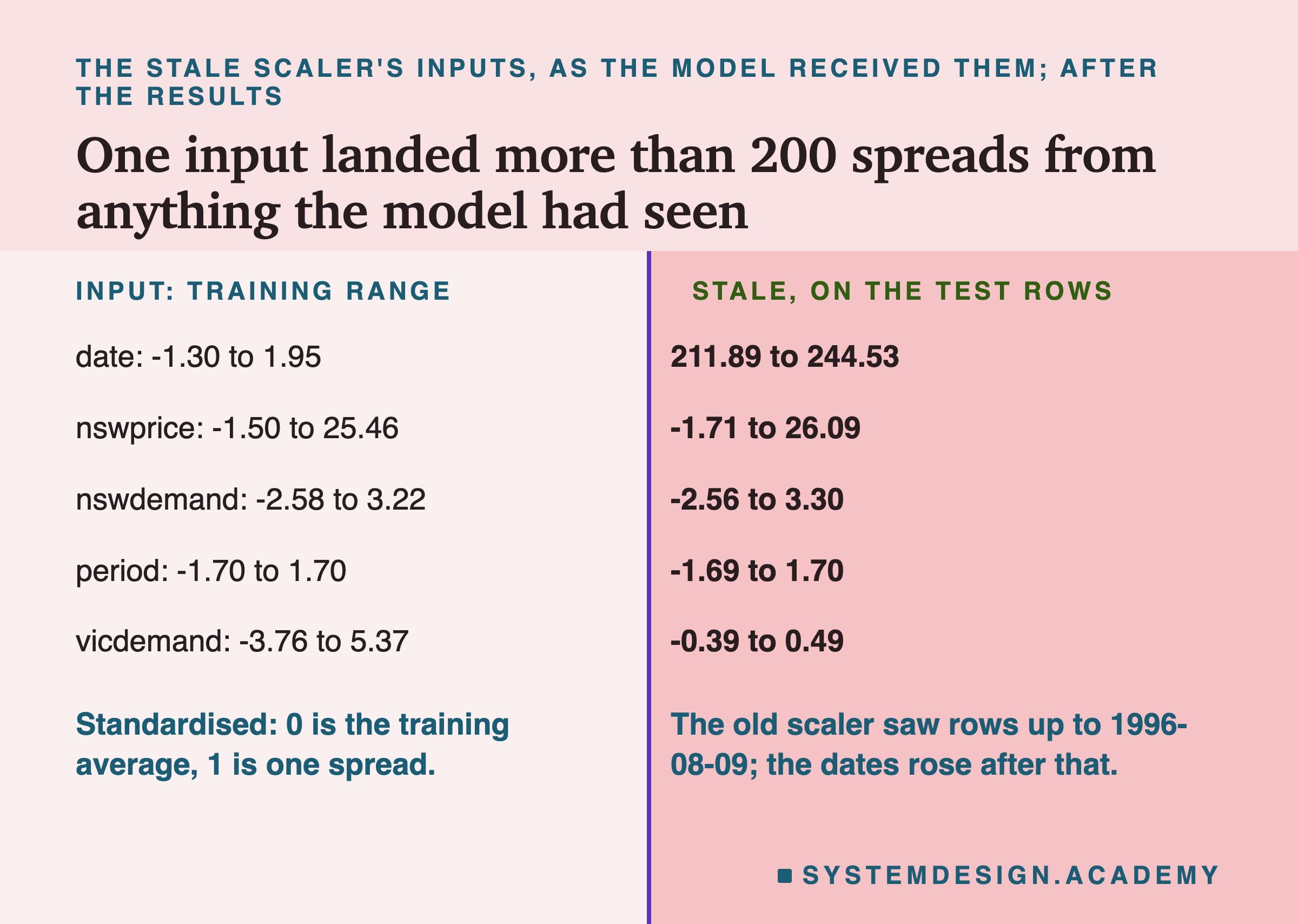
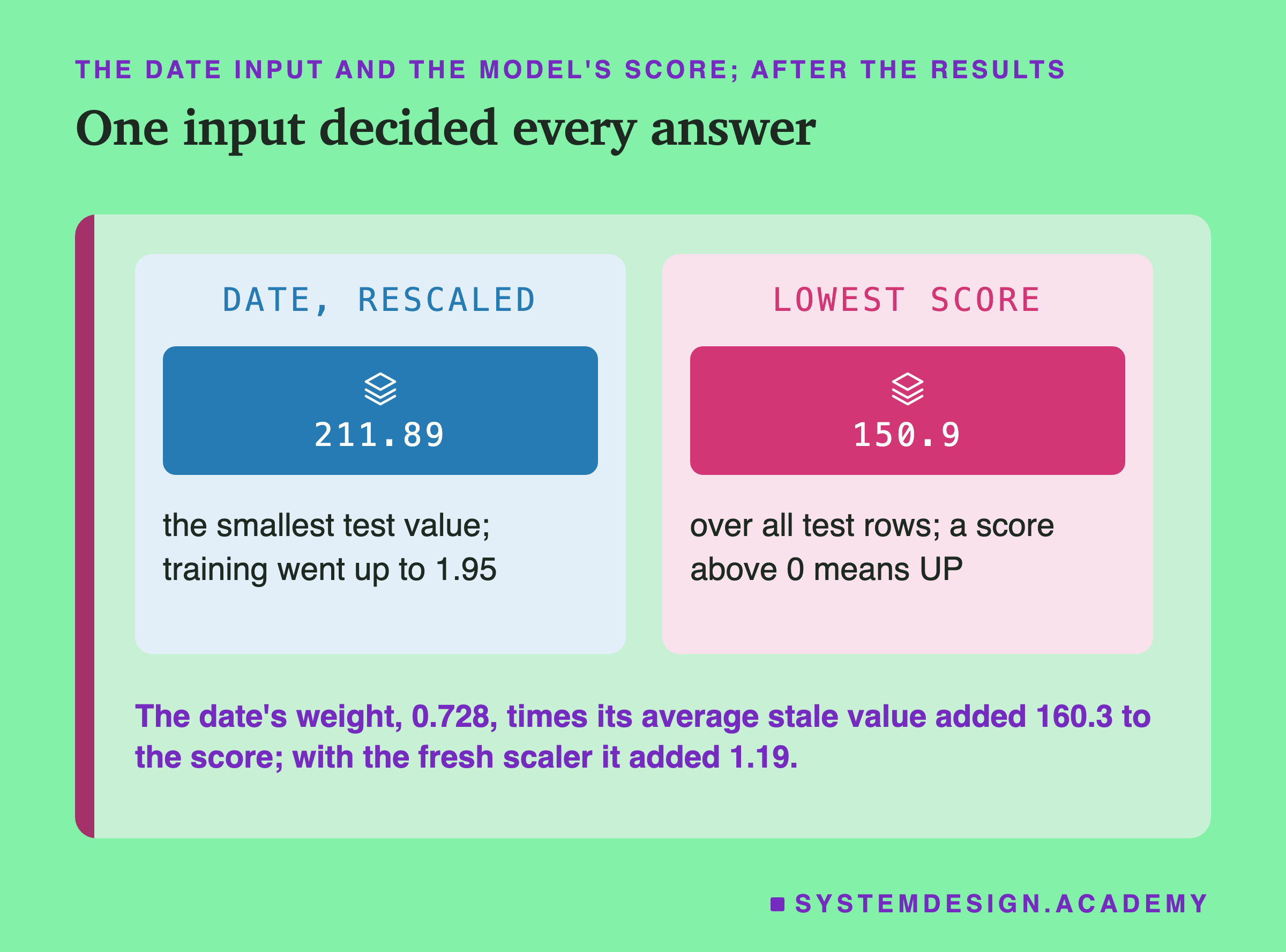
One input stands out. The date column in Elec2 is a number that mostly grows from 0 to 1 over the whole data (it steps back a few times, as lesson 6 noted). The old scaler had only seen the first 10% of the rows, whose dates ran from 0 to about 0.013, so it learned a tiny average and a tiny spread. The test rows' dates, around 0.87 to 1.0, came out as 211.89 to 244.53 spreads above its average. During training the model had never seen this input above 1.95.

Most other inputs landed close to their training range, because prices and demand in 1996 were not so different from 1998. Three inputs, vicprice, vicdemand and transfer, did something odd: in those first rows they held a single value, as the Victorian data in Elec2 begins later. A scaler cannot divide by a spread of zero, so scikit-learn set their spread to 1, and they came out squeezed near 0. Their weights in the model are small, so they did little here.

The previous chapter's lesson failing silently built simple checks that need no right answers and run once a day. After the results, I ran the same kinds of check on these inputs and outputs, one batch per whole test day, 188 days in all. None of them was tuned for this lab, and I wrote their exact rules knowing the results, so read this as a demonstration, not a fair trial. A range check fires when any input is below the lowest or above the highest value that input had in training. An unseen value check fires when an input that takes a few fixed values, such as the weekday or the lag, holds a value training never had. A zeros check fires when the day's share of inputs that are exactly 0 is more than 0.30 above the training share, the way a missing value filled with 0 would look.

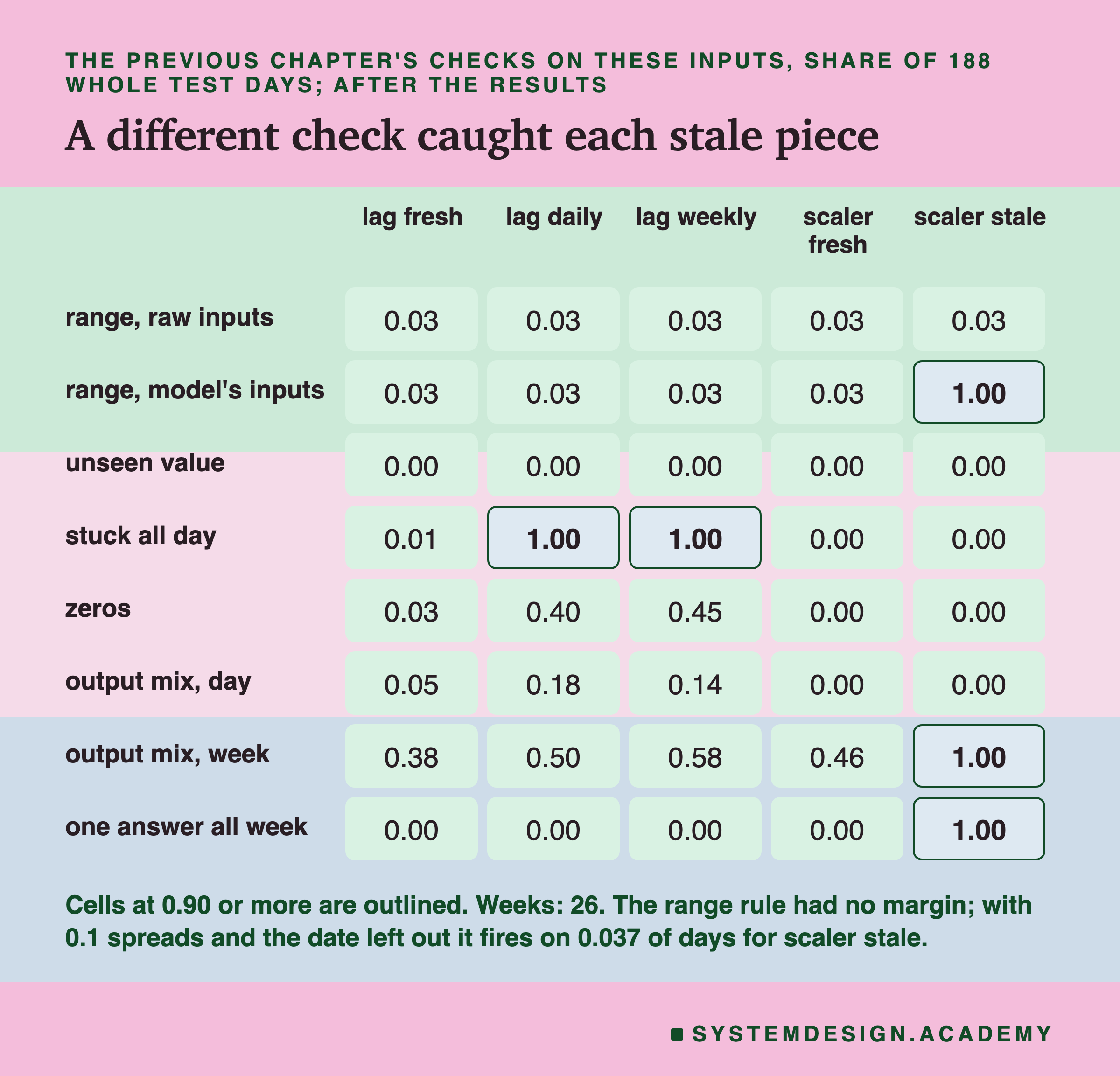
The daily cache was caught by the stuck check on every day. A stuck check fires when an input that normally moves within a day holds one single value all day. A cached lag does exactly that: it holds the night's value until the next refresh. With the fresh input, the lag held one value all day on 1 of 188 test days and 0.7% of training days, so the check is also quiet when nothing is wrong. The output checks were much weaker: the daily output mix fired on 18% of days with the cache against 5% without it, and the weekly one on 50% against 38%. Those checks fire often on the fresh model too, so they cannot tell you which days are broken.

The stale scaler was caught only by checks on what the model received. The raw inputs were untouched: the old scaler sits after them. So range, unseen, stuck and zeros on the raw inputs fired exactly as often as with the fresh scaler. The range check on the standardised inputs, the numbers the model really got, fired on all 188 days. But as I wrote it, the rule had no margin, and that matters: the period input crossed its training range by 0.003 spreads on every day, so even without the date the check would have fired every day. I measured the rule with margins after the review of this lesson. Leaving the date out, a margin of 0.01, 0.1 and 0.5 spreads made it fire on 0.197, 0.037 and 0.005 of days; with the date kept in, on every day at every margin, because the date was over 200 spreads outside. So with any sensible margin, only the date trips it, and it trips it on every day.

The main run tested a day and a week. A real team would ask a practical question: if we must cache, how often must we refresh? I designed a follow-up after seeing the main results and wrote its design into the lab file's followup mode before it ran. It served the same trees with the lag cached for 1, 2, 6, 12, 24, 48 and 336 half-hours. A cache of 1 half-hour is the fresh input, and 48 and 336 repeat the main run; both had to come back exactly, and they did. Its results are in results/stale_followup.json.

A cache refreshed every hour scored 0.8121, 0.72 points below fresh. Every 3 hours: 0.7891, 3.02 points below. Every 6 hours: 0.7577, which is already close to the trees with no lag at all, 0.7527. From there on, every cache landed near that level: 0.7670 for 12 hours, 0.7489 for a day and 0.7422 for a week, none tested against it. The order was not perfectly neat: every 12 hours, 0.7670, scored higher than every 6 hours. I did not study why; one possible reason, a guess, is the same daily rhythm as before, since a 12-hour cache is filled at midday as well as midnight.

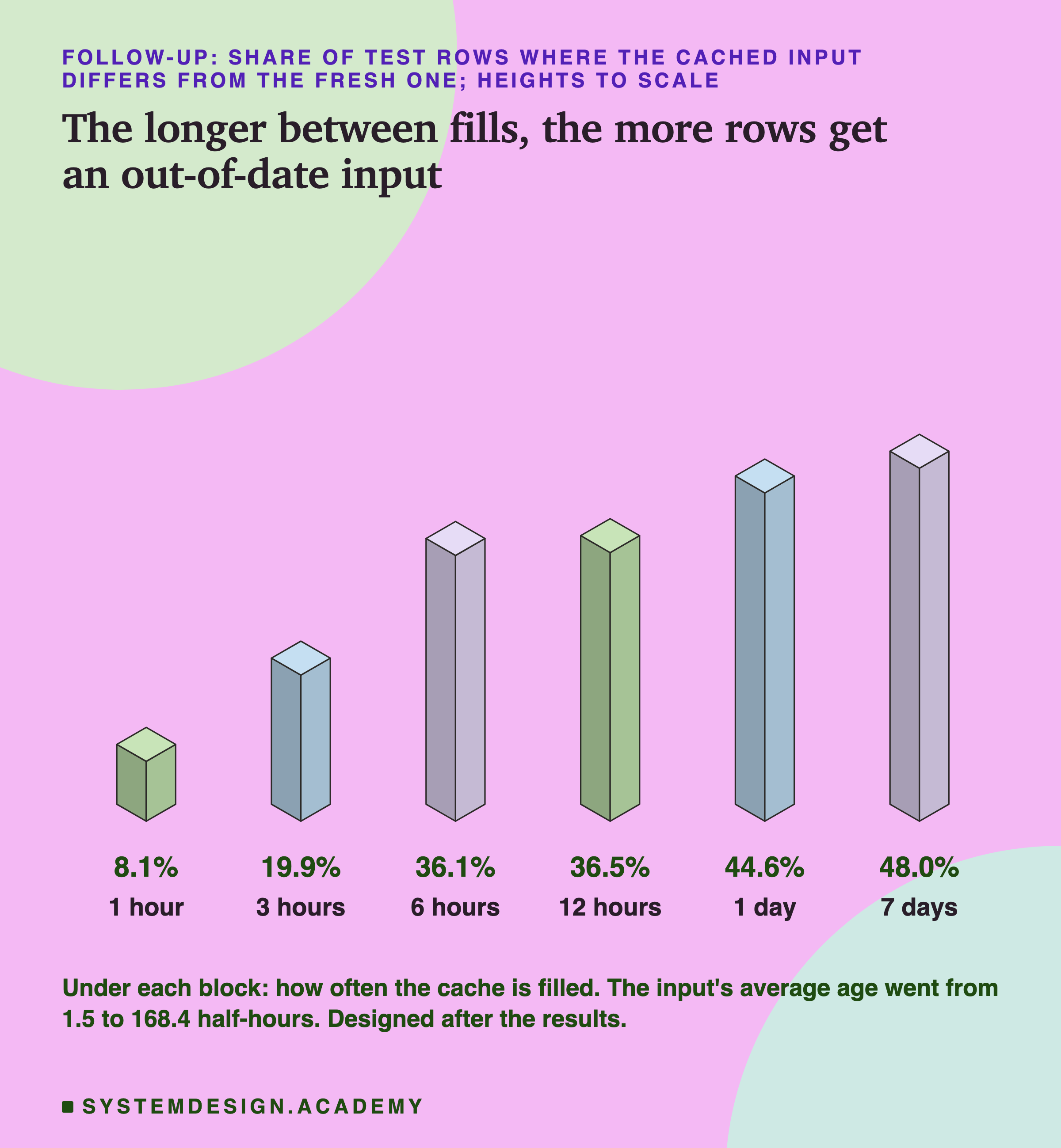
The share of rows with an out-of-date input rose with the interval: 8.1% for one hour, 19.9% for three, 36.1% for six, 36.5% for twelve, 44.6% for a day and 48.0% for a week. The last is close to what two unrelated labels would give, so a week-old lag carries almost no information about now.

The practical reading: for an input that changes every half-hour and that the model relies on, there is no cache interval that is free. Even one hour cost almost a point here. For an input that changes slowly, such as a customer's country, a day-old cache might cost nothing. The number that decides it is how often the cached value would differ from a fresh one, and you can measure that before you choose the interval.

The same follow-up asked which inputs carried the stale scaler's damage. It used the training scaler for every input except the named ones, which got the old scaler's average and spread.

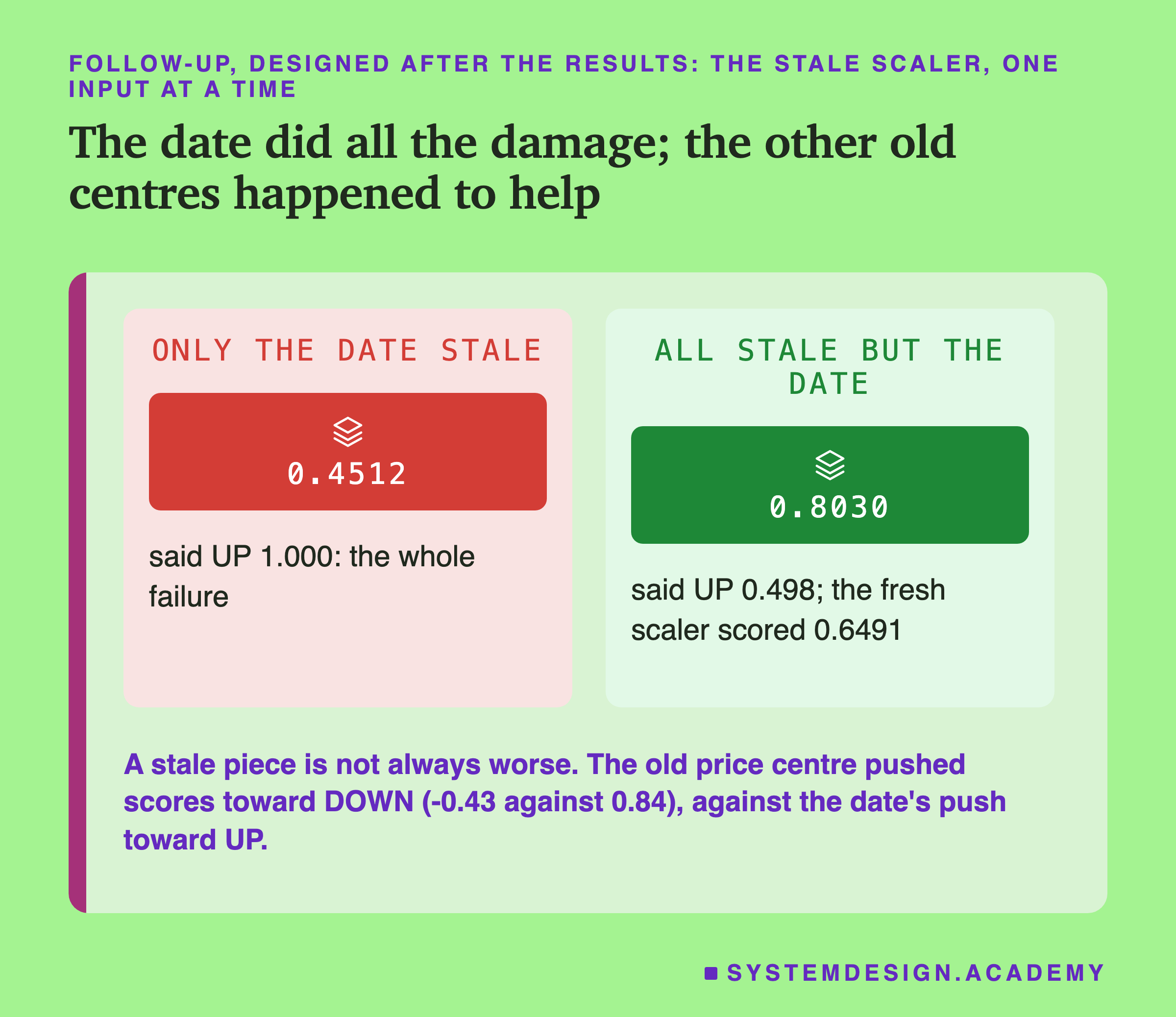
With only the date stale, the model scored 0.4512 and said UP on every row: the whole failure, from one input. With every input stale except the date, it scored 0.8030. That is 15.39 points better than the logistic model with the right scaler, and I did not expect it.

Here is what I measured, after the results. With the right scaler, the date pushed the average score toward UP by 1.19 and the price by 0.84, and the model said UP on 75.7% of rows when only 45.1% were UP. The old scaler's average price was higher than the training average, so with it the price pushed the average score toward DOWN by 0.43 instead. One possible reason for the jump, and it is my reading rather than a test: that old price centre happened to cancel most of the date's drift toward UP, so the mix of answers came out close to reality.

I include this because it teaches something uncomfortable. A stale piece is not always worse, and a pipeline that mixes old and new pieces can score better by accident. That does not make the old piece right. It makes the model's behaviour depend on a coincidence nobody chose, which can reverse with the next month of data. The fix is still to load the scaler that belongs to the model.

The checks on the previous slide look at inputs and outputs. Two cheaper checks look at the pipeline itself, and neither needs the right answers. I measured both after the results.

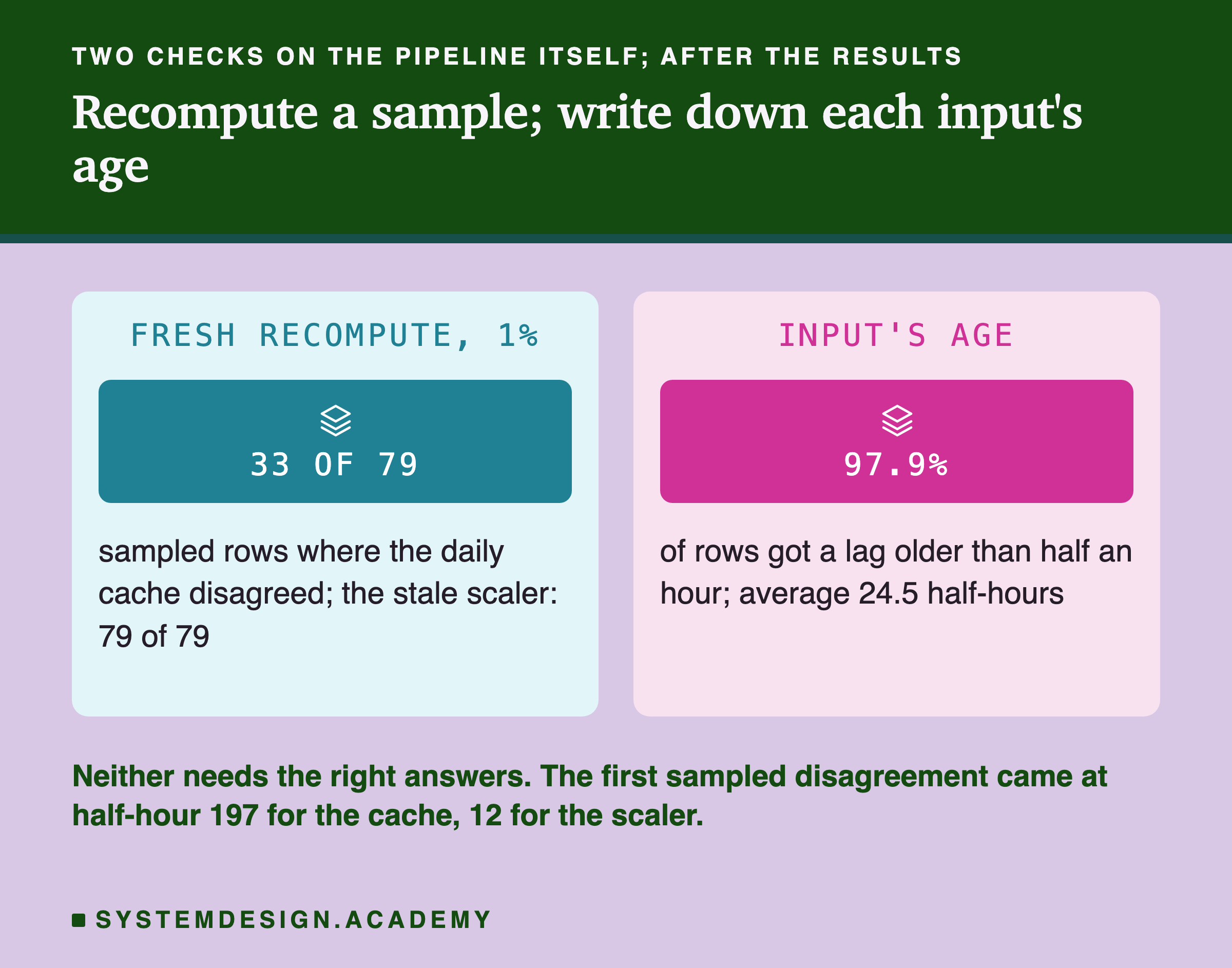
Recompute a small sample fresh. Pick 1% of served rows at random, compute their inputs again from scratch, the slow way, and compare with what the pipeline served. Here each of the 9,063 test rows had a 1% chance of being picked, with seed 0, which gave 79 rows. The daily-cached lag disagreed with a fresh computation on 33 of them, the first at half-hour 197, about four days in. The stale scaler disagreed on all 79, from the first sampled row. Any disagreement at all is worth an alarm, because a fresh recompute and a correct cache should agree on every row.

Write down each input's age. If the pipeline stores, next to every input it serves, the time the value was computed, then staleness is a number you can read. A fresh lag is always one half-hour old. The daily-cached lag was older than that on 97.9% of rows, on average 24.5 half-hours old and at worst 48. A rule such as "refuse a lag older than one half-hour" would have fired at once. The same idea works for artifacts: store, with the saved scaler, which rows it was fitted on. Here the scaler said 9 August 1996, and the model it served had trained up to 1 June 1998.

Here is what the lab points to, in the order a pipeline meets it.

Record when every input and file was computed. Store the time next to each cached value, and store with each artifact the rows or dates it was fitted on and the version of the model it belongs to. That turns "is this stale?" from a guess into a lookup.

Give every cache an expiry. Decide how old a value may be before the pipeline must compute it again, and make the pipeline refuse older values instead of serving them. Choose the expiry by measuring how often an old value differs from a fresh one: here a cache filled every hour, whose values were on average 1.5 half-hours old, already differed on 8.1% of rows.

Load artifacts by the model's version, not by a file path. The stale scaler here is what happens when a pipeline loads "the scaler" from a fixed place and a retrain replaces the model but not the file. If the model and its scaler are saved together, or the scaler is part of the saved model, they cannot drift apart. In scikit-learn, a Pipeline that holds both does exactly that.

Run input checks on what the model receives. Checks on raw inputs could not see the stale scaler at all. A range check on the standardised inputs, with a small margin, saw it on every day through the date. Add a stuck check for inputs that should move within a batch: it caught the daily cache on every day.

Watch the output mix over a long enough window. A single day's share of UP answers was inside the normal range even for a model that said UP on every row. Over a week, one answer on every row happened in none of 107 training weeks.

Recompute a small sample fresh, and compare. It is the one check here that caught both stale pieces, from the first days, without any labels.

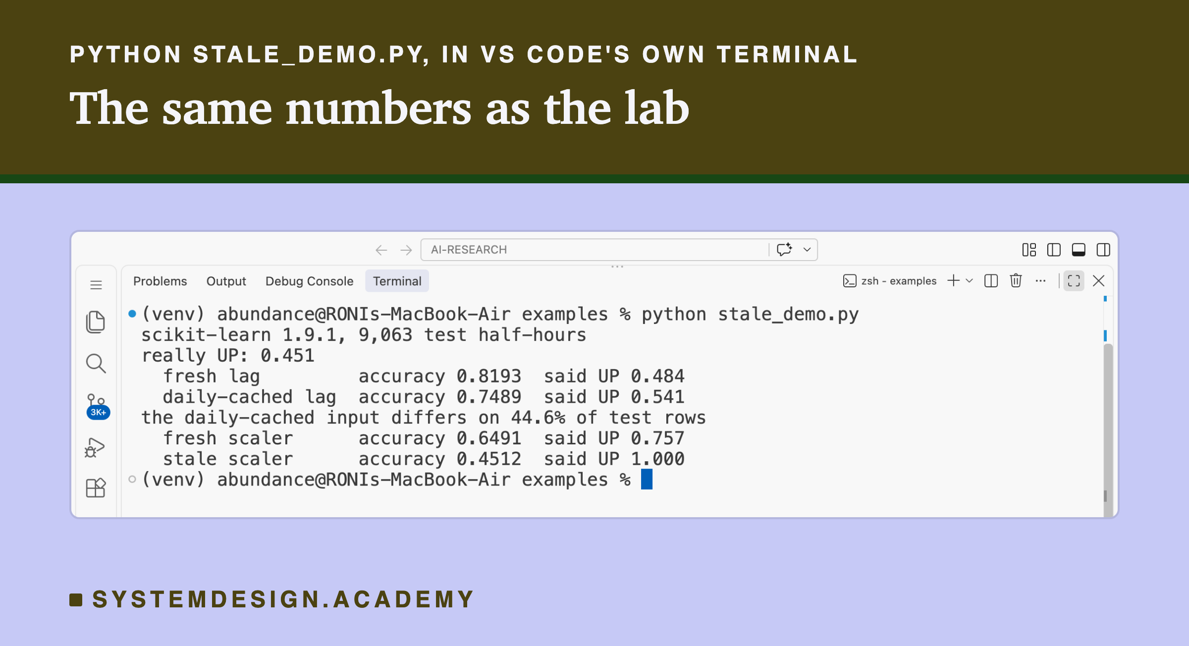
This script is the lab made small. It downloads the same data, trains the trees with the lag input and the logistic model with its scaler, and serves each one twice: fresh, and with a stale piece. For the trees the stale piece is the daily cache; for the logistic model it is a scaler fitted on the first 10% of the rows. It prints the accuracy and the share of answers that were UP for each, and how often the cached input differs from the fresh one. It does not need a GPU.

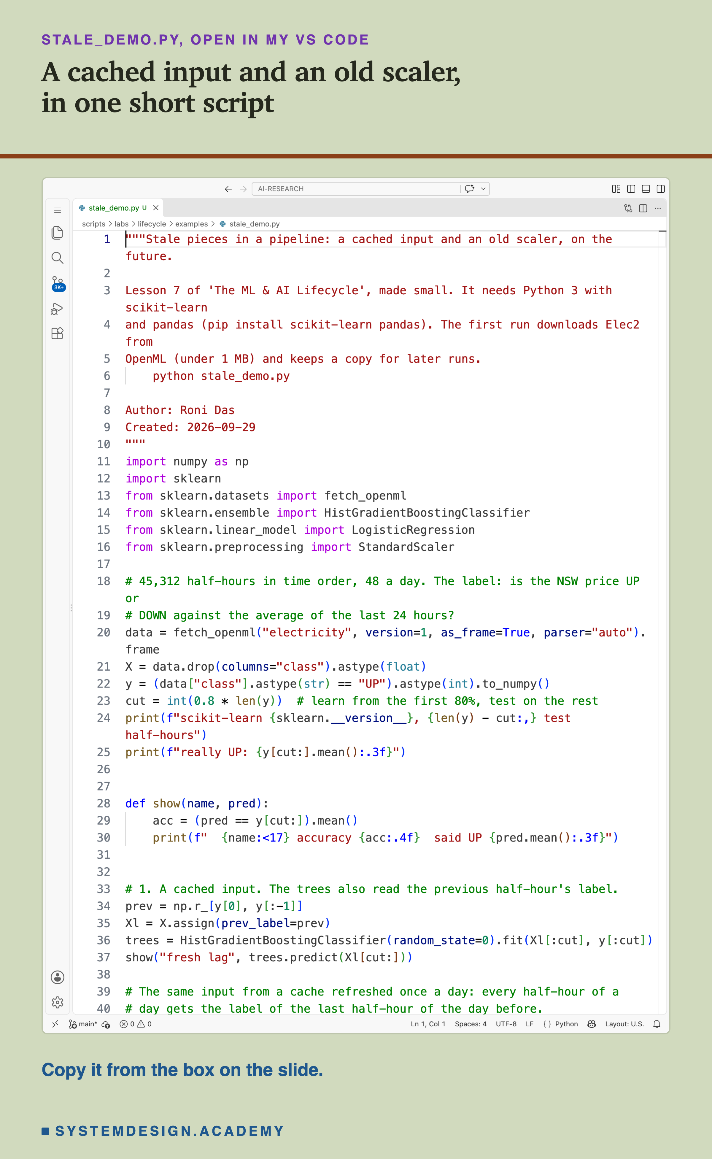
Before you run this lab. You need Python 3 and two libraries: pip install scikit-learn pandas. scikit-learn holds the models, the scaler and the download, and brings NumPy with it; pandas holds the table. The first run downloads Elec2 from OpenML (under 1 MB compressed), so it needs an internet connection once; scikit-learn keeps a copy in a folder in your home directory (scikit_learn_data) for later runs. It trains two small models, so it is quick; I did not time it. I ran it with scikit-learn 1.9.1 on a Mac. scikit-learn runs the same way on Windows and Linux, but I have not checked the numbers there, and another version of scikit-learn may give different decimals, which is why the first line printed is the version.

"""Stale pieces in a pipeline: a cached input and an old scaler, on the future.

Lesson 7 of 'The ML & AI Lifecycle', made small. It needs Python 3 with scikit-learn
and pandas (pip install scikit-learn pandas). The first run downloads Elec2 from
OpenML (under 1 MB) and keeps a copy for later runs.
    python stale_demo.py

Author: Roni Das
Created: 2026-09-29
"""
import numpy as np
import sklearn
from sklearn.datasets import fetch_openml
from sklearn.ensemble import HistGradientBoostingClassifier
from sklearn.linear_model import LogisticRegression
from sklearn.preprocessing import StandardScaler

# 45,312 half-hours in time order, 48 a day. The label: is the NSW price UP or
# DOWN against the average of the last 24 hours?
data = fetch_openml("electricity", version=1, as_frame=True, parser="auto").frame
X = data.drop(columns="class").astype(float)
y = (data["class"].astype(str) == "UP").astype(int).to_numpy()
cut = int(0.8 * len(y))  # learn from the first 80%, test on the rest
print(f"scikit-learn {sklearn.__version__}, {len(y) - cut:,} test half-hours")
print(f"really UP: {y[cut:].mean():.3f}")


def show(name, pred):
    acc = (pred == y[cut:]).mean()
    print(f"  {name:<17} accuracy {acc:.4f}  said UP {pred.mean():.3f}")


# 1. A cached input. The trees also read the previous half-hour's label.
prev = np.r_[y[0], y[:-1]]
Xl = X.assign(prev_label=prev)
trees = HistGradientBoostingClassifier(random_state=0).fit(Xl[:cut], y[:cut])
show("fresh lag", trees.predict(Xl[cut:]))

# The same input from a cache refreshed once a day: every half-hour of a
# day gets the label of the last half-hour of the day before.
day_start = (np.arange(len(y)) // 48) * 48
cached = prev[day_start]
show("daily-cached lag", trees.predict(Xl.assign(prev_label=cached)[cut:]))
differs = (cached[cut:] != prev[cut:]).mean()
print(f"the daily-cached input differs on {100 * differs:.1f}% of test rows")

# 2. A stale scaler. Logistic regression reads inputs rescaled to an average
# of 0 and a spread of 1, by a scaler fitted on the training rows.
scaler = StandardScaler().fit(X[:cut])
logistic = LogisticRegression(max_iter=1000)
logistic.fit(scaler.transform(X[:cut]), y[:cut])
show("fresh scaler", logistic.predict(scaler.transform(X[cut:])))

# The same model, served with an old scaler left in the pipeline: one that
# was fitted on the first 10% of the rows only.
old = StandardScaler().fit(X[: int(0.1 * len(y))])
show("stale scaler", logistic.predict(old.transform(X[cut:])))

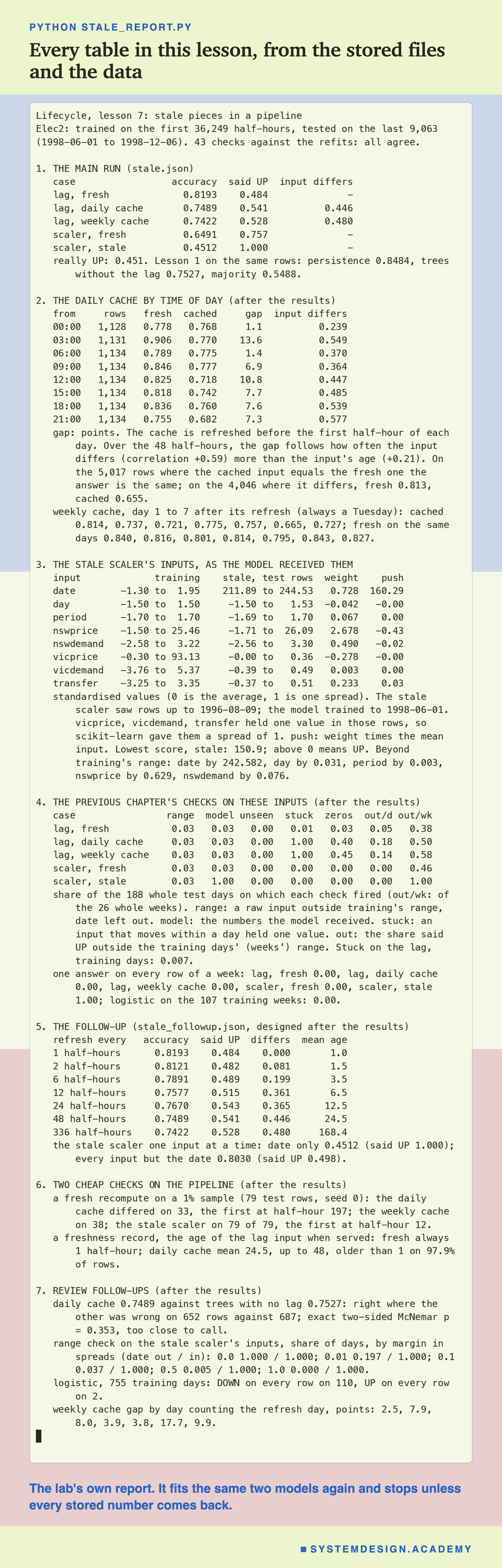
The report lives in scripts/labs/lifecycle/stale_report.py. It reads the lab's stored files, results/stale.json and results/stale_followup.json, lesson 1's results/baseline.json, and the Elec2 data from scikit-learn's local copy. The lab stored accuracies and shares, not each answer, so the report trains the lab's two models again with the same data, split and settings, rebuilds the five cases exactly as the lab did, and stops unless every stored accuracy, share and scaler average comes back exactly. It makes 43 checks in all, and they all agree. It changes nothing in the lab's files.

Its json mode writes every number to results/sa-report.json, which the figures read. The demo mode checks the student script's stored run, and the box mode writes the playground below and checks that it gives the lab's numbers.

This box has no model in it. It holds, for every one of the 9,063 test rows, the real label, the fresh and the daily-cached lag input, and the answers of all five cases, as two hexadecimal digits per row (counting in sixteens, with the digits 0 to 9 and a to f). The report checked that every accuracy, share, time-of-day block, stuck share and weekly mix it gives matches the lab's files. It runs in your browser.

As it is, the box prints the five cases with their accuracy and share of UP answers, how often the cached input differs, and the stuck check on the fresh and the cached lag: 0.005 of whole days against 1.0.

Then look at time of day with by_time_of_day('lag_daily_cache') and compare it with by_time_of_day('lag_fresh'). Try hours=1 for a finer view. Look at the output mix week by week with said_up_by_week('lag_daily_cache') next to said_up_by_week('lag_fresh'), and then said_up_by_week('scaler_stale'). Ask yourself which of them you would have noticed on a dashboard.

Loading. fetch_openml("electricity", version=1) downloads Elec2 once and reads the local copy after that. The label column holds the words UP and DOWN, turned into 1 and 0. cut is 36,249: the models learn from the rows before it and are tested on the 9,063 after it.

show. Prints one case: the accuracy against the real labels of the test rows, and the share of answers that were UP.

The fresh lag. prev shifts the labels down by one row, so each row holds the label of the half-hour before. X.assign(prev_label=prev) adds it as a ninth input, and the trees, with seed 0, learn from it. This is lesson 1's trees plus lag.

The daily cache. day_start gives each row the index of the first row of its day, because every day in Elec2 has exactly 48 rows. prev[day_start] then gives every row of a day the lag of the day's first half-hour, which is the label of the last half-hour of the day before. The trained trees are not touched; only their input changes.

The scalers. StandardScaler().fit(X[:cut]) learns each input's average and spread from the training rows, and the logistic model learns from the standardised rows. old is a second scaler fitted on the first 10% of rows only. The last line serves the same logistic model through the old scaler.

In the lab file, stale_lab.py does the same for the five cases, adds the weekly cache, and stores the numbers and both scalers' averages in . Its mode adds the other cache intervals and the scaler one input at a time.

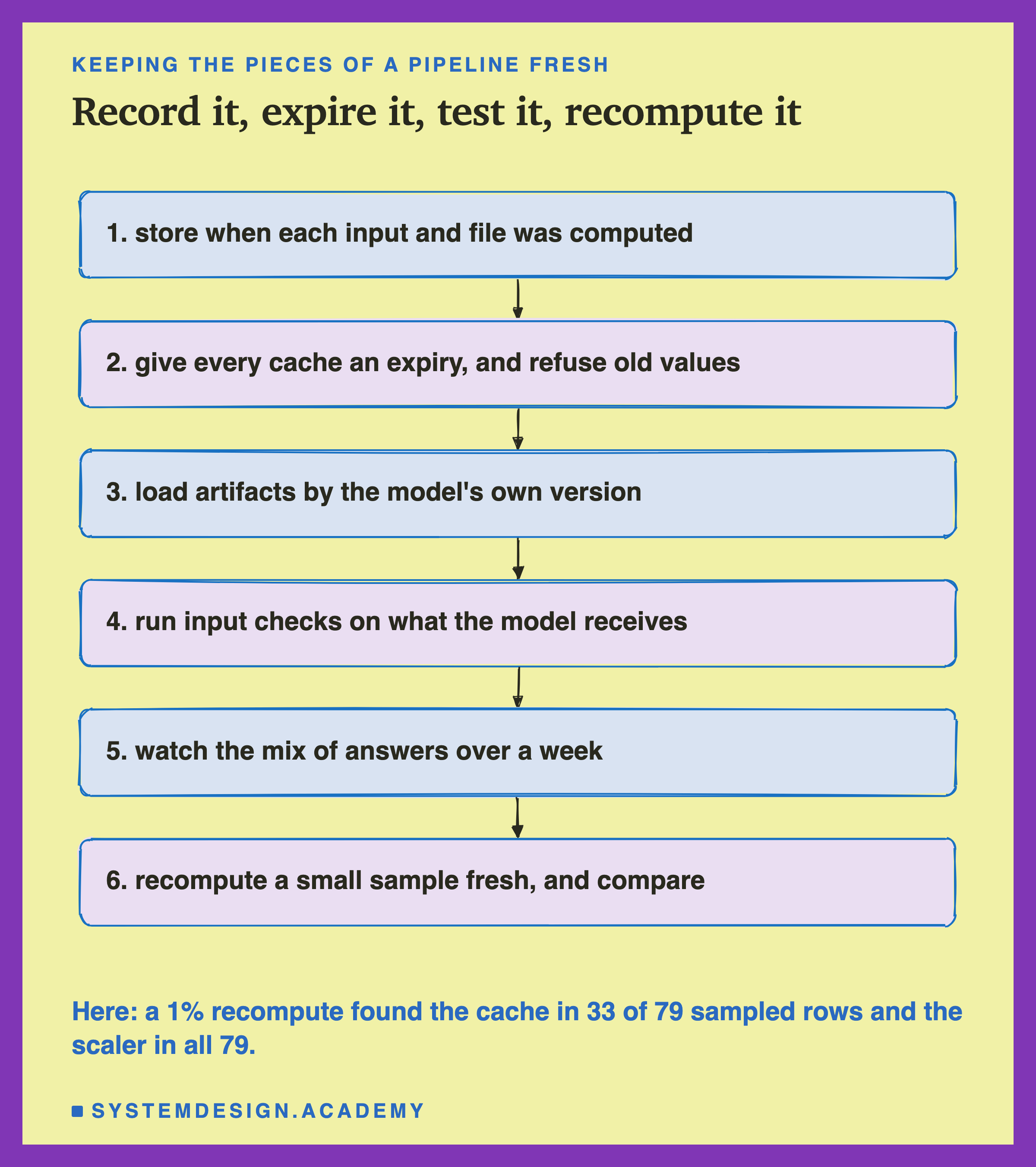
Store when each piece was computed. For every cached input, keep the time it was computed next to the value. For every artifact, keep the data it was fitted on, the date, and the model version it belongs to. This is often called lineage, and the next lesson planned for this chapter measures what it buys.

Give every cache an expiry. Before choosing it, compute, on past data, how often a value of each age differs from a fresh one. Choose the longest age whose disagreement you can accept, write it into the pipeline's configuration, and make the pipeline recompute or refuse any value older than that.

Keep the model and its artifacts together. Save the scaler inside the same object as the model, or give both the same version and load them by it. Never let a retrain replace one without the other.

Check what the model receives. Run range checks after every transformation, on the numbers that reach the model, and a stuck check on inputs that should move within a batch.

Watch the output mix over a long window. A day can be unusual for good reasons. A week of one answer should not happen.

Recompute a sample. Every day, recompute 1% of served inputs from scratch, compare, and alarm on any disagreement.

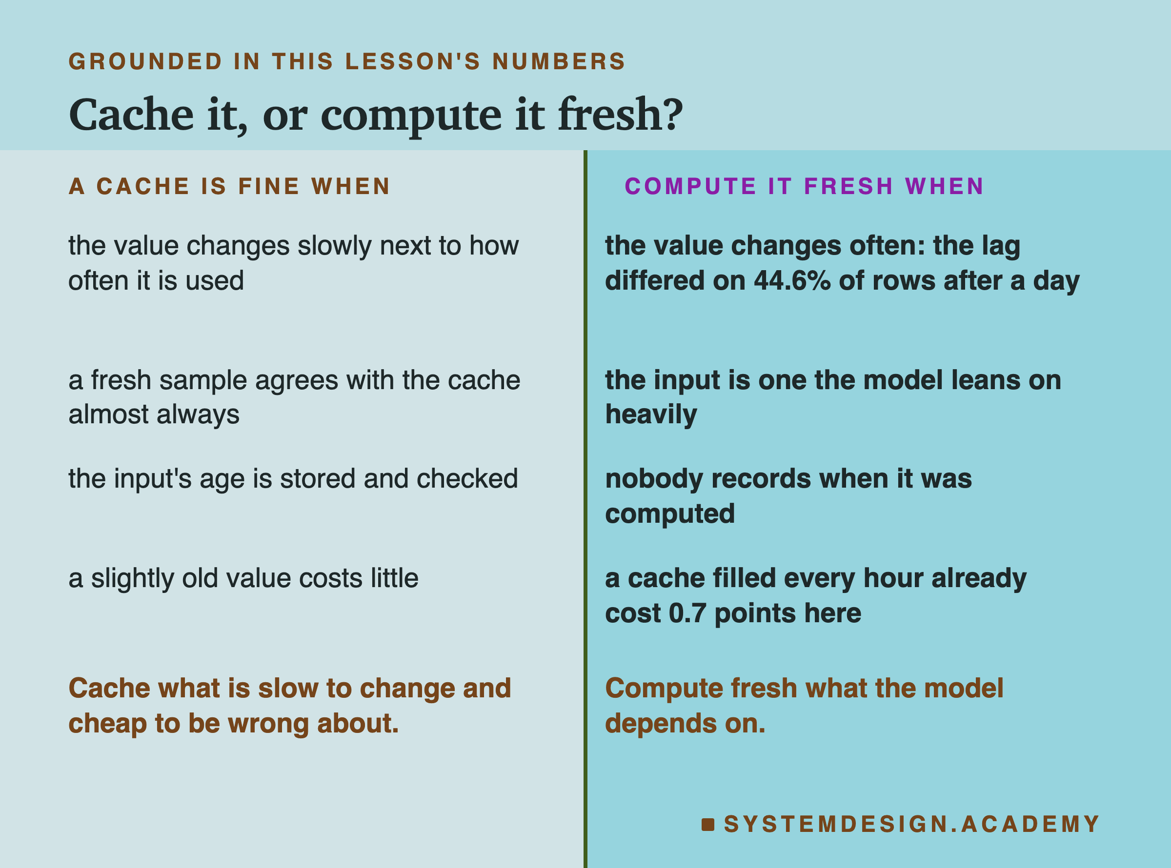
Use a cache when the value changes slowly compared with how often it is read. A customer's country, a product's category or last month's average barely change within a day. Caching them for a day costs little and saves a lot of work.

Use a cache when a fresh sample agrees with it almost always. Measure it: if a fresh recompute and the cache disagree on a tiny share of rows, the cache is doing its job.

Use a cache only when its age is stored and checked. A cache with a recorded age and an expiry is a decision. A cache without them is a guess that nobody will revisit.

Do not cache an input that changes as fast as the model's answers. Here the lag changed within hours, and even a one-hour cache cost 0.72 points.

Do not cache an input the model leans on heavily without measuring the cost. Here a day-old lag left the trees about the same as trees that never had the lag, 0.7489 against 0.7527, and all 7.04 points the lag had added were gone.

Do not reuse a fitted artifact across retrains. A scaler, an encoder or a vocabulary fitted once belongs to the model it was fitted with. Here an old scaler turned a model that scored 0.6491 into one that said UP on every row.

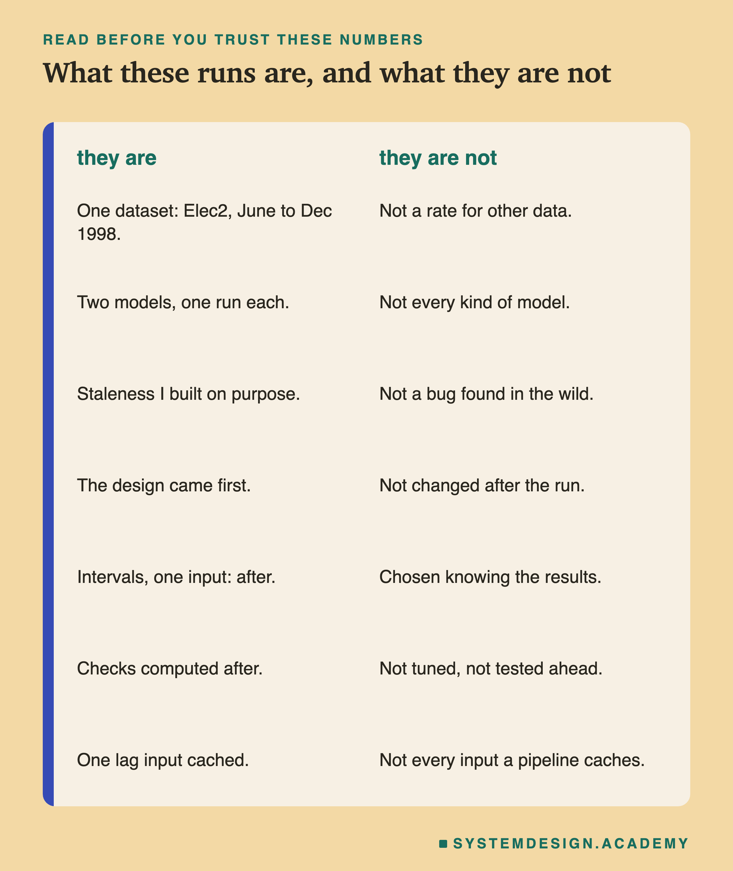
One dataset, two models, one run each. Everything here is one electricity market in the second half of 1998, lesson 1's trees plus lag and its logistic model. With other data, other inputs and other models, the costs would move. No significance test was declared, so I do not call any gap significant.

Staleness I built on purpose. The caches and the old scaler are faults I put into the pipeline to measure them. They are the kind of fault that happens in real systems, but they are not a bug I found in someone's system, and a real stale piece might be stale in a messier way.

One input cached, one scaler stale. Real pipelines cache many inputs at many intervals. What a stale input costs depends on how much the model relies on it and how fast it changes; the lag here is an extreme case on both counts, which makes it a clear demonstration and a poor estimate for other inputs.

The follow-up came after. The cache intervals and the scaler one input at a time were designed after I saw the main results and written down before they ran.

The checks came after. The previous chapter's checks were computed on these inputs after the results, with rules I wrote knowing what I was looking for. They show which kind of check can see which kind of staleness; they are not a fair trial of the checks. The reasons for the time-of-day pattern and for the 0.8030 are my reading, labelled as such.

Take the pipeline of a model your team runs, and list every stored piece in it: every cache, every saved file that a step loads. For each one, ask the five questions on the card. If the answer to "when?" is "we do not know", start there. Adding a timestamp to a cached value is a small change, and it makes every later question answerable.

Then run a small version of this lab on your own pipeline. Take a day of served rows, recompute their inputs from scratch the slow way, and count how many disagree with what was served. If the answer is zero, you have learned your caches are healthy. If it is not zero, you have found a stale piece before it found you.

The chapter plan's next lesson is lineage and rollback: rebuilding last month's model exactly, and what breaks when you cannot.