Imagine a small bakery chain with twelve shops. Every evening each shop sends the head office one sheet of paper: what it sold that day, hour by hour. A clerk at the head office copies every sheet into one big book. On Sunday the owner reads the book and decides how much bread each shop should bake next week.

Now four small things happen, and none of them makes a sound.

A courier hands over a sheet, but the clerk's receipt blows off the desk, so the next morning the courier comes back with the same sheet. The clerk copies it in again. That shop's Tuesday now counts twice.

One shop's sheet arrives on Monday, after the clerk has already closed last week's page. That day is simply missing from the book.

Another sheet arrives cut into strips and mixed up, because the shop printed it in pieces. The clerk copies the strips in the order they came out of the envelope. Next to each hour the clerk also writes "busier or quieter than the hour before", and now that note compares each hour with a random other hour.

A fourth shop starts using a new form, where the box that used to say "loaves" now says "bread, units". The clerk looks for "loaves", does not find it, and writes nothing.

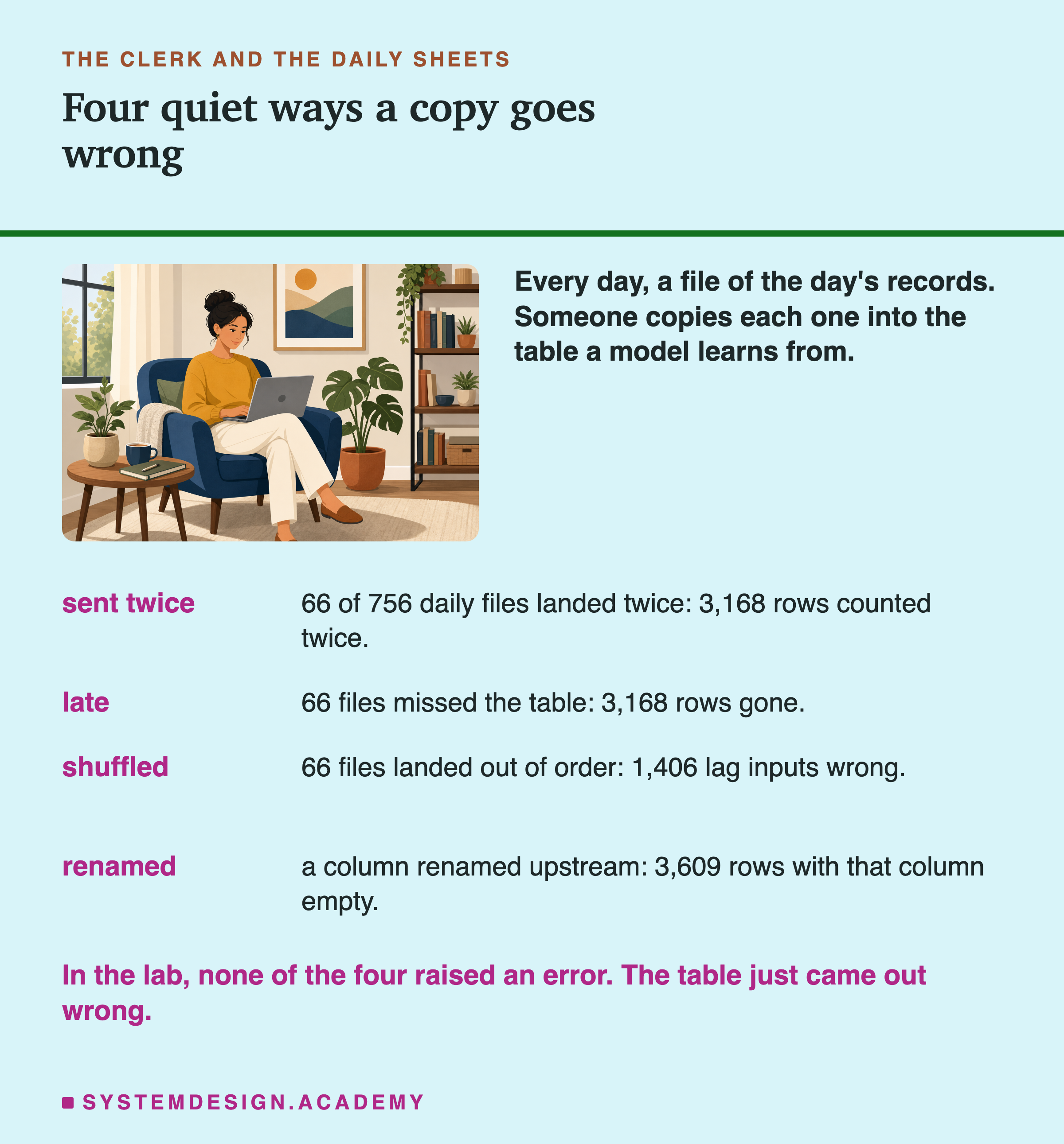
Every one of these leaves the book looking normal: neat handwriting, the right pages, numbers in every column but one. The owner will bake too much or too little, and nobody will know why. This lesson is about that clerk's job in a data platform, where the sheets are files of records and the book is the table a model learns from. The four numbers in the picture come from the lab later in this lesson. There I made each of these mistakes happen on purpose, and measured what it did.

The previous lesson compared two ways to move data: in batches on a schedule, and as a stream, one event at a time. This lesson looks at the step that comes first in both: copying data out of the systems that run a business and into the place where models learn. That step is called ingestion.

In most companies, the data a model needs lives in systems built for something else. Think of the shop's order database, the app that records every tap, or a partner that sends a file every night. Ingestion is the work of copying that data out, safely and completely, into storage the data team controls. Everything a model learns later is built from that copy, so a mistake at this step reaches every number built from it and every model trained on it.

The lesson has two halves. The first half explains the ideas: where data comes from, who starts each transfer, and the three common ways to copy it. It also covers the problems that make ingestion hard: copies, bursts, late data and changing columns. The first version of this lesson stopped there. For this version I checked every claim in it against the tools' own documentation, and fixed or cut the ones that did not hold. The list of claims, sources and verdicts is in the lab folder, in scripts/labs/dataeng/results/ip-factcheck.json.

The second half measures. I took real data, sent it through a small copying pipeline one file a day, and broke the pipeline in four quiet ways, the clerk's four mistakes. Then I asked three questions. What did each fault do to the table? What did it do to a model trained on that table? Which simple check would have noticed?

The answer surprised me. The model's accuracy was a poor alarm. It went up for some faults and down for others. Retraining the same model on the same clean table, with only the random seed changed, moved it more than most faults did. Six cheap checks on the table itself, which need no right answers and no model, caught each of the four faults in every run. I wrote each check knowing which fault it was for, so that part was expected; the limits slide says what they would miss.

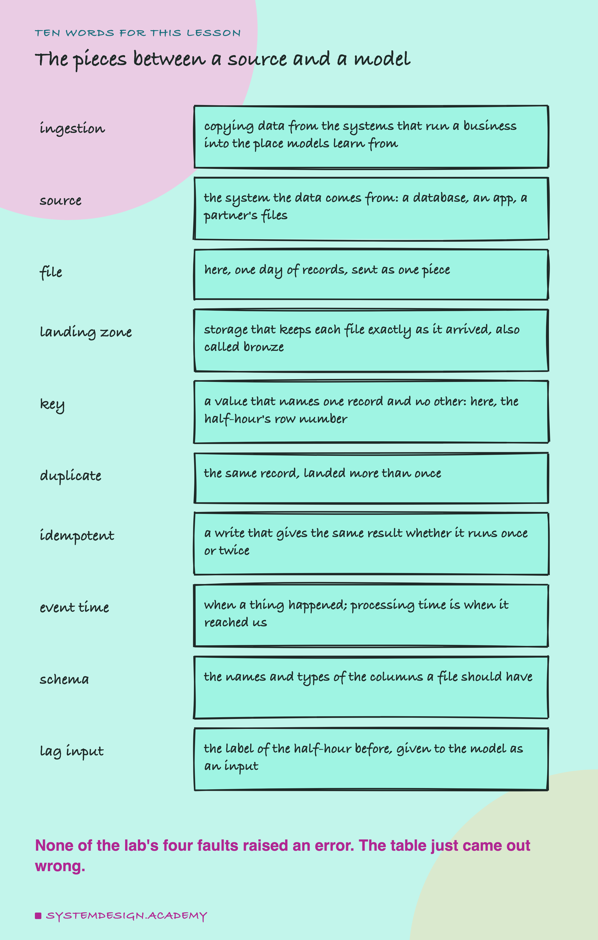
Ingestion is copying data from the systems that run a business into the place models learn from. The system it comes from is the source. In this lesson's lab the source sends one file a day: that day's records, as one piece. The first place a file lands is the landing zone: storage that keeps each file exactly as it arrived. Many teams call it the bronze layer.

A key is a value that names one record and no other, like an order number. When the same record lands more than once, the extra one is a duplicate. A write is idempotent when doing it twice gives the same result as doing it once. Setting a box to 5 is idempotent; adding 5 to it is not.

Event time is when something happened; processing time is when it reached us. A schema is the list of column names and types a file should have.

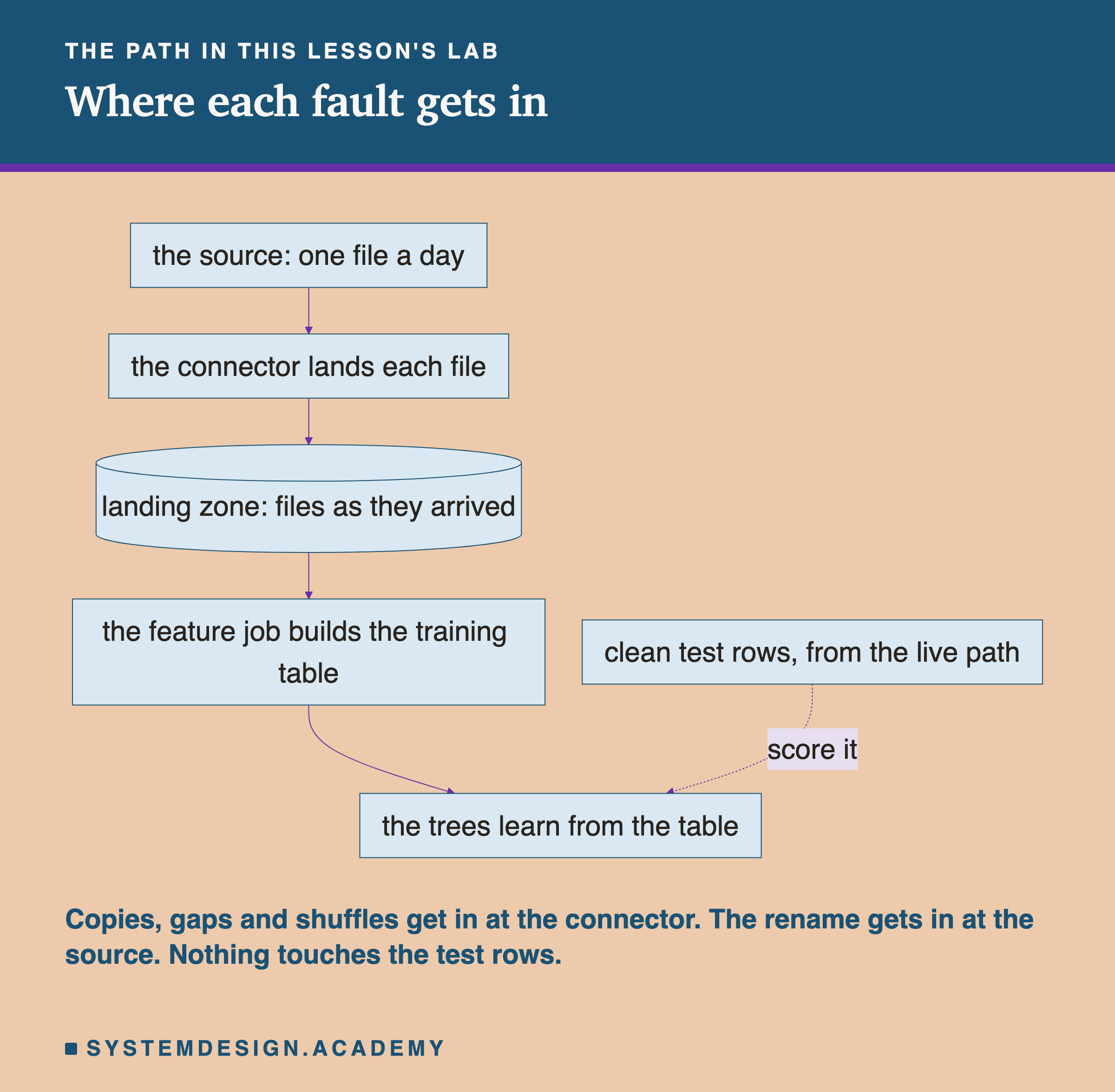
The lab's model predicts, for each half-hour, whether an electricity price went up or down. That right answer is the label. The model is also given the label of the half-hour before as one of its inputs, which I call the lag input. A feature is any input a model reads. Accuracy is the share of rows a model got right, and a point is one hundredth of accuracy. Here is the path those words describe, as the lab builds it.

Here is a story I made up to show the problem. I have not measured it, but each part of it is how these systems behave.

A data scientist builds a recommendation model. It needs three inputs: how many orders each user placed this week, their average basket size, and whether they opened the app today. All three live in the production Postgres database that runs the shop. So the first version of the model simply queries that database each time it makes a prediction.

It works in the demo. Then it goes live, and checkout slows down. The model's big analytical queries compete with real customers for the same processors and the same disks. A long-running read also holds back Postgres's clean-up of old row versions, a job called VACUUM, so busy tables grow bloated.

One thing does not happen: in Postgres a plain read never blocks an ordinary write, an INSERT, UPDATE or DELETE. Its documentation says "reading never blocks writing and writing never blocks reading", because readers and writers see separate versions of each row. There is one exception worth knowing. Most forms of ALTER TABLE need the strongest lock, and a running read does block that. While the ALTER TABLE waits, the writes that arrive after it wait behind it. The database team bans the model from production anyway, and the project stalls.

So a model should not read the live product database, and it should not depend on a source it does not control. Instead, you copy the data you need into the platform, on your own schedule, in your own shape, without disturbing the systems that run the business. That copying is ingestion, and every later lesson in this chapter builds on it.

There is a second, quieter reason ingestion matters. It sets the freshness ceiling of every feature: the freshest a value can ever be. A feature computed from a source you copy once a night can never be fresher than a night old, however fast everything above it runs. That ceiling is set at the very first copy, and nothing downstream can raise it.

Every piece of data a platform ingests comes from one of four kinds of source, and each behaves differently.

• Databases (Postgres, MySQL, MongoDB). Structured, changing all day, and not for heavy reads in production.
• APIs (a payments provider, a weather service, a partner catalogue). An API is a door another company's system opens to programs: you ask, it answers, one page at a time, within a rate limit.
• Events (clicks, purchases, ride requests). Behaviour the app records as it happens, which often never lives in a table.
• Files (daily CSV or Parquet exports, vendor feeds, log dumps). Dropped into storage by systems you do not control. The lab's source is this kind.

Whatever the source, the first stop is the same: the landing zone. This is cheap object storage, usually Amazon S3 or something like it, where data lands exactly as it arrived, untouched. Keep two times with every record: when it happened, and when it arrived.

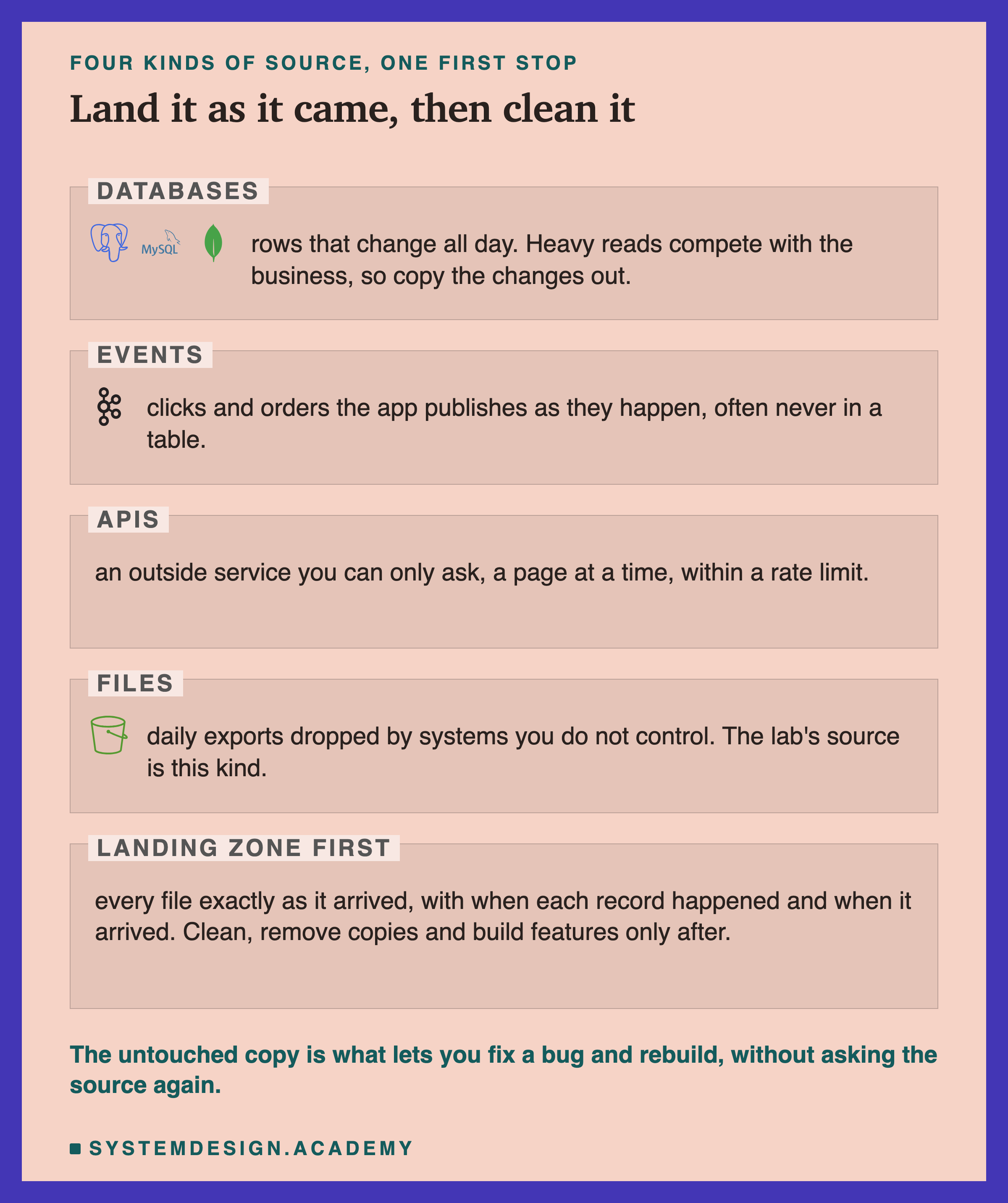
The rule that keeps this sane: land raw first, transform later. Storage is cheap per gigabyte, and that untouched copy is what makes recovery possible. If a cleaning job has a bug, you fix the job and rebuild from the landing zone. You do not go back to the source, because the source may have changed.

An order a customer edited yesterday looks different today, and a click a phone sent while offline is long gone from the app's memory. The landing zone is your one lasting record of what actually arrived. In the lab, every fix at the end works only because each landed file was still there to rebuild from.

Before you choose between batch, CDC and streaming, settle a simpler question: who starts the transfer? There are only two answers, and the choice decides who controls the timing and who carries the load.

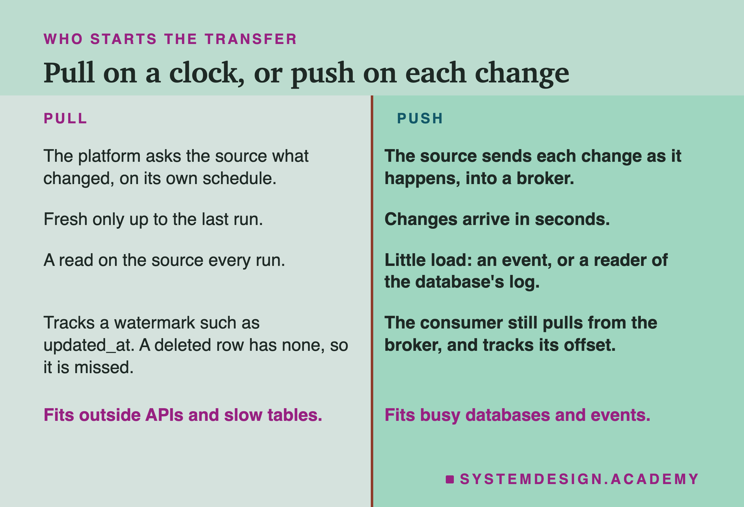
In a pull, the ingestion job reaches into the source and asks what changed, on a clock the platform owns. Batch jobs and API polling both work this way. The platform controls the timing, which is convenient. But features are only as fresh as the last run, and every run puts a read on the source that competes with real traffic.

To avoid reading everything each time, a pull keeps a watermark, usually a column like updated_at. Each run fetches only the rows changed after the highest value it saw last time. A deleted row has no updated_at left to find, so a watermark pull never sees deletes. Debezium's own article on this says polling "will not allow you to identify any records that have been deleted since the last poll".

In a push, the source sends each change as it happens, and the platform only has to receive it. Event streaming and change data capture both work this way. Both usually deliver into a broker: a system such as Apache Kafka that stores messages until readers take them. Changes flow in seconds, and the source carries little extra load.

A few Kafka words first. A topic is a named stream of messages inside the broker. A producer is a program that writes messages to a topic, and a consumer is a program that reads them.

One detail is easy to miss. Even in a push design, the consumer pulls from the broker. Kafka's documentation says data is "pushed to the broker from the producer and pulled from the broker by the consumer". That lets a slow reader fall behind without breaking anything. The reader keeps its place with an : the position of the last message it finished. After a crash it carries on from there, instead of starting over or skipping ahead.

You rarely write ingestion by hand. You pick a connector, a ready-made program that knows how to read one kind of source, and the one you pick follows from the kind of source. Managed tools such as Airbyte and Fivetran each list hundreds of connectors. Debezium, the open-source tool for reading database change logs, covers about a dozen databases, in depth.

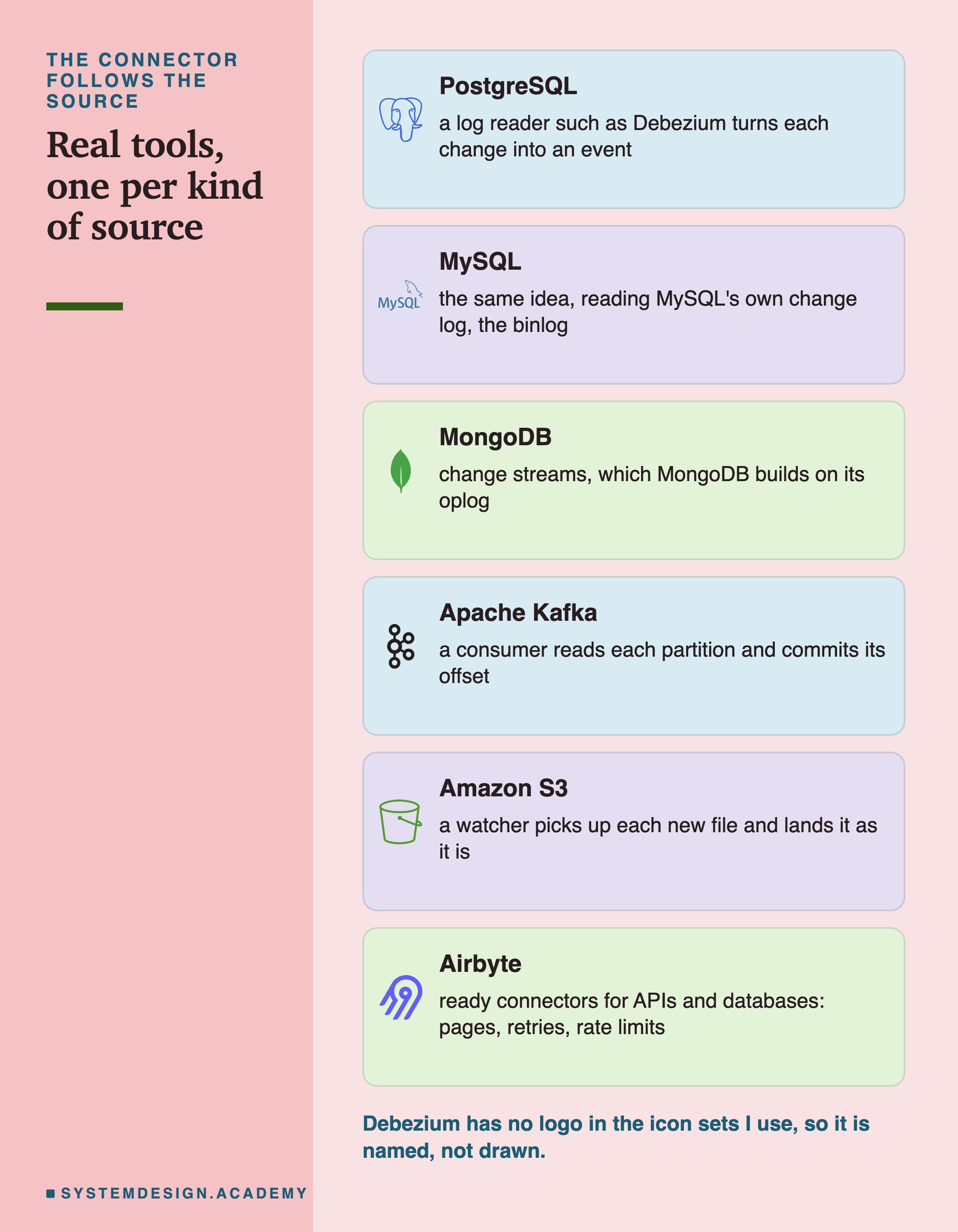
The reason to use a connector is not the easy part. Reading rows from a database or fetching a page from an API is simple. The value is in the edges. A good connector works through a large API result a page at a time. It waits and retries when an API answers 429, the HTTP code for "too many requests". It retries a dropped connection without losing its place, notices when the source's columns change, and saves its progress so a restart carries on cleanly.

Airbyte's documentation gives one example, for connectors built with its Connector Builder. When no error handling is set, they retry a request that got a 429 or a server error five times, waiting longer each time. Those are exactly the details a script written in an afternoon forgets, until the night it breaks. Write the connector yourself, and you volunteer to learn each of them again.

Once you know the source and who starts the transfer, you pick how to extract. There are three common ways, and the choice quietly sets the freshness ceiling from two slides back.

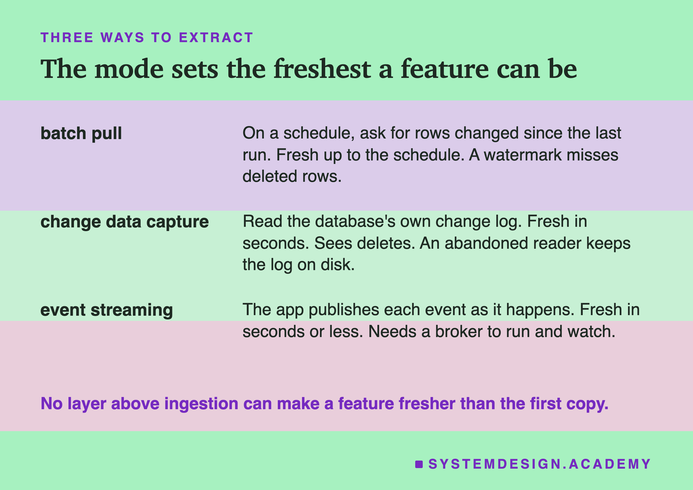
Batch pull is the simplest. On a schedule, you ask the source for everything changed since last time, usually by tracking a watermark like updated_at. Hourly, nightly, whatever the clock says. It is easy to reason about and cheap to run, but features are only as fresh as the schedule, and a watermark misses deleted rows.

Change data capture (CDC) reads the database's own change log and turns every insert, update and delete into an event. In Postgres that log is the write-ahead log, or WAL; in MySQL it is the binlog. For MongoDB, Debezium reads change streams, which MongoDB builds on its own log, the oplog. CDC reads the log instead of querying tables over and over. So it puts little load on the source, it sees deletes, and changes arrive close to real time.

Event streaming captures things as the application does them, publishing to a broker such as Kafka the moment a click or a purchase happens. It is the usual way to ingest behaviour that never touched a database; log files shipped to storage are another.

CDC feels like magic the first time you see it, so here it is slowly. The surprising part is how little the source has to do.

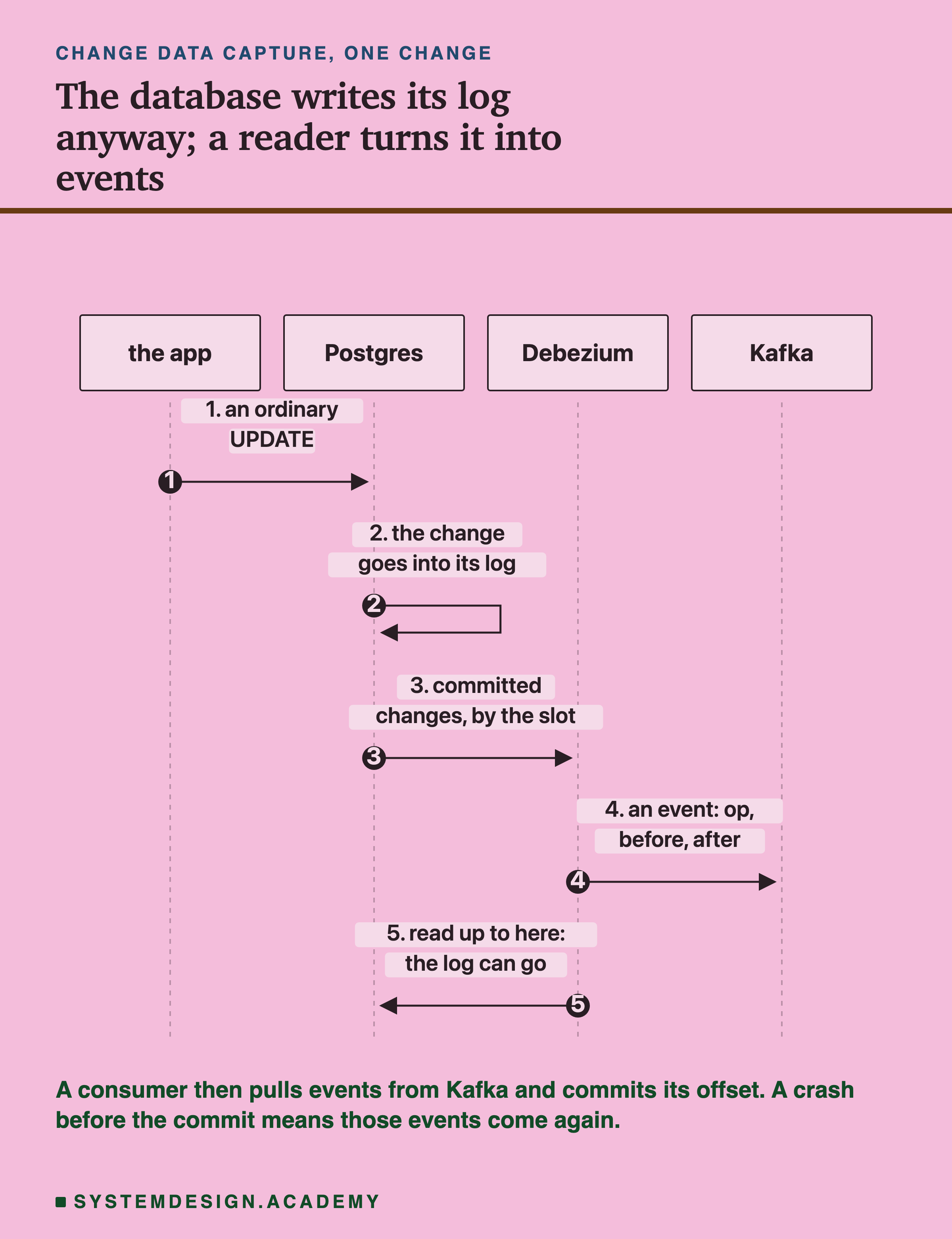
The application writes to Postgres exactly as it always has. It has no idea CDC exists. Postgres, for its own crash recovery, writes every change into its write-ahead log first, including changes from transactions that later roll back. A tool like Debezium holds a replication slot: a named bookmark in that log that Postgres keeps for one reader.

Through the slot, Postgres hands over each transaction once it commits. By default, its documentation says, changes are "only passed to the output plugin at commit (and discarded if the transaction aborts)". Since Postgres 14, a plug-in can also choose to receive a large transaction in pieces before it commits; that is an option, not the default. After a first snapshot, which does read each table once with an ordinary SELECT, Debezium reads only the log to find changes.

Each change becomes an event that says what happened (op: create, update or delete) and carries the row's values. after is the new row. before holds the old row in full only when the table's REPLICA IDENTITY setting is FULL. With the default setting, update and delete events carry old values for the primary key columns only. PostgreSQL's description of its replication messages adds that for an update, even the old key is sent only when the update changed it. That matters if a feature needs to know what a value used to be.

A note on sources. Debezium's documentation describes REPLICA IDENTITY the same way, but its worked example of an update shows the key in although the key did not change. The wording above follows PostgreSQL's own pages on ALTER TABLE and on the logical replication message formats. Check what your version sends before a feature relies on .

You rarely write CDC by hand. You configure a connector and let it run. Debezium is the open-source engine most teams reach for. Managed platforms like Fivetran and Airbyte wrap the same idea, if you would rather not run the plumbing yourself. Here is a trimmed Debezium connector config that captures changes from two Postgres tables and publishes them to Kafka.

{
  "name": "orders-cdc-connector",
  "config": {
    "connector.class": "io.debezium.connector.postgresql.PostgresConnector",
    "database.hostname": "orders-db.internal",
    "database.port": "5432",
    "database.user": "debezium",
    "database.dbname": "shop",

    "plugin.name": "pgoutput",
    "slot.name": "debezium_orders",
    "publication.autocreate.mode": "filtered",

    "table.include.list": "public.orders,public.order_items",
    "topic.prefix": "shop",

    "snapshot.mode": "initial",
    "tombstones.on.delete": "true",
    "decimal.handling.mode": "string"
  }
}

A few lines carry most of the weight. plugin.name chooses how Postgres turns its log into messages. Debezium's default is decoderbufs, a plug-in you must install on the server. pgoutput is built into Postgres 10 and later. The documentation of Amazon RDS, Azure Database for PostgreSQL and Google Cloud SQL names other plug-ins, such as wal2json, but not decoderbufs. So pgoutput is the one of Debezium's two choices that all three offer, and it is set here on purpose. slot.name is the replication slot that remembers how far Debezium has read, so a restart carries on cleanly.

snapshot.mode: initial matters on the first start, when the connector has no stored position. It reads every row of each table as it is at that moment, then switches to reading the log from that point. You get the current state plus every change after it, without a gap, but not the past edits of each row.

CDC and streaming solve freshness, but they bring a problem batch never had. A source can produce faster than the pipeline can write. During a sale or a dinner rush the buffer between them fills, and what happens next decides whether ingestion survives the burst.

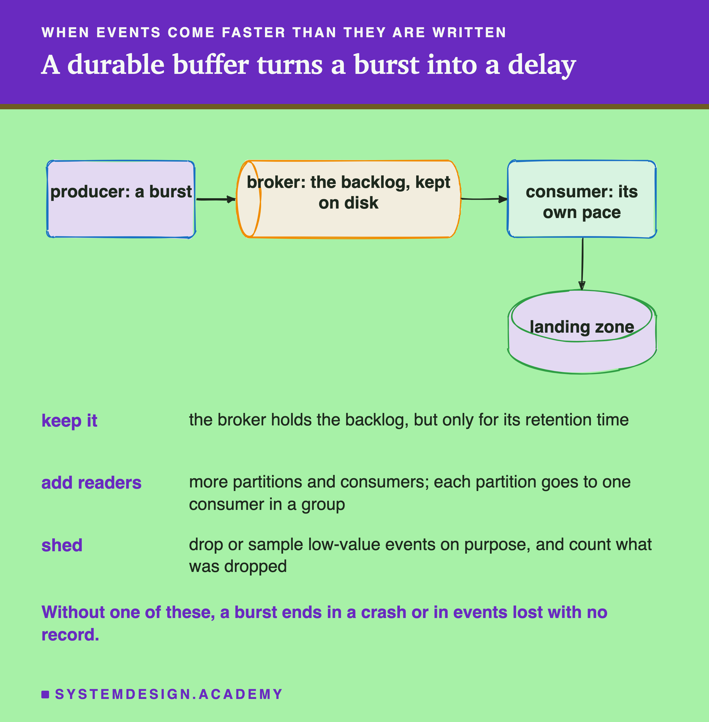
Backpressure is the signal that runs the other way, from the overwhelmed reader back toward the writer. When the buffer passes a high-water mark, the system does one of two things. It tells the writer to slow down, or it keeps the backlog in lasting storage and lets the reader catch up at its own pace. Either way the burst is absorbed instead of dropped. Without it, a spike ends in one of two ugly ways. The reader runs out of memory and crashes. Or events are thrown away with no record that they ever existed, which quietly skews every feature built from that window.

There are three levers, and mature platforms use all three.

Keep it. A broker such as Kafka holds the backlog on disk, so a slow reader only lags, but only for as long as the topic keeps data. Kafka's default retention is 168 hours, a week. A reader further behind than that has lost those events, and with the default setting it jumps ahead to the newest data without an error.

Add readers. A topic is split into partitions: separate, ordered pieces of its log that can be read in parallel. A consumer group is a set of consumers that share the reading of one topic. More partitions and more consumers raise throughput, with one limit: each partition goes to exactly one consumer in a group, so extra consumers get none.

Shed. Under extreme load, when freshness matters more than completeness, drop or sample low-value events on purpose. Count what you dropped, so the loss is on record. A durable buffer plus a slow-down signal turns a possible outage into a delay that drains on its own once the surge passes.

Any pipeline that retries can deliver a record more than once, and you cannot know in advance which records. Kafka's default is at-least-once. A producer retries after a timeout, sometimes when its first try already worked but the acknowledgement never came back. In current Kafka the producer is idempotent by default, so such a retry does not write a second copy. Its settings say "Idempotence is enabled by default if no conflicting configurations are set". When idempotence is off, or turned off by conflicting settings, retries "may write duplicates of the retried message".

Idempotence in the producer does not help further along the pipe. A connector that restarts, or a consumer that reads again after a crash, can still deliver a record twice. And a partner re-sends yesterday's file because their job failed halfway.

If your pipeline simply appends, the training table quietly counts some things twice. A feature like "orders this week" then reads high for exactly the users whose records were retried. The pipeline never errors, and the number looks believable. Here is what that looks like in the lab, where the connector sent a tenth of the daily files twice and the job appended both copies.

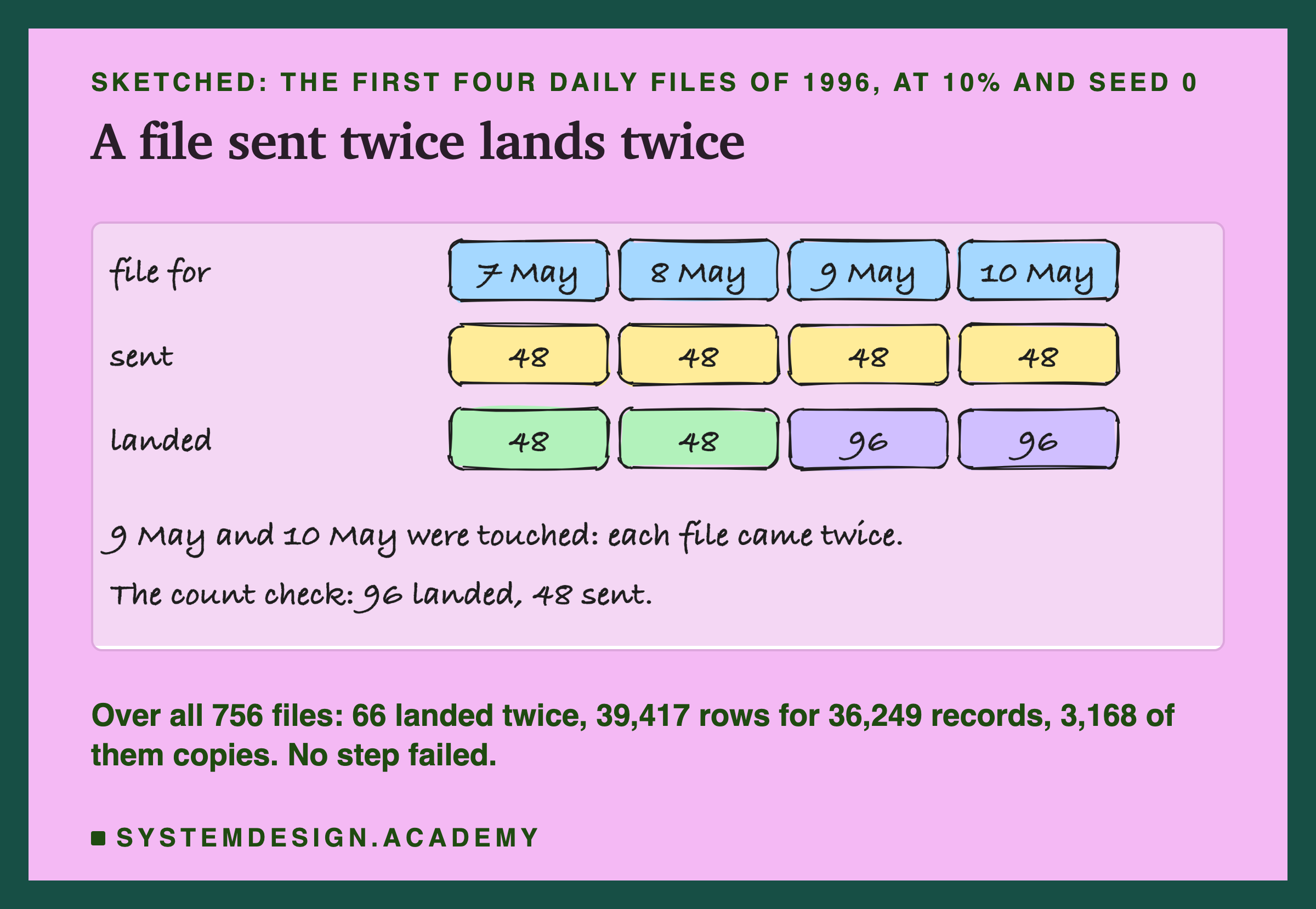
On the first four days of the data, two files came twice. The only visible sign was a count: 96 rows landed where the source had sent 48. Over the whole training window, 66 of the 756 files landed twice, so the table held 39,417 rows for 36,249 real records, and 3,168 of them were copies. No step failed. (The calendar here is rebuilt from row numbers, 48 half-hours a day from 7 May 1996, as the lifecycle chapter does.)

The defence is idempotency: make writing the same record twice give the same result as writing it once. You do that by giving every record a stable key, and by turning every write into a keyed upsert instead of a blind insert. An upsert updates the row if its key already exists, and inserts it if not.

The key is usually the source's primary key, like order_id. A version then decides which copy wins. Putting the version into the key would store every version as a separate row, which brings the duplicate problem back. The first time you see a key, you insert. When you see it again, you keep this copy only if its version is newer, because retries and out-of-order delivery mean a copy may be newer or older. Without that check, a late old copy would overwrite a newer value and quietly roll a row back in time.

Data does not always arrive when it happened. A phone is offline for two hours, then syncs. A partner batches its exports and sends them at midnight. A queue backs up during a traffic spike. This gap between event time, when the thing happened, and processing time, when you received it, is one of the trickiest problems in ingestion. The two terms come from Tyler Akidau's essays on stream processing, "Streaming 101" and "Streaming 102", published by O'Reilly.

Watch what goes wrong if you ignore it. An hourly job computes "features for the 10:00 window" at 11:00. It looks complete. Then at 12:30 an offline phone syncs its 10:00 click. If the window is built from what had arrived by 11:00, and never built again, the 10:00 features stay wrong for good.

If you train on that window, you teach the model from incomplete data. The error is invisible, because the window looked finished when you sealed it. The lab's late files are the same thing at the size of a day. There, 66 files had not arrived when the training table was built, so 3,168 rows were simply missing.

Two rules fix it. First, record both times with every record, and compute windows by event time, so a late record still counts in the window it belongs to. Many teams store the landing zone by arrival time, because it only ever grows at the end and device clocks can be wrong. They then group by event time in the next layer. Second, treat any feature computed near "now" as provisional, and run a backfill once late data has settled: re-run past windows to correct them.

In practice you also set a bound, a watermark in the streaming sense. This is a different use of the same word as the pull's watermark. Akidau defines it as "a notion of input completeness with respect to event times". In plain words: we will wait this long for stragglers, then finalise. You cannot keep every window open forever for a phone that may never reconnect.

A backfill is worth seeing as its own shape of run. The normal pipeline is incremental: each cycle takes one small, roughly constant slice of new data. A backfill is the opposite: one large sweep back over history. You run it to correct windows that late data changed, or to fill a new feature across all of its past.

It needs care an incremental run does not. A sweep over months of the landing zone can flood a broker, overload a database or run up a cloud bill if you run it at full speed. So limit its rate and run it off-peak. And lean on the idempotency from the last slide. Because the writes are keyed, a backfill that overlaps the live run lands in the same correct state, instead of fighting it.

Your ingestion runs perfectly for months. Then one morning it either crashes or, far worse, quietly starts writing empty values. A backend team shipped a change. They renamed a column, changed a type or dropped a field, and nobody told the data team, because nobody knew the data team depended on it. This is schema drift. Its cause is mostly organisational. The team that owns the source and the team that uses it are usually different, and the source team ships on its own schedule. Where the damage lands depends on a choice you made long before: where you enforce the shape of your data.

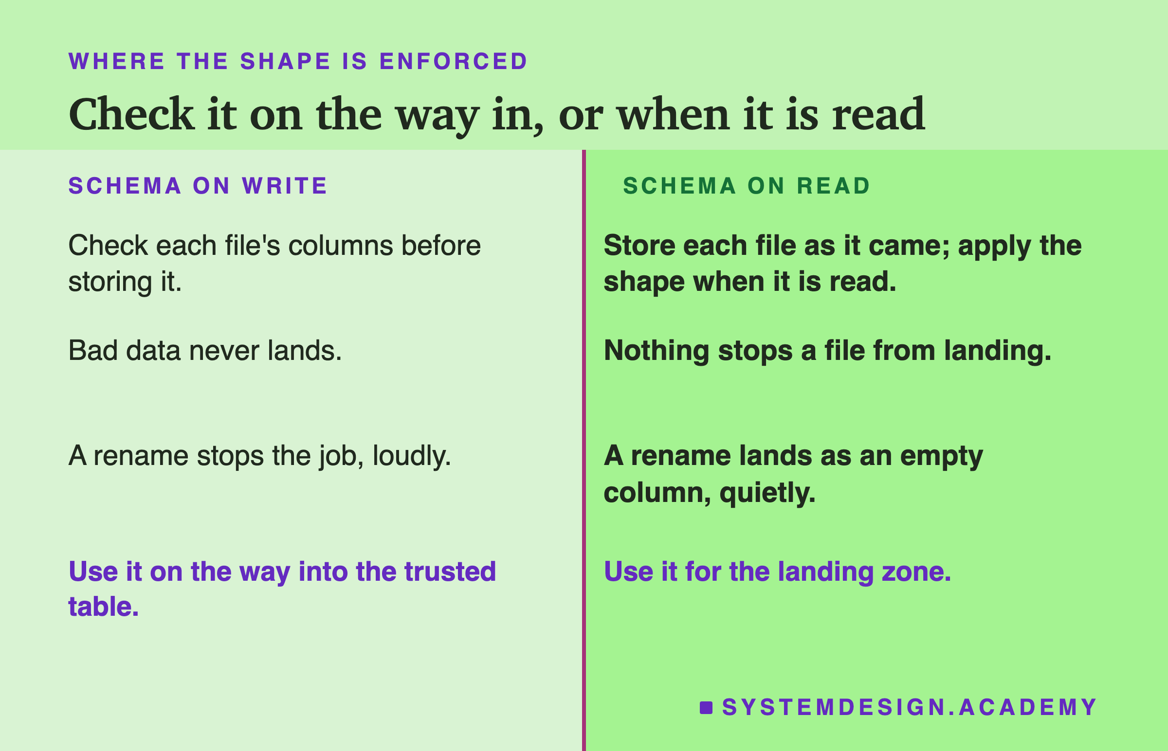
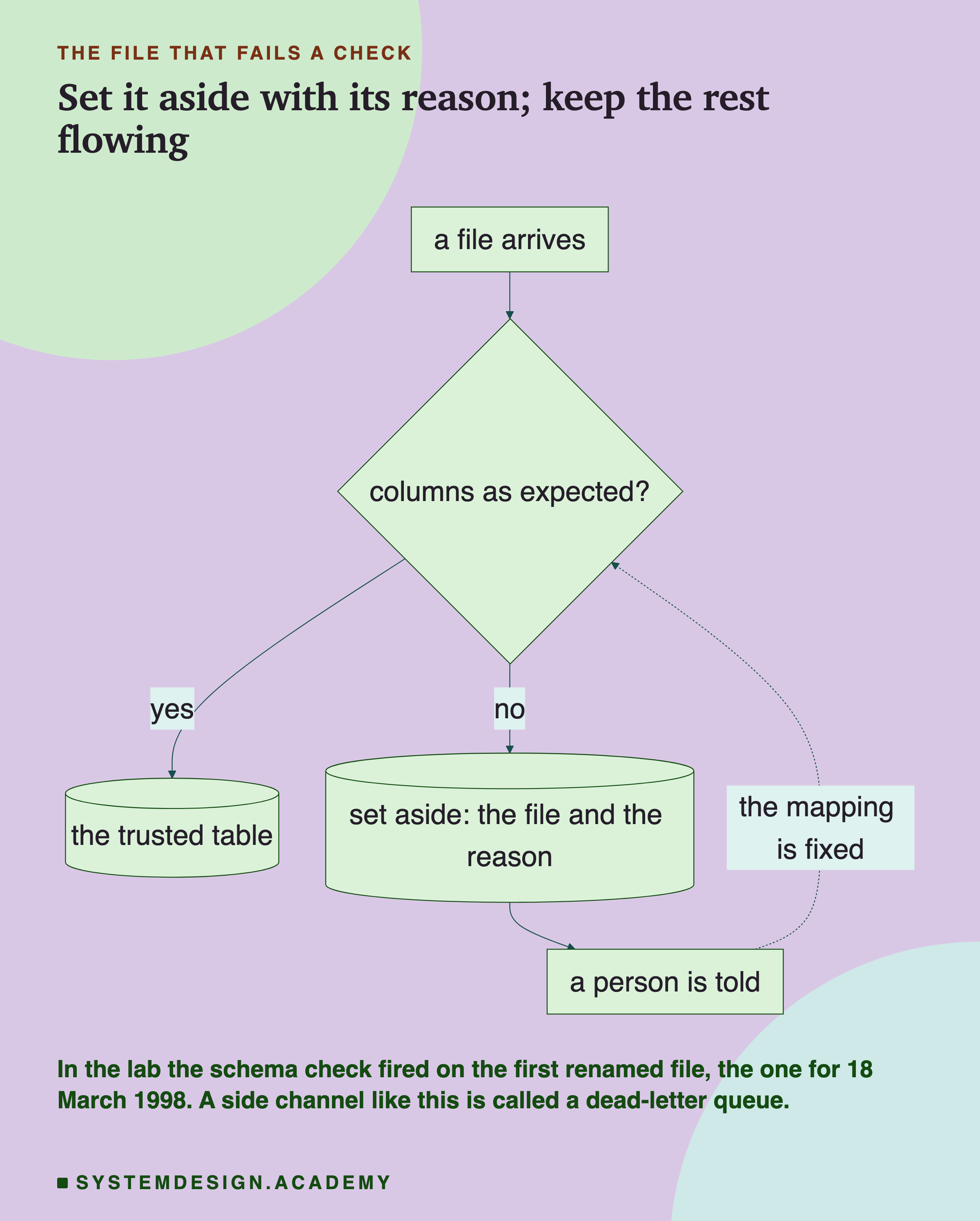
Schema on write checks each file at the door, so a breaking change is caught early, but it stops the pipeline. Schema on read lands everything and applies the shape only when the data is read. Ingestion never stops, but bad data can sit unnoticed in the landing zone. The sturdy answer is to use both, at different layers. Use schema on read into the landing zone, so nothing can stop a raw file from landing. Use schema on write into the trusted table, so no unchecked row is used downstream.

The lab's rename shows why the second half matters. Its job read columns by name with pandas, and pandas does not complain about a missing name. reindex fills it with an empty value, NaN (pandas' documentation: values with no match "are assigned NaN"), and the job then filled that with 0. From the first renamed file on, 3,609 rows had a demand of 0, and nothing failed.

Raw ingested data is honest but messy, so you refine it in layers. Databricks calls this the medallion architecture. In its documentation, bronze "contains raw, unvalidated data". Silver holds "validated, cleaned, and enriched versions of the data". Gold holds "highly refined views of the data" that drive dashboards and machine learning.

In this lesson's terms, bronze is the landing zone. Silver is bronze after removing copies with keyed upserts and checking the schema: the first layer worth trusting. Gold is the features, computed with versioned logic, so a feature means the same thing everywhere it is read. Versioning that logic matters, because the day someone quietly redefines "active user" is the day training and serving stop agreeing.

From gold you publish to a feature store with two copies, fed from the same place. The offline store is for training, and is read over months of history in bulk. The online store is for serving, and returns one user's features in milliseconds. Feeding both from one place prevents train/serve skew, where a model learns from one definition and predicts with another. The course measures it in train/serve skew.

Now the point that ties the first half together. Freshness is decided at ingestion. A nightly batch pull can never give you gold features that are seconds old. However fast the layers above it run, the ceiling was set at the first copy.

Three companies have written about this in their own engineering blogs.

DoorDash built a framework it calls Riviera on Apache Flink, a stream-processing engine. With it, teams describe real-time features in a configuration file. It reads from Kafka and writes to stores including Redis, which powers DoorDash's feature store.

Uber's Michelangelo platform computes some features in batch and some near real time. Its example comes from Uber Eats: a restaurant's average meal preparation time over the last seven days comes from a batch job. The same average over the last one hour comes from a streaming job that reads Kafka.

Netflix carries its event data through Kafka, in its Keystone pipeline. Separately, it wrote that it builds training features from dated snapshots of its online services. That way a model learns from the inputs it would have seen at that moment.

The pattern is the same each time. Pick the ingestion mode that matches how fast the decision must be, and land the data raw. Remove copies with keyed upserts, and absorb bursts with a durable buffer. Correct late windows with backfills, and check the shape at the door of the trusted layer. Only then let it become a feature. The second half of this lesson measures what happens when a pipeline skips some of that.

I wrote the lab's design at the top of its file, scripts/labs/dataeng/ingest_lab.py, before it ran. Everything below comes from its stored results, results/ingest.json, and from a follow-up I designed after seeing them, which the slides mark as such.

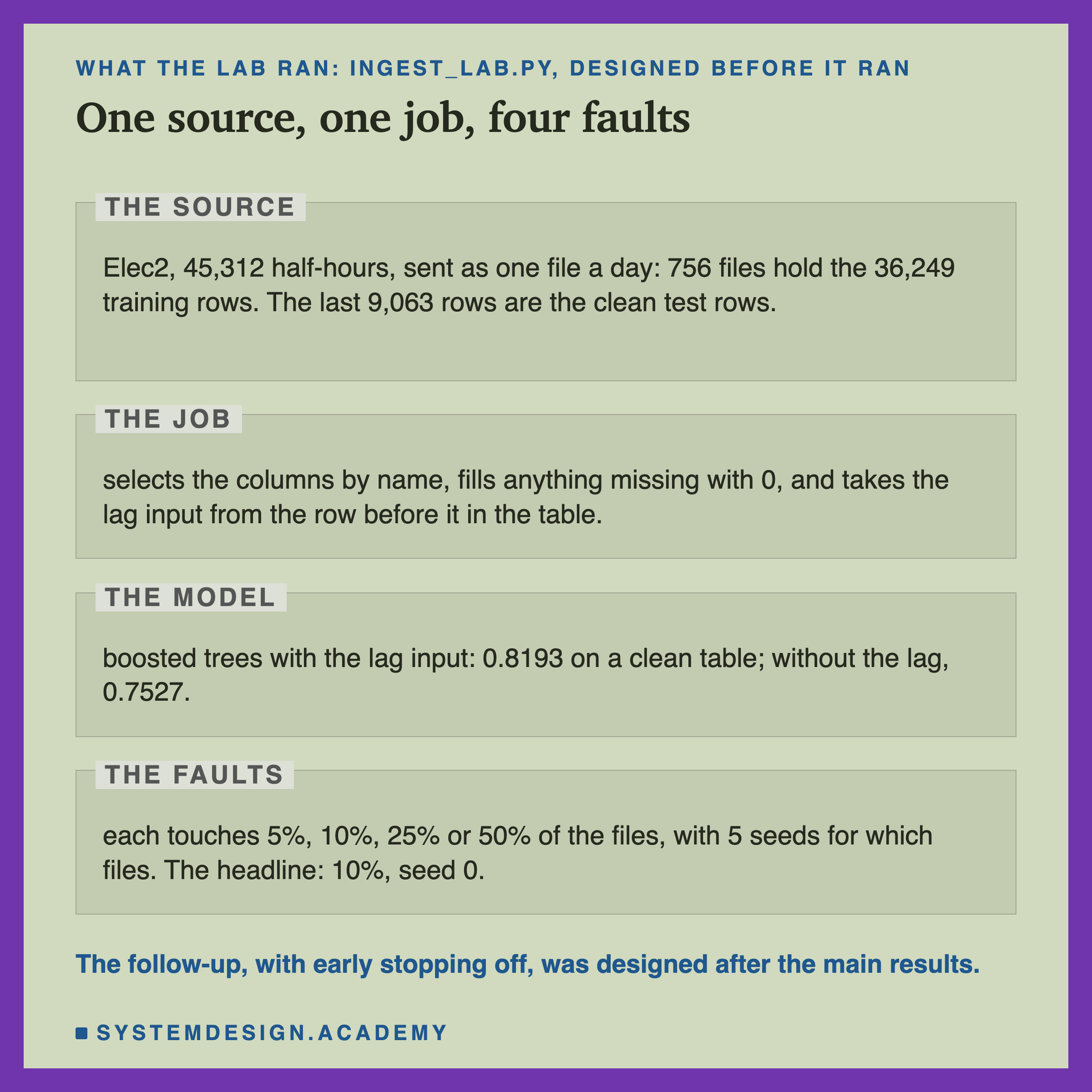
The data is Elec2: 45,312 half-hours of the New South Wales electricity market, from 7 May 1996 to 5 December 1998, 48 a day, in time order. It is small, public and real, and scikit-learn downloads it from OpenML. For each half-hour the label is whether the price went UP or DOWN against its average over the last 24 hours. The first 36,249 half-hours are the training window, and the last 9,063 are the test rows. This is the same split as the lifecycle chapter's lesson on stale pieces in a pipeline, so its numbers can be checked against this one.

The source and the job are a simulation, and I say so plainly. The source sends one file a day: 756 files cover the training window, the last one short. The job is written the way many first versions are. It reads the files in the order they landed, and picks the eight input columns by name. It fills anything missing with 0. It makes the lag input by taking the label of the row above it in the table. In a clean table the row above is the half-hour before, so the lag is right.

The model is a set of boosted trees: many small trees of yes-or-no questions, built one after another, each one correcting the mistakes of the trees before it. It is scikit-learn's HistGradientBoostingClassifier, given the eight inputs plus the lag. On a clean table it scored 0.8193, and the same trees without the lag input scored 0.7527. The first number matches the lifecycle chapter's stored result exactly, and the lab refuses to save anything if it does not.

Here is the training table each fault built, read from results/ingest.json, with each fault touching 10% of the files and seed 0.

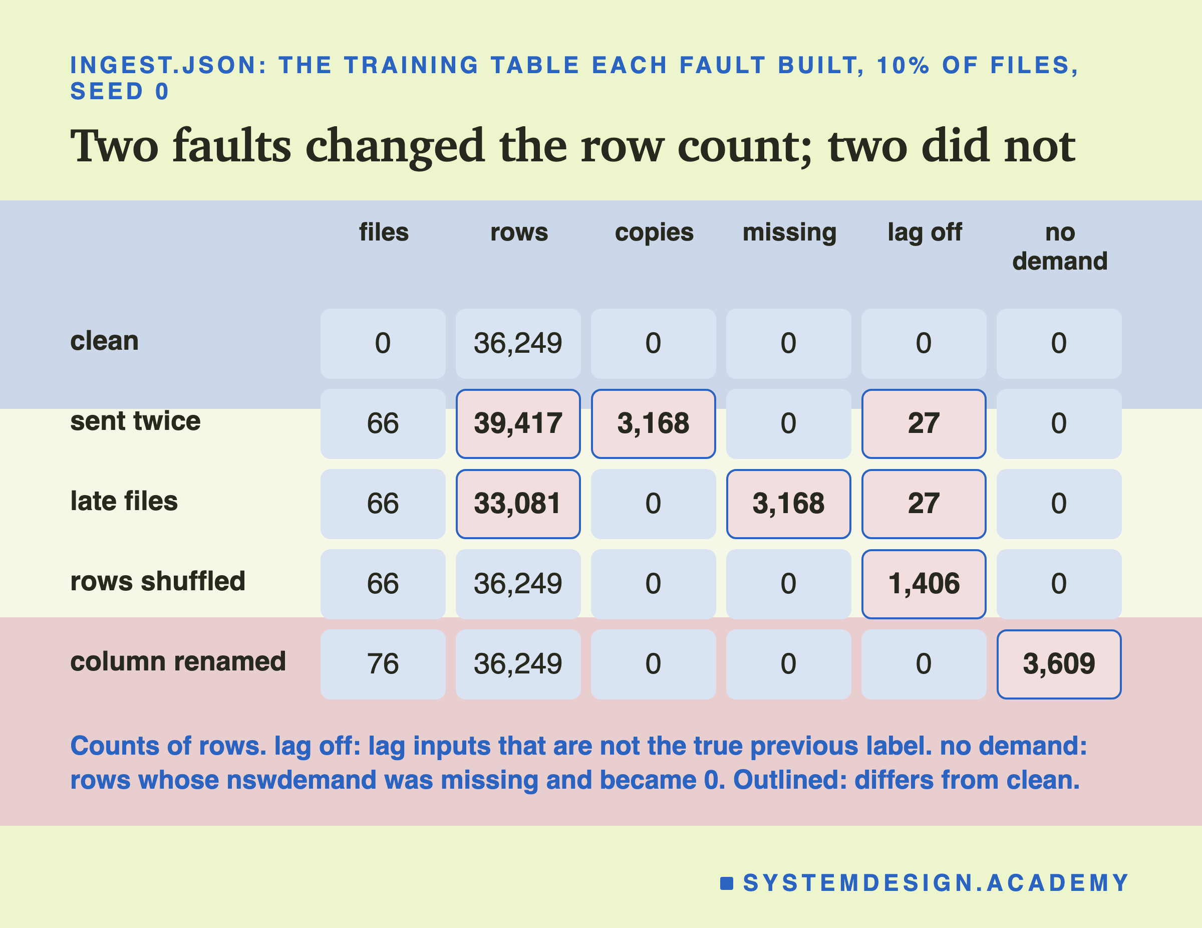
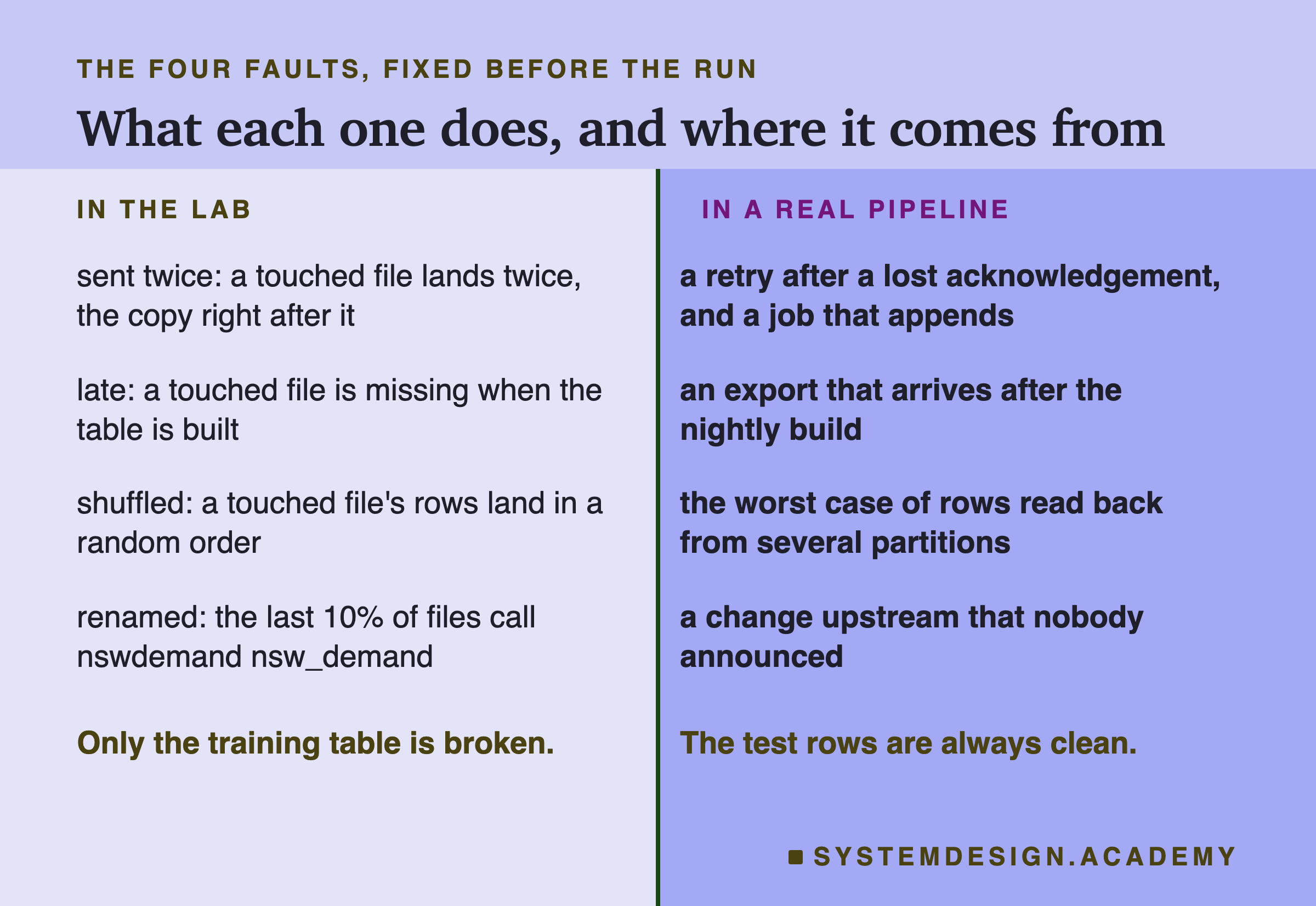
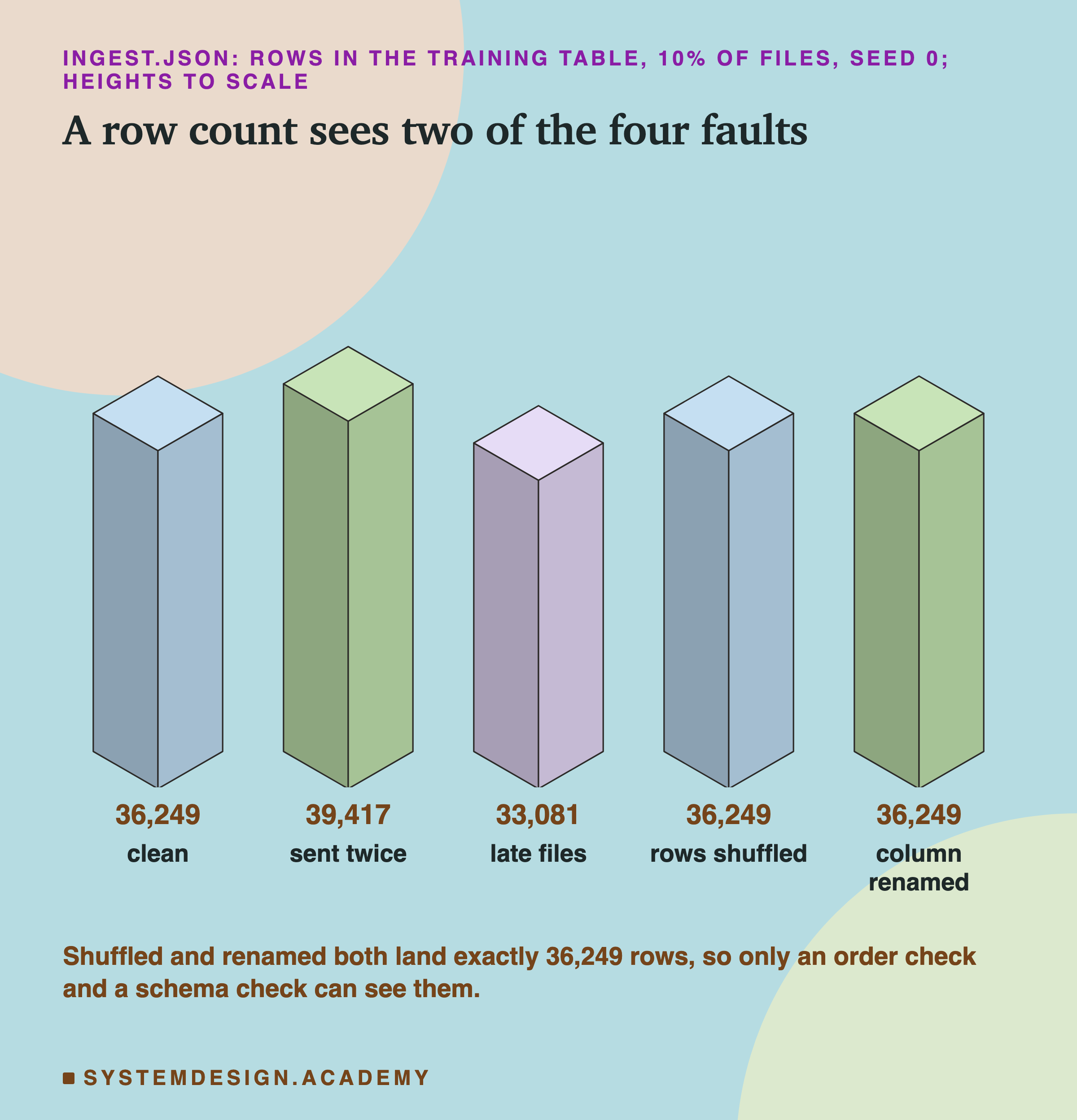
Sent twice landed 39,417 rows for 36,249 records: 66 files came twice, and 3,168 rows were copies. Late files landed 33,081 rows: 66 files had not arrived, and 3,168 records were missing. Both also got 27 lag inputs wrong, at the edges of files. After a copy or a gap, the "row above" a file's first row is not the half-hour before. Rows shuffled landed every row once, but 1,406 lag inputs were wrong. Column renamed landed every row once with every lag right, and 3,609 rows had no demand value, which became 0. The most important number of this slide is not in that table, though.

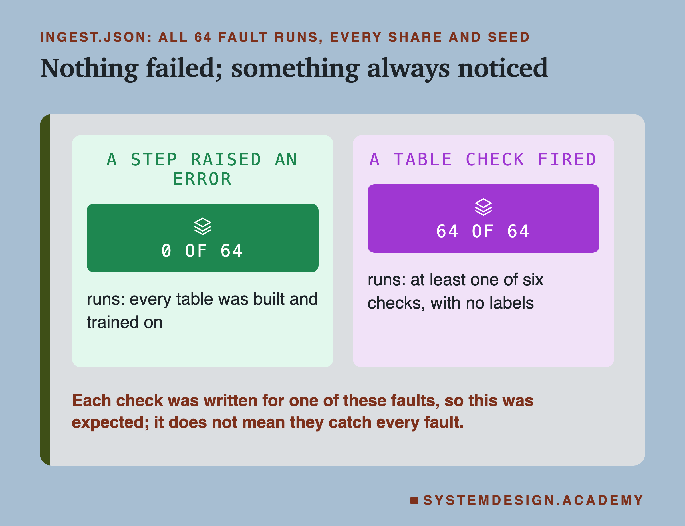
Across all 64 fault runs, every share and every seed, no step raised an error. Every table was built, and every model trained on it; the job did what it was written to do. And in every one of those 64 runs, at least one of six simple checks on the landed files fired. That was expected, since I wrote each check for one of these faults. None of those checks needs a label or a model. It is tempting to think a row count is enough, so here are the row counts on their own.

The shuffle is worth a closer look, because it breaks something the other faults barely touch. Kafka keeps messages in order only within one partition. Its introduction says it "only provides a total order over records within a partition, not between different partitions in a topic". A day's rows spread over several partitions can come back interleaved, though each partition keeps its own rows in order. My simulation puts the rows of each touched file in a fully random order, which is the worst case of that.

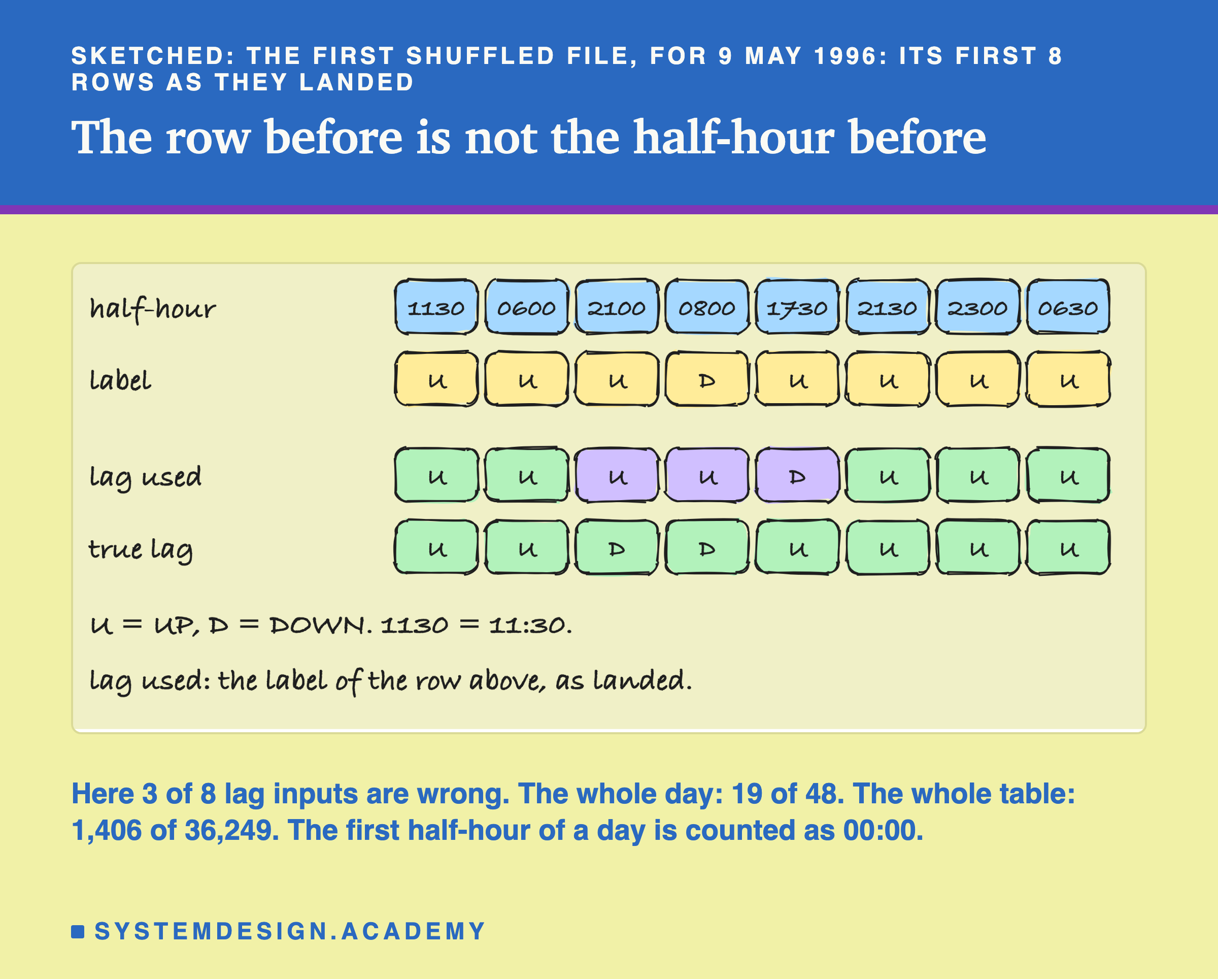
This is the first shuffled file, the one for 9 May 1996. The label of each row is right, and nothing about the rows themselves changed. What changed is the row above each one. The job's lag input is "the label of the row above", which is the half-hour before only if the rows are in time order. Here, 3 of the first 8 lag inputs are wrong; over the day, 19 of 48; over the table, 1,406 of 36,249. As in the lifecycle chapter, the data does not say whether a day's first half-hour starts at midnight, so I count it as 00:00.

The lag input matters because the model leans on it heavily: the trees scored 0.8193 with it and 0.7527 without it. Here is one possible reason the shuffle hurts, which is my reading and not a separate measurement. Taught from a table where the lag is sometimes wrong, the trees learn to trust it a little less. They then pay for that caution on test rows, where the lag is always right. The fix is simple once you see it: build any input that depends on order in key order, never in landing order.

The six checks were fixed in the design, before the run, and each one reads only the landed files. Row count compares each file's rows with the count the source says it sent, its manifest. Copies looks for any key that appears twice. Missing keys looks for any key of the training window that never arrived. Key order looks, in landing order, for a key that is not larger than the key before it. Column names compares each file's columns with the expected list. Empty column looks for an input with no value before the job fills it.

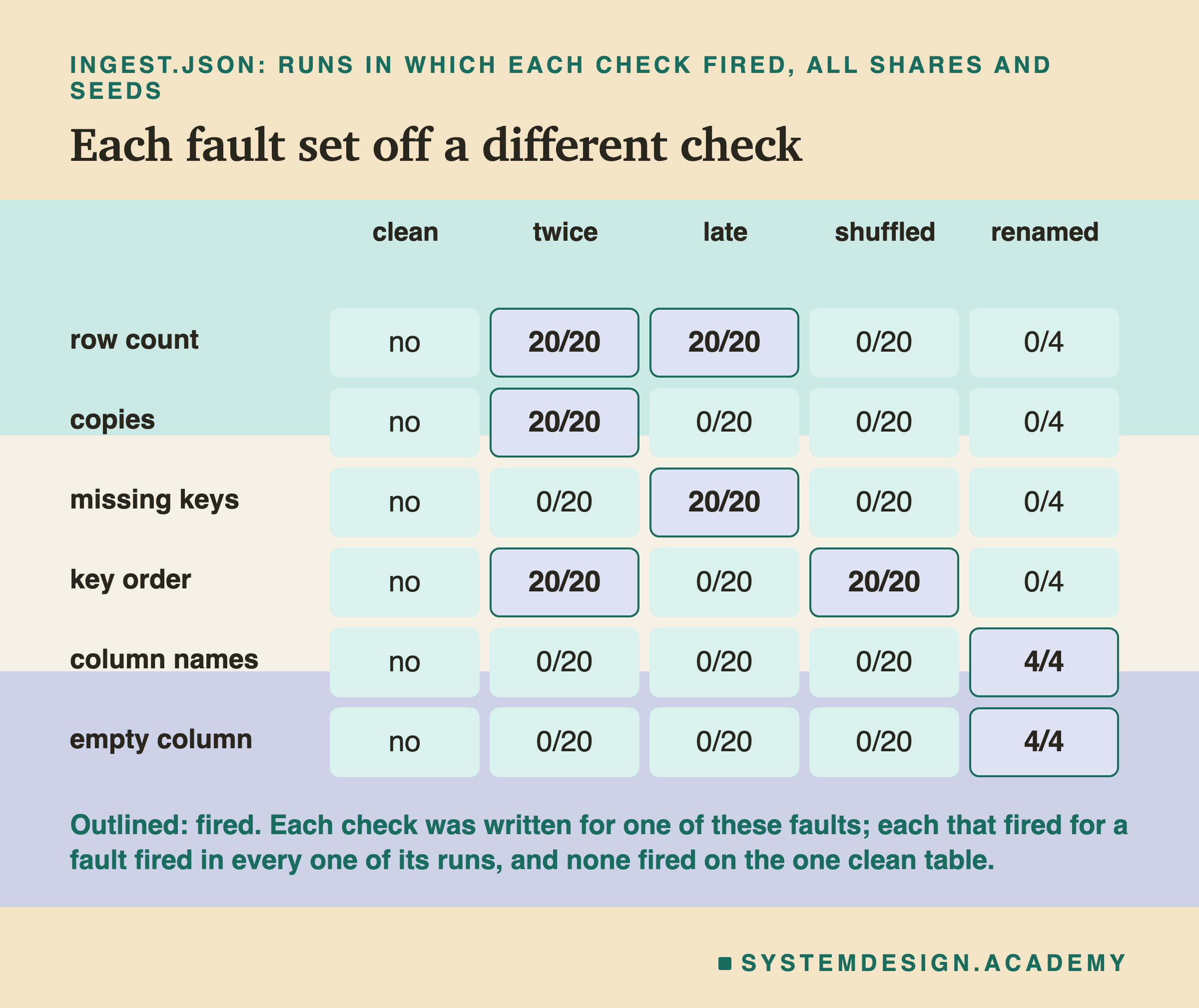
Each fault set off a different check, and each check that fired for a fault fired in every one of that fault's runs, at every share and seed. None fired on the clean table. Sent twice set off the row count, the copy check and key order. Late files set off the row count and missing keys. Rows shuffled set off only key order. Column renamed set off column names and the empty-column check.

Two things follow. First, no single check is enough: the row count, the check teams add first, misses half of these faults. Second, all six together are cheap. Each is a count or a comparison over keys and column names that a pipeline already has in hand. In the lab they need no labels, no model and no waiting for the right answers. So they can run on every file, the moment it lands.

One caution before you trust that table. I wrote each check together with the fault it matches, so each one firing in every run of its fault was expected, not a discovery. The limits slide lists what these six would miss, such as a change of units.

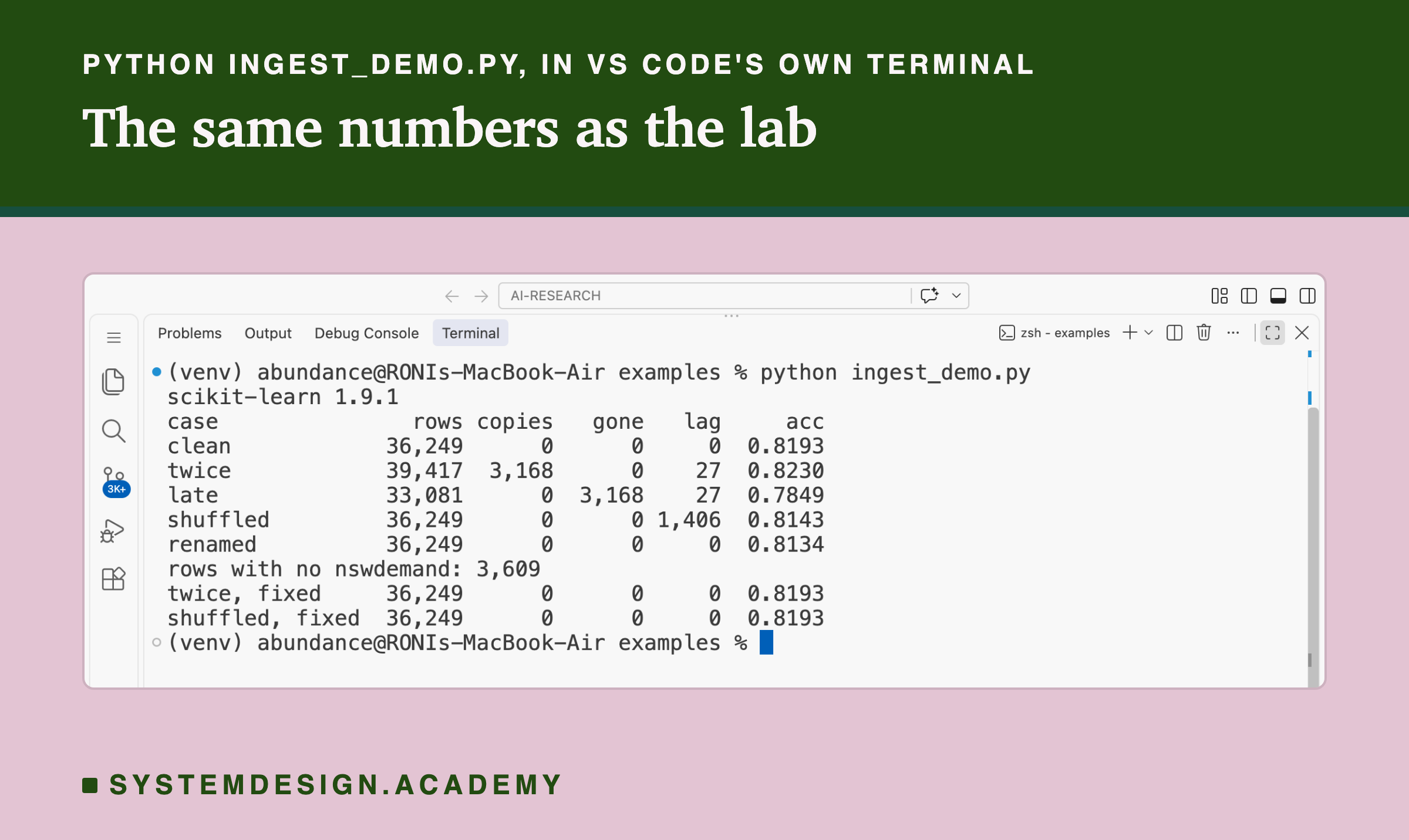
Now the model. For each run the lab trained the same trees on the faulty table and scored them on the 9,063 clean test rows. At the headline, 10% of files and seed 0, the clean trees scored 0.8193. The trees scored 0.8230 with the copies and 0.7849 with the late files. They scored 0.8143 with the shuffle and 0.8134 with the rename. The copies raised accuracy. Before reading anything into that, look at the model on its own.

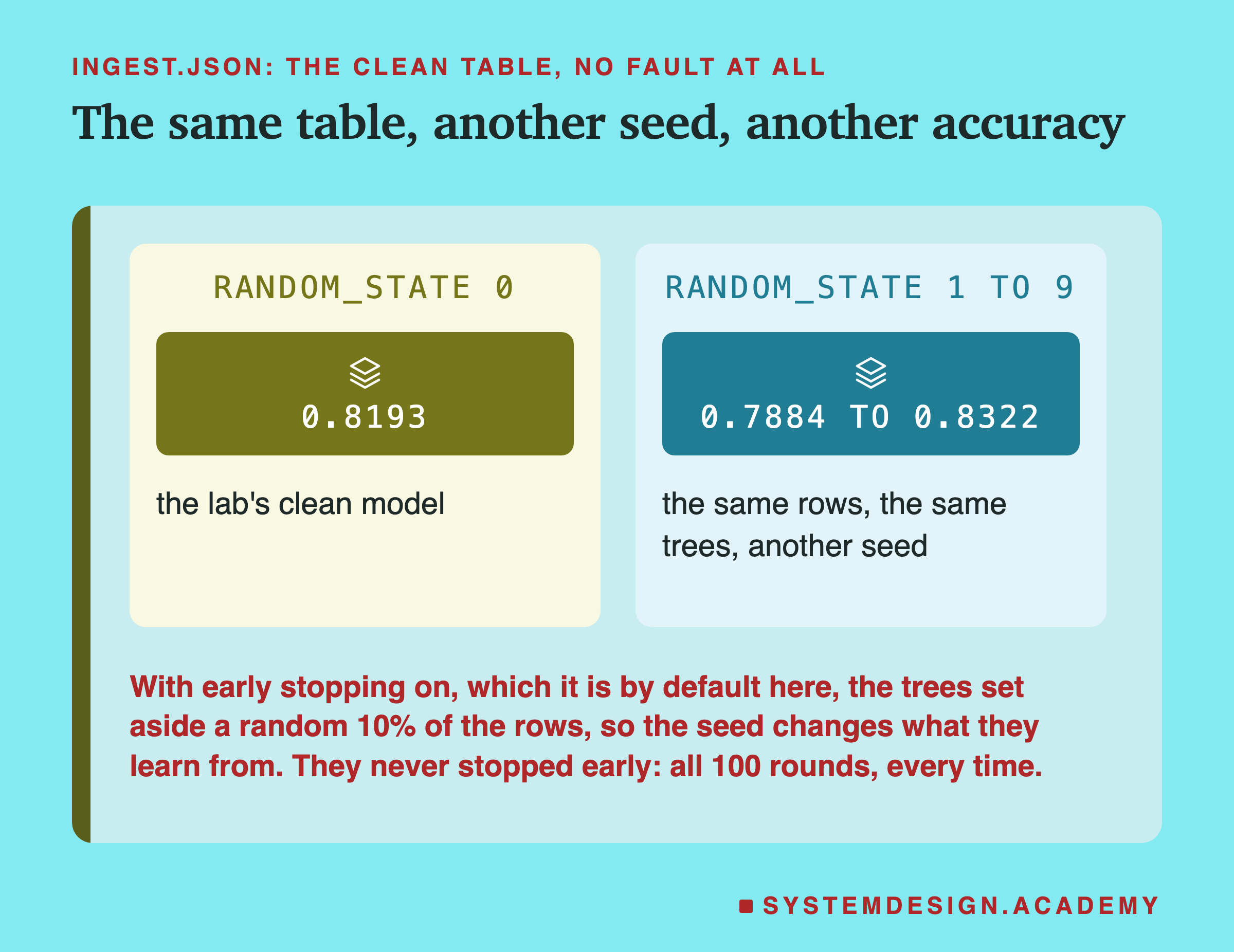
I trained the same trees on the same clean table nine more times, changing only random_state, the seed of the model's own random choices. They scored from 0.7884 to 0.8322, a spread of 4.38 points with no fault at all.

The reason is a default I had not thought about when I wrote the design.

With more than 10,000 rows, scikit-learn's boosted trees turn on early stopping. They set aside a random 10% of the training rows to decide when to stop adding trees, and never learn from those rows. The seed chooses which rows are set aside. So does any fault that changes the number of rows or the order of the labels, because the split is drawn from the row count and the labels. Early stopping itself never stopped early: every model used all 100 of its rounds, so its only effect here was the 10% it set aside.

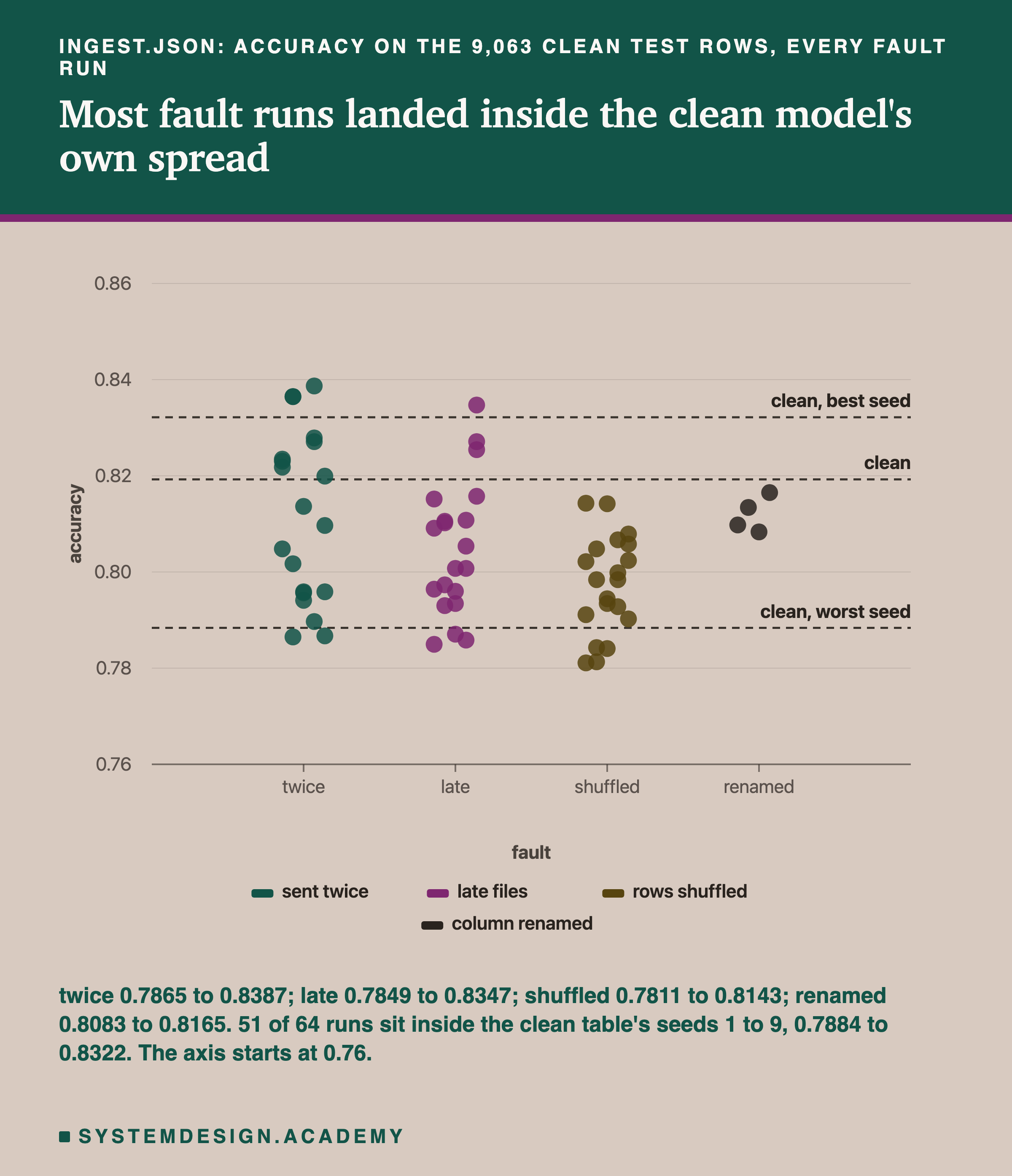
Against that spread, most fault runs look like noise: 51 of the 64 landed inside the clean model's own range. The copies scored above clean in 9 of 20 runs and below in 11. Late files scored below clean in 17 of 20. The shuffle and the rename never scored above clean (the rename had only 4 runs).

After seeing those results, I designed a follow-up, wrote its design into the lab file before it ran, and stored its results in results/ingest_followup.json. It turns early stopping off with early_stopping=False, so the trees learn from every row the job hands over and nothing is left to chance. The lab checked that the new trees give identical answers on a second fit and with another seed. Everything else is the same: faults, shares, seeds, test rows.

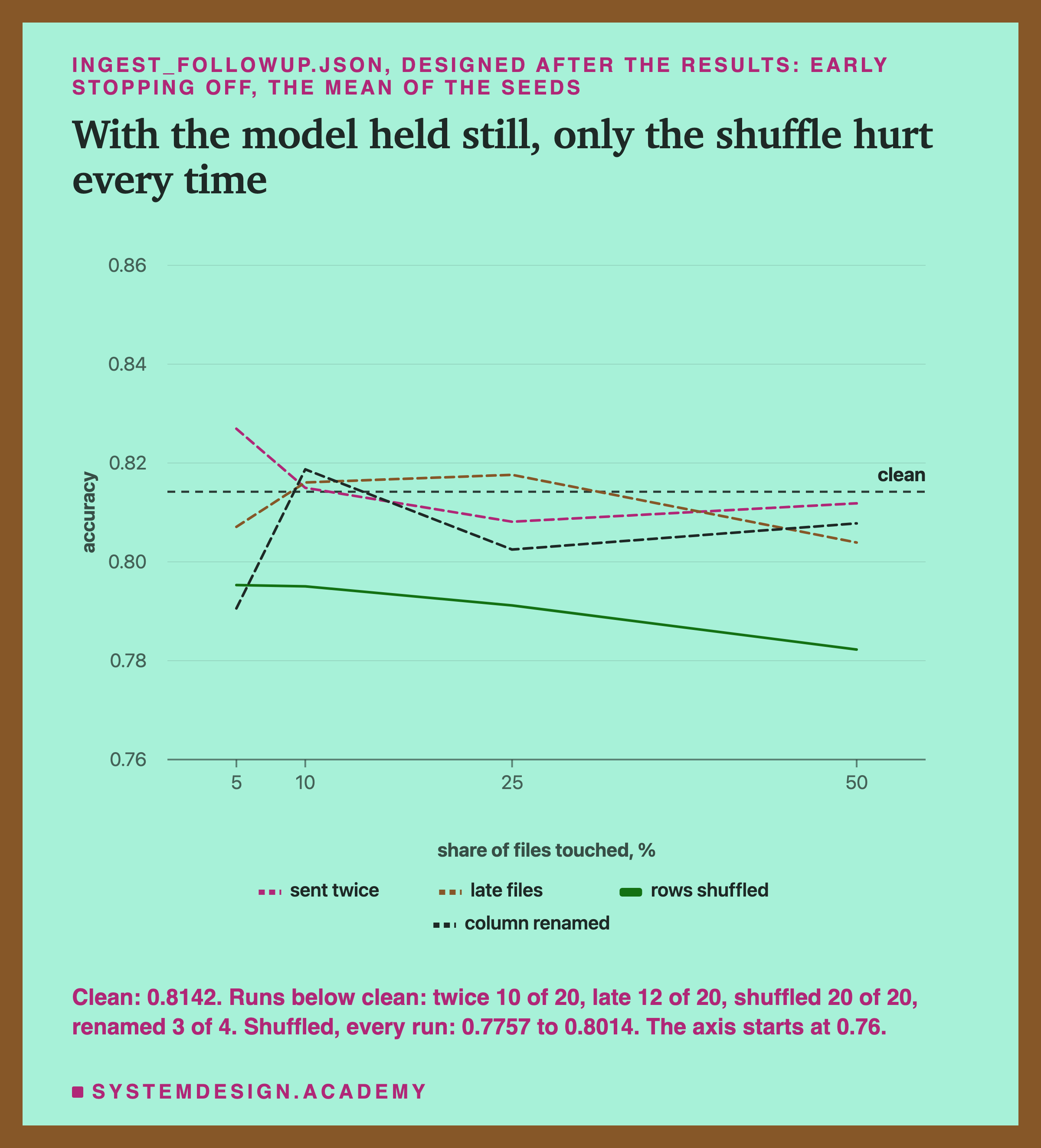
The clean trees now score 0.8142, and 0.7520 without the lag. With the model held still, the picture is clearer, and it is not the one I expected. The copies still went both ways, from 0.7855 to 0.8452, above clean in 10 of 20 runs. Late files went from 0.7705 to 0.8537, below clean in 12 of 20. The rename scored below clean in 3 of its 4 runs. Only the shuffle scored below clean in every one of its 20 runs, from 0.7757 to 0.8014. Its mean falls as the share of shuffled files grows.

How much did each fault change the model's answers? I measured this after the results, from the stored test counts. At the headline, the copies changed 10.5% of the test answers (955 of 9,063 rows). The late files changed 4.2%, the shuffle 3.7% and the rename 3.6%.

Copying 66 of 756 files changed one answer in ten. McNemar's test says the copied model beat the clean one by more than luck, with p far below 0.05. But across five seeds, the same fault made the model better in some runs and worse in others. The test sees that these two particular models differ. The seeds show that the direction depends on which files happened to be copied. The fault did not make models better. It made the model different, in a way nobody chose, and a team watching only accuracy would have called it an improvement.

Each fault has a fix that follows from the first half of the lesson. For copies and shuffles, keep one row per key, in key order, before building any input. For late files, rebuild the day once its file lands, which is a backfill. For the rename, map nsw_demand back to nswdemand; in a real pipeline, the schema check should stop the file until someone does.

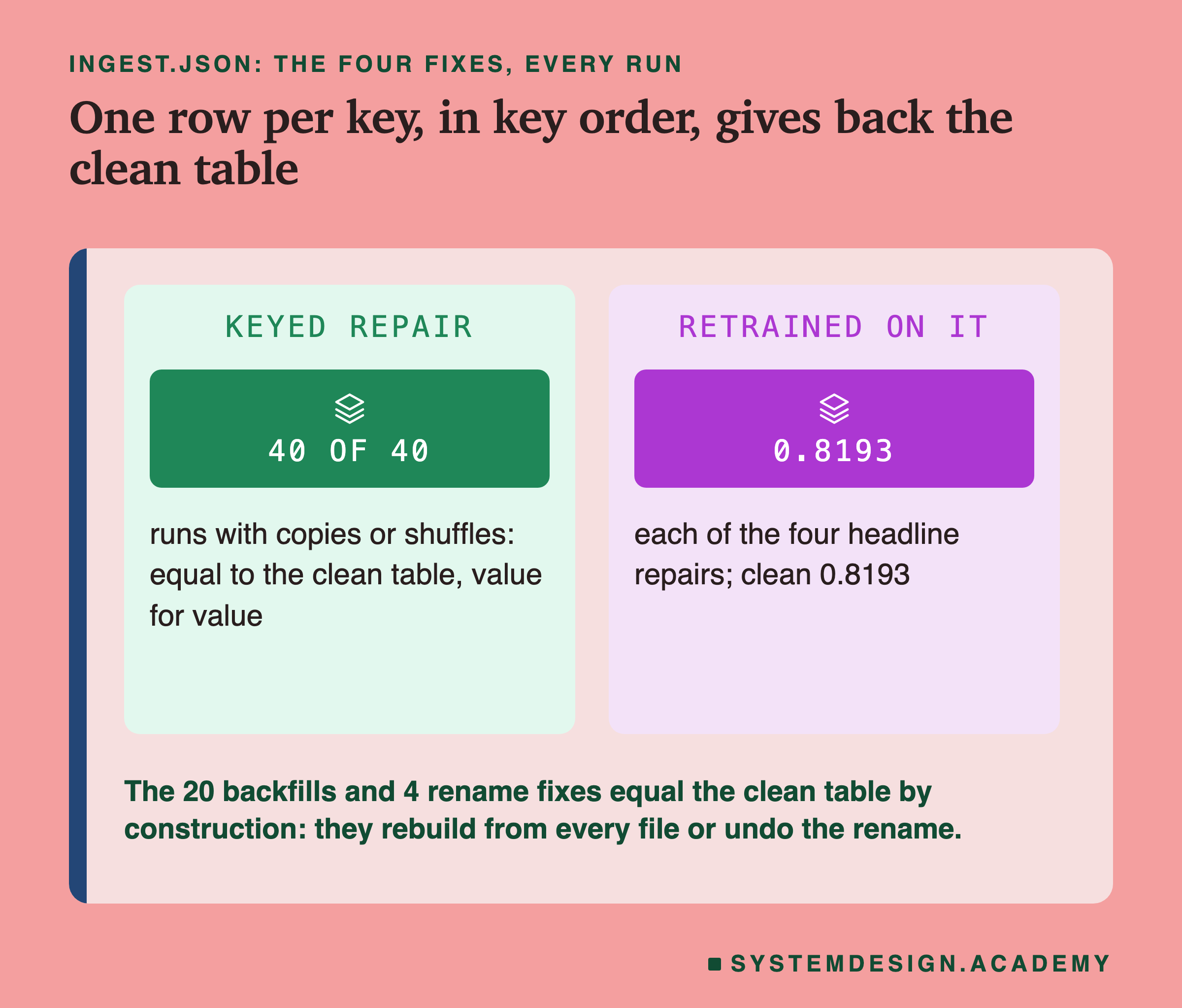
The repairs are not all equally strong evidence. In the 40 runs with copies or shuffles, keeping one row per key in key order gave back a table equal to the clean one, value for value. The lab was written to stop if one was not. That is a real test, and it is idempotency paying off. Because every record has a key, you can repair copies and shuffles without knowing which files went wrong. Sorting by key puts every row back where it belongs.

The other 24 repairs equal the clean table by construction. The 20 backfills rebuild from every file, and the 4 rename fixes undo the rename. A late file or a renamed column cannot be repaired from the table alone: you need the missing file, or someone who knows what the new name means. Retrained, each of the four headline repairs scored 0.8193, the clean accuracy.

This script is the lab made small. It downloads the same data and sends it as one file a day. It applies each of the four faults to 10% of the files with seed 0, and trains the trees on each table. It prints what each table got and what the trees scored on the clean test rows. Then it applies the fix for copies and shuffles. It does not need a GPU.

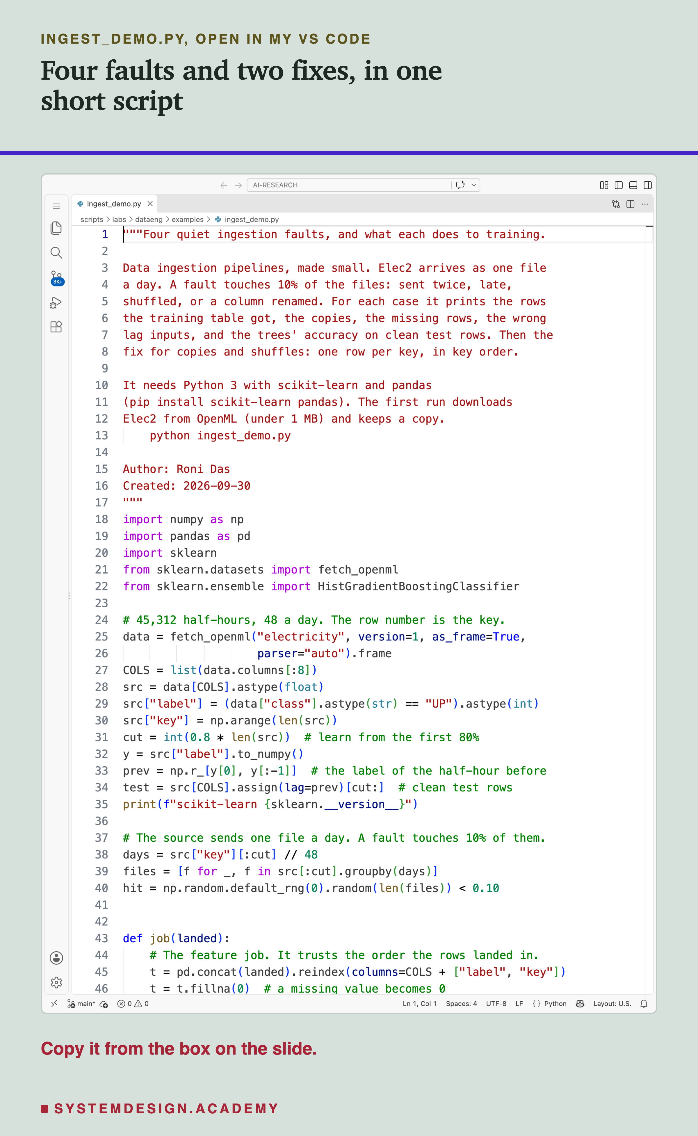
Before you run this lab. You need Python 3 and two libraries: pip install scikit-learn pandas. scikit-learn holds the model and the download, and brings NumPy with it; pandas holds the files and the table. The first run downloads Elec2 from OpenML (under 1 MB compressed), so it needs an internet connection once. scikit-learn keeps a copy in a folder in your home directory (scikit_learn_data) for later runs.

It trains seven small models, so it is quick; I did not time it on a quiet machine. I ran it with scikit-learn 1.9.1 on a Mac. scikit-learn runs the same way on Windows and Linux, but I have not checked the numbers there. Another version of scikit-learn may give different decimals, so the first line printed is the version.

"""Four quiet ingestion faults, and what each does to training.

Data ingestion pipelines, made small. Elec2 arrives as one file
a day. A fault touches 10% of the files: sent twice, late,
shuffled, or a column renamed. For each case it prints the rows
the training table got, the copies, the missing rows, the wrong
lag inputs, and the trees' accuracy on clean test rows. Then the
fix for copies and shuffles: one row per key, in key order.

It needs Python 3 with scikit-learn and pandas
(pip install scikit-learn pandas). The first run downloads
Elec2 from OpenML (under 1 MB) and keeps a copy.
    python ingest_demo.py

Author: Roni Das
Created: 2026-09-30
"""
import numpy as np
import pandas as pd
import sklearn
from sklearn.datasets import fetch_openml
from sklearn.ensemble import HistGradientBoostingClassifier

# 45,312 half-hours, 48 a day. The row number is the key.
data = fetch_openml("electricity", version=1, as_frame=True,
                    parser="auto").frame
COLS = list(data.columns[:8])
src = data[COLS].astype(float)
src["label"] = (data["class"].astype(str) == "UP").astype(int)
src["key"] = np.arange(len(src))
cut = int(0.8 * len(src))  # learn from the first 80%
y = src["label"].to_numpy()
prev = np.r_[y[0], y[:-1]]  # the label of the half-hour before
test = src[COLS].assign(lag=prev)[cut:]  # clean test rows
print(f"scikit-learn {sklearn.__version__}")

# The source sends one file a day. A fault touches 10% of them.
days = src["key"][:cut] // 48
files = [f for _, f in src[:cut].groupby(days)]
hit = np.random.default_rng(0).random(len(files)) < 0.10


def job(landed):
    # The feature job. It trusts the order the rows landed in.
    t = pd.concat(landed).reindex(columns=COLS + ["label", "key"])
    t = t.fillna(0)  # a missing value becomes 0
    lag = t["label"].shift(1).fillna(t["label"].iloc[0])
    return t, t[COLS].assign(lag=lag)


def train(name, landed):
    t, X = job(landed)
    trees = HistGradientBoostingClassifier(random_state=0)
    trees.fit(X, t["label"])
    acc = (trees.predict(test) == y[cut:]).mean()
    copies = t["key"].duplicated().sum()
    gone = cut - t["key"].nunique()
    wrong = (X["lag"].to_numpy() != prev[t["key"]]).sum()
    print(f"{name:<16}{len(t):>7,}{copies:>7,}{gone:>7,}"
          f"{wrong:>6,}{acc:>8.4f}")


k = round(0.10 * len(files))  # the files after the rename
renamed = [f.rename(columns={"nswdemand": "nsw_demand"})
           for f in files[-k:]]
cases = {
    "clean": files,
    "twice": [g for f, h in zip(files, hit) for g in [f] * (1 + h)],
    "late": [f for f, h in zip(files, hit) if not h],
    "shuffled": [f.sample(frac=1, random_state=d) if h else f
                 for d, (f, h) in enumerate(zip(files, hit))],
    "renamed": files[:-k] + renamed,
}
print(f"{'case':<16}{'rows':>7}{'copies':>7}{'gone':>7}"
      f"{'lag':>6}{'acc':>8}")
for name, landed in cases.items():
    train(name, landed)

# No error, no copy, no gap: the renamed column just went empty.
raw = pd.concat(cases["renamed"]).reindex(columns=COLS)
print(f"rows with no nswdemand: {raw['nswdemand'].isna().sum():,}")

# The fix for copies and shuffles: one row per key, in order.
for name in ("twice", "shuffled"):
    rows = pd.concat(cases[name]).drop_duplicates("key")
    train(name + ", fixed", [rows.sort_values("key")])

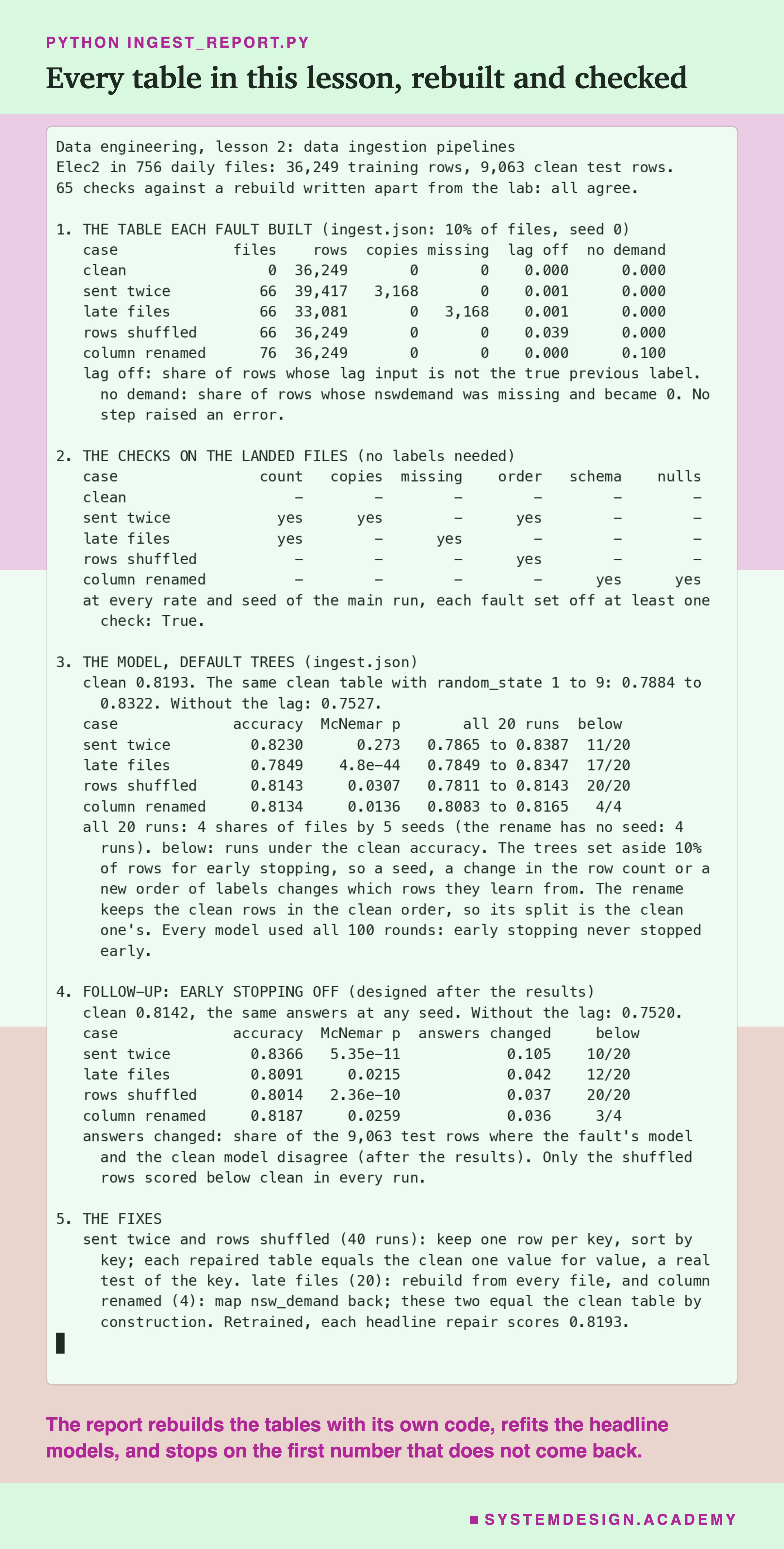
The report lives in scripts/labs/dataeng/ingest_report.py. It reads the lab's two stored files and the Elec2 data from scikit-learn's local copy. It does not trust the lab's code. With its own, separately written code, it lands the files, builds the tables and runs the six checks again. It refits the headline models, and stops on the first number that does not come back exactly. It makes 65 checks, and they all agree. It changes nothing in the lab's files.

Its json mode writes the numbers the figures read to results/ip-report.json. The demo mode checks the student script's stored run. The box mode writes the playground on the next slide and checks it against the lab: 182 checks, at every share and seed the box can rebuild.

What came before the run, in ingest_lab.py: the data, the source and the job, and the model with its two references. Also the four faults, the shares and seeds, the six checks, the fixes, and McNemar's test for the headline runs. What came after I saw the main results: the follow-up with early stopping off, designed and written down before it ran. What came after all the results, in the report: the share of answers that changed, the row counts per file, and the sketched first files.

This box has no model in it. It holds the real labels of all 36,249 training half-hours, and which files each fault touched at every share and seed the lab ran. It also holds the landing order of every file shuffled at 10% with seed 0. From those it rebuilds each landed table and runs the checks, in your browser. The box holds keys, not columns, so its two column checks both read a mark on each renamed file, not real column names. The report checked that every row count, copy count, missing count, share of wrong lag inputs, share of UP rows and check result it gives matches results/ingest.json.

As it is, the box prints the headline table. For each case it shows the rows, copies and missing keys, the share of wrong lag inputs, the share of rows that are UP, and which checks fired. The clean files fire none, and each fault fires its own.

Then try other doses: table(0.50, 3) shows every fault except the shuffle at half the files with seed 3 (the box holds the shuffled order for the headline only). To see copies arrive, print the first key of each landed file with [f[0] for f, _ in land('twice')[:6]]. Try fix('twice') == land('clean') and fix('late') == land('clean'). Last, a question to answer before you run it: at table(0.05, 0), which checks will fire for the late files, and which will not?

Loading. fetch_openml("electricity", version=1) downloads Elec2 once and reads the local copy after that. The first eight columns are the inputs; label is 1 for UP; key is the row number, which names each half-hour. cut is 36,249: the trees learn from the rows before it.

The clean test rows. prev shifts the labels down by one row, so each row holds the label of the half-hour before. test is the last 9,063 rows with that lag added. They are built from the clean source, never from the landed files.

The files. files splits the training rows into one table per day, by key // 48. hit marks the files a fault touches: 10% of them, chosen with seed 0.

job. This is the feature job, and it is where the faults do their harm. pd.concat stacks the landed files in landing order. reindex picks the expected columns by name, and silently gives an empty value for a column that is not there; fillna(0) then turns it into 0. The lag is shift(1): the label of the row above, which is the half-hour before only when the rows are in time order.

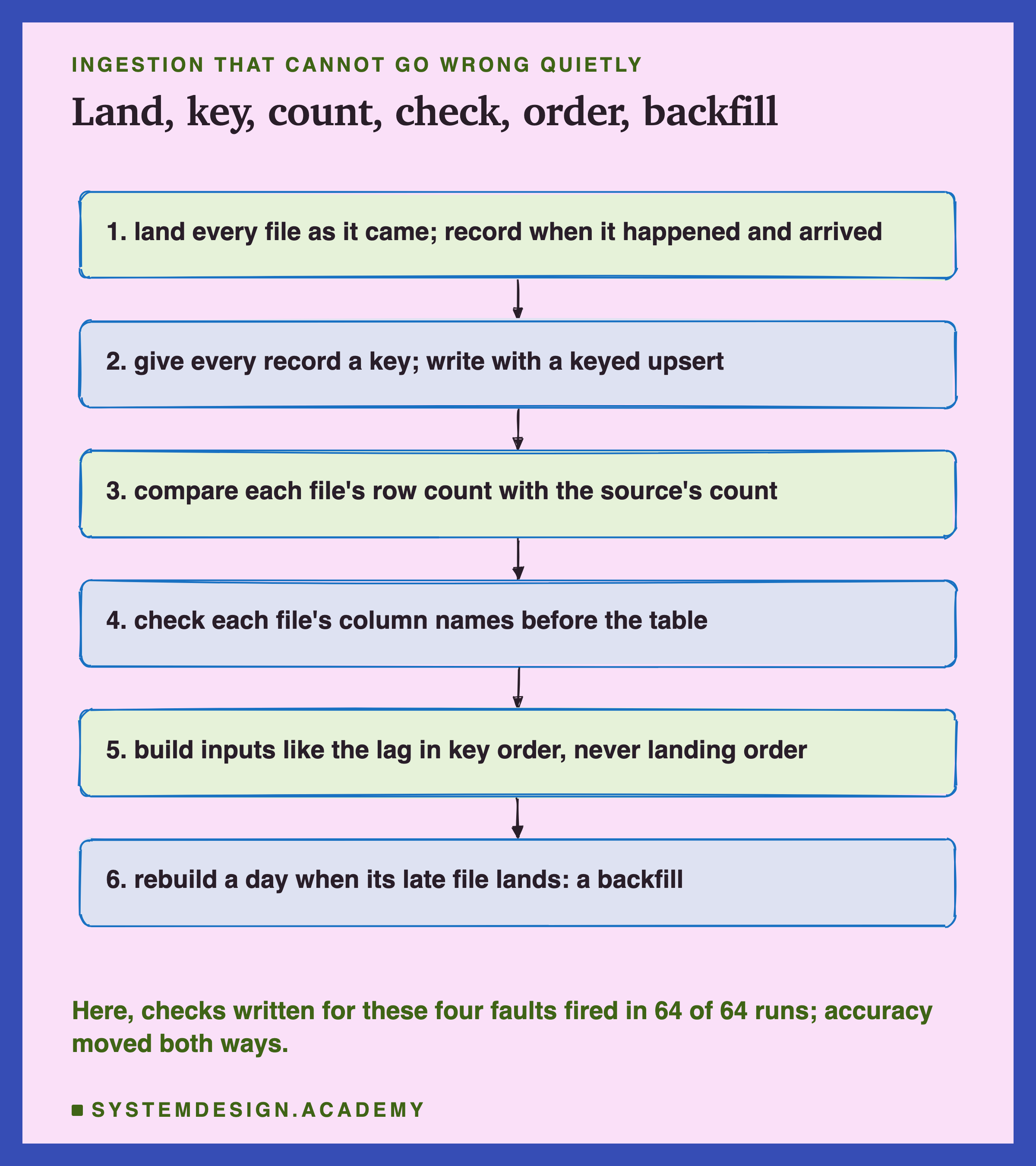
Land every file as it came. Keep the raw copy, and record two times with every record: when it happened and when it arrived. Build time windows from the first. The raw copy is what every later fix is built from.

Give every record a key, and write with keyed upserts. Then a retry, a replay or a backfill cannot create a copy, and a version column decides which copy wins.

Count at the door. Ask the source for a count per file or per day; many exports can write one next to the data. Compare it with what landed. In the lab this caught the copies and the gaps in every run.

Check the columns before the table. Compare every file's column names and types with what you expect, and stop the file, or set it aside, on a mismatch. Never let a missing column quietly become 0.

Build order-dependent inputs in key order. Any input that looks at "the row before", a running total or a time window must sort by event time or key first. Never trust landing order.

Backfill late days. When a late file lands, rebuild the days it belongs to, and keep recent days marked as provisional until the wait is over.

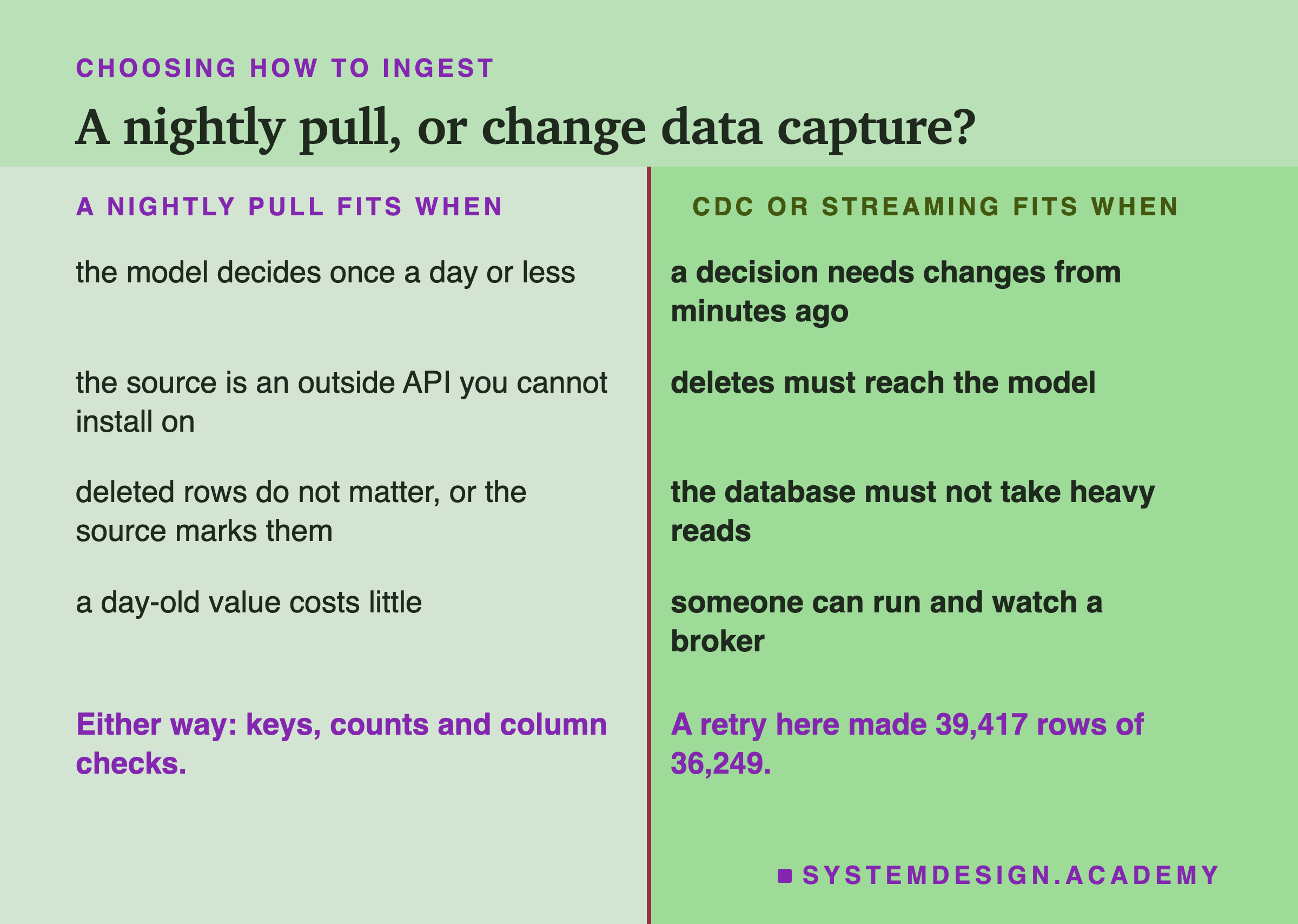
Use a nightly batch pull when the model decides once a day or less. A day-old value costs little there, and a pull is the simplest thing to run and to debug.

Use a pull when the source is an outside API you cannot install anything on. Poll it on a schedule, a page at a time, within its rate limit.

Use a pull only when deletes do not matter, or the source marks them. A watermark on updated_at cannot see a row that is gone, so many teams ask the source to mark a row as deleted instead of removing it.

Do not use a pull when a decision needs changes from minutes ago. Use CDC for a database and streaming for app events.

Do not use a pull when deletes must reach the model, such as a cancelled order or an account whose owner asked to be forgotten. CDC sees deletes; a watermark does not.

Do not run CDC without someone who can run and watch a broker and its replication slots. An abandoned slot can fill a database's disk. And whichever mode you choose, the lab's lesson holds: keys, counts and column checks. Every mode can retry, fall behind or meet a renamed column.

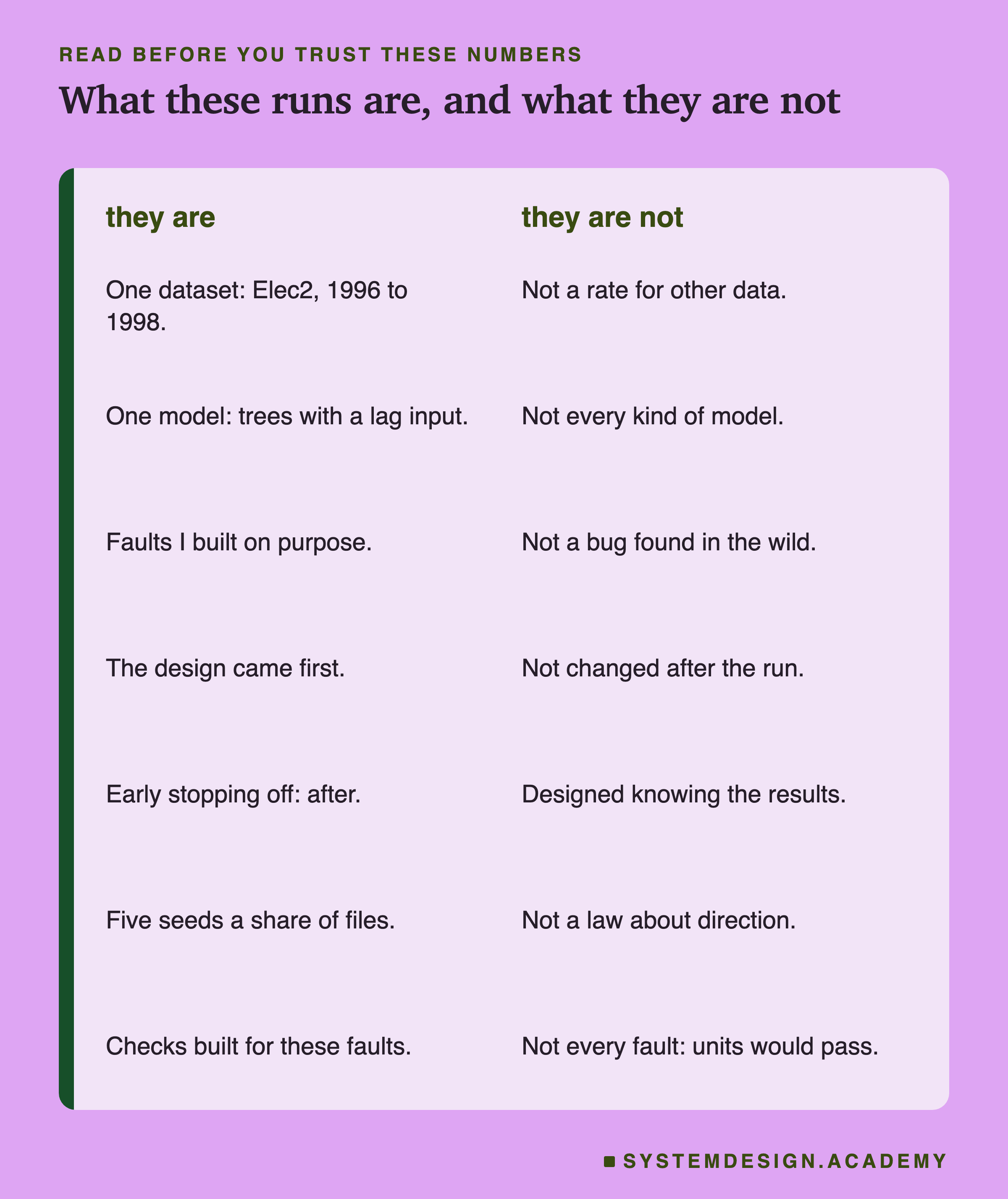
One dataset, one model. Everything here is one electricity market from 1996 to 1998 and one kind of model, boosted trees with a lag input. With other data and other models, what each fault costs would move. The lag input makes this model unusually sensitive to order, which makes the shuffle a clear demonstration and a poor estimate for models without such an input.

Faults I built on purpose. The copies, gaps, shuffles and rename are simulations of failures that happen in real pipelines. They are not a bug I found in someone's system. A real fault can be messier: copies of only some rows, or a rename that reaches only some sources.

Five seeds, not a law. Five seeds per share show the spread; they do not prove a direction. Where I say a fault went both ways, that is five runs, here.

The follow-up came after. Turning early stopping off was designed after I saw the main results, and written down before it ran. The main run's McNemar tests were declared in advance. As the model slide explains, they cannot separate the fault from the change in which rows early stopping set aside.

The checks were built for these faults. I wrote each check together with the fault it matches, so their firing in 64 of 64 runs was expected. "None fired on the clean table" rests on one clean table. The missing-keys check works only because the keys here are row numbers with no gaps. A random id, or an order_id with holes of its own, cannot show a missing record. And a fault none of them was built for would pass all six. If the source began sending demand in kilowatts instead of megawatts, every file would still have the right rows, keys, order and columns.

So do not read this lab as "six cheap checks catch every ingestion fault". They catch these four, and a pipeline needs others too, such as checks on the range and spread of each column. The checks are also strict: any copy, any gap, any key out of order. A real pipeline receives some data out of order for good reasons, so its order check would compare event times within a window. And its row count needs the source to send a count at all.

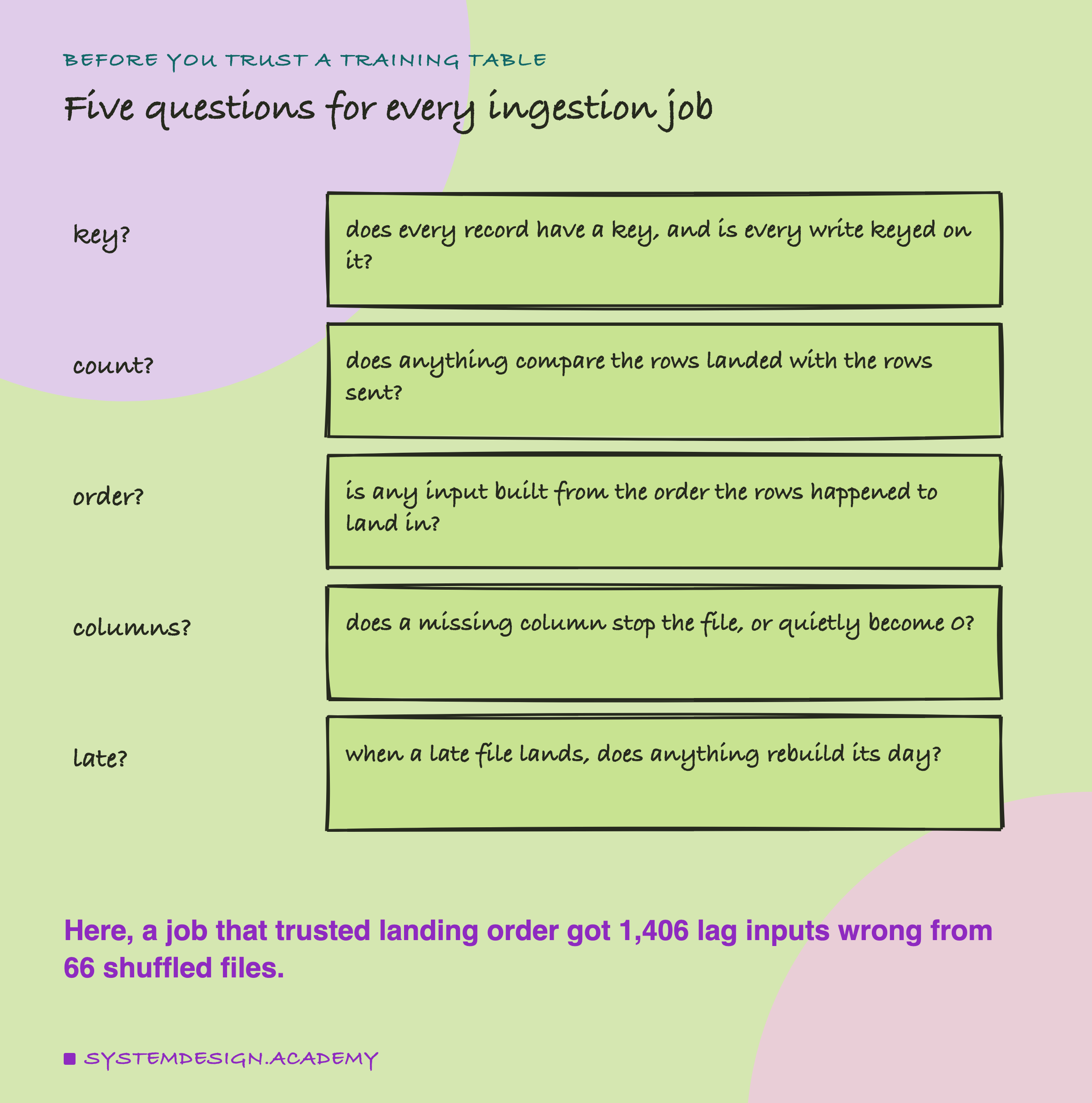
Take one ingestion job your team runs and ask the five questions on the card. If the answer to "key?" is no, start there: a key per record and keyed writes make every later fix possible. If "count?" is no, ask the source team whether their export can write a row count next to each file. It is a small change, and it makes the most common faults visible.

Then run a small version of this lab on your own data. Take one day's landed files, and count the rows per file against what the source says it sent. Then look for repeated keys, and check the key order and the column names. If all four are clean, you have learned something useful about your pipeline. If one is not, you found it before a model did.

The next lesson, ETL vs ELT, is about where the cleaning happens once the data has landed: before it is loaded into the warehouse, or after.

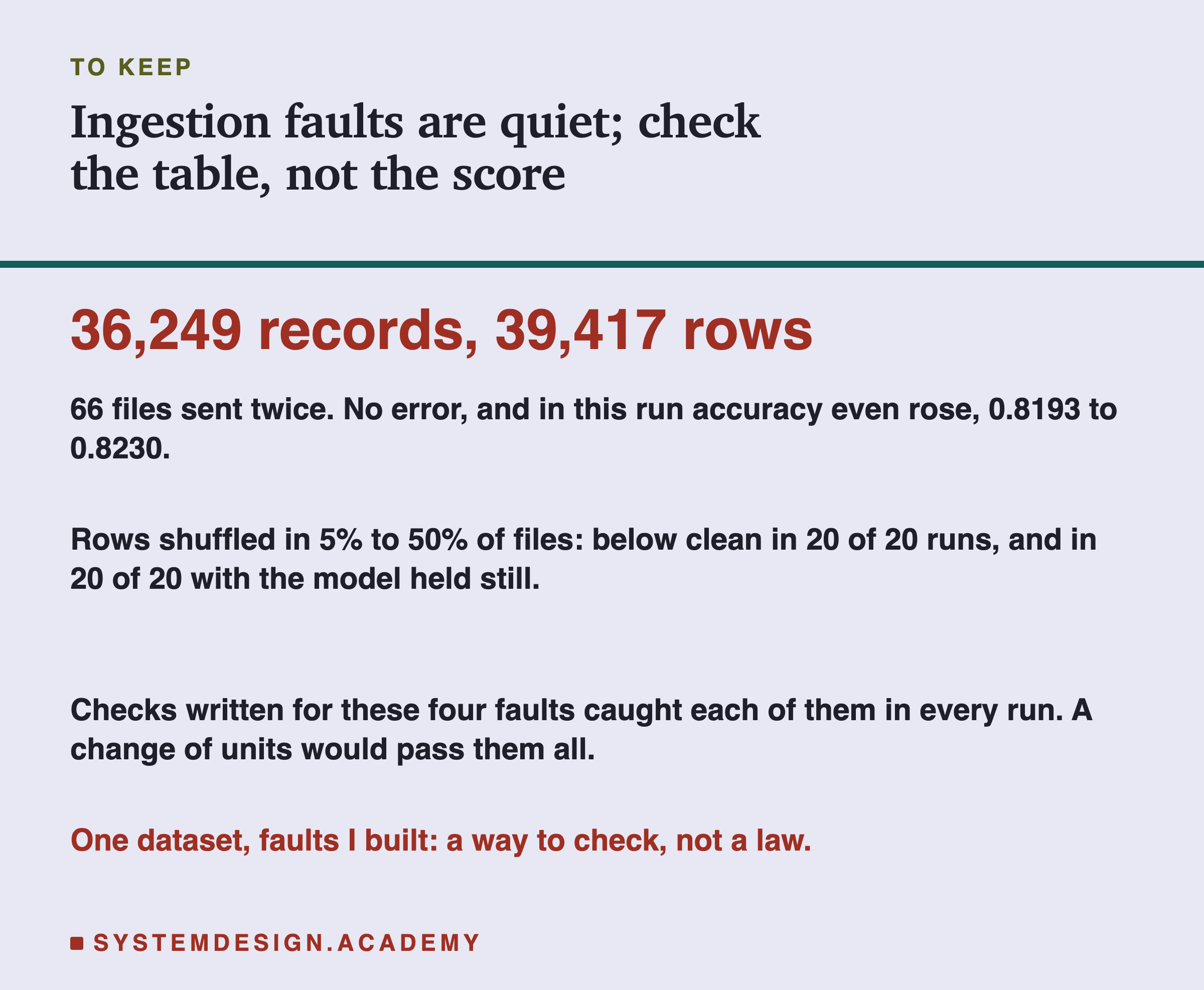
If you keep one thing from this lesson, keep the gap between the two numbers at the top of the card. Those 3,168 copies raised no error, and in that run they even raised the score. A pipeline can be wrong in a way its model rewards, so judge the table by its keys, counts, order and columns, not by the accuracy it produces.