A teacher is getting her class ready for a real exam. She cannot hand out the real paper, so she writes practice questions that look like it. There are three ways this can go.

The first is the good way. The students learn from her practice sheet, sit the real exam, and do well. The practice taught them what the real exam asks.

The second is the vain way. She marks the students on her own practice sheet, sees high scores, and feels good. But she has only learned that the students can answer her questions. She knows nothing yet about the real exam.

The third is the dangerous way. To make the practice as close as possible, she copies questions straight from the real paper. The practice is now perfect, and the real exam has leaked.

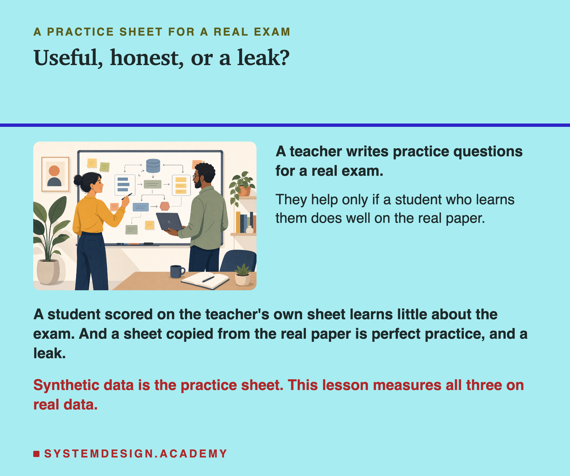
Made-up data for machine learning has exactly these three outcomes. It can teach a model something that works on real people. It can produce a lovely score that means nothing. And it can quietly copy the real people it was meant to protect.

In this lesson I measure all three on a real public table of 30,000 credit card holders. I make the made-up rows myself with three simple methods and train models on them. Then I test those models on real people, and measure how close each made-up row sits to a real one.

This is the ninth lesson of the chapter on data engineering for machine learning. Lesson 8, on handling imbalanced data, was about one label being far rarer than the other. One common fix there, SMOTE, already makes new rows for the rare class. That lesson explains it, so I do not teach it again here.

There is also a lesson in the evals chapter, synthetic cases, about a model writing extra test questions for a search system. It measured that most of the hard cases came from look-alike documents in the collection, which a question generator cannot reach. This lesson is about something else: made-up rows of a table, used to train a model.

What this rebuild corrected. An earlier version of this lesson made claims its sources do not support. Each is fixed where it comes up, and the full record is in results/sdg-factcheck.json.

• It said made-up records with "no real person inside" can be "shared freely". That is unsafe. Data made from people is not private just because it is made up.
• It said a nearest-neighbour distance check "proves" a generator did not memorise anyone. It does not, and the lab below shows a generator passing one such check while sitting on top of real people.
• It said differential privacy is "standard" for synthetic health data. It is not the norm.
• Its TSTR scores (0.89, 0.93, 0.99), its privacy curve, its model-collapse chart and its pipeline counts were made up. They are replaced by measured numbers or cut.
• It said membership inference attacks "pull real records out" of a model. They answer a different question, explained on the privacy slide.

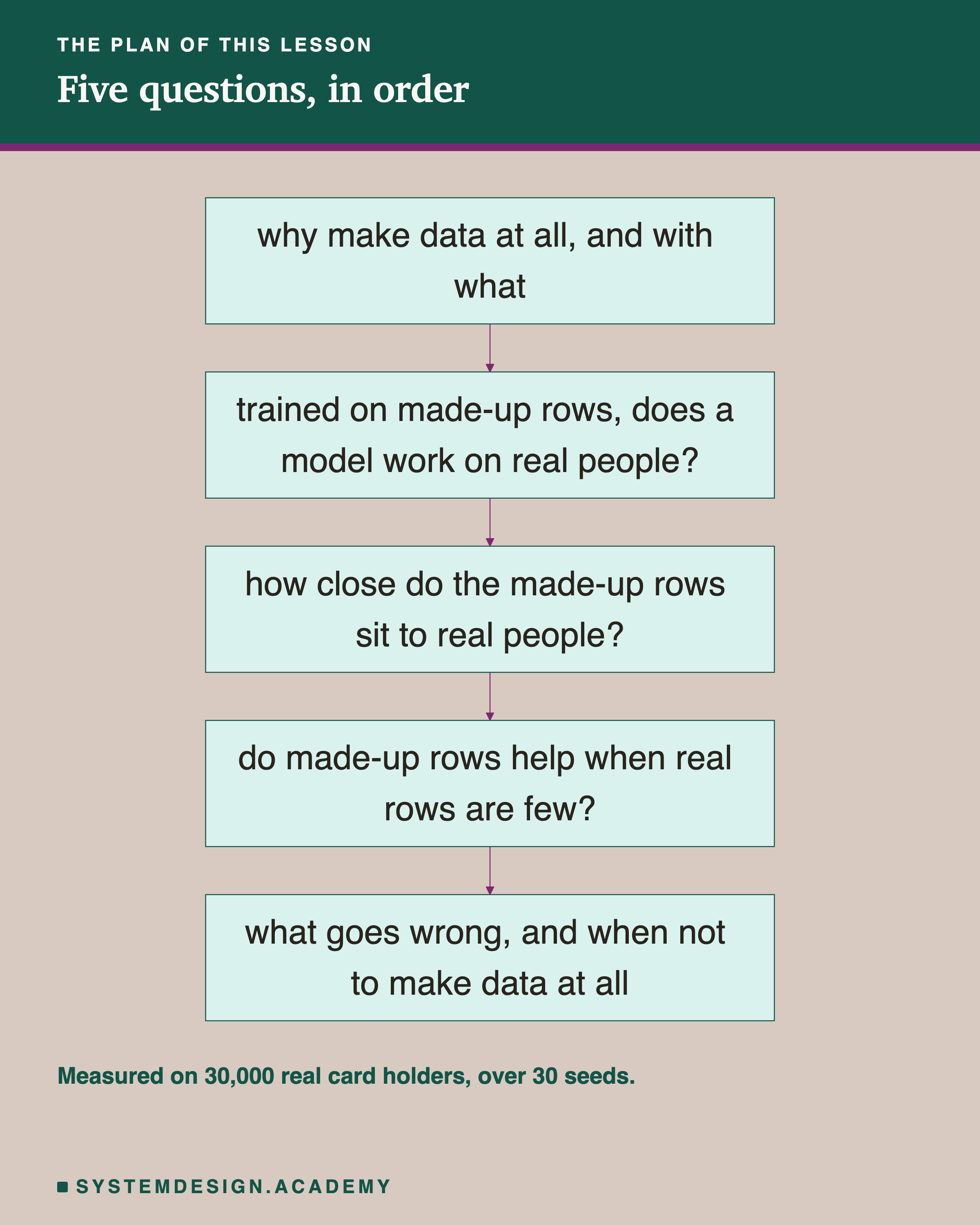
The plan follows the chart from top to bottom. First the reasons and the methods. Then the lab: does a model trained on made-up rows work on real people, and how close do those rows sit to real ones? Then a small test of adding made-up rows to a few real ones. Last, what goes wrong in practice, and when not to make data at all.

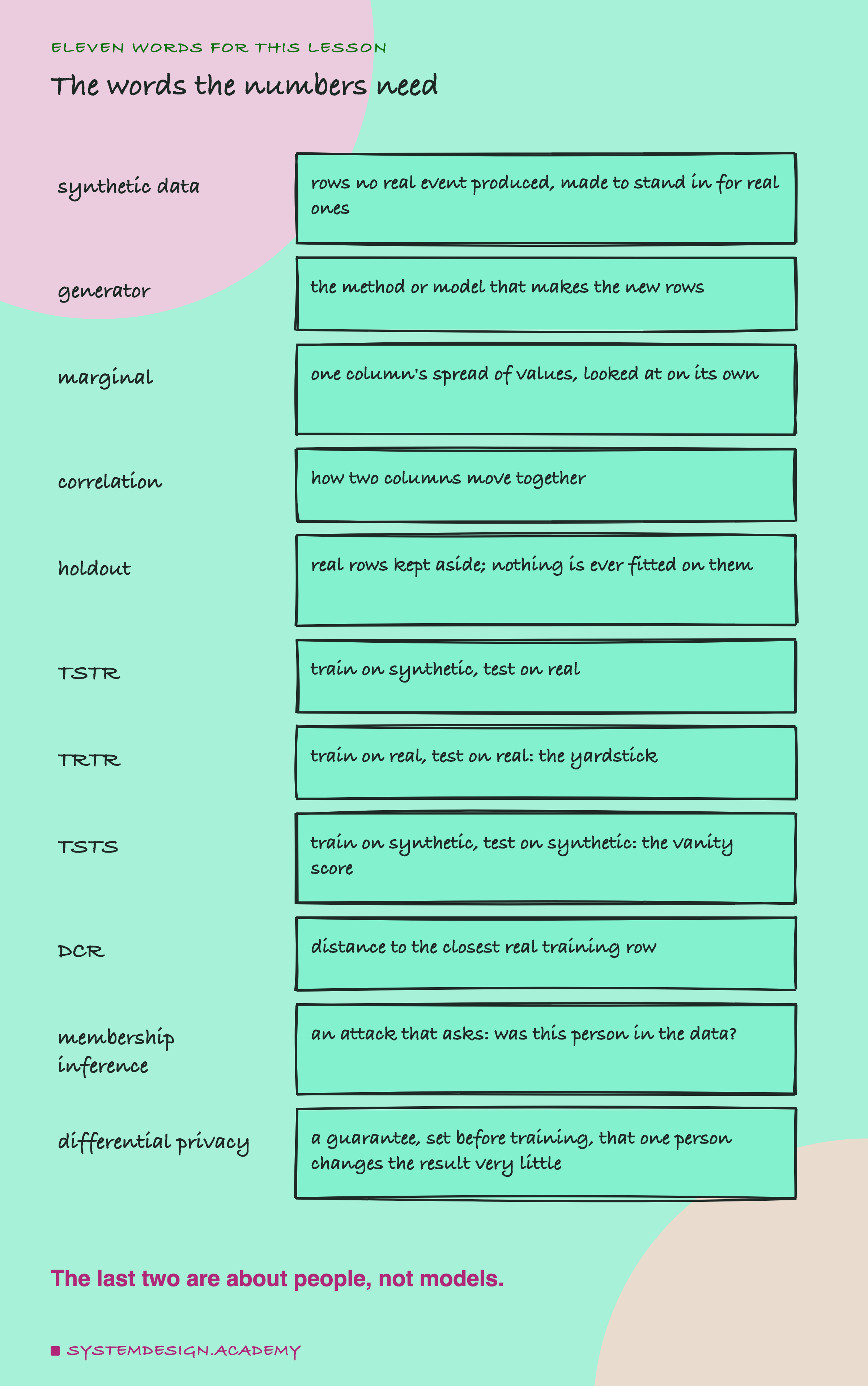
Synthetic data is data that no real event produced. It is made on purpose to stand in for real data. The method or model that makes it is the generator. In this lesson I also call synthetic rows "made-up rows", because that is what they are.

A column's marginal is its spread of values looked at on its own: how many people are 25, how many are 40, and so on. A correlation says how two columns move together. For example, a person's bill this month and their bill last month tend to be close, so those two columns are strongly correlated.

The holdout is a set of real rows kept aside. Nothing is ever fitted on them, so they can act as fresh people the model has never seen.

TSTR means train on synthetic, test on real: train a model only on made-up rows, then score it on real holdout rows. TRTR means train on real, test on real, and it is the yardstick TSTR is compared with. TSTS, train on synthetic and test on synthetic, is the score I call the vanity score, for reasons the lab makes clear.

DCR, distance to closest record, is how far a made-up row sits from the nearest real training row. Membership inference is an attack that tries to tell whether one particular person's record was used in training. Differential privacy is a mathematical guarantee, chosen before training, that adding or removing any one person changes the result only a little.

Synthetic data is a workaround for a shortage, not a free upgrade. When real data is cheap and plentiful, real data wins. You reach for a generator only when the real thing cannot be had in time or at a price you can pay. Teams usually give one of five reasons, and each is a different kind of shortage.

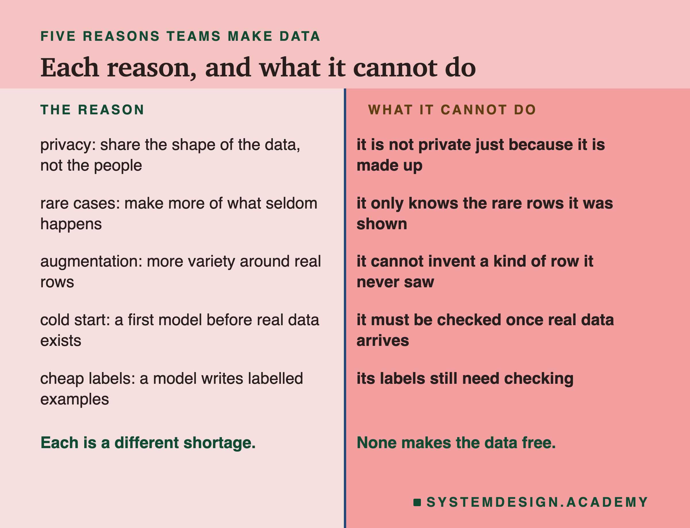
Privacy. You have real patient records or real payments, and you want to share the patterns without sharing the people. This is the most common reason, and the most misunderstood one. A generator learns from the real people, so what it makes can still give them away. The privacy slides below measure that.

Rare cases. The event you care about almost never happens: a crash in fog, a rare disease, a new kind of fraud. A simulator can make as many as you want. A generator that learns from data can only make more of the rare rows it was shown.

Augmentation. You have real data but not enough variety, so you make small changes to real rows to get more. This cannot invent a kind of row you have no example of.

Cold start. A new product has no usage data on day one, so made-up rows let a first model exist. That model must be checked again once real data arrives.

Cheap labels. Paying people to label data is slow. A language model can write labelled examples quickly, but its labels can be wrong and need checking. Lesson 7, on data labeling, measured how labels written by simple rules compare with labels from people.

There is no single way to make synthetic data. The family you pick depends on what you are short of. Here they are from the simplest to the heaviest, with only what a primary source says about each.

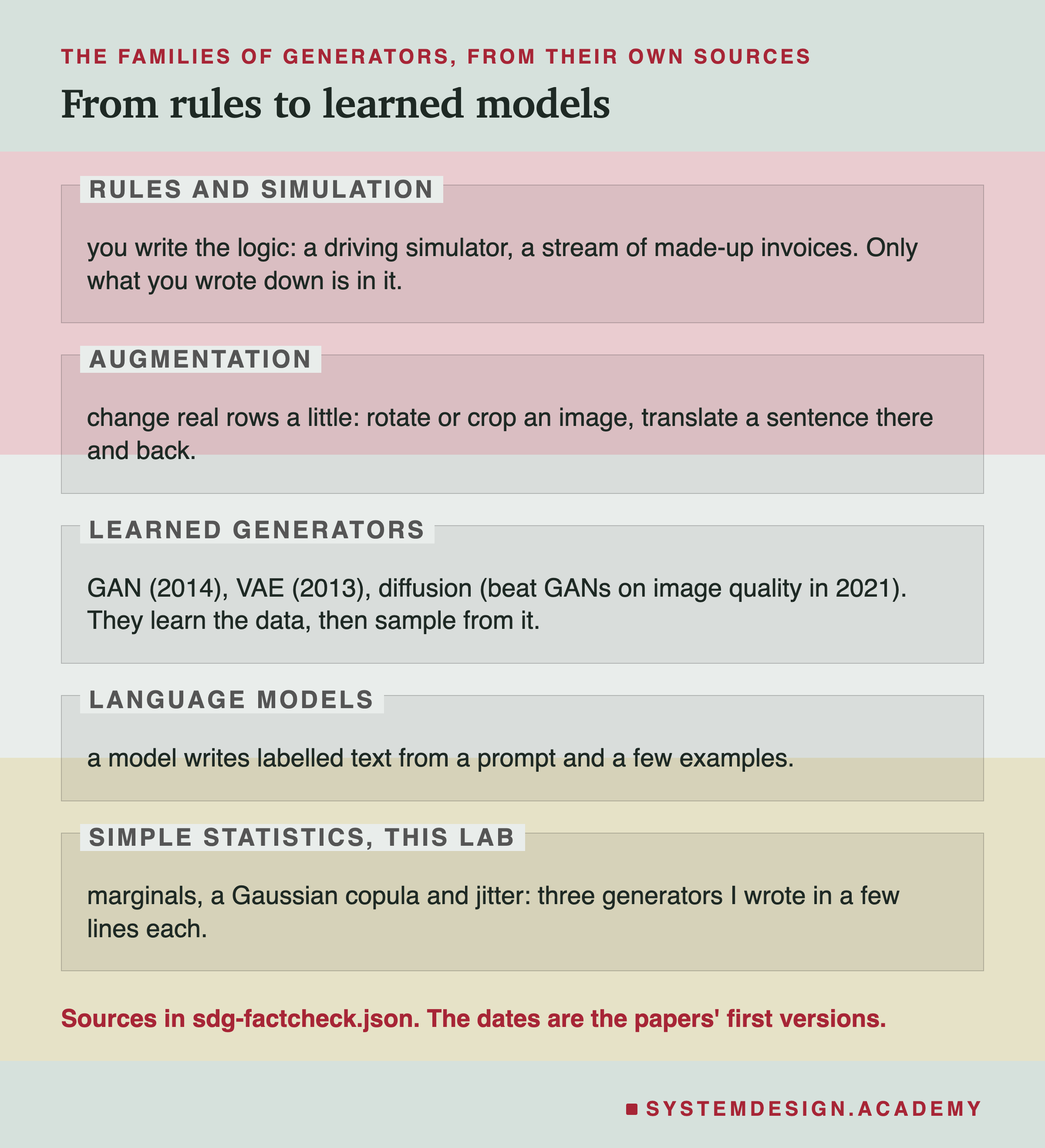
Rules and simulation. You write down the logic yourself: the physics of a road, or the rules of a valid invoice. You get perfect labels and total control over the rare cases. But only what you wrote down is in it, so a pattern you did not think of will never appear.

Augmentation. You take real examples and change them a little. Image libraries such as torchvision, part of PyTorch, ship ready-made changes like random rotation and random cropping. For text, a common trick is back-translation: translate a sentence into another language and back. Sennrich and others used it in 2016 to make extra training data for translation models.

Learned generators. A GAN, a generative adversarial network, is two models trained against each other; the next slide explains it. A VAE, a variational autoencoder (Kingma and Welling, 2013), squeezes each example into a few numbers and learns to rebuild it, so new numbers give new examples. A diffusion model learns to turn random noise into an example step by step. In 2021 Dhariwal and Nichol showed diffusion models beating GANs on image quality. That result was about images, not tables.

Language models can write labelled text from a prompt and a few examples. It is fast, and the speed tempts teams to use the raw output. Remove repeats, check the labels, and test on real examples before you trust it.

The lab uses the last family: three simple statistical generators I wrote myself, so you can see every step.

A GAN, from a 2014 paper by Goodfellow and others, is the classic learned generator, and its idea is worth knowing even if you never train one.

There are two models. The generator turns random numbers into a fake example. The discriminator is a judge: it sees real examples and fakes, and says which is which. Each round, the judge's mistakes are used to improve the generator, and the generator's tricks are used to improve the judge.

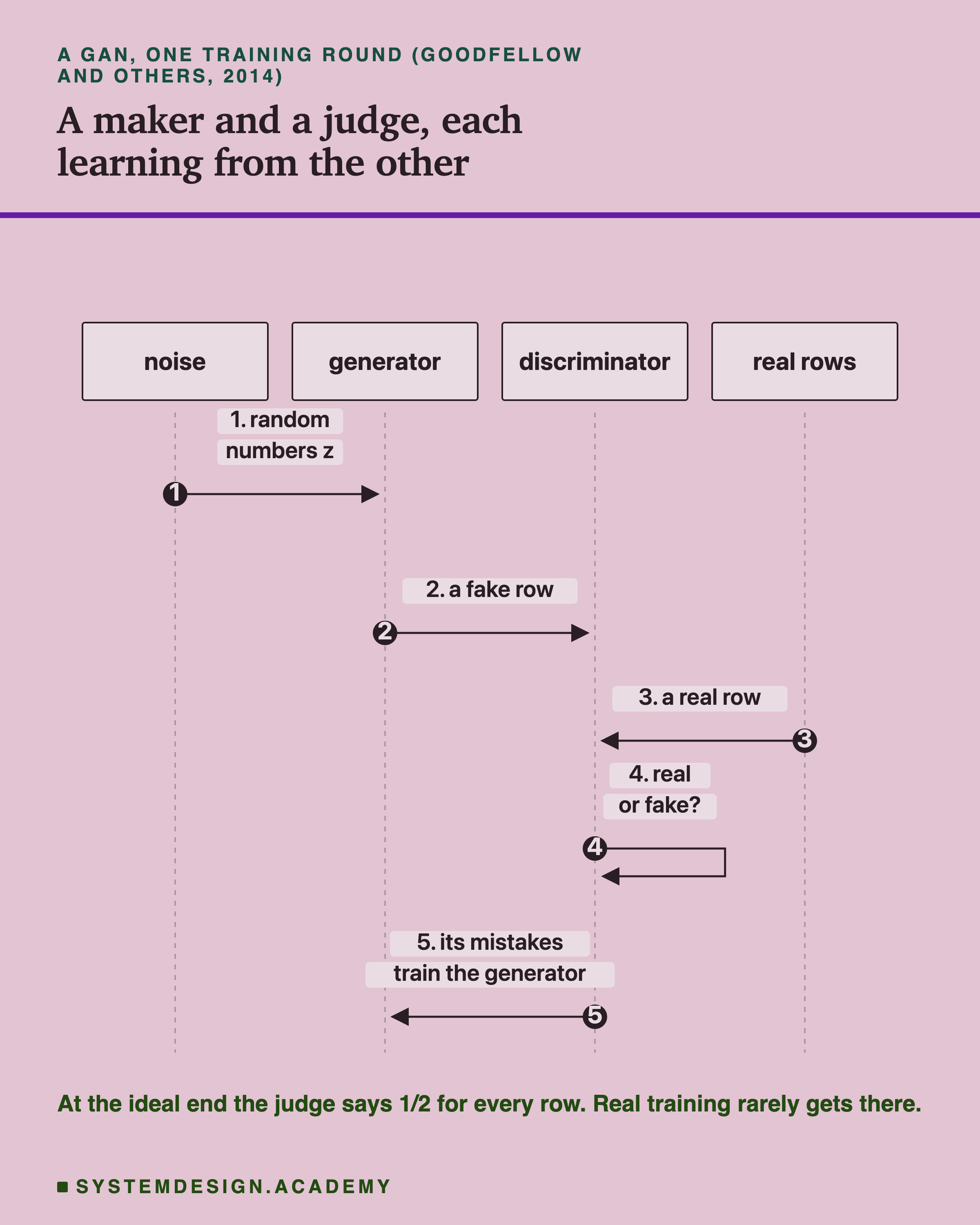
The paper shows how the game ends in an ideal world with unlimited model capacity. The generator copies the data's distribution, the pattern of how often each kind of row appears, and the judge says 1/2, a coin toss, for every example. Real training rarely gets there. A common failure is mode collapse: in the words of Goodfellow's 2016 tutorial, the generator "learns to map several different input z values to the same output point". You get many rows that each look real, with too little variety. The same tutorial says complete collapse is rare and partial collapse is common.

For tables, a well-known GAN is CTGAN, from Xu and others in 2019. It adds tricks for the awkward columns tables have, such as money amounts with several peaks and categories that are rare.

Differential privacy is the formal defence against a generator remembering people. The standard training method, DP-SGD, comes from a 2016 paper by Abadi and others. It cuts down each training example's influence on every update, then adds random noise. The result is a privacy budget written as epsilon (with a small extra term called delta). A smaller epsilon is a stronger promise and usually costs accuracy. Unlike the distance checks later in this lesson, this is a guarantee about every person, chosen before training.

I wrote the lab's design into the docstring of its script, synthetic_demo.py, on 1 October 2026, before it ran. Before writing it I loaded the data once to see its columns and how many people defaulted, and I timed one fit of each model. No score was computed before the design was written.

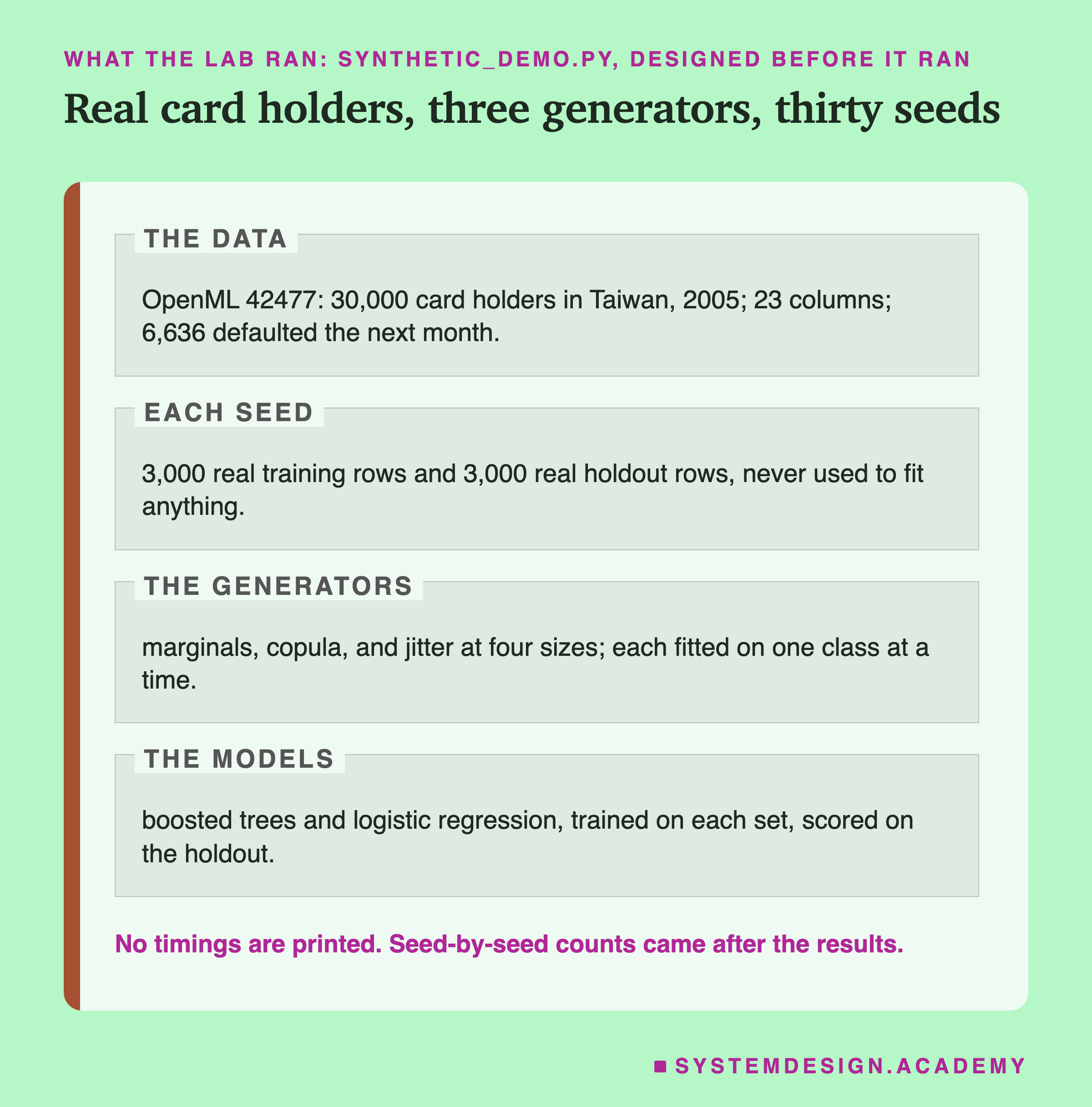
The data is a public table from a 2009 study by Yeh and Lien, published on the UCI and OpenML sites. It holds 30,000 credit card holders in Taiwan, with their payment records from April to September 2005. There are 23 columns: the credit limit, sex, education, marital status, age, then six months each of repayment status, bill amount and amount paid. The label says whether the person defaulted the next month, meaning they failed to pay. 6,636 did, 22.1 percent. I chose it because it is about people. Privacy is the main reason teams make synthetic data, so the test should be on data where privacy matters.

Each seed. A seed is a starting number for the random choices. Each of the 30 seeds shuffles the rows differently. The first 3,000 rows become the real training rows, and the next 3,000 the holdout. One shuffle is one draw, and one draw is not a finding. So every number below is a mean over 30 seeds, with the lowest and highest where it matters.

The models. The lab trains two models on each set of rows. Boosted trees (scikit-learn's HistGradientBoostingClassifier) are many small decision trees, each one fixing the mistakes of the ones before. I switched its early stopping off, so it never quietly holds back part of the training rows. Logistic regression is a simple model that draws one straight boundary between payers and defaulters.

is : the chance that a random defaulter gets a higher risk score than a random payer. 0.5 is a coin toss and 1 is perfect. Lesson 8 explained it in detail.

I did not use a library for the generators, because I wanted every step to be visible. Each one is fitted on one class at a time, payers and then defaulters, and makes as many rows of that class as the training rows hold. So the made-up set always has the same share of defaulters as the real one.

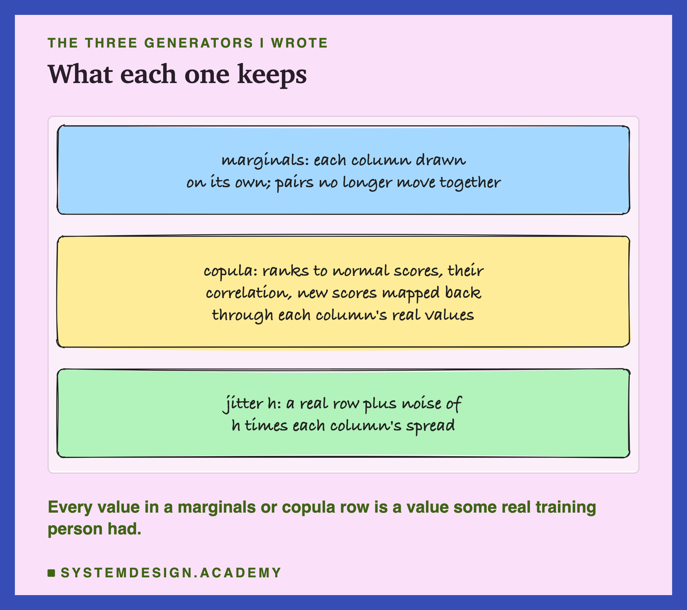
Marginals. For each column, pick a value at random from that class's real values, separately for every column. Each column on its own looks exactly right. But the columns no longer move together: a person's six bills are now six unrelated numbers.

Copula. A Gaussian copula keeps the columns' own values and also the way they move together. It works in three steps. First, each column is turned into ranks, and the ranks into normal scores: numbers that follow the familiar bell curve. Second, it measures how those scores move together. I used a method called Ledoit-Wolf, which gives a steadier estimate when rows are few. Third, it draws new scores with the same pattern and maps each one back through that column's real values. The same idea, in a fuller form, is the GaussianCopulaSynthesizer in the SDV library.

Jitter. Pick a real training row at random and add a little random noise to every column. The size of the noise is h times that column's spread. h = 1 is a lot of noise. h = 0.01 is almost none, so the new row is nearly a copy of a real person. I included jitter on purpose, as a generator I knew could copy people, to test whether the privacy checks catch it.

In every generator, a column with at most 12 different values, such as education or repayment status, is snapped to the nearest value seen in that class.

One fact about the first two generators matters later. Because they only ever pick or map back to real values, every single value in a marginals or copula row is a value some real training person had. The combination is new. The values are not.

The honest test of made-up rows is TSTR, train on synthetic and test on real. Esteban, Hyland and Rätsch named it in a 2017 paper on medical data: "We call it 'Train on Synthetic, Test on Real' (TSTR)." You train a model only on made-up rows, score it on real people it never saw, and compare that with the same model trained on real rows, TRTR.

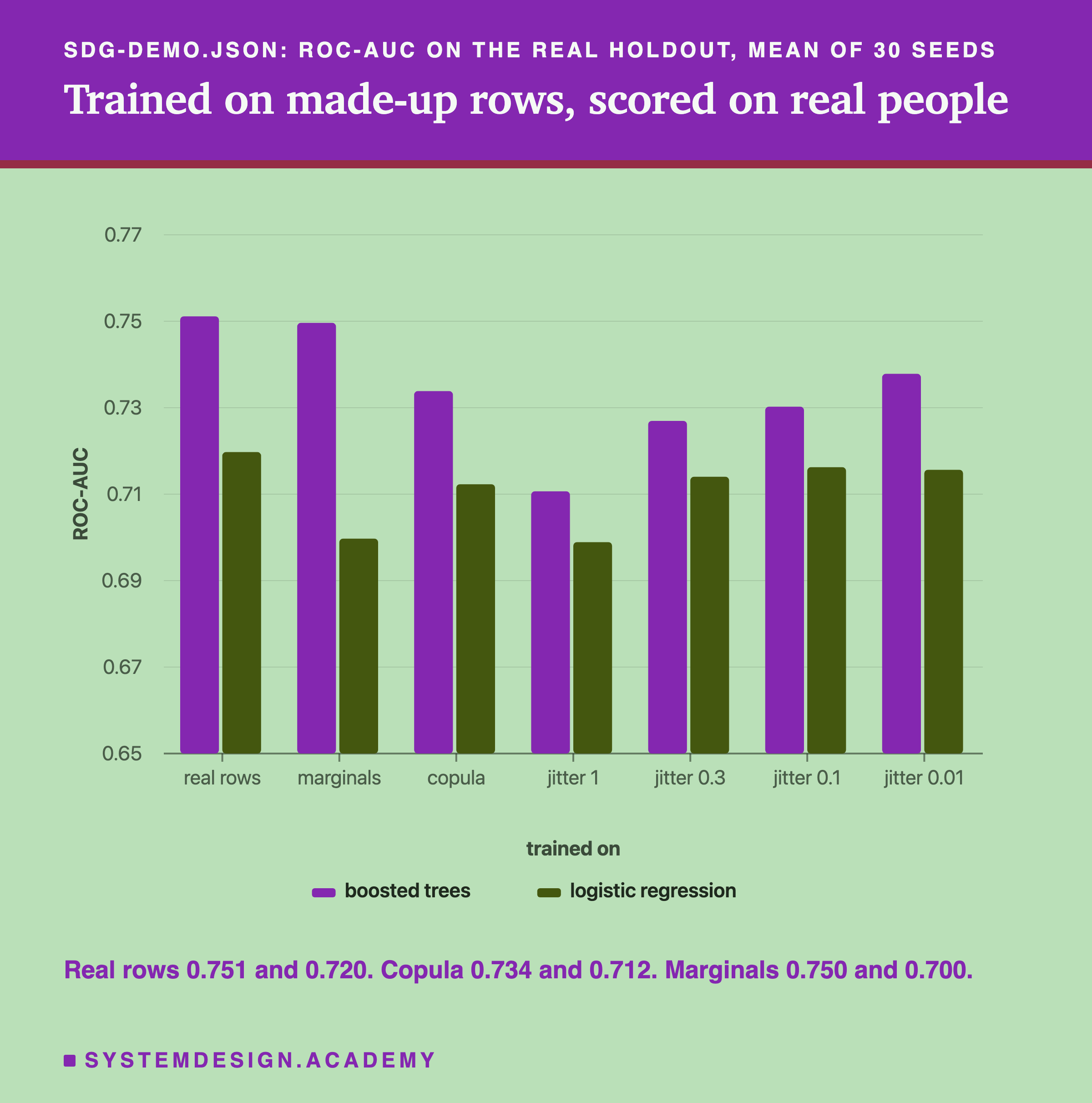
The axis starts at 0.65, so the gaps look bigger than they are. Trained on real rows, boosted trees scored 0.751 and logistic regression 0.720. Trained on copula rows, they scored 0.734 and 0.712. So the made-up rows taught both models most of what the real rows did, but not all of it. For boosted trees, the cost of going synthetic was 0.017 on average.

The jitter rows tell a story too. With the most noise, h = 1, boosted trees fell to 0.711. As the noise shrank, the score rose: 0.727, 0.730, then 0.738 at h = 0.01. Less noise means rows closer to real people, and closer rows teach more. Even the near copies at h = 0.01 stayed below the real rows. One possible reason, checked after the results: jitter picks real rows at random with repeats, so it used only 63.1 percent of the different training rows. The rest were never picked.

The spread across seeds matters as much as the means. With real rows, boosted trees ran from 0.727 on the worst seed to 0.771 on the best. With copula rows, from 0.701 to 0.766. Which 3,000 people land in training moves the score almost as much as the generator does.

Now the vanity score. For each generator, I also took the boosted model trained on its rows and scored it on a fresh batch of rows from the same generator. This is TSTS, train on synthetic and test on synthetic. It is the teacher marking students on her own practice sheet.

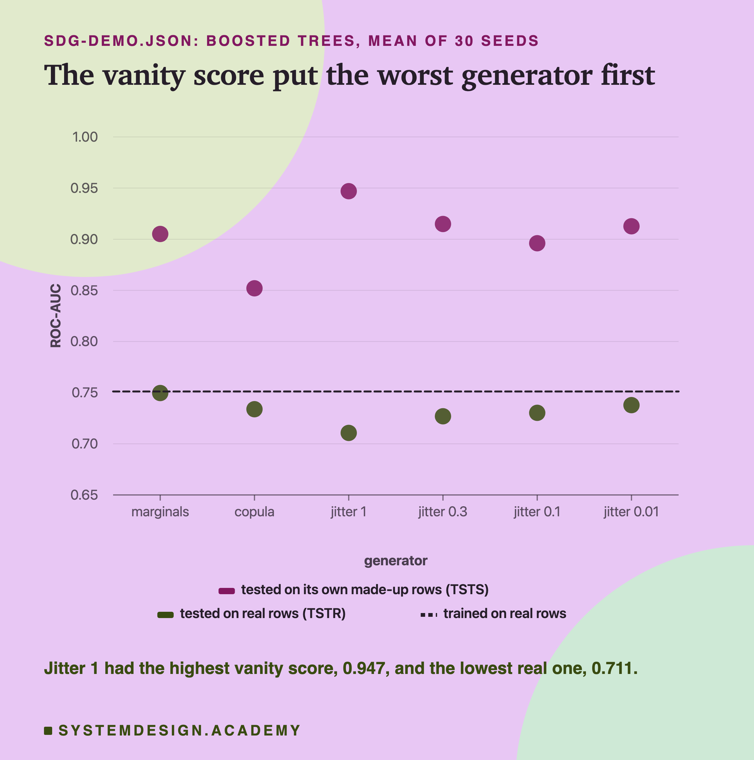
Every vanity score was far above every real one. They ran from 0.852 for the copula to 0.947 for jitter with h = 1. The model trained on real rows and tested on real rows scored 0.751. So a team that only looked at the vanity score would believe its made-up data trains a better model than real data does.

Worse, the vanity score picked the wrong winner. Jitter with h = 1 had the highest vanity score, 0.947, and the lowest real score, 0.711. One possible reason, a guess I did not test: its heavy noise blurs real people's patterns. A model can then learn to tell its own noisy payers and defaulters apart without learning much about real ones.

The ranking was not simply reversed, and I do not want to claim more than the numbers show. Marginals came fourth by vanity score and first on real people. The safe reading is that the vanity score does not tell you which generator to use. Only the score on real people does.

Here is the result I did not expect. The marginals generator throws away every link between columns, yet boosted trees trained on it scored 0.750, almost exactly the 0.751 of real rows. The copula, which keeps those links, scored 0.734.

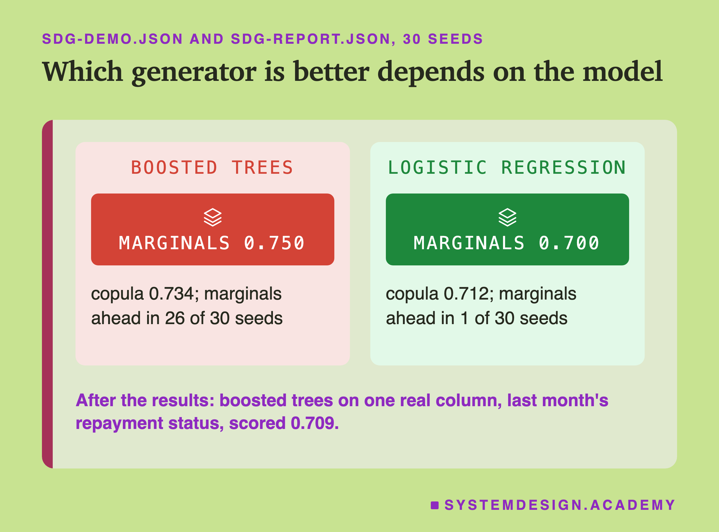
For logistic regression it was the other way round: marginals 0.700, copula 0.712. After the results, I counted seed by seed. Marginals beat the copula in 26 of 30 seeds for boosted trees, and in only 1 of 30 for logistic regression. Marginals' boosted score beat the real rows' score in 14 of 30 seeds, so the two cannot be told apart from seed-to-seed luck.

One possible reason, which I checked after the results: in this data, much of the signal sits in single columns. Boosted trees trained on just one real column, last month's repayment status, scored 0.709. Marginals keep each column's values for payers and defaulters exactly, so a model that mostly reads columns one at a time loses little. Logistic regression adds the columns' evidence together. When six correlated bill columns become six independent ones, it seems to count the same evidence several times. That is a guess, not something I measured.

The lesson is practical. "Is this synthetic data good?" has no answer on its own. Test it with the model you will really train on it.

Fidelity is how closely the made-up rows match the real ones. Utility is how well a model trained on them does on real people, which is what TSTR measures. The simplest check compares columns one at a time, and both of my first two generators pass it perfectly, by construction: they only use real values. So I compared pairs of columns instead. For each of the 253 pairs among 23 columns, I measured the rank correlation: how strongly the two columns rise and fall together, from -1 to 1.

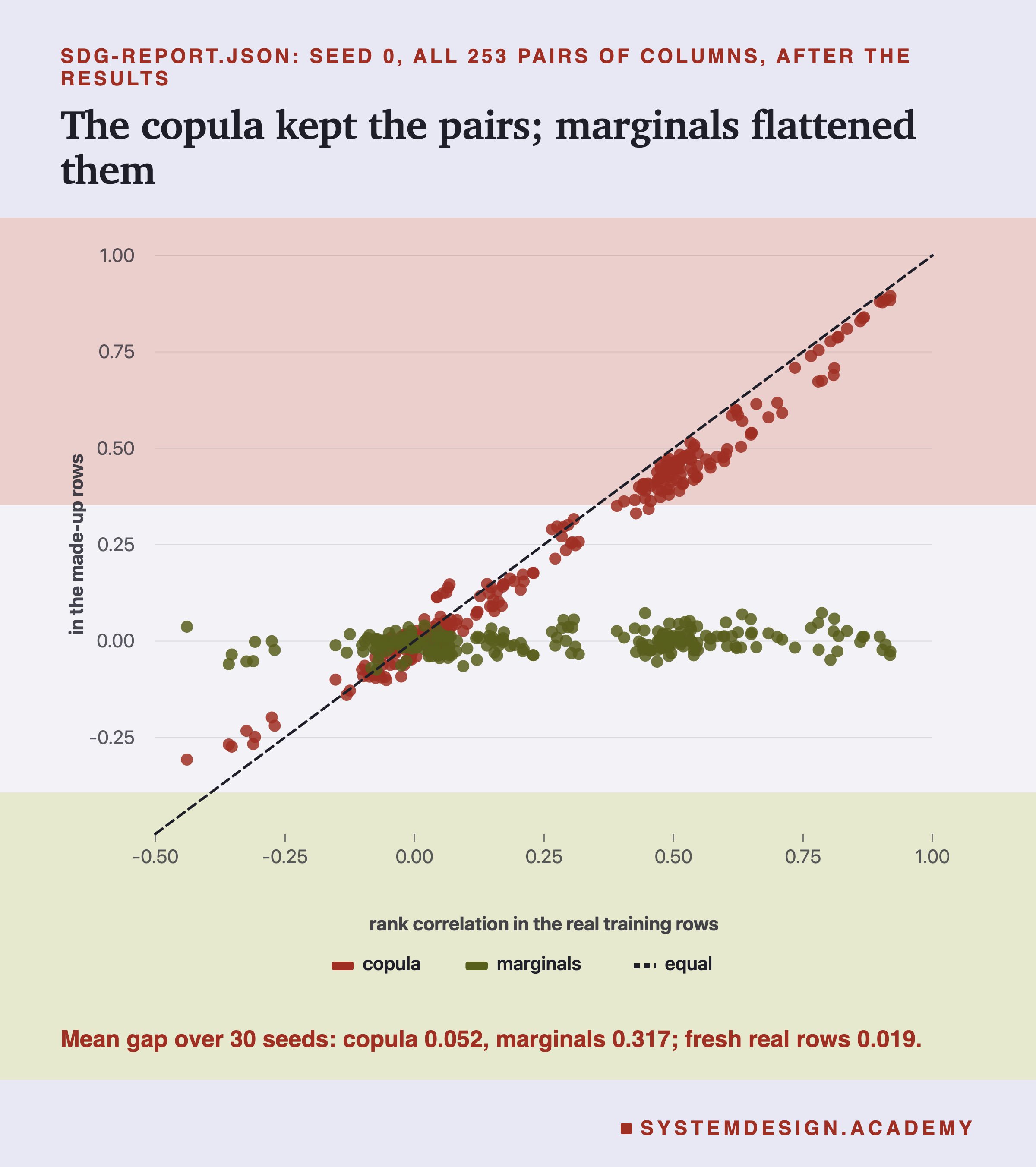
Each dot is one pair of columns on seed 0. Its position across is the pair's correlation in the real rows, and its height is the same pair in the made-up rows. A perfect generator puts every dot on the dashed line. The copula's dots follow the line closely. The marginals' dots lie flat near zero, because each column was drawn on its own. That flat band was certain before the run, and I say so plainly. What the run adds is the size of the copula's gap.

Over 30 seeds, the average gap was 0.052 for the copula and 0.317 for marginals. As a yardstick, the gap between two sets of fresh real people, the training rows and the holdout, was 0.019, the gap that sampling alone gives.

Now put this beside the last slide. Marginals had by far the worst fidelity and, for boosted trees, the best real score. High fidelity and high usefulness are not the same thing, and a fidelity report alone cannot tell you whether a model will work.

The jitter rows show the opposite danger. At h = 0.01 the gap was 0.014, smaller than the 0.019 between two sets of real people. Made-up rows that match the training rows better than fresh real data does are not a triumph. They are a warning that the rows were copied.

That brings us to privacy. The usual first check is distance to closest record, DCR. For each made-up row, find the nearest real training row and measure how far away it is. A row sitting right on top of a real person is a near copy.

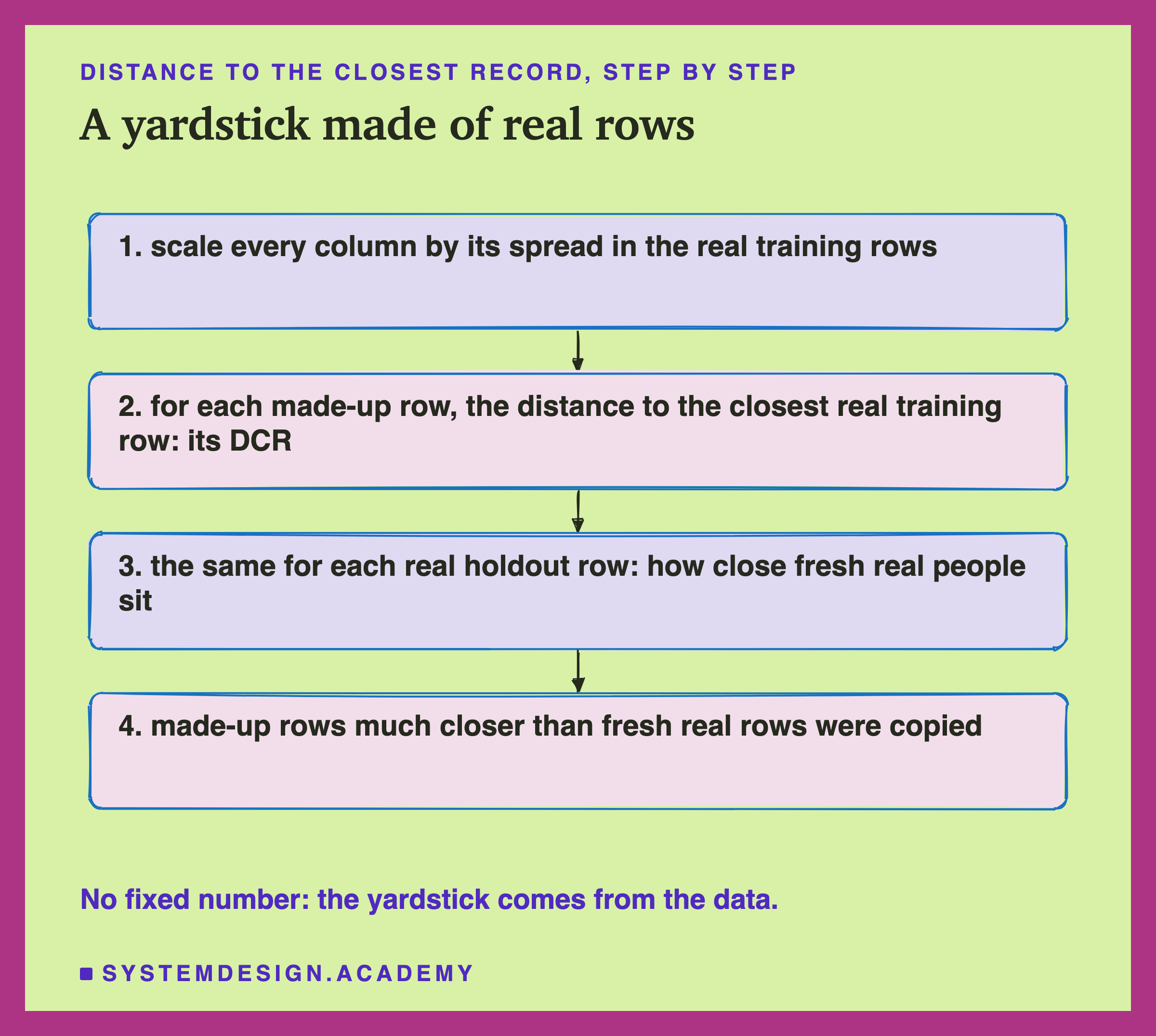
The hard part is deciding what "close" means. A fixed number would be a guess, so I used real people as the yardstick. Each holdout row's distance to its nearest training row shows how close fresh, never-seen people naturally sit to the training people. If made-up rows sit much closer than that, they were copied.

First I scaled every column by its spread in the training rows, so a column measured in dollars does not swamp a column measured in years. Then I used two checks on that yardstick. A percentile is a cut-off in a sorted list. The 5th percentile of the holdout distances is the distance that the closest 5 percent of holdout rows fall below.

The 5th-percentile check counts the made-up rows closer than the closest 5 percent of holdout rows. Fresh real rows would give 5 percent. The nearer-to-training check asks, for each made-up row, whether it sits nearer a training row than any holdout row. If nothing was copied, that should happen about half the time, because the training and holdout people are drawn the same way. This is the same idea as DCROverfittingProtection in the SDMetrics library, with a different distance.

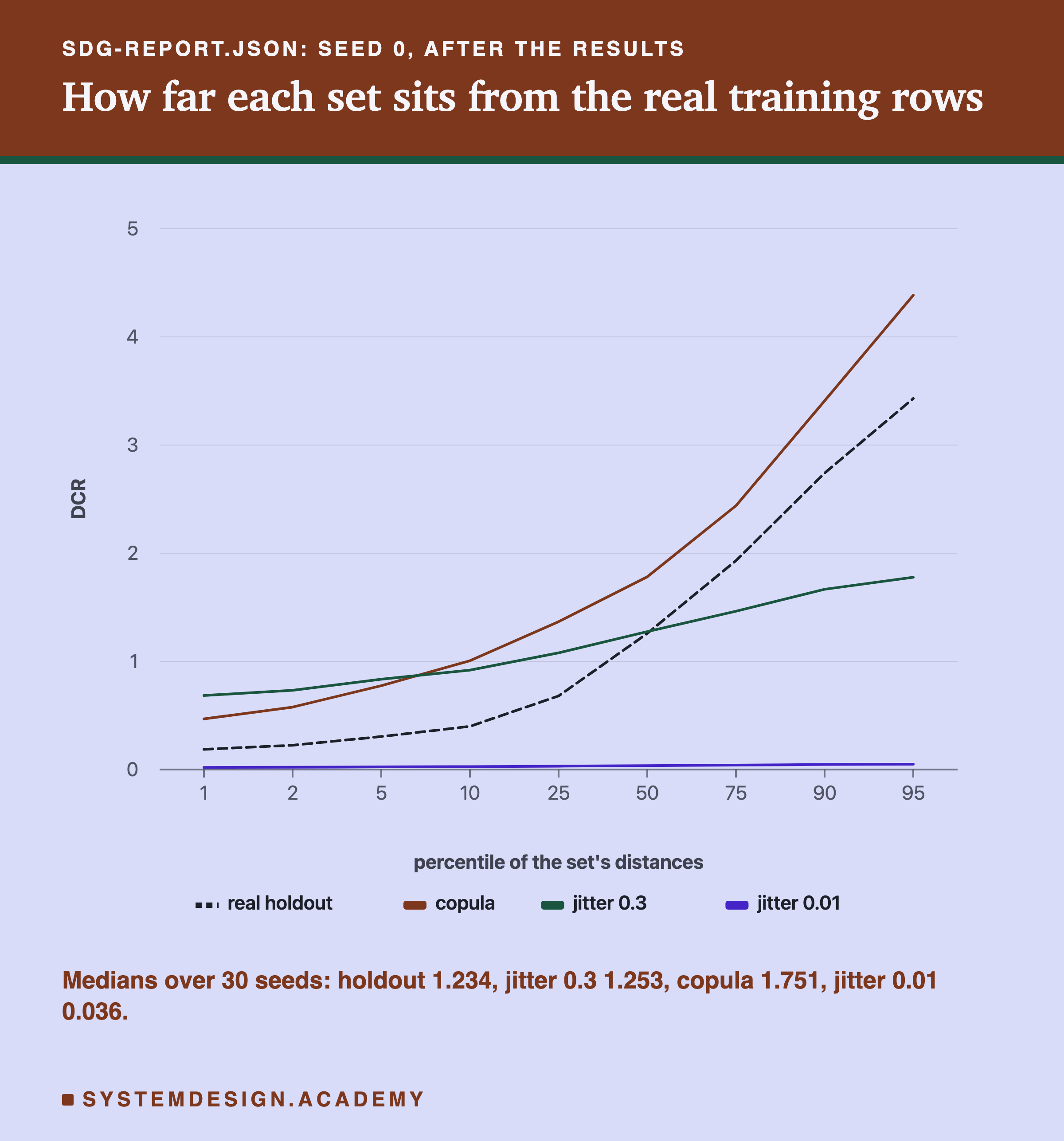
Each line shows one set's distances on seed 0, from its closest rows on the left to its farthest on the right. Jitter at h = 0.01 lies flat along the bottom: every row is almost on top of a real person. The copula sits above the holdout line at most points, so its rows are, if anything, farther from the training people than fresh people are.

Jitter gives me a dial. Turn the noise down and the rows move closer to real people. Here is what the two checks said at each setting.

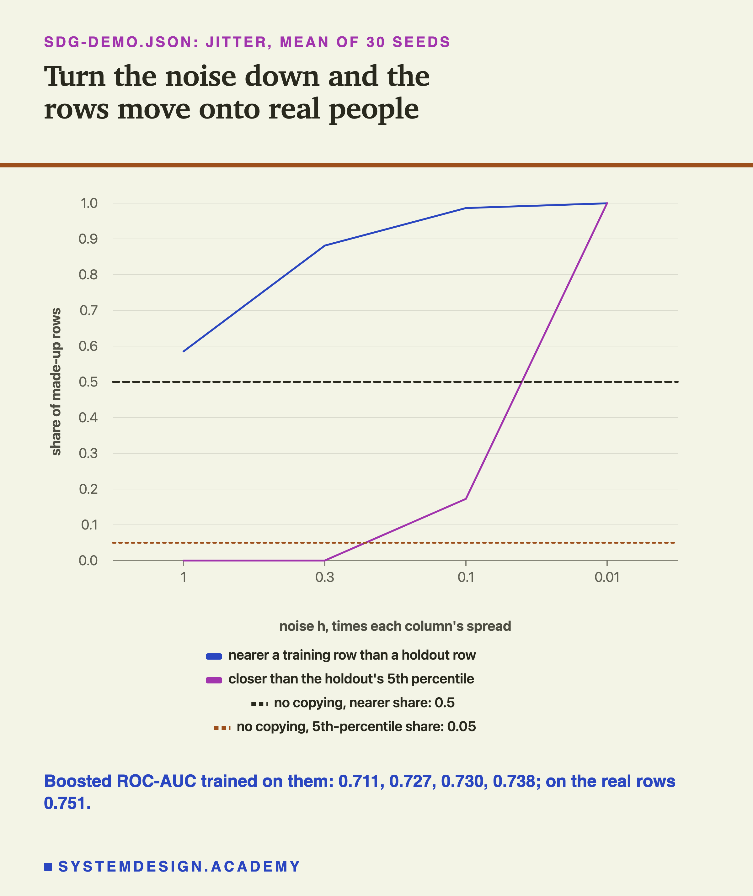
At h = 1 the nearer-to-training share was 58.5 percent, a little above the 50 percent of no copying. At h = 0.3 it jumped to 88.1 percent, at 0.1 to 98.6 percent, and at 0.01 to 99.9 percent. The 5th-percentile check stayed at 0.0 percent for h = 1 and h = 0.3, then read 17.3 percent at 0.1 and 100.0 percent at 0.01.

Meanwhile the real score climbed as the noise fell, from 0.711 to 0.738. Along this one dial, closer rows were more useful and less private. That is not a rule across generators. Marginals sat farthest from real people, a median distance of 2.917, yet were the most useful for boosted trees, 0.750.

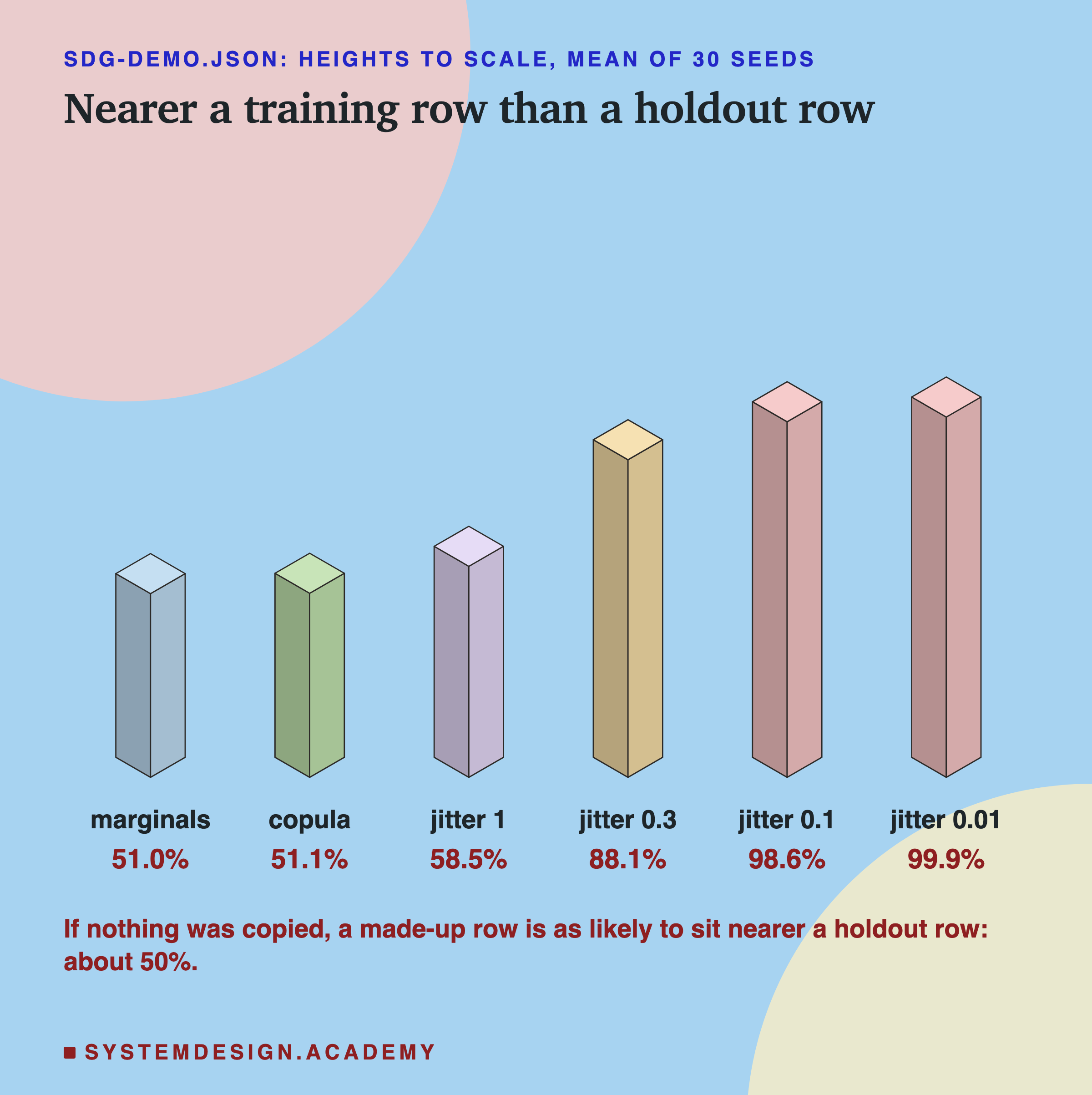
The blocks show the nearer-to-training share for all six generators. Marginals and the copula sat at 51.0 and 51.1 percent, no different from fresh real people. Seed by seed they ran from 48.4 to 54.1 percent and from 48.0 to 54.7 percent. Every jitter setting sat above that, and the three smallest settings far above it.

Put the two checks side by side for jitter at h = 0.3 and the problem is plain.

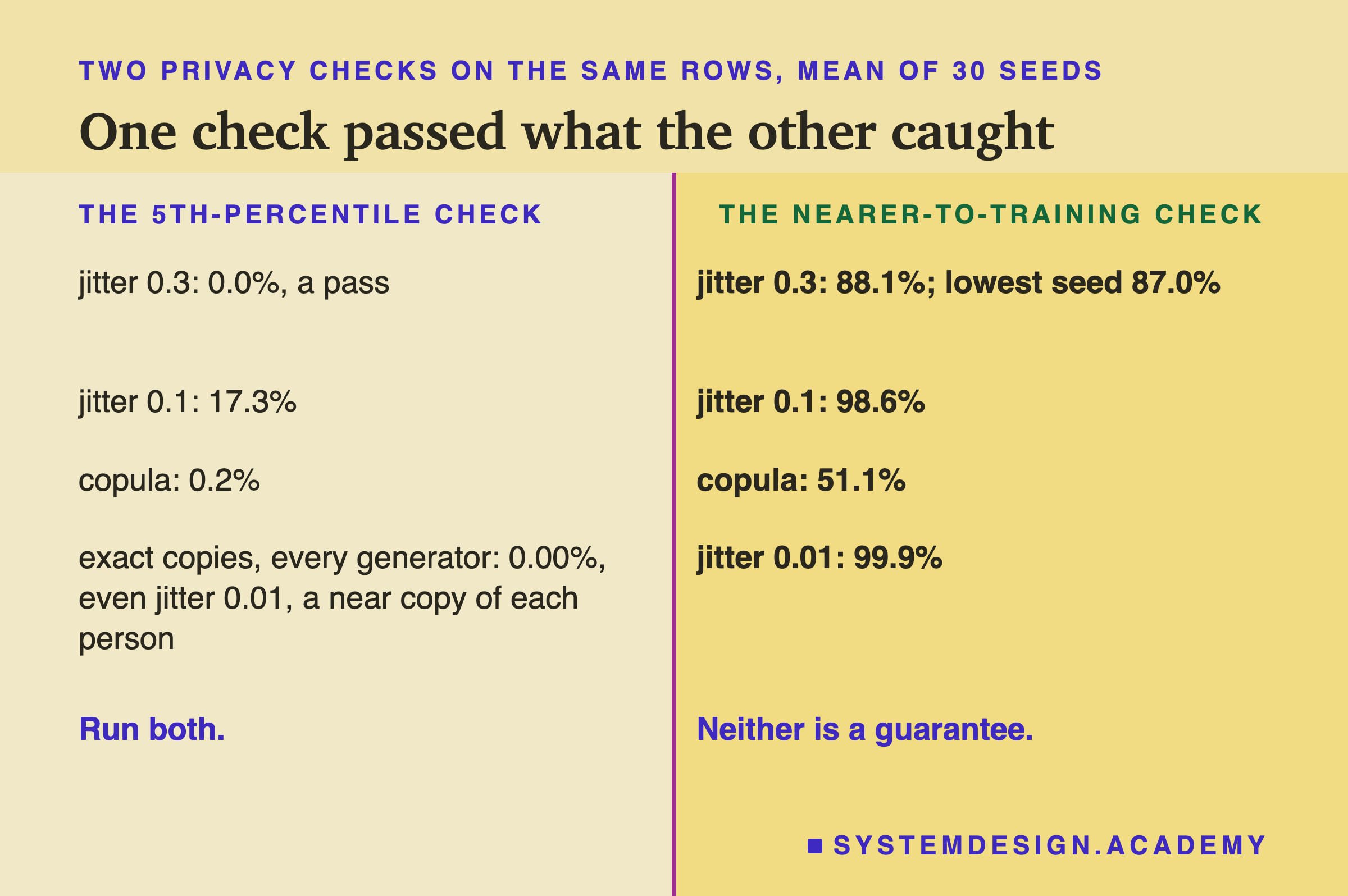
The 5th-percentile check gave jitter 0.3 a clean pass: 0.0 percent of its rows were closer than the closest fresh real people. The nearer-to-training check found 88.1 percent of its rows nearer a training person than any holdout person, and never fewer than 87.0 percent on any seed. Each made-up row sat near the person it was made from, just not as near as some real look-alikes sit to each other. One check looks at the closest few rows; the other looks at every row.

The simplest check of all, exact copies, saw nothing anywhere. No generator made a single row equal to a training row in all 23 columns. That includes jitter at h = 0.01, which is a near copy of every person. Tiny noise is enough to defeat an exact-copy check. Meanwhile 0.04 percent of real holdout rows did equal a training row, because the table holds 56 rows that repeat another row exactly.

A note on how I counted that. My first version counted a copy as a distance of exactly zero. scikit-learn's nearest-neighbour search gave one exact copy a distance of 0.000000146 instead, so I now compare the raw values. Only the holdout's copy counts changed. Also, 158 made-up rows, over all seeds and generators, sat exactly as close to a holdout row as to a training row. Identical rows sit on both sides of the split. I count those as not nearer.

So should a team run both checks and ship? No. The checks can catch a generator that copies. They cannot prove that one does not leak.

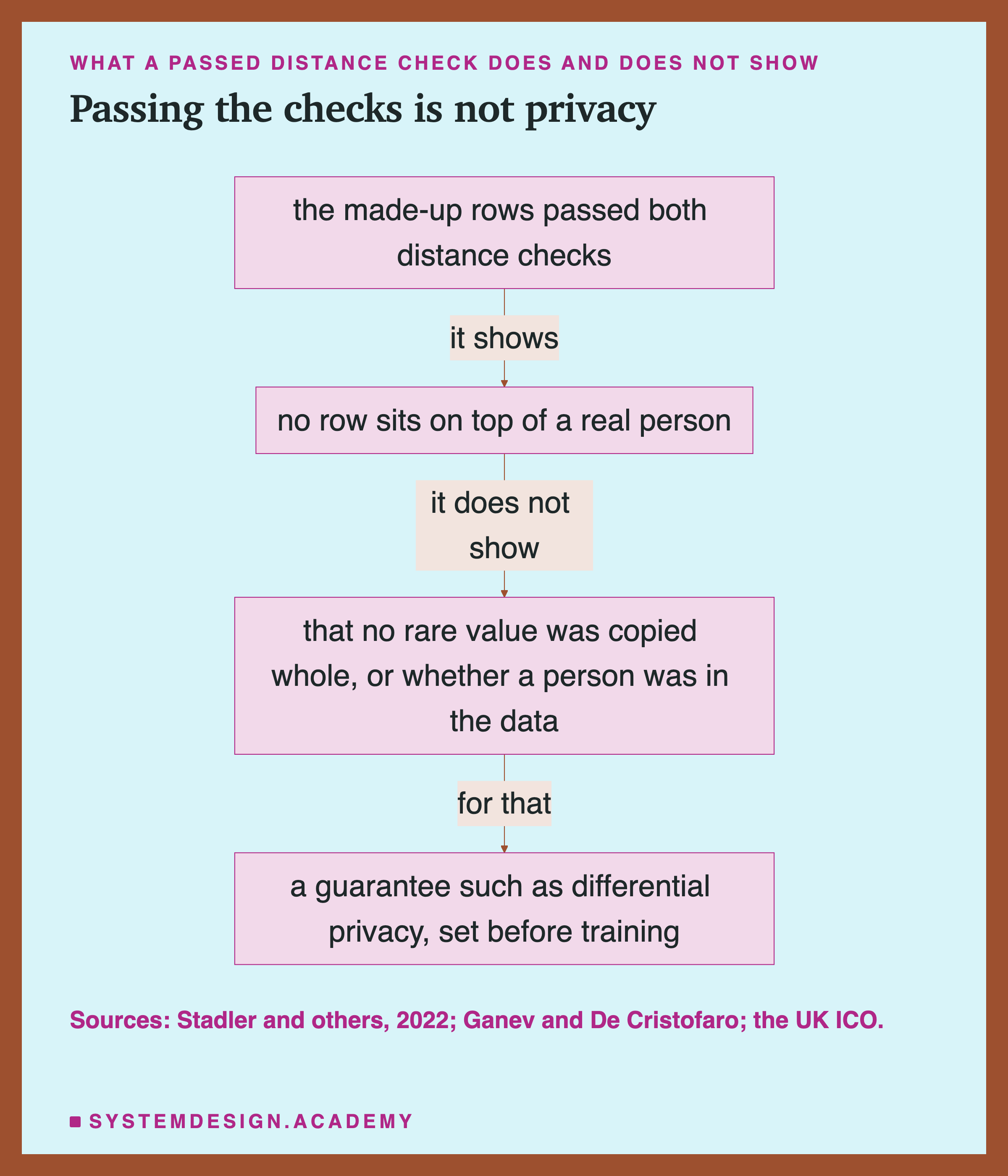
Three published findings say so. In 2022, Stadler, Oprisanu and Troncoso tested many generators and found that "synthetic data either does not prevent inference attacks or does not retain data utility". Ganev and De Cristofaro built attacks that work on synthetic data that passes similarity checks, giving "counter-examples where severe privacy violations occur even if the privacy tests pass". And the UK's data protection regulator, the ICO, asks "Is synthetic data anonymous?" and answers "This depends on whether the personal information on which you model the synthetic data can be inferred from the synthetic data itself."

My own generators show one way this happens. Every value in a marginals or copula row is a value some real person had. If one person has an unusual credit limit or a huge bill, that exact number can turn up in the made-up rows. A distance check looks at whole rows, so it will not notice.

Two kinds of attack are worth naming. Membership inference, from Shokri and others in 2017, decides whether a given record was in the training data. In their words, it is to "determine if the record was in the model's training dataset". Just knowing someone was in a table of loan defaulters can harm them. Training data extraction, from Carlini and others in 2021, goes further and recovers the training examples themselves.

The real defence is a guarantee chosen before training, such as differential privacy, with an epsilon agreed with privacy specialists and legal. The guarantee must cover the whole pipeline, including how each column's values are learned. My copula copies raw values back out, so protecting only its correlation step would still leak those values. Treat any sharing of synthetic data made from people as a legal decision, not a technical one.

The last part of the lab asks the question behind the title. When real rows are few, do made-up rows help? I took only the first 200 training rows. Then I trained each model three ways. First on those 200 real rows; then on those 200 plus 3,000 copula rows made from them; last on the 3,000 copula rows alone. All were scored on the same 3,000 real holdout people.

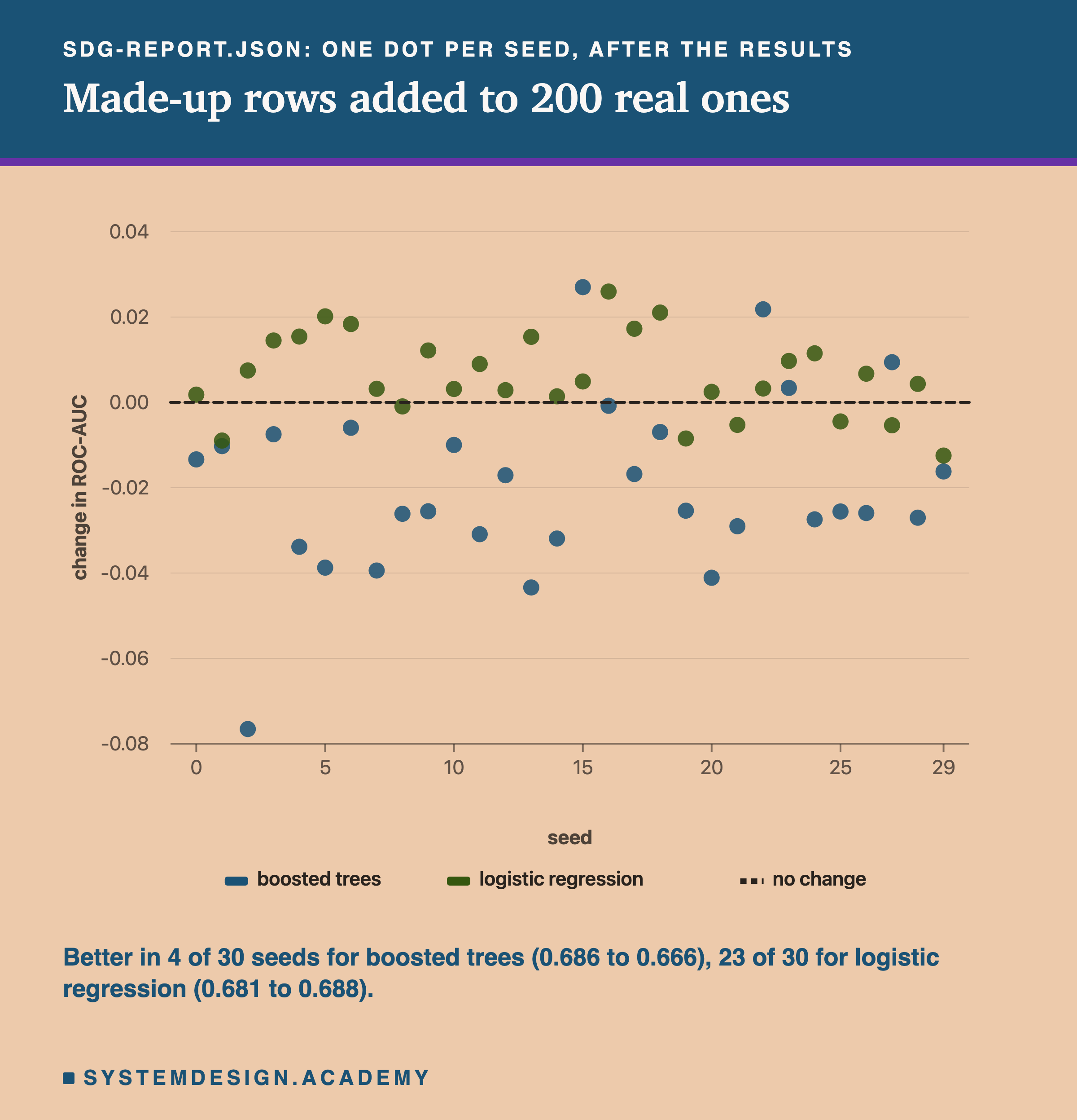
For logistic regression, adding the copula rows helped a little: 0.681 alone, 0.688 with them, better in 23 of 30 seeds. The 3,000 copula rows alone scored 0.687. For boosted trees it hurt: 0.686 alone, 0.666 with them, better in only 4 of 30 seeds, and as much as 0.077 worse on one seed. The copula rows alone scored 0.668.

One possible reason, and it is a guess: the copula smooths the 200 people into a gentle cloud. A simple straight-line model may gain from that steadier picture. Trees can cut the data into small boxes, so they may learn the copula's own smooth shapes, which real people do not have.

Two things are clear. A generator made from 200 people knows only what those 200 people know, so neither model came near the 0.751 and 0.720 that 3,000 real rows gave. And whether made-up rows help again depends on the model. So "fake data beats no data" holds only in a narrow sense. Made-up rows let you train something when you have nothing you may use. On average, no made-up set beat real rows anywhere in this lab. Seed by seed, marginals beat them in 14 of 30 seeds and the copula in 3, and the playground shows both ahead on seed 0.

Synthetic data fails quietly, because each row looks fine until the model does not.

Mode collapse. A GAN can learn to make only a few kinds of row. Each looks real, but the variety is gone. Only comparing the whole spread of the made-up rows with the real ones catches it.

Copying the gaps. A generator learns what is in the data, including what is missing. If a group of people is barely present in the real rows, it will be barely present in the made-up rows too. Check the made-up set for fairness the same way you would check the real one.

Model collapse. This is about training a generator on another generator's output, again and again.

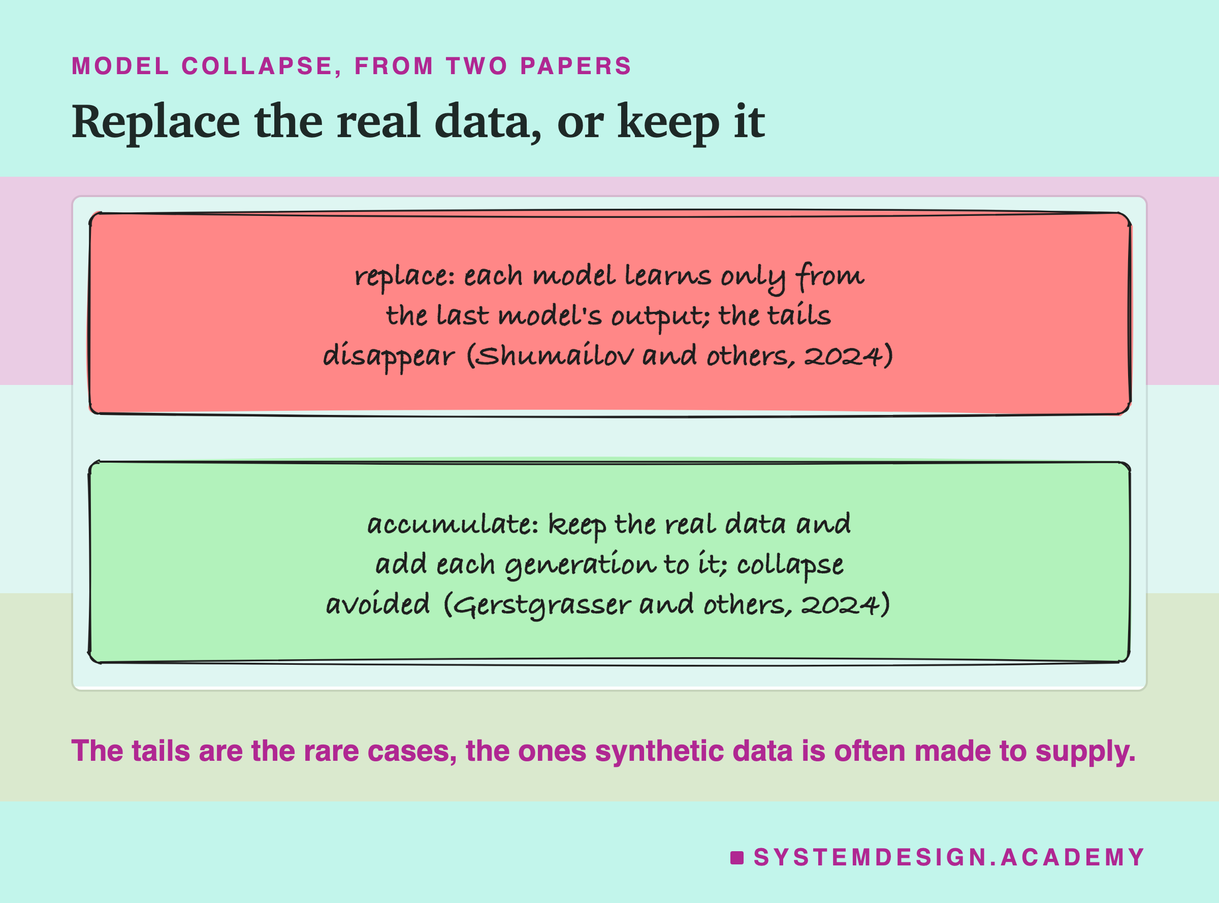
Shumailov and others reported in Nature in 2024 that training on model-made content, without care, causes defects "in which tails of the original content distribution disappear". The tails are the rare cases, the very ones synthetic data is often made to supply. Gerstgrasser and others found the way out in the same year: "accumulating the successive generations of synthetic data alongside the original real data avoids model collapse". So keep the real data in every training mix, and do not replace it.

Synthetic data is in real use. Here is what each organisation says itself, and no more.

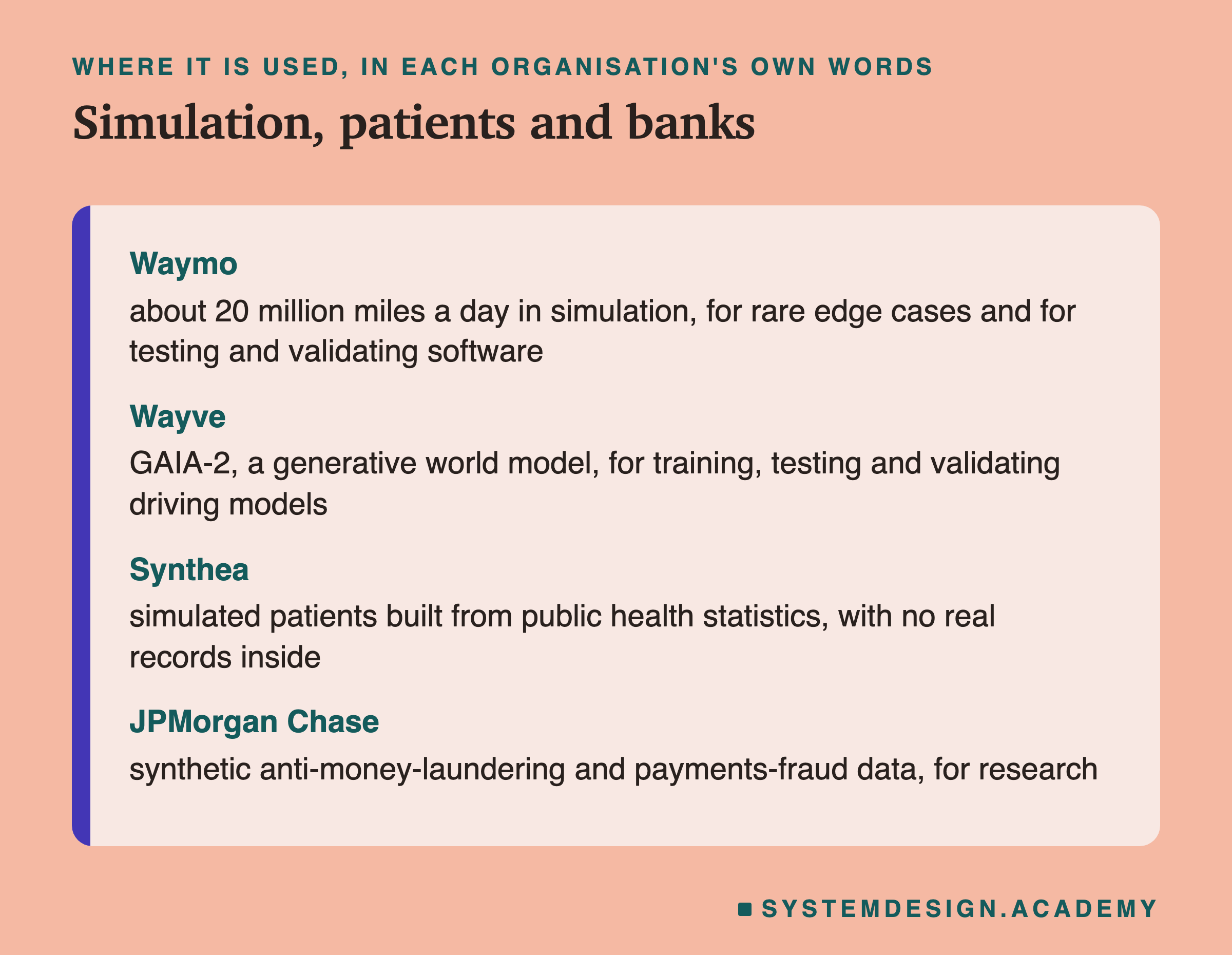
Driving. Waymo wrote in 2020 that "in simulation, we drive around 20 million miles a day". It uses simulation to "prepare for rare edge cases, explore new ideas, validate and test new software". Wayve describes its GAIA-2 world model as being for "training, testing, and validating" driving models. The gap between a simulated road and a real one has a name, the reality gap, which is why both still drive real miles. The earlier version of this lesson said simulated miles outnumber real miles "in their training data". Neither company says that, so I cut it.

Health. Synthea is an open-source tool that makes synthetic patients. It does not learn from real patient records at all. It simulates patients from published health statistics, so there is no real person inside to leak. NHS England has also piloted artificial data for analysts. The earlier lesson said differential privacy is "standard" here. It is not; NHSX wrote that it was still researching it.

Banking. JPMorgan Chase's AI research team publishes synthetic data sets, including anti-money-laundering and payments-fraud data, for research use outside the bank.

You do not have to write generators yourself. Here is what the main tools do, from their own documentation.

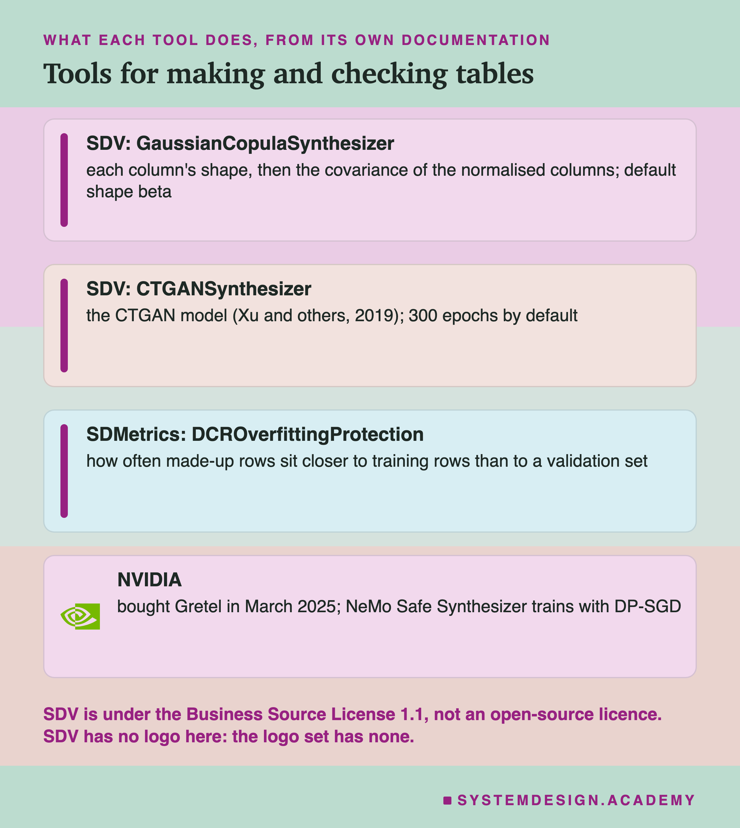
SDV, the Synthetic Data Vault, from the company DataCebo, is the best-known Python library for tables. Its GaussianCopulaSynthesizer learns each column's shape, turns the columns into normal scores and learns how they move together, like my copula. By default it fits each column with a shape called a beta distribution, where mine maps back through the real values. Its CTGANSynthesizer trains a CTGAN, with 300 epochs (passes over the data) by default. Check the licence before you build on it: SDV is under the Business Source License 1.1, not an open-source licence.

SDMetrics, from the same team, scores synthetic data. Its DCROverfittingProtection measures how often made-up rows sit closer to the training rows than to a validation set, which is my nearer-to-training check. It uses a different distance: each number column is scaled by its range, and a category counts 0 if equal and 1 if not.

Gretel was a synthetic data company. NVIDIA bought it in March 2025. NVIDIA's NeMo Safe Synthesizer trains with DP-SGD, the differential privacy method from the GAN slide.

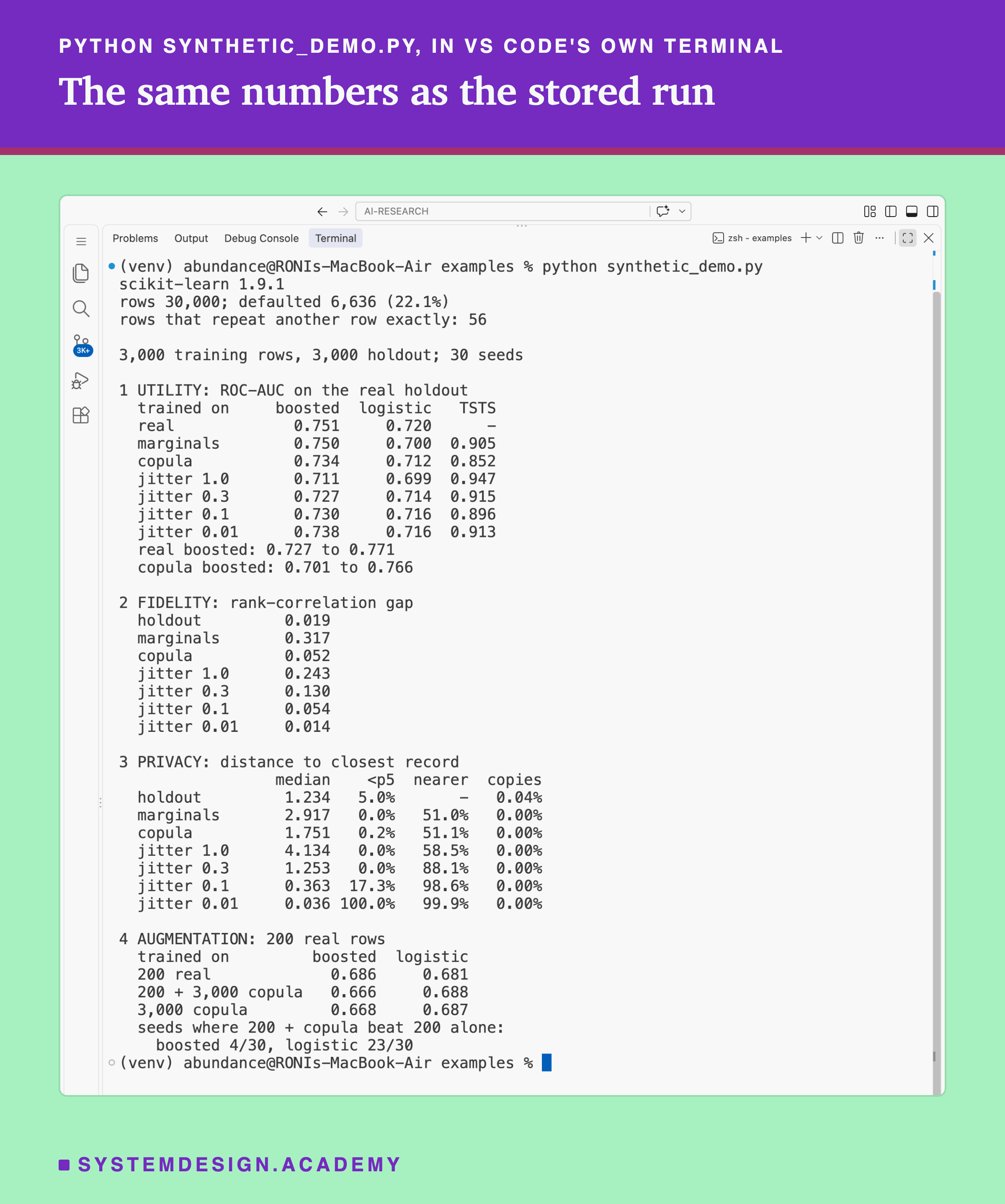
This script is the lab. It downloads the data, then runs all four parts: utility, fidelity, privacy and augmentation. It needs no GPU. On my laptop it ran in well under a minute, and it prints no timings.

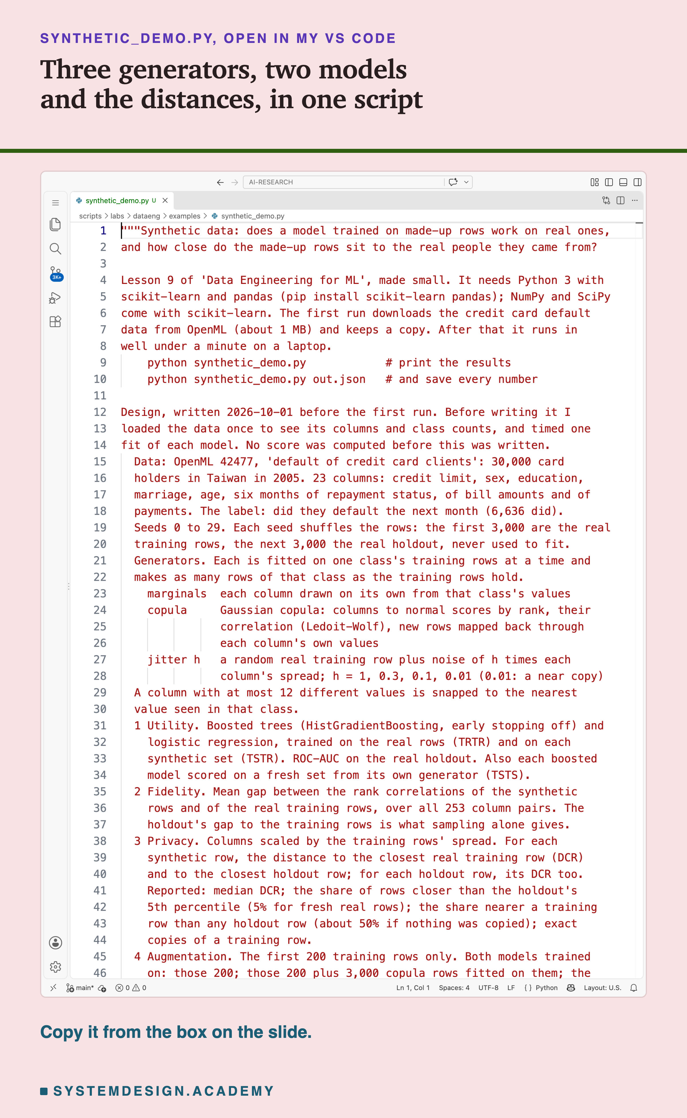
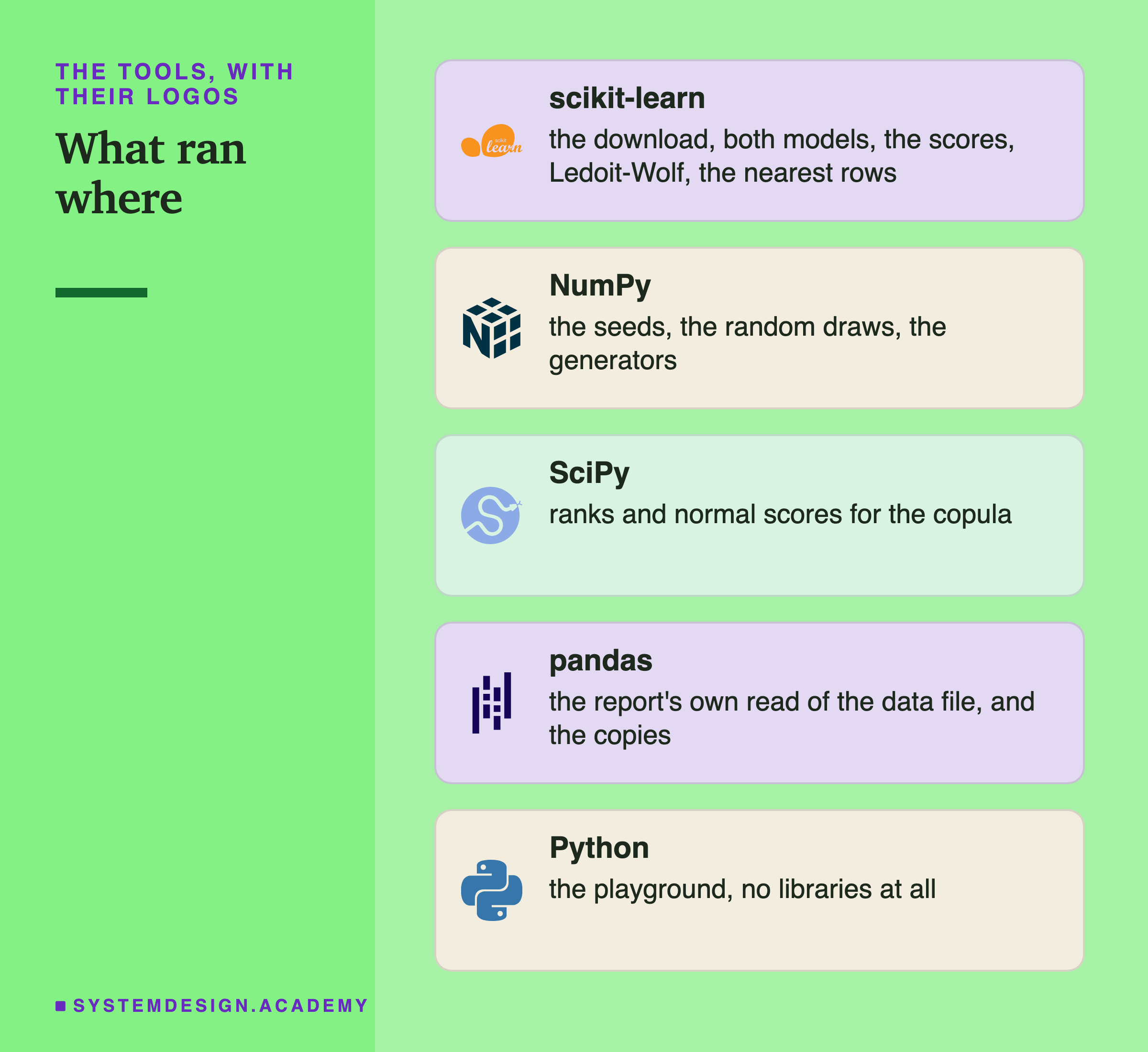
Before you run this lab. You need Python 3 and two libraries: pip install scikit-learn pandas. scikit-learn does the download, the models, the scores and the nearest-row search, and brings NumPy, SciPy and joblib with it. pandas is what scikit-learn uses to read the downloaded table. The first run downloads the data from OpenML (about 1 MB), so it needs an internet connection once. After that, scikit-learn keeps a copy in a folder in your home directory (scikit_learn_data).

I ran it with scikit-learn 1.9.1 on a Mac. These libraries run on Windows and Linux too, but I have not checked the numbers there. Another version of scikit-learn may give slightly different scores, so the first line printed is the version. Give it a file name, python synthetic_demo.py out.json, and it also saves every number. That is how results/sdg-demo.json was made. Two runs gave byte-for-byte the same file.

Two changes came after the first run, and the docstring lists both. First, for speed only: the boosted model is now fitted once per generator, not twice, and the 30 seeds run side by side. The saved file came back byte for byte the same. Second, the exact-copy fix from the checks slide, which changed only the copy counts.

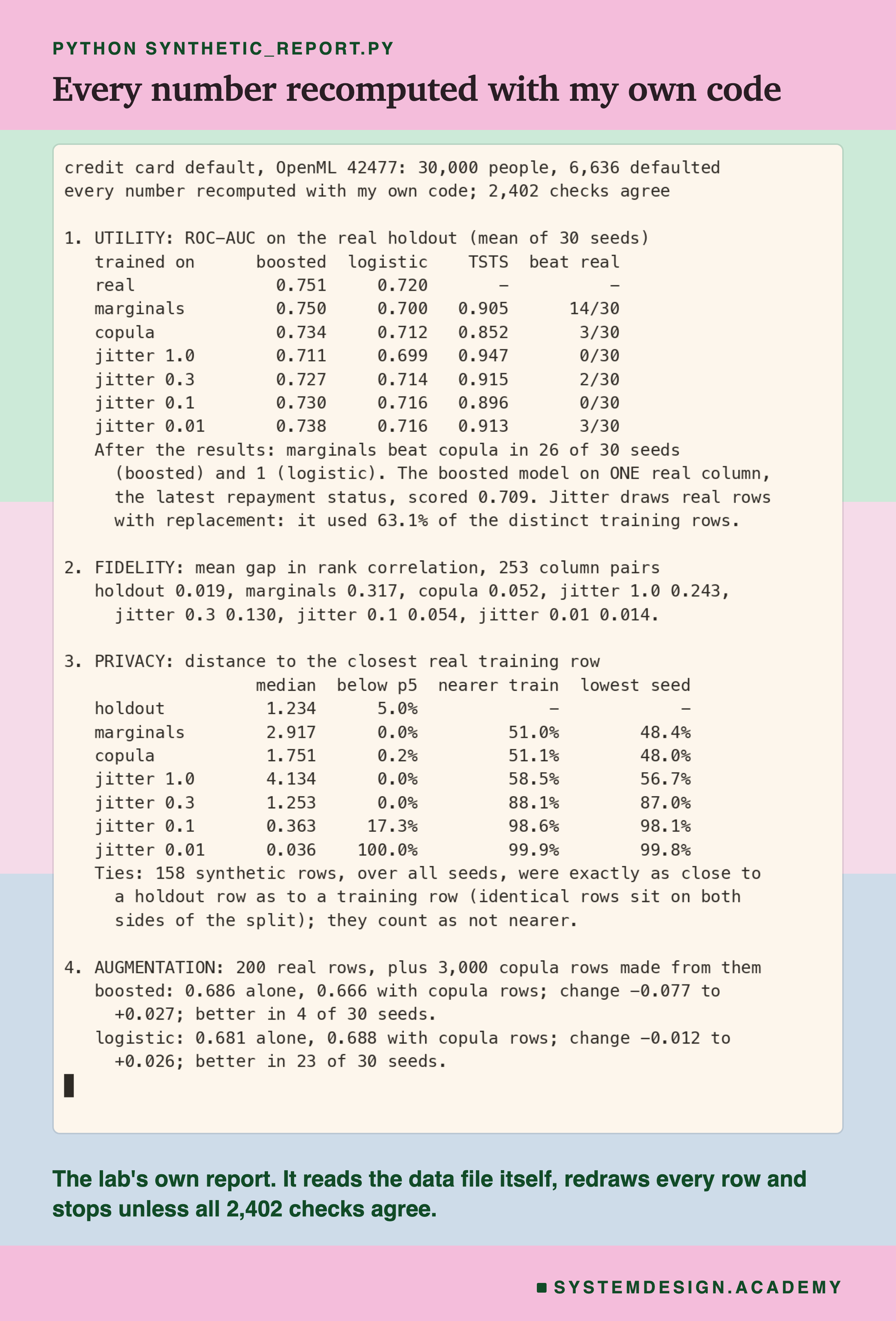
The report lives in scripts/labs/dataeng/synthetic_report.py. It does not trust the demo's code for anything it can redo another way.

It reads the downloaded data file itself. That file has one extra column, a row number, which scikit-learn drops when it loads the data. The report skips that column and checks that the other 23 match the demo's. It redraws every made-up row with its own code, in the same random order, so the rows must come out identical. The copula's covariance step and its random draws use the same NumPy and scikit-learn calls, so that part is not independent. It refits the same models, because the models must be the same.

Then it computes every score with its own code. ROC-AUC comes from ranks, and every distance is worked out by brute force instead of scikit-learn's search. The rank correlations come from pandas, and so do the exact copies, by matching rows.

It covers all 30 seeds, all six generators and both models. Every number must come back within one part in a billion, and 2,402 checks agreed. The two shares that compare distances get one allowance. A row exactly as close to two real rows is a tie, and two codes may round it either way. So the stored share must lie between the counts with ties counted each way.

Its json mode writes results/sdg-report.json, which the figures read. Its demo mode checks the demo's printed run line by line. Its box mode writes the playground on the next slide and checks it.

What came when: the demo's design, in its docstring, came before any run. Five things came after I saw the results, and the report's docstring lists them. They are the seed-by-seed counts, the one-column score and the share of rows jitter used. The other two are the seed 0 correlations and distances, and the augmentation changes seed by seed.

This box holds seed 0's real distance counts for all six generators. It has no model and no data rows. It runs in your browser.

As it is, the box prints the copula on seed 0. 3 of its 3,000 rows sat closer than percentile 5 of the holdout distances: 0.1 percent, against about 5 percent for fresh real rows. 50.5 percent sat nearer a training row. Then set GENERATOR = 'jitter 0.3' and watch the first check pass while the second reads 88.3 percent. Try PCT = 50 too: about half its rows now count as close, which is roughly what fresh people give.

One more thing to notice. On seed 0, boosted trees trained on marginals scored 0.772 and on copula rows 0.766, both above the 0.755 of real rows. Over 30 seeds, neither beat the real rows on average. One seed is one draw.

The data. fetch_openml(data_id=42477) downloads the table once and reads the local copy after that. X holds the 23 columns as numbers, and y is 1 for a person who defaulted and 0 for one who paid. np.unique counts the rows that repeat another row exactly.

make and synth. make is the three generators. For marginals, rng.choice picks each column's values on its own. For the copula, rankdata turns each column into ranks and norm.ppf turns ranks into normal scores. LedoitWolf measures how they move together and multivariate_normal draws new scores. Then np.quantile with method="inverted_cdf" maps each one back to a real value. For jitter, rng.integers picks real rows and rng.normal adds the noise. snap then rounds the columns with few values. runs once per class.

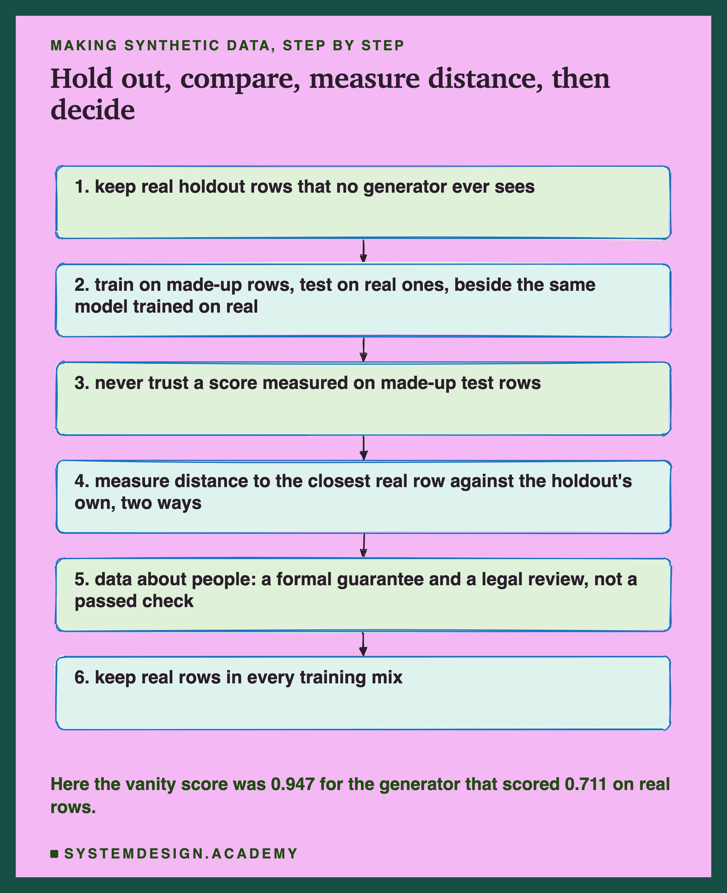
Keep a real holdout. Set aside real rows before anything else, and never let a generator see them. Without them you cannot measure either usefulness or privacy.

Compare TSTR with TRTR. Train the same model on made-up rows and on real rows, and score both on the holdout. Use the model you will really train: here the better generator depended on it.

Never trust a score on made-up test rows. Here the vanity score was 0.947 for the generator that scored 0.711 on real people.

Measure distance two ways. Compare made-up rows with the holdout's own distances, using both the closest few rows and the nearer-to-training share. Here jitter 0.3 passed one and failed the other.

Get a guarantee for data about people. A passed check is not privacy. If the source data is about people, use a method with a formal guarantee, such as differential privacy, and get a legal review before sharing.

Keep real rows in the mix. Add made-up rows to real ones rather than replacing them, and check that adding them helps your model.

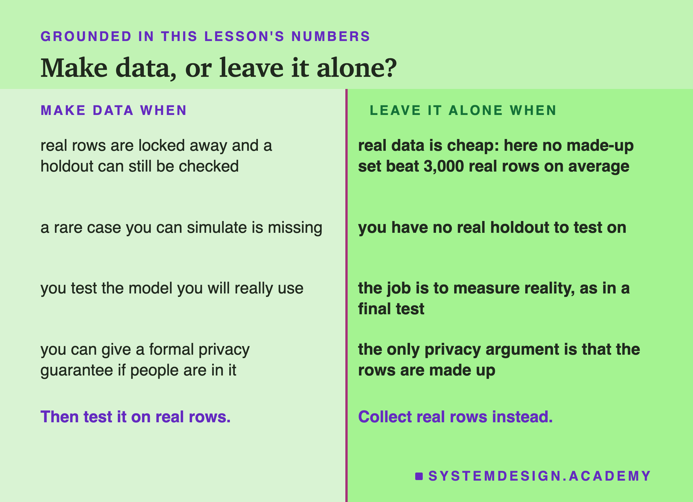
Make data when the real rows are locked away but you can still test on a real holdout. Also when a rare case is missing and you can simulate it from known rules, and when you will test the result with the model you really use. If people are in the source data, share or release it only when you can give a formal privacy guarantee.

Leave it alone when real data is cheap: here no made-up set beat 3,000 real rows on average, and marginals only tied them, 0.750 against 0.751. Also when you have no real holdout to test on, because then you are guessing. Never use made-up rows to measure reality, such as a final test or an audit. And never rely on "the rows are made up" as the privacy argument.

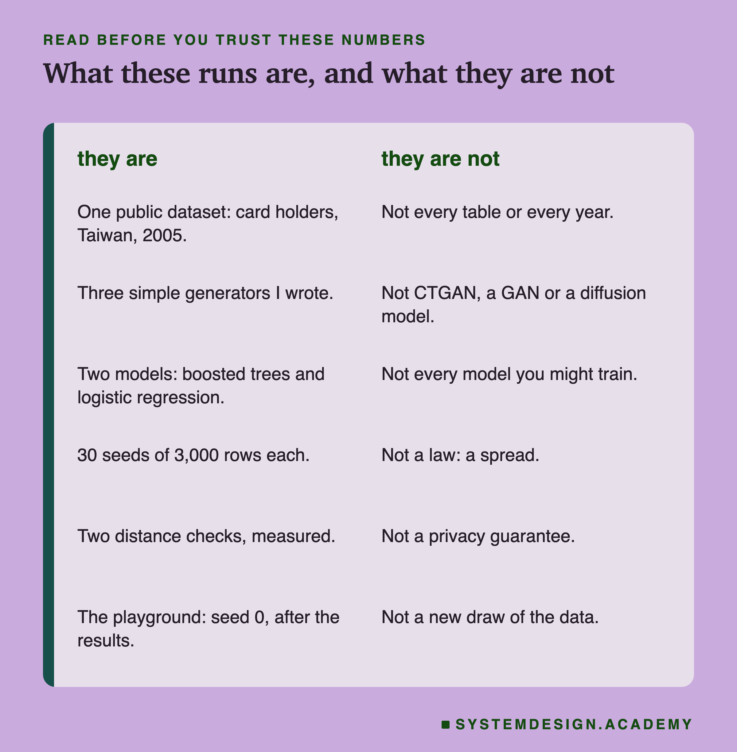
One dataset. Card holders in Taiwan in 2005. On a table where the signal lives in combinations of columns, marginals would probably do much worse than here.

Three simple generators. Not CTGAN, a GAN or a diffusion model. A learned generator may land anywhere on the trade-off; that is exactly why you measure it.

Two models. The better generator flipped between them, so a third model could behave differently again.

Two distance checks. They caught a generator built to copy. Passing them is not a privacy guarantee, as the published attacks show.

What came after the results. The seed-by-seed counts, the one-column score, the share of rows jitter used, the seed 0 figures and the augmentation changes all came after I saw the results.

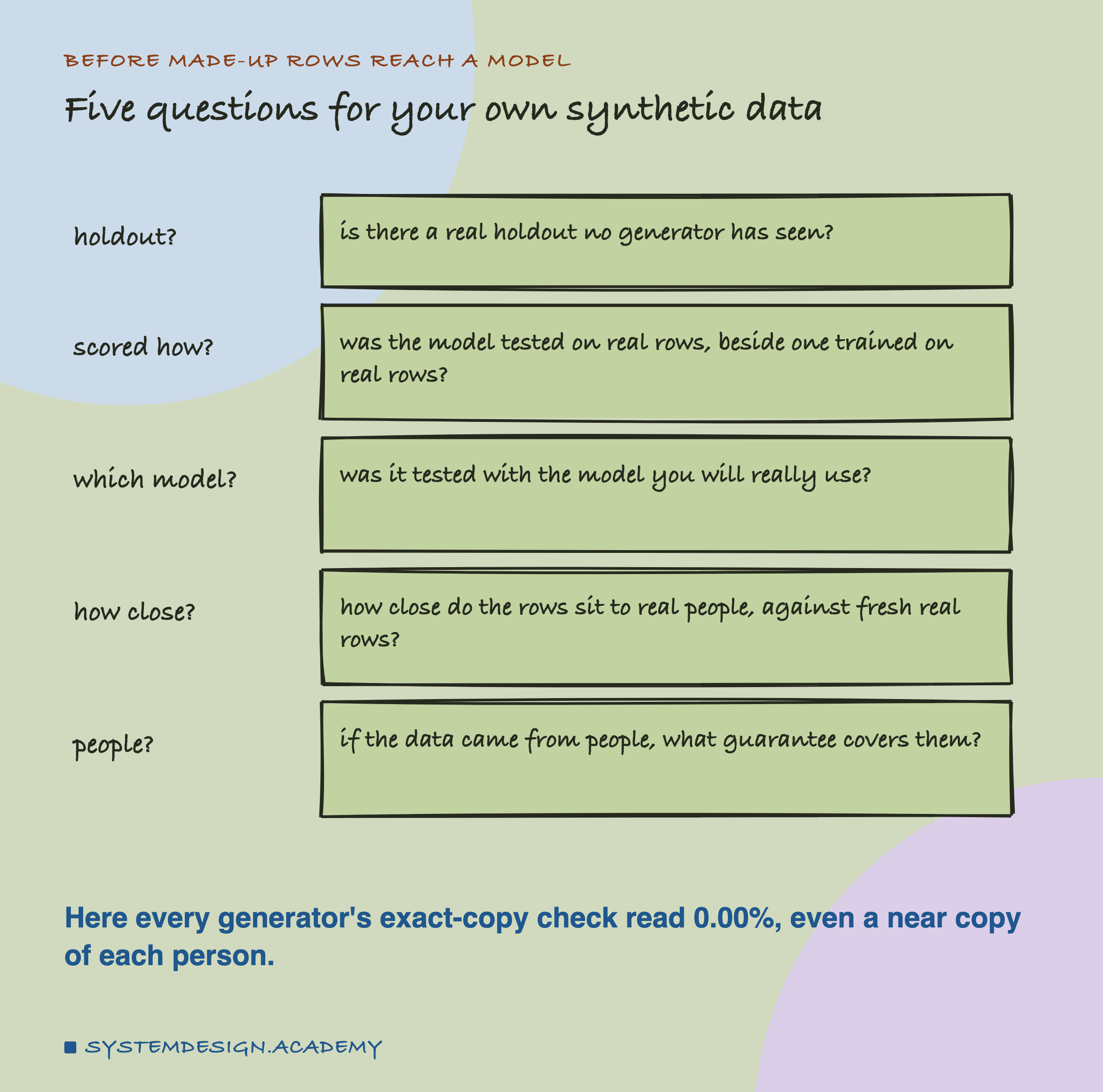
If your team uses synthetic data, ask the first question today: is there a real holdout that no generator has seen? If not, nobody knows whether the made-up rows teach anything true.

Then ask how close the rows sit to real people, measured against fresh real rows, and what protects the people the data came from. Here, an exact-copy check read 0.00 percent even for rows that were near copies of every person.

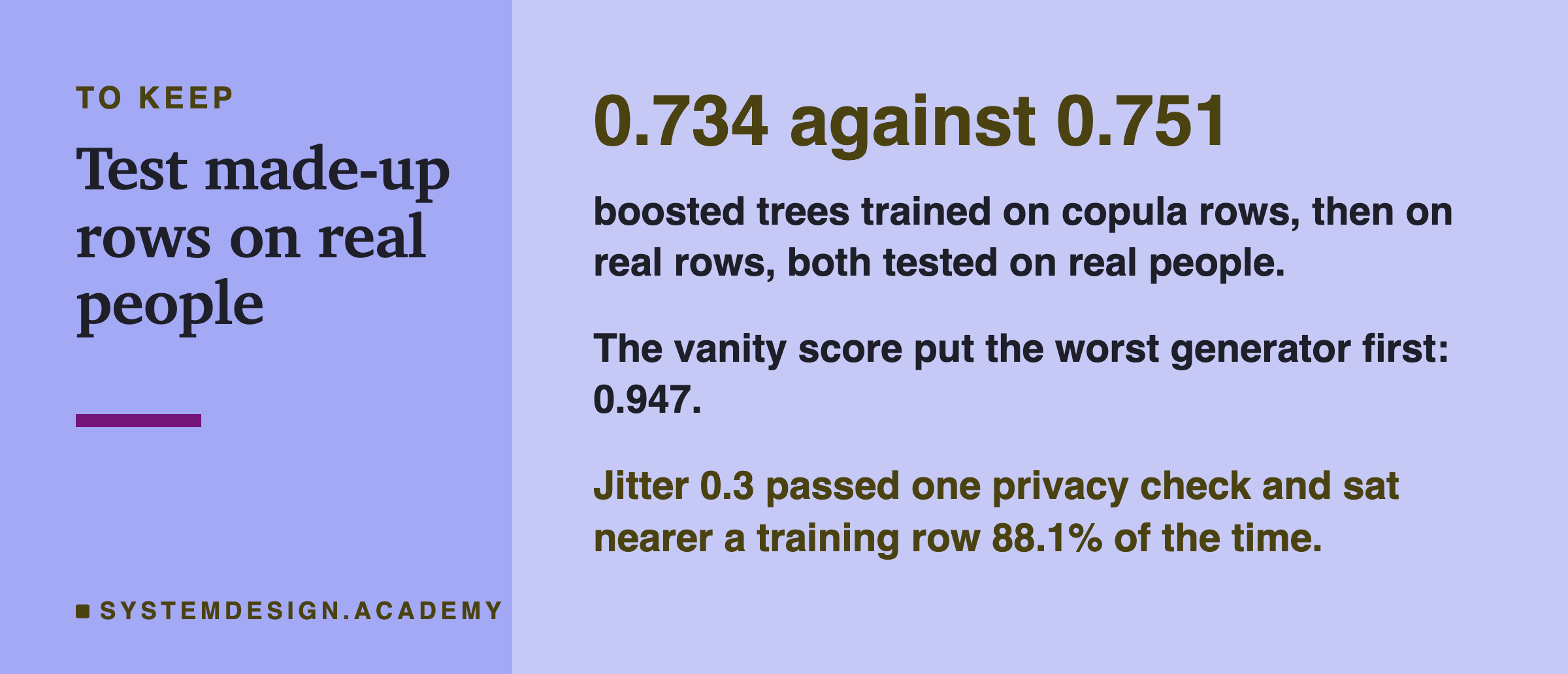
The card keeps the lesson's three numbers. Copula rows taught boosted trees to 0.734 on real people, against 0.751 for real rows. The vanity score put the worst generator first, at 0.947. And jitter at h = 0.3 passed one privacy check while 88.1 percent of its rows sat nearer a training person than a fresh one.

The next lesson in this chapter is about data contracts and schemas: agreeing, in writing, what the data a model depends on must look like.