The New Clerk and the Morning Post
Imagine your first morning at a new office job. The post has arrived: 3,450 letters. Your task is to sort them into two trays, keep and bin. Your manager is busy. She can sit with you for a while and look at 100 letters, and no more.
Which 100 do you show her? If you show her the letters you are already sure about, a bank statement or a pizza flyer, her answers teach you nothing new. If you show her the letters that make you stop and frown, every answer she gives you changes how you sort the next pile.
You also arrive with a few rules of thumb. A letter shouting about free money is usually junk. A letter that uses your boss's first name usually is not. Rules like these sort a lot of letters without asking anyone at all. They are sometimes wrong, and you know it.
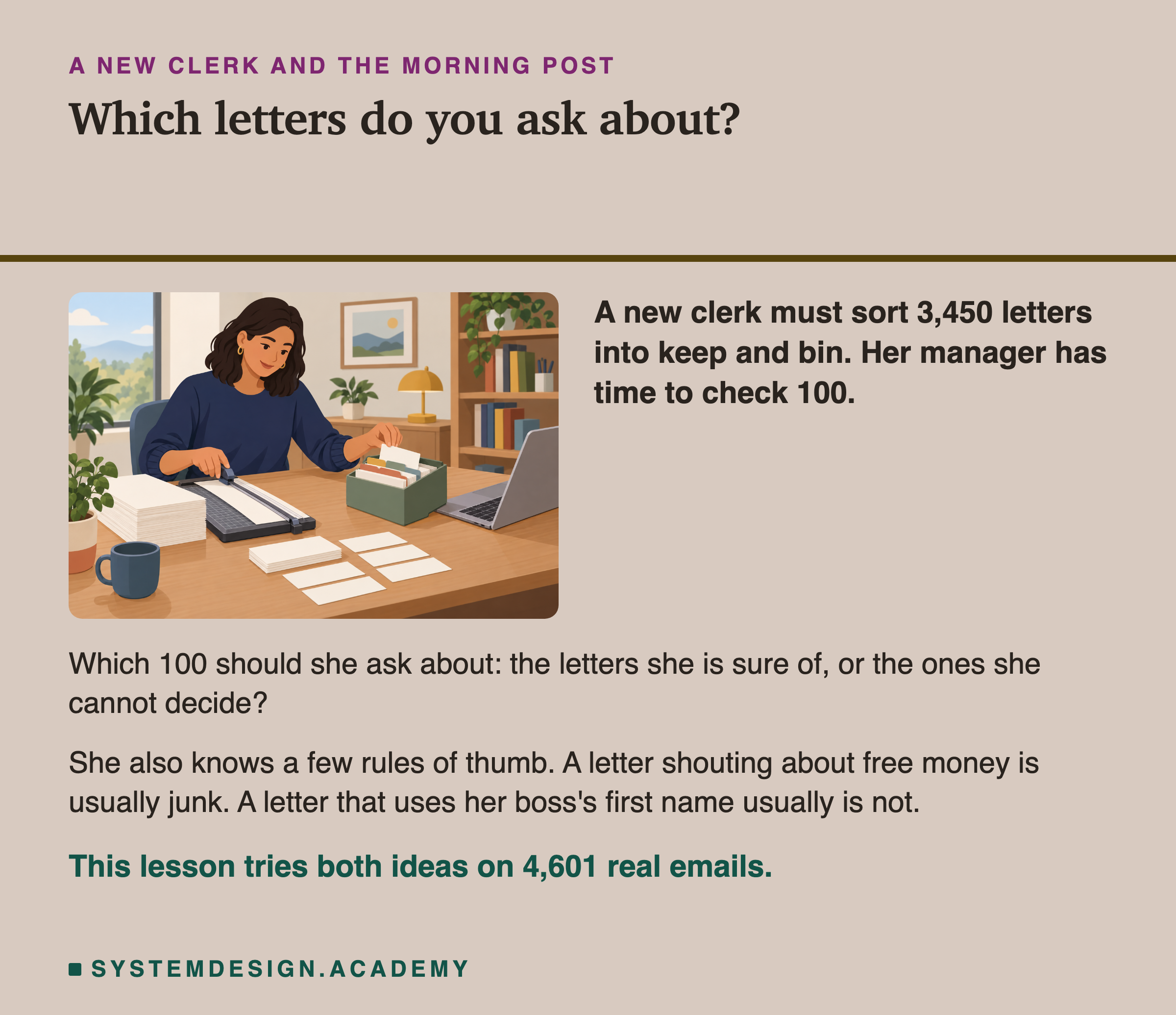
The picture puts the whole lesson on one page. The clerk has far more letters than her manager has time for, so every question she asks has to count. And she already knows things that can sort some letters for free.
A computer that learns from examples has exactly this problem. It needs examples with the right answer attached, and a person has to attach most of those answers. People are slow and cost money, so the answers are usually the most expensive part of the whole project.
In this lesson I take 4,601 real emails, hide their answers, and try four ways of getting them back. I pay for answers picked at random. I pay for the ones the computer is least sure about. I let ten rules of thumb answer for free. Or I pay for all of them. Then I measure how good the computer gets with each one, and I repeat the whole thing 30 times so that luck cannot pick the winner.
Where This Lesson Starts
This is the seventh lesson of the chapter on data engineering for machine learning. The last one, data versioning, was about keeping every version of a dataset so that you can go back to it. This one is about the part of the dataset that costs the most to make: the answers.
Two other lessons measure things this one does not. Wrong labels, measured, lesson 11 of this chapter, makes some answers wrong on purpose and measures what that does to four kinds of model. Inter-annotator agreement, in the evals course, measures how often two graders give the same answer and how much of that is luck. I link to both where they matter and do not repeat their labs.
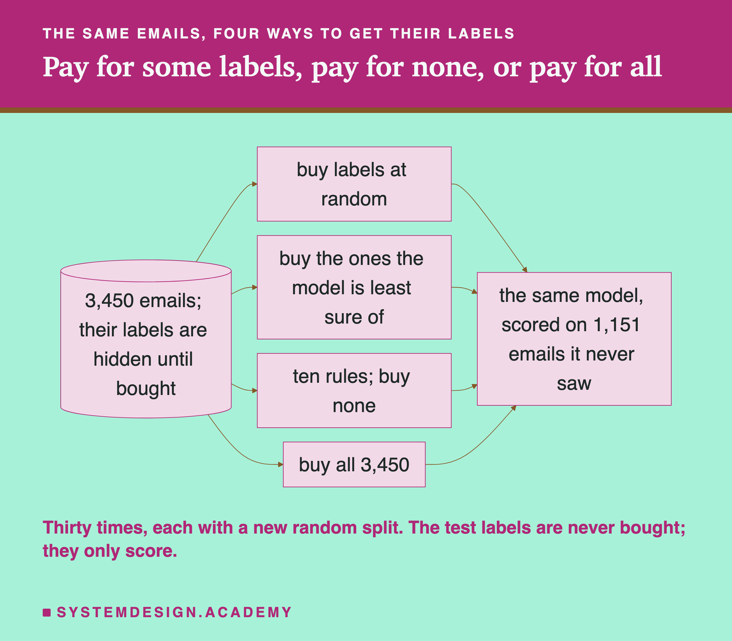
The flowchart is the plan for the lab. On the left is a pool of 3,450 emails whose answers are hidden until I pay for them. Four arrows leave it: buy answers at random, buy the ones the model is least sure of, let ten rules answer and buy none, or buy all 3,450. All four feed the same model, and that model is always scored on the same 1,151 emails it never saw. Only the way of getting the answers changes, so any difference in the score comes from that.
Here is the order of the lesson. First the words. Then what a label is, why some cost far more than others, and why even trained people disagree. Then who does the labelling, what it costs, and how teams check it. Then the two ideas this lesson measures: rules instead of people, and asking only about the hard cases. Then the lab, its results, and what I found when I looked closer. Last, model pre-labelling, labels that change their meaning, and what real teams have published.
Ten Words for This Lesson
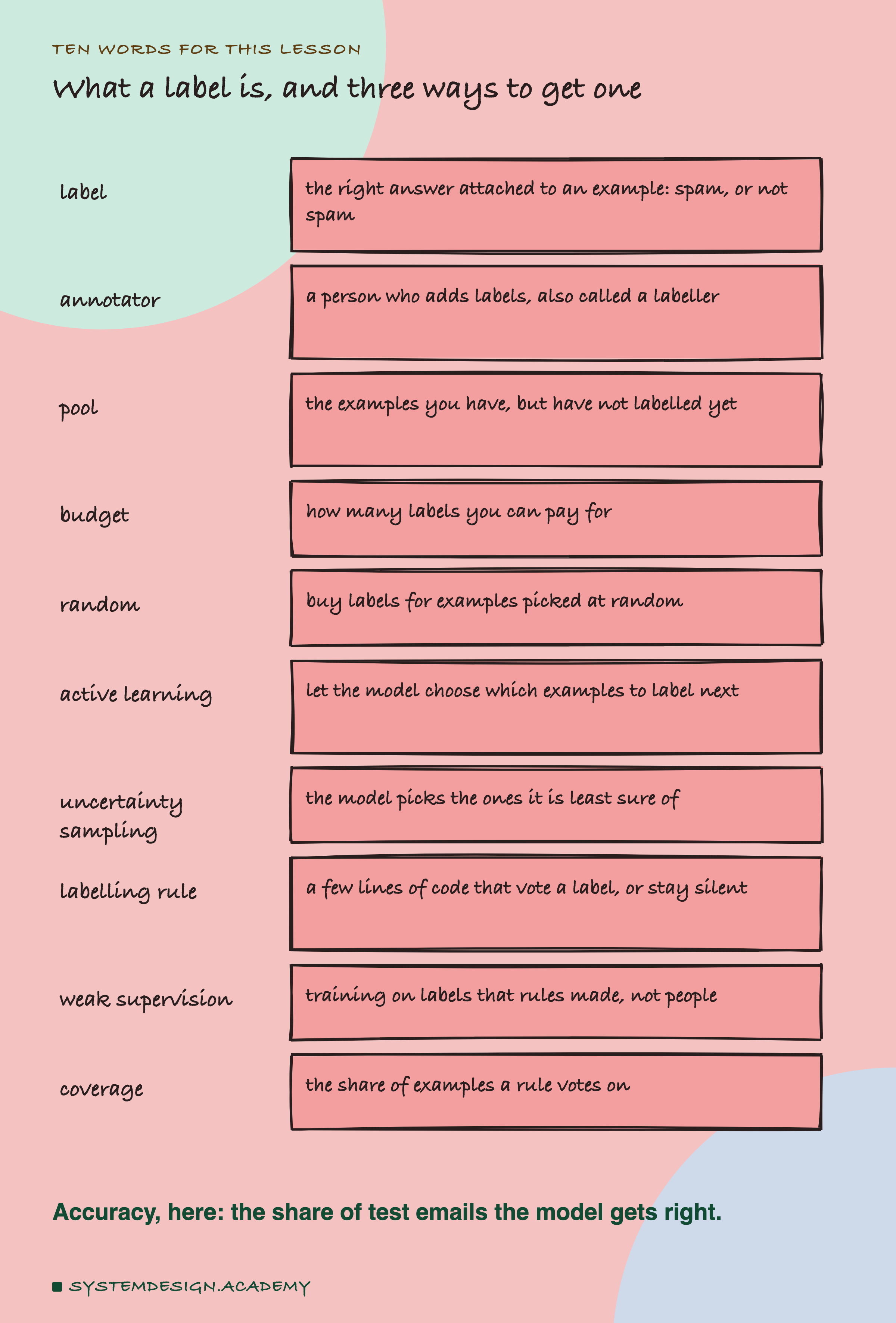
A label is the right answer attached to an example. Here the examples are emails and the label is spam or not spam. Supervised learning is the kind of machine learning that learns from labelled examples, and it is the kind this lesson is about. An annotator, or labeller, is the person who adds the labels.
The pool is every example you have but have not labelled yet. The budget is how many labels you can pay for. Random labelling means buying labels for examples picked at random from the pool, which is what most teams do without thinking about it.
Active learning means letting the model choose which examples a person labels next. The simplest way is uncertainty sampling: the model scores every unlabelled example, and a person labels the ones it is least sure about. For a spam model that gives each email a chance of being spam between 0 and 1, the least sure are the emails nearest 0.5.
A labelling rule, which Snorkel's papers call a labelling function, is a few lines of code that look at one example and vote a label, or stay silent. Weak supervision means training a model on labels that rules made instead of people. A rule's coverage is the share of examples it votes on at all.
Throughout the lab, accuracy is the share of test emails the model gets right. A model that always said not spam would score 0.606 here, because 39.4 percent of the emails are spam.
What a Label Is, and Why Some Cost Far More
A model learns by being shown many examples where the right answer is already known, so that it can find the pattern from input to answer. The input is the raw data. The label is the answer attached to it. Without labels, the same raw data is an unsolved problem, which is why labelling comes before almost every supervised project.
The shape of a label depends on the task, and the shape is what drives the cost:
| Task | The raw input | The label a person attaches |
|---|---|---|
| Sentiment | A product review | positive, negative or neutral |
| Image classification | A photo | "cat", "dog" or "neither" |
| Object detection | A street photo | a box around every car and person |
| Segmentation | A street photo | the right class for every pixel |
| Named entities | A sentence | spans marked as person, company, date |
| Speech | An audio clip | the exact words spoken |
People Disagree, Even Trained Ones
Labelling is also hard for a reason that has nothing to do with time: people disagree. Show three people the same slightly rude review and you can get three answers. The question is how often, and the honest answer is that it depends on the task.
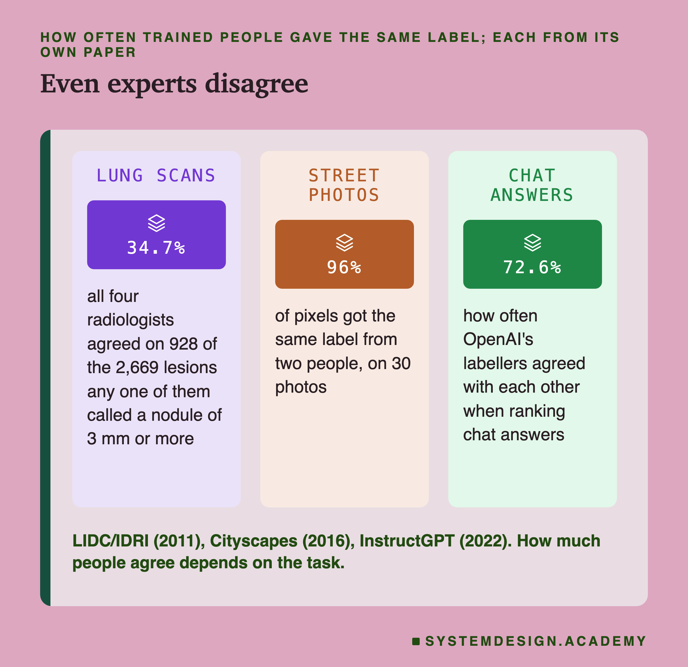
The three panels come from three published datasets. In the LIDC/IDRI lung scan collection, four experienced chest radiologists marked every scan in two reads. First each read it blind, on their own. Then each saw the other three's marks, without names, and gave a final opinion. After that second read, 2,669 lesions were called a nodule of 3 mm or more by at least one of them. All four agreed on 928 of those, which is 34.7 percent.
In Cityscapes, two people labelled the same 30 street photos pixel by pixel, and 96 percent of the pixels got the same label. In OpenAI's InstructGPT work, labellers ranked a model's chat answers from best to worst. The paper reports that they agreed with each other 72.6 percent of the time.
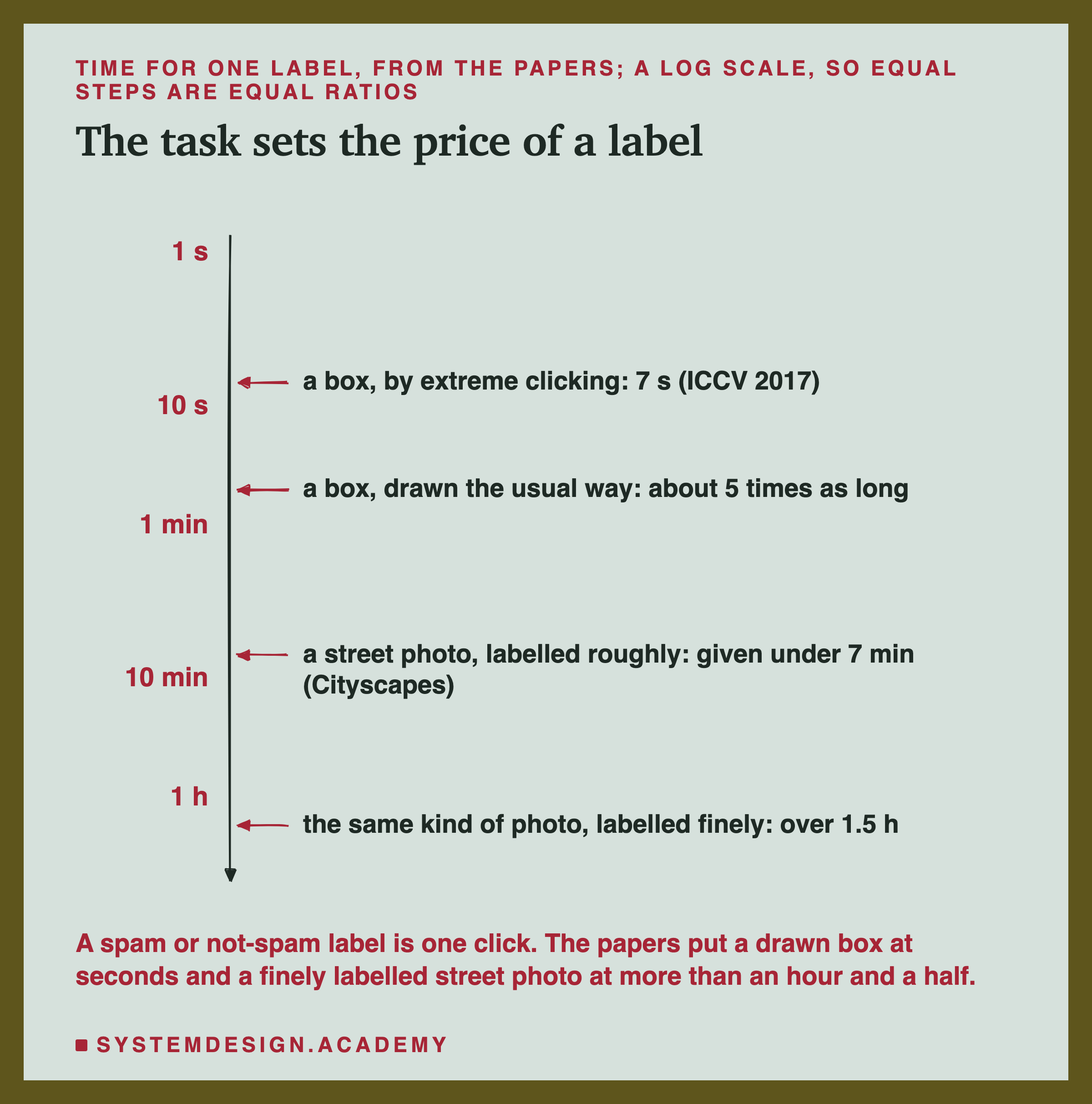
Those three numbers are not a ranking of people. Radiologists are not worse at their job than street-photo labellers. The lung task is harder to define: where a shadow stops being a nodule is a judgement call, and a pixel of road is not. So the first thing to measure on any new labelling job is how often your own people agree, before you pay for thousands of labels.
Raw agreement can flatter you. If two people both say "not spam" to 90 percent of the emails, they will agree often just by luck. Cohen's kappa corrects for that luck when there are two labellers, and Fleiss' kappa does the same when there are more. The evals lesson on inter-annotator agreement compares two graders on the same answers and computes Cohen's kappa by hand, so I do not repeat it here.
What a wrong label does to a model depends on the kind of mistake. Lesson 11, wrong labels, measured, found that some models shrugged off random mistakes. A random forest lost only 3.2 points of accuracy with 40 percent of its labels wrong at random. Mistakes with a pattern, where look-alike digits were swapped, did far more damage from 20 percent up.
Who Does the Labelling, and What It Costs
When a team says "we need to label the data", it is choosing among a few kinds of people, and the choice drives cost, speed and quality.
Your own experts. A radiologist labels scans, a lawyer labels contract clauses, a fraud analyst labels payments. The labels are careful and they cost the most, because an expert's hour is expensive and experts have other work. Teams use them when the task needs real expertise or the data is too private to send outside. Experts also build the small, careful set that everything else is checked against.
A crowd. The work is cut into small tasks and posted on a platform such as Amazon Mechanical Turk, where many people each do a few. It is cheap, fast and large, but you do not know who is on the other end or how carefully they read. The crowd on its own is not reliable. The checks you build around it can be, and the next slide is about those checks.
A labelling company. Scale AI describes its business as "high-quality training data, annotations, and RLHF to power the world's most advanced AI models". RLHF is reinforcement learning from human feedback: people compare a model's answers, and the model is trained toward the ones they prefer. Appen says it has "1M+ vetted contributors worldwide". Labelbox sells labelling software and also an expert network it calls Alignerr. These companies supply the people, the tools and their own checks, and you pay them for not having to run all that yourself.
Crowd platforms publish their fees, so this part of the bill can be computed exactly. The ledger below does it for the lab's 3,450 emails.
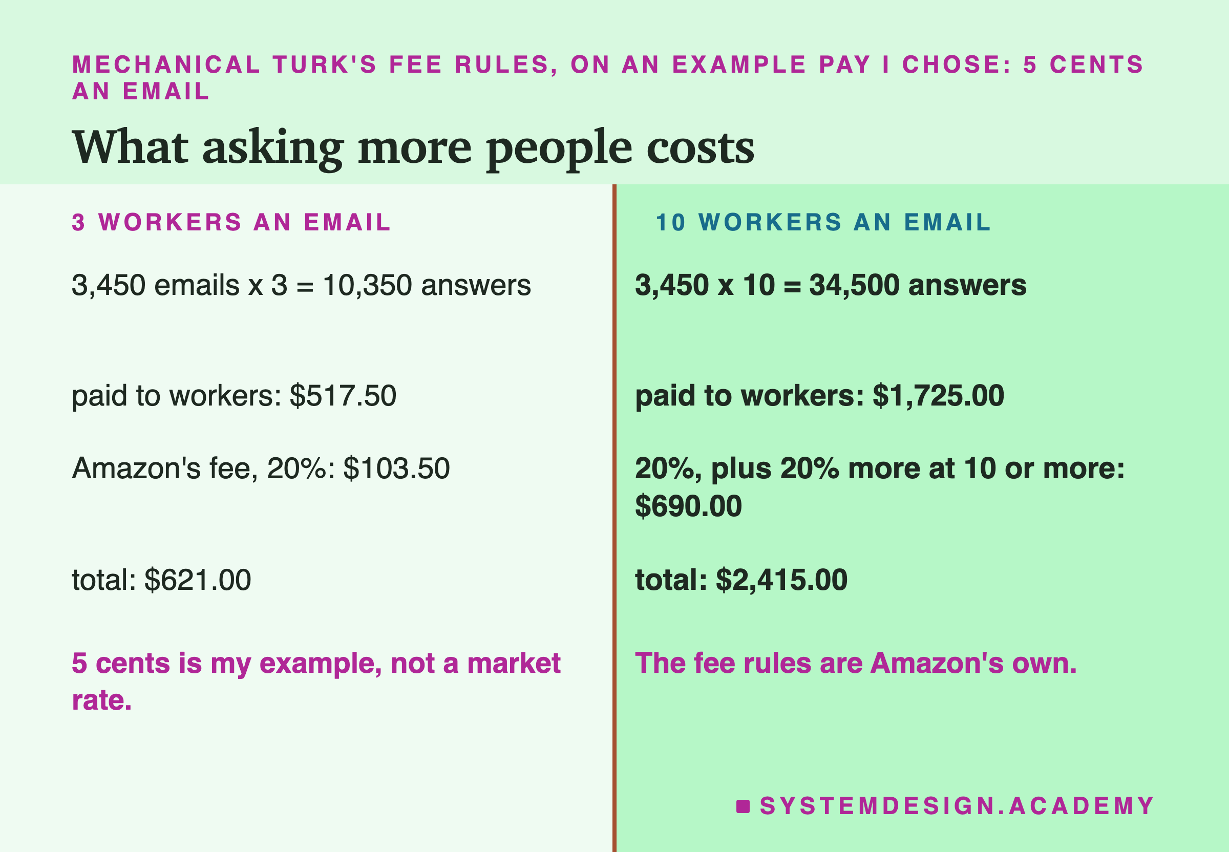
Mechanical Turk's pricing page says Amazon takes a "20% fee on the reward and bonus amount (if any) you pay Workers". It also says "HITs with 10 or more assignments will be charged an additional 20% fee". A HIT is one task, and an assignment is one worker doing it. Asking only for Masters adds 5 percent more. Masters are workers Amazon's own systems picked as high performers across many tasks. The pay per email is your own choice, and I used 5 cents only as an example.
Consensus, Hidden Test Items, and the Rulebook
The idea that makes a crowd usable is to trust the system, not any one person. It is the same idea that makes a reliable service out of machines that sometimes fail. Three checks do most of the work.
means asking several people about the same item and taking the majority. If all three say spam, keep the label. If two say spam and one says not, keep the majority, and send it to an expert when the item matters. In 2008, Snow and colleagues tested Mechanical Turk against expert labels on five language tasks. On one of them, judging the emotion in news headlines, an average of 4 non-expert labels per item matched the quality of one expert. They paid US$2.00 for 7,000 of those labels, about three hundredths of a cent each, a 2008 research rate.
Do not copy that rate. Set the pay per item so that a typical worker earns at least a fair hourly wage. Anthropic's 2022 paper, cited later, says its team kept in touch with its crowdworkers "to ensure that they were being compensated fairly". It also says it aimed to pay them "significantly above the minimum wage in California".
Hidden test items, often called gold questions, are items where you already know the right answer. They are mixed into the work, so the labeller cannot tell which ones they are. Someone who gets them wrong is guessing, has misread the rules, or is a script. You drop their answers before they reach the dataset. These items cost almost nothing, and they catch what consensus would quietly average in.
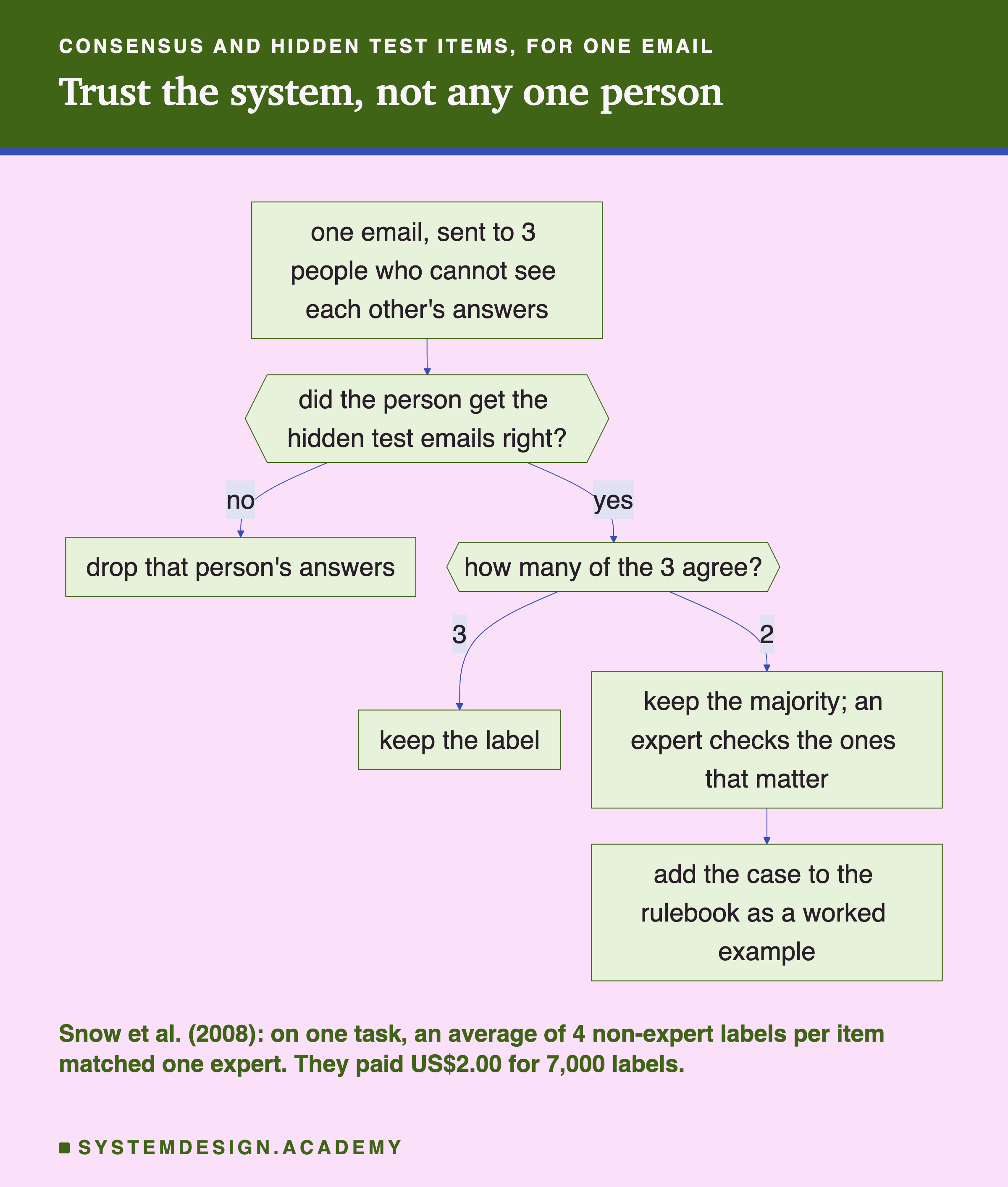
The flowchart shows both checks on one email. The email goes to three people who cannot see each other's answers. Anyone who failed the hidden test items is dropped first. If all three remaining answers agree, the label is kept. If only two agree, the majority is kept and an expert checks the cases that matter. Every such split then goes into the rulebook as a worked example, which is the third check.
The rulebook, or annotation guidelines, is the document that says what each label means and how to handle the hard cases. Teams like to skip it and start labelling, because labelling feels like progress. Then they find out, after paying for ten thousand labels, that half the team read "spam" one way and half another. The hard cases are everywhere. Is a newsletter you signed up for years ago spam? Is a sarcastic review positive or negative? Is a car that is 80 percent hidden behind a lorry worth a box?
Weak Supervision: Rules Instead of Hand Labels
Hand labelling has a ceiling: a person has to look at every item. Weak supervision removes that ceiling. You write a handful of rules and let them label the whole pool. Each rule may be wrong sometimes, and may stay silent when it has nothing to say. Then you train the model on those labels.
The idea got its best-known tool from Stanford. Snorkel was published in 2017 by Ratner, Bach, Ehrenberg, Fries, Wu and Ré. Their paper reports a user study: "subject matter experts build models 2.8x faster and increase predictive performance an average 45.5% versus seven hours of hand labeling". That is their study on their tasks, not a promise for yours.
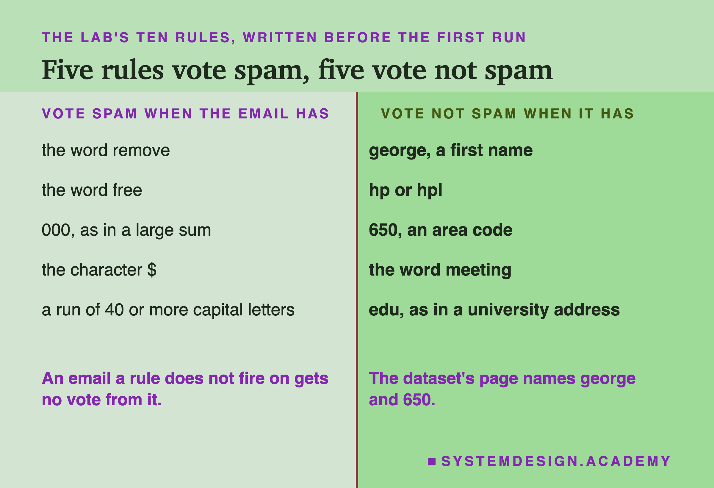
These are the ten rules the lab uses, and I wrote them into the demo's design before its first run. Five vote spam. They fire when an email has "remove", "free", "000" as in a large sum, the character $, or a run of 40 or more capital letters. Five vote not spam when it has "george", "hp" or "hpl", the area code "650", the word "meeting", or "edu" as in a university address. An email a rule does not fire on gets no vote from that rule.
The not-spam rules need a warning. The dataset's own page says its normal emails "came from filed work and personal e-mails". That, it says, is why "george" and the area code "650" mark normal mail. So those rules know whose inbox this is.
The same page says that a filter for everyone would have to "blind such non-spam indicators or get a very wide collection of non-spam". My rules would not carry over to your inbox. They are the email version of "letters that use my boss's first name are real". I also cannot unlearn what I have read about this dataset before, so these are not the rules a newcomer would write.
How do the votes become one label? The simplest way, and the one the lab uses, is a majority vote. Count the spam votes and the not-spam votes, and take the larger. A tie, or no vote at all, means no label, and that email is left out of training.
Snorkel offers something smarter, its LabelModel. Its documentation, which calls the rules labeling functions, or LFs, says it learns "the labeling functions' conditional probabilities of outputting the true (unobserved) label", with no hand labels. It also says it "uses a conditionally independent label model, in which the LFs are assumed to be conditionally independent given Y".
Active Learning: Ask About the Ones It Cannot Decide
If people must label, the question becomes which items are worth their time. Labelling ten thousand easy emails teaches a model almost nothing, because it already gets them right. Active learning lets the model pick the examples that should teach it the most, like the clerk showing her manager only the letters she cannot decide.
Burr Settles's survey of the field calls uncertainty sampling "perhaps the simplest and most commonly used" way, and credits it to Lewis and Gale in 1994. For a model that gives each item a chance between 0 and 1, it "simply queries the instance whose posterior probability of being positive is nearest 0.5". A posterior probability is just the model's chance after it has seen the item.
With three or more classes there are three common versions. One takes the item whose top class is least likely. One takes the smallest gap between the top two classes. One takes the most spread-out chances. For two classes, the survey notes, all three pick the same item.
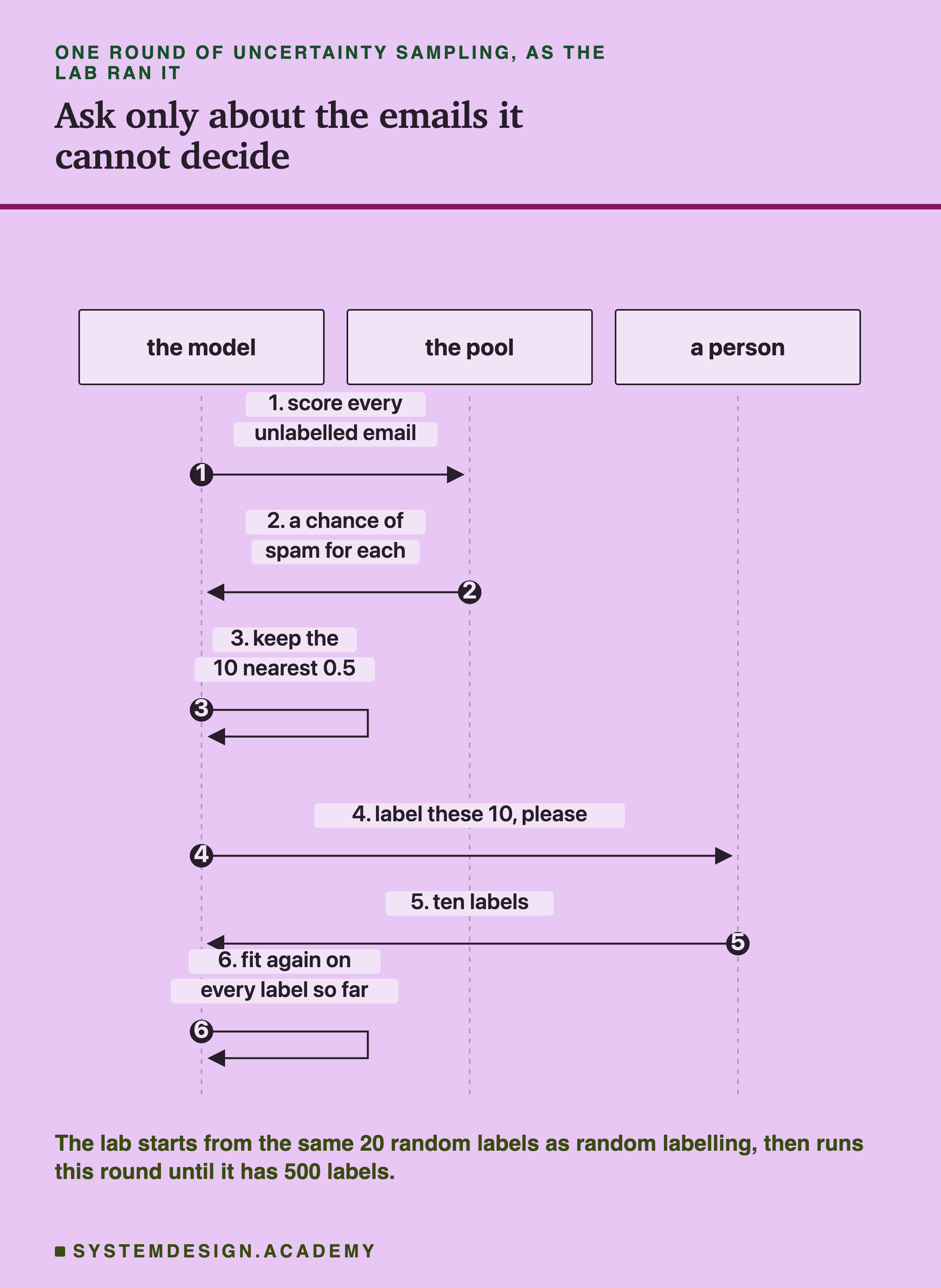
The sequence diagram is one round of the loop as the lab runs it. The model scores every unlabelled email in the pool, and the pool hands back a chance of spam for each. The model keeps the 10 whose chance is nearest 0.5 and asks a person to label those 10. The person sends back ten labels, and the model is fitted again on every label bought so far. Then the round starts again.
How much does this save? The claims range widely. Lewis and Gale wrote that uncertainty sampling "reduced by as much as 500-fold the amount of training data" to be labelled by hand. That was on their text task. Settles's survey also reports the opposite result. Schein and Ungar "showed that active learning can sometimes require more labeled instances than passive learning", using logistic regression, the model this lab uses. Passive learning means labels bought without the model choosing.
What the Lab Ran
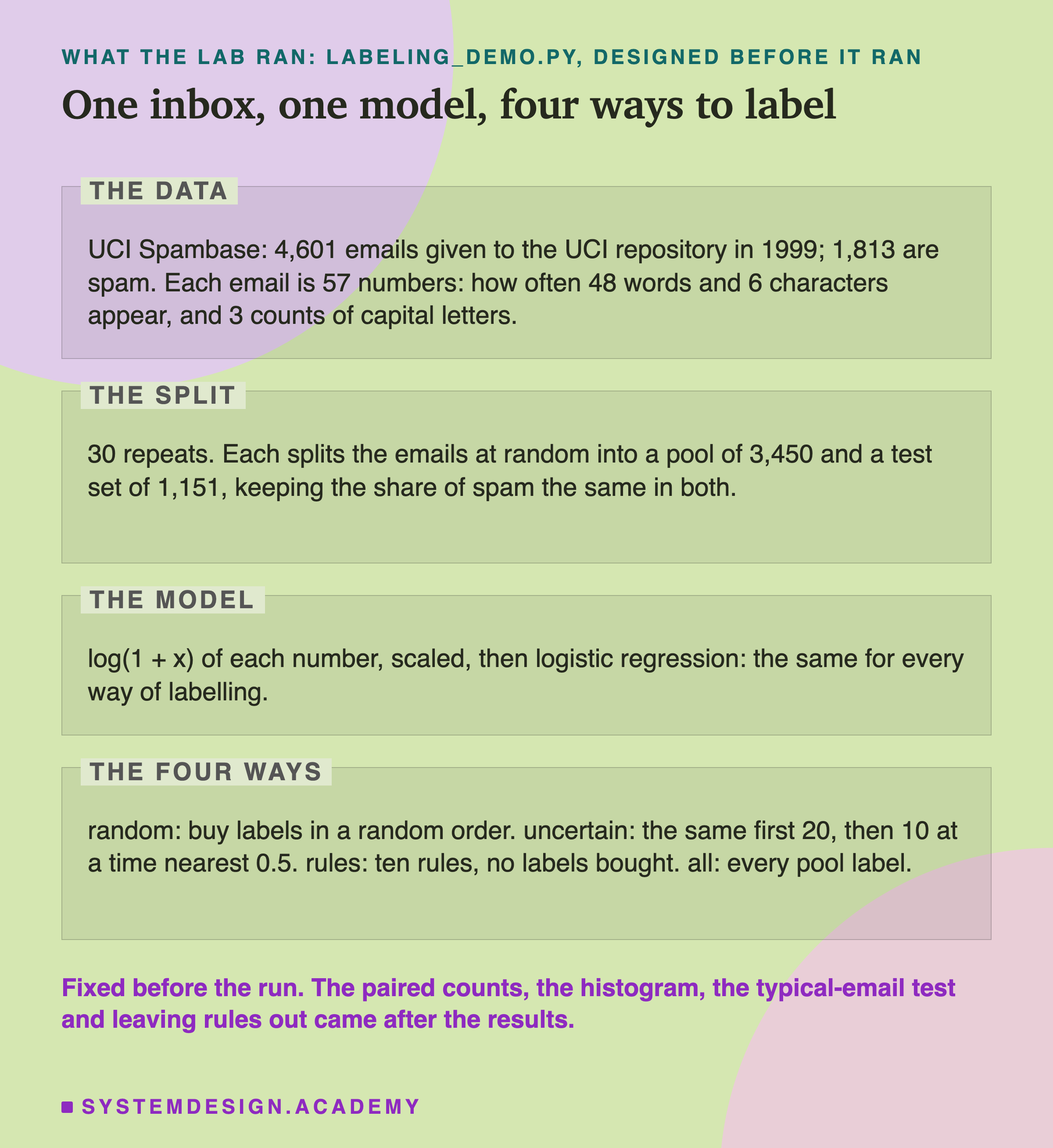
The data. UCI Spambase is 4,601 emails given to the UCI machine learning repository in 1999, and 1,813 of them, 39.4 percent, are spam. The raw text is not included. Each email is 57 numbers. 48 of them say what percentage of its words is each of 48 chosen words. 6 do the same for 6 chosen characters, and 3 count its capital letters. A rule such as "has the word free" becomes "the free number is above zero".
The split. Each of the 30 repeats splits the emails at random into a pool of 3,450 and a test set of 1,151.
Each repeat has its own random-number seed, s from 0 to 29 in the code, which fixes its split and its random order. That seed is a number, not a set of labels. The share of spam is kept the same in both. The pool plays the unlabelled emails: a strategy sees a pool label only after it pays for it. The test labels are never bought. They only score the model at the end, and every strategy on a repeat is scored on the same 1,151 emails.
The model. Every strategy uses the same model. Each number is replaced by log(1 + x), which pulls in the very large counts. Then the numbers are scaled to a similar size and fed to logistic regression. Logistic regression draws one straight boundary through the 57 numbers and turns the distance from it into a chance of spam. I used scikit-learn's defaults except max_iter, which I raised to 2000 so that it always finishes.
The four ways. Random buys labels in a random order of the pool. Uncertain buys the same first 20 labels as random, its seed set: the first labels bought at random, before the model chooses. Then it buys 10 at a time: the 10 unlabelled emails whose chance of spam is nearest 0.5. It fits the model again after each 10. Rules buys nothing and trains on the ten rules' majority vote. All buys every pool label, which is the most this pool can teach this model. Random and uncertain are measured at every budget from 20 to 500 labels.
Accuracy Against Labels Bought
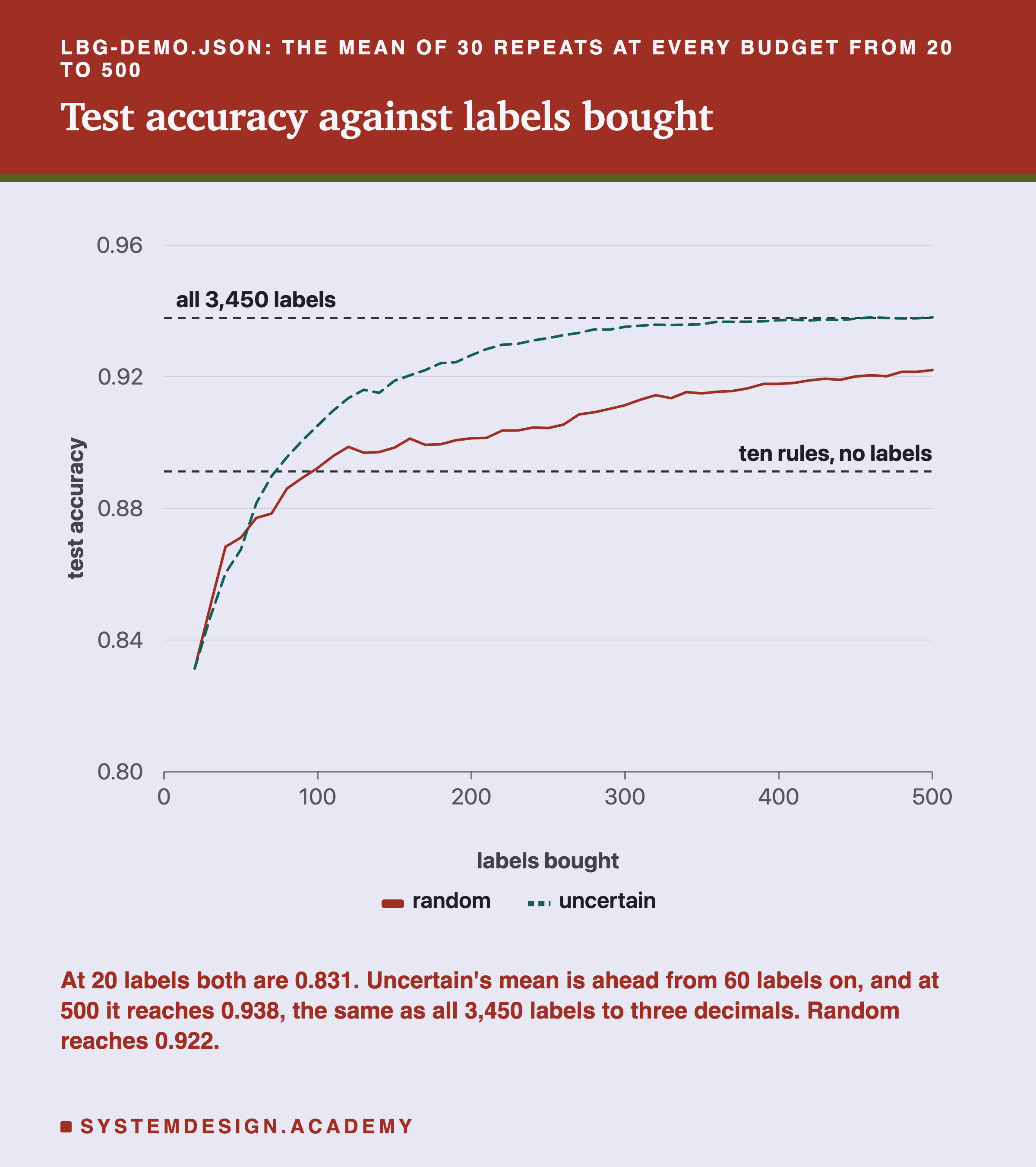
The two lines are the mean of 30 repeats at every budget. At 20 labels both are 0.831, because both strategies hold the same 20 random emails. Then they separate. Uncertain's mean falls a little behind at 30, 40 and 50 labels, and from 60 labels on it stays ahead. By 500 labels it reaches 0.938, the same to three decimals as the model given all 3,450 labels. Random, at 500, reaches 0.922.
The two dashed lines are the fixed marks. The top one is all 3,450 labels at 0.938. The lower one is the ten rules with no hand labels at all, 0.891. Random labelling needs about 100 bought labels before its mean passes the rules. Uncertain passes them sooner, but only after its slow start.
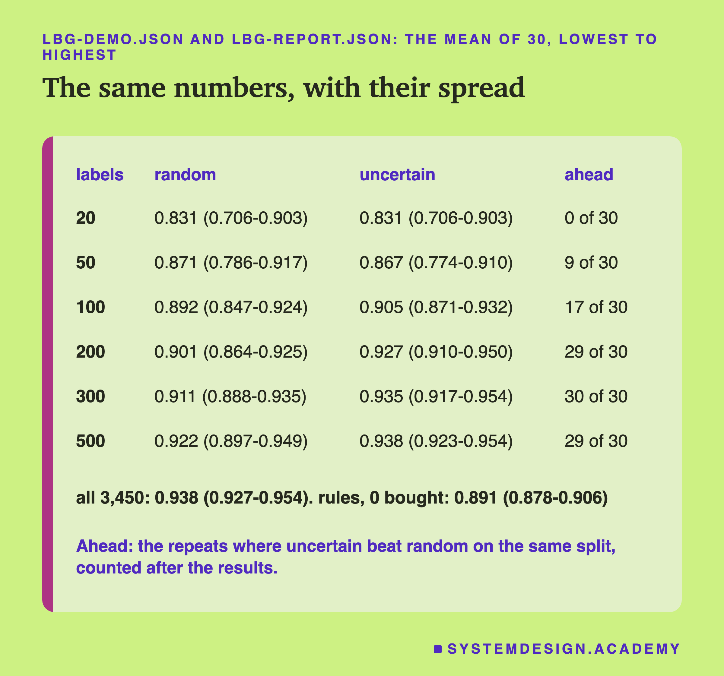
The table shows the spread behind the means, the lowest and highest of the 30 repeats. At 100 labels random ranged from 0.847 to 0.924, and uncertain from 0.871 to 0.932. At 300 labels, uncertain's worst repeat, 0.917, was above random's mean, 0.911. At 500, uncertain ranged from 0.923 to 0.954, which is almost exactly the range of the model given every label, 0.927 to 0.954.
So on this data, with this model, aiming the labels bought the accuracy of the full pool for 500 of its 3,450 labels, about one in seven. Buying at random did not get there by 500. The next slides ask whether that could be luck and where the slow start came from. Then they show a cost of the aimed labels that the accuracy line hides.
Thirty Repeats, Not One
A single random split can tell almost any story. At 20 labels, one repeat scored 0.706 and another 0.903, on the same kind of emails with the same model. If I had run the lab once, the headline would have been whatever that one split said. So I ran it 30 times, and after seeing the means I also counted, repeat by repeat, how often the aimed labels won.
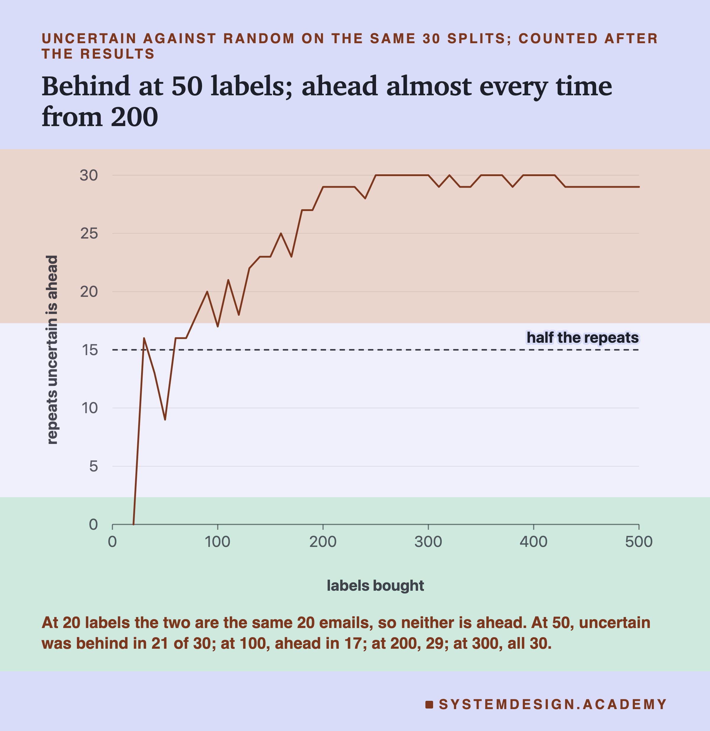
The line counts, at each budget, the repeats in which uncertain scored higher than random on the same split. At 20 labels it is zero, because the two are identical. At 50 labels uncertain was behind in 21 of 30 repeats, with a mean gap of -0.004. At 100 it was ahead in 17 and behind in 13, close to a coin toss, even though its mean was 0.013 higher. At 200 it was ahead in 29 of 30, at 300 in all 30, and at 500 in 29.
The slow start has a simple possible reason, which I did not test. With 20 labels the model is poor, so its idea of "the emails nearest 0.5" is poor too. It spends its next labels on emails that only a poor model finds confusing. Random labels at least cover the pool evenly. Once the model is decent, its doubts point at the right emails.
The practical lesson is to never trust one run of a comparison like this. A difference of 0.013 at 100 labels was a mean over 30 repeats that split 17 to 13. On one repeat it could have pointed either way.
How Many Labels to Get Close to All of Them
A second way to read the curves is to fix a target and count the labels needed to reach it. I set the target before the run: the accuracy of the model given all 3,450 labels on the same repeat, minus 0.01. That is one point of accuracy below the best this pool can do.
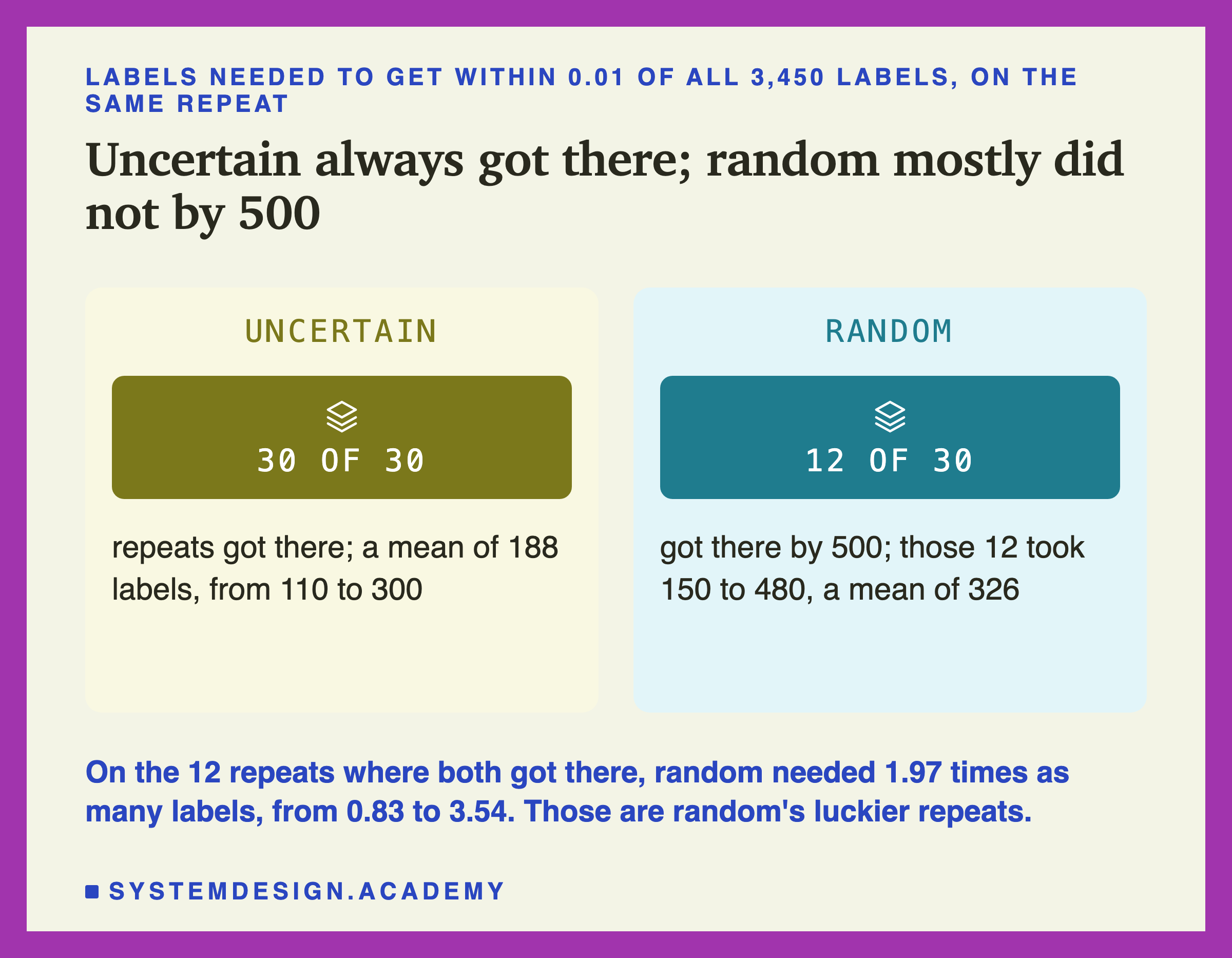
Uncertain reached the target in all 30 repeats, with a mean of 188 labels and a range from 110 to 300. Random reached it by 500 labels in only 12 of the 30 repeats. In the other 18 it had not got there when the budget ran out, so its true count on those is somewhere above 500. On the 12 where it did, it took from 150 to 480 labels, a mean of 326.
The panel also gives a ratio, and it needs care. On the 12 repeats where both reached the target, random needed 1.97 times as many labels, from 0.83 to 3.54. Those 12 are random's luckier repeats, the ones where it got there early.
The other 18 can be bounded. There random needed at least 510 labels, so its ratio was at least 510 divided by uncertain's count on that repeat. After the review of this lesson, the report computed those 18 bounds: 17 of them are above 1.97. Counting each of the 18 at its bound, the ratio over all 30 repeats is at least 2.46. So "about twice as many" understates it.
Compare that with the published claims. Lewis and Gale reported up to 500 times fewer labels on their text task. Schein and Ungar found cases where active learning needed more. Here it was at least about twice, on one inbox with one model. Your data may land anywhere in that range, which is the reason to measure it on your own.
What Uncertainty Sampling Looked At
To see why aiming works, I looked inside one round. After the results, I took repeat 0 and looked at the model when it had 100 labels. I chose repeat 0 because it is the first, not because of what it showed. It had 3,350 emails left to choose from.
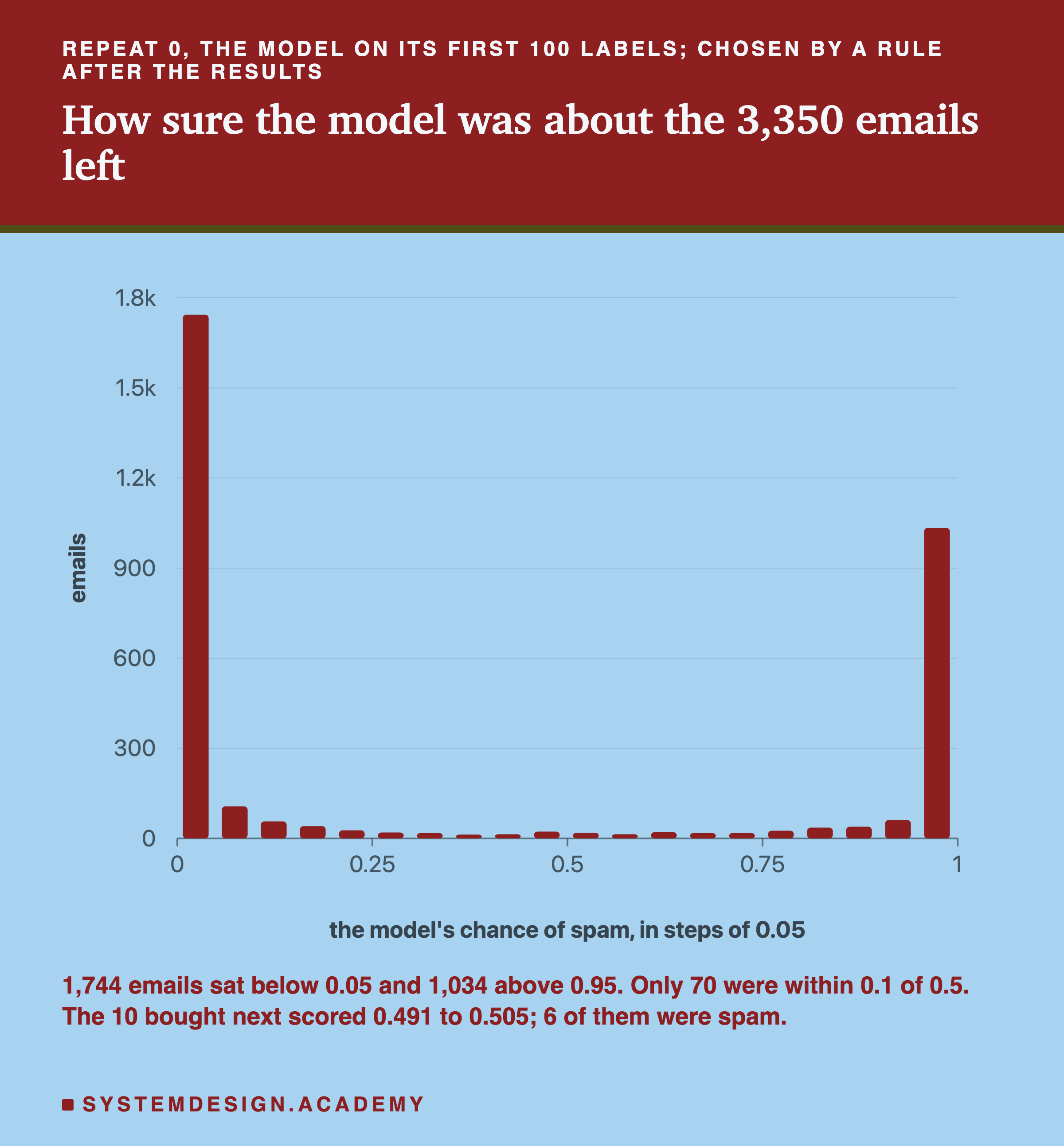
The bars count those 3,350 emails by the model's chance of spam, in steps of 0.05. Almost all of them are piled at the two ends: 1,744 below 0.05 and 1,034 above 0.95. In total 2,946 of the 3,350 scored below 0.1 or above 0.9. Only 70 were within 0.1 of 0.5. With only 100 labels, this model was already sure about most of the inbox, and at that point it had 0.920 accuracy on the test set.
The 10 emails it bought next all scored between 0.491 and 0.505. Six of them turned out to be spam. So the model was right to be unsure: its coin-flip emails were close to half spam. Each of those labels settles a real question for the model. A label on one of the 2,778 emails in the two end bars mostly confirms what it already believed.
This also shows where the cost hides. The emails near 0.5 are the confusing ones, and confusing emails are likely to take a person longer to label. The lab prices every label the same, which the next slides come back to.
The Labels It Bought Are Not a Fair Sample
Active learning buys a biased set of labels on purpose. That is how it works, and it has two costs that the accuracy line does not show.
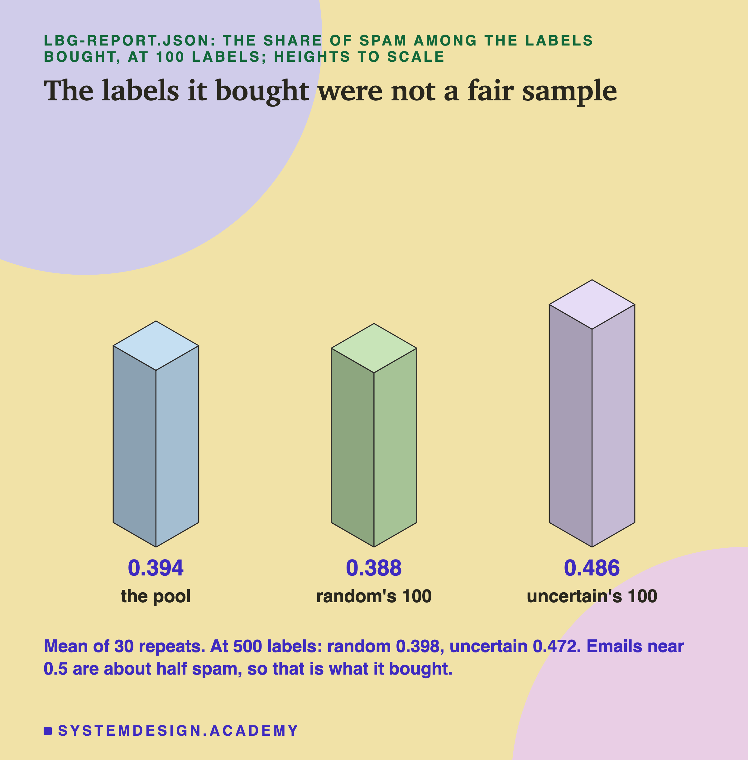
The first cost is the mix. The three blocks are the share of spam in the pool, 0.394, in random's first 100 labels, 0.388, and in uncertain's first 100 labels, 0.486. Random's labels look like the pool, as a random sample should. Uncertain's do not, because emails near 0.5 are about half spam. At 500 labels the shares were 0.398 and 0.472. Count spam in the aimed labels to estimate how much spam you get, and you would be 9 points too high at 100 labels, 8 at 500.
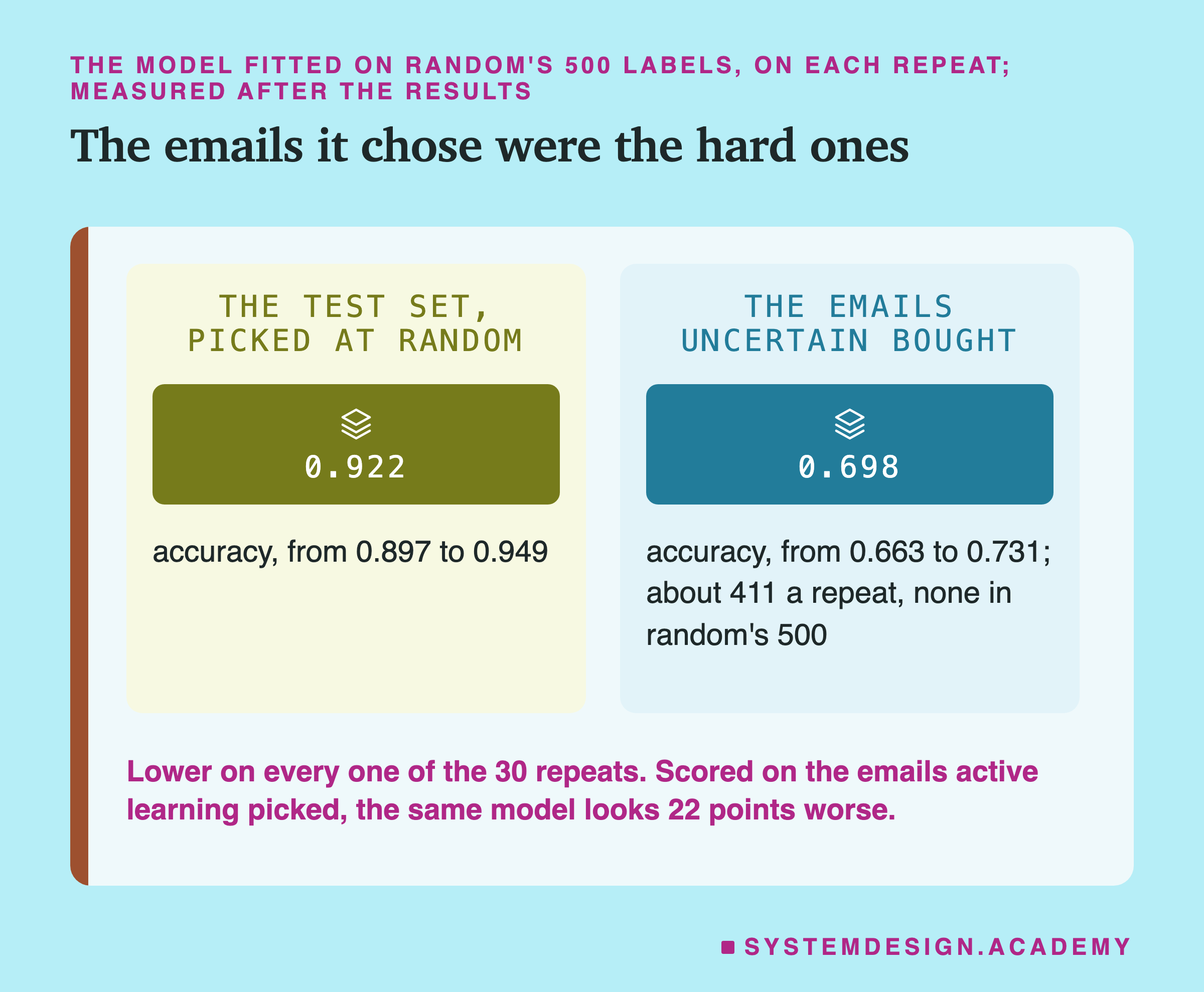
The second cost is harder. I took the model fitted on random's first 500 labels and scored it twice on each repeat. Once on the random test set, and once on the emails uncertain had bought that random had not, about 411 a repeat. On the test set it scored 0.922. On the emails active learning picked, it scored 0.698. It was lower on every one of the 30 repeats. I designed this check after the results, to test a worry, and the worry held.
The lesson is plain. Never use actively chosen labels as your test set, and never report accuracy measured on them. They are the hard emails by design, so they make any model look worse than it is. If you tune a model on them, you tune it for the edge of the problem. Settles's survey says the same in general terms: "the labeled instances are a biased distribution, not drawn i.i.d. from the underlying natural density", where i.i.d. means drawn independently from the same distribution, like fair random draws. Keep a random, carefully labelled test set that no strategy chooses.
Ten Rules, No Hand Labels
The rules strategy bought no labels at all, and it scored 0.891 on average. That is about what random labelling reached with 100 bought labels. To see how, I looked at each rule on all 4,601 emails, against the true labels.
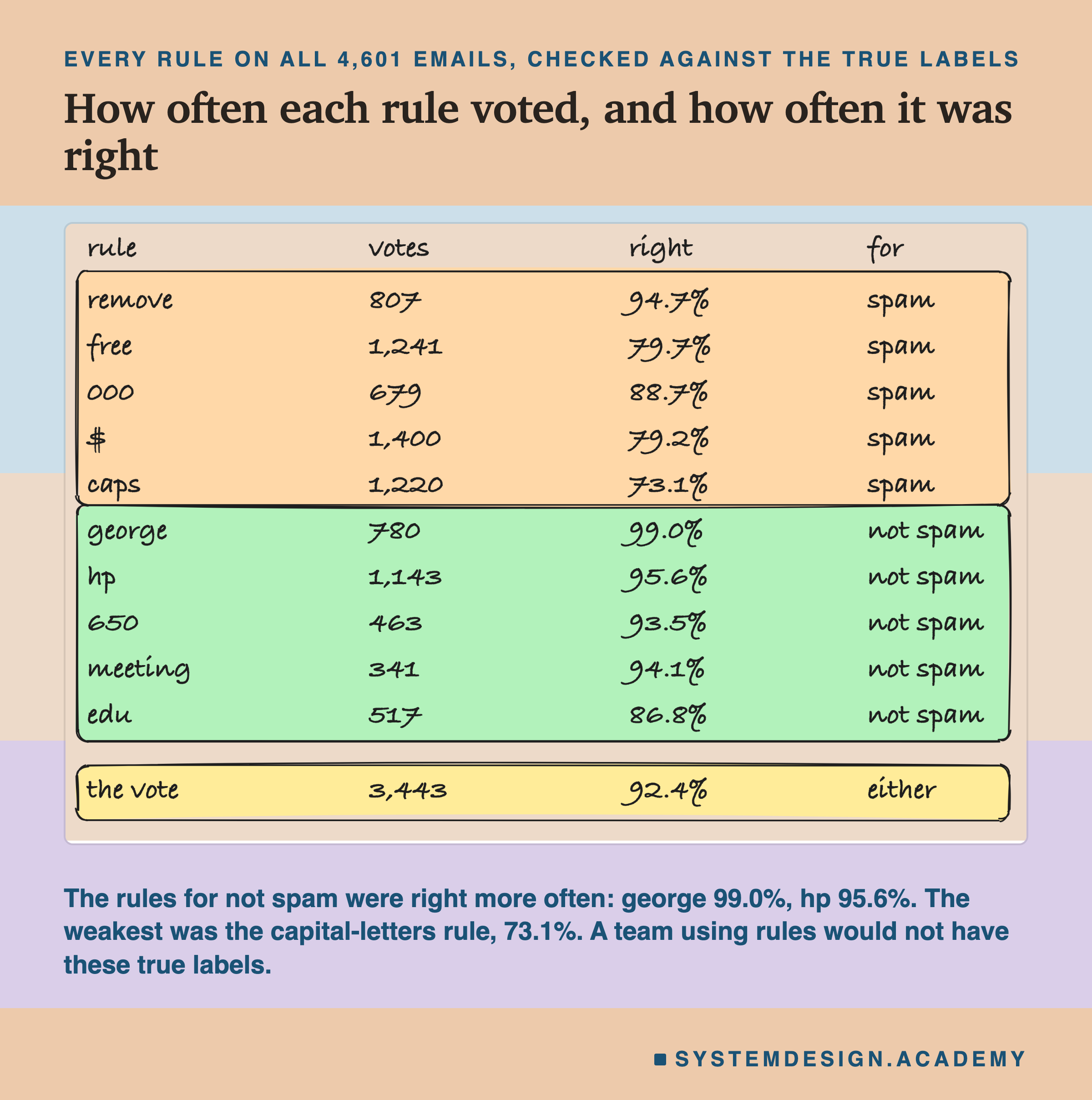
The sketch lists every rule with the number of emails it voted on and the share of those it got right. The not-spam rules were right more often: "george" 99.0 percent of the 780 emails it voted on, "hp" 95.6 percent. The spam rules were weaker, with "free" at 79.7 percent and "$" at 79.2 percent, and the weakest was the capital-letters rule at 73.1 percent. A team using real rules would not have these true labels. It would check each rule on a small hand-labelled sample instead.
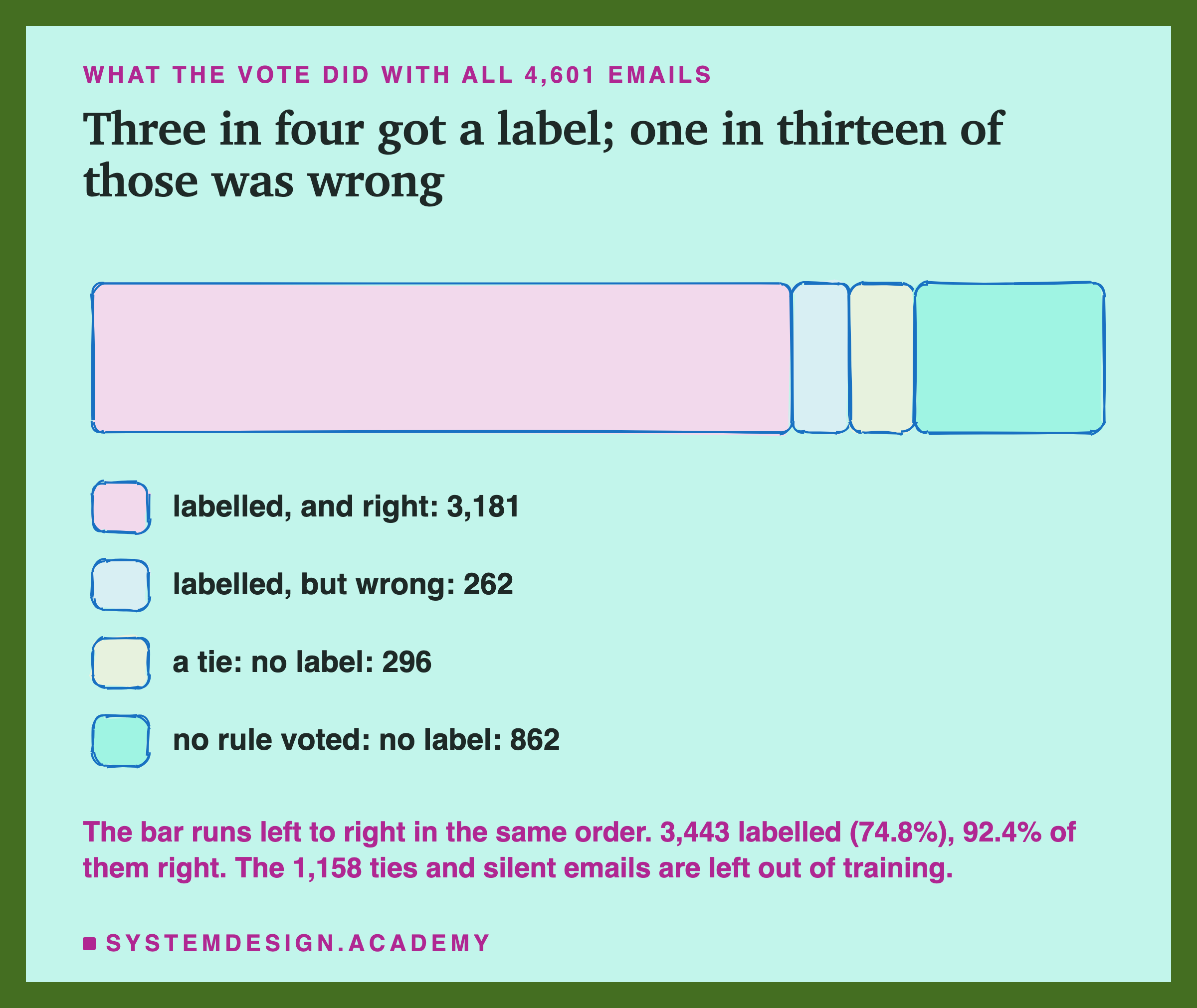
The bar shows what the majority vote did with all 4,601 emails. It gave a label to 3,443 of them, 74.8 percent, and 3,181 of those, 92.4 percent, were right. 262 got the wrong label. 296 were ties, where as many rules voted spam as not spam, and 862 got no vote at all. On each repeat the model trained on about 2,580 rule-labelled pool emails, with about 8 percent of their labels wrong, and still reached 0.891.
Letting a Model Suggest the Label
The newest way to cut labelling cost is to let a large language model make the first pass. It suggests a label for every item, and a person only confirms or corrects it. Checking a suggestion is usually faster than making a label from nothing, when most suggestions are right.
Tools support this directly. Label Studio's documentation says that "if you have predictions generated for your dataset from a model ... you can import the predictions with your dataset into Label Studio for review and correction". The suggestion appears on the labelling screen, and the person edits it instead of starting blank.
How good are such suggestions? One study gives a number. Gilardi, Alizadeh and Kubli published one in 2023 in PNAS, the Proceedings of the National Academy of Sciences.
It used "four samples of tweets and news articles (n = 6,183)". They found that "the zero-shot accuracy of ChatGPT exceeds that of crowd workers by about 25 percentage points on average". Accuracy there means agreement with the authors' own trained annotators, so ChatGPT beat the crowd, not the experts. The cost was "less than $0.003" a label, about thirty times cheaper than Mechanical Turk. Zero-shot means the model was given instructions but no labelled examples. That is one study, on text, with one model version, so treat it as one data point and not a law.
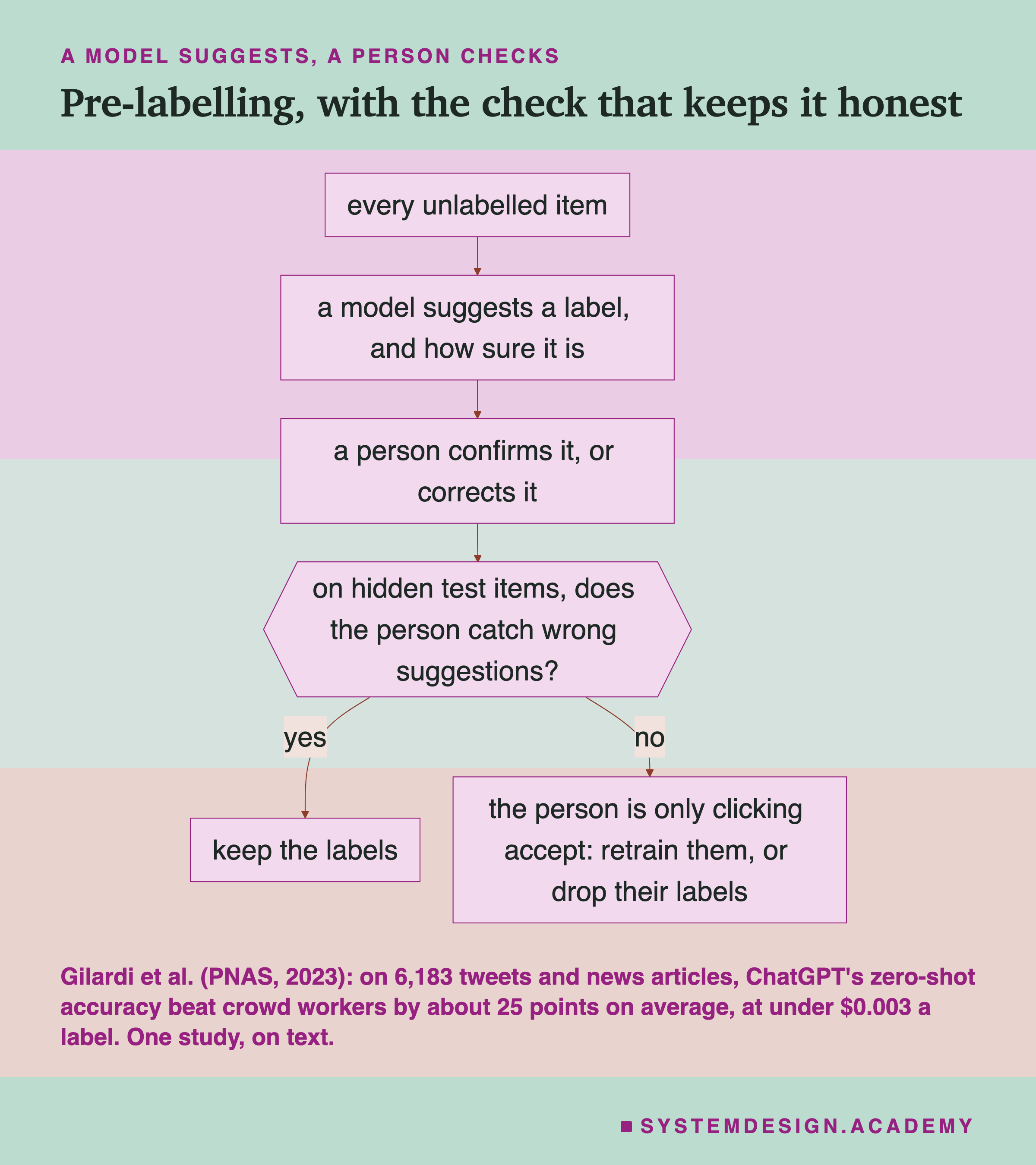
The flowchart adds the check that keeps this honest. Every unlabelled item gets a suggested label and a confidence. A person confirms or corrects it. Then comes the question that matters: on hidden test items where the suggestion is known to be wrong, does the person catch it? If yes, keep their labels. If not, they are only clicking accept, and their labels are the model's labels with a person's name on them.
Respect this risk. A model has its own blind spots. If you accept its labels without a real check, you copy those blind spots into your training data. There they are much harder to find than one person's slip. A confident wrong suggestion is especially easy to wave through. So keep hidden test items running under the checking step too, exactly as for a crowd.
When the Right Answer Changes
Labels are not bought once. Sometimes the meaning of the right answer changes. A new kind of fraud appears that the old "fraud" label never covered. A content policy changes what counts as abusive. A product adds a category that did not exist when you labelled. The emails stay the same, but the correct answer for some of them is now different.
People sometimes call this label drift. The usual name for it is concept drift: the link from input to right answer has moved. Your model was trained on an answer key for a world that has changed, and it gets quietly worse even though its weights never changed. The chapter's lesson on drift alarms measures when a drift alarm means real harm and when it does not.
The fix is relabelling: send a fresh sample of recent data back through the labelling process, often with an updated rulebook, and retrain on it. Mature teams schedule this the way they schedule retraining, because retraining on stale labels only relearns the old world with more confidence.
This is where the cheaper ways earn their keep a second time. A set labelled by rules can be relabelled by changing a rule and running it again. A set labelled by people has to be paid for again. If you kept a random, carefully labelled test set, you can also tell why the model got worse: the world changed, or the new labels are poor.
How Real Teams Describe It
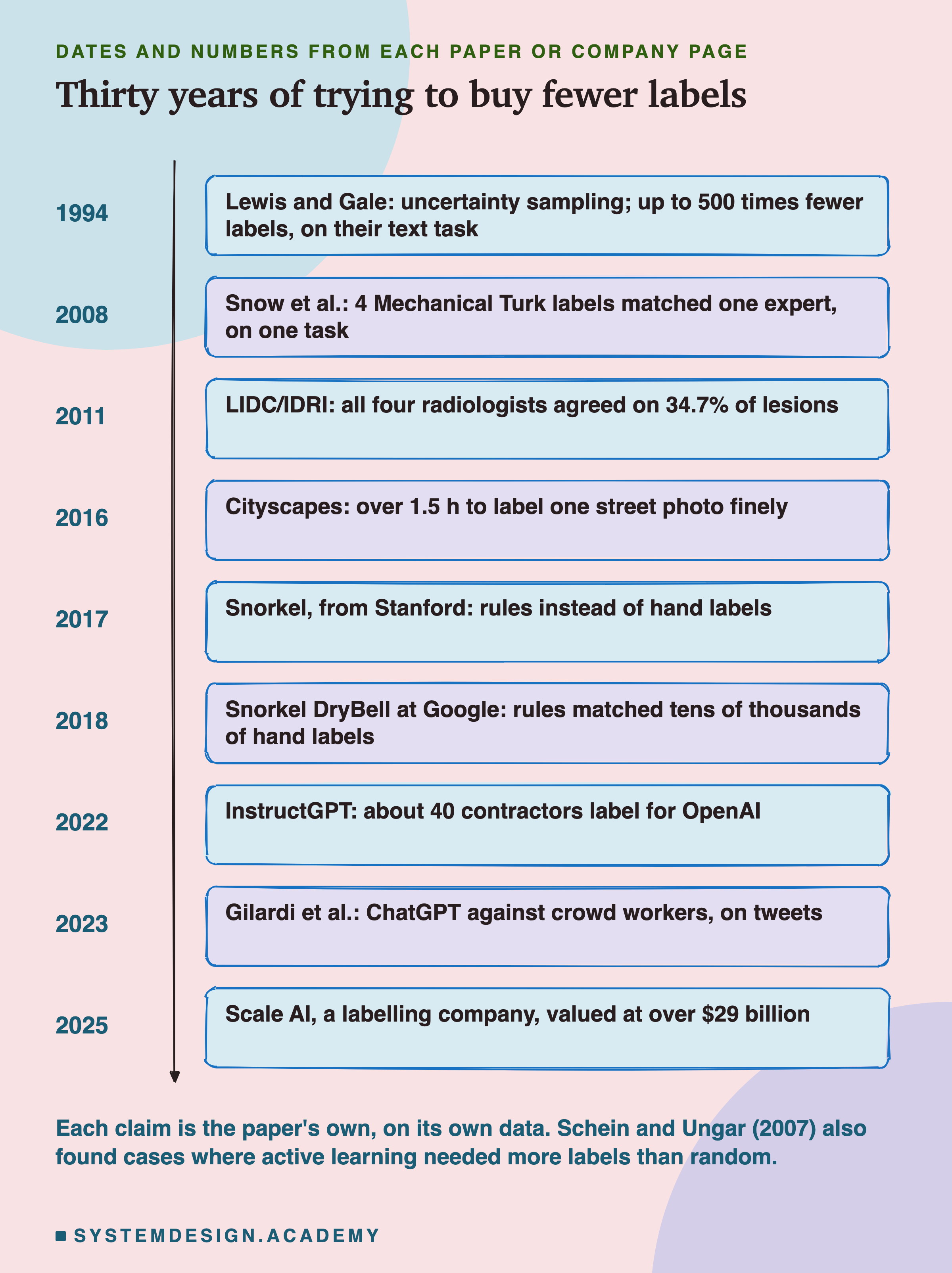
The timeline puts the sources of this lesson in order, each with the number its own paper reports. In 1994 Lewis and Gale introduced uncertainty sampling. In 2008 Snow and colleagues found that 4 Mechanical Turk labels matched one expert on one task. The LIDC/IDRI paper in 2011 reported that all four radiologists agreed on 34.7 percent of lesions. Cityscapes in 2016 measured over 1.5 hours to label one street photo finely.
Snorkel came from Stanford in 2017, and Snorkel DryBell from Google in 2018. InstructGPT's roughly 40 contractors followed in 2022, and Gilardi's study of ChatGPT against crowd workers in 2023. In June 2025 Scale AI, a labelling company, announced an investment from Meta that "values Scale at over $29 billion".
Every one of those claims is about its own data. The line at the bottom of the figure is there for balance: Schein and Ungar found cases where active learning needed more labels than random.
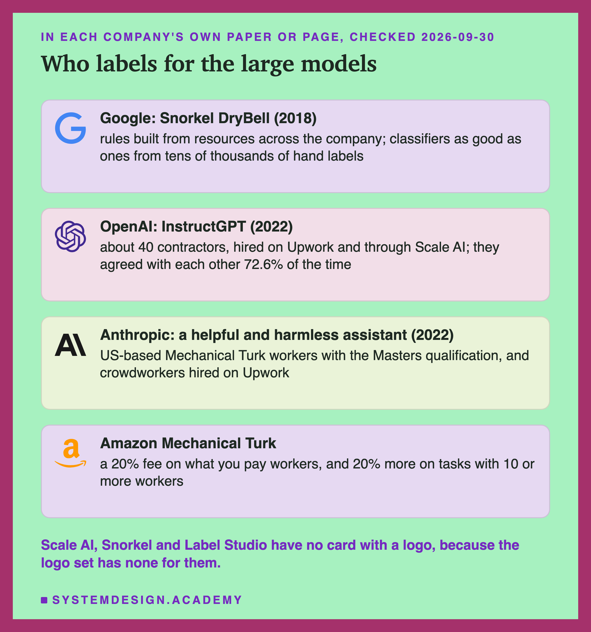
The cards are four companies in their own words. Google's Snorkel DryBell paper says its rules, built from resources across the company, gave classifiers as good as ones trained on tens of thousands of hand labels. OpenAI's InstructGPT paper says "we hired a team of about 40 contractors on Upwork and through ScaleAI". It adds that "training labelers agree with each-other 72.6 ± 1.5% of the time". Anthropic's 2022 paper on a helpful and harmless assistant says it "invited master-qualified US-based MTurk workers" and "also hired crowdworkers on Upwork". Amazon's own page gives Mechanical Turk's fees.
Try It Yourself
This script is the lab. It downloads Spambase and runs the 30 repeats of random and uncertain labelling, from 20 to 500 labels. It fits the rules model and the full-pool model. Then it prints the accuracy table, the labels needed to reach the target, the spam share of the labels bought, and each rule's coverage and accuracy. It needs no GPU. The first time I ran it, it took about 9 seconds after the download. The time depends on the machine and how busy it is, so the script does not print it.
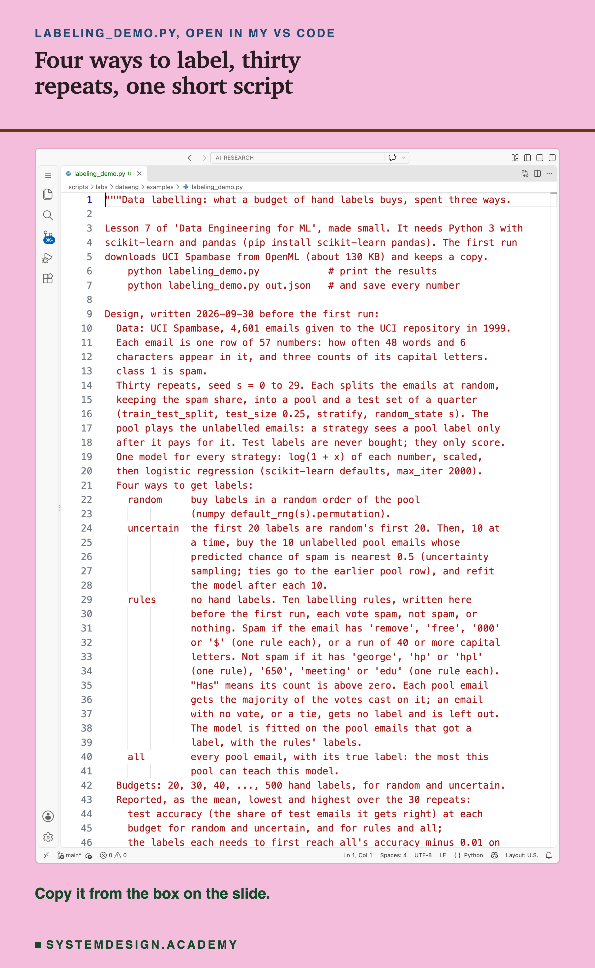
Before you run this lab. You need Python 3 and two libraries: pip install scikit-learn pandas. scikit-learn holds the model and the download, and brings NumPy with it. pandas holds the table the rules read. The first run downloads Spambase from OpenML (about 130 KB), so it needs an internet connection once. After that, scikit-learn keeps a copy in a folder in your home directory (scikit_learn_data).
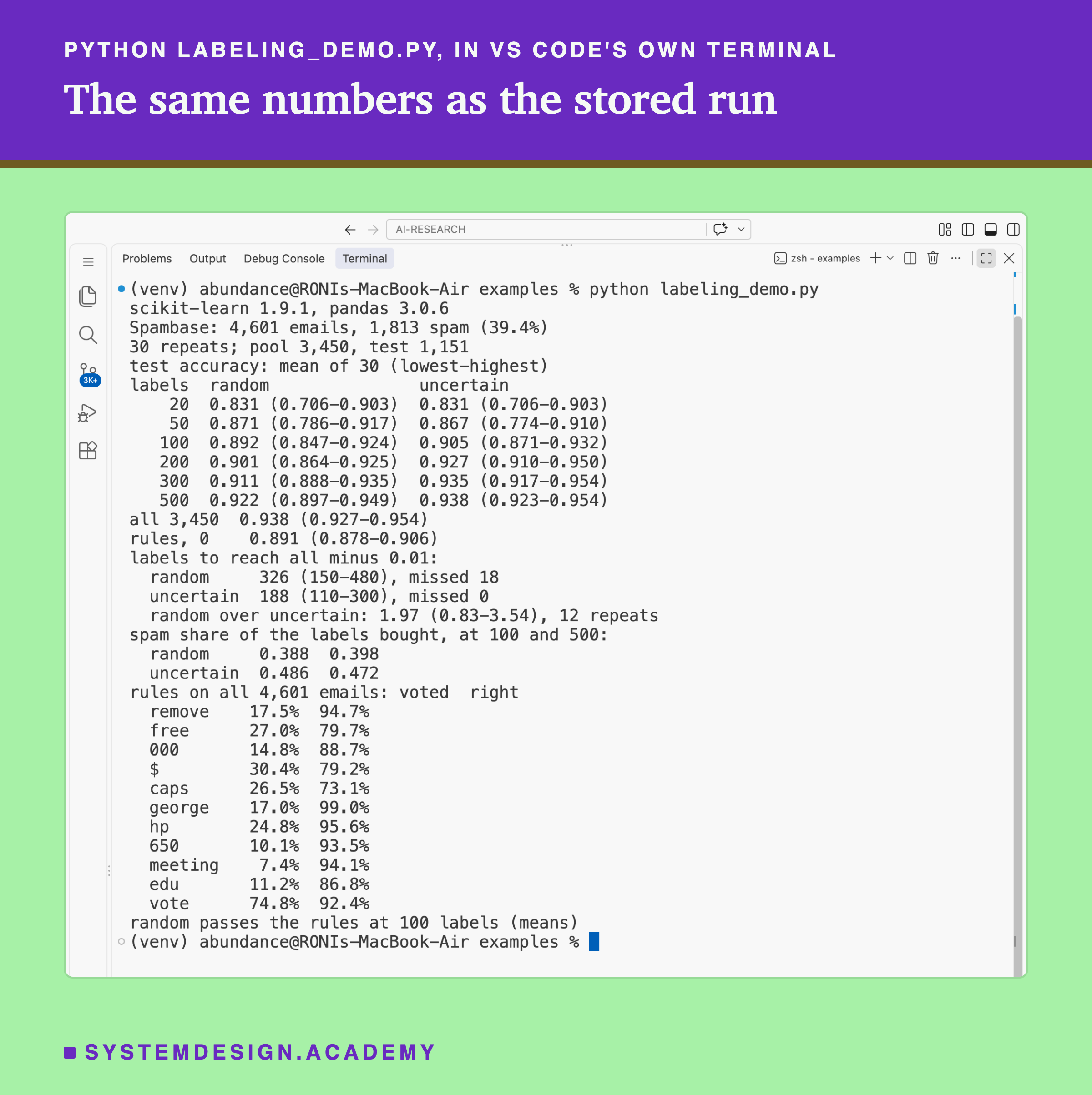
I ran it with scikit-learn 1.9.1 and pandas 3.0.6 on a Mac. scikit-learn runs the same way on Windows and Linux, but I have not checked the numbers there. Another version may give different decimals, so the first line printed is the versions. Give it a file name, python labeling_demo.py out.json, and it also saves every number at full precision. That is how results/lbg-demo.json was made.
"""Data labelling: what a budget of hand labels buys, spent three ways.

Lesson 7 of 'Data Engineering for ML', made small. It needs Python 3 with
scikit-learn and pandas (pip install scikit-learn pandas). The first run
downloads UCI Spambase from OpenML (about 130 KB) and keeps a copy.
    python labeling_demo.py            # print the results
    python labeling_demo.py out.json   # and save every number

Design, written 2026-09-30 before the first run:
  Data: UCI Spambase, 4,601 emails given to the UCI repository in 1999.
  Each email is one row of 57 numbers: how often 48 words and 6
  characters appear in it, and three counts of its capital letters.
  class 1 is spam.
  Thirty repeats, seed s = 0 to 29. Each splits the emails at random,
  keeping the spam share, into a pool and a test set of a quarter
  (train_test_split, test_size 0.25, stratify, random_state s). The
  pool plays the unlabelled emails: a strategy sees a pool label only
  after it pays for it. Test labels are never bought; they only score.
  One model for every strategy: log(1 + x) of each number, scaled,
  then logistic regression (scikit-learn defaults, max_iter 2000).
  Four ways to get labels:
    random     buy labels in a random order of the pool
               (numpy default_rng(s).permutation).
    uncertain  the first 20 labels are random's first 20. Then, 10 at
               a time, buy the 10 unlabelled pool emails whose
               predicted chance of spam is nearest 0.5 (uncertainty
               sampling; ties go to the earlier pool row), and refit
               the model after each 10.
    rules      no hand labels. Ten labelling rules, written here
               before the first run, each vote spam, not spam, or
               nothing. Spam if the email has 'remove', 'free', '000'
               or '$' (one rule each), or a run of 40 or more capital
               letters. Not spam if it has 'george', 'hp' or 'hpl'
               (one rule), '650', 'meeting' or 'edu' (one rule each).
               "Has" means its count is above zero. Each pool email
               gets the majority of the votes cast on it; an email
               with no vote, or a tie, gets no label and is left out.
               The model is fitted on the pool emails that got a
               label, with the rules' labels.
    all        every pool email, with its true label: the most this
               pool can teach this model.
  Budgets: 20, 30, 40, ..., 500 hand labels, for random and uncertain.
  Reported, as the mean, lowest and highest over the 30 repeats:
    test accuracy (the share of test emails it gets right) at each
    budget for random and uncertain, and for rules and all;
    the labels each needs to first reach all's accuracy minus 0.01 on
    the same repeat, and how many repeats never reach it by 500; on
    repeats where both reach it, random's labels over uncertain's;
    the spam share of the labels random and uncertain bought, at 100
    and at 500 labels.
  Over all 4,601 emails: each rule's coverage (the share of emails it
  votes on) and its accuracy on those, checked against the true
  labels, which a team using rules would not have; the vote's
  coverage and accuracy. Last, the smallest budget at which random's
  mean accuracy passes the rules' mean accuracy.
  After the first run, one change, to words only: the data line said
  the emails were "collected at Hewlett-Packard". The dataset's page
  does not say that; it cites a Hewlett-Packard internal report.

Author: Roni Das
Created: 2026-09-30
"""
import json
import sys

import numpy as np
import pandas as pd
import sklearn
from sklearn.datasets import fetch_openml
from sklearn.linear_model import LogisticRegression
from sklearn.model_selection import train_test_split
from sklearn.pipeline import Pipeline, make_pipeline
from sklearn.preprocessing import FunctionTransformer, StandardScaler

REPEATS = 30
FIRST, STEP, MOST = 20, 10, 500
BUDGETS = list(range(FIRST, MOST + 1, STEP))
SHOWN = [20, 50, 100, 200, 300, 500]

raw = fetch_openml(data_id=44, as_frame=True, parser="auto").frame
X = raw.drop(columns="class")
y = (raw["class"].astype(str) == "1").astype(int)


def rule_votes(rows: pd.DataFrame) -> pd.DataFrame:
    """One column per rule: 1 votes spam, 0 votes not spam, -1 no vote."""
    def has(col: str) -> pd.Series:
        return rows[col] > 0
    spam = {"remove": has("word_freq_remove"), "free": has("word_freq_free"),
            "000": has("word_freq_000"), "$": has("char_freq_%24"),
            "caps": rows["capital_run_length_longest"] >= 40}
    ham = {"george": has("word_freq_george"),
           "hp": has("word_freq_hp") | has("word_freq_hpl"),
           "650": has("word_freq_650"), "meeting": has("word_freq_meeting"),
           "edu": has("word_freq_edu")}
    votes = {k: np.where(v, 1, -1) for k, v in spam.items()}
    votes |= {k: np.where(v, 0, -1) for k, v in ham.items()}
    return pd.DataFrame(votes, index=rows.index)


def majority(votes: pd.DataFrame) -> np.ndarray:
    """The majority of the votes cast; -1 for no vote or a tie."""
    n_spam = (votes == 1).sum(axis=1).to_numpy()
    n_ham = (votes == 0).sum(axis=1).to_numpy()
    return np.where(n_spam > n_ham, 1, np.where(n_ham > n_spam, 0, -1))


def model() -> Pipeline:
    return make_pipeline(FunctionTransformer(np.log1p), StandardScaler(),
                         LogisticRegression(max_iter=2000))


def one_repeat(s: int) -> dict:
    Xp, Xt, yp, yt = train_test_split(X, y, test_size=0.25, stratify=y,
                                      random_state=s)
    guess = majority(rule_votes(Xp))
    Xp, Xt, yp, yt = (a.to_numpy() for a in (Xp, Xt, yp, yt))

    def acc(idx: np.ndarray | list) -> float:
        return float(model().fit(Xp[idx], yp[idx]).score(Xt, yt))

    order = np.random.default_rng(s).permutation(len(yp))
    rand = {n: acc(order[:n]) for n in BUDGETS}
    bought = [int(i) for i in order[:FIRST]]
    if len(set(yp[bought])) < 2:
        sys.exit(f"repeat {s}: the first 20 labels hold one class only")
    unc = {}
    while True:
        m = model().fit(Xp[bought], yp[bought])
        unc[len(bought)] = float(m.score(Xt, yt))
        if len(bought) == MOST:
            break
        left = np.setdiff1d(np.arange(len(yp)), bought)
        p = m.predict_proba(Xp[left])[:, 1]
        near = np.argsort(np.abs(p - 0.5), kind="stable")[:STEP]
        bought += [int(i) for i in left[near]]
    keep = guess >= 0
    rules = float(model().fit(Xp[keep], guess[keep]).score(Xt, yt))
    return {"pool": len(yp), "test": len(yt), "all": acc(np.arange(len(yp))),
            "rules": rules, "rules_fitted_on": int(keep.sum()),
            "random": rand, "uncertain": unc, "bought": bought,
            "spam_bought": {k: {n: float(yp[idx[:n]].mean()) for n in (100, MOST)}
                            for k, idx in (("random", order), ("uncertain", bought))}}


def reach(run: dict, kind: str) -> int | None:
    goal = run["all"] - 0.01
    return next((n for n in BUDGETS if run[kind][n] >= goal), None)


def spread(v: list) -> tuple:
    return float(np.mean(v)), float(np.min(v)), float(np.max(v))


def show(v: list, d: int = 3) -> str:
    m, lo, hi = spread(v)
    return f"{m:.{d}f} ({lo:.{d}f}-{hi:.{d}f})"


print(f"scikit-learn {sklearn.__version__}, pandas {pd.__version__}")
print(f"Spambase: {len(y):,} emails, {y.sum():,} spam ({y.mean():.1%})")
runs = [one_repeat(s) for s in range(REPEATS)]
print(f"{REPEATS} repeats; pool {runs[0]['pool']:,}, test {runs[0]['test']:,}")
print("test accuracy: mean of 30 (lowest-highest)")
print(f"{'labels':>6}  {'random':<19}  uncertain")
for n in SHOWN:
    print(f"{n:>6}  {show([r['random'][n] for r in runs])}  "
          f"{show([r['uncertain'][n] for r in runs])}")
print(f"all {runs[0]['pool']:,}  {show([r['all'] for r in runs])}")
print(f"rules, 0    {show([r['rules'] for r in runs])}")

out = {"scikit_learn": sklearn.__version__, "pandas": pd.__version__,
       "emails": len(y), "spam": int(y.sum()), "repeats": REPEATS,
       "budgets": BUDGETS, "runs": runs, "reach": {}, "rules_all": {}}
print("labels to reach all minus 0.01:")
for kind in ("random", "uncertain"):
    got = [reach(r, kind) for r in runs]
    hit = [g for g in got if g is not None]
    out["reach"][kind] = got
    mean = f"{np.mean(hit):.0f} ({min(hit)}-{max(hit)})" if hit else "never"
    print(f"  {kind:<10} {mean}, missed {len(got) - len(hit)}")
both = [(a, b) for a, b in zip(out["reach"]["random"], out["reach"]["uncertain"])
        if a is not None and b is not None]
ratio = [a / b for a, b in both]
out["reach"]["ratio"] = ratio
if ratio:
    print(f"  random over uncertain: {show(ratio, 2)}, {len(both)} repeats")
print("spam share of the labels bought, at 100 and 500:")
for kind in ("random", "uncertain"):
    a = [r["spam_bought"][kind][100] for r in runs]
    b = [r["spam_bought"][kind][MOST] for r in runs]
    print(f"  {kind:<10} {np.mean(a):.3f}  {np.mean(b):.3f}")

votes = rule_votes(X)
print(f"rules on all {len(y):,} emails: voted  right")
for k in votes.columns:
    cast = votes[k] >= 0
    right = float((votes[k][cast] == y[cast]).mean())
    out["rules_all"][k] = {"coverage": float(cast.mean()), "accuracy": right}
    print(f"  {k:<8} {cast.mean():6.1%} {right:6.1%}")
guess = majority(votes)
cast = guess >= 0
out["vote_all"] = {"coverage": float(cast.mean()),
                   "accuracy": float((guess[cast] == y.to_numpy()[cast]).mean())}
print(f"  vote     {cast.mean():6.1%} {out['vote_all']['accuracy']:6.1%}")
rules_mean = np.mean([r["rules"] for r in runs])
passes = next((n for n in BUDGETS
               if np.mean([r["random"][n] for r in runs]) > rules_mean), None)
out["random_passes_rules"] = passes
print(f"random passes the rules at {passes} labels (means)")

if len(sys.argv) > 1:  # a file name was given: save every number too
    json.dump(out, open(sys.argv[1], "w"), indent=1)
The Lab Report
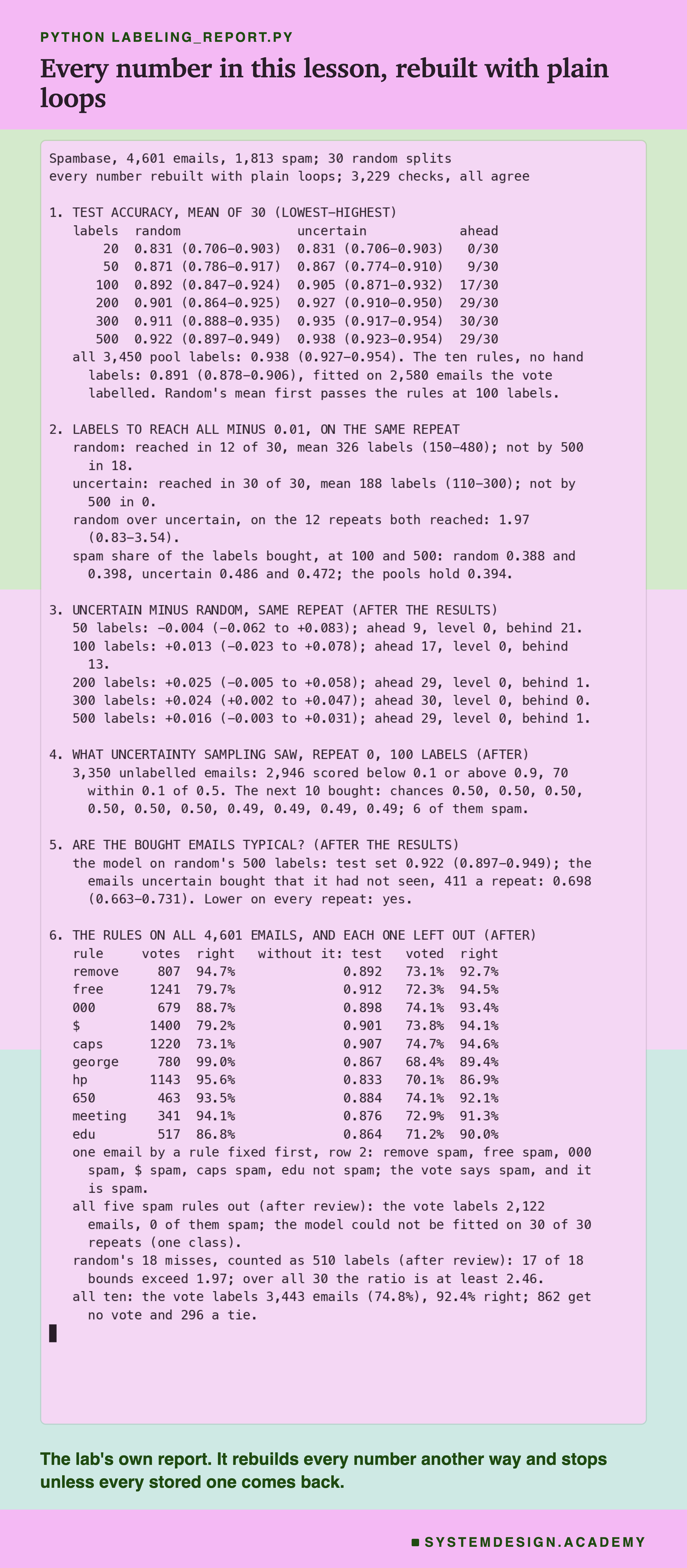
The report lives in scripts/labs/dataeng/labeling_report.py. It reads the demo's stored files, results/lbg-demo.json and the printed run, and Spambase from scikit-learn's local copy. It does not trust the demo's arithmetic. The demo works with pandas tables and NumPy arrays. The report holds the 4,601 emails as plain Python lists and takes log(1 + x) with Python's own math.log1p. It runs the ten rules and the vote with loops, and picks uncertainty sampling's next 10 by sorting in plain Python. It counts every accuracy itself from the model's answers.
It uses the same split, the same random order and the same model as the demo, because those are the design. It stops unless every stored accuracy comes back to within 0.000000000001, every email uncertain bought is the same email, and every rule count is exact. It ran 3,228 checks and all of them agreed. It changes nothing in the demo's files.
Be the Label Model Yourself
This box has no model in it. It holds all 4,601 emails in the dataset's own order. For each one it stores whether the email has each of 23 entries, which are 21 words plus the characters $ and !. It also stores its longest run of capital letters, and whether it is spam. Each email is five characters in base 64, which just means counting with 64 different digits instead of 10, so that the box stays small. It runs in your browser.
The ten rules in it are the lab's rules, exactly as the demo ran them. The report checked that every rule's count, and the vote's, match the demo's stored numbers.
As it is, the box prints each rule's votes and the share it got right. Then it prints the vote: 3,443 emails labelled, 74.8 percent, and 92.4 percent of those right. Those are the numbers on the rules slide.
Now change the rules. Delete the 'free' line and run it again, and watch the vote's accuracy and coverage move. Add a rule of your own, such as 'money': (has('money'), SPAM), or 're': (has('re'), NOT_SPAM),, using any of the 23 entries in WORDS. Change the 40 in the capital-letters rule to 20 or to 60.
One warning. Every time you judge a rule here you are using the true labels, which a real team would not have. Ask yourself which of your changes you could have made without them.
The Vote and the Picks, Worked by Hand
Before you trust a labelling rule, you should be able to apply it with a pencil. So here is one real email, chosen by a rule I fixed before looking at any email. It is the first one, in the dataset's own order, on which the rules vote both ways. That is row 2, the third email.
Row 2 has the word "remove", the word "free", "000" and the character $, and its longest run of capital letters is 485 letters. Each of those five fires a spam rule, so it gets five spam votes. It also has "edu", which fires one not-spam rule. None of the other four not-spam rules fire. Five spam votes against one not-spam vote is a majority for spam, so the vote labels it spam. The true label is spam, so the vote was right.
Now the vote over all 4,601 emails. 862 emails got no vote at all. 296 got as many spam votes as not-spam votes, a tie. That leaves 4,601 minus 862 minus 296, which is 3,443 labelled emails. Their coverage is 3,443 divided by 4,601, which is 0.748. Of the 3,443, 3,181 got the right label, and 3,181 divided by 3,443 is 0.924.
Next, one pick by uncertainty sampling. On repeat 0, with 100 labels, the first email the model bought scored a chance of spam of 0.4993. Its distance from 0.5 is 0.5 minus 0.4993, which is 0.0007. No other unlabelled email was closer. The model sorts all 3,350 unlabelled emails by that distance and buys the 10 smallest.
Last, the bill on the cost slide. 3,450 emails times 3 workers is 10,350 answers. At 5 cents each that is $517.50. Amazon's 20 percent fee is 517.50 times 0.2, which is $103.50, so the total is $621.00. With 10 workers, 34,500 answers cost $1,725.00, the fee is 40 percent, $690.00, and the total is $2,415.00.
The Code, Part by Part
Loading. fetch_openml(data_id=44) downloads Spambase once and reads the local copy after that. X is the 57 numbers of each email, and y is 1 for spam and 0 for not spam.
rule_votes(rows). The ten rules. has(col) is true when a column is above zero. Each spam rule becomes a column that holds 1 where it fires and -1 where it is silent, and each not-spam rule holds 0 where it fires. majority(votes) counts the 1s and the 0s in each row and returns the larger, or -1 for a tie or no vote.
model(). The pipeline every strategy shares: FunctionTransformer(np.log1p) for log(1 + x), StandardScaler() to put the numbers on a similar scale, and LogisticRegression(max_iter=2000).
one_repeat(s). One split, train_test_split(..., test_size=0.25, stratify=y, random_state=s). order is a random order of the pool from default_rng(s). fits the model on the first labels of that order for every budget. The loop is uncertainty sampling. It fits on what has been bought and scores the unlabelled emails with . It sorts them by distance from 0.5, with a stable sort, and buys the first 10. Then fits on the pool emails the vote labelled, and on the whole pool.
How to Spend a Labelling Budget, Step by Step
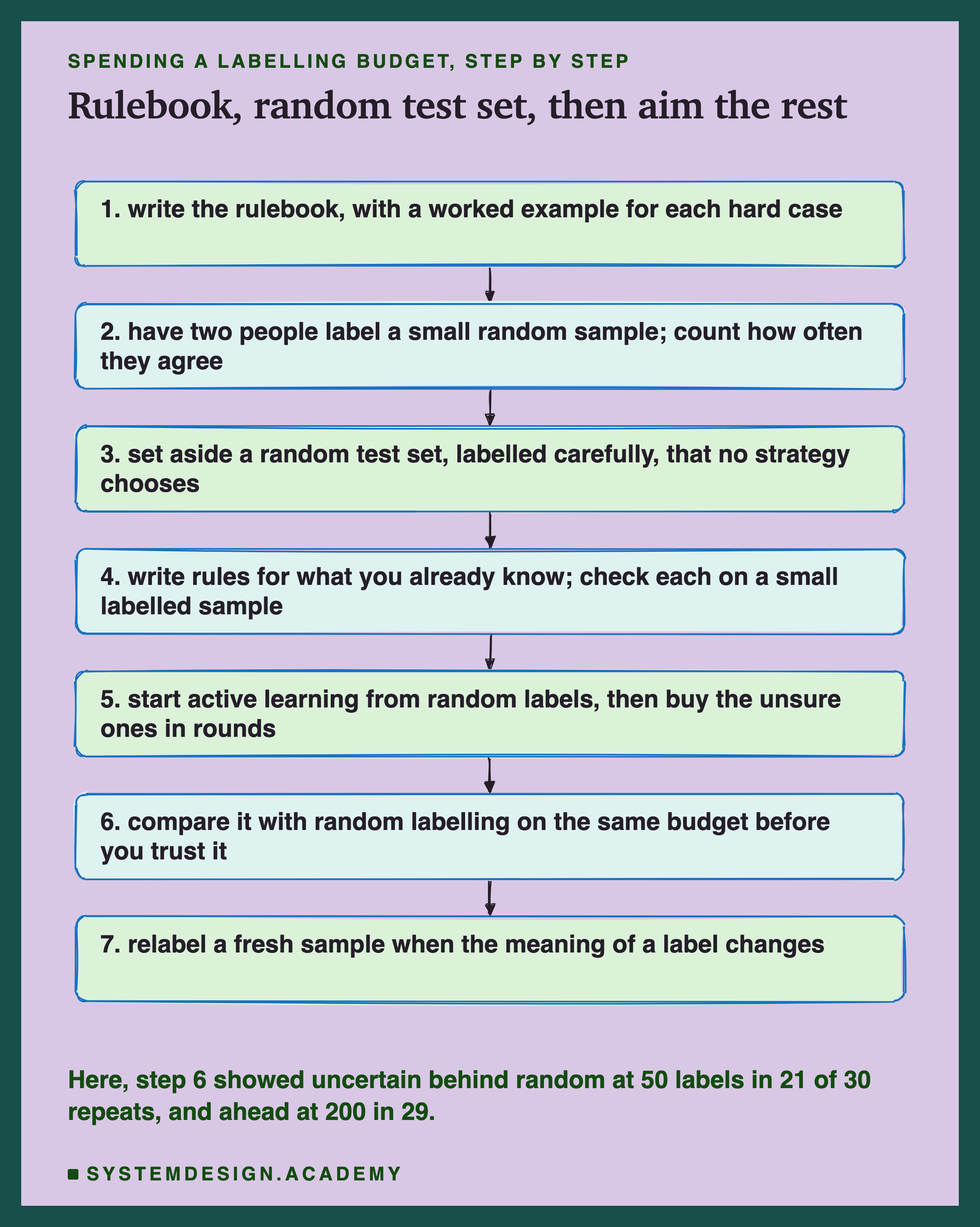
Write the rulebook first. Give every label a definition and every hard case a worked example. It is the cheapest thing on this list, and every later step depends on it.
Measure agreement on a small random sample. Have two people label the same items and count how often they agree. If they rarely agree, fix the rulebook before you buy more labels. The evals lesson shows how to correct that count for luck.
Set aside a random test set. Label it carefully, perhaps with an expert, and never let any strategy choose its items. Here, the emails active learning chose scored 0.698 against 0.922 on a random test set, so a chosen test set would have lied.
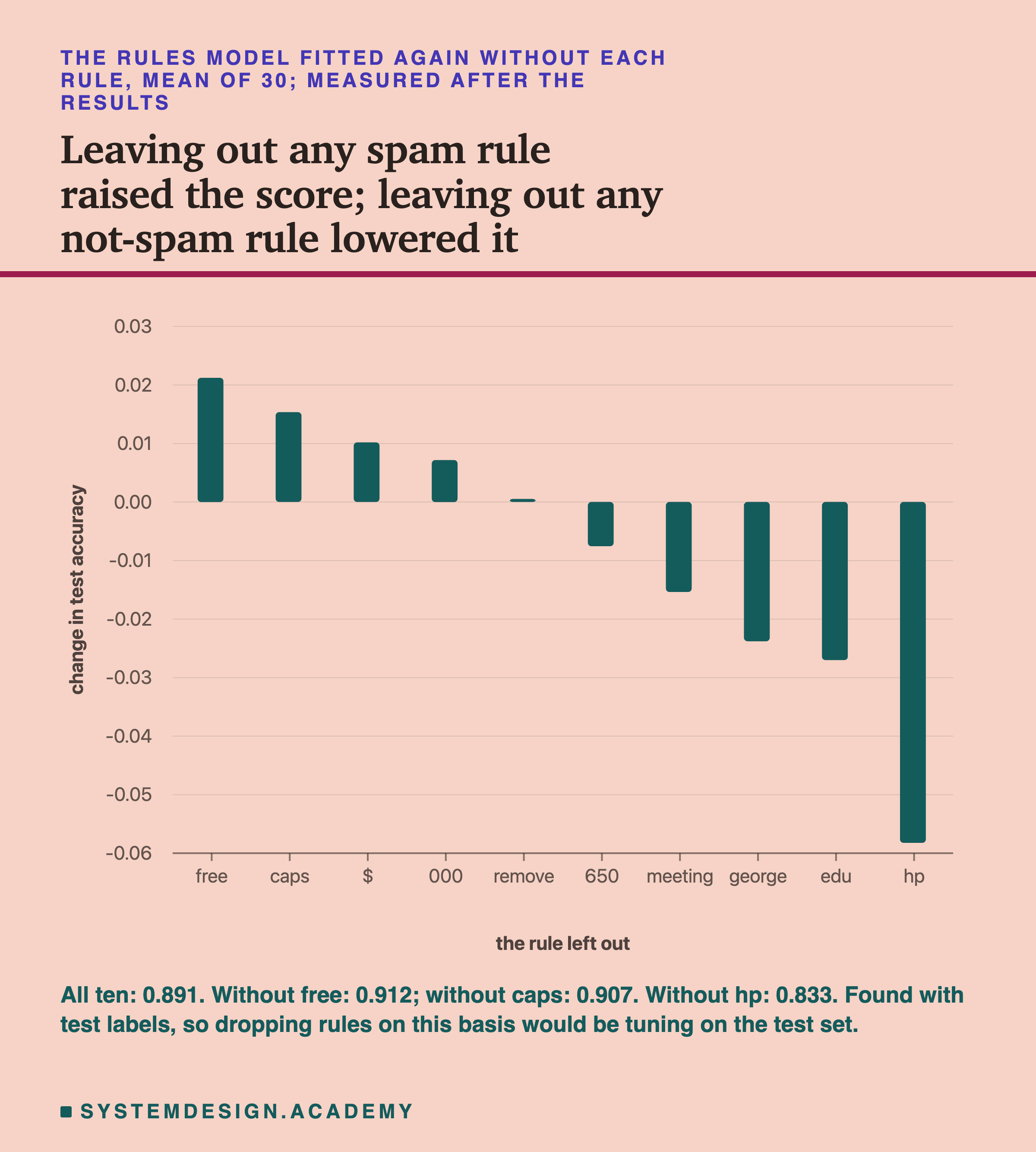
Write rules for what you already know. Check each one on a small hand-labelled sample, not on the test set. Here, ten rules with no labels scored 0.891. Leaving out any one spam rule raised the score, and leaving out any one not-spam rule lowered it.
Start active learning from random labels. Buy a small seed set first, the first labels bought at random, then buy the unsure ones in rounds, fitting the model again between rounds.
Compare it with random on the same budget before you trust it. Here, at 50 labels, the aimed labels were behind in 21 of 30 repeats. From 200 labels they were ahead in 29 or 30.
Relabel a fresh sample when a label's meaning changes. Schedule it, like retraining.
When to Aim the Labels, and When Not To
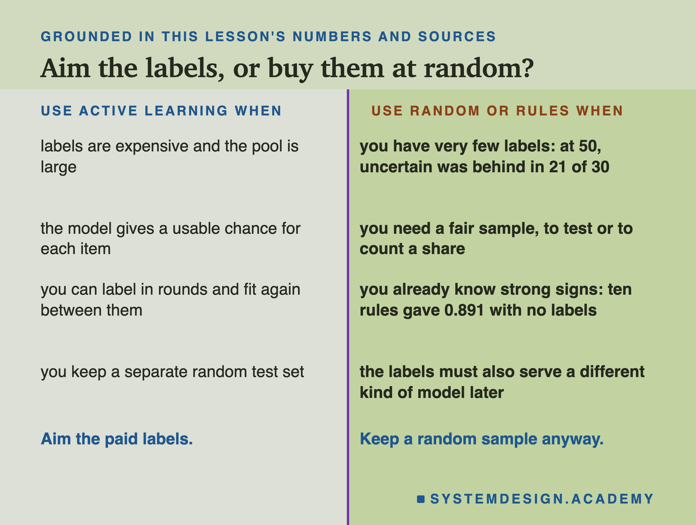
Use active learning when labels are expensive and the pool is large. Here it matched the full pool's accuracy with 500 of 3,450 labels. With cheap labels or a small pool, the saving may not be worth the rounds.
Use it when the model gives a usable chance for each item, and you can label in rounds. Uncertainty sampling needs a score to sort by, and it needs to fit the model again between rounds, so the labellers and the model have to take turns.
Use it only with a separate random test set. The labels it buys are the hard ones, so they cannot tell you how good the model is.
Buy at random when you have very few labels. Here, at 50 labels, random was ahead in 21 of 30 repeats. A seed set of random labels helps, but expect a slow start anyway: this lab began with a seed set of 20 and was still behind at 50.
Buy at random when you need a fair sample, to estimate how common something is or to test a model. Uncertain's labels were 48.6 percent spam where the pool was 39.4.
Use rules when you already know strong signs. Ten rules gave 0.891 with no labels here. Check each rule on a small labelled sample, and expect some to hurt.
Be careful when the labels must serve a different model later. Settles's survey warns that a set built by active learning is "inherently tied to the model that was used to generate it". A set bought at random has no such tie.
Common Mistakes When Buying Labels
Measuring the model on the labels active learning bought. They are the hard cases on purpose. Here a model scored 0.698 on them and 0.922 on a random test set.
Judging a strategy on one run. At 20 labels, two repeats of the same lab scored 0.706 and 0.903. At 100 labels, a mean advantage of 0.013 split 17 repeats to 13.
Starting active learning with almost nothing. A model with 20 labels is a poor judge of what is confusing. Start from a seed set of random labels and expect a slow first stretch.
Choosing rules by their test-set score. That turns the test set into training data. Here, dropping "free" raised the test score from 0.891 to 0.912, and I did not drop it for that reason.
Using rules that only work on one inbox. "george" was right 99.0 percent of the time because this dataset's normal emails were its donors' filed work and personal email. The dataset's own page says so.
Accepting model suggestions without a check. Keep hidden test items under the checking step, or a person clicking accept becomes the model with a person's name.
Labelling into a spreadsheet. A labelling tool keeps who labelled what, when, and how long it took. Label Studio's export has all three.
What I Corrected on This Page
This page replaced an older version of the same lesson. I checked every claim in the old version against its source, and these are the ones that did not hold. The full list, with each source and quote, is in scripts/labs/dataeng/results/lbg-factcheck.json.
-
"15 percent wrong labels cannot be saved by any tuning." Lesson 11 measured otherwise for random mistakes, so I took it out.
-
"Snorkel's label model learns how the rules are correlated." Its current documentation says it treats them as independent given the true label. Fixed here and in the diagram on the weak-supervision slide.
-
"Teams routinely need 2 to 10 times fewer labels with active learning." I found no source for that range, so I cut it and measured one case instead.
-
A table of prices per label for experts, vendors and crowds. I found no source for any of the ranges, so I cut it and showed Mechanical Turk's real fee rules instead.
-
"5x to 50x cheaper", "a transcript takes four times the clip" and "30 seconds to label, 10 to verify". No source found; cut.
-
A story about Tesla moving from large labelling teams to auto-labelling. I found only press reports of a 2021 talk, not the company's own words, so I cut it.
-
"Armies of human annotators" behind chat models. The InstructGPT paper names about 40 contractors, so I cut the phrase.
What These Numbers Can and Cannot Tell You
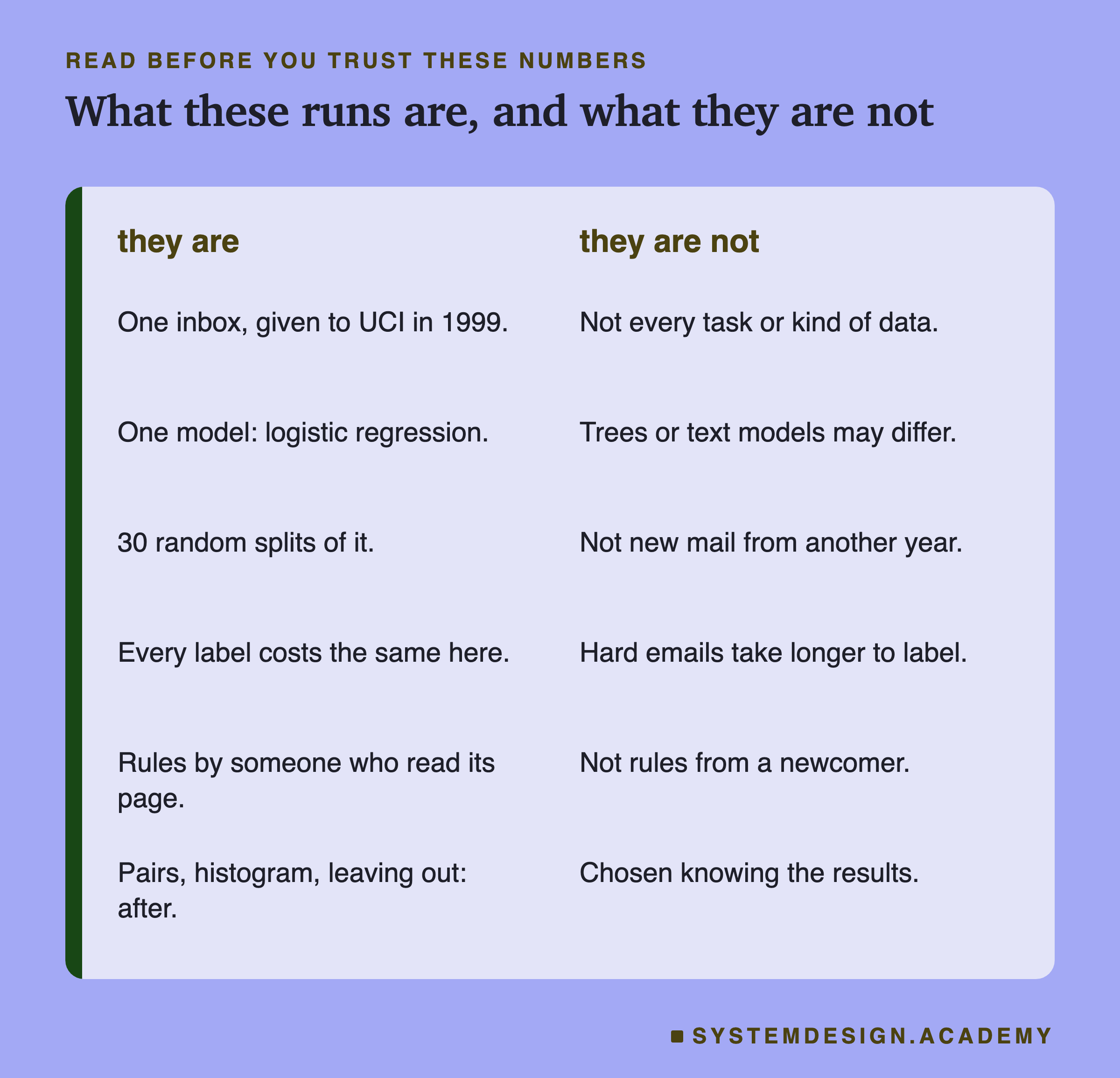
One inbox. Everything here is one collection of 4,601 emails, given to UCI in 1999, whose normal mail came from its donors' own work and personal email. Other data, other tasks and a newer inbox could give very different numbers.
One model. Logistic regression on 57 counts. A tree model, or a model that reads the raw text, could gain more or less from aimed labels.
Thirty random splits of the same emails. The repeats test how much the result depends on which emails land in the pool and the test set. They do not test new emails from another year.
Every label costs the same here. In real work the emails near 0.5 are likely to take longer to label. Settles's survey notes that "simply reducing the number of labeled instances does not necessarily guarantee a reduction in overall labeling cost". If your tool records time per item, as Label Studio's lead_time does, measure it.
Rules by someone who has read about the dataset. My ten rules were written before the first run, but not by a newcomer, and three of them rely on the dataset's own note about its donors.
Some parts came after the results. The design, the four ways, the rules, the budgets and the target were fixed before the first run. The paired counts, the look inside repeat 0, the typical-email test and leaving rules out came after. I wrote them into the report's design before the report first ran. The worked email was added while I wrote the lesson.
What to Do Next
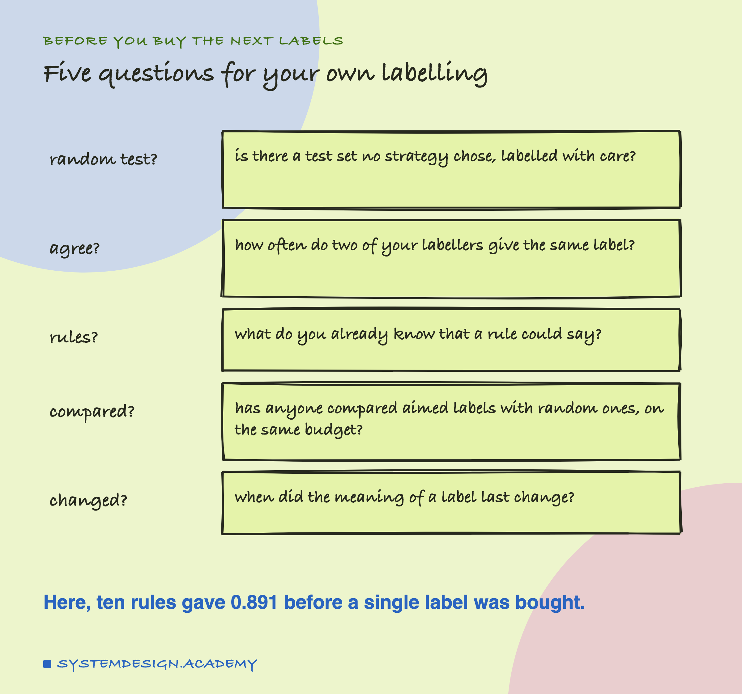
Take one labelling job your team runs and ask the five questions on the card. The first is the most important. Is there a test set that no strategy chose, labelled with care? If not, every number you have about your model might be measured on the wrong emails.
Then do the measurement. Take a pool you already have labels for, hide them, and replay random labelling against uncertainty sampling on the same budget, many times. Write a few rules and check them on a small labelled sample. Here, the aimed labels needed 188 on average to get within 0.01 of the full pool. Random did not get there by 500 in 18 of 30 repeats, and ten rules gave 0.891 for nothing. Your numbers will differ, and now you have a way to find them.
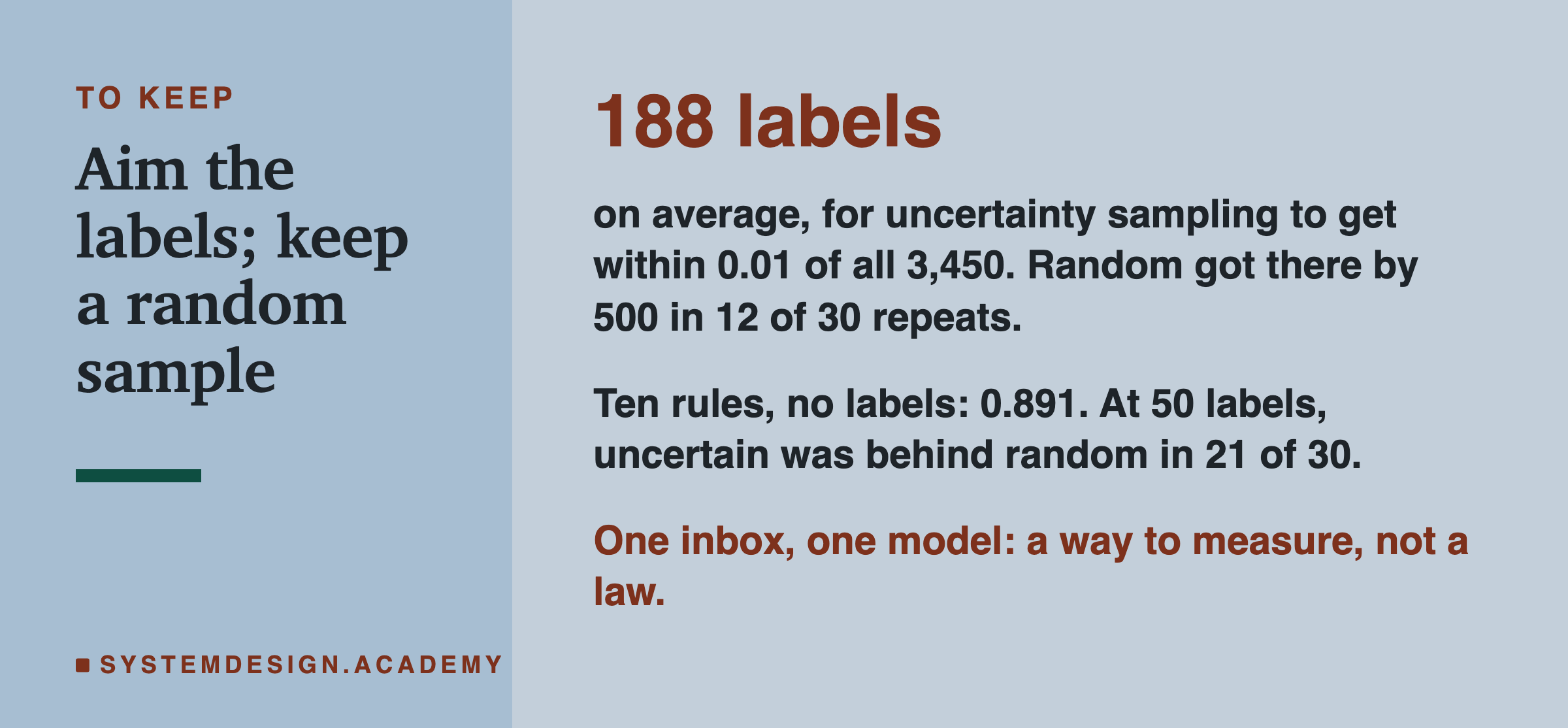
The card keeps the lesson's numbers. Uncertainty sampling needed 188 labels on average to get within 0.01 of all 3,450, and did so in every repeat. Random labelling got there by 500 labels in 12 of 30. Ten rules and no labels scored 0.891. At 50 labels, aiming was behind random in 21 of 30 repeats.
The next lesson in this chapter is about handling imbalanced data, for when one label is far rarer than the other.
Knowledge Check
Knowledge Check
4 questions - Score 80% to pass
In the lab, at 50 labels, how did uncertainty sampling do against random labelling on the same 30 splits?
Why does the lesson say never to measure a model on the labels active learning bought?
Leaving out the rule for 'free' raised the rules model from 0.891 to 0.912. What does the lesson say to do with that?
What does Snorkel's current LabelModel documentation say it assumes about the labelling rules?