Imagine a small cafe that has sold the same house coffee for years. A supplier offers a new blend. The owner does not want to change without a good reason, so she runs a taste test: ten regular customers try both cups without knowing which is which, and she will switch if more of them prefer the new one. Six of the ten pick the new blend. Does she switch?

Think about what the six really tells her. If the two blends tasted exactly the same, each customer would be picking at random, like tossing a coin. Six heads out of ten tosses happens all the time. So would five, and so would seven. Ten customers are simply too few to tell a real difference from chance.

There is a second, quieter point in her test. Some customers like both cups equally, or dislike both. They tell her nothing about which blend is better. Only the customers who clearly preferred one cup carry any information. If she has 100 customers and 90 of them cannot tell the cups apart, her decision really rests on the other 10. Asking the same people about both cups, and counting only those who preferred one, is called a paired test: both things are judged on the same cases.

This lesson is about the same decision for a program that learns from examples. A new version of the program wants to replace the one in use. I measured how often three ways of deciding let a new version through when it was no better, and how often they caught one that really was.

This chapter follows a model through its life, one step at a time, on the same data. Start with the dumbest model showed that a rule with no learning beat every trained model on the future. Same code, different model trained the same model 20 times, changing only the seed, and got 20 different models. Picking the best of many showed that the winner of a large search can do worse on later months than a setting picked at random.

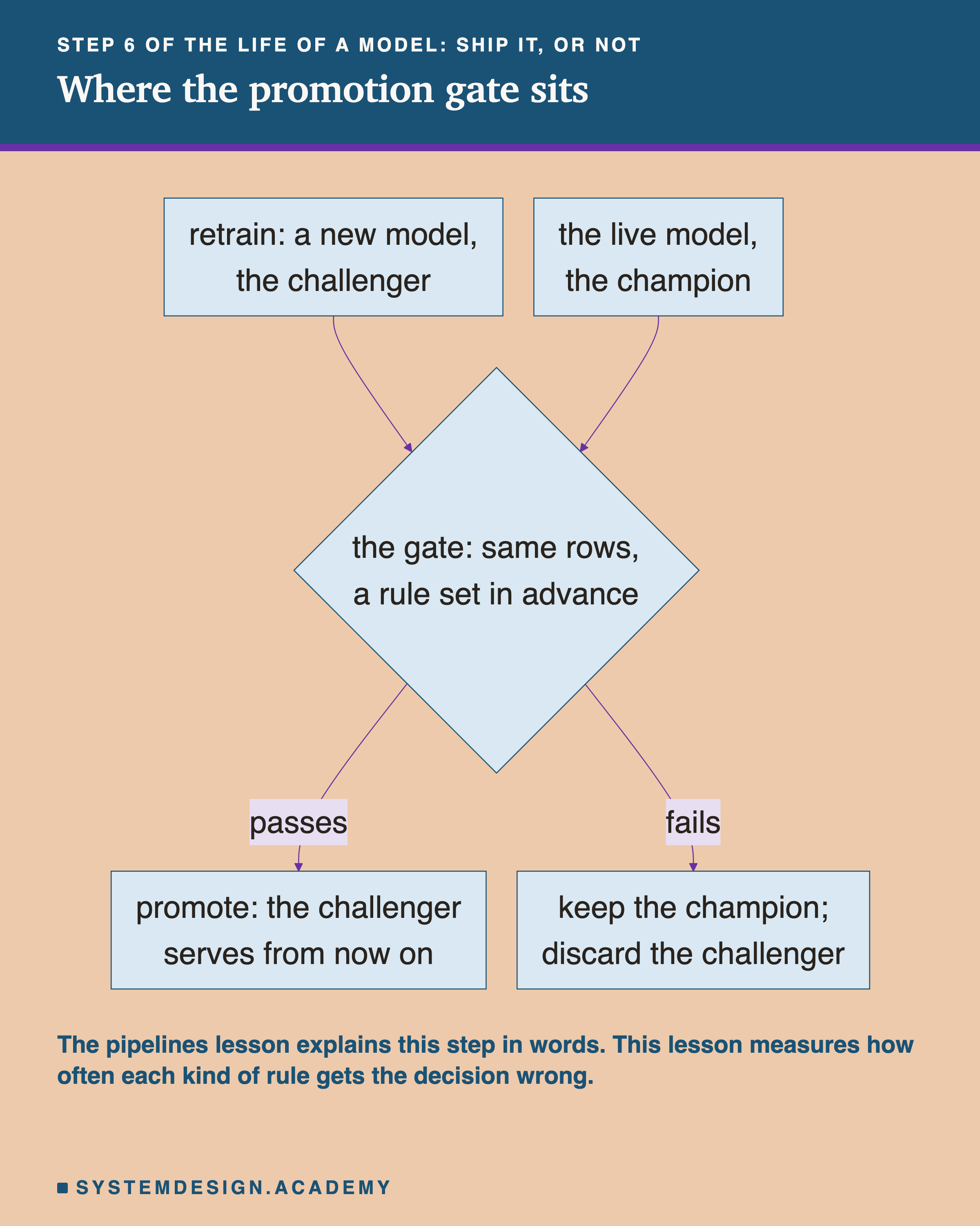
Now the model is trained, and the question is whether it should replace the one already running. The course's lesson on training pipelines and orchestration has a slide called "The Gate: When to Ship, When to Hold". It explains, in words, the idea of a gate that compares the new model with the live one on held-out rows (rows neither model learned from), and a margin set in advance. I will not repeat it. This lesson measures how well such a gate works.

Lesson 2 matters most here. A seed is the starting number for a model's random choices; scikit-learn calls it random_state. Lesson 2 found that two seeds of the same code give two genuinely different models, sometimes several points apart. So a pipeline that retrains on a schedule produces a new, different model every time, even when nothing about the data or the code changed. Each of those models arrives at the gate. The gate is what decides whether that difference is progress or luck.

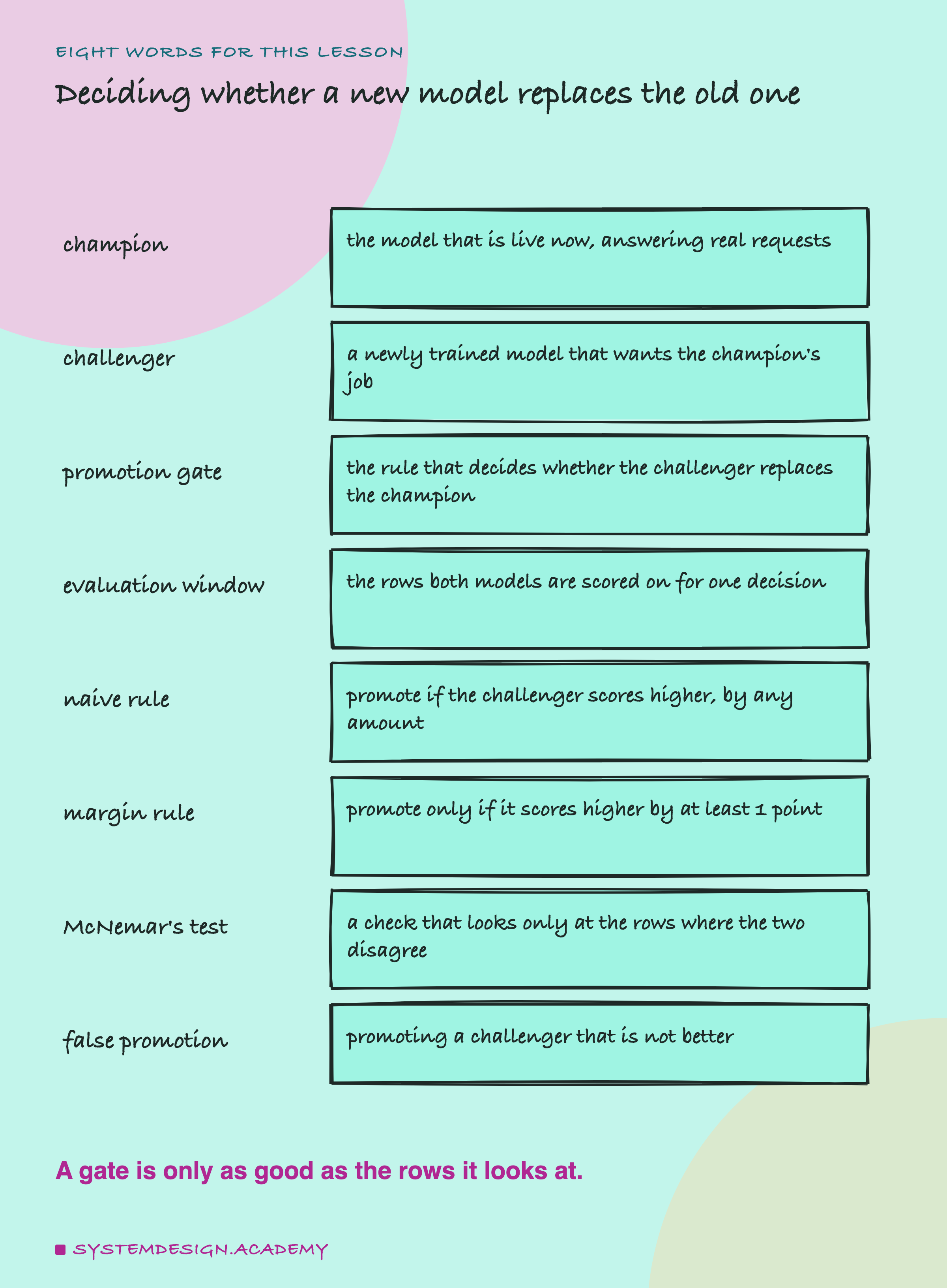
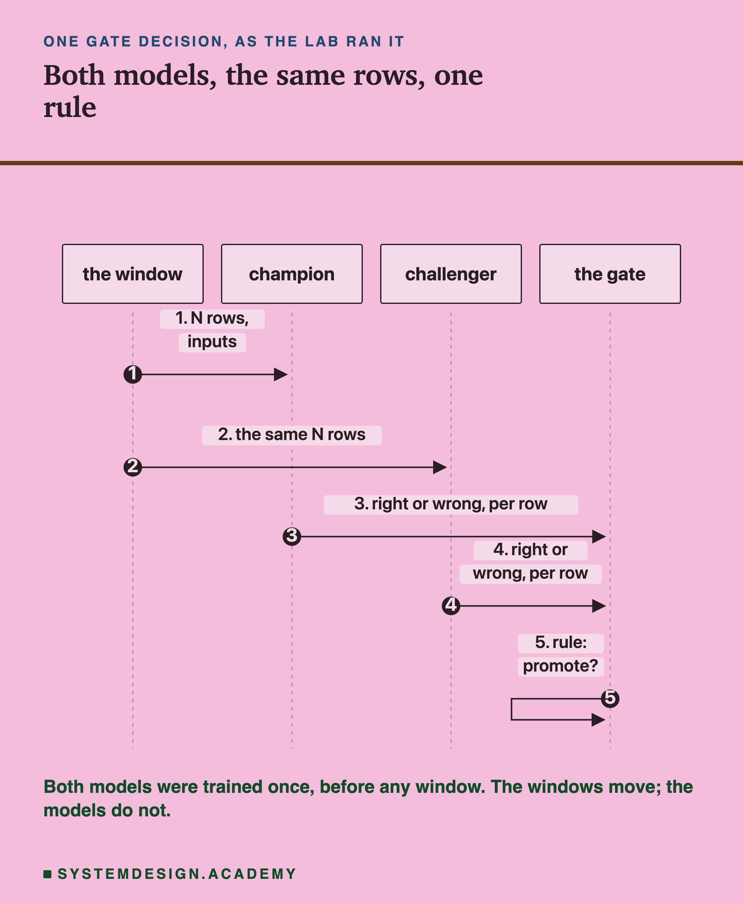
The champion is the model that is live now, answering real requests. The challenger is a newly trained model that wants the champion's job. The promotion gate is the rule that decides whether the challenger replaces the champion. To promote a model is to put it live in place of the old one.

The gate scores both models on the same rows. I call one such set of rows an evaluation window, and N is the number of rows in it. Accuracy is the share of rows a model got right, and a point is one hundredth of accuracy.

The naive rule promotes the challenger if it scores higher, by any amount. The margin rule promotes it only if it is ahead by a fixed amount, here 1 point. McNemar's test is a check that looks only at the rows where the two models disagree; the next slides explain it. A false promotion is promoting a challenger that is not better. A null, in this lesson, means a pair of models where neither is better, so any promotion is a false one. A paired comparison scores both models on the same rows and compares them row by row, which is what all three rules here do.

All three rules look at the same thing: two models, scored on the same window of rows, each row marked right or wrong for each model. They differ only in what they demand before they say yes.

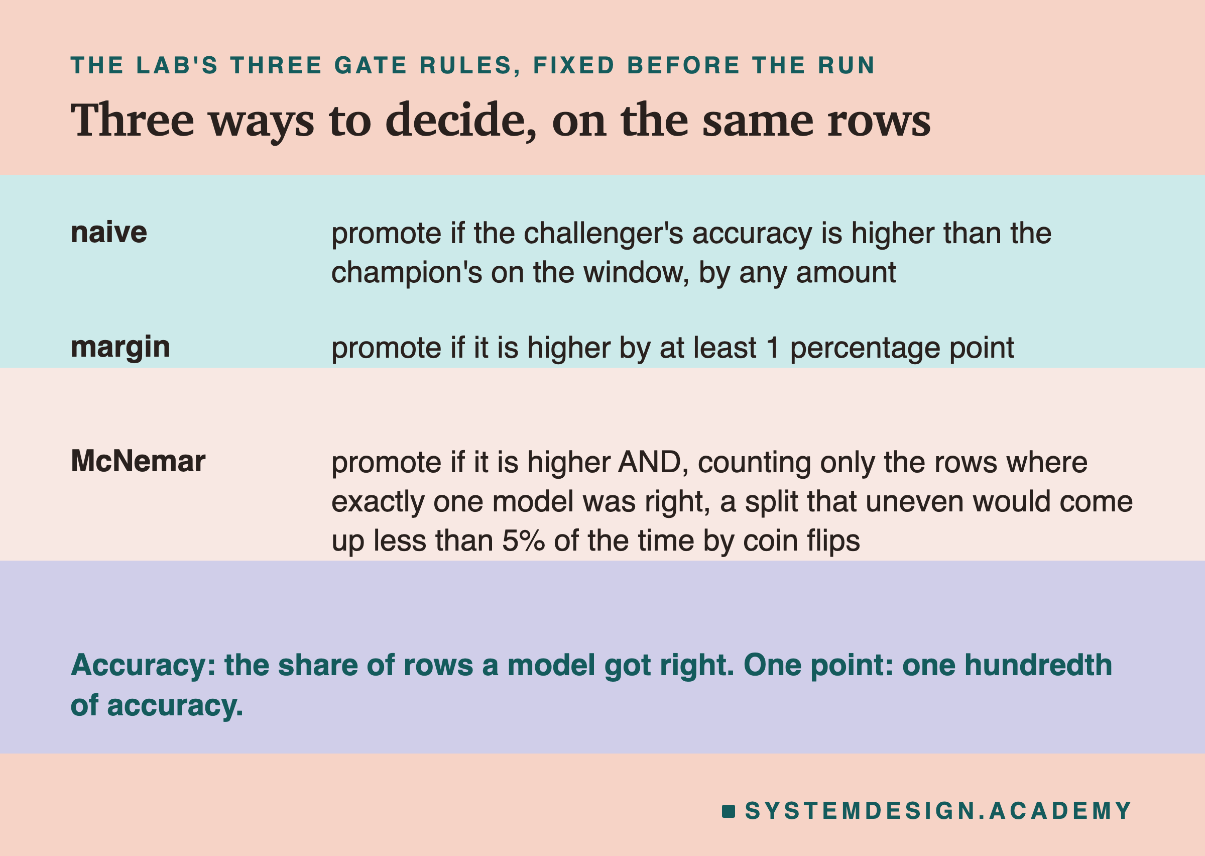
Naive. Higher wins. If the challenger got 158 of 200 rows right and the champion 157, the challenger is promoted. This is what a pipeline does when someone writes "if new score is greater than old score, deploy". It is a rule I have often seen in pipelines, because it is the first one anyone writes.

Margin. The challenger must be ahead by at least 1 point: on 200 rows, that is at least 2 more rows right. This is the rule the pipelines lesson describes, with a margin set in advance. The idea is sound: demand a little more than zero, so that tiny, lucky leads do not get through. The question this lesson asks is whether a fixed margin is enough, and the answer depends on the size of the window.

McNemar. The challenger must be ahead, and the lead must pass a test that asks: if the two models were equally good, how surprising would a split this uneven be? The test reads only the rows where the two models disagree. If that surprise is large enough, meaning such a split would happen less than 5% of the time between two equal models, the challenger is promoted.

All three rules were fixed in the lab file before it ran. None was tuned after I saw the results.

McNemar's test is named after the psychologist Quinn McNemar, who published it in 1947; this lesson uses its exact form, which counts coin tosses directly. It is built for exactly this situation: the same cases, judged twice, each time right or wrong. Here the cases are rows and the two judges are two models.

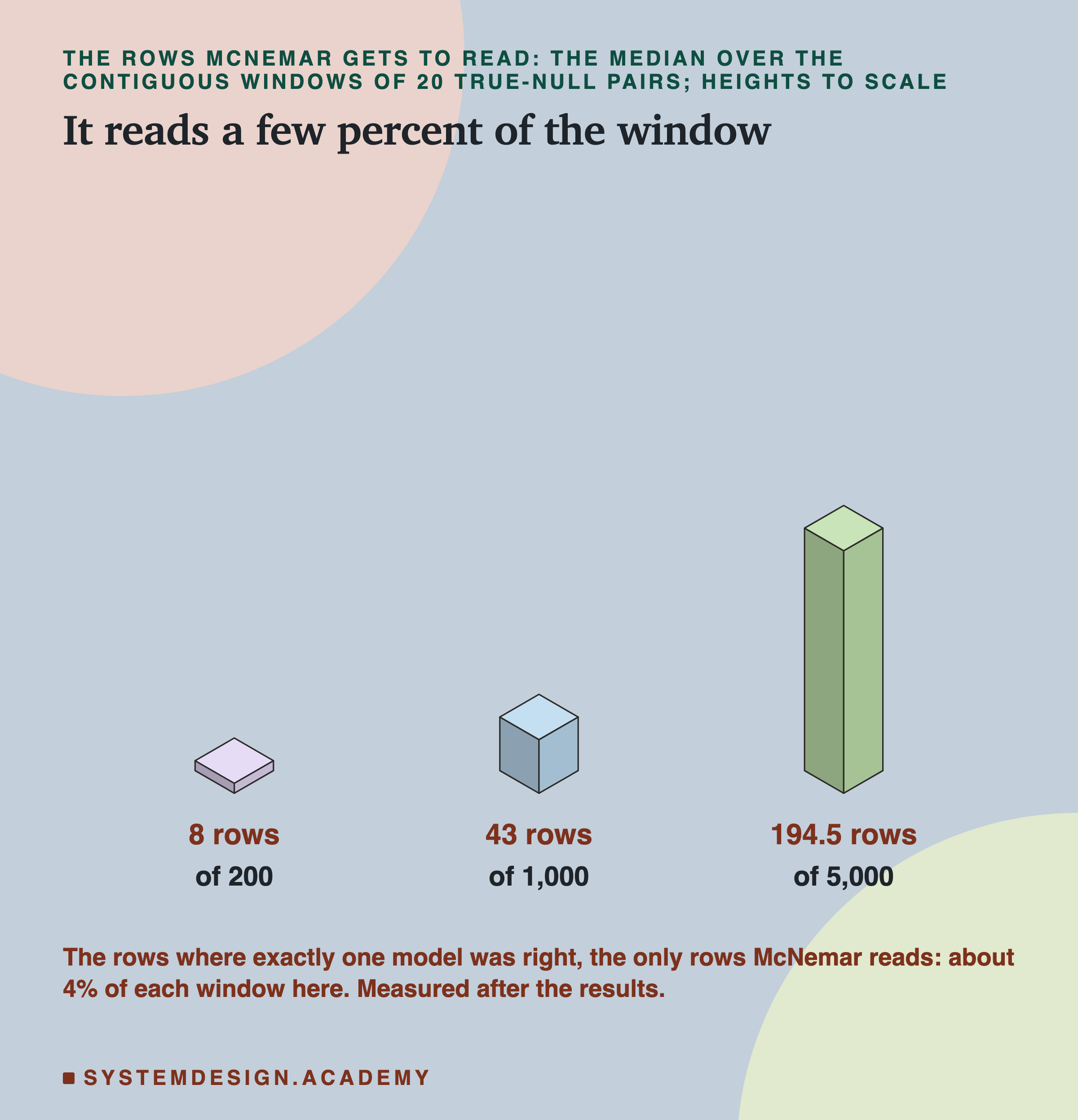
Put every row of a window into one of four boxes. Both models right. Both models wrong. Only the challenger right. Only the champion right. The first two boxes say nothing about which model is better: on those rows the two behaved the same. Only the last two boxes can tell them apart, just like the cafe customers who clearly preferred one cup.

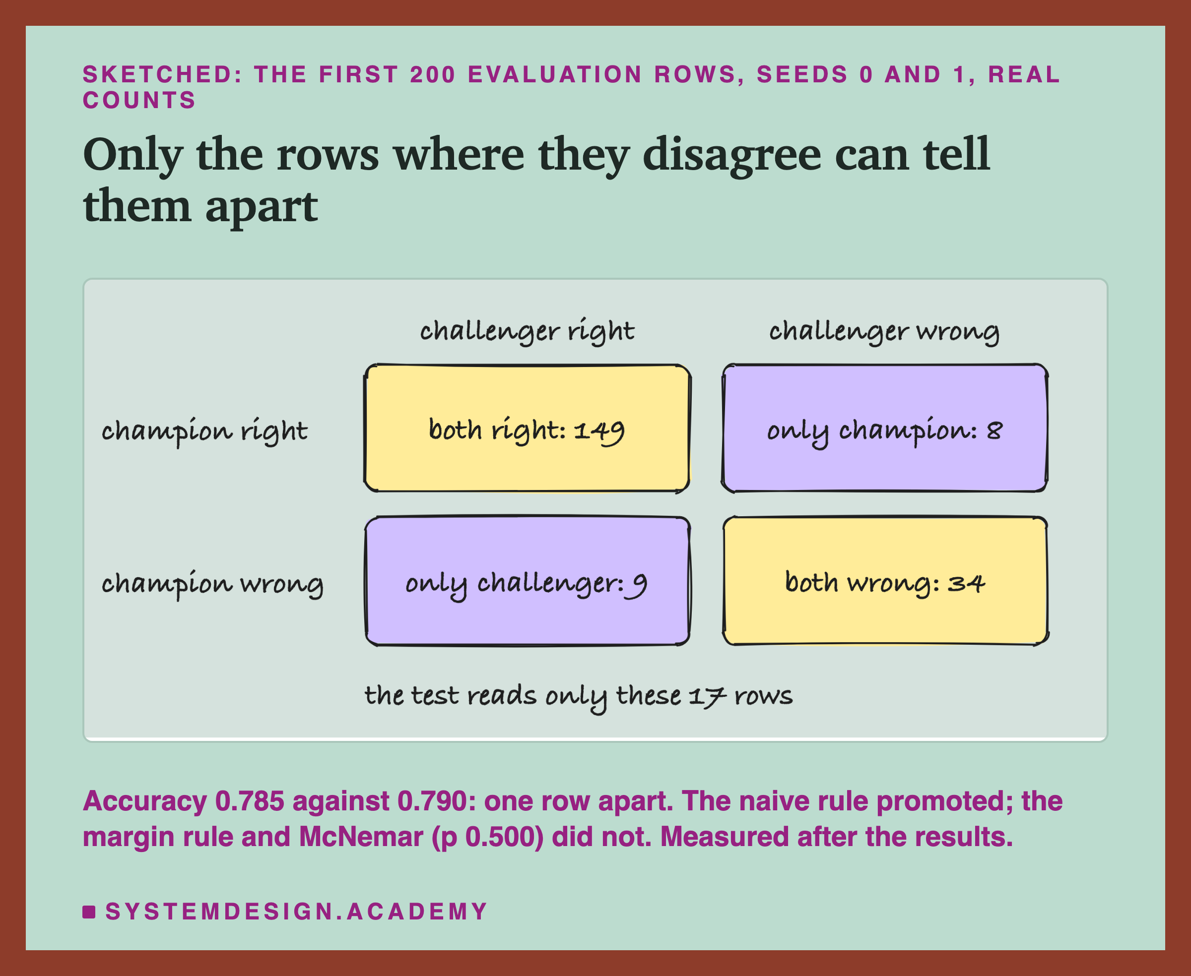
This is a real window: the first 200 evaluation rows, with the trees trained with seed 0 as the champion and seed 1 as the challenger. They were both right on 149 rows and both wrong on 34. On 17 rows they disagreed: the challenger alone was right on 9, the champion alone on 8. So the challenger scored 0.790 and the champion 0.785, one row apart, and the naive rule promoted it.

Now the test. Suppose the two models were equally good. Then each of the 17 disagreeing rows is like a coin toss: as likely to go to one model as the other. The test asks how often 17 fair coin tosses give 9 or more heads. The answer, called the p-value, is 0.500: half the time. Nothing surprising at all, so McNemar said no.

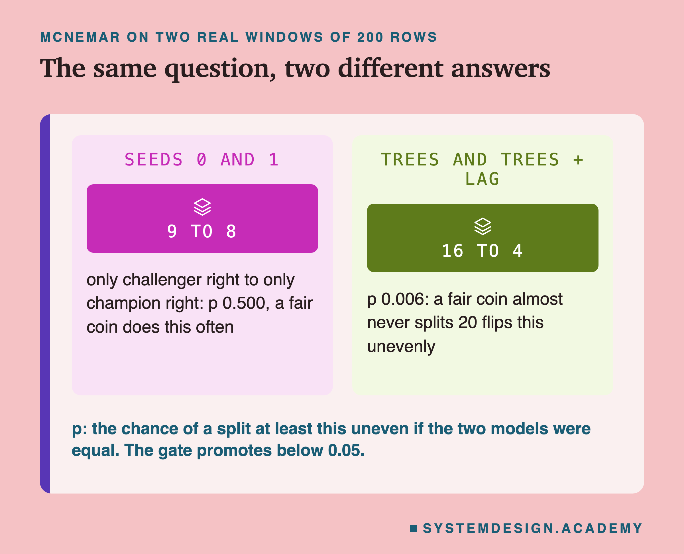
The second panel is the same first window for a pair where the challenger really is better: the trees with the previous half-hour's label as an extra input, from lesson 1. There the two disagreed on 20 rows, and the challenger was right on 16 of them. Sixteen or more heads in 20 fair tosses happens with a chance of 0.006, so McNemar said yes.

I wrote the lab's design at the top of its file, gate_lab.py, before it ran. The dated record is in the chapter plan (2026-09-29, "GATE LAB (batch 4) designed before running").

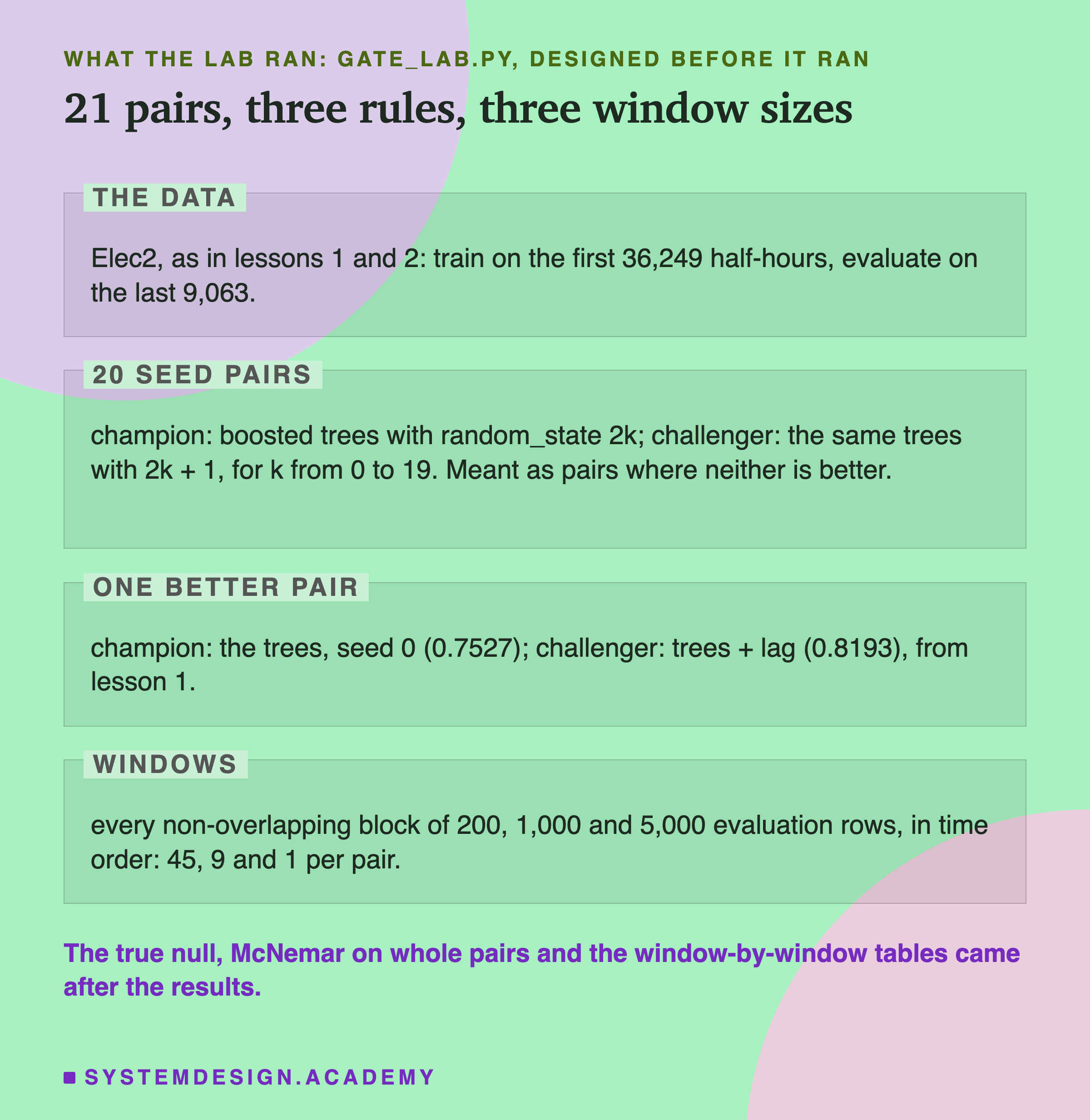
The data is Elec2 again: 45,312 half-hours of the New South Wales electricity market in time order, where each row asks whether the price is UP or DOWN against its average over the last 24 hours. Every model trains on the first 36,249 rows and is evaluated on the last 9,063.

The pairs. Twenty seed pairs: the same boosted trees trained with seeds 0 and 1, 2 and 3, and so on up to 38 and 39. The design called them null pairs, meant as pairs where neither model is better. The next slides show that this was wrong, and why. One better pair: the plain trees as champion against the trees plus lag as challenger, 0.7527 against 0.8193 on the whole evaluation, a gain of 6.7 points.

The windows. A real gate usually sees the most recent rows, so the lab cut the evaluation into contiguous blocks of N rows, meaning rows that sit back to back in time with no gaps, and with no overlap, for N of 200, 1,000 and 5,000. That gives 45 windows of 200 per pair, 9 of 1,000, and just 1 of 5,000. For every pair, rule and N, the lab stored the share of windows in which the challenger was promoted.

Here is what the lab stored, in results/gate.json.

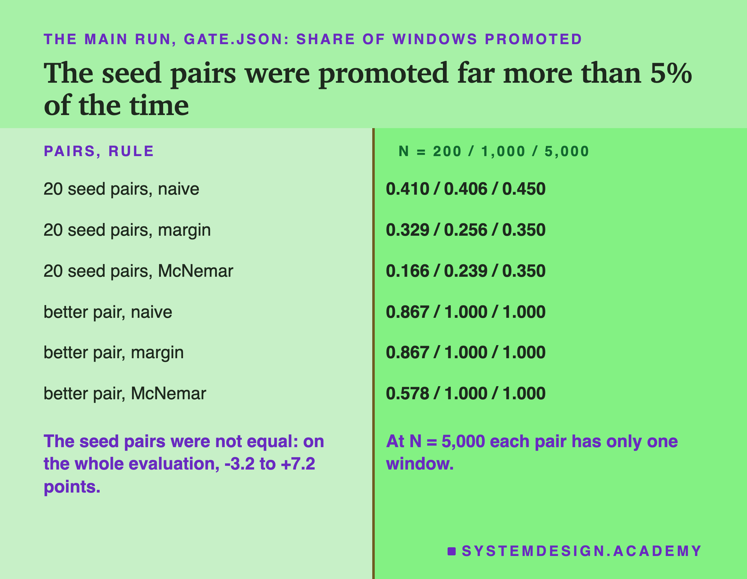
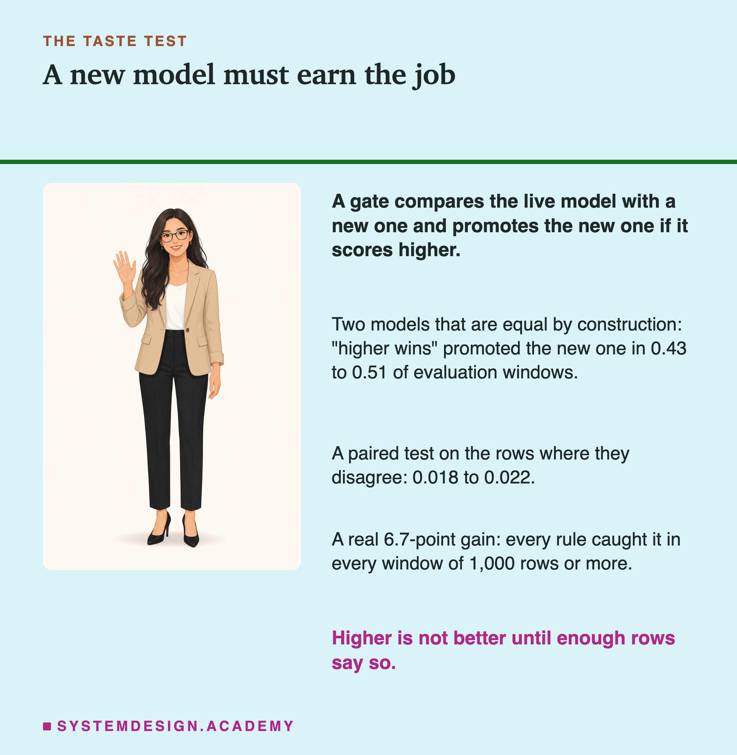
For the seed pairs, the naive rule promoted the challenger in 0.41 to 0.45 of the windows, depending on N. That part was expected. The surprise was McNemar: 0.17 of windows at N = 200, 0.24 at 1,000, and 0.35 at 5,000. If these pairs were truly equal, McNemar should promote in about 5% of windows or fewer. It was promoting three to seven times as often, and more often with bigger windows, which is the wrong direction for a test that is merely noisy.

The better pair looked as it should. Every rule promoted it in every window of 1,000 and 5,000 rows. With 200 rows, naive and margin promoted it in 0.867 of windows and McNemar in 0.578.

Before reading anything into the seed pairs' numbers, I checked the pairs themselves. On the whole evaluation of 9,063 rows, the challenger minus the champion ranged from -3.2 to +7.2 points. Those are not equal models. So the main run's "false promotions" are a mix of two things: gate errors, and real differences between two seeds that the gate correctly noticed. The main run cannot separate the two, and I will not quote its McNemar numbers as false-promotion rates.

This is lesson 2's finding, now showing up at the gate. Lesson 2 found that the default boosted trees hold back a random tenth of the training rows, chosen by the seed, so each seed trains on a different 90% of the data. The models that come out differ, sometimes by several points.

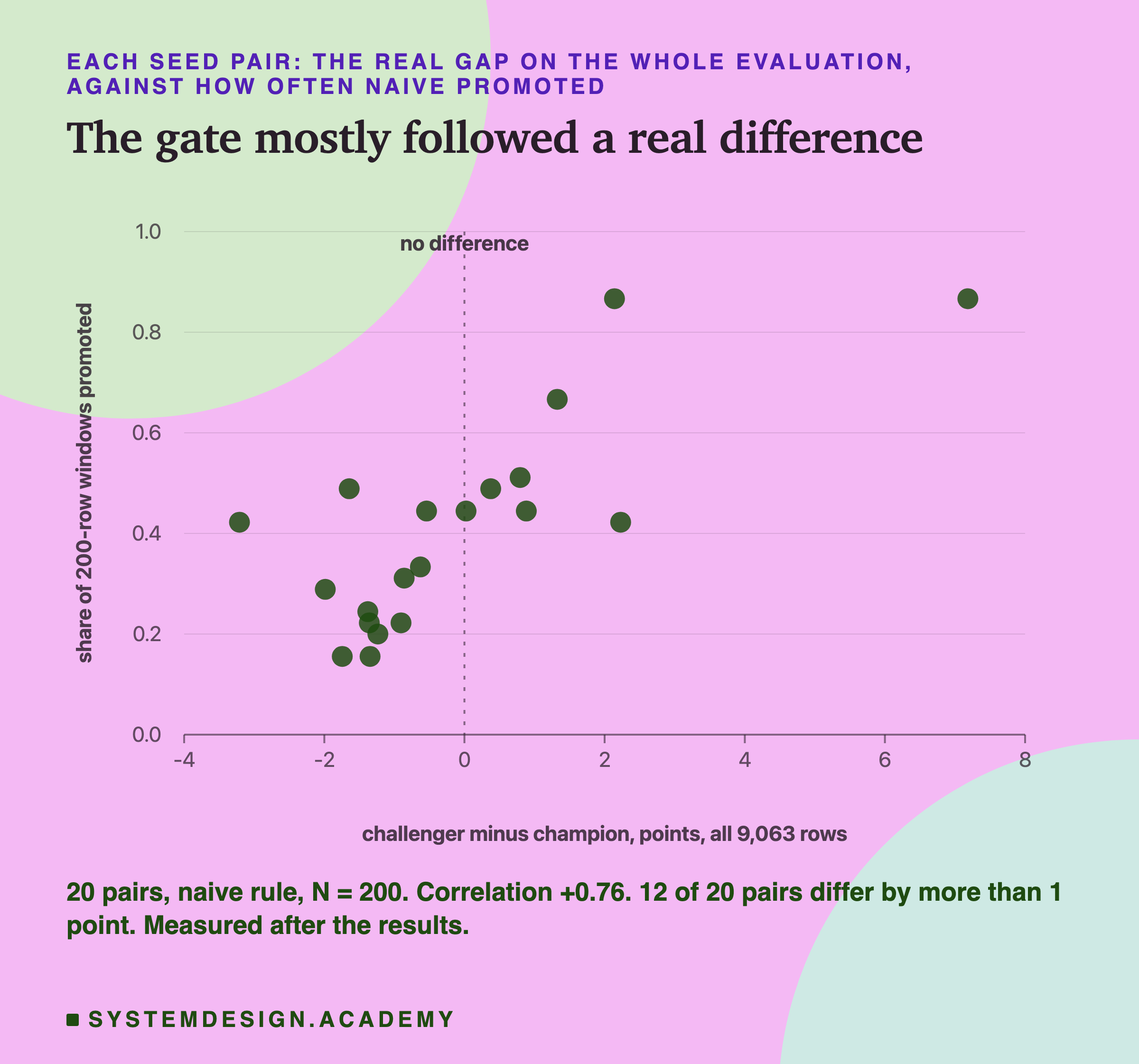
After the results, I plotted each seed pair's real gap on the whole evaluation against how often the naive rule promoted its challenger in 200-row windows. The two go together: the correlation, a number from -1 to 1 that measures how closely two things rise together, is +0.76. Pairs where the challenger really was better got promoted more; pairs where it was worse got promoted less. 12 of the 20 pairs differed by more than 1 point on the whole evaluation.

Then I ran McNemar's test on each pair's whole evaluation, all 9,063 rows, in both directions.

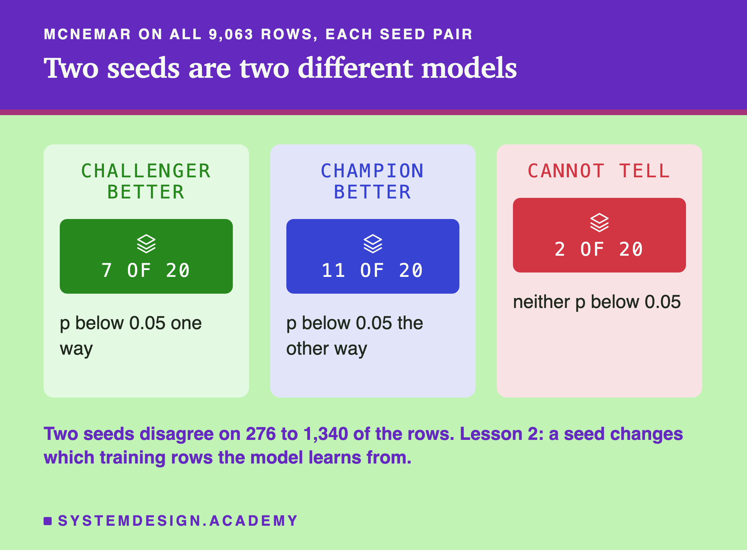
In 7 of the 20 pairs the challenger was clearly better, in 11 the champion was, and only in 2 could the two not be told apart. Two seeds disagreed on 276 to 1,340 of the 9,063 rows. So on this data, a retrain with a new seed is not "the same model again". It is a different model, and most of the time a measurably better or worse one.

That changes what the main run's McNemar numbers mean. With 5,000 rows, each pair had one window covering more than half of the evaluation. McNemar promoted 7 challengers there, and 6 of those 7 were among the 7 that were clearly better on the whole evaluation. That is mostly not a false promotion. It is an honest answer to a question the design got wrong: these were never null pairs.

For a team, the lesson is practical. A scheduled retrain can make the model worse, by several points, with no change anyone made. The gate is the only thing between that model and your users. To measure how often a gate is fooled, I needed pairs that were truly equal.

I designed a follow-up after I saw the main results, and wrote its design into the lab file's followup mode before it ran. Its results are in results/gate_followup.json.

The idea is a way to build two models that are equal by construction. Take each seed pair. On every evaluation row, toss a coin. On heads, swap the two models' outcomes on that row: the champion gets the challenger's right-or-wrong, and the challenger gets the champion's. On tails, leave the row alone. After the swap, on every single row, each of the two "models" has the same chance of having the better outcome. Neither can be better by design, so any promotion is a false one.

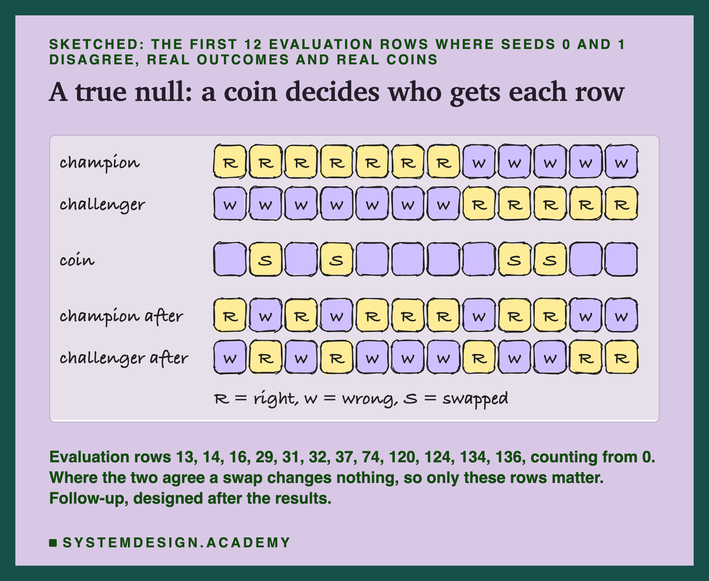
The sketch shows the first 12 evaluation rows where seeds 0 and 1 disagree, with their real outcomes and the real coin tosses. Where the two models agree, a swap changes nothing. Where they disagree, the coin decides which model gets the right answer. The disagreeing rows are exactly the ones McNemar reads, so this builds what McNemar's test assumes: that each disagreeing row is a fair coin.

The follow-up did this for all 20 seed pairs, with one fixed seed for the coins, and ran the same three rules on the same contiguous windows as the main run.

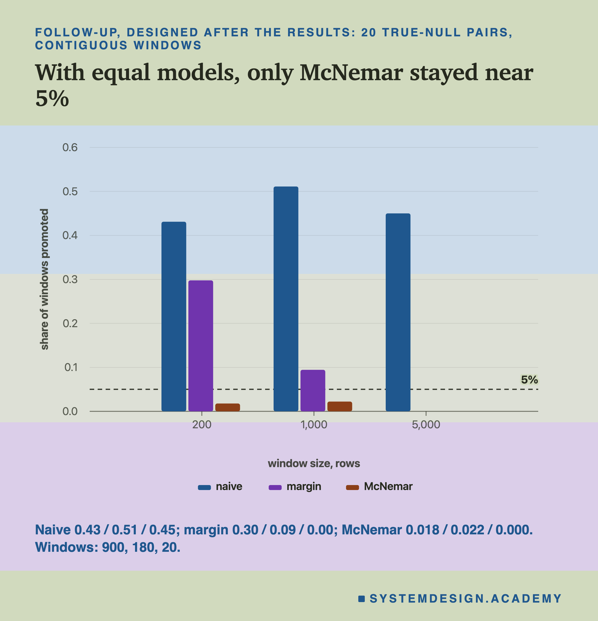
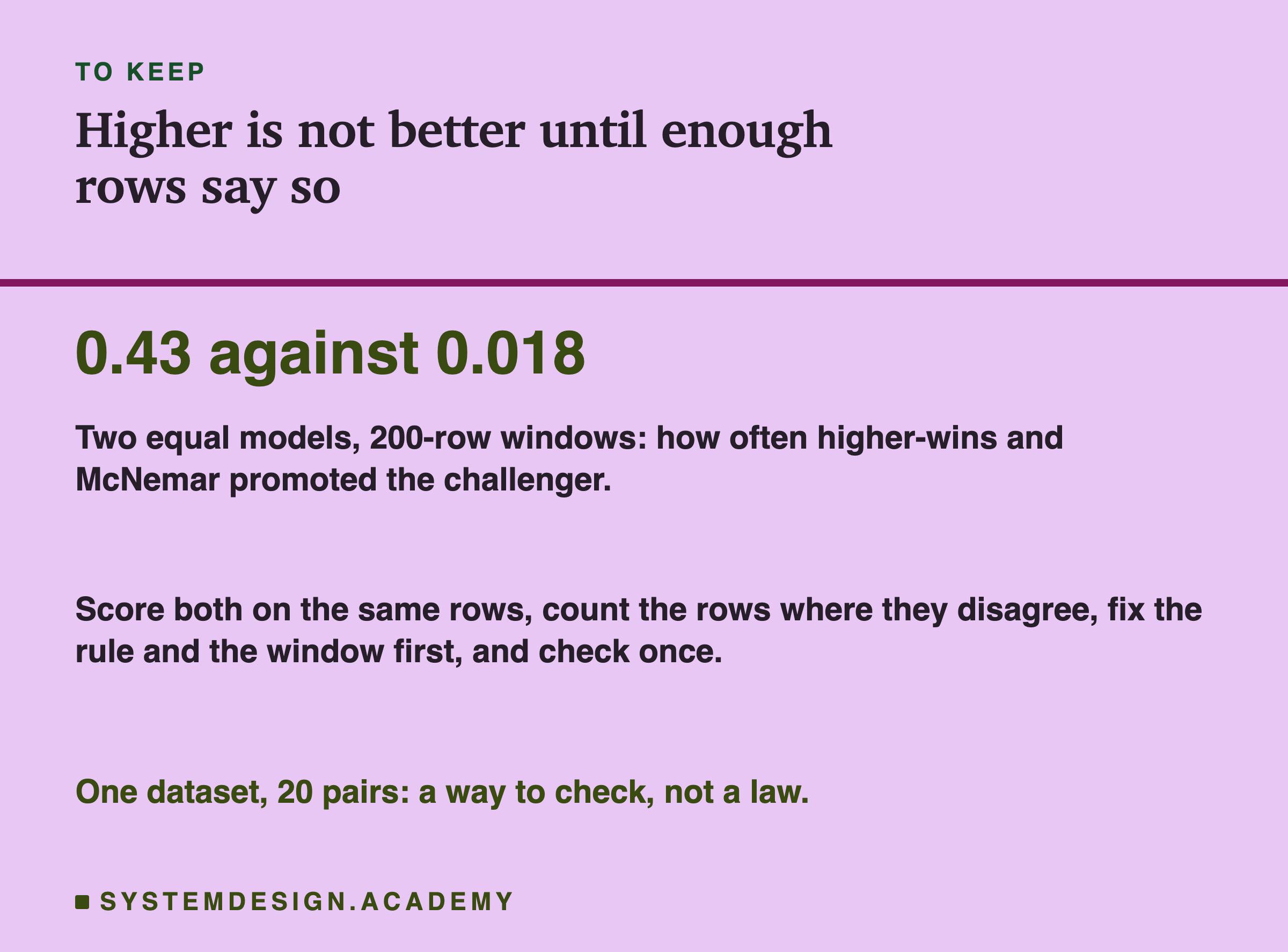
The naive rule's result has a simple cause. When two models are equally good, which one scores higher on a given window is decided by the luck of the rows in it. It is a coin flip, and a coin flip lands heads about half the time. That is exactly what "higher wins" did: it promoted an equal challenger in 0.43 to 0.51 of contiguous windows, whatever the size.

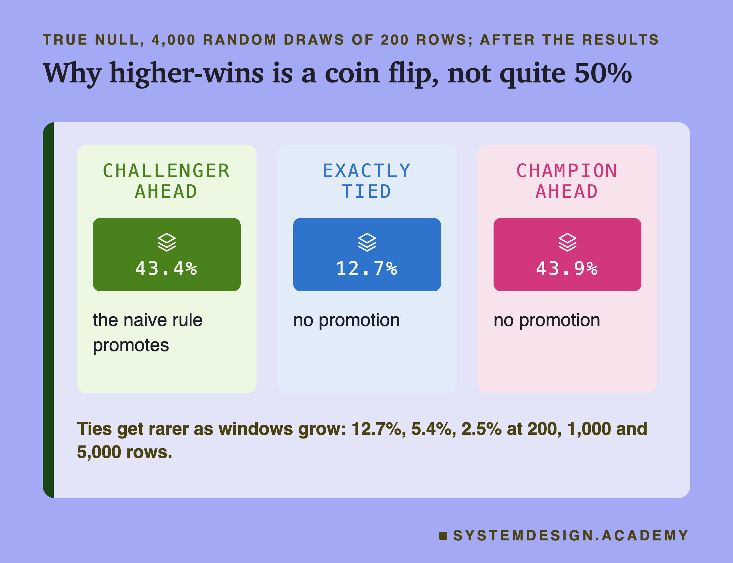
Why is it a little under half at 200 rows? Because of ties, which I counted on the follow-up's random draws. In 12.7% of 200-row draws the two equal models got exactly the same number of rows right, and a tie is not a promotion. The challenger was ahead in 43.4%, the champion in 43.9%. As windows grow, ties get rarer: 5.4% at 1,000 rows and 2.5% at 5,000. So the naive rule sits near 50% at every size. Bigger windows do not help it at all.

That is the key point about the naive rule. It does not become safer with more data. With 200 rows or 5,000, it promotes an equal model about half the time. A pipeline that retrains every week with this rule would, over a year, swap its model many times for no reason, and each swap is a new model with its own new mistakes that someone may have to debug.

It also means the naive rule cannot tell a small real gain from luck. If the challenger is really a little better, it will be ahead in somewhat more than half of windows, and behind in the rest. The rule gives no warning which case you are in.

The margin rule is the naive rule with a hurdle: be ahead by at least 1 point. It helped a great deal at 1,000 rows (0.09) and at 5,000 (0 of 20 contiguous windows, 0.02 of random draws), but not much at 200 (0.30). Why the difference?

Because a point is a different thing at each size. On 200 rows, 1 point is 2 rows. On 1,000 rows, it is 10 rows. On 5,000 rows, 50. And the luck of the rows moves the gap between two equal models by an amount that shrinks as the window grows.

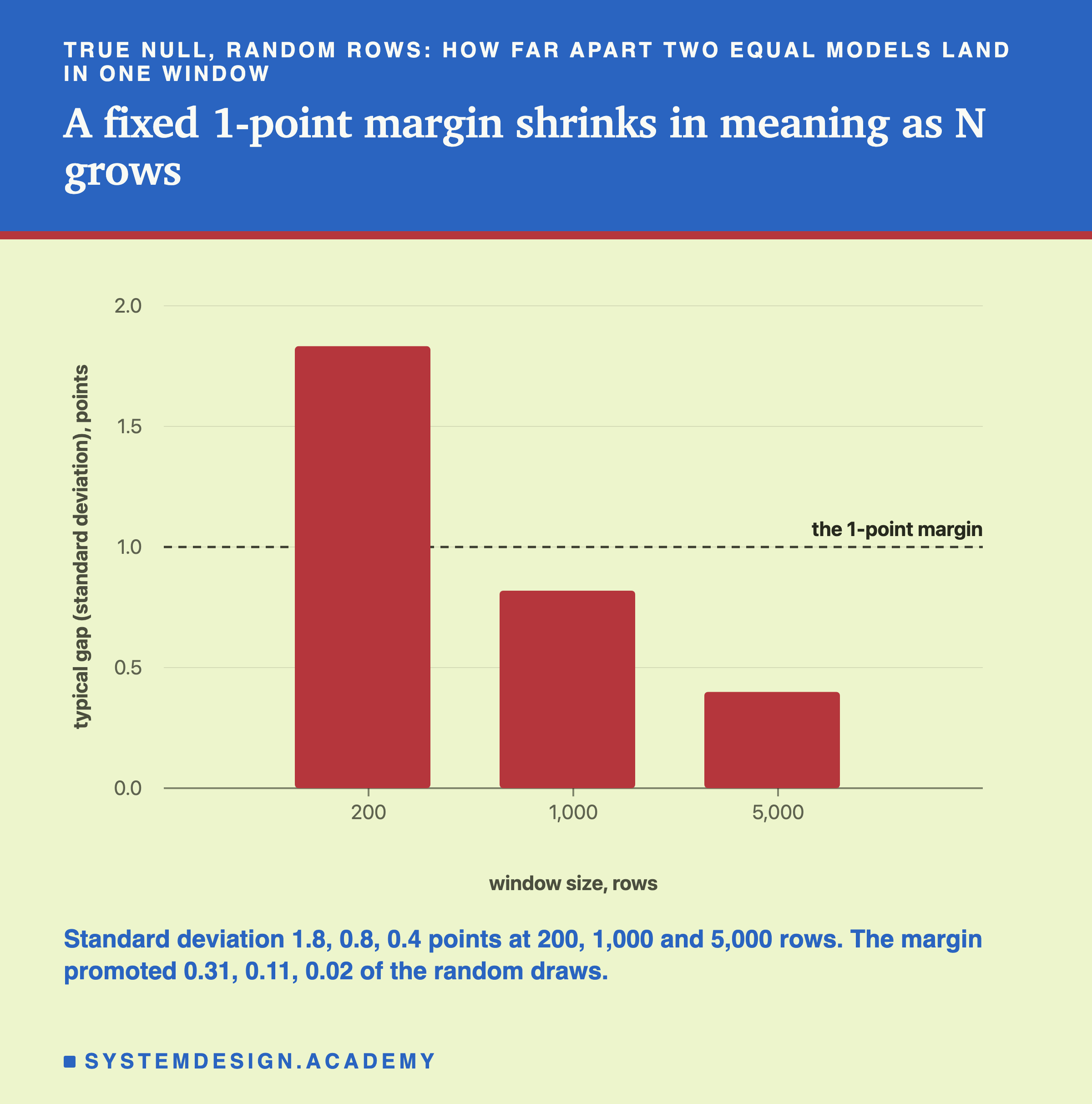
I measured that spread on the follow-up's random draws of equal models. The standard deviation, a measure of how far values typically land from their average, was 1.83 points at 200 rows, 0.82 at 1,000 and 0.40 at 5,000. So with 200 rows, two equal models typically land almost 2 points apart, and a 1-point hurdle is easily cleared by luck. With 5,000 rows they typically land less than half a point apart, and 1 point is rarely reached.

A fixed margin, then, means something different at every window size. It is not wrong; it is just not self-adjusting. If you set a margin, you have to choose it for the size of your window. A margin sized to stop luck at 200 rows, one that two equal models cross only about one time in twenty, is 1.645 × 1.83 = 3.01 points: 7 rows on 200, since part of a row does not count. I checked it on the report's data after the review: equal models passed it in 0.031 of the 900 contiguous windows, and the 6.7-point gain in 28 of 45 windows; a flat 3 points (6 rows) passed 32 of 45. So a margin that big would also stop most small real gains. That last step is reasoning, not measured: I had no pair with a small gain.

A gate has two jobs. Stopping a challenger that is not better is one. Letting through one that is better is the other. The better pair, trees plus lag against the plain trees, is a real gain of 6.7 points on the whole evaluation: the challenger alone was right on 855 rows, the champion alone on 252.

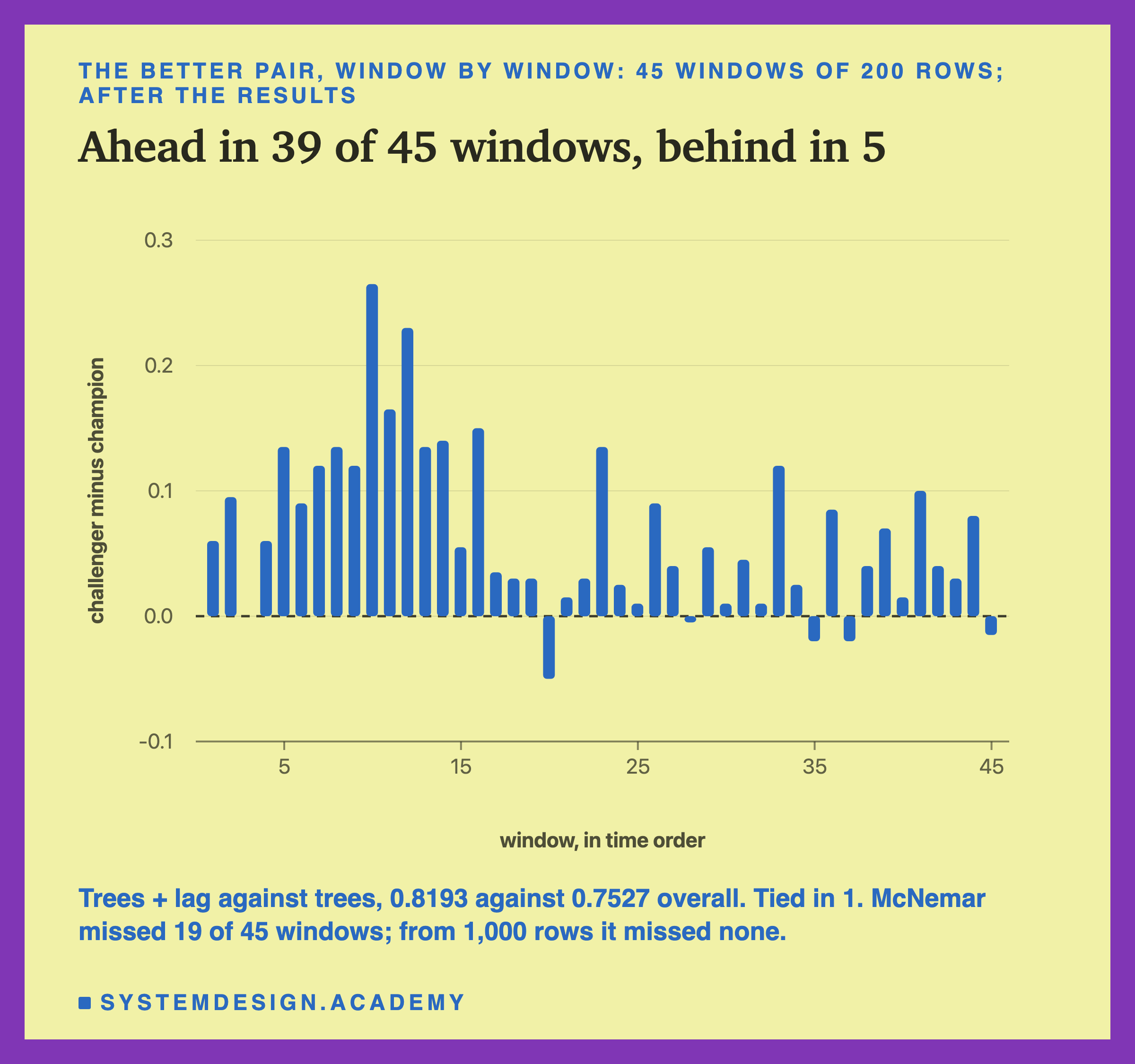
Window by window, with 200 rows the better model was ahead in 39 of the 45 windows, tied in 1 and behind in 5. The gap in one window ranged from -5.0 to +26.5 points. So even a model that is better by 6.7 points overall loses some short windows. The naive and margin rules promoted it in 0.867 of windows, and McNemar in only 0.578: it missed 19 of the 45. In 6 of those the challenger was not ahead at all (5 behind, 1 tied), so no rule could promote. In the other 13 its lead rested on too few disagreeing rows: a median of 18 across the missed windows, against 24 over all 45.

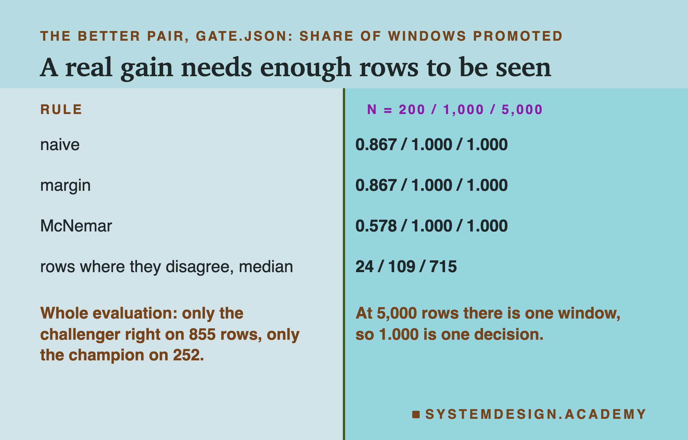
With 1,000 rows every rule caught it in all 9 windows; the smallest window gain was +3.6 points. With 5,000 rows, every rule caught it too, but that is a single window, so it is one decision, not a rate.

So a careful rule costs something. McNemar made far fewer false promotions than the other two, and in exchange it needed more rows to see a real gain. That is not a flaw to fix by lowering the bar. Every gate makes this trade, and the answer is more rows, not a looser rule. How many rows are enough depends on the size of the gain you care about: here McNemar caught a 6.7-point gain in 0.578 of 200-row windows and in all 9 windows of 1,000 rows; sizes in between were not tried. A 1-point gain would need many more, and I did not measure how many.

The follow-up had a second question. A real gate sees the most recent rows, one block after another, and neighbouring half-hours are alike: lesson 1 found the label repeats the previous one 85.3% of the time. McNemar's test assumes each disagreeing row is a separate coin toss. If neighbouring rows go the same way, a block of them could look more uneven than chance allows, and the test would be fooled more often than 5% of the time. People call that inflating the test.

So the follow-up also scored the same true-null pairs on N rows drawn at random from the whole evaluation, 200 draws per pair and size. If McNemar were near 5% on random rows but higher on contiguous windows, the neighbouring rows would be to blame.

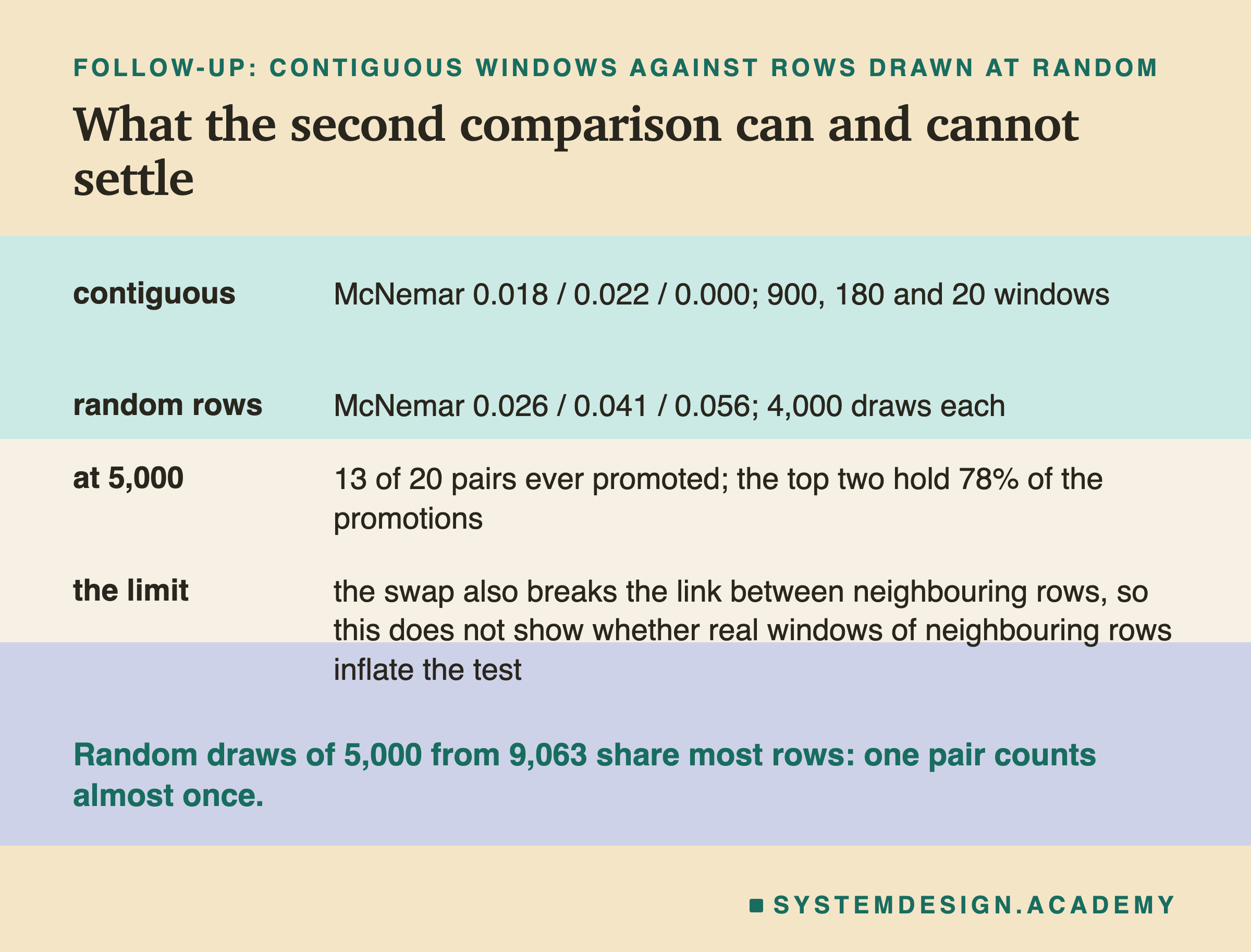
It came out the other way: contiguous windows promoted less often than random rows. But that does not show that contiguous windows are safe, and I only saw why after the run. The swap tosses a new coin on every row. So after the swap, which model got one row tells you nothing about which model got the next row. The swap removed the very link between neighbours that I wanted to test. So this comparison cannot tell whether real windows of neighbouring rows inflate the test. I leave that question open.

The random-row numbers have a second problem, which I found by reading the draws pair by pair. At 5,000 rows, one random draw takes more than half of the 9,063 evaluation rows. So the 200 draws of one pair share most of their rows, and they mostly give the same answer. McNemar promoted in 13 of the 20 pairs at least once, but two pairs held 78% of all its promotions. In those two pairs, the coins happened to leave the challenger ahead over the whole evaluation. So the 0.056 behaves more like "2 of 20 pairs" than like a rate from 4,000 separate tries.

One more way a gate is fooled has nothing to do with the rule. A team trains a challenger, checks it against the champion, and it fails. A day later, with more rows, they check again. And again. Each check is a new chance for luck to push the challenger over the line, and the gate only needs to pass once.

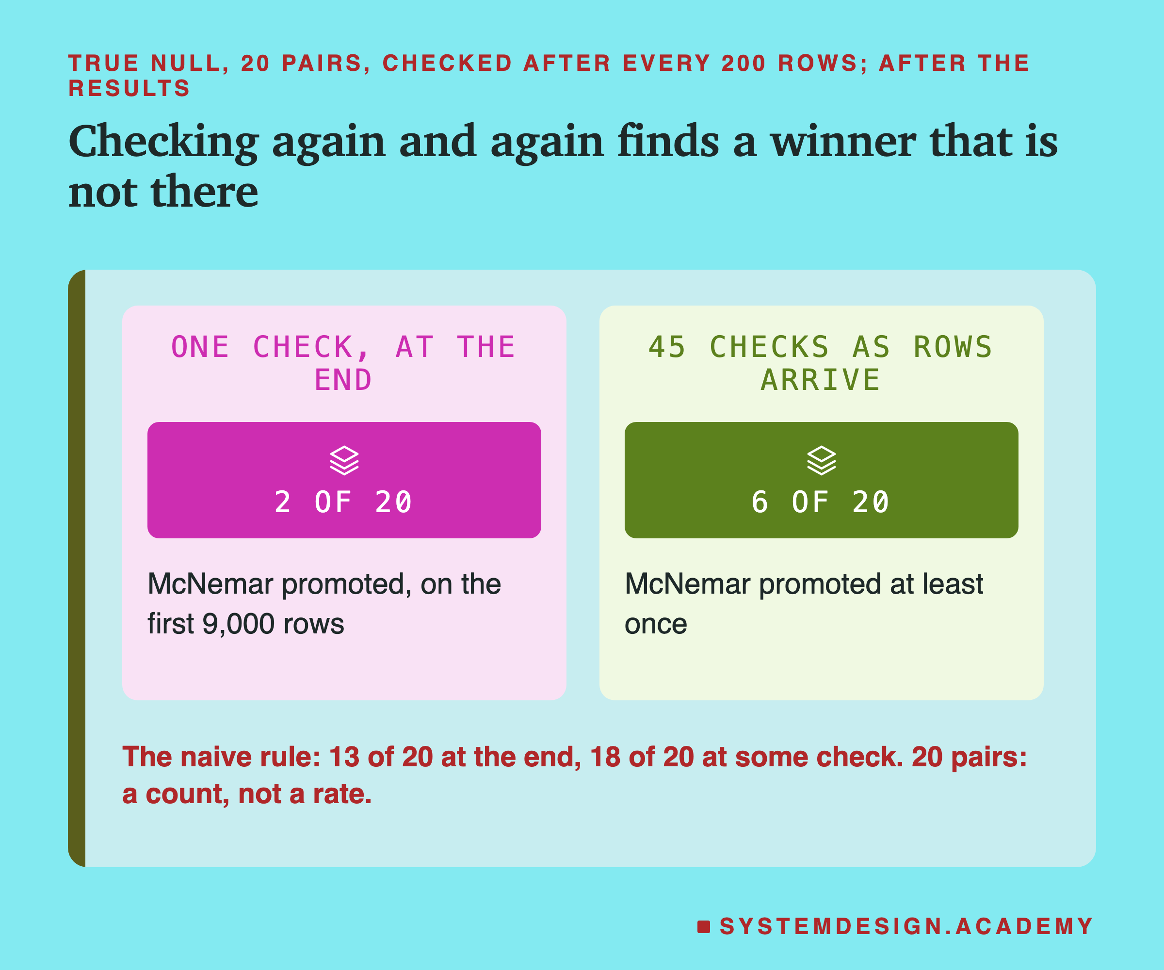
I measured this on the 20 true-null pairs. For each pair I checked the gate after every 200 new rows, each time on all the rows so far: 45 checks, up to 9,000 rows. With one check at the end, McNemar promoted 2 of the 20 equal challengers. Checking 45 times as the rows arrived, it promoted 6 of the 20 at some point. The naive rule went from 13 to 18 of 20. With 20 pairs these are counts, not rates, but the direction is the one the reasoning predicts: every extra look is another chance to be fooled.

The fix is to decide in advance when you will look, and to look once, or to use a method built for repeated looks, which demands a stricter bar at each look. A later lesson in this chapter measures this same effect on live traffic, where checking after every batch of requests is exactly what a team wants to do.

Here is what the lab points to, in the order a team meets it.

Score both models on the same rows. A paired comparison is only possible when both models answer the same rows. Keep a fixed evaluation set, or a fresh window, and score the champion again on it rather than reusing an old score from different rows.

Write the rule down before anyone sees a score. The rule, the threshold and the window size all belong in the pipeline's code or configuration, fixed in advance. Changing the rule after seeing that the challenger narrowly failed is a form of the winner's curse that lesson 3 measured: a choice made after seeing the scores flatters itself.

Use a paired test, not a raw comparison. McNemar's test for right-or-wrong answers counts only the rows where the two disagree, and it held near 5% on equal models here, where "higher wins" promoted about half of them. It needs nothing beyond counting and a few lines of arithmetic. Note what the swap test can and cannot show: under the swap, McNemar holding near 5% is what the maths requires, because the swap builds exactly the coin-flip assumption the test rests on. The lab's new evidence is about the other two rules. And even a test that holds at 5% is fooled about one time in twenty: a weekly retrain between equal models gives up to about 2.6 false promotions a year (52 × 0.05, arithmetic).

Choose the window size for the gain you care about. A small window cannot see a small gain, and a careful rule on a small window will say no to real improvements. Here McNemar caught a 6.7-point gain in 0.578 of 200-row windows and in all 9 windows of 1,000 rows; sizes in between were not tried. Decide what gain is worth promoting, then use enough rows to see it.

Check once, or correct for checking often. Every extra look at the same comparison is another chance for luck. Here, 45 looks turned 2 false promotions into 6.

Log the decision. Record the rule, the rows, the four counts and the p-value with every promotion. When someone asks later why a model went live, that record is the answer, and it makes a bad promotion something you can find and undo.

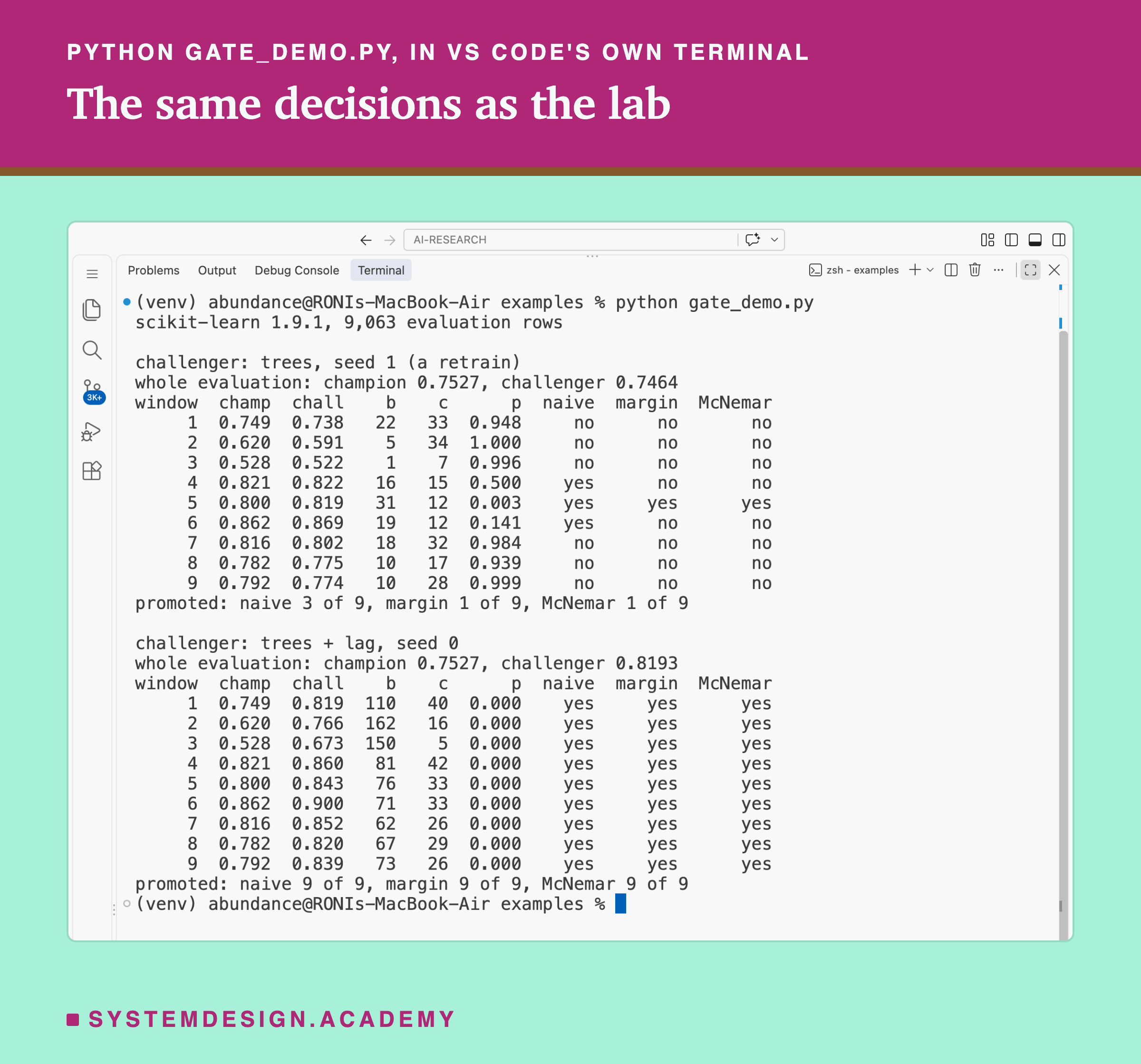
This script is the lab made small. It downloads the same data, trains the champion (the trees with seed 0) and two challengers (the trees with seed 1, like a scheduled retrain, and the trees plus lag), cuts the evaluation into windows of 1,000 rows, and prints each rule's decision in every window. It does not need a GPU.

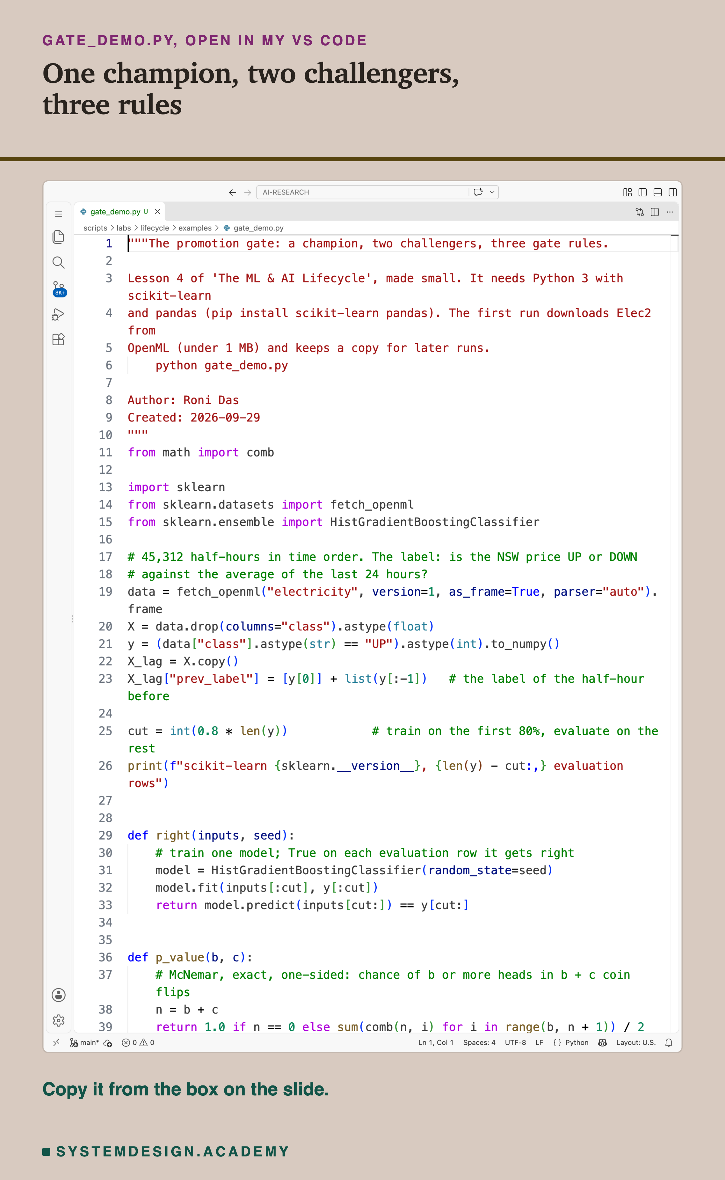
Before you run this lab. You need Python 3 and two libraries: pip install scikit-learn pandas. scikit-learn holds the model and the download; pandas holds the table. The first run downloads Elec2 from OpenML (under 1 MB compressed), so it needs an internet connection once; scikit-learn keeps a copy in a folder in your home directory (scikit_learn_data) for later runs. McNemar's test needs no extra library: it is a sum of counts from Python's own math.comb. I ran it with scikit-learn 1.9.1 on a Mac. scikit-learn runs the same way on Windows and Linux, but I have not checked the numbers there, and another version of scikit-learn may give different decimals, which is why the first line printed is the version.

"""The promotion gate: a champion, two challengers, three gate rules.

Lesson 4 of 'The ML & AI Lifecycle', made small. It needs Python 3 with scikit-learn
and pandas (pip install scikit-learn pandas). The first run downloads Elec2 from
OpenML (under 1 MB) and keeps a copy for later runs.
    python gate_demo.py

Author: Roni Das
Created: 2026-09-29
"""
from math import comb

import sklearn
from sklearn.datasets import fetch_openml
from sklearn.ensemble import HistGradientBoostingClassifier

# 45,312 half-hours in time order. The label: is the NSW price UP or DOWN
# against the average of the last 24 hours?
data = fetch_openml("electricity", version=1, as_frame=True, parser="auto").frame
X = data.drop(columns="class").astype(float)
y = (data["class"].astype(str) == "UP").astype(int).to_numpy()
X_lag = X.copy()
X_lag["prev_label"] = [y[0]] + list(y[:-1])   # the label of the half-hour before

cut = int(0.8 * len(y))            # train on the first 80%, evaluate on the rest
print(f"scikit-learn {sklearn.__version__}, {len(y) - cut:,} evaluation rows")


def right(inputs, seed):
    # train one model; True on each evaluation row it gets right
    model = HistGradientBoostingClassifier(random_state=seed)
    model.fit(inputs[:cut], y[:cut])
    return model.predict(inputs[cut:]) == y[cut:]


def p_value(b, c):
    # McNemar, exact, one-sided: chance of b or more heads in b + c coin flips
    n = b + c
    return 1.0 if n == 0 else sum(comb(n, i) for i in range(b, n + 1)) / 2 ** n


champion = right(X, 0)
challengers = {"trees, seed 1 (a retrain)": right(X, 1),
               "trees + lag, seed 0": right(X_lag, 0)}

for name, challenger in challengers.items():
    print(f"\nchallenger: {name}")
    print(f"whole evaluation: champion {champion.mean():.4f}, "
          f"challenger {challenger.mean():.4f}")
    print("window  champ  chall    b    c      p  naive  margin  McNemar")
    total = {"naive": 0, "margin": 0, "McNemar": 0}
    for w, start in enumerate(range(0, len(champion) - 999, 1000), 1):
        cm, ch = champion[start:start + 1000], challenger[start:start + 1000]
        b = int((ch & ~cm).sum())          # rows only the challenger got right
        c = int((cm & ~ch).sum())          # rows only the champion got right
        gap = ch.mean() - cm.mean()
        p = p_value(b, c)
        said = {"naive": gap > 0, "margin": gap >= 0.01,
                "McNemar": gap > 0 and p < 0.05}
        for rule in said:
            total[rule] += said[rule]
        yes = ["yes" if said[r] else "no" for r in said]
        print(f"{w:>6}  {cm.mean():.3f}  {ch.mean():.3f}  {b:>3}  {c:>3}  {p:.3f}"
              f"  {yes[0]:>5}  {yes[1]:>6}  {yes[2]:>7}")
    print(f"promoted: naive {total['naive']} of {w}, margin {total['margin']} of {w},"
          f" McNemar {total['McNemar']} of {w}")

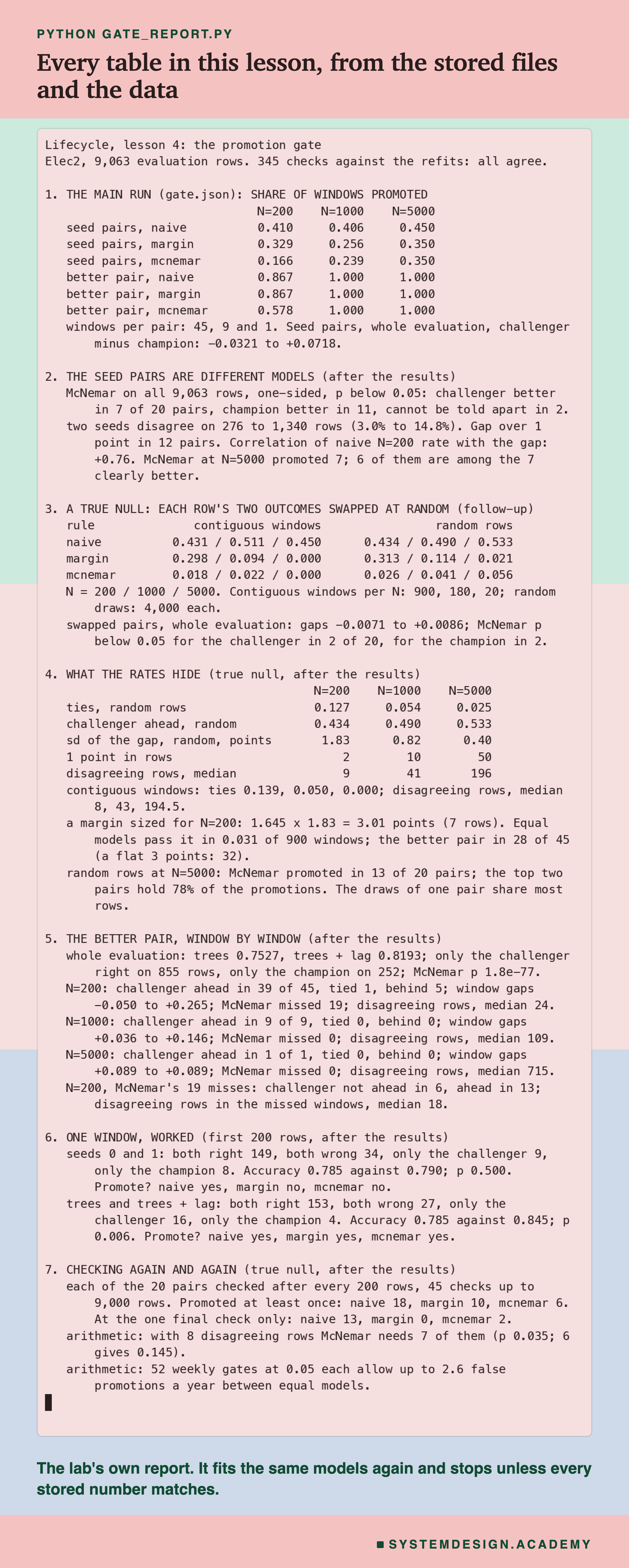
The report lives in scripts/labs/lifecycle/gate_report.py. It reads the lab's stored files, results/gate.json and results/gate_followup.json, lessons 1 and 2's stored files, and the Elec2 data from scikit-learn's local copy. The lab stored promotion rates, not each model's right and wrong rows, so the report trains the lab's 41 models again with the same data, split and settings. It stops unless every stored number comes back exactly: each model's accuracy on the whole evaluation, every pair's rate for every rule and window size, and the follow-up's true-null rates, which it rebuilds with the follow-up's own coin seed and draw seed. It makes 345 checks in all, and they all agree. It changes nothing in the lab's files.

Its json mode writes every number to results/gt-report.json, which the figures read. The demo mode checks the student script's stored run, and the box mode writes the playground below and checks that it gives the lab's rates.

This box has no model in it. It holds the real right-or-wrong outcome of seven models on all 9,063 evaluation rows: the trees with seeds 0 to 5 and the trees plus lag. Each row's seven outcomes are packed into two hexadecimal digits (counting in sixteens, with the digits 0 to 9 and a to f), and the right function unpacks one model's column. The report checked every rate it prints against gate.json. It runs in your browser.

As it is, the box prints the promotion rates of three pairs at each window size, exactly the lab's: seeds 0 and 1, seeds 4 and 5 (a pair where the challenger was 7.2 points better on the whole evaluation) and the trees plus lag.

Now build a true null yourself: a, b = swapped(right(0), right(1)) and then rates(a, b). The box tosses its coins with Python's own random numbers, not the lab's, so it lands near the follow-up's rates, not on them; try a few values of seed. Then try peek(a, b), which checks McNemar after every 200 rows and returns the first row count at which it promoted, or None, and compare peek(a, b, rule='naive').

Loading. fetch_openml("electricity", version=1) downloads Elec2 once and reads the local copy after that. The label column holds the words UP and DOWN, turned into 1 and 0. X_lag is a copy of the inputs with one extra column, the previous half-hour's label, as in lesson 1.

The cut. cut = int(0.8 * len(y)) is 36,249. Every model learns from the rows before it and is evaluated on the 9,063 rows after it.

right. Trains one boosted-trees model with the given seed and returns, for every evaluation row, True if the model got it right. This one list per model is all a gate needs: the champion's list and the challenger's list, row by row.

p_value. McNemar's test, exact and one-sided. b is the number of rows only the challenger got right and c the number only the champion got right. It adds up the ways b + c fair coin tosses could give b or more heads, using math.comb, and divides by all the ways. No statistics library is needed.

The windows. range(0, len(champion) - 999, 1000) gives the start of each 1,000-row window, nine of them. For each window, marks the rows where only the challenger was right, and the rows where only the champion was.

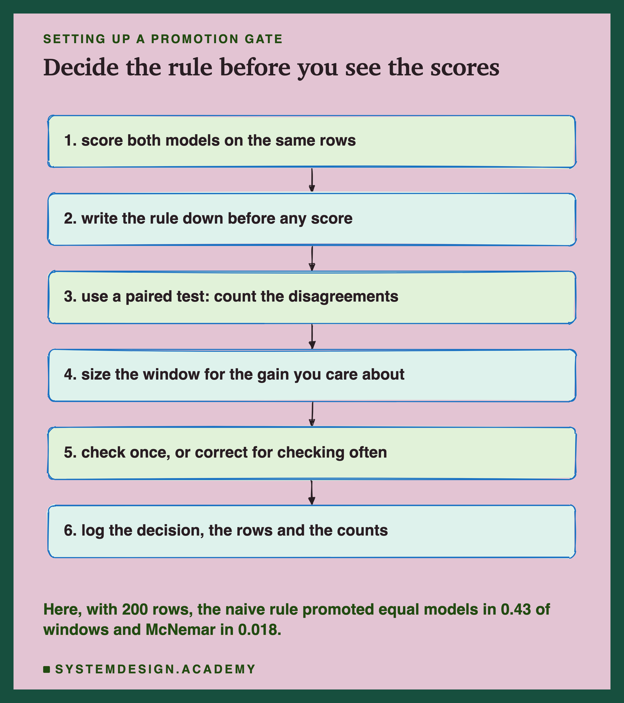
Score both models on the same rows. Keep the champion's predictions for the evaluation rows, or score it again, so that every row has two outcomes side by side.

Write the rule down before any score. Put the test, the 0.05 line and the window size in the pipeline's configuration, and review changes to it like changes to code.

Use a paired test. For right-or-wrong answers, McNemar's test. Count the four boxes, keep the two that disagree, and compute the p-value.

Size the window. Decide the smallest gain worth a promotion, then check, with a pair of models you know differ by about that much, that your window catches it most of the time. If it does not, collect more rows before deciding.

Check once, or correct. Decide when the gate runs. If it must run again and again as rows arrive, use a method built for repeated looks rather than the same 0.05 line each time.

Log the decision. The rule, the rows, the four counts, the p-value and the outcome, next to the model's run receipt from lesson 2, the record of code, seed, data, settings and versions that lets a run be repeated.

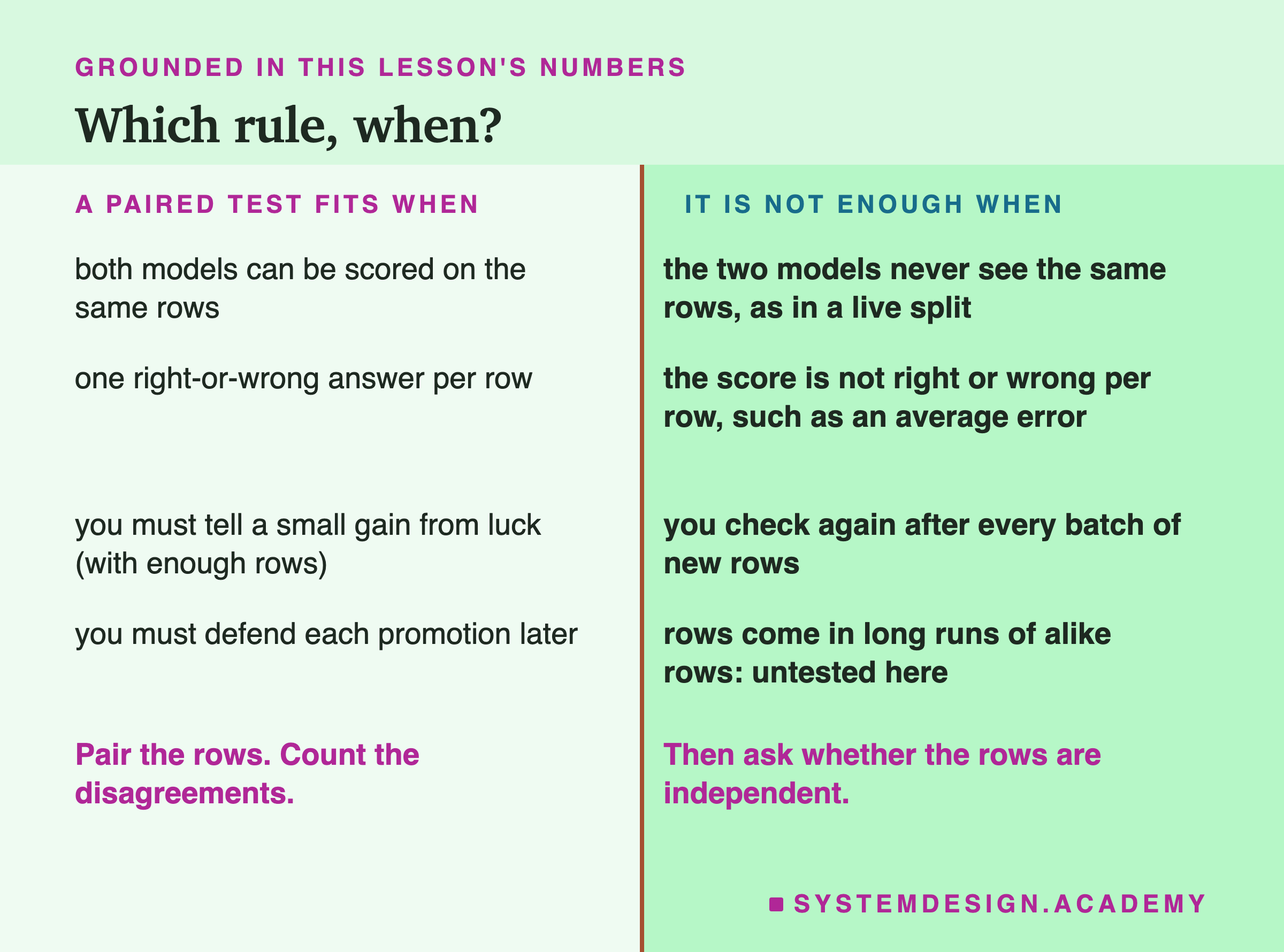
Use McNemar's test when both models answer the same rows, right or wrong. That is the usual offline gate: a fixed evaluation set, or the latest window of labelled rows, scored by both models. Here it held at or below about 5% on equal models. Under the swap that is what the maths requires, since the swap builds the test's own assumption; the lab's new evidence is how badly the other two rules did.

Use it when the gain you want is small. The naive rule cannot tell a small gain from luck, and a fixed margin mostly measures the window size. A paired test adapts to the rows that matter.

Use it when you will need to explain a promotion. The four counts and a p-value are a record anyone can check.

Do not use it when the two models never see the same rows. In a live test where each user is sent to one model or the other, there are no paired rows; that needs an unpaired comparison, which compares two separate groups of rows instead of the same rows twice, and a later lesson in this chapter deals with live traffic.

Do not use it as it stands when the score is not right or wrong. For an average error or a ranking score, a paired test for numbers is needed instead; McNemar's test only counts disagreements.

Do not rely on it alone when the rows come in runs. This lab did not settle whether neighbouring rows fool the test. If your rows are strongly alike in time, spread the window over a longer period or check the test on a pair you know to be equal, as the follow-up did.

Do not use the naive rule for anything that matters. Here it promoted an equal model in about half of all windows, at every size.

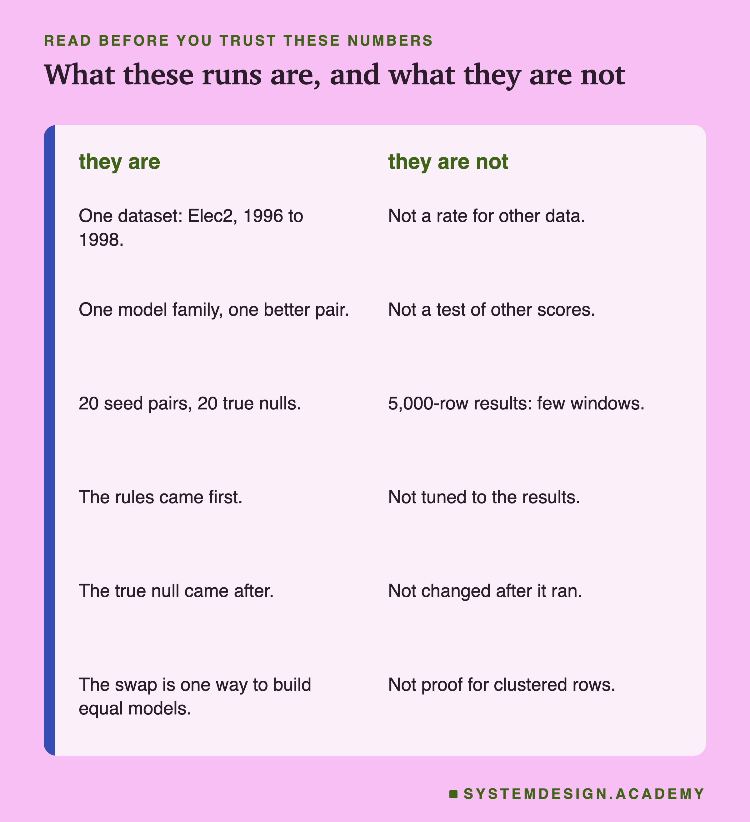
One dataset, one model family. Everything here is boosted trees on Elec2. The rates depend on how often two models disagree, which was 3.0% to 14.8% of rows for these pairs. With models that disagree more or less, the numbers would move. The better pair is one gain of one size, 6.7 points.

The main run's pairs were not null. The design called the seed pairs null; the results showed they were not. I have kept their numbers but not called them false-promotion rates. The true null is a follow-up, designed after the main results and written down before it ran.

The swap is one way to build equal models. It makes the two models equal row by row, and in doing so it also breaks any link between neighbouring rows. Real equal models could make errors in runs, and this lab cannot say what that does to the test.

Few windows at 5,000 rows. Each pair has one 5,000-row window, so those numbers are 20 decisions, and the random-row draws of one pair share most of their rows. Read the 5,000-row numbers as counts, not rates.

After the results. McNemar on each pair's whole evaluation, the ties, the standard deviation of the gap, the rows each window disagrees on, the better pair window by window, the worked windows and the repeated checks were all measured after I saw the results. The repeated checks cover 20 pairs: a count, not a rate.

No test of the rates themselves. The design described rates and declared no significance test on them. The p-values in this lesson belong to the gate's own decisions, not to the comparison of rules.

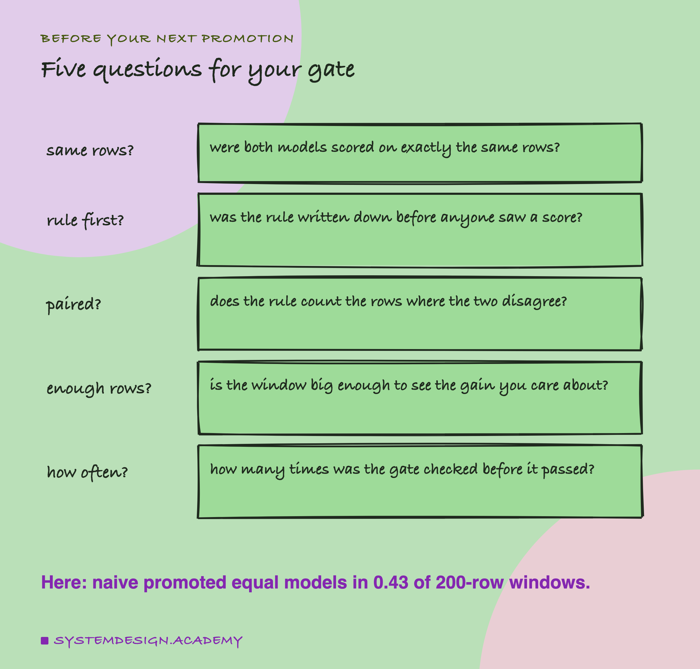
Find the rule your pipeline uses to promote a model, and ask the five questions on the card. If the rule is "the new score is higher", replace it. If it has a margin, find out how many rows it is applied to and whether the margin means anything at that size.

Then run a small version of this lab on your own data. Take your current model and a retrain with a different seed, score both on your evaluation rows, and count the rows where they disagree. That one number tells you how many rows your gate is really deciding on. Then build a true null by swapping outcomes at random, as the follow-up did, and see how often your rule promotes it.

The next lesson planned for this chapter moves the gate into production. A canary release sends a small share of live traffic to the new model; a shadow release runs the new model on live traffic without using its answers. That lesson measures how much traffic it takes to see that a new model is worse.