The Shelf Where Similar Things Sit
Let me start with a small picture.
Imagine a library where the librarian has read every book. She does not shelve the books by their number. She puts books that feel alike next to each other: cookery here, birds there, old maps in the corner. When you ask for something, she points at a shelf, not at one book.
Now suppose she wants to guess which readers will come back next month. She could look at how often each reader came, and how recently. Or she could look at which shelves each reader took books from. The shelves sound richer. They say something about taste. But will they help her guess who comes back? Taste and loyalty are not the same thing.
This lesson asks the same question about a real shop. Every product has a name. A computer can place names that mean similar things close together, like the librarian's shelves. I measure whether that helps a model guess which customers will buy again.
Where This Lesson Starts
This lesson uses the same shop, the same customers and the same question as the rest of the chapter. If any of that is new, please read what a feature is first. It sets up the data and the task. It also built six simple facts about each customer, which I reuse here as the starting point. They are how recently they bought, how often, and how much they spent. The other three are how much they sent back, how long they have been a customer, and how many different products they bought.
Lesson 7, on categorical features at scale, gave the model the product CODES a customer bought. A code like 85123A is only a label. It says nothing about the product. The best result there came from filing codes into numbered drawers, and the gain was tiny.
This lesson gives the model the product NAMES instead, turned into numbers that carry meaning. If meaning matters, this is where it should show.
What an is, and how two of them are compared, is taught in the tokens and embeddings chapter: what an embedding is and cosine, dot and distance. I do not teach it again here. I only use it.
The Words You Need First
Please read this slide slowly if any word is new. Every slide after it uses these words.
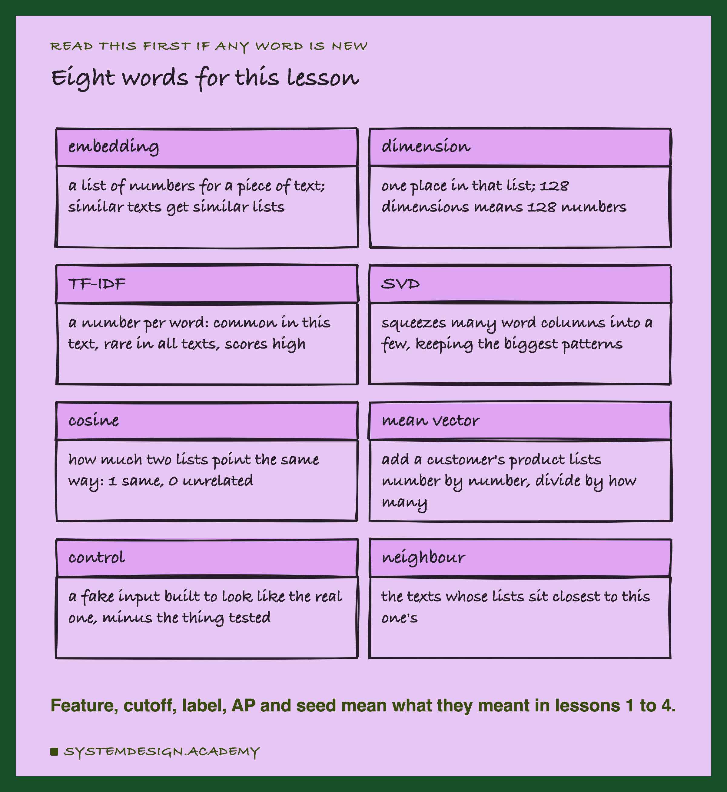
. A list of numbers that stands for a piece of text. A good embedding model gives texts with similar meaning similar lists. Each list is also called a vector.
Dimension. One position in the list. A vector with 128 dimensions is a list of 128 numbers.
TF-IDF. An older way to turn text into numbers, with no neural model. TF means term frequency: how often a word appears in this text. IDF means inverse document frequency: a word that appears in few texts gets a bigger weight than a word that appears in many. Each word gets its own column.
SVD. Short for singular value decomposition. Here it squeezes thousands of word columns into a few, such as 64, keeping the patterns that explain the most. scikit-learn's page says that, used on TF-IDF like this, it is known as latent semantic analysis, or LSA.
Cosine. A measure of how much two vectors point the same way. 1 means the same direction, 0 means no relation.
Mean vector. For one customer, add up the vectors of every product they bought, number by number, and divide by how many products there were.
Control. A fake input, built to look like the real one in every way except the thing being tested. If the real one cannot beat the control, the thing being tested did not help.
Feature, cutoff, label, average precision (AP), ROC-AUC and seed mean what they meant in lessons 1 to 4.
From Many Product Names to One List
A row in this chapter is one customer at one cutoff date. But a customer buys many products, and each product name becomes a vector. So I need one list per row.
I used the simplest rule: the mean of the vectors of every distinct product the customer bought before the cutoff. Each product counts once, however often it was bought. Returns do not count. A customer whose only lines before the cutoff are returns gets empty values, which this model handles by itself. That happened on 960 train rows and 311 test rows.
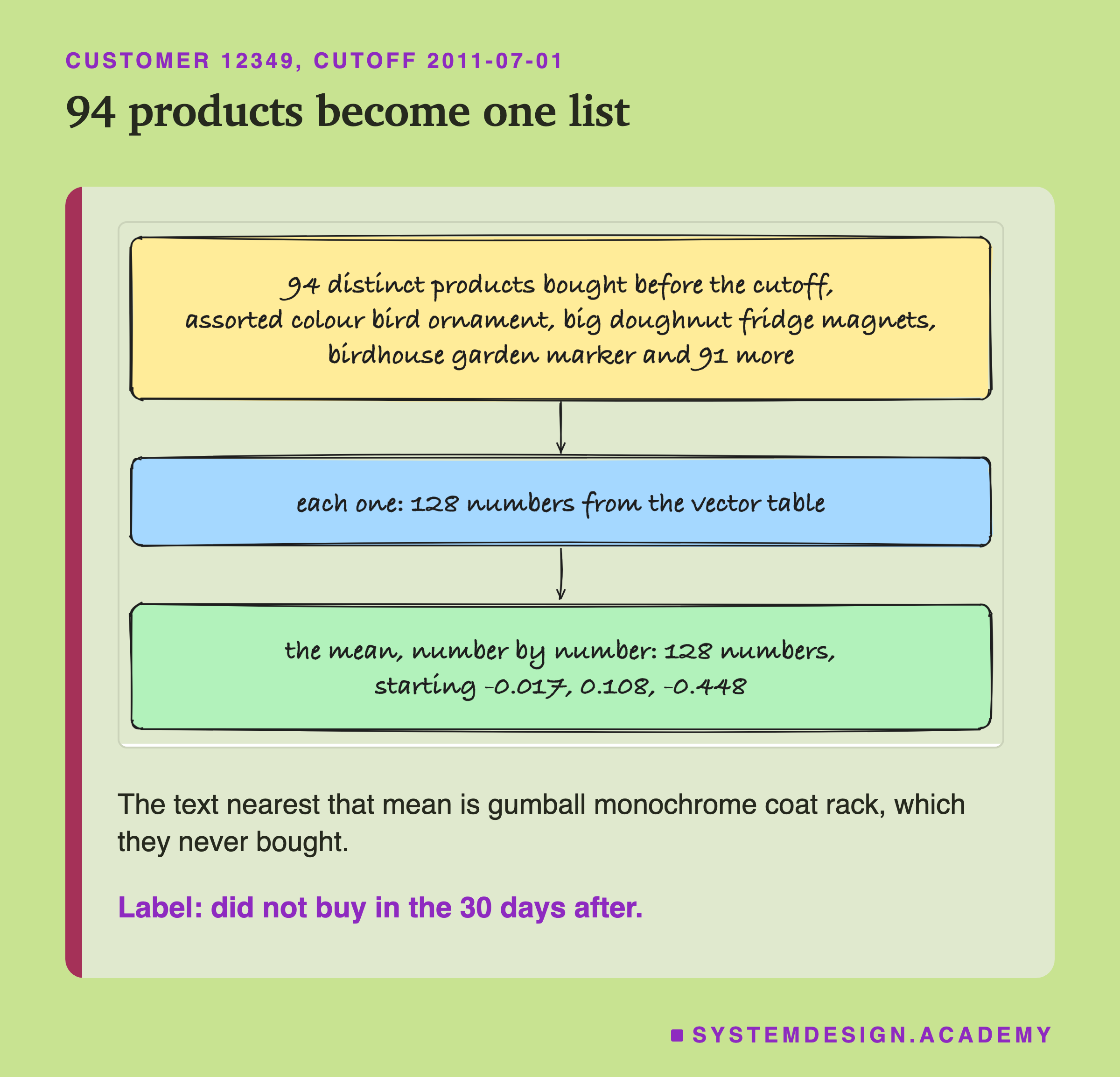
Here is one real customer, number 12349 at the cutoff 1 July 2011, the same customer lessons 1 and 7 used. They had bought 94 different products. The lab looked up the 128 numbers of each one and took their mean.
Then I asked which product name sits nearest to that mean. The answer was a gumball monochrome coat rack, a product this customer never bought. The second nearest, a bubblegum ring, they never bought either. A mean of 94 different things looks like none of them. Keep that in mind; it comes back later.
I also tried a second rule, declared before the run: a mean weighted by spend, so a product the customer spent more on counts for more. On 26 train rows and 10 test rows every weight was zero, so those rows fell back to the plain mean.
Two Ways to Turn a Name Into Numbers
The shop's data holds 5,257 different product descriptions, once spaces at the ends are trimmed. I turned every one of them into numbers twice.
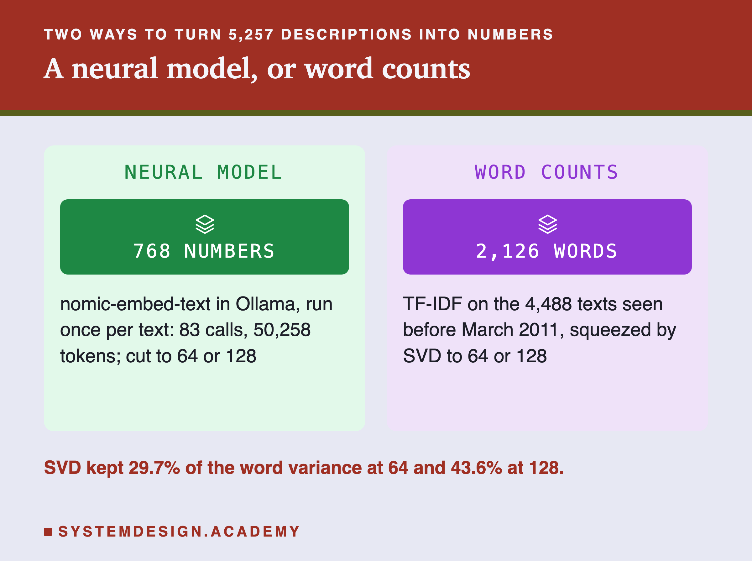
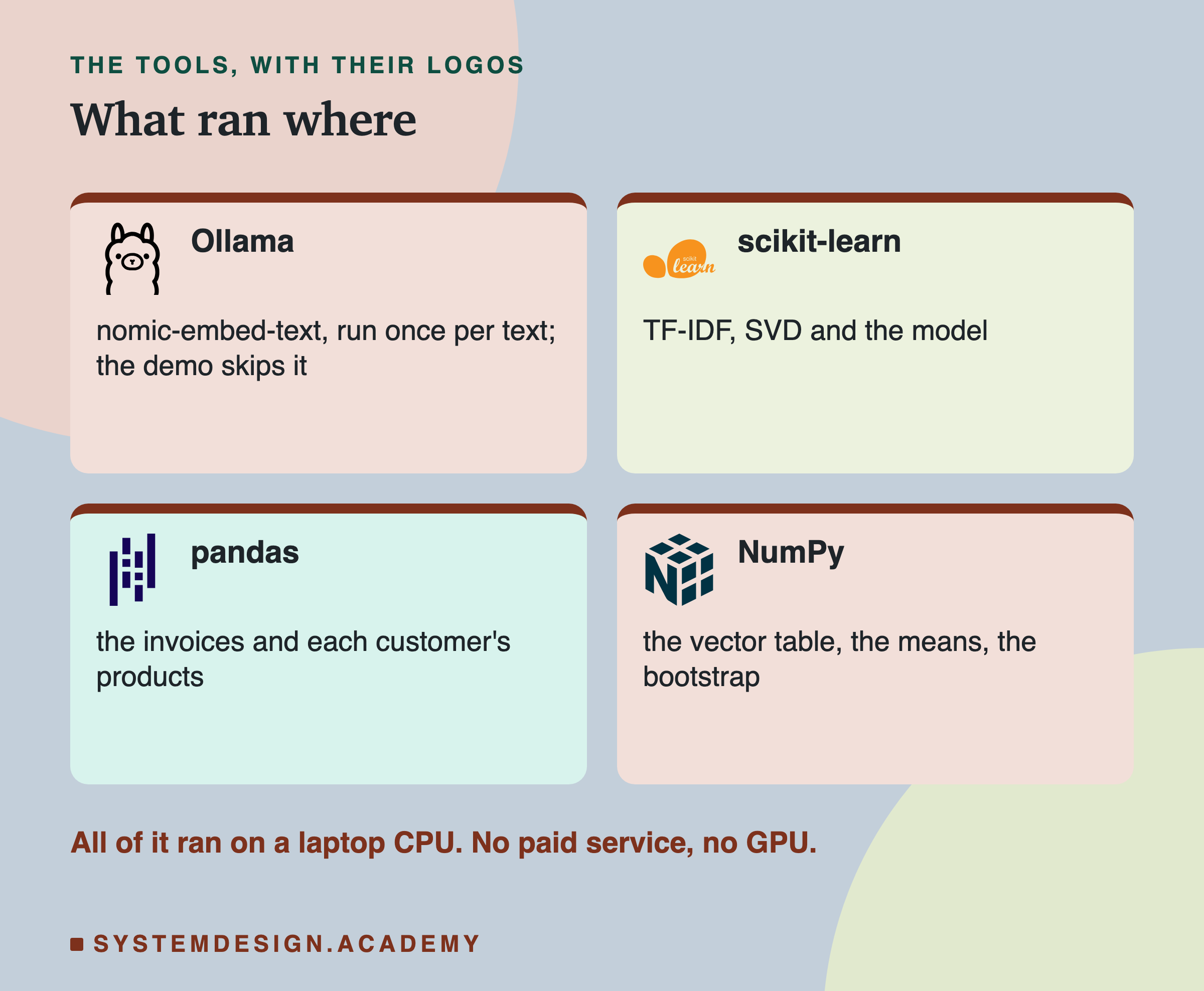
The neural model. I used nomic-embed-text, version 1.5, a small open model of about 0.1 billion parameters under the Apache 2.0 licence, running in Ollama on this laptop. It gives 768 numbers per text. Its model card asks for a short prefix before each text that says what the vectors are for. One prefix, "classification: ", is described as being for "texts into vectors that will be used as features for a classification model". That is exactly this lesson, so I used it. The whole job was 83 calls to Ollama, and Ollama reported 50,258 tokens read.
The word counts. TF-IDF with scikit-learn's default settings, then SVD down to 64 or 128 numbers. I fitted both only on the 4,488 descriptions that appear before 1 March 2011, the end of the training months. They found 2,126 different words. A later description whose words were all new gets a vector of zeros; that happened to 4 texts.
The SVD at 64 numbers kept 29.7 percent of the spread in the word table, and at 128 it kept 43.6 percent. The rest was thrown away.
Both ways were cut to the same two sizes, 64 and 128, so that each pair is a fair race at the same width.
Cutting 768 Numbers Down to 128
A model with 768 numbers per product would give each customer row 768 extra columns. That is a lot for a question this small. So I cut the neural vectors down to 64 and 128 numbers.
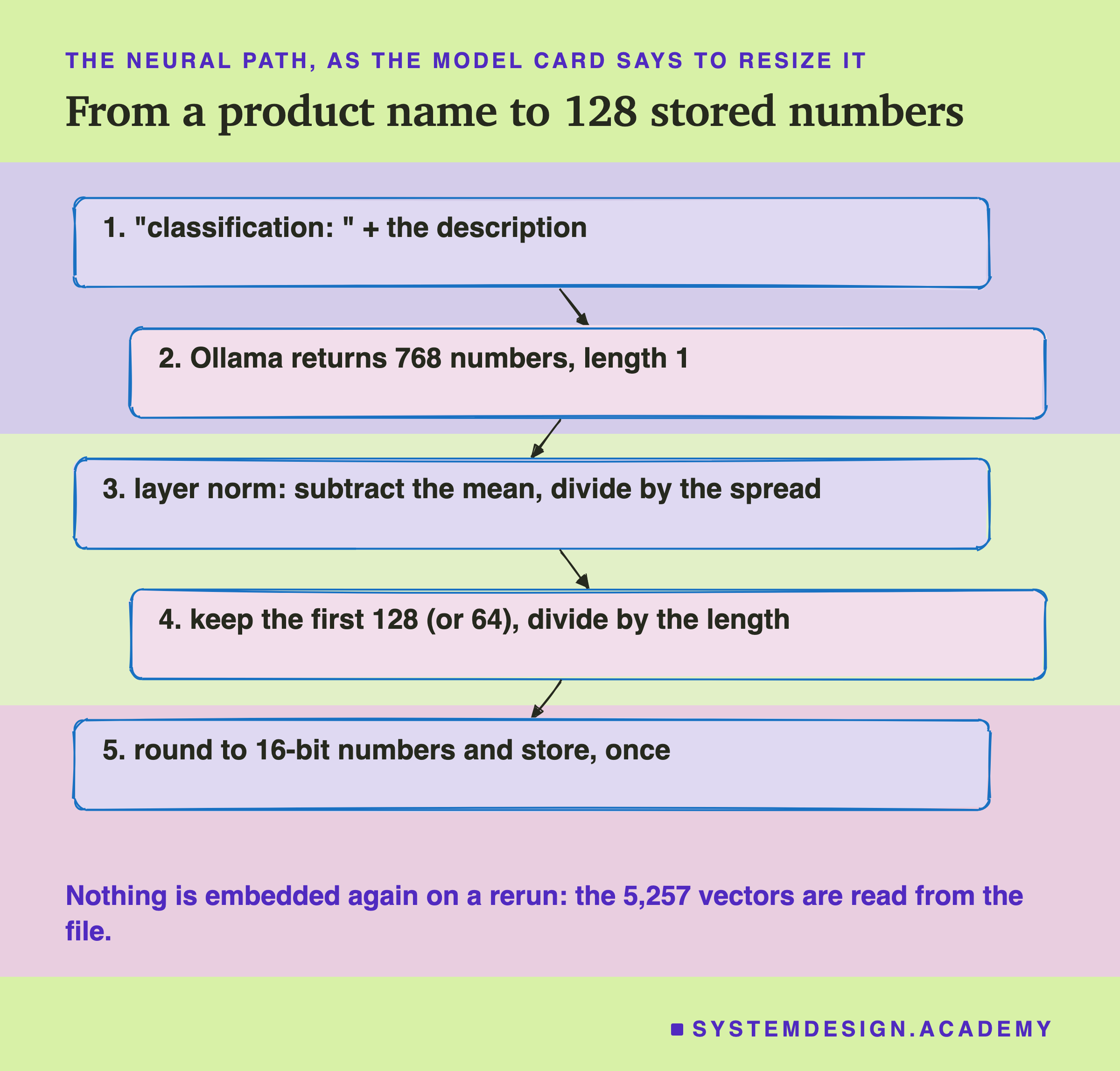
You cannot cut most by simply dropping numbers. This model was trained so that you can: its first numbers carry the most meaning. The chapter on embeddings has a lesson on shorter embeddings that measures this idea. The card gives three steps. First a "layer norm", which subtracts the vector's own mean and divides by its spread. Then keep the first numbers. Then divide by the length, so the result has length 1. The card also reports that the model scores lower on its own tests as the vector gets shorter.
Two practical points. The lab embeds each distinct text exactly once and keeps the result in a file. Run it again and it reads the file; it never calls Ollama twice for the same text. And the stored numbers are rounded to 16-bit floats, half the size of the usual 32-bit ones. Every feature in this lesson is built from those rounded numbers, so the report can rebuild everything from the stored file alone.
The Shop, the Task and the Split
The data is UCI Online Retail II, a public dataset under a CC BY 4.0 licence. It holds every sale of a UK online shop from 1 December 2009 to 9 December 2011. The shop mainly sells gift items, and many of its customers are wholesalers, people who buy to sell again. The chapter's fixed cleaning drops lines with no customer id and keeps returns as flagged rows.
The task is the chapter's fixed one. On the first of each month, for every customer seen before that day, will they buy in the next 30 days? Each pair of a customer and a cutoff is one row, and the label is 1 if they bought.
The rows are split by time. Train months, March 2010 to March 2011, give 44,521 rows; the models learn from these. Valid months, April to June 2011, give 14,673 rows; the one choice in this lesson is made here. Test months, July to November 2011, give 26,851 rows; they only score, and they choose nothing.
Average precision (AP) asks: when the model's list of likely buyers is read from the top, how many of the names near the top really bought? A random list scores about the share of buyers, which averaged 0.196 over the five test months. Every AP in this lesson is worked out per test month and then averaged over the five.
How the Lab Was Built
I wrote the lab's design into the docstring of scripts/labs/features/embeddings_features.py before it first ran. Before that I had looked at the data's columns, counted the distinct descriptions, and sent two descriptions to Ollama once to see the shape of what came back. No model had been trained on this task with any text.
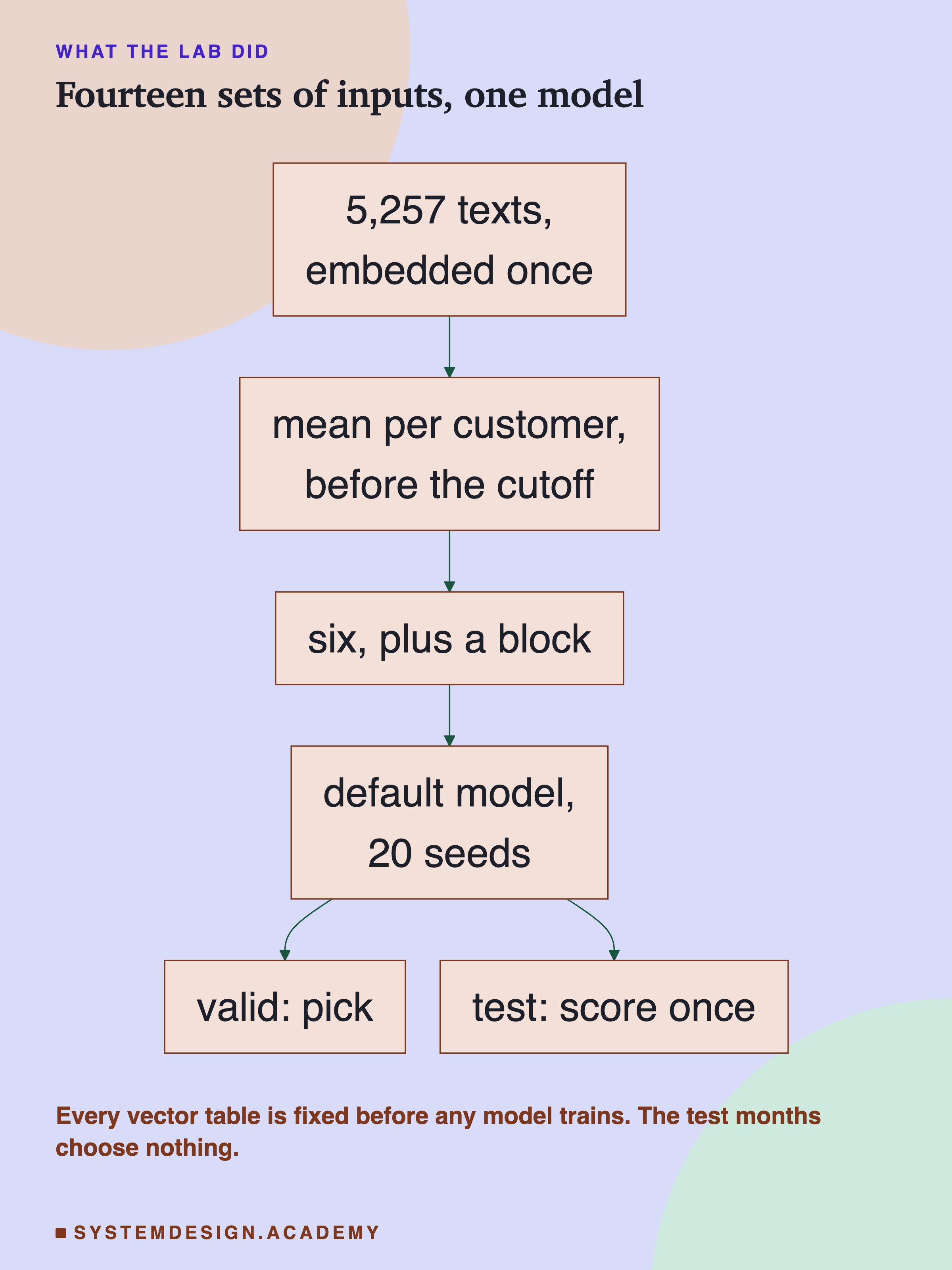
The model is the chapter's usual one: scikit-learn's HistGradientBoostingClassifier with its default settings. It builds many small decision trees, each one fixing the mistakes of the trees before it. Every contestant is lesson 1's six features plus one block of extra columns. Only the block changes.
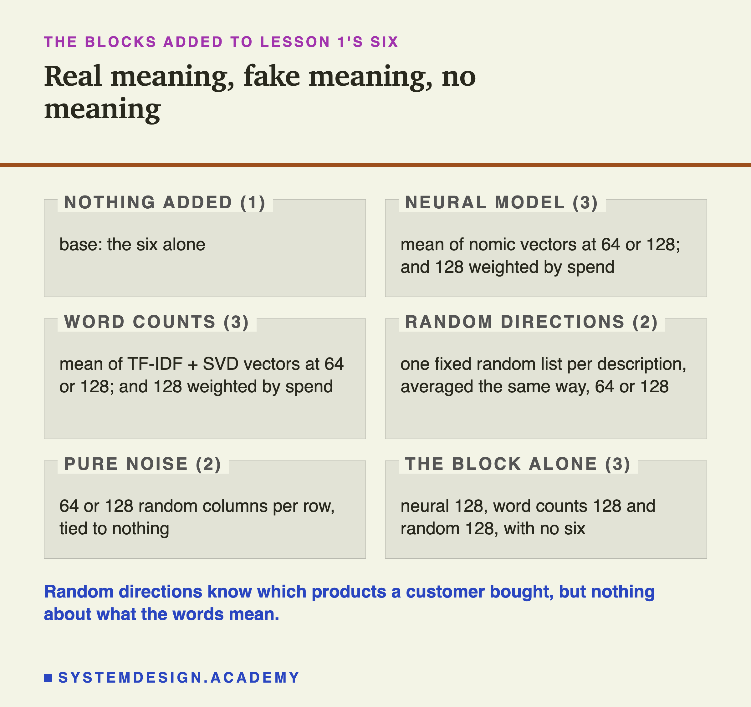
The two kinds of fake block matter most. Random directions give every description a fixed list of random numbers, then take the customer's mean the same way. This control knows exactly which products each customer bought, as the real do. It knows nothing about the names. Pure noise is just random columns, the same for nobody. It tests whether a model gains from more columns alone.
The design wrote down six guesses so they could be wrong in public. Here they are, scored.
-
No block beats the six by an interval clear of zero. Right for every real embedding. With the first random table, random directions at 64 did clear zero; over ten random tables, drawn after a review, they did not.
What the Vectors Put Together
Before any model, it is worth checking that the vectors do what they promise. For the three products bought on the most lines before March 2011, the lab listed the five nearest other descriptions in each vector table.
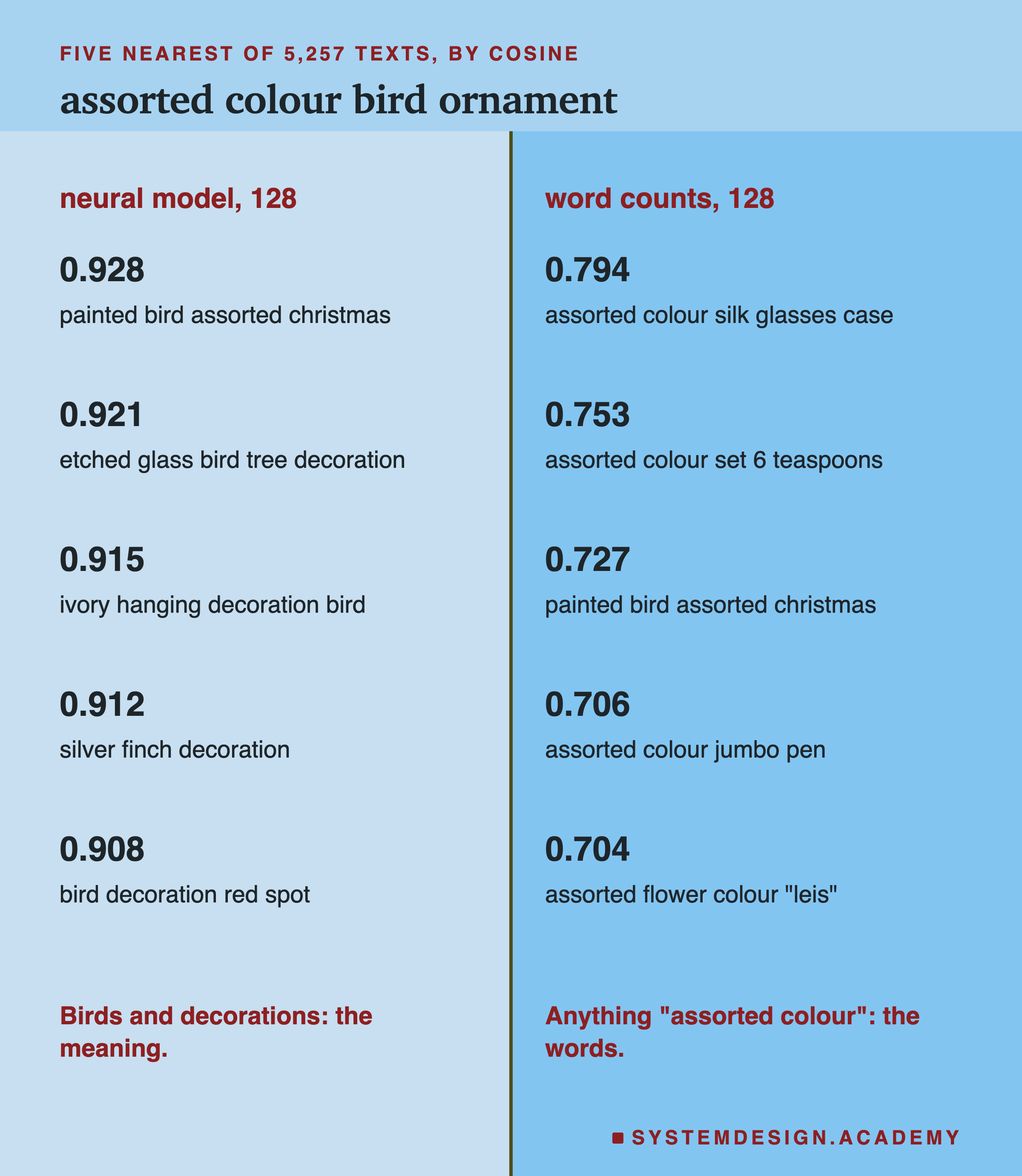
This one shows the difference best. The neural model found birds and decorations: a silver finch decoration, an etched glass bird. The word counts found anything that shares the words "assorted colour": a glasses case, teaspoons, a pen. Word counts match words, not meaning.
For the regency cakestand, both did well: the neural model's nearest was a sweetheart cakestand, 3 tier, at 0.934. For the white hanging heart t-light holder, both found other hanging heart holders. The random table found nothing in common at all; its nearest to the bird ornament began with a floral print tape.
Across all 5,257 texts, the 10 nearest neighbours in the neural table and in the word table shared 3.41 texts on average. The neural table and the random table shared 0.02. So the two real tables agree in part, and the random one agrees with nothing. It is a fair control.
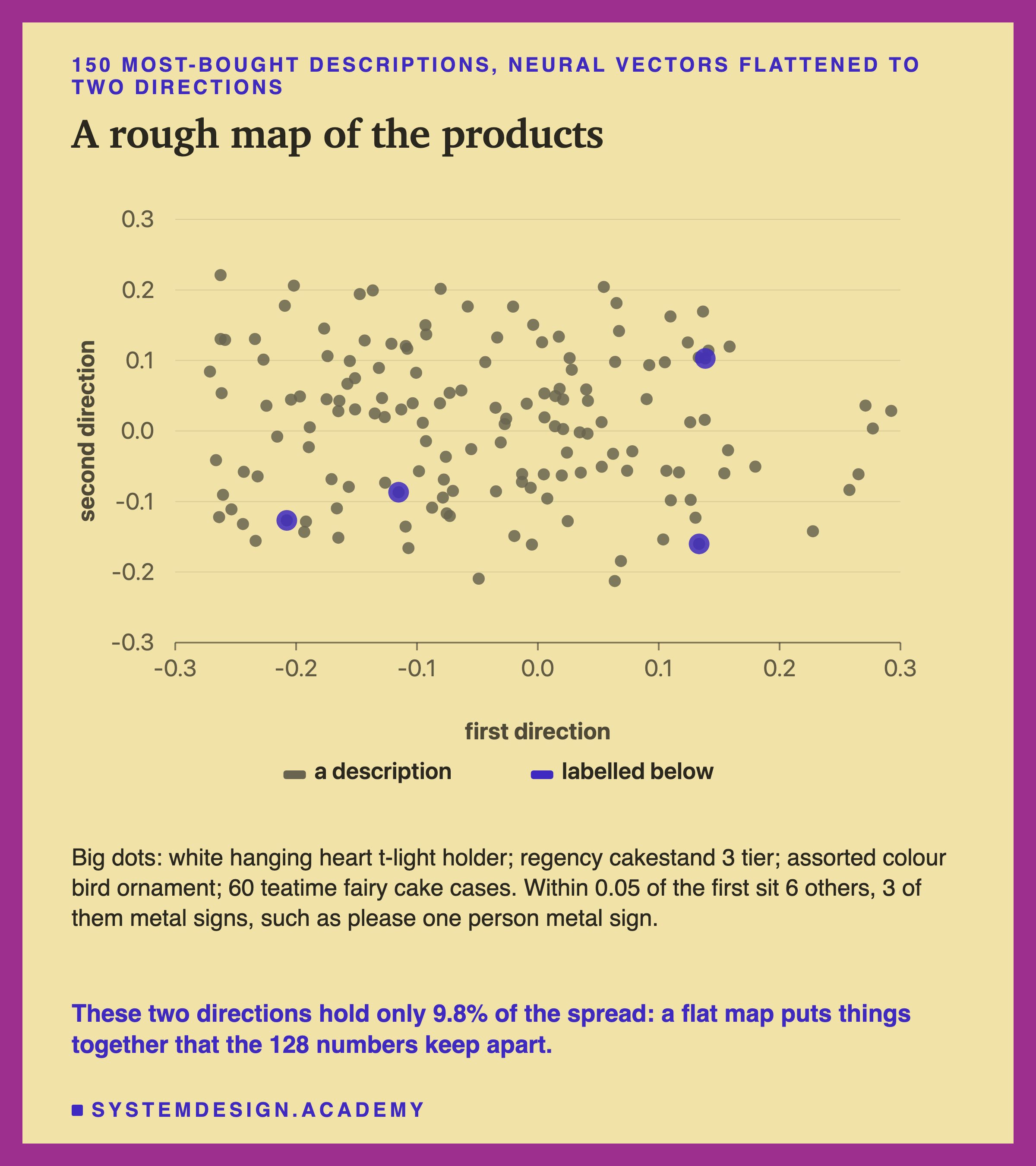
A map is tempting, so I drew one, after the results, as a picture and not a finding. It is honest only about its own weakness. The first two directions hold just 9.8 percent of the spread. On this flat map, three metal signs sit right next to the white hanging heart. None of them is among its five nearest in the full 128 numbers.
The Lab's Report, Running
This is a real recording of the report script, emb_report.py, on the laptop where the lab ran. It trains nothing new except four checks. It reads the stored results and the stored vectors, and checks every number this lesson uses.
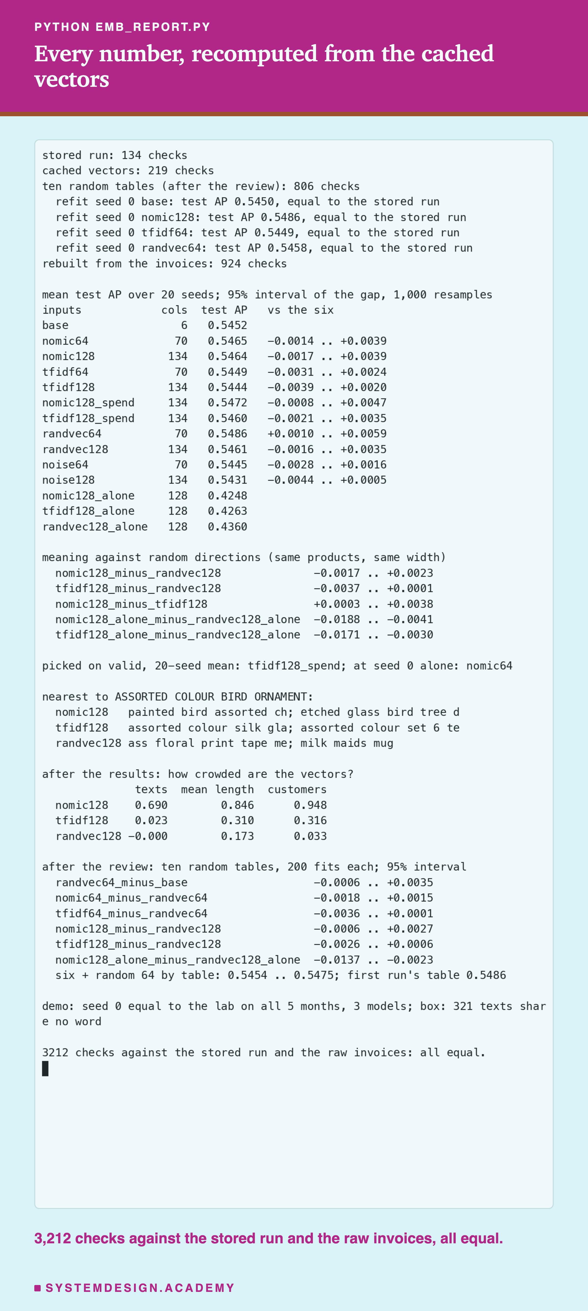
The report rebuilds every customer's mean vector from the raw invoices with its own, simpler code: a plain group-by mean per cutoff, not the lab's sparse table product. It compares those features with sums the lab stored, then retrains four models at seed 0 and checks their test scores to twelve decimal places.
It refits TF-IDF and SVD and checks that they give exactly the stored 16-bit vectors. If the raw 768-number file is present, it also redoes the model card's resize and checks those vectors. It recomputes the nearest neighbours, the overlaps, every mean of 20 seeds, every table mean of the ten-table check and every interval from its 1,000 stored redraws. It checks the student demo against the lab and runs the playground box. Last, it checks that every number this lesson quotes appears in the lesson text. If anything disagrees, it stops with an error.
What Each Block Scored
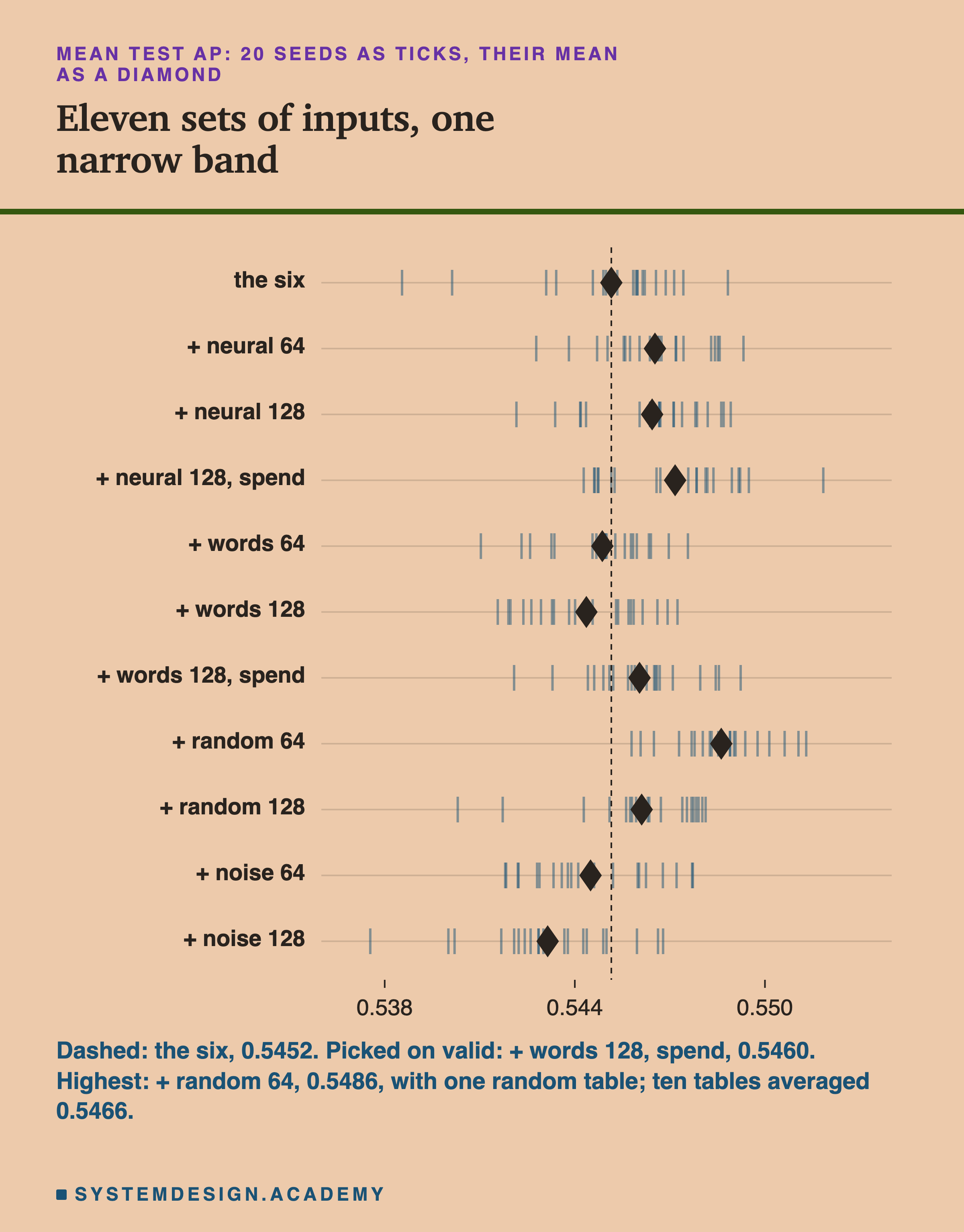
Here is every set of inputs with the six, scored on the five test months and averaged over 20 training seeds.
| inputs | columns | test AP | ROC-AUC |
|---|---|---|---|
| the six alone | 6 | 0.5452 | 0.798 |
| + neural 64 | 70 | 0.5465 | 0.799 |
| + neural 128 | 134 | 0.5464 | 0.799 |
| + neural 128, spend | 134 | 0.5472 | 0.799 |
| + words 64 |
How Sure Can I Be?
Gaps of a few thousandths need care. I checked two kinds of luck.
Luck in training. The model sets aside 10 percent of the train rows at random to decide when to stop adding trees. This is called early stopping, and the seed moves it. So every set of inputs was trained with 20 seeds, 0 to 19. The six alone ranged from 0.5385 to 0.5488 over the seeds. That spread is larger than any gain in the table.
Luck in which customers were tested. A bootstrap draws the test customers again at random, with repeats allowed, within each test month. I did that 1,000 times, with the same draws for every set of inputs. Each time I worked out the 20-seed mean AP of each one minus the six. The middle 95 percent of those gaps is the 95% interval.
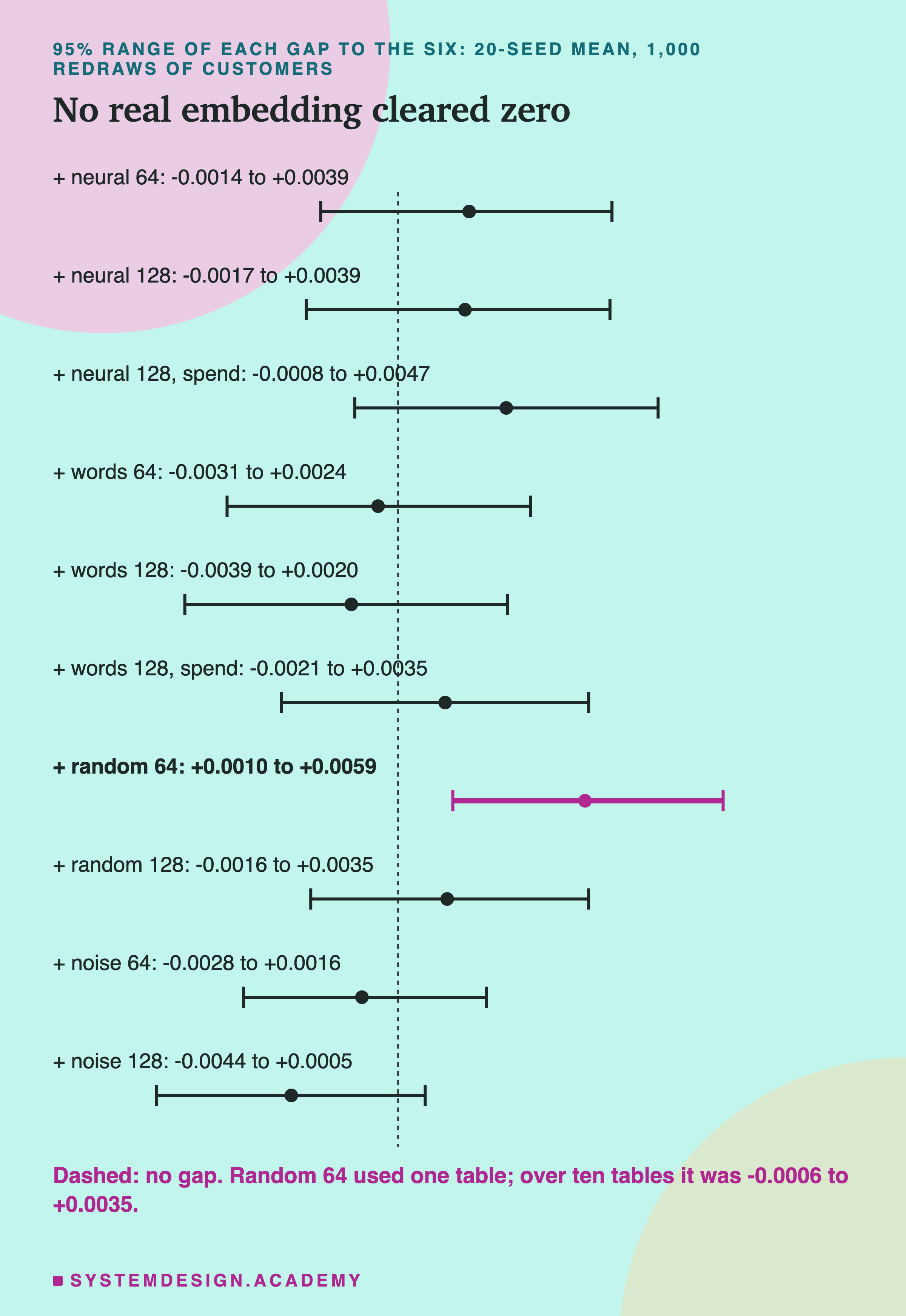
Every real block crossed zero. The neural model at 128 numbers: -0.0017 to +0.0039. The pick, word counts at 128 with spend: -0.0021 to +0.0035. None of them can be told apart from the six.
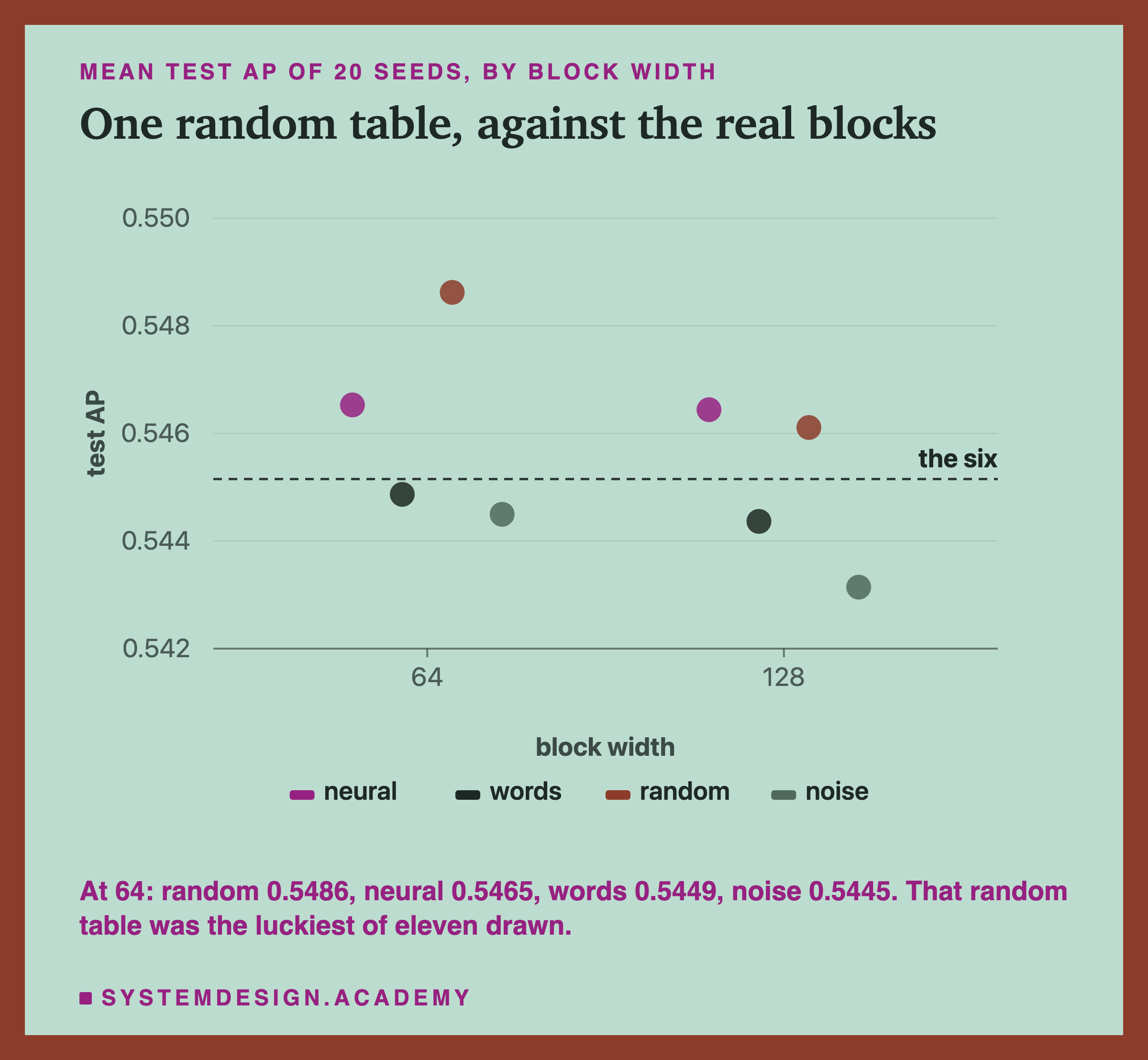
Only one interval sat clear of zero: random directions at 64, +0.0010 to +0.0059, above the six in all 5 test months. An independent review then retrained it with five other random tables, and found mine the luckiest.
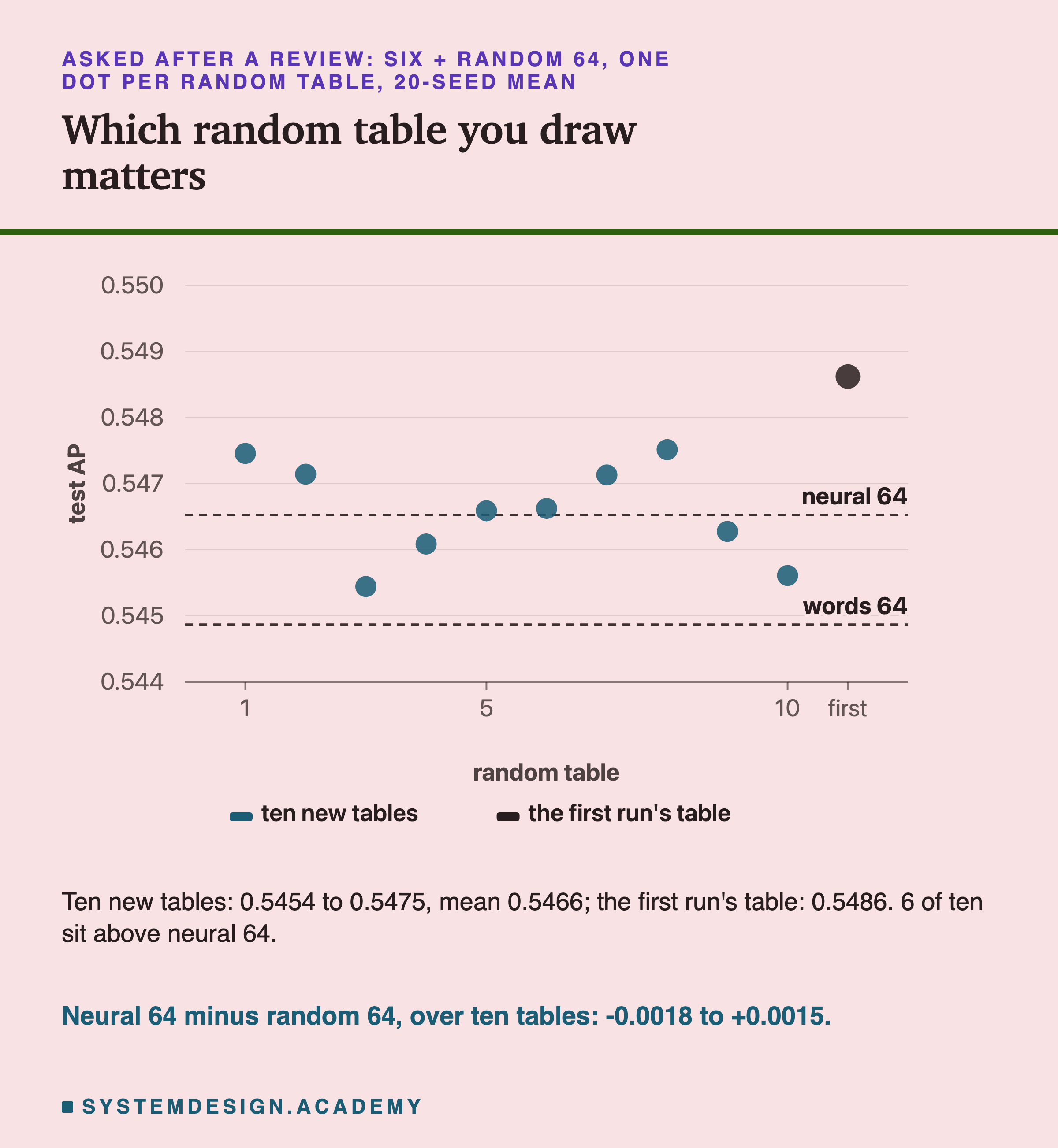
So, after the review, I drew ten new random tables, with the design written into the lab's docstring before it ran. Over all ten, random 64 against the six was -0.0006 to +0.0035, which crosses zero. The one clear interval came from one lucky draw of the random table, the same mistake as reading one shuffle as a finding. What survives is narrower: a block with no meaning at all did as well as the blocks with meaning.
Meaning Against Random Directions
The fair question is not "did the six plus a block beat the six". A block adds columns, and the columns alone could matter. The fair question is whether a block with meaning beats a block of the same width without it.
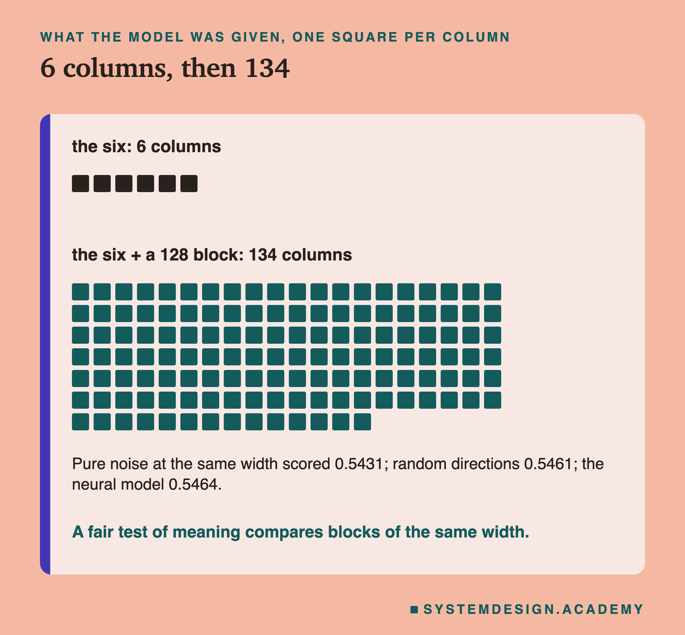
So the design put each real block against random directions of the same width. With the first random table alone, random 64 seemed to beat both real 64 blocks. Neural minus random was -0.0042 to -0.0001, and words minus random -0.0058 to -0.0016. That rested on one draw of the table.
After the review I drew ten new random tables and ten new noise draws. I retrained every random and noise contestant on each one with 20 seeds, and bootstrapped the mean over all 200 fits. These intervals were added after the results, and are labelled so:
| real minus random, ten tables | 95% interval |
|---|---|
| neural 64 | -0.0018 to +0.0015 |
| words 64 | -0.0036 to +0.0001 |
| neural 128 | -0.0006 to +0.0027 |
| words 128 | -0.0026 to +0.0006 |
Every interval crosses zero. No real beat random directions at either width, and random directions did not beat them either. Random directions did as well as either embedding; how far ahead they look depends on which random table you draw.
The Blocks on Their Own
A block that adds nothing to the six could still carry signal of its own. Maybe the six already know it. So the design also trained each 128 block with no six at all.
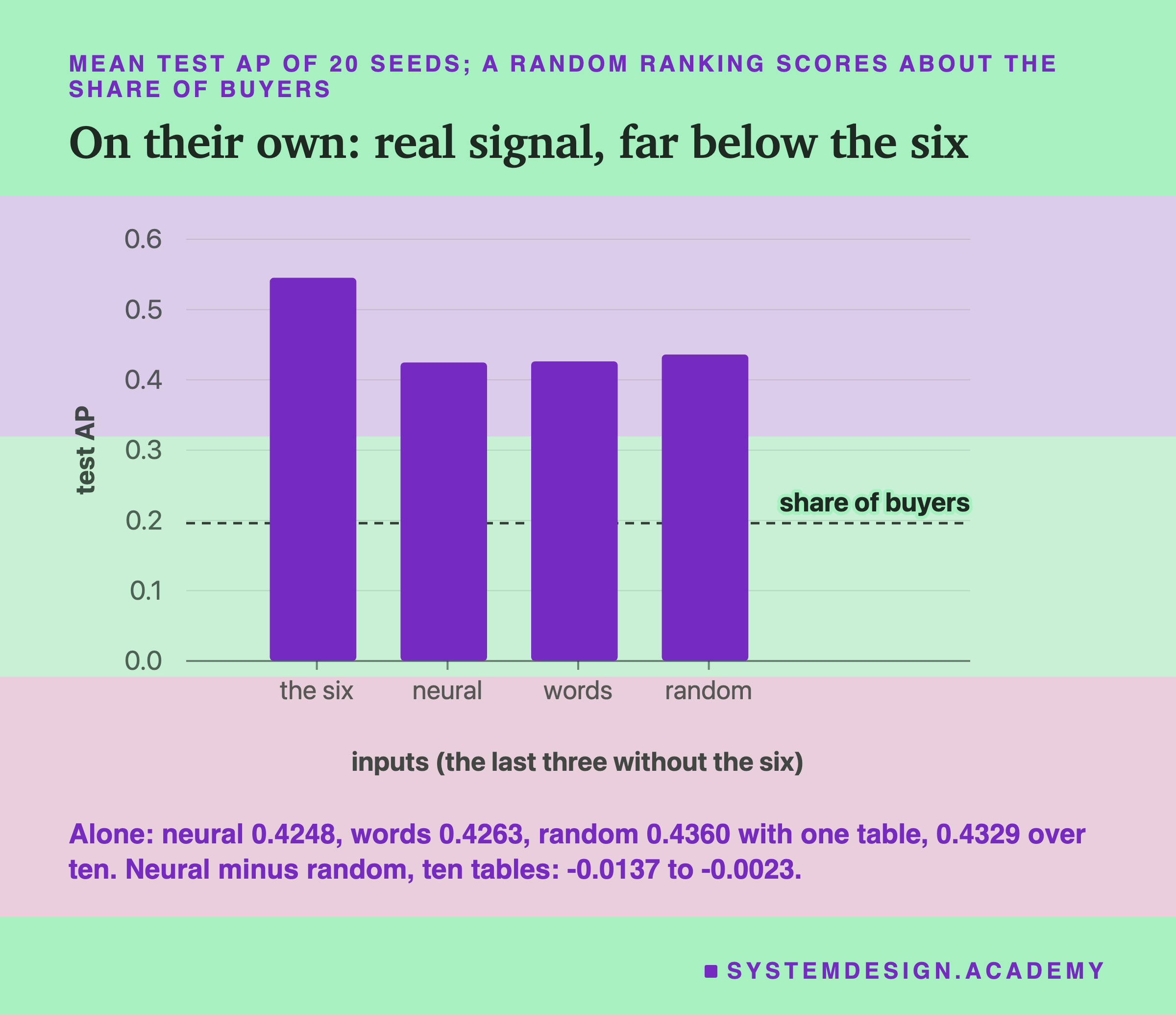
All three blocks carry real signal on their own: they score about 0.43, far above the 0.196 of a random list. A customer's products say something about whether they come back. But all three are far below the six at 0.5452, and the six already hold most of what the blocks know.
Here the random block came out on top, and the ten tables held it up. Over ten tables, the neural block alone minus random was -0.0137 to -0.0023 at 128, and -0.0163 to -0.0040 at 64. Word counts alone minus random was -0.0121 to -0.0015 at 128, and -0.0117 to +0.0011 at 64, which crosses zero. With the first single table, the two 128 gaps had been -0.0188 to -0.0041 and -0.0171 to -0.0030. All ten random tables scored above both real 128 blocks alone.
So the result is not just "the six already had it". On their own, a mean of the neural vectors told the model less than a mean of random ones. With the six, the two could not be told apart.
Why Would Random Do as Well? A Check After the Results
Everything on this slide was designed after I had seen the main results. Its design was written into the lab's docstring before it ran, and it trains no model.
My idea: product names that mean similar things get similar vectors. In this shop most products are gifts and home decorations, so many vectors point roughly the same way. A mean over 30 or more of them gets pulled toward one common direction, and customers end up looking alike. Random directions sit almost at right angles to each other, so a mean of them keeps more of which products went in.
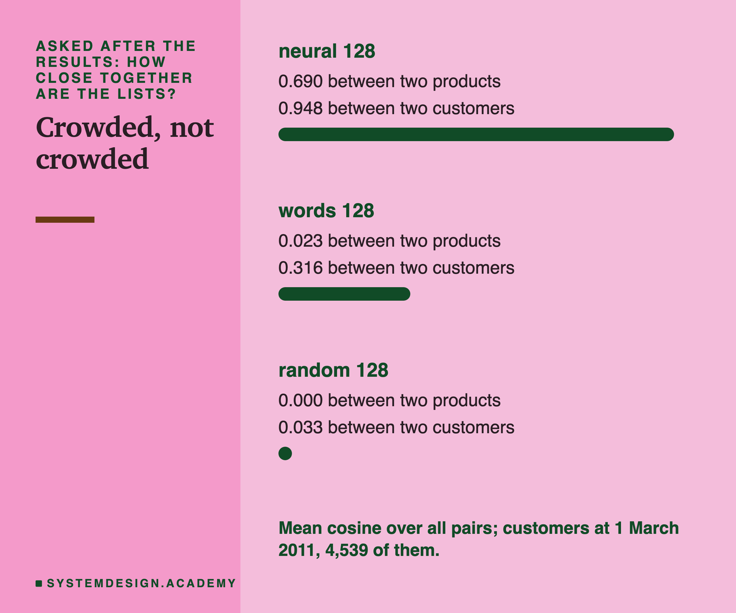
The numbers fit the idea for the neural model. Two of its product vectors had a mean cosine of 0.690, so they mostly point one way. Two customers' mean vectors at 1 March 2011 had a mean cosine of 0.948: nearly the same direction. For random directions those numbers were 0.000 and 0.033.
But the numbers do not fit for word counts. Its product vectors were barely alike, 0.023, and two customers only 0.316. Yet at 128, word counts alone also lost to random directions alone, by about as much as the neural model did. So crowding cannot be the whole story.
There is also a reason to doubt crowding matters at all. A tree model cuts each column at its own values, into at most 255 steps. Values packed close together are spread over those steps just the same. So the cause is not pinned down. Crowding describes the vectors; it does not show that crowding is what cost the score.
The Pick, and the Seed That Lied
Two smaller lessons came out of the run, both about how easy it is to fool yourself.
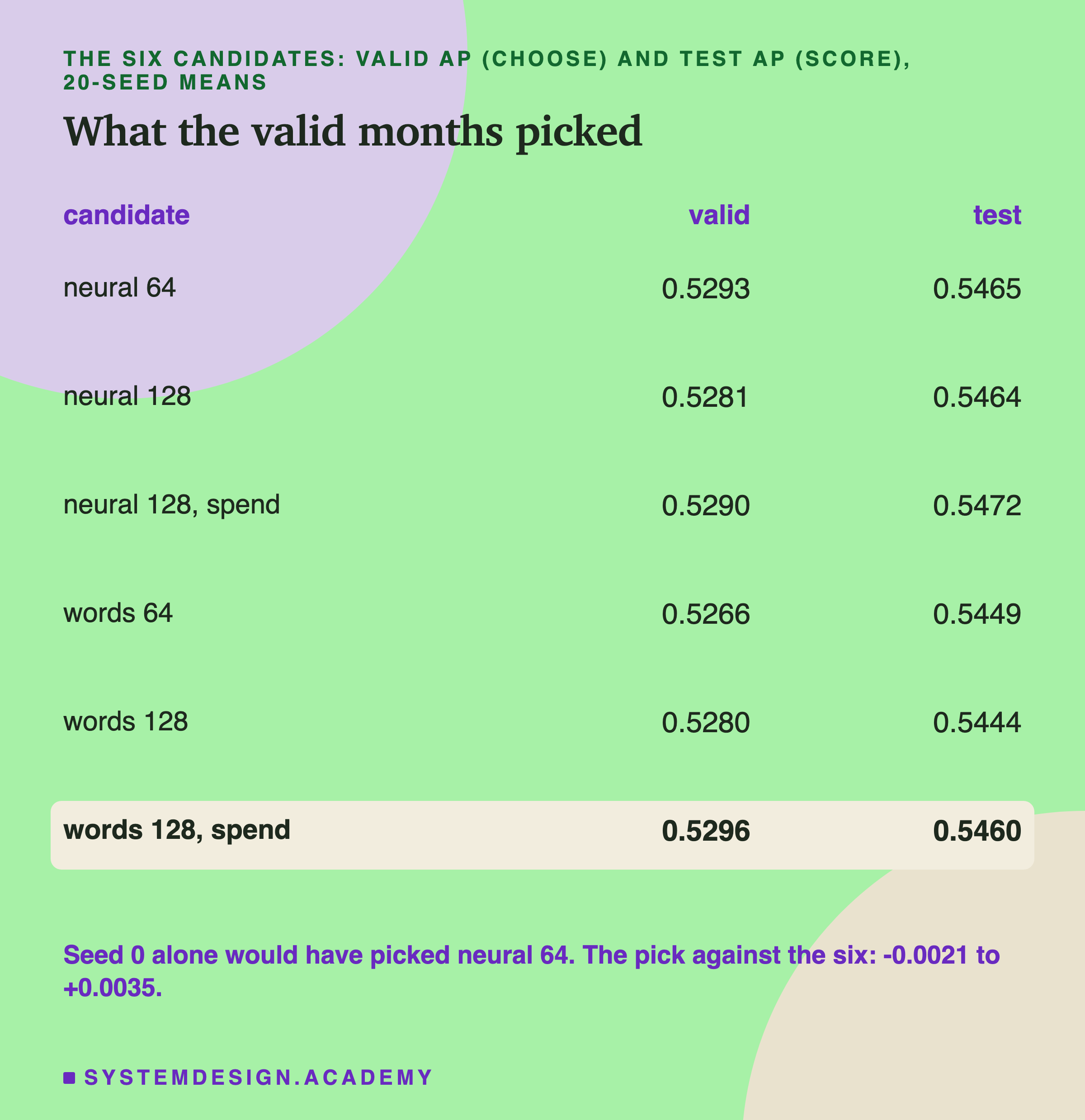
The pick. The valid months chose word counts at 128 with spend weights, at 0.5296. The next two were within 0.0007 of it. With seed 0 alone, the valid months would have chosen the neural model at 64. Either way, the picked block could not be told apart from the six on the test months.
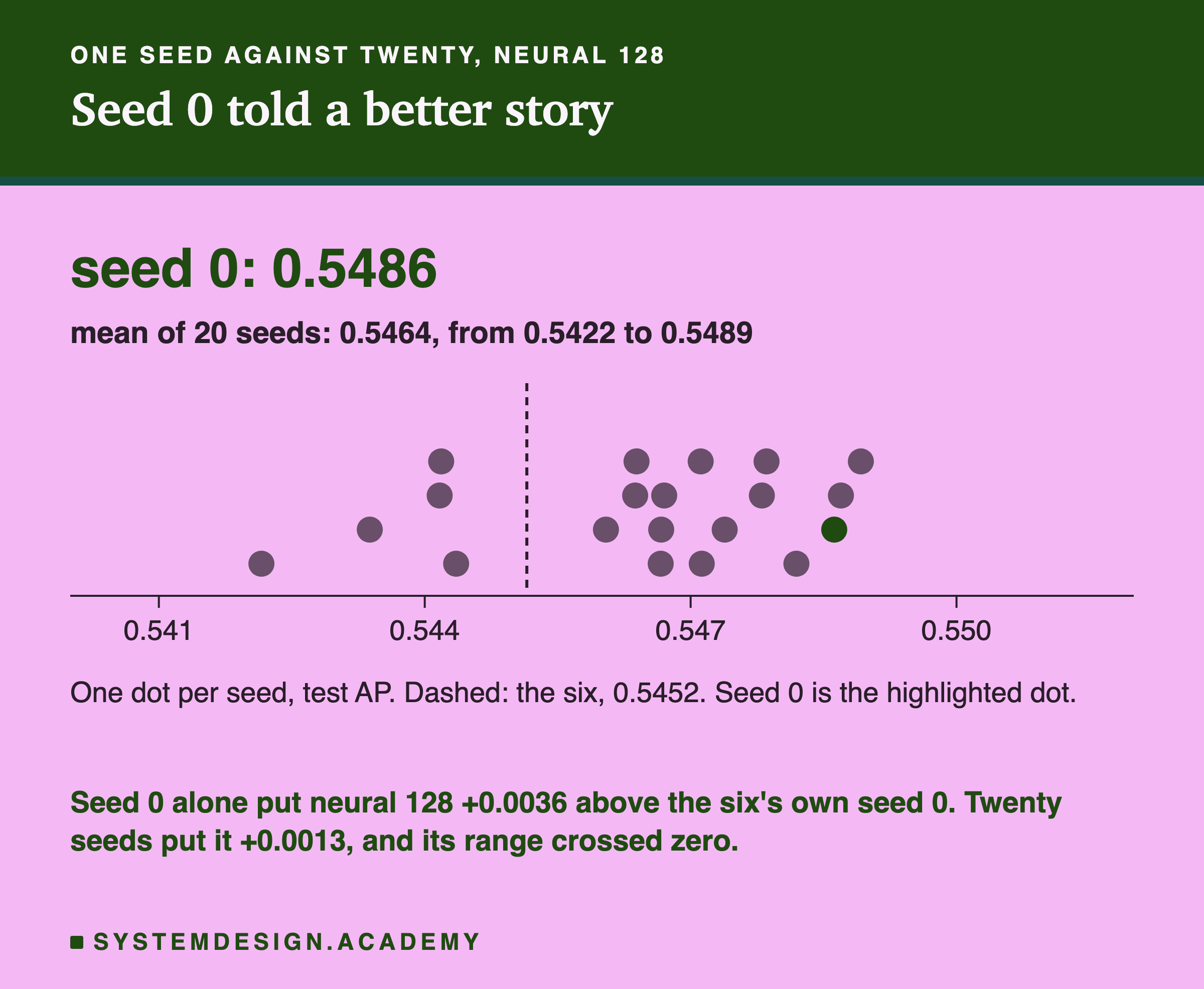
The seed. Suppose I had trained the neural block at 128 with seed 0 only. I would have seen 0.5486 against 0.5450 for the six at seed 0. That is a gain of +0.0036, from the third best seed of the twenty. Over 20 seeds the gain shrank to +0.0013, and the interval crossed zero. One seed is one draw. The chapter has learned this the hard way more than once, and it would have fooled me here too.
What a Block Costs
Even if a block helped, it would not be free. Here is what this one costs.
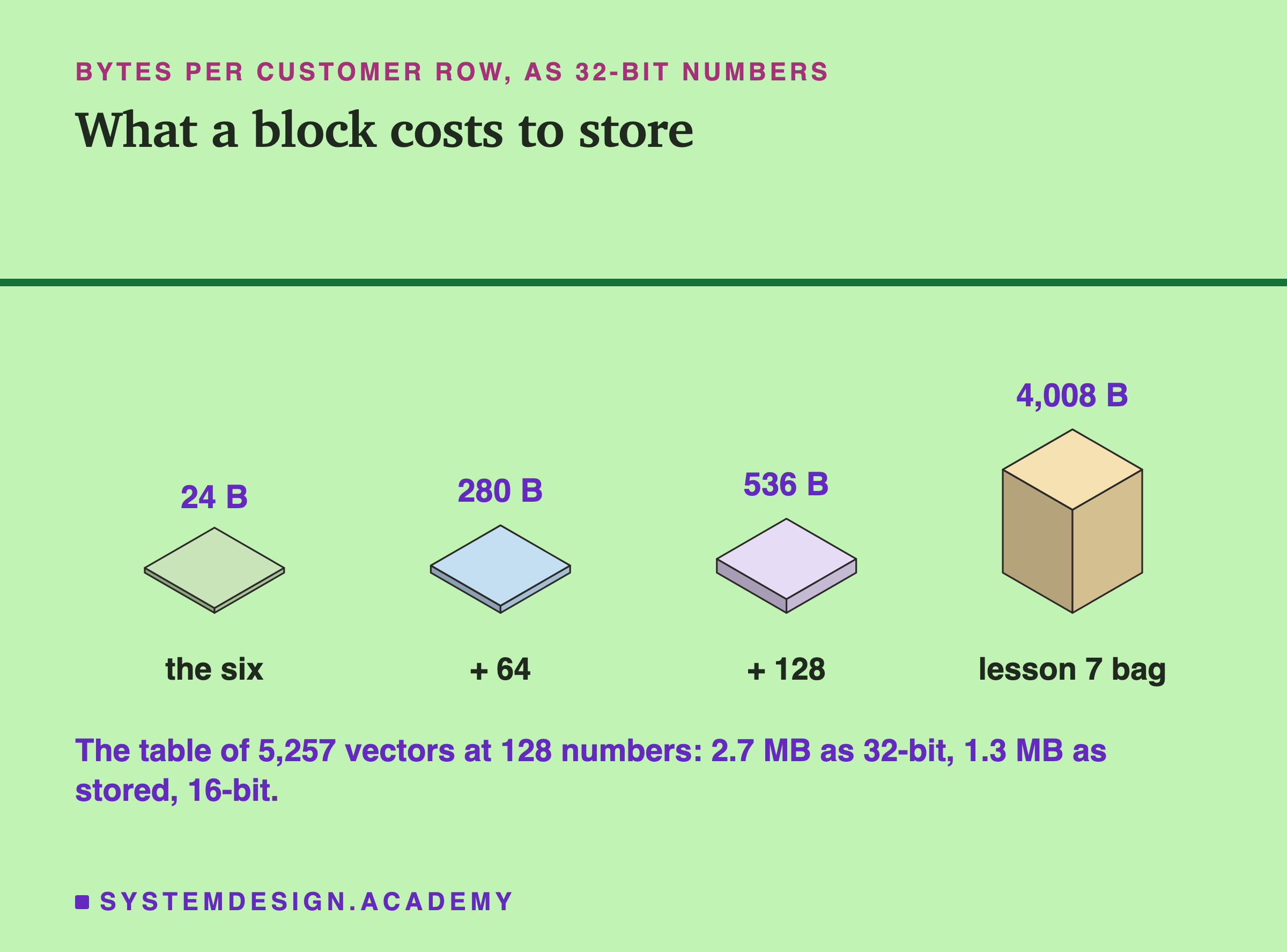
Per customer. A 128 block adds 512 bytes per row as 32-bit numbers, against 24 for the six. The training table the model gets, in 64-bit numbers, grew from 2.1 MB to 47.7 MB.
The vector table. 5,257 vectors of 128 numbers are 2.7 MB as 32-bit numbers, or 1.3 MB as I stored them. That is small. It is also a one-off cost: 83 calls to Ollama, 50,258 tokens. I give no time for it. Ollama and the laptop were shared with other work while it ran, so any seconds would be unfair.
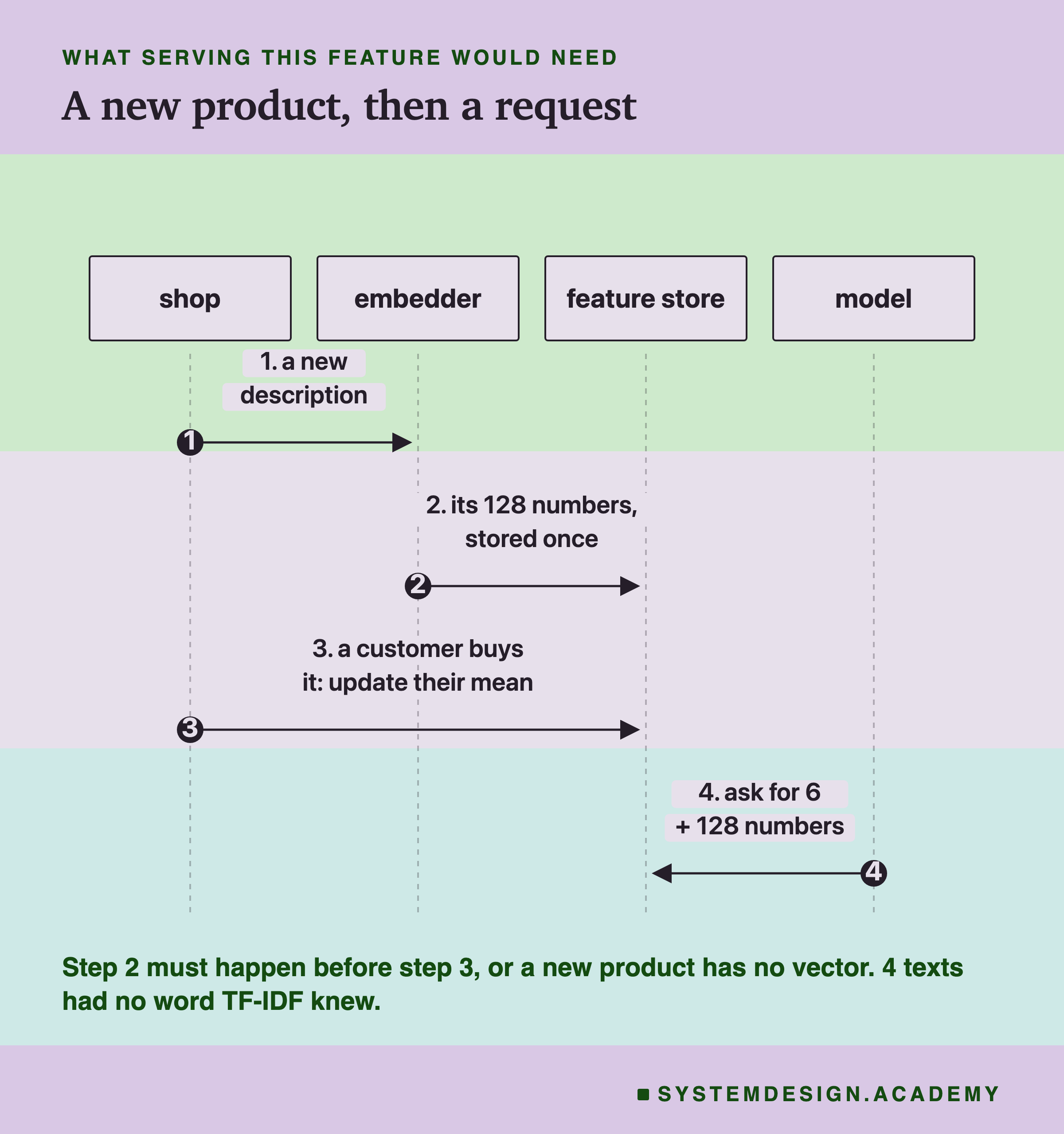
At serving time. The real cost is in the moving parts. A new product needs its vector before any customer's mean can include it, so an embedding job must run before the updates the customer. If the embedding model ever changes, every vector and every customer mean must be rebuilt, which is the versioning problem of an earlier lesson in a new form. For word counts there is a quieter trap: a product whose words were all unseen gets a vector of zeros. Four texts here had that.
The Lab's Code, Piece by Piece
The lab is one file, scripts/labs/features/embeddings_features.py. It imports lesson 1's feature code for the six, so they are built exactly as before. Its base contestant must reproduce lesson 1's score of 0.5450 at seed 0, to twelve decimal places, or the run stops. It did.
build_vectors embeds each distinct description once. It sends batches of 64 texts to Ollama's /api/embed, each with the "classification: " prefix, and keeps the 768 numbers in a file outside the repository. matryoshka does the card's resize: layer norm, keep the first 64 or 128, divide by the length. For word counts it fits TfidfVectorizer() and TruncatedSVD(n_components=k, random_state=0) on the texts from before March 2011 only. The four tables are saved, rounded to 16 bits, in results/emb-vectors.npz. If that file exists, nothing is embedded at all.
load_tables reads that file and adds the random directions: one fixed list of normal random numbers per description, from numpy.random.default_rng(7), each divided by its length. After the review, multi draws ten more tables from default_rng(1000 + k) and ten noise draws from default_rng(2000 + k). It retrains every random and noise contestant on each, and bootstraps the mean over all 200 fits per contestant.
Try It Yourself
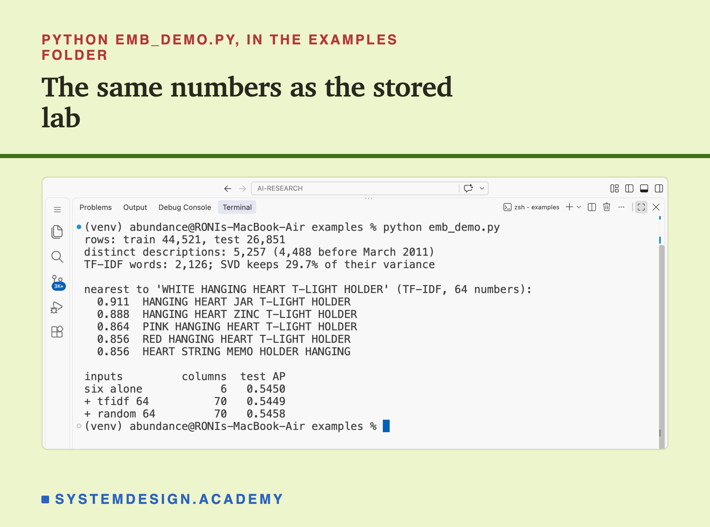
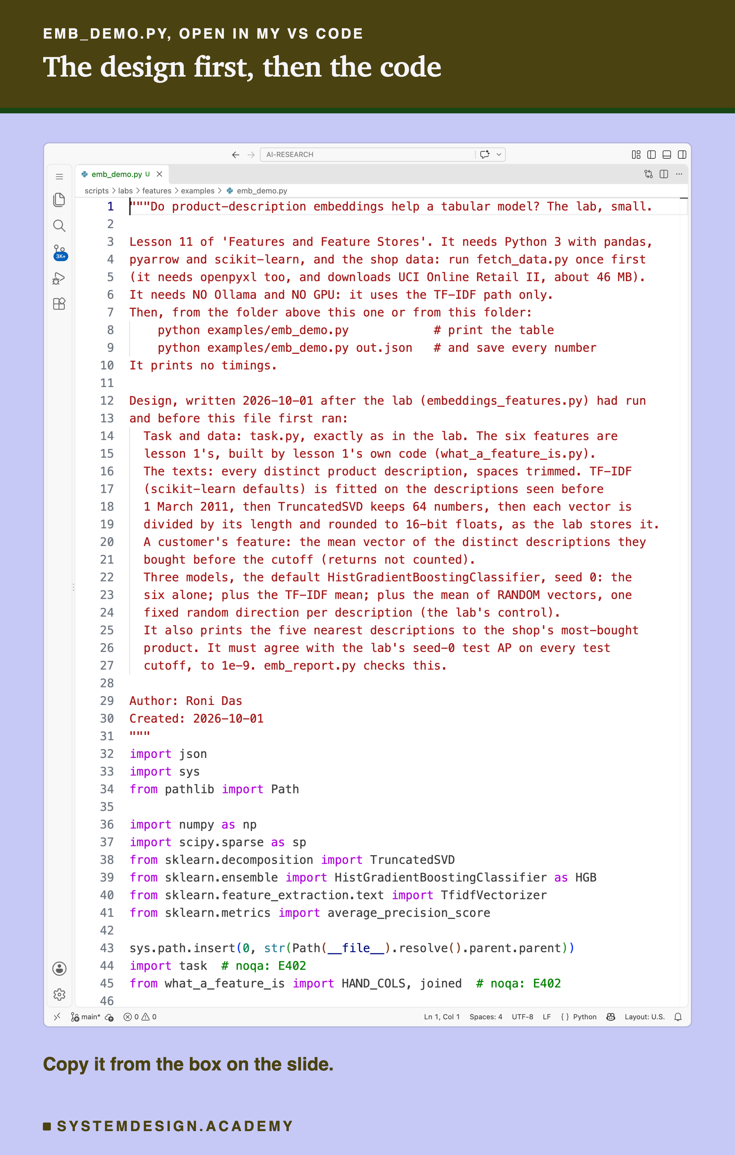
The full lab trains 280 models, plus 1,780 more for the check after the review, and needs Ollama. I wrote a small demo that needs neither: it uses the word-count path only. It builds every customer's mean of TF-IDF vectors at 64 numbers, and of random directions, then trains three models at seed 0 and prints their test AP.
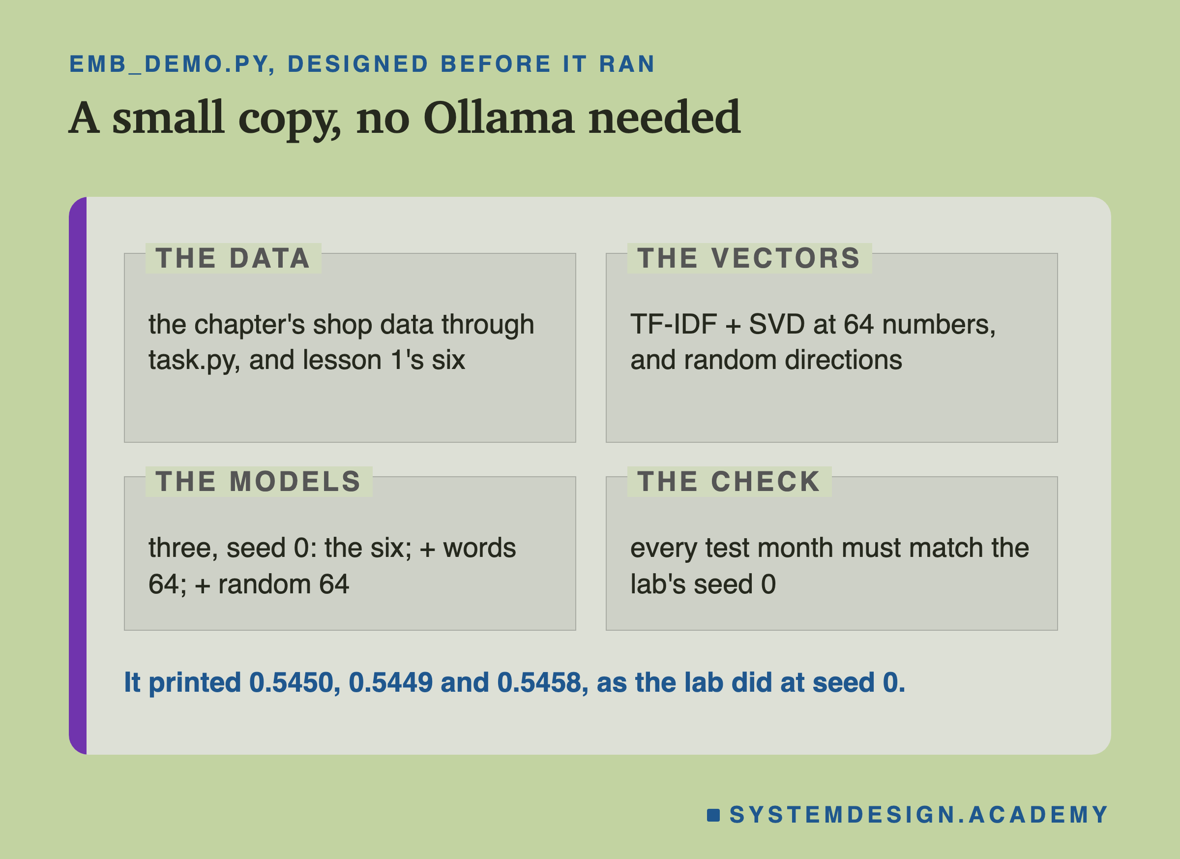
I wrote the demo's design into its docstring after the lab had run and before the demo first ran.
Before you run this lab. The full lab uses nomic-embed-text, running in Ollama on your own computer. The demo on this slide does not need it. If you want to run the full lab and have not set Ollama up yet, the lab setup guide shows how to install Ollama, download the model and check that everything works, on macOS, Windows or Linux. You can use a different model instead: the guide shows the one line to change, and your numbers will differ from the ones in this lesson.
For the demo you need Python 3 with pandas, pyarrow and scikit-learn: pip install pandas pyarrow scikit-learn openpyxl. First run python fetch_data.py from the scripts/labs/features folder. It downloads the shop data once, about 46 MB, and writes one cleaned file. Then run the demo. It needs no GPU. I ran it with scikit-learn 1.9.1 on a Mac. These libraries run on Windows and Linux too, but I have not checked the numbers there. Give it a file name, python emb_demo.py out.json, and it also saves every number. That is how was made.
Find a Product's Neighbours Yourself
This box holds the 400 real descriptions bought on the most lines before March 2011. It also holds TF-IDF with scikit-learn's default settings, written in plain Python, so it runs in your browser. The report checked that it gives exactly scikit-learn's numbers on these 400 texts.
Press Run to see the five descriptions nearest to the white hanging heart t-light holder. It also counts how many of the others share no word with it at all. For TF-IDF those get a cosine of exactly 0, however close their meaning: 321 of the 399. Then change MINE to any description in the list, such as "REGENCY CAKESTAND 3 TIER", and run again.
At the bottom it prints each set of inputs' real mean test AP over 20 seeds from the lab. So you can set what the vectors find next to what they did, or did not do, for the score.
Common Mistakes, and When Embeddings Help
No same-width control. Adding 128 columns can move a score with no meaning in them at all. Always compare against random directions and pure noise of the same width. Here, over ten random tables, random directions were never beaten by a real at either width. And draw several random tables, not one: the first one I drew was the luckiest of eleven.
Trusting one seed. At seed 0 the neural block looked like a gain of +0.0036. Over 20 seeds it was +0.0013, and the interval crossed zero.
Fitting the text model on the future. Fit TF-IDF and SVD on texts from before training ends, as here. A pretrained neural model learned from other text, not from your labels, so it reads no future label; but it can still change version, and every vector with it.
Embedding the same text again and again. Cache by text. Here 5,257 texts covered every line of two years of invoices.
When embeddings may help. When the text is the main thing you know about an item, for example a new product with no sales yet, where a code or a random direction has nothing to go on. When the model can use each item's vector directly, rather than a blurred mean. Or when the task is about the content itself, such as search or grouping. I did not test any of these here.
When to skip them. On evidence like this lesson's, when strong behaviour features already exist, as the six do here, and the question is about behaviour, such as whether someone comes back.
What This Lab Cannot Tell You
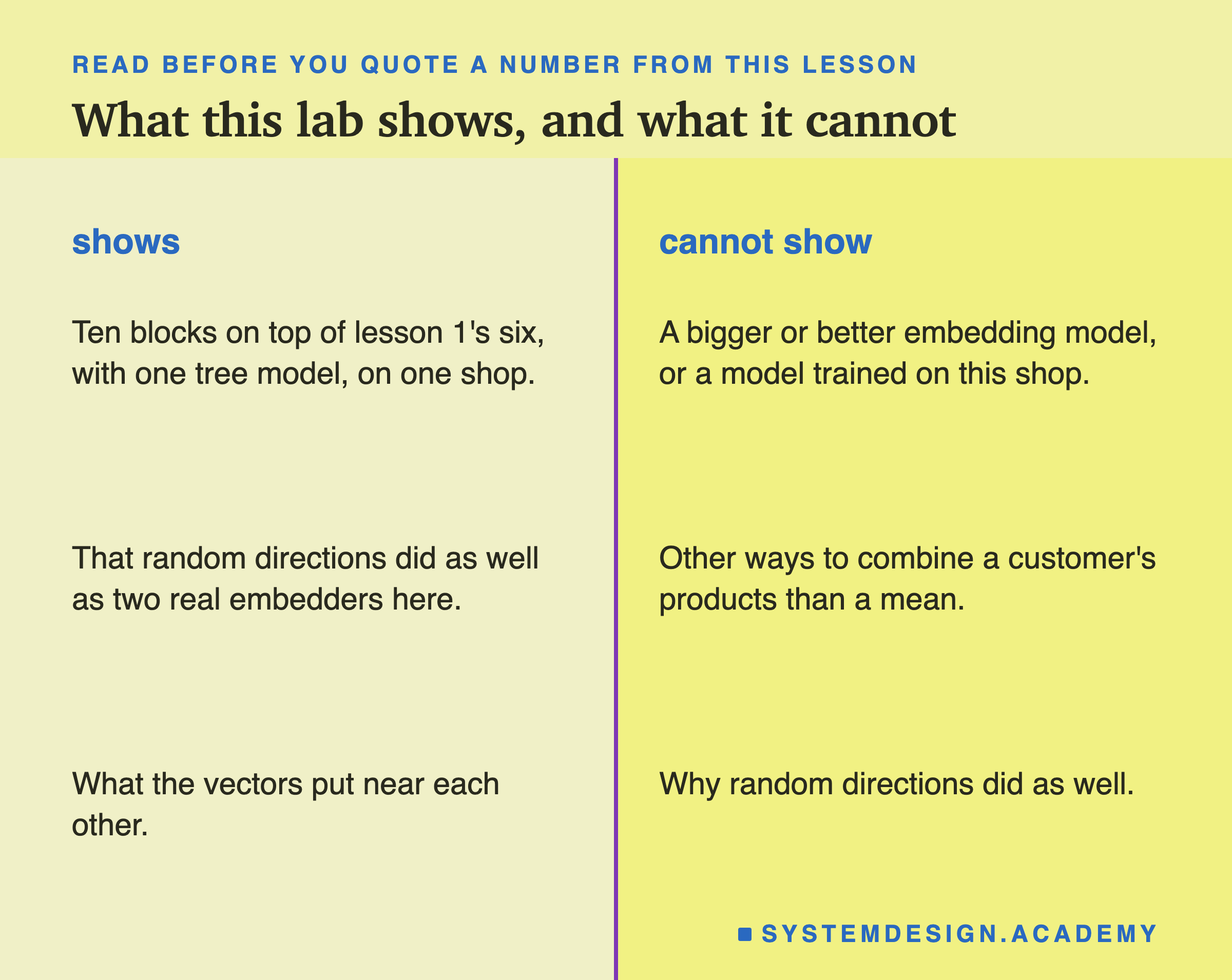
One shop, one task, one model. A tree model with default settings, on a 30-day buying question, with one small model and one word-count method. A larger model, a model trained on this shop's own data, or a linear model might behave differently. I did not test them.
One way to combine. I took a plain mean, and a spend-weighted one. A mean of 94 products looks like none of them, as customer 12349 showed. Other ways, such as the most recent products only, or one vector per product group, could keep more. I did not build them.
One check after the results. The crowding check is labelled on its own slide, and its design was written down before it ran. It describes the vectors; it does not explain the score.
No timings. The laptop and Ollama were shared, so I report counts and bytes only.
What to Do on Monday
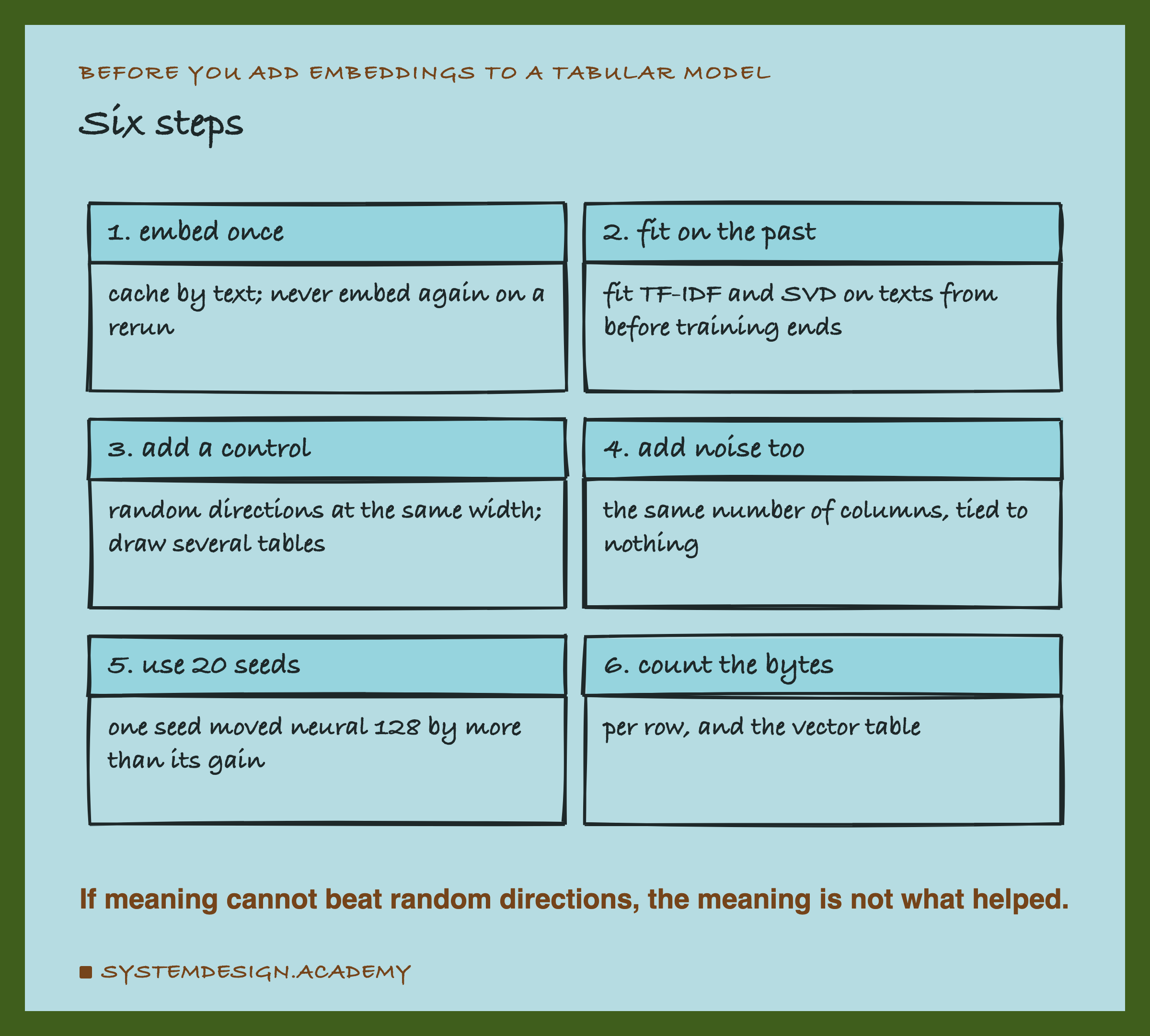
These are the steps I would take the next time someone says "let's add ".
-
Embed once, and cache by text. It is cheap to store and expensive to repeat.
-
Fit anything fitted on the past only. TF-IDF and SVD here saw only texts from before March 2011.
-
Build random-direction controls of the same width, and draw several tables. It is three lines of code. Here one table seemed to beat both real embedders at 64 numbers; ten tables showed that was a lucky draw.
-
Add pure noise too, to see what extra columns alone do.
-
Use 20 seeds and an interval. One seed showed a gain of +0.0036 that was not there.
-
Count the bytes, per row and for the vector table, before you put it in a .
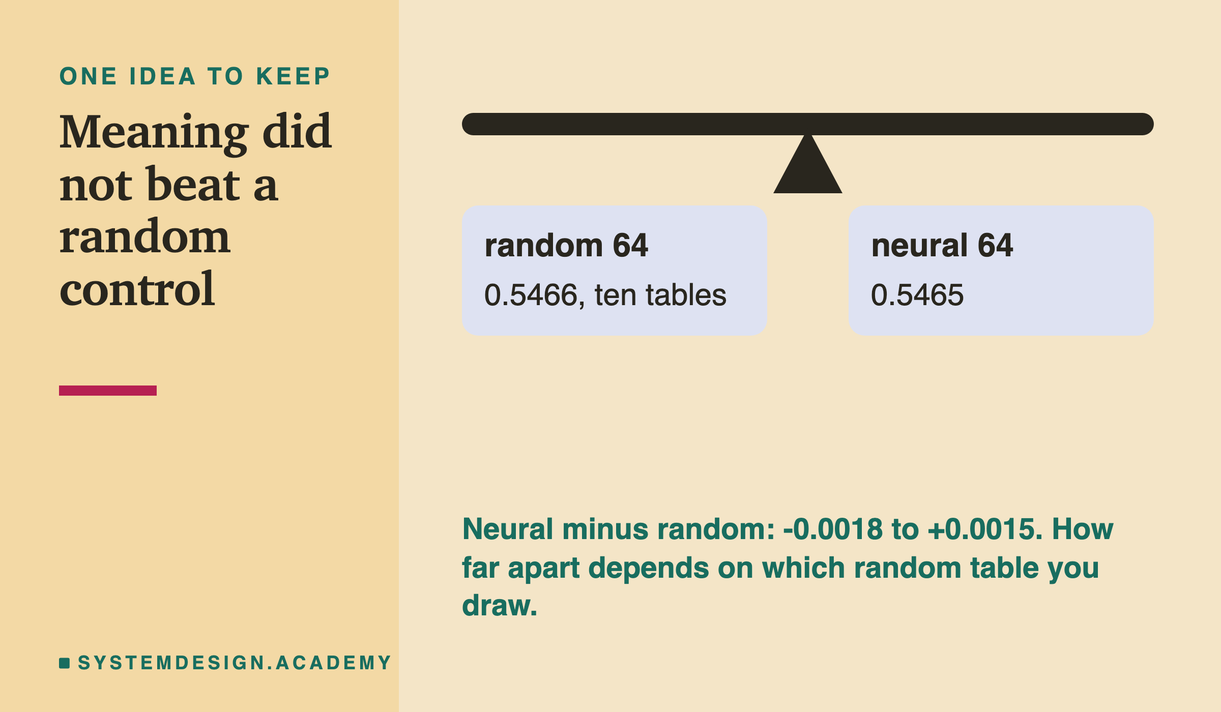
The one idea to keep: on this shop, the vectors grouped products by meaning very well, and the model did not need it. Which products a customer bought helped a little over pure-noise columns; what those products were called did not add anything I could measure. Random directions did as well as either embedding, and how far ahead they look depends on which random table you draw.
Knowledge Check
Knowledge Check
4 questions - Score 80% to pass
Why did the lab add a block of random directions, one fixed random list per description?
The neural block at 128 numbers scored +0.0036 over the six at seed 0. What did 20 seeds show?
For the assorted colour bird ornament, how did the two real embedders' neighbours differ?
Why should a gain from 128 extra columns be compared with noise and random directions of the same width?