Let me start with a party.

You are hosting a big party, and you want every guest to get a small card with their name and a short note on it. You can do this in two ways.

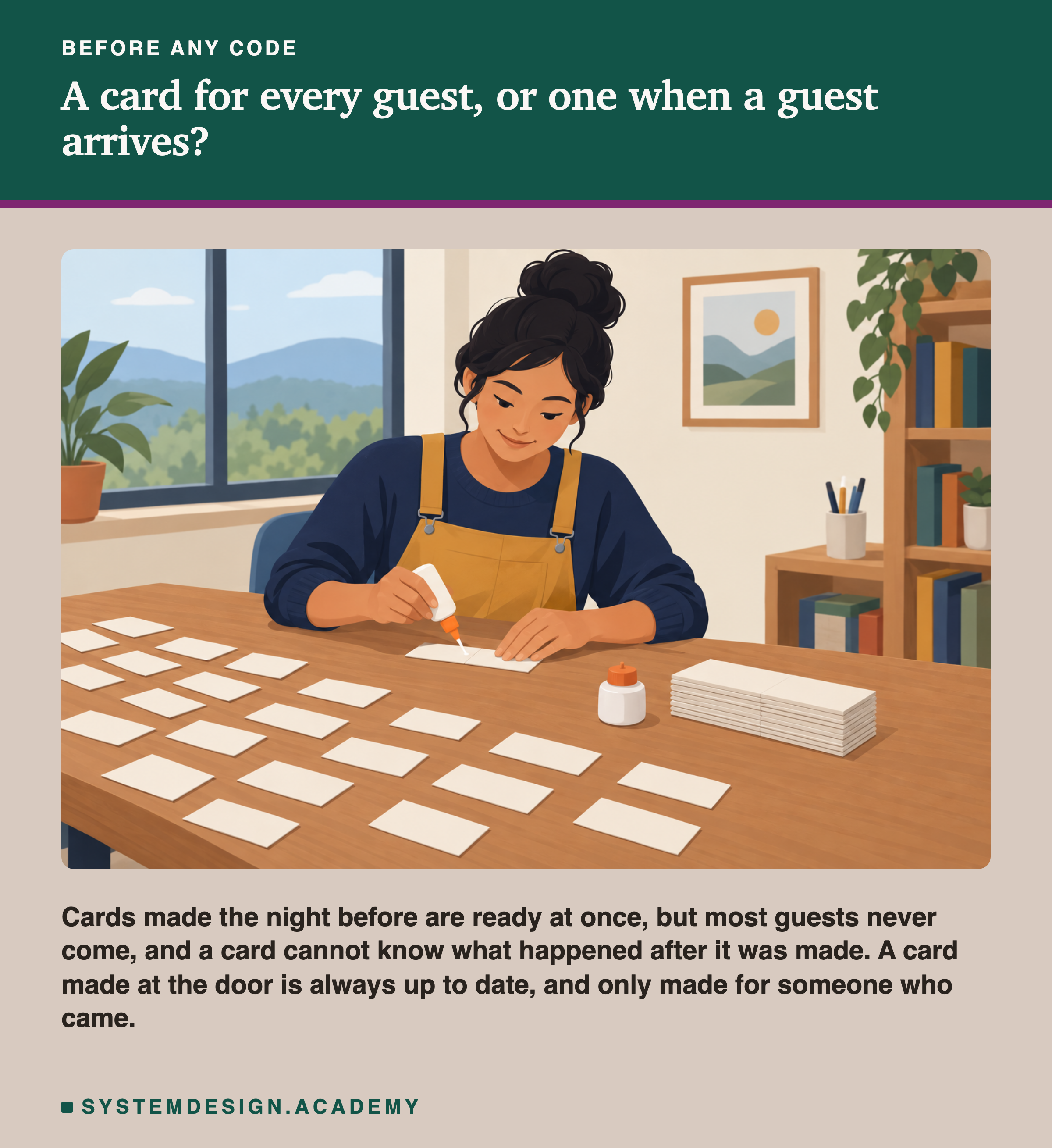
The first way is the one in the picture. The night before, you sit down and write a card for every person on your list. When a guest walks in, you hand over their card at once. It is fast at the door. But you wrote many cards for people who never came. And if a guest told you some news this morning, the card does not know it, because you wrote it last night.

The second way is to write each card at the door, when the guest arrives. Every card is up to date, and you never write a card nobody uses. But each guest waits a moment while you write, and you must be at the door the whole evening.

A machine learning model that gives each customer a number faces the same choice. In this lesson I measure both ways on a real shop.

This is the first lesson of a new chapter about serving a model: running a trained model so that other programs can ask it questions and get answers.

The model is the one from the features chapter. If it is new to you, please read what a feature is first. In short: a real online shop in the UK sold gifts, mostly to other shops, from 2009 to 2011. For each customer, the model looks at six numbers made from their past orders. Two examples are the days since their last order and how many orders they made. Then it guesses how likely they are to buy again in the next 30 days.

The survey lesson on model serving already explains, in words, the two main ways to serve a model. In batch serving, a job scores many rows on a schedule. In online serving, each request is scored as it comes. It says the main question is whether someone is waiting for the answer. I will not repeat it. Here I measure a different part of the choice: how much an old stored answer costs, how much work a batch wastes, and who it misses.

Two earlier lessons measured something close. Feature freshness found that features up to 14 days old cost nothing measurable on this same shop. And batch vs streaming data found that fresh counts cut the error almost in half for bike rentals in the next hour. This lesson sits between them.

Please read this slide slowly if any word is new. Every slide after it uses these words.

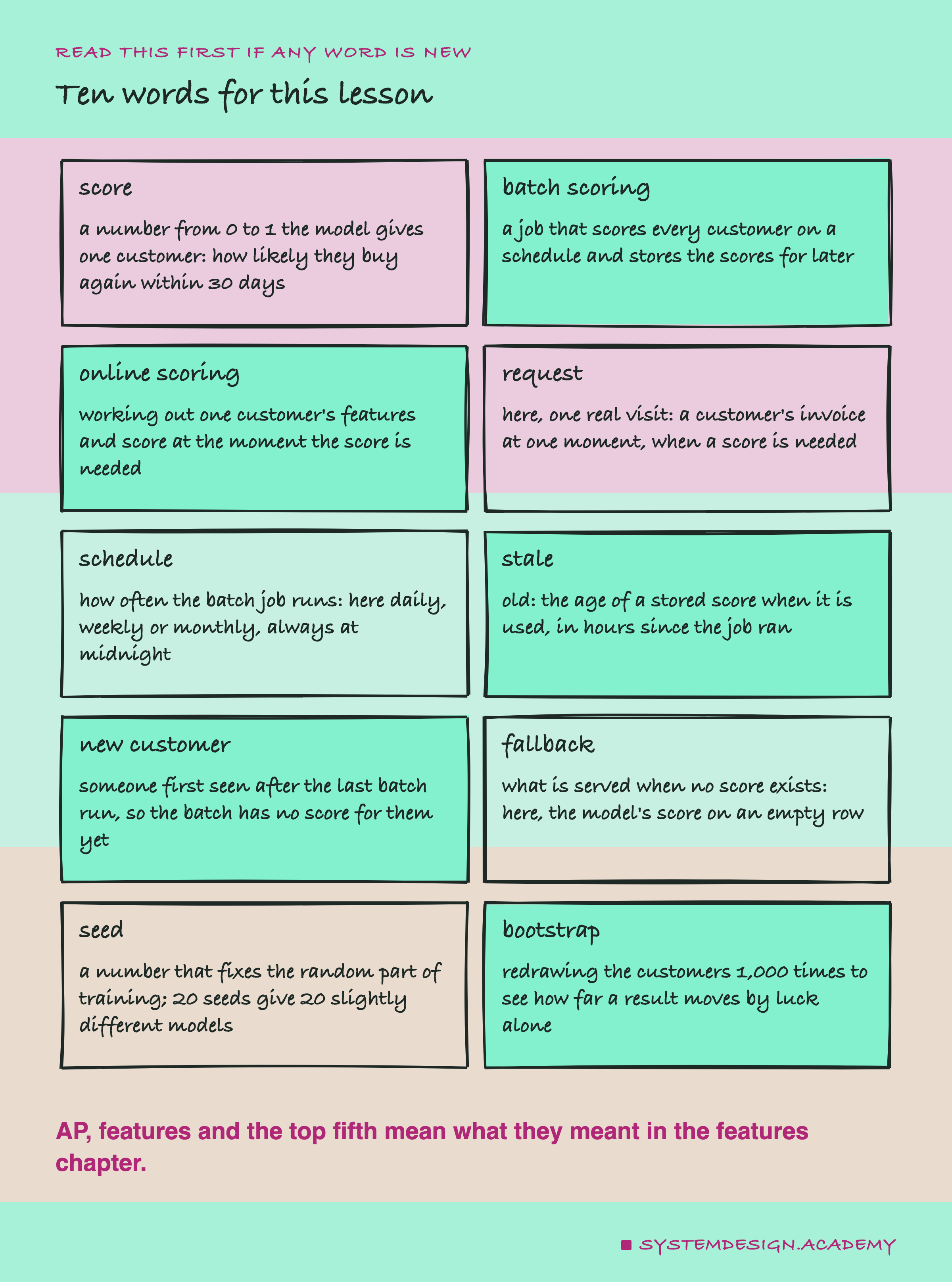
A score is the model's answer for one customer: a number between 0 and 1. A higher score means the model thinks the customer is more likely to buy again within 30 days.

Batch scoring is like writing all the cards the night before. A job wakes up on a schedule, for example every night at midnight. It gives a score to every customer the shop knows, and stores the scores in a table. Later, when the shop needs a score, it looks it up. Online scoring is like writing the card at the door. When the shop needs a score, it works out the customer's six numbers right then, from everything that has happened so far, and asks the model.

A request is one moment when the shop needs a score. Here it is a real visit: one invoice from a customer. Most invoices are orders, but returns count too: 1,158 of the 7,403 visits (15.6%, about 1 in 6) were return-only invoices, and 22 mixed returns and purchases. A stored score is stale when it is old. I measure how stale it is in hours, from the moment the job ran to the moment the score was used.

AP, average precision, is the score from the features chapter. It goes from 0 to 1 and says how well the scores put the customers who did buy again above the ones who did not.

Here are the two ways side by side, for one real visit from the lab: customer 12362, who placed an order on 26 October 2011 at 13:47.

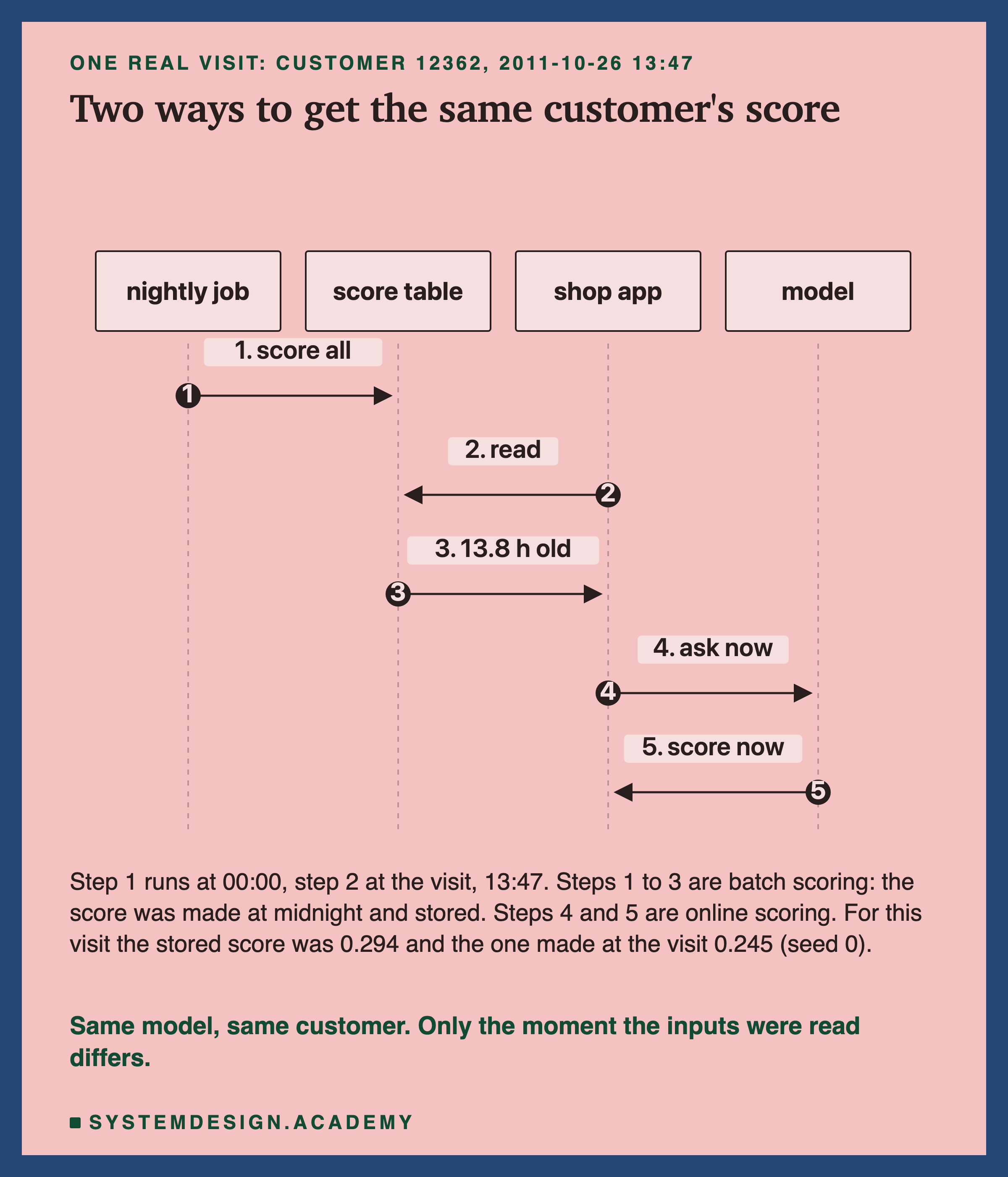
In the batch way, a job ran at midnight. It worked out the six numbers for this customer as they were at 00:00, asked the model, and stored the answer. At 13:47, when the visit came, the shop read that stored answer. It was 13.8 hours old.

In the online way, the shop works out the six numbers at 13:47, from every order before that moment, and asks the model right then.

Both ways use the same model, trained in the same way. The only difference is when the inputs were read. So the whole question of this lesson is this: does reading the inputs earlier make the answer worse, and by how much?

For this one visit, the two scores were 0.294 and 0.245. One visit cannot tell you which way is better. For that, I need thousands of visits.

This lesson leans on three facts about tools and data. I downloaded each source at a fixed version and found every quote in it word for word. They are in results/bo-factcheck.json, which the lab's fact-check mode wrote after the main run.

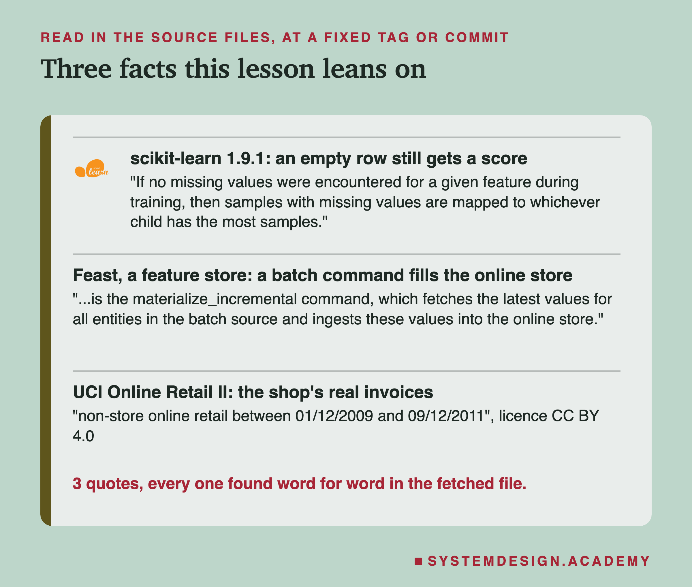
scikit-learn is the Python library the model comes from. Its documentation says what happens when a value is missing at prediction time, and the model never saw a missing value in training. The row goes to "whichever child has the most samples". So even a row with all six numbers missing gets a score. I use that as the fallback for customers the batch has no score for.

Feast is a feature store, a tool from the features chapter. Its documentation describes a command, materialize_incremental, that "fetches the latest values for all entities in the batch source and ingests these values into the online store." In plain words: a batch job copies fresh numbers into the fast store that serving reads. That is batch work feeding online serving, and it shows that real systems often mix the two.

The data is the UCI Online Retail II dataset, real invoices from a UK shop, shared under the CC BY 4.0 licence.

I wrote the lab's design into the docstring of scripts/labs/serving/batch_or_online.py before it first ran. Before that, I had read the features chapter's code and the names of the data's columns. I had not counted or scored any visit in the test months.

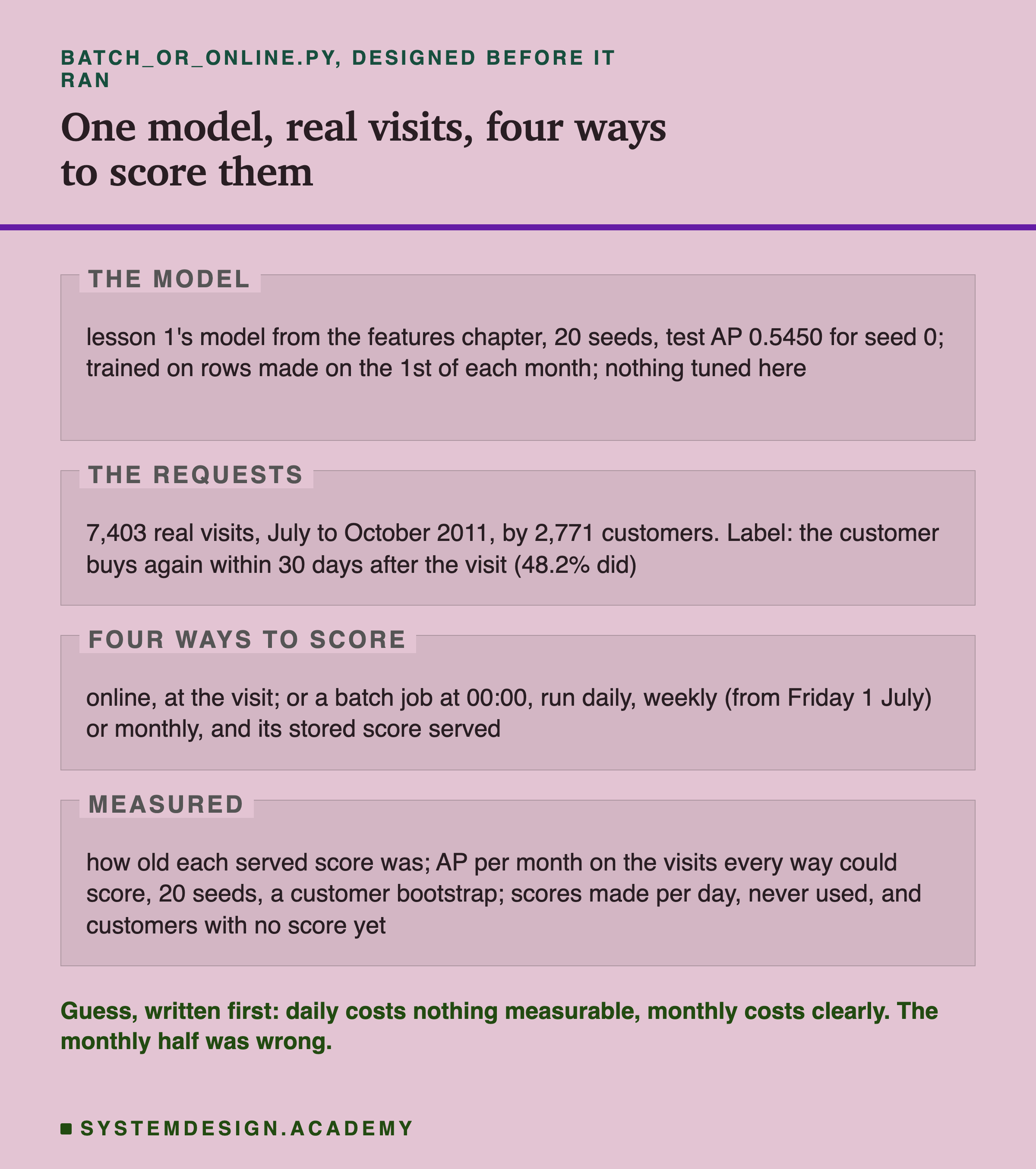
The model. The lab trains the features chapter's lesson 1 model 20 times, with seeds 0 to 19, on the same training rows. It stops unless every seed gives exactly the test AP that lesson stored; seed 0 gives 0.5450. Nothing is tuned or chosen in this lab.

The requests are real. Each request is a real moment from the shop's data: one customer's invoice at one time, between 1 July and 31 October 2011. Several invoice lines with the same time count as one request. That gave 7,403 requests from 2,771 customers.

The label. For a visit at time t, the label is 1 if the same customer makes another purchase after t and within 30 days. I left out the visit's own order, because counting it would make every label 1. This is the chapter's question, "will they buy in the next 30 days?", asked at the moment of the visit instead of on the 1st of the month.

Four ways to score each visit. Online: the six numbers worked out at the visit. Daily: a job at midnight every day, and the visit gets the score from the last midnight. Weekly: the same every 7 days from Friday 1 July. Monthly: the same on the 1st of each month. Every way uses the same trained models.

Before the results, two choices in the design matter a lot, so I want to explain them.

First, the same visits for every way. Some visits come from customers a batch has never scored.

A daily batch at midnight has no score for someone whose first order was at 09:00 today and who comes back at 15:00. If I let each way skip the visits it cannot score, the four ways would be graded on different visits, which is not fair. So the main comparison uses only the 6,613 visits that all three batches could score. I call it the common set. A second comparison uses every visit with any history, 6,787, and there a batch serves its fallback score for the visits it has no score for.

Second, how sure the result is. Training has a random part, so I trained 20 models with 20 seeds and report the mean. And which customers happened to visit is luck too. So the lab redraws the customers 1,000 times, keeping all of a customer's visits together in each month, and works out the 20-seed mean every time. This is a bootstrap. If the middle 95% of the redrawn differences crosses zero, I say the batch "cannot be told apart" from online. It does not mean the two are equal. It means this data cannot show a difference.

AP is worked out for each month, July to October, and then averaged, as the features chapter did for each month's cutoff.

The lab also checks its own feature code. At every one of 124 midnights, its six numbers for every customer were exactly equal to what the features chapter's own function gives. For 300 visits drawn at random, the visit-time numbers were exactly equal too.

This is a real recording of the report script, bo_report.py, on the laptop where the lab ran.

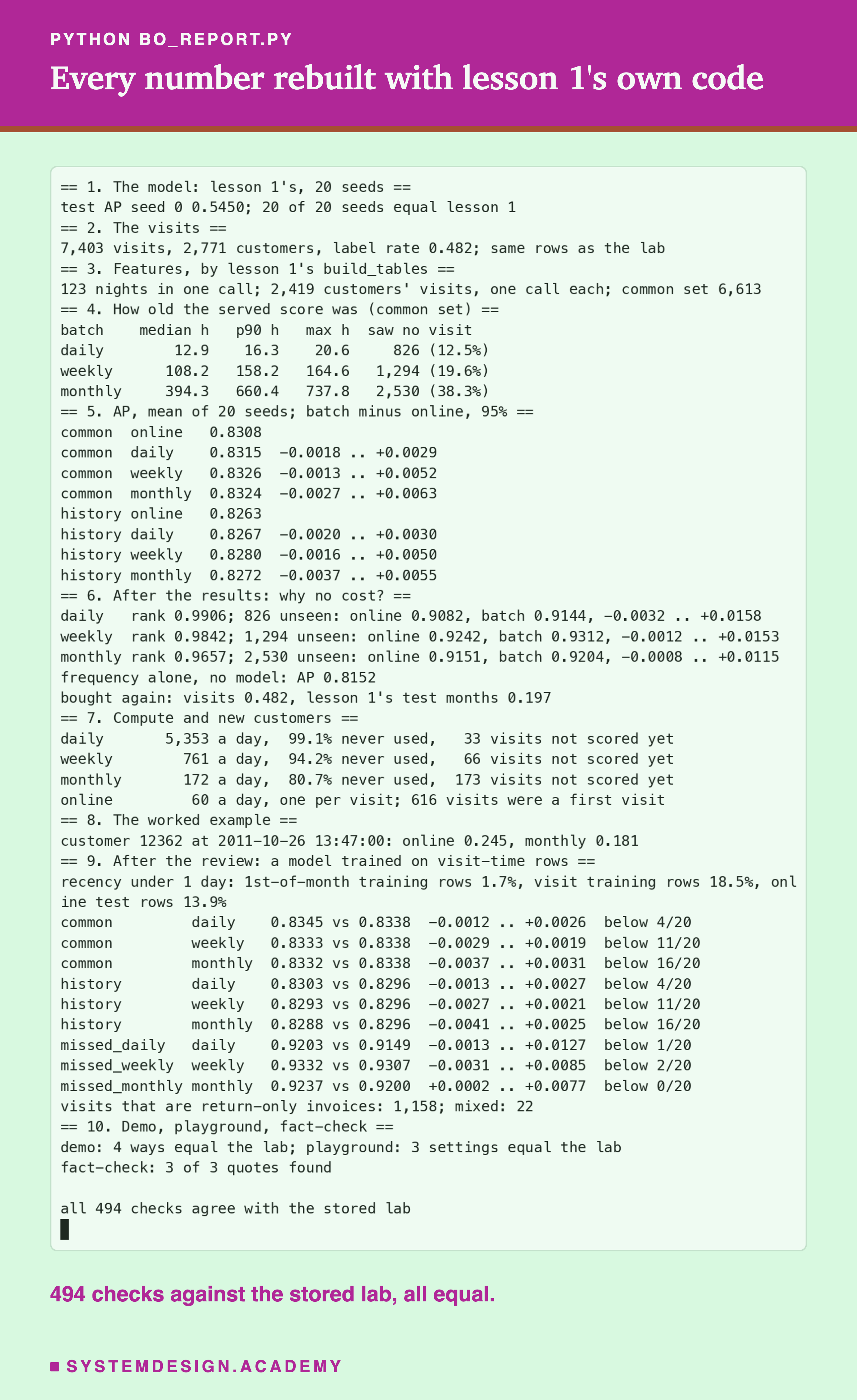
The report does not trust the lab. It never imports the lab's code. It builds every feature with the features chapter's own function, build_tables, which the lab did not use for its main pass. For the batches, it calls that function once for all 123 midnights. For online, it calls it once per customer, with that customer's visit times as the moments to measure at.

It rebuilds the visits and their labels with different pandas code, and trains the 20 models again. It scores every way with scikit-learn's AP, and redoes every bootstrap with an AP function written inside the report. It retrains the visit-time model of the review slide from its own rows too. Then it checks the student demo's stored output, the playground and the fact-check. All 494 checks agreed with the stored lab.

Before any score, here are the requests themselves. Each one is a moment when the shop needed an answer.

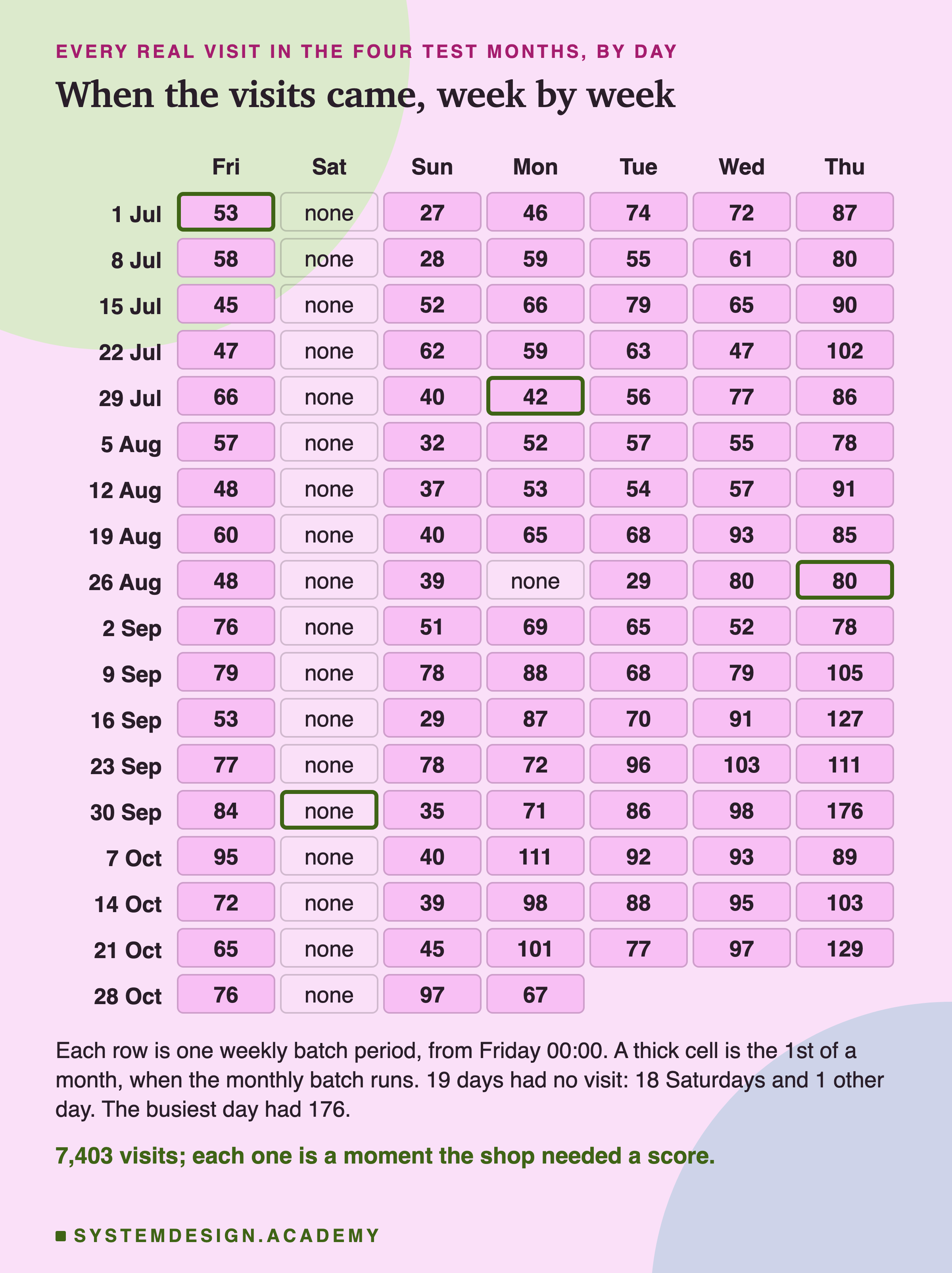
The data has no orders on any Saturday in these months. On the days with orders there were between 27 and 176 visits. The busiest day was Thursday 6 October.

Each row of the calendar is one week of the weekly batch. The job runs at the start of the row, on Friday at midnight. Every visit in that row is served its score. A monthly batch runs on the four thick cells, and its scores serve a whole month.

This picture explains the first cost of online scoring too. The service must be ready on any day at any hour, even if only 27 people come. A batch can run once at night and be switched off. I do not measure money or speed in this lesson, but keep that in mind.

A stored score gets older every hour after the job runs. Here is how old it was at each visit.

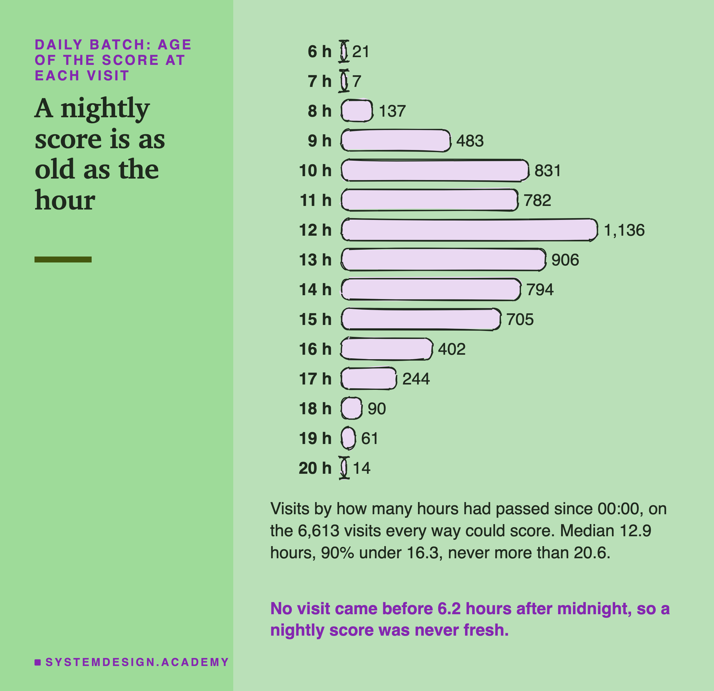
For the daily batch, the age of the score is simply the time of day of the visit. Most orders came between 9 in the morning and 4 in the afternoon. So the typical nightly score was 12.9 hours old when it was used, and it was never fresher than 6.2 hours.

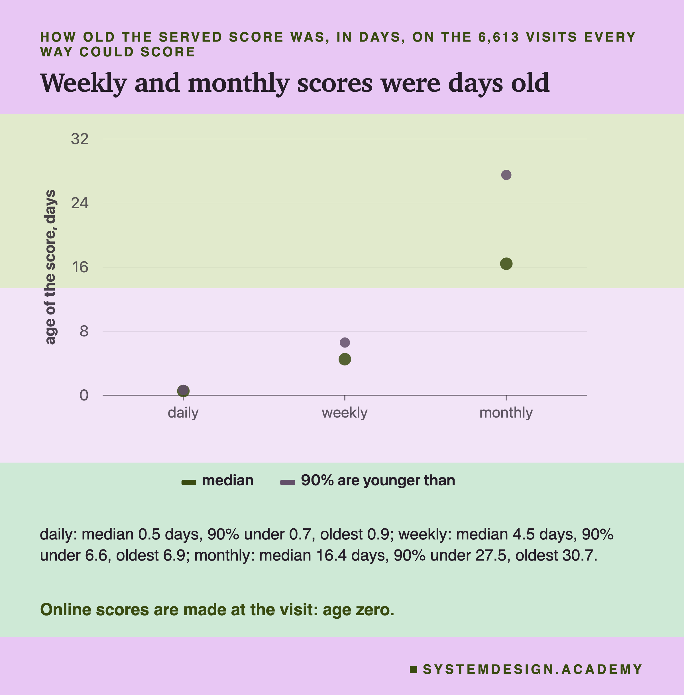
The weekly and monthly scores were much older. Half of the monthly scores were more than 16 days old when a visit used them, and the oldest was 30.7 days. If old scores cost anything, the monthly batch is where I expected to see it.

An old score is only a problem if something happened since it was made. So the lab counted the visits where the same customer had already placed another order between the batch run and this visit.

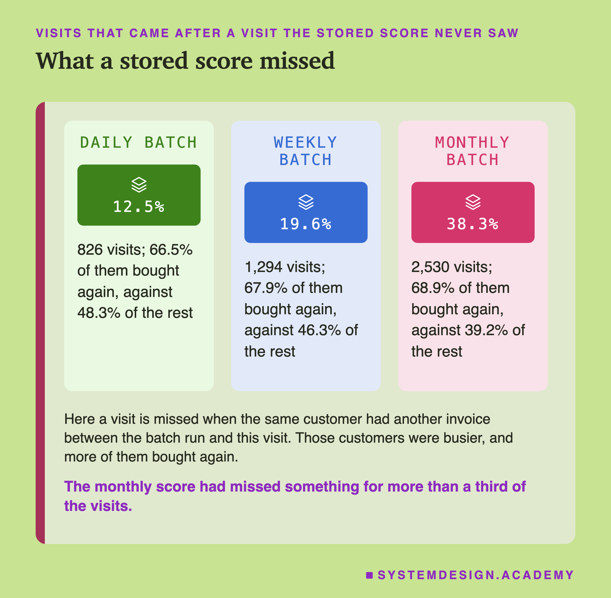
For the daily batch, 826 visits, 12.5%, came from a customer who had another invoice earlier the same day. The stored score did not know about that earlier invoice. For the monthly batch it was 2,530 visits, 38.3%: more than a third of all the visits came after an invoice the monthly score never saw.

And these were not random visits. The customers who came back quickly were busy buyers, and 68.9% of them bought again within 30 days, against 39.2% of the other visits. So the information the stored score missed was exactly about the customers most likely to buy.

This made me confident before the run that the monthly batch would lose AP. The next slide shows that it did not, at least not by an amount this data can see.

Here is the main result. It is AP on the 6,613 visits all four ways could score, as the mean of 20 models.

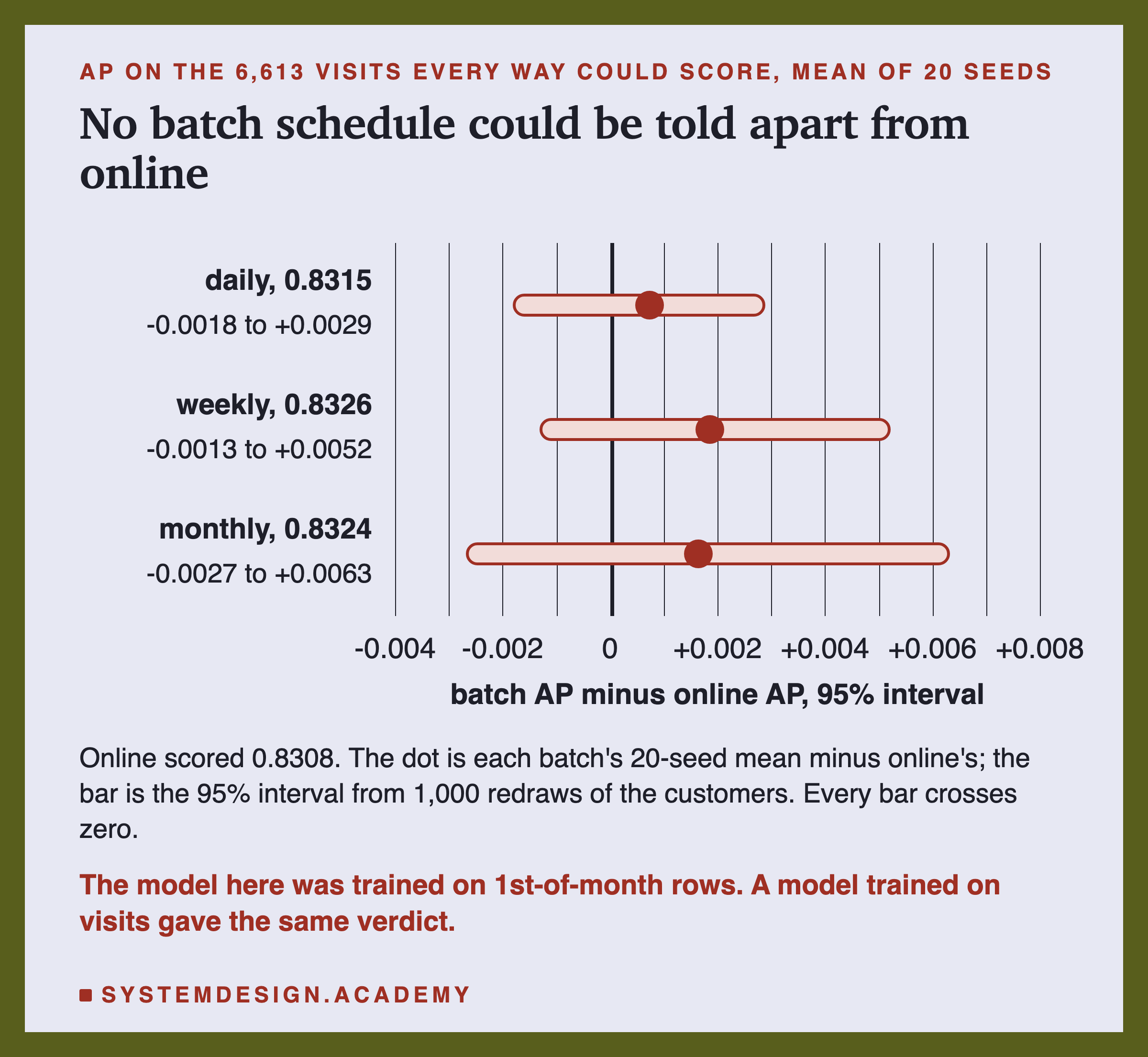
Online scored 0.8308. The daily batch scored 0.8315, the weekly 0.8326 and the monthly 0.8324.

All three batch numbers were a little higher than online, and none of the differences could be told apart from zero. For the monthly batch, the middle 95% of the bootstrap went from -0.0027 to +0.0063. So the data is consistent with the monthly score being a little worse than online, a little better, or the same.

I want to be careful with the words here. This is not "batch is better". The differences are smaller than the luck in the data. And it is not "staleness never matters". It is: on this shop, for this 30-day question, scores up to 30.7 days old cost nothing I could measure.

These numbers come from the features chapter's model, which learned from rows made on the 1st of each month. An independent review pointed out that this tilts the race toward batch, and a later slide measures how much. In short: a second model, trained on visit-time rows, gave the same verdict. With it, no schedule could be told apart from online either.

My guess before the run was that the monthly batch would cost clearly. That guess was wrong, with both models.

The headline uses the mean of 20 models. Here is each model on its own.

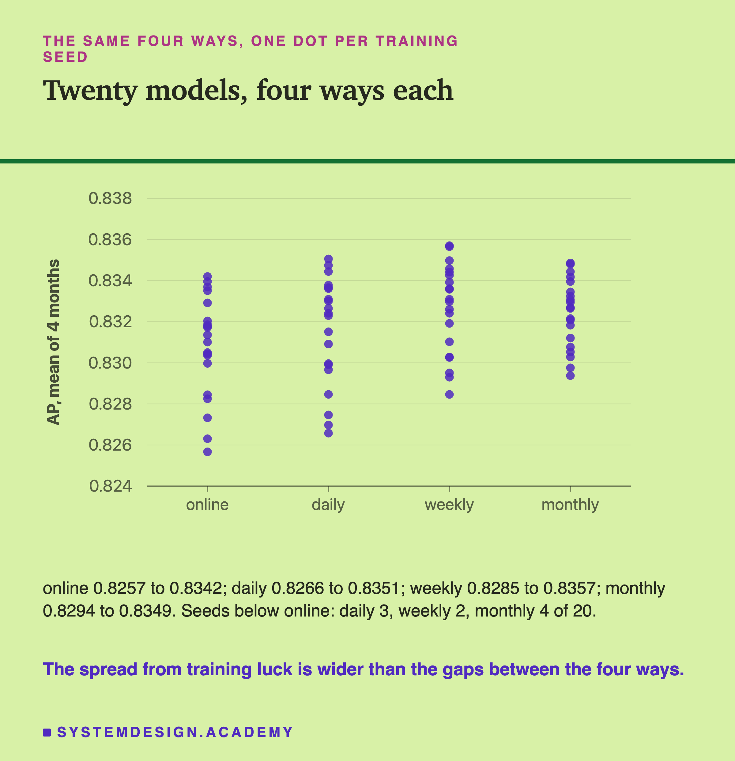
The 20 online models scored from 0.8257 to 0.8342, a spread of about 0.009. The gaps between the four ways were about 0.002 or less. So the choice of seed moved AP more than the choice between batch and online did.

Within each seed, the batch scored below online for only a few of the 20 seeds: 3 for daily, 2 for weekly and 4 for monthly. So the stored scores had a small edge in most seeds, 16 to 18 of 20. The bootstrap on the last slide says that edge is not bigger than customer luck, but a lean in one direction that steady needed a reason.

The review found one. The model learned from rows made at midnight on the 1st of a month. In those training rows, only 1.7% of customers had their last invoice less than a day before, and the median was 61.5 days. In the online test rows, 13.9% did, with a median of 23.0 days. So online asked the model about rows it had rarely seen, while a batch row, also made at midnight, looked more like its training rows. A later slide tests this with a second model.

The common set left out visits from customers a batch had never scored. Here are all 6,787 visits with any history, where each batch serves its fallback score when it has no stored score.

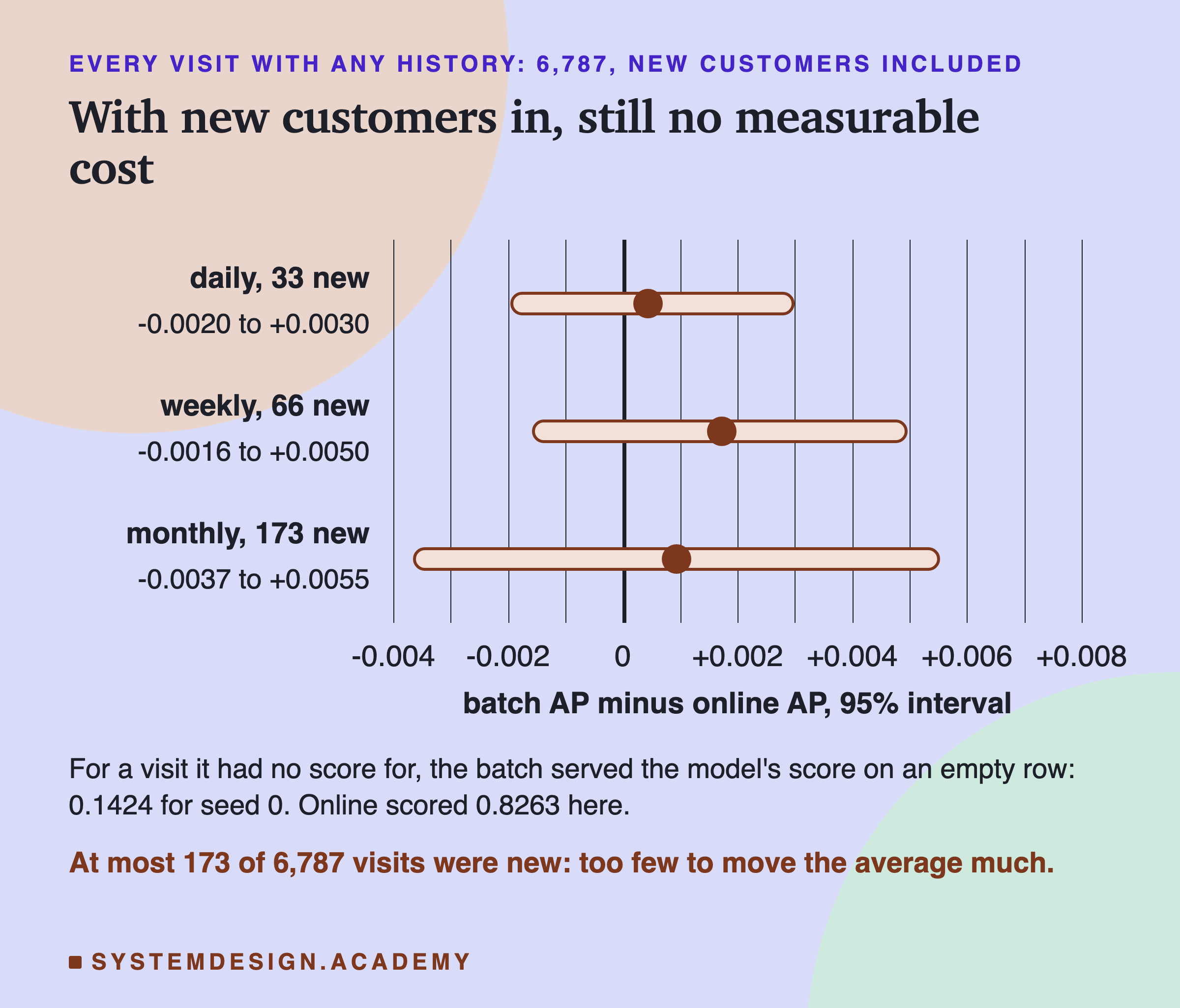
The fallback is the model's score for an empty row, a row with all six numbers missing. For seed 0 it was 0.1424, so a new customer was put fairly low in the ranking. Online, by contrast, could score them from the orders they had already placed.

Even so, every interval still crossed zero. Online scored 0.8263 on this set, and the monthly batch 0.8272. The reason is simple arithmetic: at most 173 of the 6,787 visits were new to the monthly batch, about 2.5%. A worse score on 2.5% of the visits cannot move a mean of all of them very far.

In a business where most visitors are new, this would be very different, and the next slides about new customers come back to it.

Numbers over thousands of visits can hide what happens to one customer. So the lab kept one worked example, chosen by a rule I wrote before the run. The rule: in October, among the visits where the monthly score had missed an earlier order, take the customer with the smallest id.

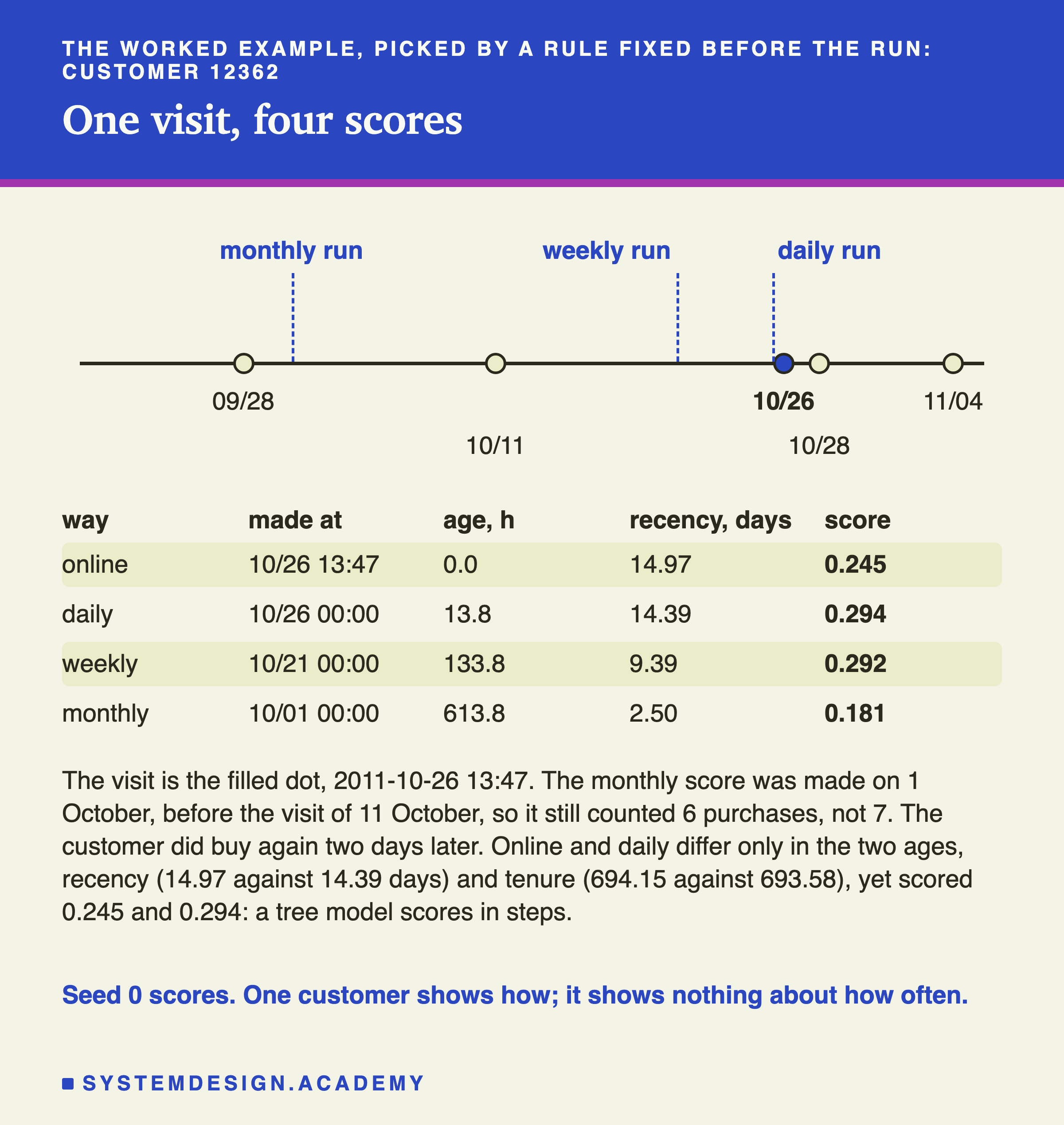
Customer 12362 ordered on 28 September, 11 October and 26 October. On 26 October at 13:47 they came again.

The monthly score was made on 1 October. At that moment the last order was 2.5 days old and they had 6 purchases. It knew nothing about the order of 11 October. So it saw a customer who had just bought, which is a different picture from the online view: last order 15 days ago, 7 purchases.

The four scores went from 0.181 to 0.294. Notice the online and the daily scores. Their inputs differ only in the two ages: recency, 14.97 days against 14.39, and tenure, 694.15 days against 693.58. Yet the scores were 0.245 and 0.294. The model is a set of trees, and a tree answers in steps. A small change that crosses one of its split points can move the score a lot. A change that crosses none moves it not at all.

The customer did buy again, two days later. On this one visit the daily score was "more right" than online. That is one visit, and it says nothing about which way is better in general.

This slide and the next two answer questions I asked after seeing the results. I wrote them into the lab's docstring before that part ran, and the lab labels them as post-results work.

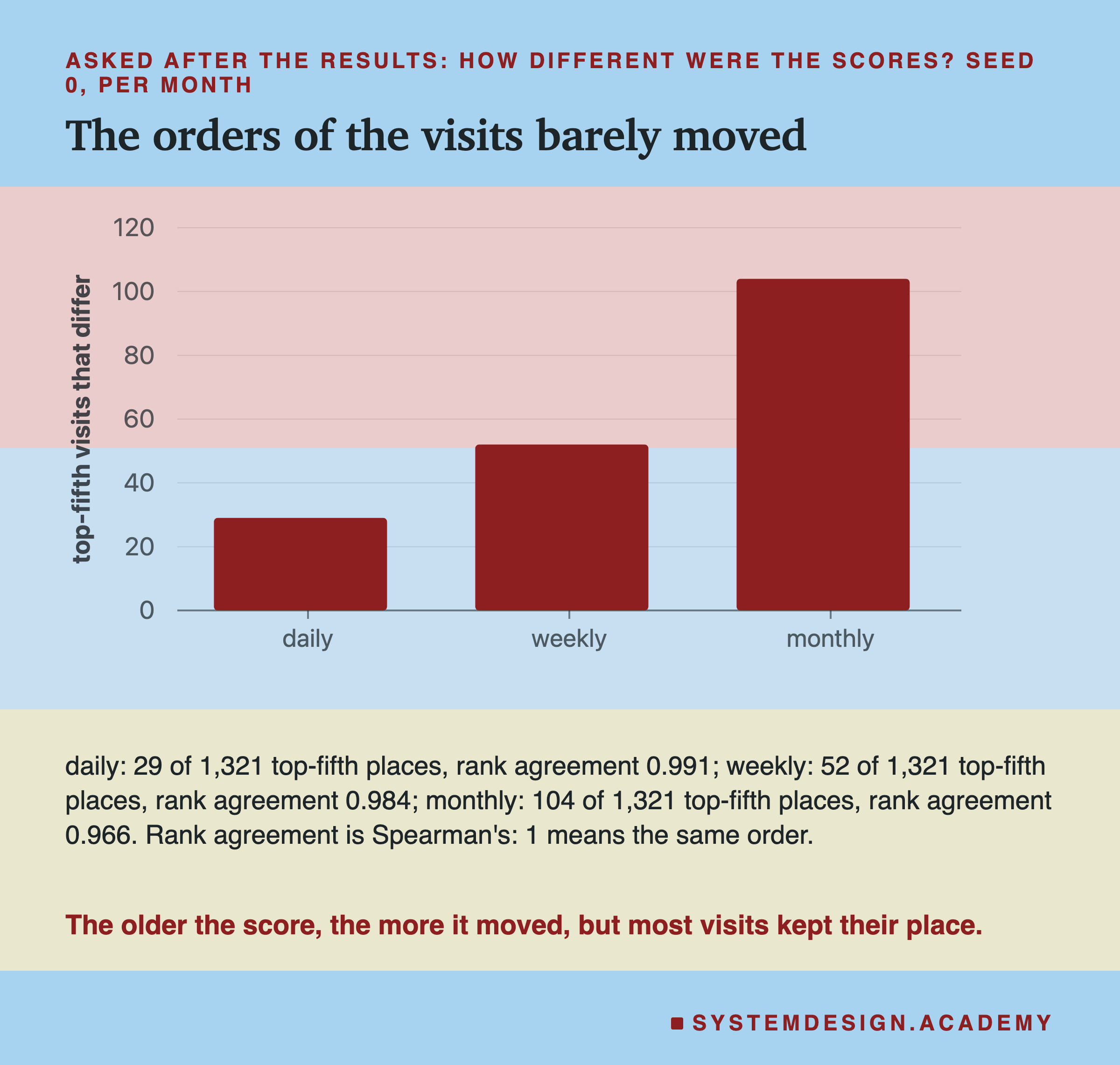
First question: were the stale scores really different from the fresh ones? Rank agreement says how similar two orderings are: 1 means the exact same order. Between online and daily it was 0.991, and between online and monthly 0.966. The top fifth is the 20% of visits each month with the highest scores, the ones a shop would act on first. Of 1,321 top-fifth places, the monthly batch put 104 different visits there than online did. So the old scores did move things, but most visits kept their place.

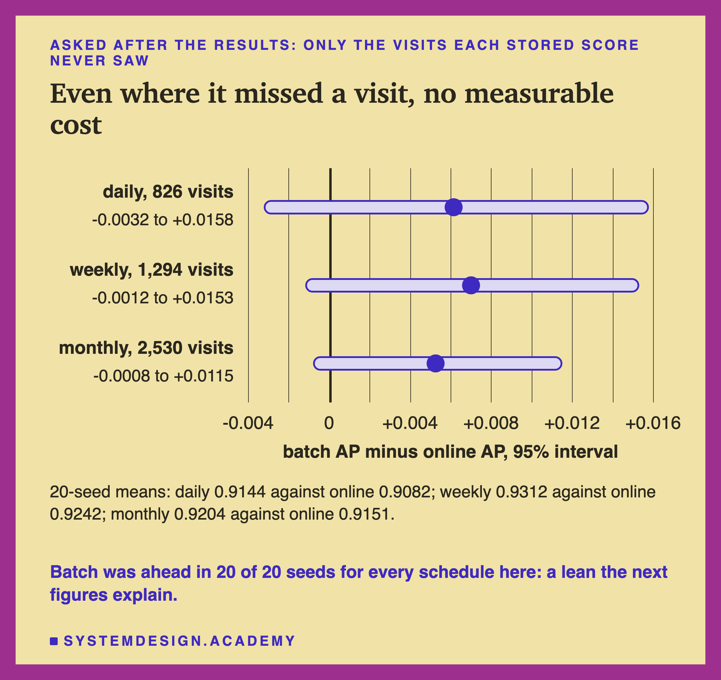
Second question: what about only the visits where the stored score had missed an invoice? If staleness hurt anywhere, it should hurt there. It did not. On the 2,530 such visits, the monthly batch scored 0.9204 and online 0.9151, and the interval, -0.0008 to +0.0115, crossed zero.

But look at the seeds. On these visits, the batch was below online in 0 of 20 seeds, for daily, weekly and monthly alike. Every single model preferred the stale score. This is the lean the review found, at its strongest, and it is why I trained the second model two slides on.

The third post-results question: why is AP so high here, 0.83, when the features chapter's test AP was 0.5450? Not because the model got better. AP depends on how many rows are positive: a random order scores about the share of buyers.

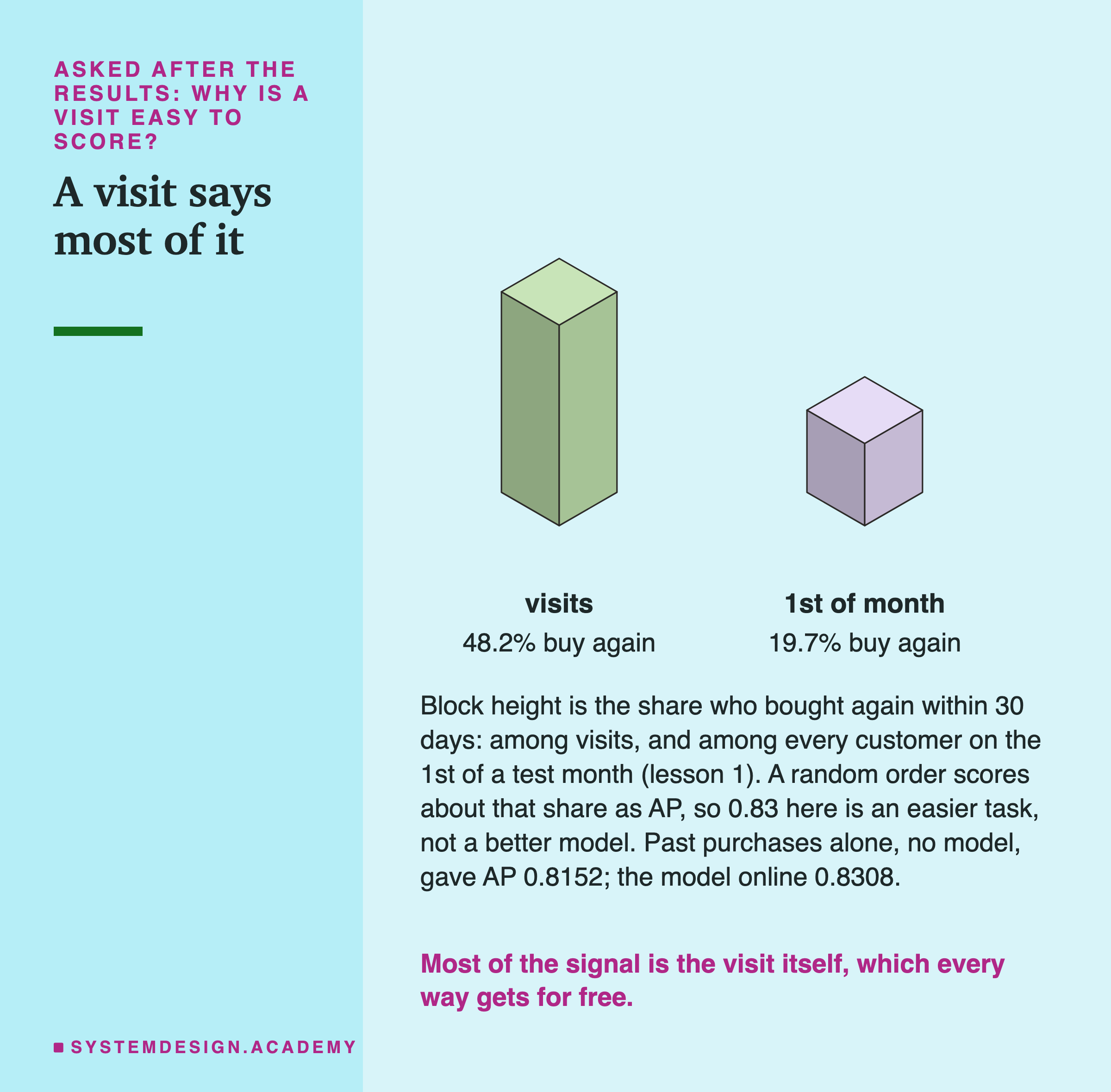
On the 1st of a month, the features chapter scored every customer the shop had ever seen, and only 19.7% of them bought in the next 30 days. Here, every row is a customer who is ordering right now. Among them, 48.2% bought again within 30 days. A customer who is placing an order is, almost by definition, an active customer.

Then I tried a rule with no model at all: rank the visits by how many orders the customer had placed before. That alone gave AP 0.8152. The model online gave 0.8308. So most of the ranking comes from two facts every way already has: this person is visiting, and how often they bought before. The number of past orders changes slowly, so a month-old copy of it is nearly as good as a fresh one.

So 0.83 here and 0.5450 there measure different tasks. A random order would score about 0.48 here and about 0.20 there. The visit task is easier, and the model is the same.

This is my best explanation of why staleness cost little here. It fits the numbers, but I have not proved it.

This slide answers the independent review. Its design was written into the lab's docstring before it ran, and the lab labels it as post-review work.

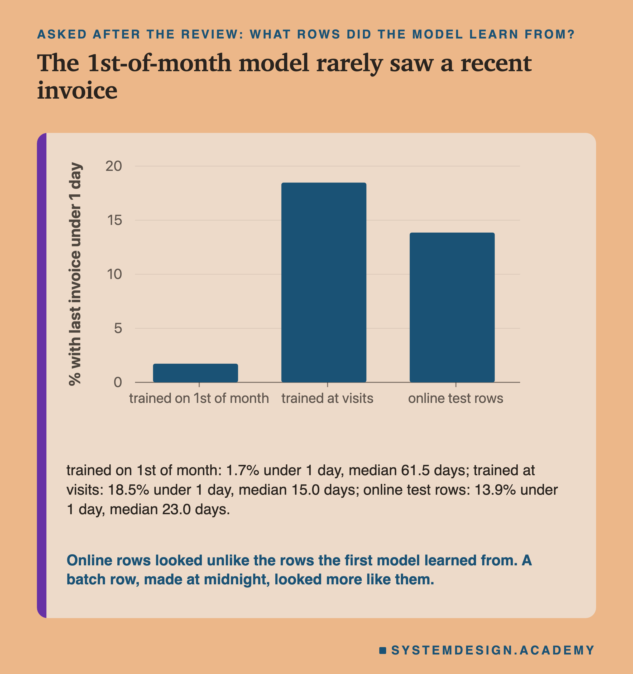
The first model learned from 44,521 rows made at midnight on the 1st of each month. Only 1.7% of them had a last invoice under a day old. So I built a second training set the same way as the test visits. It holds every invoice in the training months, March 2010 to February 2011, with the six numbers worked out from everything strictly before it. Its label is "buys again within 30 days after it". That gave 19,404 rows.

In them, 18.5% had a last invoice under a day old, close to the online test rows' 13.9%. I trained 20 models on these rows and served the same test visits the same four ways.

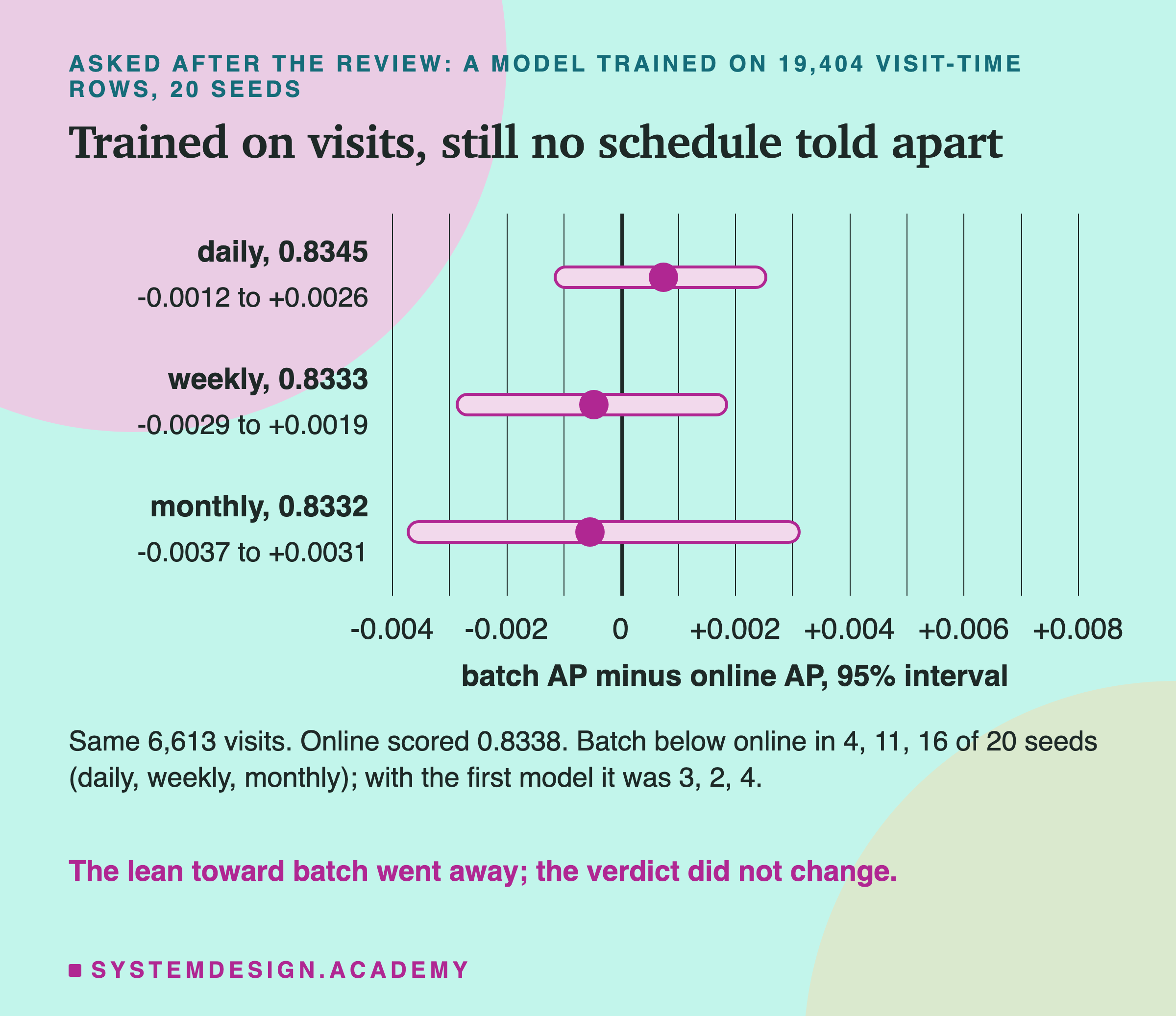
The lean went away. With the visit-trained model, the monthly batch was below online in 16 of 20 seeds, where the first model had it below in only 4. Weekly was below in 11. So the review was right: part of the old edge for stored scores came from the training rows.

The verdict did not change. Every interval still crossed zero: monthly -0.0037 to +0.0031, weekly -0.0029 to +0.0019, daily -0.0012 to +0.0026. With either model, no schedule could be told apart from online on this shop.

I also checked the visits each stored score missed. With the visit-trained model, the daily and weekly intervals crossed zero. The monthly one did not: the monthly score was ahead, +0.0002 to +0.0077, in all 20 seeds. That is one interval out of nine I computed with this model, and it barely clears zero. I do not know why, and I do not read it as "stale is better". With nine tries, one this close to zero can come from luck.

Staleness was not the cost. Waste was. A batch scores every customer the shop has ever seen, every time it runs. Online scores only the customers who show up.

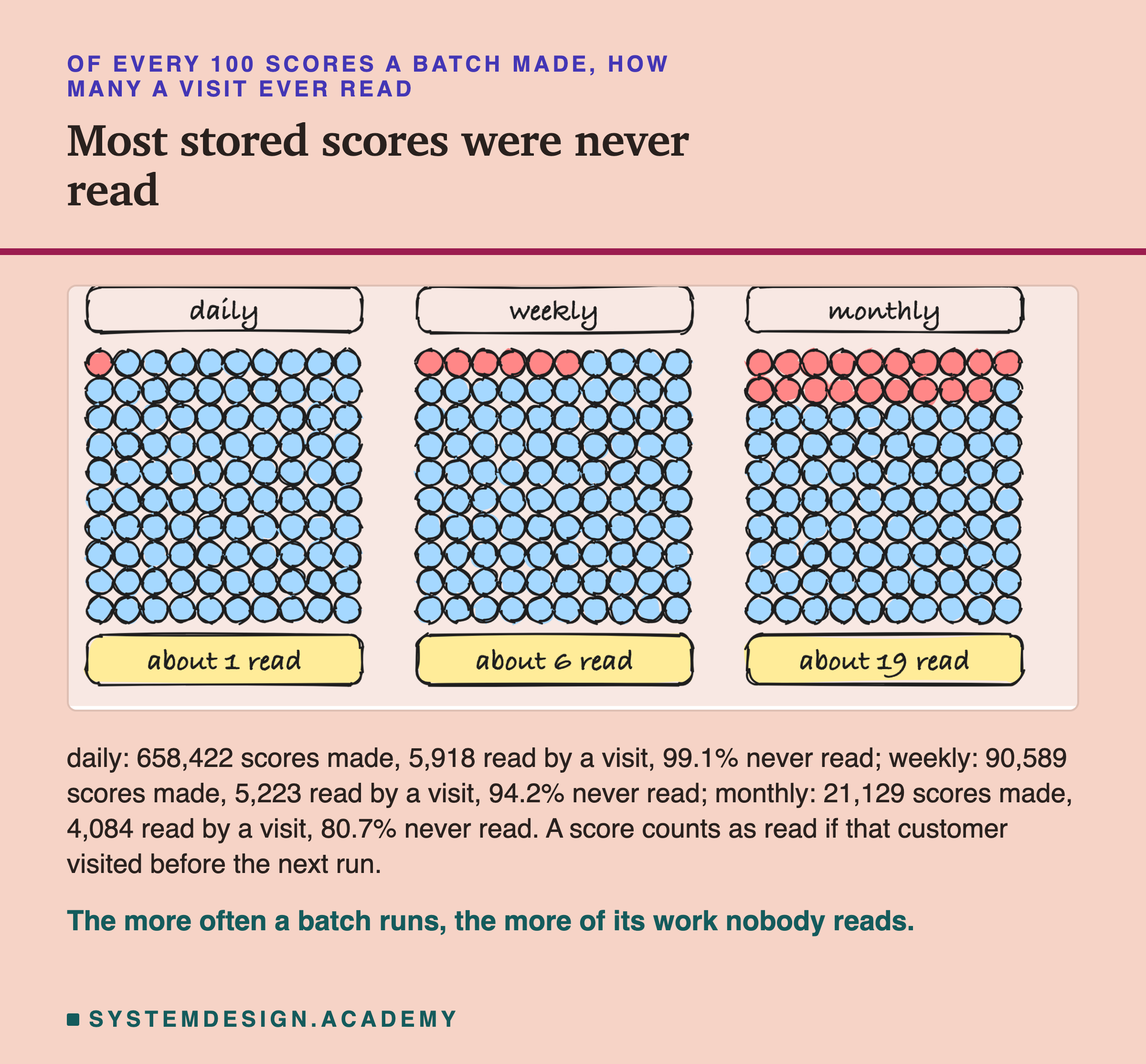
I counted a stored score as read if that customer made at least one visit before the next run replaced it. The daily batch made 658,422 scores over 123 nights, and only 5,918 of them were ever read: 99.1% were never used. The monthly batch wasted less, 80.7%, because a month is long enough for more customers to come back.

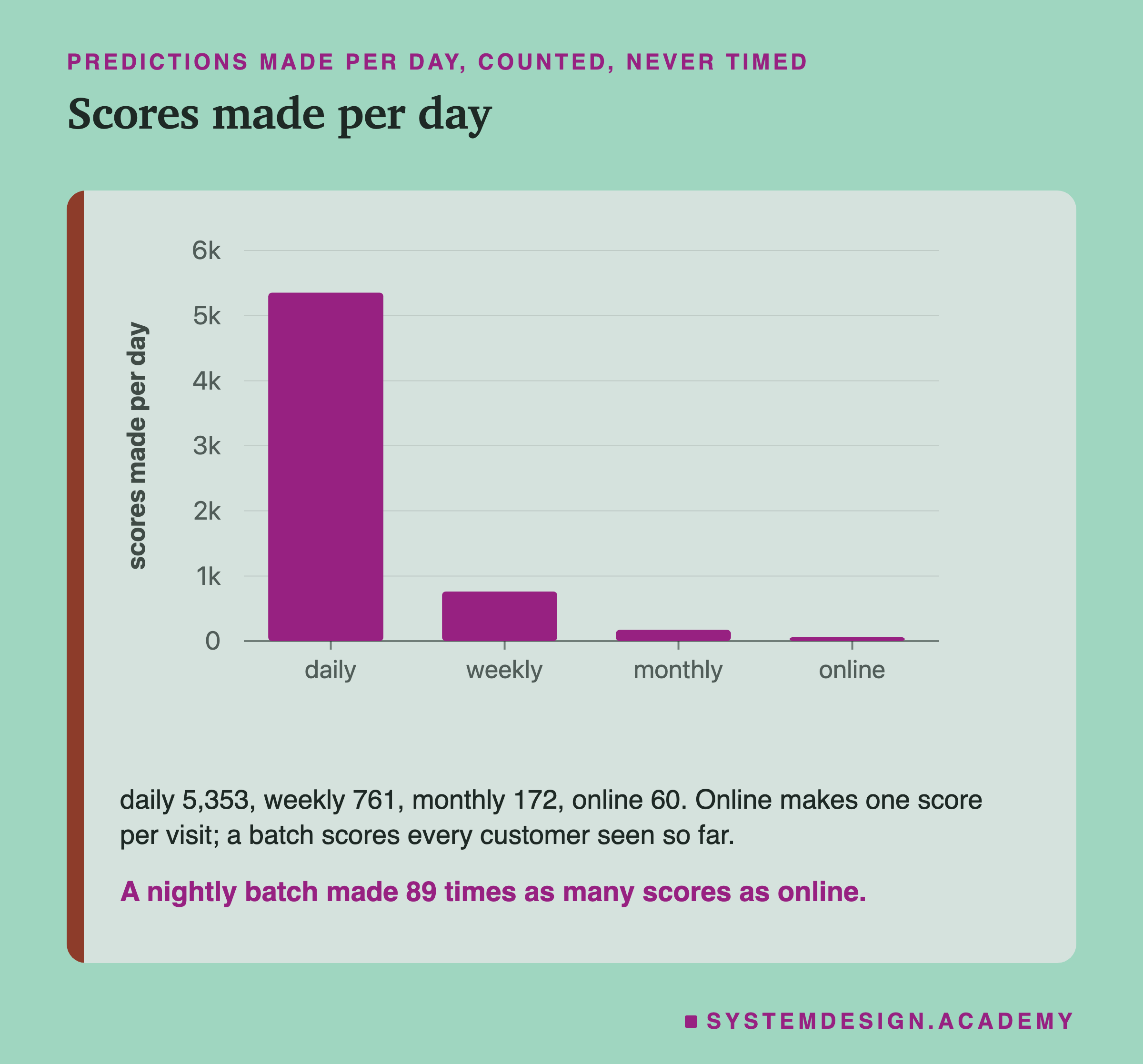
Per day, the nightly batch made 5,353 scores and online made 60, one per visit. These are counts, not times. I did not measure how long a score takes on this laptop. The laptop was busy with other work, and the chapter's rule is that timings come only from a quiet machine. For this small model a few thousand scores a night may cost very little. For a large model, or millions of customers, 99% waste is real money.

The other cost of a batch is the customers it has not met yet.

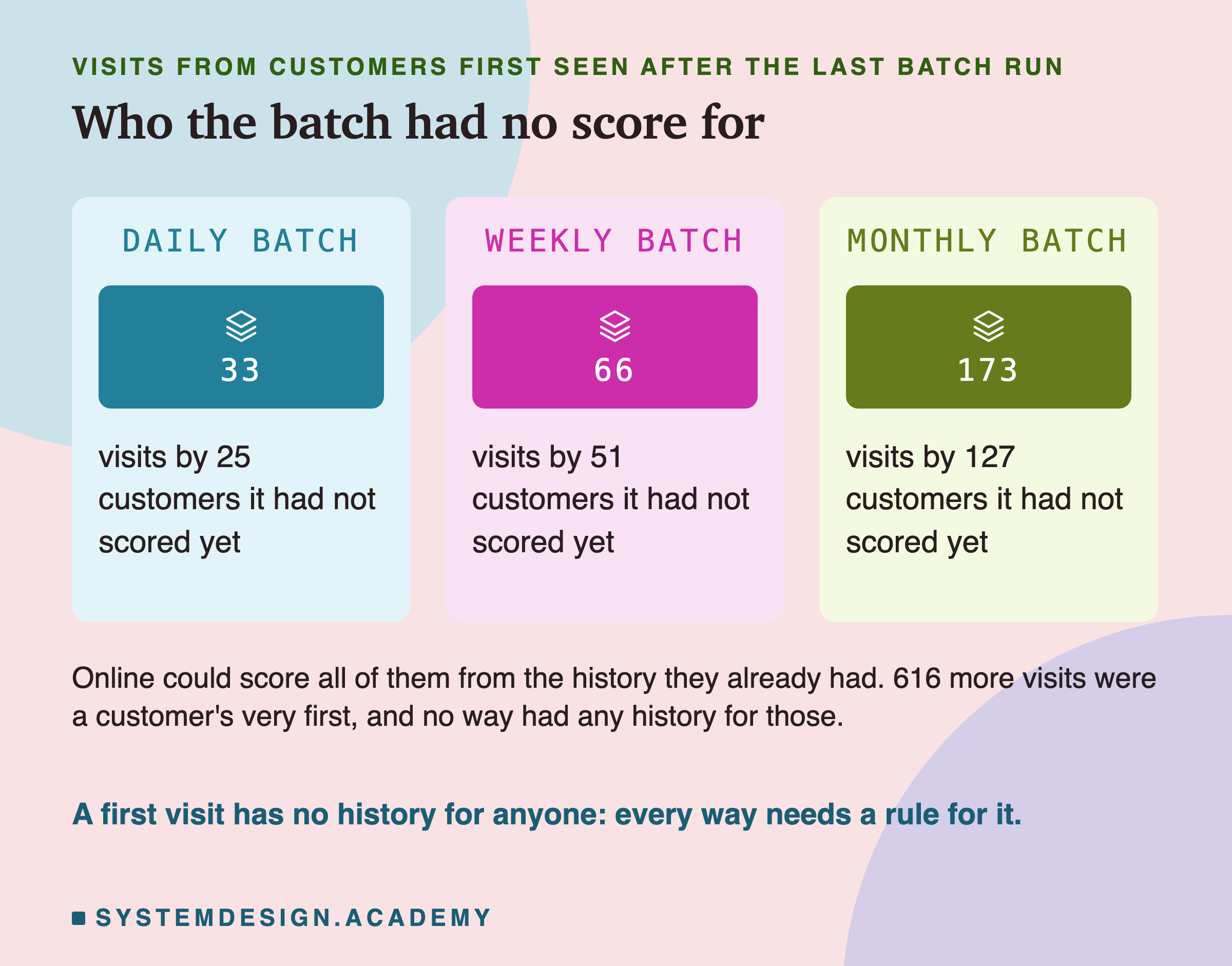
A new customer here is someone whose first invoice came after the last batch run, and who then came back before the next one. The daily batch missed 33 such visits, by 25 customers: people with two invoices on their first day. The monthly batch missed 173 visits, by 127 customers: anyone whose first invoice came earlier in the month. Online scored all of them from the invoices they already had.

There is a bigger group that no way could help: 616 visits were a customer's very first invoice. Nobody had any history for them, online included. A shop that wants a score at a first visit needs a rule for it, such as the fallback, whichever way it serves.

In this shop, new customers were a small share of the visits. In a shop that grows fast, or a website where most visitors are new, the batch would have no score for a large share of requests. Then the choice is no longer close.

The lab made online scoring look easy, and I should be honest about why. In the lab, online scoring had a perfect record of every past order, ready at the exact second of each visit. A real shop does not get that for free.

The numbers must be ready at request time. To score a visit at 13:47, the service needs the customer's six numbers as they are at 13:47. Someone has to keep a store of those numbers up to date as orders arrive. In the features chapter, late events and watermarks showed that events can arrive late, so the "fresh" numbers may not be quite fresh.

Two copies of the feature code must agree. A batch job usually computes features one way, over a whole table. An online service computes them another way, one customer at a time. In online and offline consistency, two correct versions of the same features still disagreed in the last digits on 17,670 of 26,851 test rows. Here, the lab avoided that by using one pass for both, and checked it against the chapter's own function.

The service must be up all day. A batch job can fail at 02:00 and run again at 03:00, and nobody notices. An online service that fails at 13:47 fails a real visit.

None of these costs showed up in my AP numbers, because the lab did not have to pay them. The rest of this chapter measures some of them on a quiet machine. It asks where the time in one request goes, what the slowest requests look like, and what a request should get when a part of the system is slow.

This result should not surprise you if you read the two earlier lessons together. They measured the two ends, and this lesson sits between them.

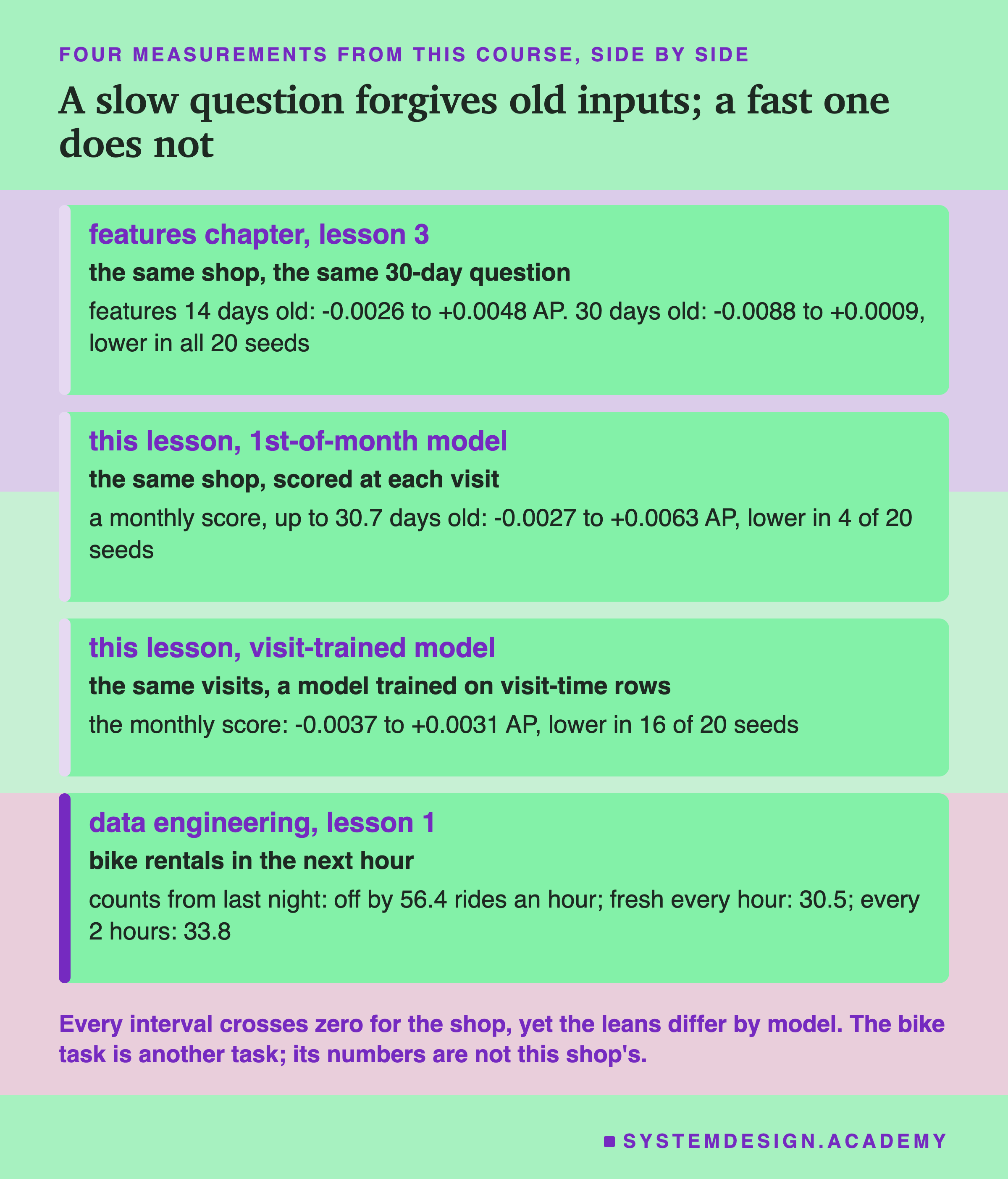
Feature freshness served this shop's model features up to 14 days old and could not measure any cost. At 30 days it was closer: all 20 seeds scored below fresh, on average by 0.0037, though the interval, -0.0088 to +0.0009, still crossed zero. That lean is the opposite of this lesson's first model, which put the monthly score ahead in 16 of 20 seeds.

The review explains the difference. In the freshness lesson, the model was trained and tested on 1st-of-month rows, so stale and fresh rows were both judged by a model that knew their shape. Here, the first model had never learned what a visit-time row looks like. Trained on visit rows, the monthly score fell below online in 16 of 20 seeds, the same lean as the freshness lesson, and again too small to separate from luck.

Batch vs streaming data asked a fast question: how many bikes will be rented in the next hour? There, the count from last night was off by 56.4 rides an hour on average, and the count made fresh every hour by 30.5. Freshness almost halved the error.

So the honest answer to "batch or online?" depends on how fast your answer changes. For a fraud check on a card payment, a news feed, or anything that changes within hours, an old score can be badly wrong. I have not measured those tasks here, so I give no numbers for them.

I wrote four guesses into the lab before it ran. Here they are against the results.

1. "daily costs nothing the bootstrap can tell from zero on the common set; weekly costs little; monthly costs clearly (its interval below zero)." Right for daily. Wrong for weekly and monthly: neither could be told apart from online. With the first model both were a little ahead on average; with the visit-trained model both were a little behind.

2. "most batch predictions are never used: more than 90% for daily." Right: 99.1%.

3. "online makes far fewer predictions per day than daily batch." Right: 60 against 5,353.

4. "new customers: few under daily (only a second visit on the first day), many under monthly." Right in direction: 33 visits against 173. But "many" was too strong. Even 173 was only about 2.5% of the visits with history.

The one I got most wrong is the one I was most sure of. I had looked at the share of visits the monthly score missed, 38.3%, and decided it must cost AP. It did not, because the missed orders changed the ranking less than I thought, as the post-results slides show. This is why the lab measures before the lesson claims.

The full lab trains 20 models and redraws the customers thousands of times. I wrote a smaller demo that does the heart of it with one model.

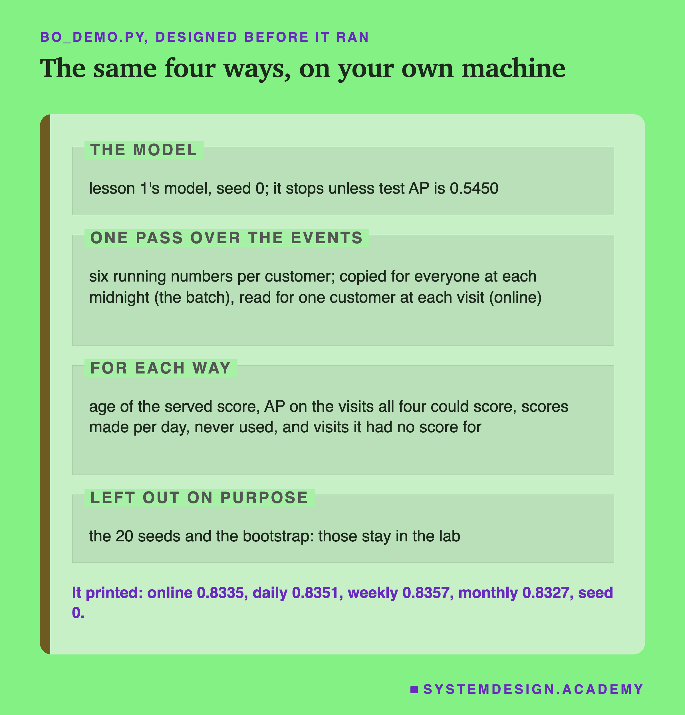
I wrote the demo's design into its docstring after the lab had run and before the demo first ran. It trains the model with seed 0 and makes one pass over the shop's orders in time order. For each customer it keeps six running numbers. At every midnight it copies them for every customer seen so far: that copy is the batch. At every visit it reads that one customer's numbers as they are right then: that is online. Weekly and monthly batches reuse the midnight copies, because they also run at midnight.

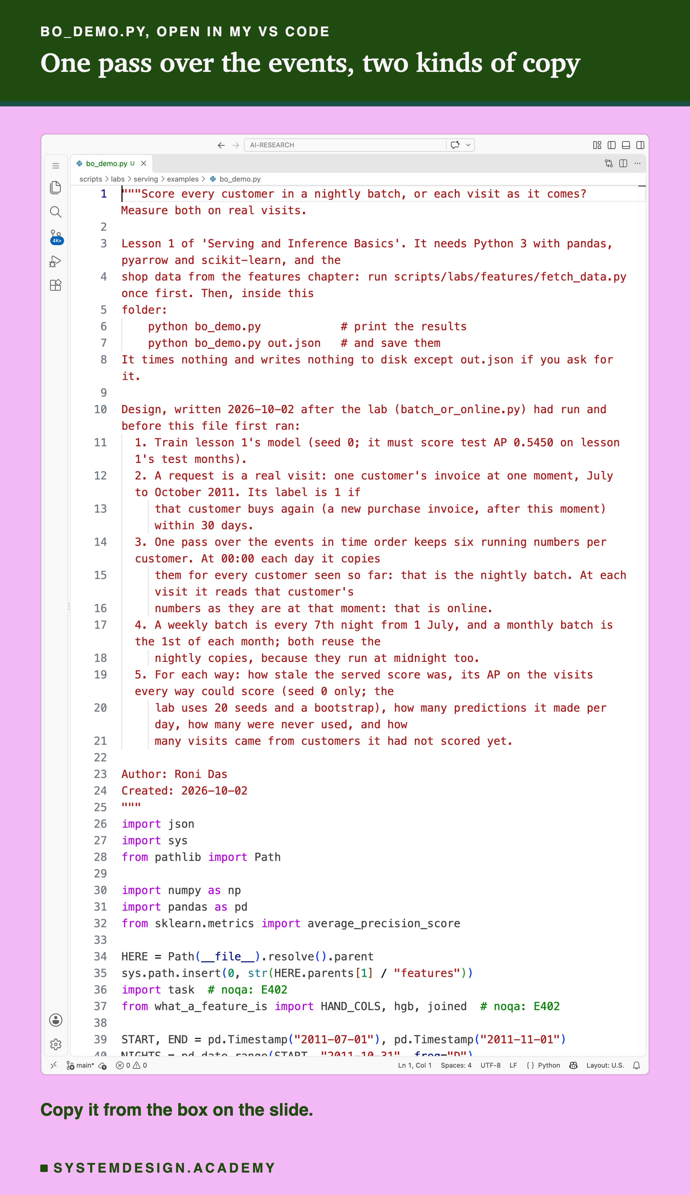
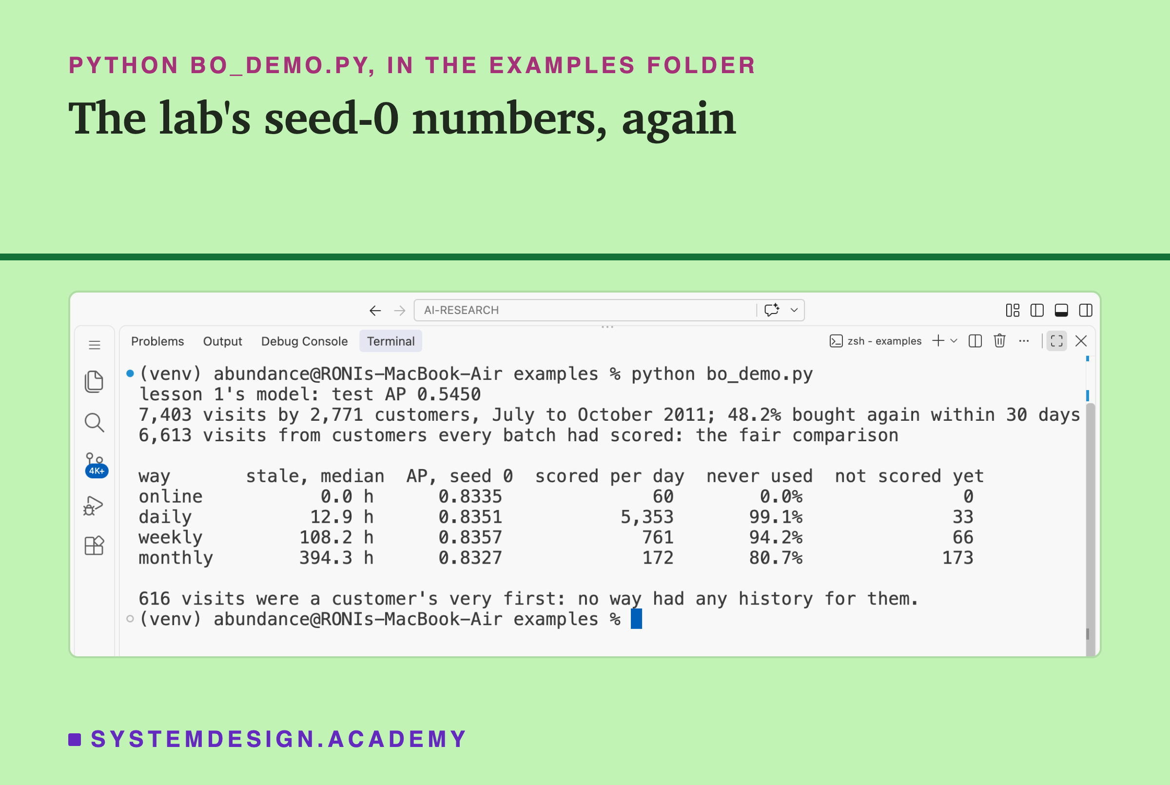
Before you run this lab. You need Python 3 with pandas, pyarrow and scikit-learn: pip install pandas pyarrow scikit-learn openpyxl. First run python fetch_data.py from the scripts/labs/features folder. It downloads the shop data once, about 46 MB, and writes one cleaned file. Then, inside the examples folder of scripts/labs/serving, run python bo_demo.py. It needs no GPU. I ran it with scikit-learn 1.9.1 and Python 3.13 on a Mac. Another version of scikit-learn may give slightly different decimals. The pattern should hold: no batch far from online, and most batch scores never read.

This box holds the real results from the lab. It needs nothing but Python, so it runs in your browser. It has no model inside; it looks up what the lab measured.

Press Run. Then change SCHEDULE to "daily" or "weekly" and run it again. At the bottom, the box also does some plain arithmetic with numbers you choose. Put in your own number of customers, visitors per day and days between batch runs. It shows at least how many batch scores would never be read. That part is arithmetic, not a measurement.

The report script writes this box from the lab's stored results, runs it for all three schedules, and checks what it prints against the lab. For the arithmetic at the bottom, "at least" is honest: if the same customers visit on several days, even fewer scores are read.

The lab is one file, scripts/labs/serving/batch_or_online.py. Here is what each part does.

build_requests finds every distinct customer and order time between 1 July and 31 October 2011, and works out each label: does the same customer buy again after this moment and within 30 days?

snapshots is the one pass over the events in time order. It keeps six running numbers per customer and copies them at every batch run and at every visit. kahan_add adds money up exactly the way pandas adds a group, so the numbers match the features chapter to the last digit; features_from_state turns the running numbers into the six features with the same date arithmetic.

main trains the 20 models and checks each against the stored test AP, checks the features at 124 midnights and 300 random visits against the features chapter's own function, then serves every visit four ways. served_run finds the last batch run before each visit. ap_months works out AP per month, and bootstrap redraws customers within each month 1,000 times and keeps the 20-seed mean difference each time.

visit holds the post-review arm: it builds visit-time training rows from March 2010 to February 2011, trains 20 models on them, and serves the same test visits four ways again. holds the three questions asked after the results: rank agreement, the missed visits only, and the no-model rule. downloads each source at a fixed version and searches for every quote. only counts visits per day for the calendar figure; it was also added after the run.

Here is the order of questions I would ask before choosing, using what this lab and the two earlier ones measured.

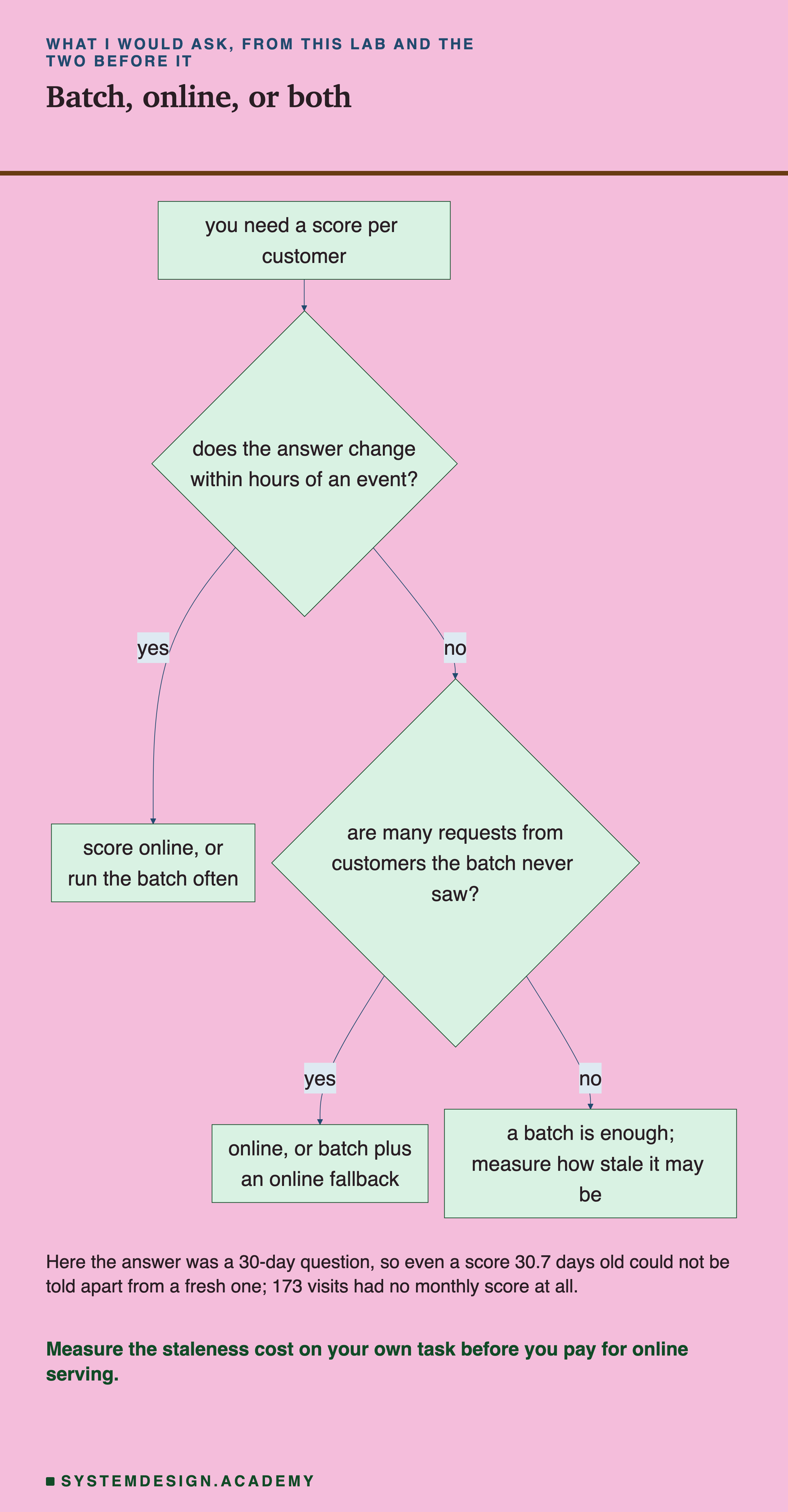
The chart asks the slow-or-fast question first, because on this shop it decided everything: a 30-day answer made even old scores good enough. Here are the same steps in words, each with the number behind it.

1. Ask how fast the answer changes. If one event can change the right answer within hours, a stored score goes bad fast. Bike rentals in the next hour were like that. This shop's 30-day question was not.

2. Count who arrives without a stored score. Here it was at most 173 of 6,787 visits for the monthly batch. If it is a large share for you, a batch alone will serve many guesses.

3. Replay real requests against stored scores of each age. That is what this lab did. It is cheap, it needs only your logs and your model, and it tells you the cost of staleness on your task instead of a guess.

4. Count the waste. If 99% of batch scores are never read and each score is expensive, online may save money even when staleness costs nothing.

5. Remember the mix. Many real systems do both: a batch fills a store, as Feast's materialize_incremental does, and an online path covers the new customers.

Use a batch when the answer changes slowly. Here, on a 30-day question, scores up to 30.7 days old could not be told apart from fresh ones. A batch is simple, can run when the machines are quiet, and does not need a service that is ready all day.

Do not use a batch when the answer changes within hours. The bike lesson measured that a count from last night nearly doubled the error against a fresh one. A stored score would carry the same problem.

Use online when many requests come from customers the batch has never seen. A batch can only serve a fallback for them. Here that was a small share; on a fast-growing site it may be most of the traffic.

Use online when most stored scores would never be read and each score is costly. The nightly batch here wasted 99.1% of its scores. For a small model that may not matter; for a large one it does.

Do not choose online just because it sounds more modern. It needs a service that works every hour, features that can be computed fast at request time, and the same feature code in training and serving. On this shop, with either model, all of that would buy no measurable gain in ranking.

Do not trust one seed or one customer. Seed 0 alone put the monthly batch below online; 20 seeds put it slightly above; the bootstrap says neither is a real difference.

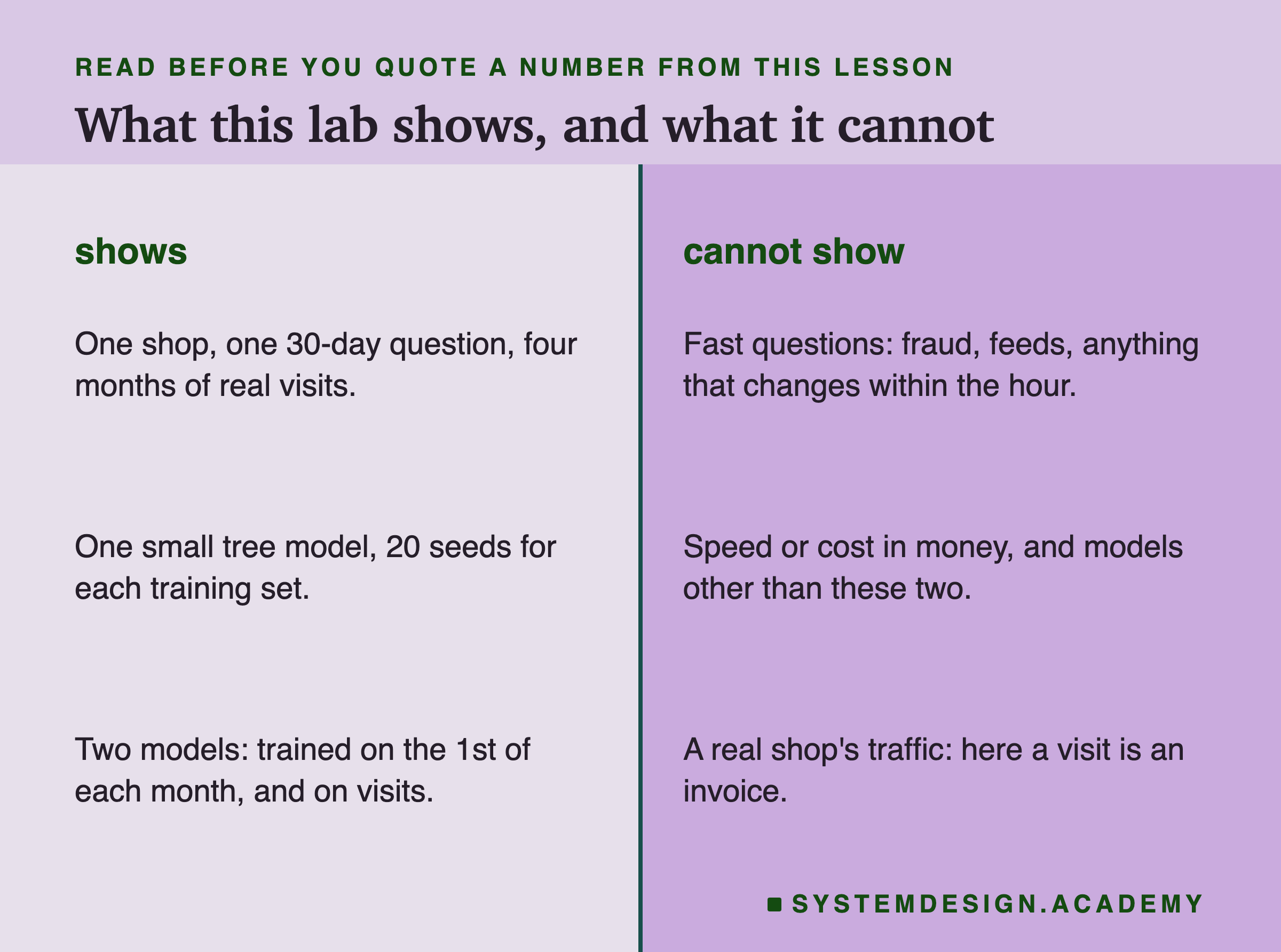
One shop, one slow question. Everything here is one UK gift wholesaler and one 30-day question. I make no claim about fast questions, and I give no numbers for them.

A visit is an invoice. Real websites have visits that end without an invoice. This data only has invoices, orders and returns, so "a request" here is an invoice; about 1 in 6 was a return. A shop that scores every page view would see many more requests, and many more customers with no history.

Two models, not every model. The first model was trained on 1st-of-month rows, which leaned the race toward batch. The second, trained on visit-time rows, removed that lean. Other models, or more features that change by the hour, could behave differently.

The bootstrap is a little optimistic. It redraws customers within each month, so a customer's visits in different months are treated as separate. They are not, so the true intervals may be slightly wider than shown.

No timings and no money. Nothing was timed on this laptop, by the chapter's rule. The next lessons measure time on a quiet machine.

Labelled additions. The three post-results questions, the visits-per-day count and the fact-check mode were added after the main run. The visit-trained model was added after an independent review. The lab labels each one.

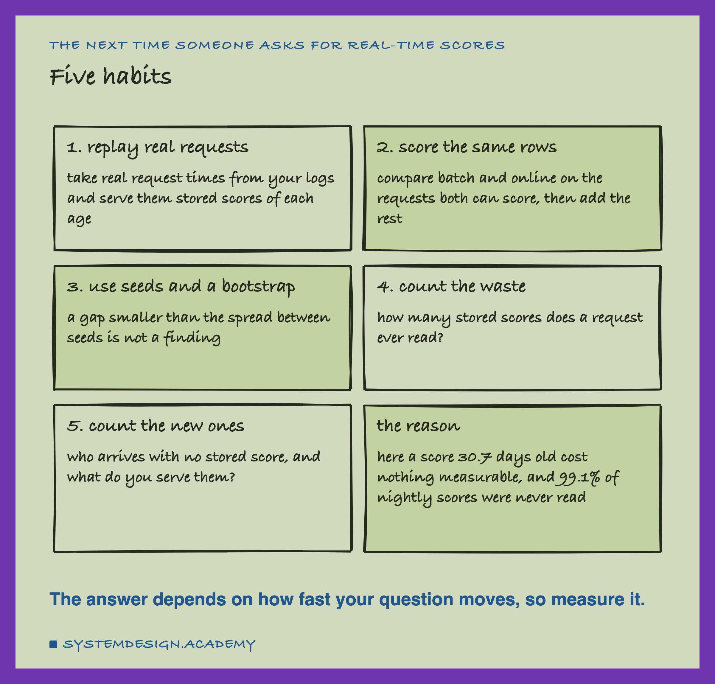
If someone on your team asks for real-time scores on Monday, do not argue from feelings. Take a week of real request times from your logs. For each request, work out what a nightly, weekly or monthly batch would have served, and what an online score would have been. Compare them on the same requests, with several seeds and a bootstrap. Count how many stored scores were ever read, and how many requests had no stored score.

That replay takes your existing model and your existing logs, and it answers the question for your task instead of for mine.

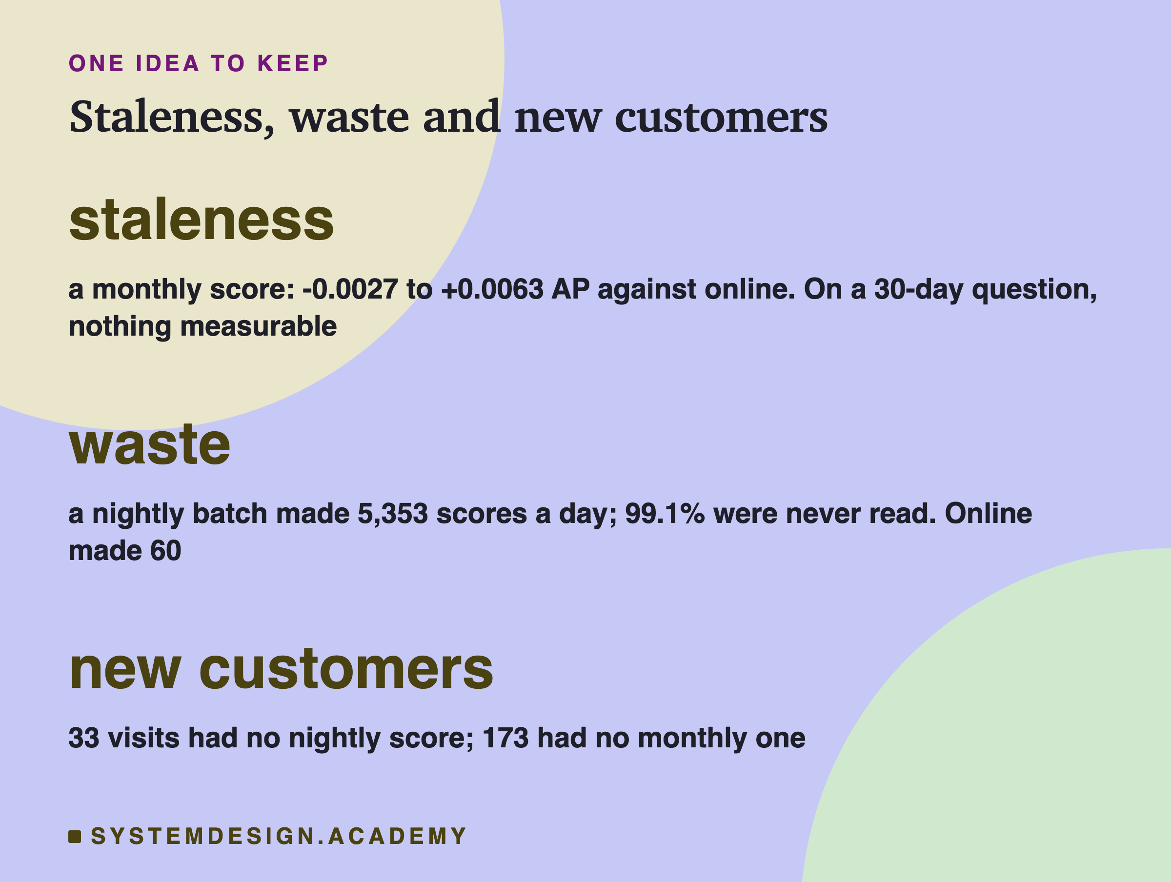
The one idea to keep: "batch or online" is three questions, not one. How much does an old score cost? Here, on a slow question, nothing I could measure. How much batch work is wasted? Here, 99.1% of the nightly scores. Who arrives with no score? Here, a small share. Measure all three on your own task before you choose.