Imagine a bakery with twenty shops that has sold the same bread for years. The head baker has a new recipe that is cheaper to make. She thinks it tastes just as good, but she is not sure, and a bad loaf in every shop at once would cost her customers. So she has two careful ways to try it.

The first way: sell the new loaf in one shop out of twenty and keep the old loaf everywhere else. Then count the complaints. If the one shop gets more complaints than the other nineteen, the new loaf is probably worse. The trouble is that the shops are different. One shop is near a school and gets fussy children; another is near an office and gets people in a hurry. A few extra complaints in one shop may say more about its customers than about the bread.

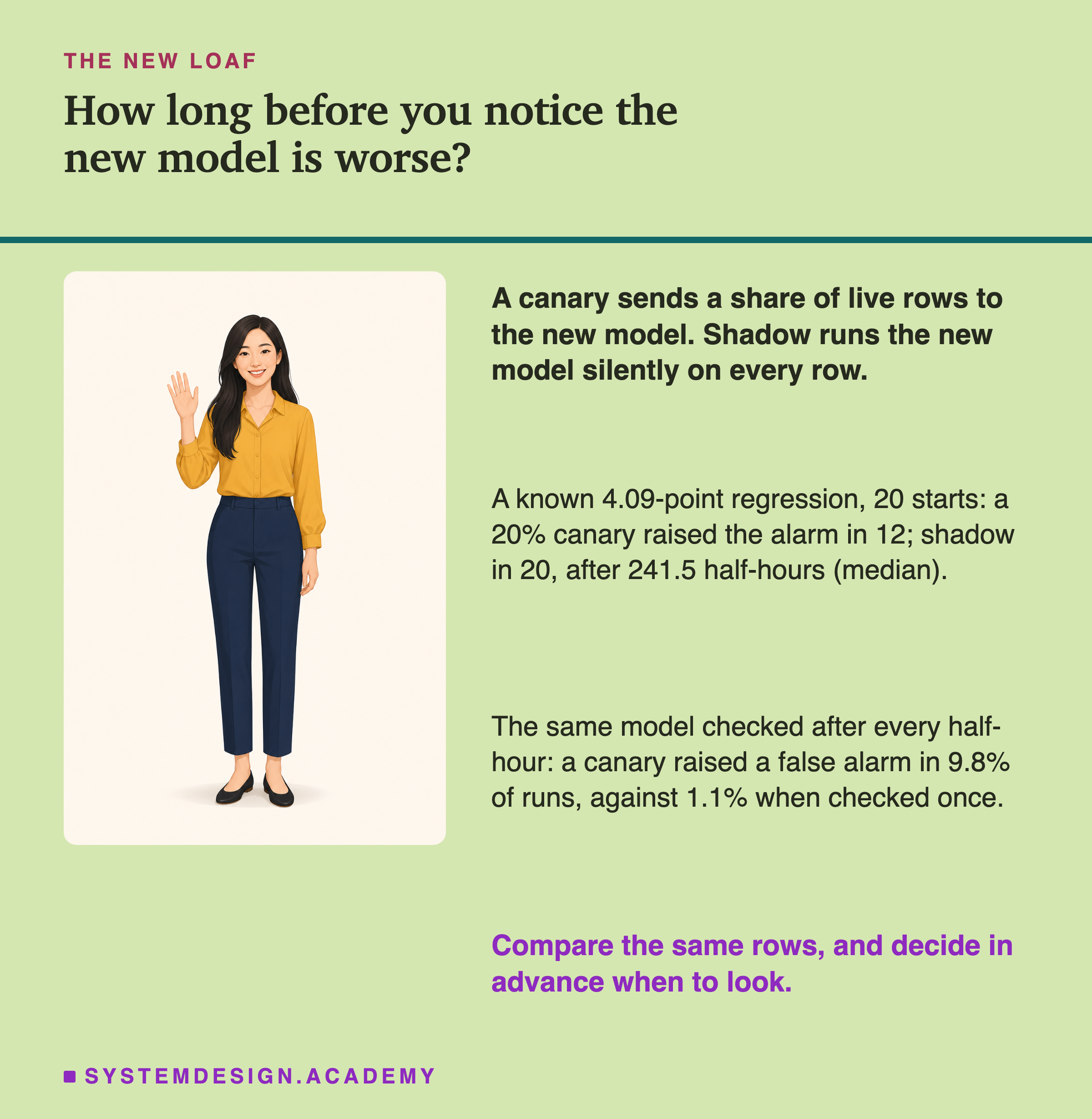
The second way: in every shop, bake both loaves for every order. The customer gets the old loaf, as always. A taster in the back tries both loaves from the same order and writes down which one is better. No customer ever eats the new loaf, so no customer is harmed. And because the taster compares two loaves made for the same order, the fussy school children and the busy office workers no longer spoil the comparison. The cost is simple to see: the bakery bakes twice as much bread, and the taster's opinion is not the same as a paying customer's.

Both ways have a delay. A complaint arrives the next day, not at the counter. So the baker has to wait for the answers, and she has to decide how often to look at them. This lesson measures both ways for a program that learns from examples, and asks how long each one takes to notice that the new version is worse.

This chapter follows one model through its life on the same data. Start with the dumbest model set the baselines. Same code, different model showed that two runs of the same code give two different models. Picking the best of many showed that the winner of a big search can do worse on later months. The promotion gate measured how a new model is judged against the old one on stored rows, and found that a test which looks only at the rows where the two disagree held its false promotions near 5%, where "higher score wins" promoted equal models about half the time.

Now the new model has passed the gate, and it meets real traffic. The course's lesson on model serving and inference has a slide called "Shipping a New Version Without Betting All Your Traffic". It explains in words what a canary and a shadow rollout are, and in the middle of the slide it gives a short rule: shadow proves it is safe, canary proves it is better. I will not repeat it. One thing to add to that rule: when the right answer arrives for every row, shadow can also measure accuracy, and that is what this lesson measures. This lesson measures one question that slide does not: how many rows of live traffic each way needs before it can see that a new model is worse.

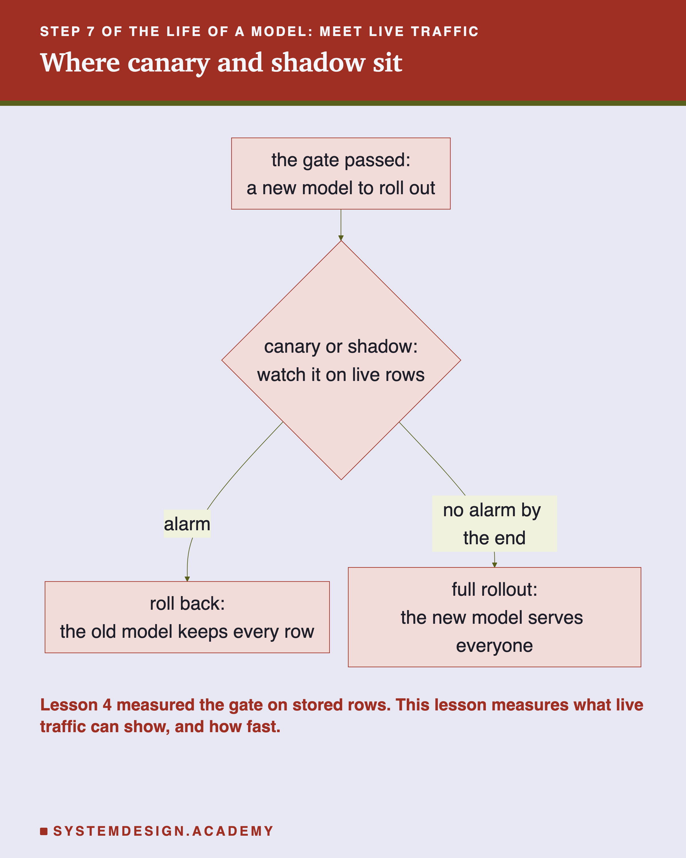
Why test on live traffic at all, if the gate already passed? Because the gate saw stored rows from the past, and live rows come from now. Lesson 3 found that months can differ a lot on this data. A model that passed on last season's rows can still be worse on this season's, and live traffic is the first place that shows.

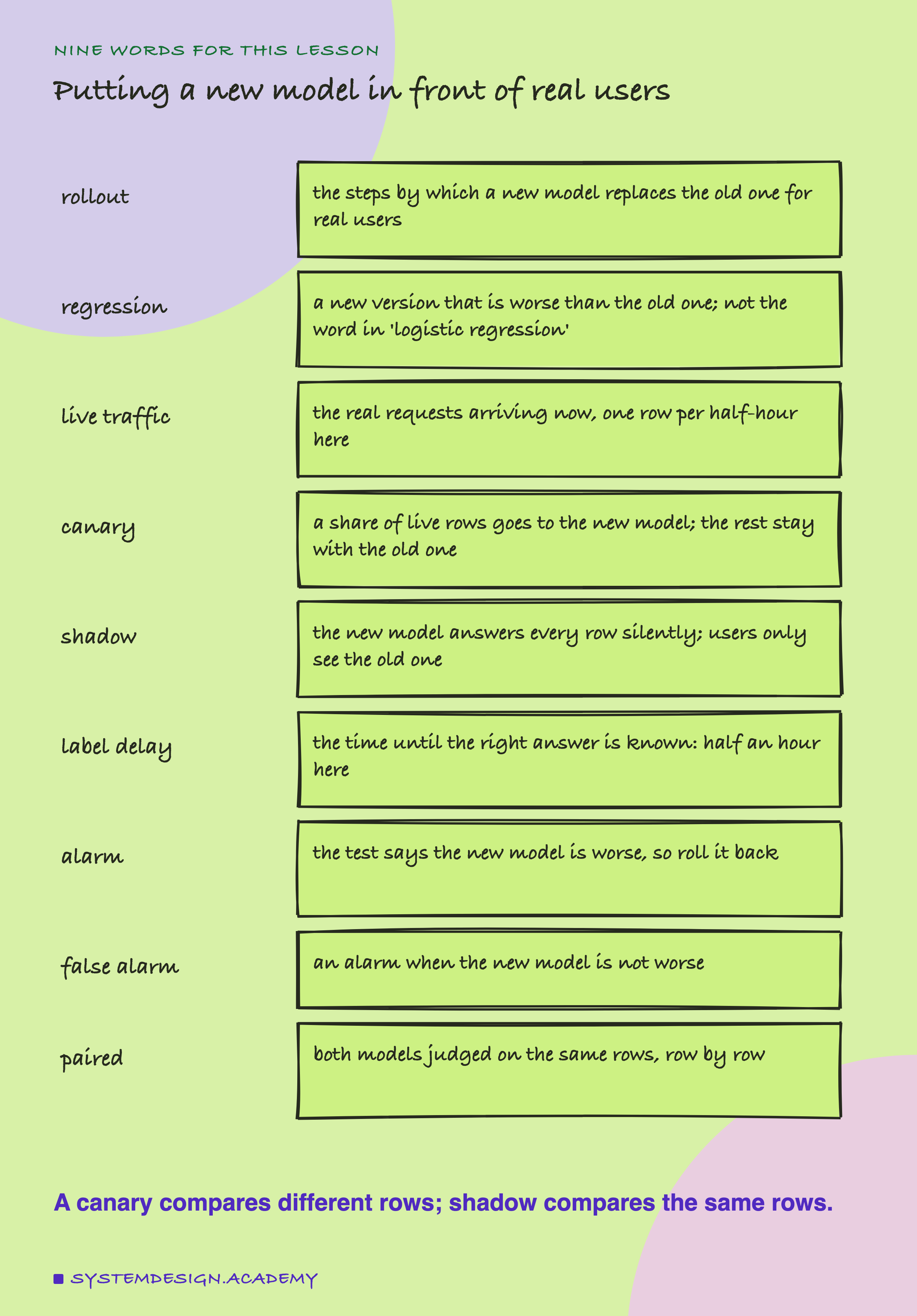
A rollout is the set of steps by which a new model replaces the old one for real users. To roll back is to send all traffic back to the old model. A regression is a new version that is worse than the old one. That is not the same word as the "regression" in "logistic regression", which is the name of a kind of model. This lesson uses both, and one of its challengers is both at once: the logistic regression model is the "big regression", because it is much worse than the champion. Live traffic is the stream of real requests arriving now. In this lab, one request is one half-hour of the electricity market, so the traffic is one row every half-hour. As in lesson 4, the old model that is live now is the champion and the new one is the challenger.

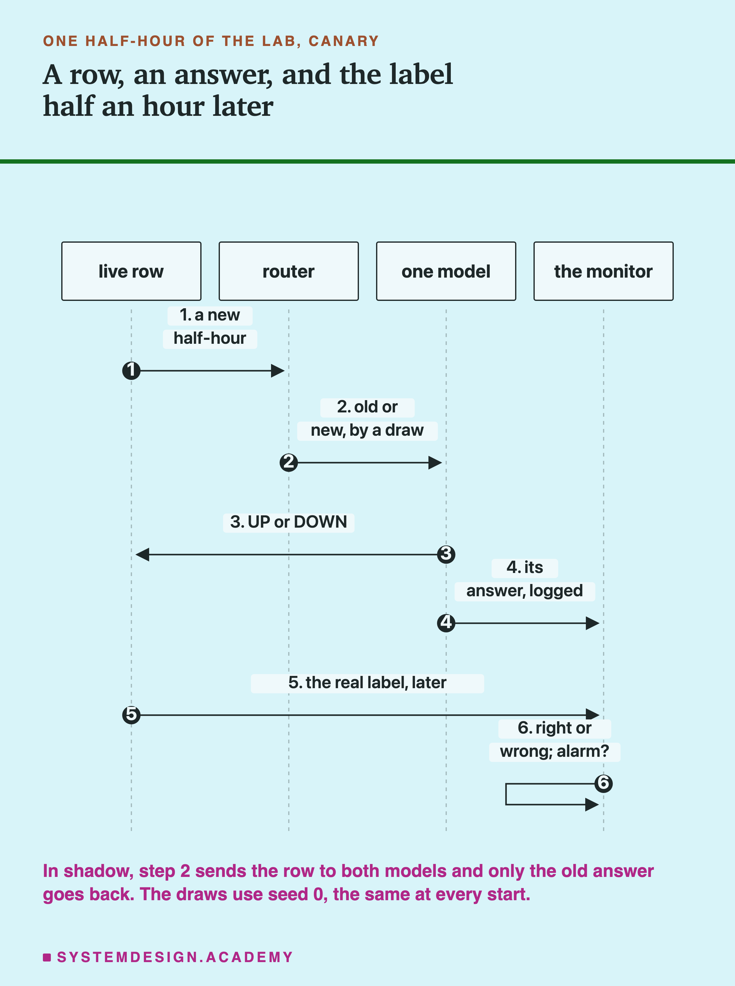
A canary rollout sends a share of live rows to the challenger, chosen at random, and keeps the rest on the champion. The name comes from the birds that miners once carried underground: if the air went bad, the small bird showed it first. A shadow rollout sends every row to both models. Users only ever see the champion's answer; the challenger's answer is written down and compared, never shown.

The label is the right answer for a row, and the label delay is how long it takes to arrive. Here, whether the price went UP or DOWN is known half an hour later. An alarm is the monitoring test saying "the challenger is worse, roll it back". A false alarm is an alarm when the challenger is not worse. A comparison is paired when both models are judged on the same rows, row by row. is the share of rows a model got right, and a is one hundredth of accuracy.

Here is the difference between the two rollouts on real rows. The sketch shows the first 16 live half-hours of the lab, with the lab's real random draw for a 20% canary and the real right-or-wrong outcomes of two models: the champion, which is boosted trees, and the logistic model from lesson 1, which is worse.

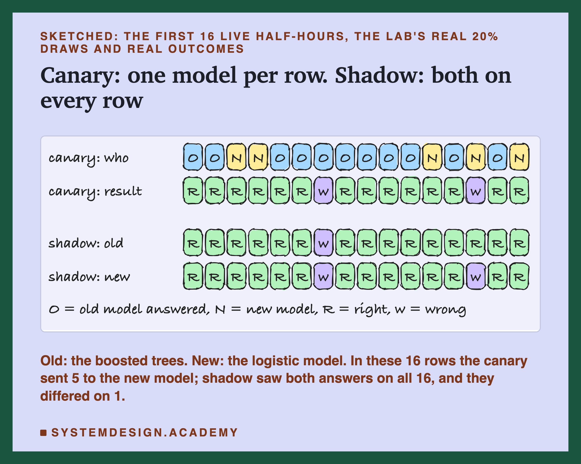
In the canary, each half-hour is answered by one model only. The draw sent 5 of these 16 rows to the new model. On each row, we learn how one model did, and never how the other would have done. To judge the new model, the canary compares its mistakes on its rows with the old model's mistakes on the other rows. Those are different half-hours, some easy and some hard.

In shadow, every half-hour is answered by both. On 15 of these 16 rows the two gave the same result, both right or both wrong. On one row, the fourteenth, only the old model was right. That single row is all the evidence these 16 half-hours hold about which model is better, and shadow sees it directly.

Look at the seventh half-hour. Both models got it wrong. In the canary, that row happened to go to the old model, so it counts as one mistake for the old model and tells us nothing about the new one. In shadow, it counts for neither, because the two agree. That is the whole idea of pairing, and the next slides measure what it is worth.

Each rollout needs a rule that turns the rows so far into a yes-or-no alarm. The lab fixed both rules in its file before it ran.

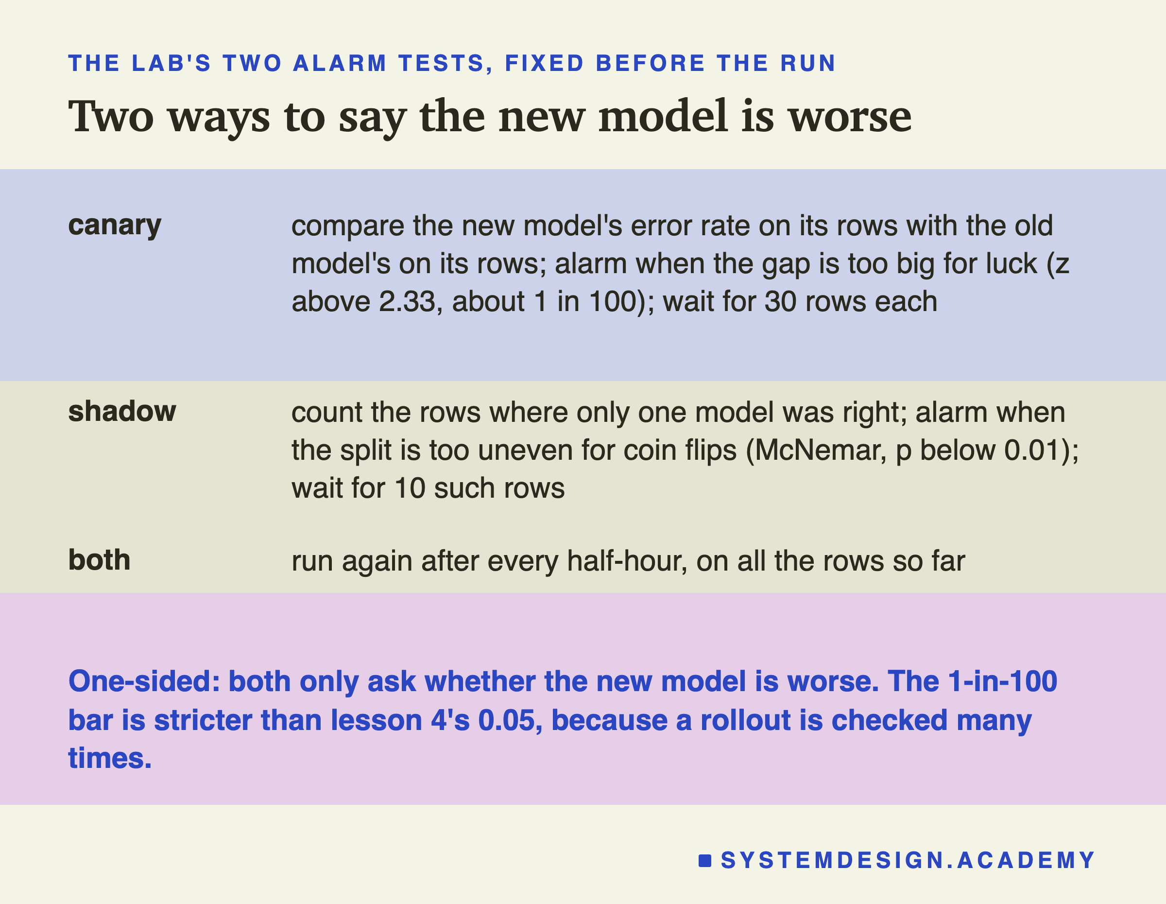
The canary test compares two error rates, the share of rows each model got wrong, measured on two different groups of rows. To judge the gap, it first puts both groups together and computes one pooled error rate, the share of all rows so far that were answered wrong. That pooled rate says how much two error rates on groups of this size would normally wobble by luck if the models were equal. The test asks how big the real gap is compared with that wobble. That ratio is called z. A z above 2.33 happens by luck about 1 time in 100 when the two models are equally good, so the lab sounds the alarm there. The test waits until each group has at least 30 rows, because with fewer rows the wobble is too wild to measure.

The shadow test is McNemar's test from lesson 4, turned around. It counts only the rows where exactly one model was right. If the two models were equally good, each such row would be a fair coin toss between them. The test asks how often fair coins would split this unevenly against the challenger. That chance is the p-value, and the lab sounds the alarm when it falls below 0.01, again about 1 in 100. It waits for at least 10 disagreeing rows. The bar of 0.01 is stricter than the 0.05 of lesson 4's gate, because a rollout is checked many times, and every check is another chance to be fooled.

Both tests are one-sided: they only ask whether the challenger is worse, because a rollout only rolls back in one direction. Both use the same 1-in-100 bar, so their false alarms can be compared fairly. And both were run again after every half-hour, on all the rows so far; a later slide measures what that does.

Before the results, here is the reason to expect shadow to be faster, and it has nothing to do with this lab.

A model's mistakes come from two things: the model, and the row. Some half-hours are simply hard. A price that jumps in a way the inputs could not foresee will fool almost any model. When a canary compares two error rates on different rows, both numbers carry the difficulty of their own rows. If the challenger's share of rows happens to hold a few more hard half-hours, it looks worse even if it is not. The canary has to wait until that luck of the rows averages out.

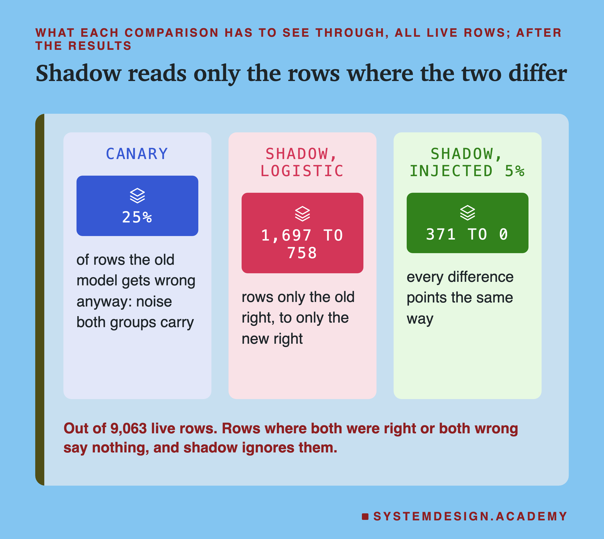
Shadow sees both models on the same half-hour. A hard row that fools both of them is a row where both were wrong, and it drops out of the test. So does an easy row both got right. What is left are the rows where the models truly behaved differently. On the 9,063 live rows, the champion got about 25% wrong. For the logistic model, the rows where only one was right numbered 1,697 against 758; for the injected challenger of the follow-up, 371 against 0. I counted these after the results. The canary has to find a difference hidden in the full 25% of noise; shadow looks at the difference itself.

This is the same point as the cafe customers in lesson 4 who liked both cups equally. They carry no information about which blend is better, and a paired test simply stops listening to them. The price of pairing is that both models must answer the same rows, which is exactly what shadow does and a canary cannot.

I wrote the lab's design at the top of its file, canary_lab.py, before it ran. The dated record is in the chapter plan (2026-09-29, "CANARY LAB (batch 5) designed before running").

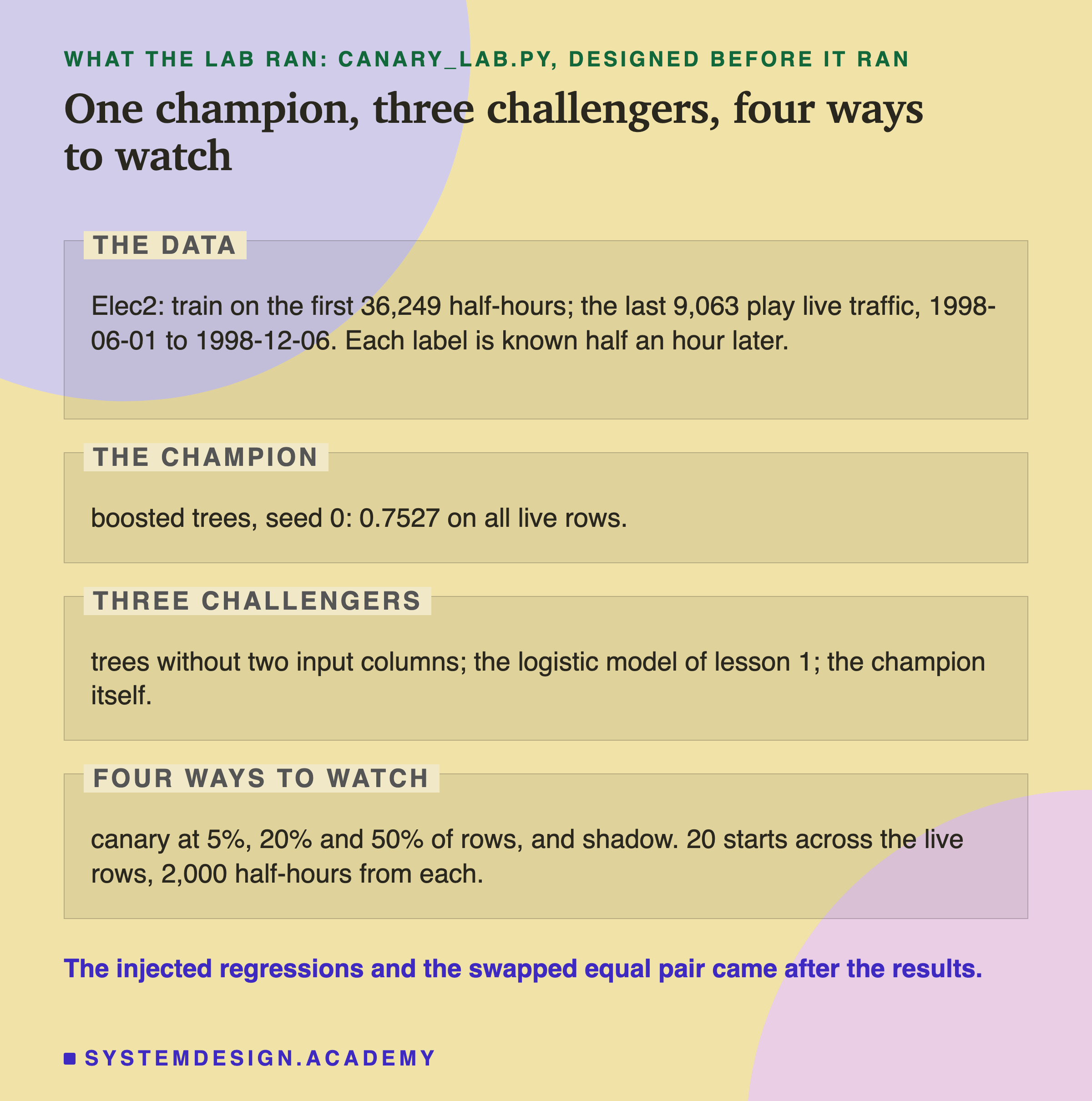
The data is Elec2 again: 45,312 half-hours of the New South Wales electricity market, May 1996 to December 1998, in time order. Each row asks whether the price is UP or DOWN against its average over the last 24 hours. The models train on the first 36,249 rows. The last 9,063, from 1 June to 6 December 1998, play the part of live traffic, one row per half-hour, and each row's label is known half an hour later, when the next row arrives.

The champion is the boosted trees with seed 0, the model of lessons 1 to 4. It scored 0.7527 on all the live rows. Three challengers were fixed in advance. A "small regression": the same trees trained without two inputs, vicprice and vicdemand, the price and demand in the neighbouring state of Victoria, as if a data pipeline had dropped two columns. A "big regression": the logistic model of lesson 1, about 10 points worse. And an "equal" challenger: the champion itself, so that any alarm would be a false one.

Here is what the lab stored in results/canary.json. For each challenger and each way of watching: in how many of the 20 starts an alarm came, and the median half-hour of the first alarm among those that came. The median is the middle value when they are lined up.

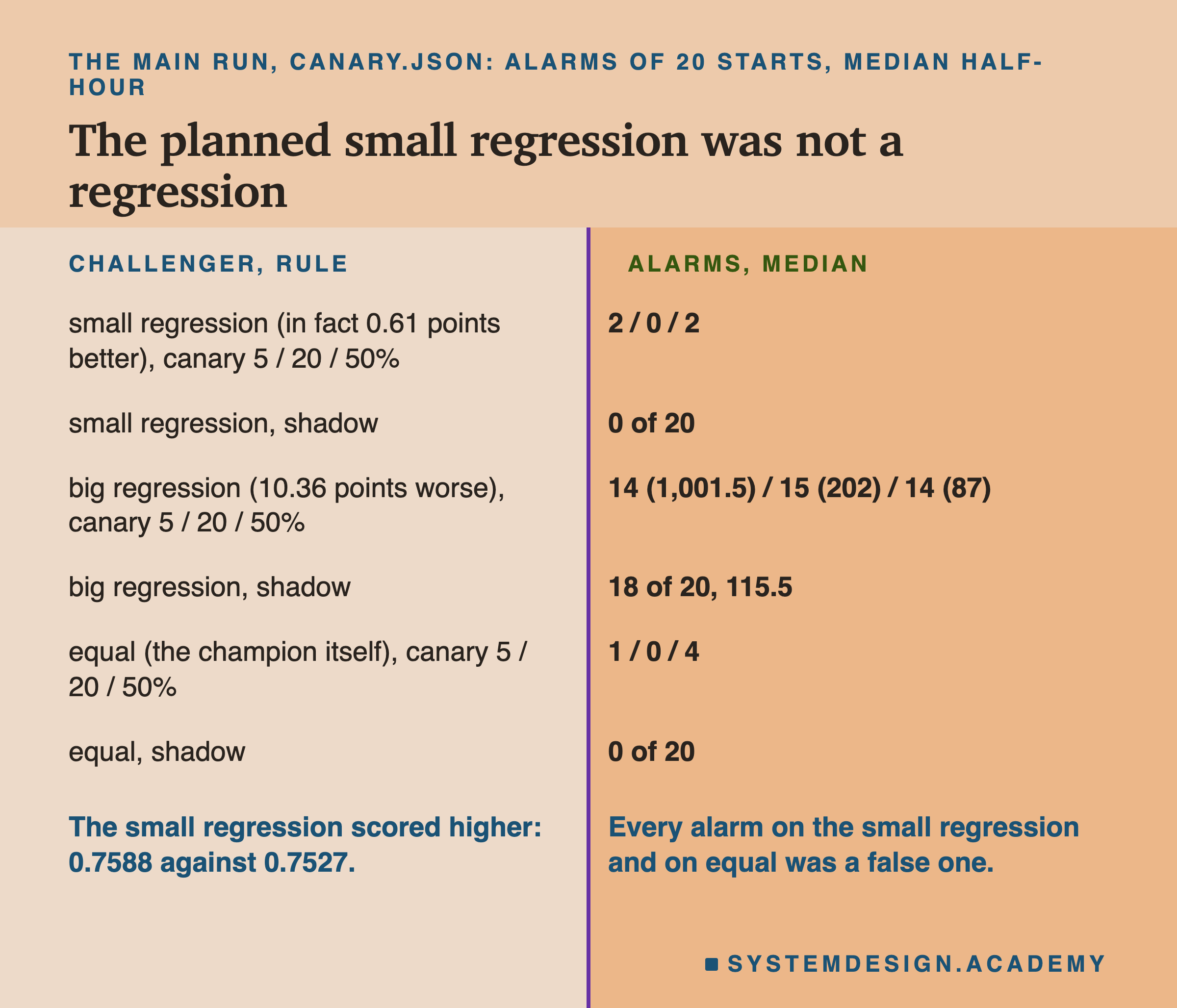
The big regression, 10.36 points worse over the whole live period, was caught by a 5% canary in 14 of 20 starts, with a median of 1,001.5 half-hours, about 21 days. A 20% canary caught it in 15, median 202 half-hours, about 4 days. A 50% canary caught it in 14, median 87 half-hours, under 2 days. Shadow caught it in 18 of 20, median 115.5 half-hours, about 2.4 days.

At first sight, a 50% canary looks faster than shadow: 87 against 115.5. A later slide shows that this comparison is misleading, because the two medians count different starts.

The small regression was not a regression. It scored 0.7588 on the live rows, 0.61 points above the champion. Dropping the two Victorian inputs made the trees slightly better here. Shadow never raised an alarm on it, which is correct. The canary did, twice at 5% and twice at 50%. In those starts the challenger was between 0.30 and 0.75 points better than the champion over the 2,000 half-hours, so these were false alarms against a model that was not worse. I measured those per-start gaps after the results.

The equal challenger, the champion itself, got 1, 0 and 4 false alarms from the canary. Shadow gave 0.

The main run answered some of what I asked, but two of my three challengers were built wrong, and I want them on the record rather than hidden.

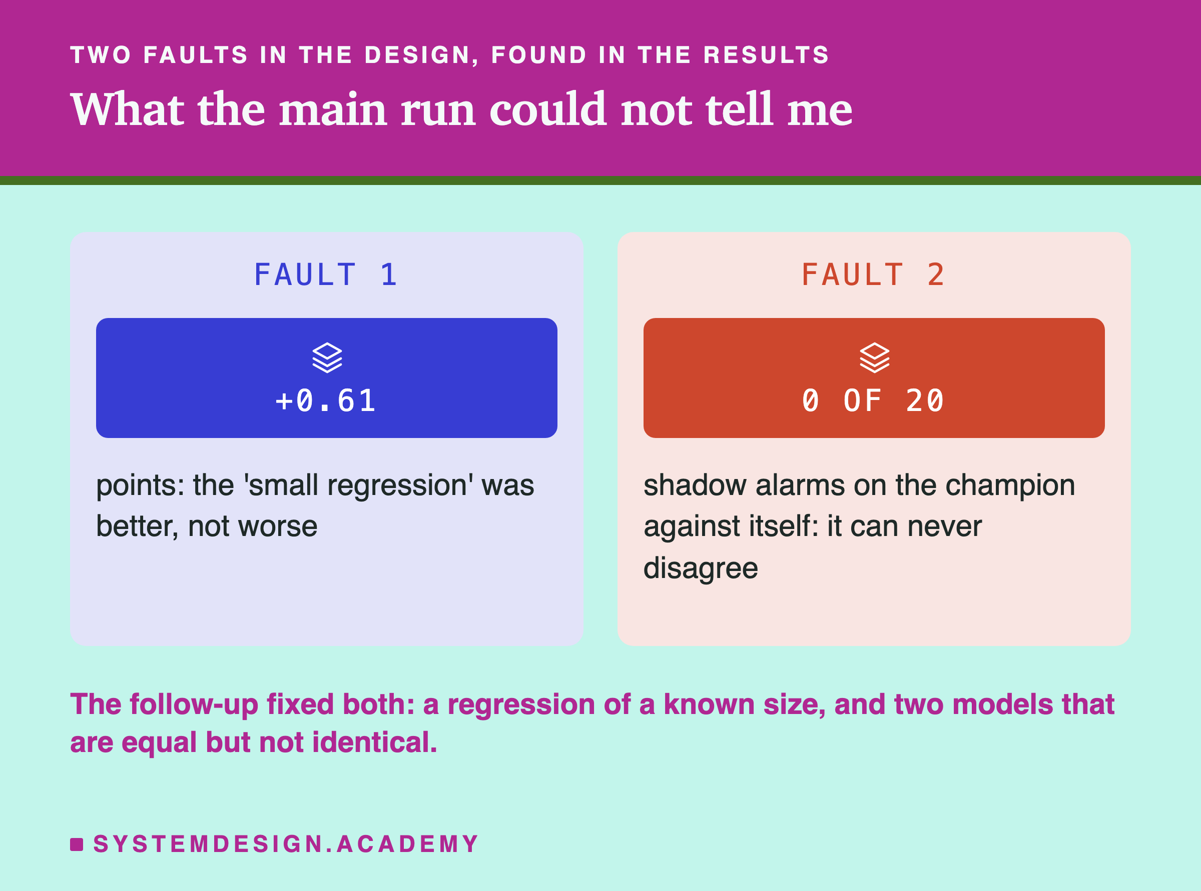
Fault 1: the small regression was not a regression. I guessed that removing two inputs would make the model a little worse, and wrote "its size is whatever the data gives" into the design. The data gave a model 0.61 points better. So the main run has only one real regression, the logistic model, and no small one. Its question, "how much traffic does it take to see a small regression?", was left without an answer.

Fault 2: the equal challenger made shadow's zero meaningless. I used the champion itself as the equal challenger, so its answer matched the champion's on every row. For a canary that is a fair test: the two groups are still different rows, so luck can still make one look worse, and the 1, 0 and 4 false alarms are real. But shadow counts only the rows where the two models disagree, and here there were none. Shadow could not have raised an alarm whatever its rule. Its 0 of 20 says nothing about how often shadow raises false alarms.

So I designed a follow-up after I saw the main results, and I wrote its design into the lab file's followup mode before it ran. It fixed both faults. For regressions of a known size, it took the champion's own live results and gave each right answer a 2% or 5% chance of being turned wrong. For an equal pair that can disagree, it used lesson 4's trick: two seeds of the trees, with their results swapped row by row by a coin, so that neither can be better by design. Its results are in results/canary_followup.json.

Before the follow-up, the main run's one real regression deserves a closer look, because its 20 starts are not alike. After the results, I measured how far the logistic model was behind the champion inside each start's own 2,000 half-hours.

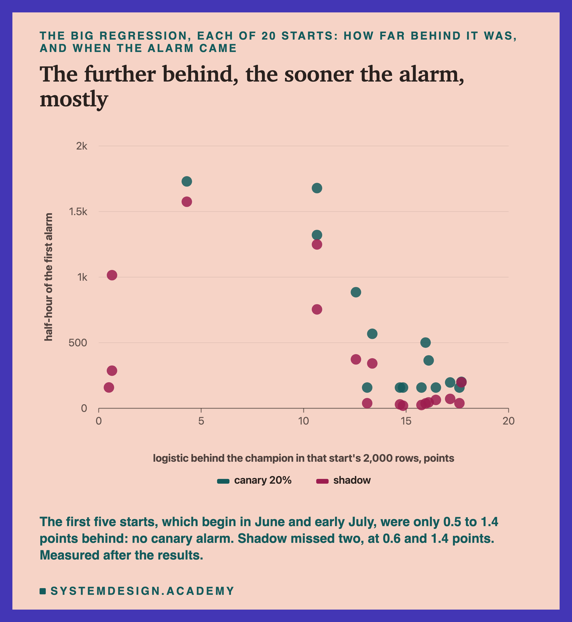
The "10-point regression" is an average over the whole live period, and it hides a lot. In the first five starts, which begin in June and early July, the logistic model was only 0.5 to 1.4 points behind over its 2,000 half-hours. In the last fourteen starts it was 10.7 to 17.7 points behind. No canary of any size raised an alarm in the first five starts. Shadow raised one in three of them and missed the other two. In the late starts, where the gap was large, everything saw it, and shadow saw it first.

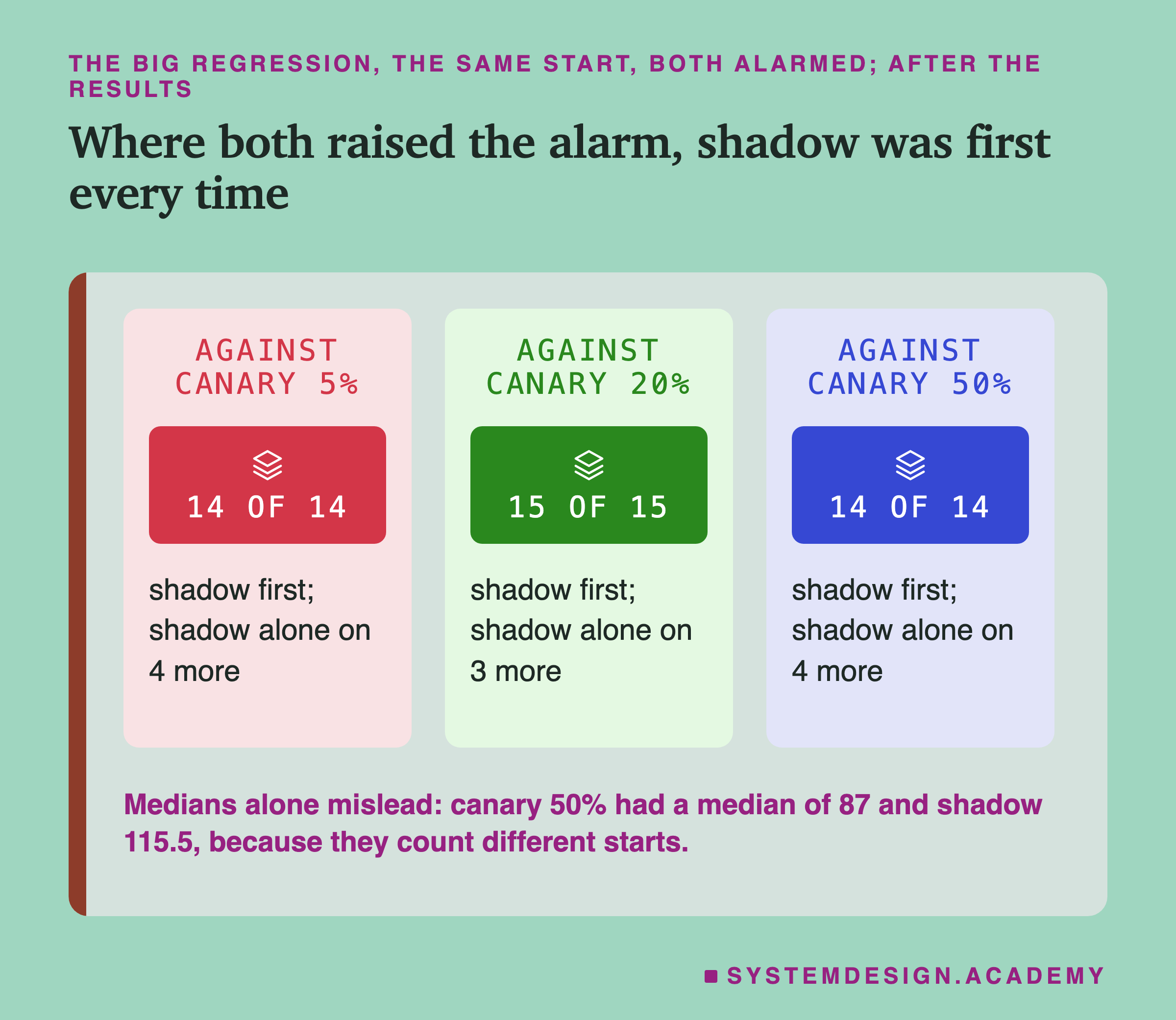
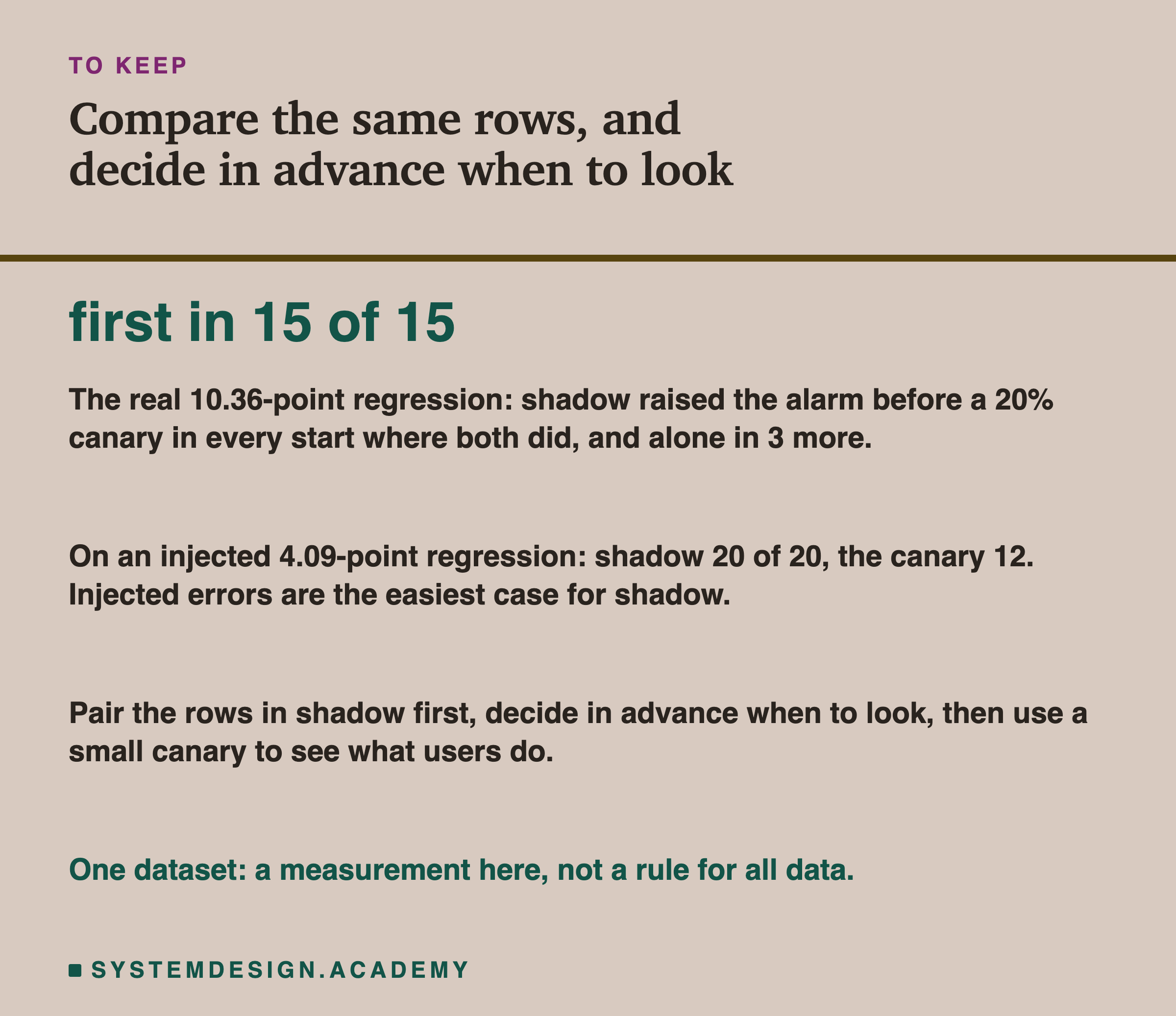
This explains the strange medians. The 50% canary's median of 87 half-hours comes only from the 14 starts where it caught anything, and those were the late starts with a big gap. Shadow's median of 115.5 includes slow catches from the early starts, where the canary caught nothing at all. Compared start by start, which I did after the results, shadow was first in every start where both raised an alarm: 14 of 14 against the 5% canary, 15 of 15 against 20%, and 14 of 14 against 50%. It was never second.

The lesson for reading any rollout report: a median of "time to alarm" means little unless you know which runs had an alarm. A method that only catches the easy cases can post a faster median than one that catches everything.

The follow-up gives two regressions whose size is known exactly. Each of the champion's 6,822 right answers on the live rows had a 2% or a 5% chance of being turned wrong. The draw turned 159 of them (2.3%) and 371 (5.4%), which made challengers 1.75 and 4.09 points worse. I counted those after the results. The same 20 starts, the same four ways of watching, the same alarm tests.

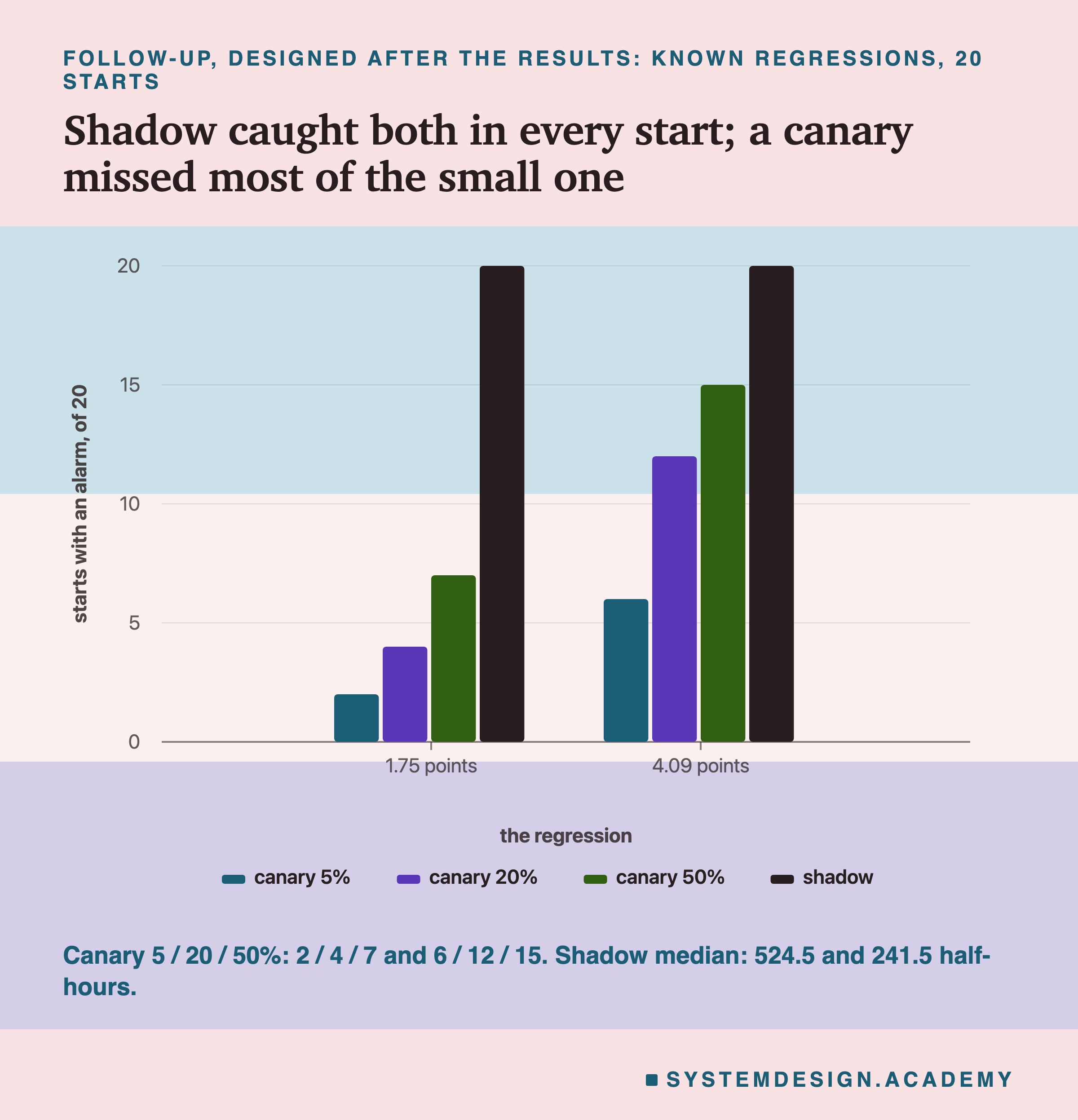
The 1.75-point regression: the canary raised an alarm in 2, 4 and 7 of 20 starts at 5%, 20% and 50%. Shadow raised one in all 20, with a median of 524.5 half-hours, about 11 days. The 4.09-point regression: the canary in 6, 12 and 15 of 20; shadow in all 20, median 241.5 half-hours, about 5 days.

The equal pair, two seeds with their results swapped by a coin, came out 0.08 points apart over the live period, which is as close to equal as real models get. The canary raised false alarms in 1, 0 and 2 of 20 starts. Shadow raised none. This time shadow's zero means something, because these two models did disagree: on 325 of the 9,063 live rows, and the swap made each such row a fair coin.

Start by start, again after the results: against the 4.09-point regression, shadow alarmed first in 6 of the 6 starts where the 5% canary also alarmed, 11 of 12 at 20%, and 11 of 15 at 50%. So a big canary sometimes beat shadow to the alarm here, which never happened with the logistic model. But in every case the canary missed starts that shadow caught: 14, 8 and 5 of them.

Twenty out of twenty, twice, is an unusually clean result, and an unusually clean result means inspect the inputs first. So I did, after the results.

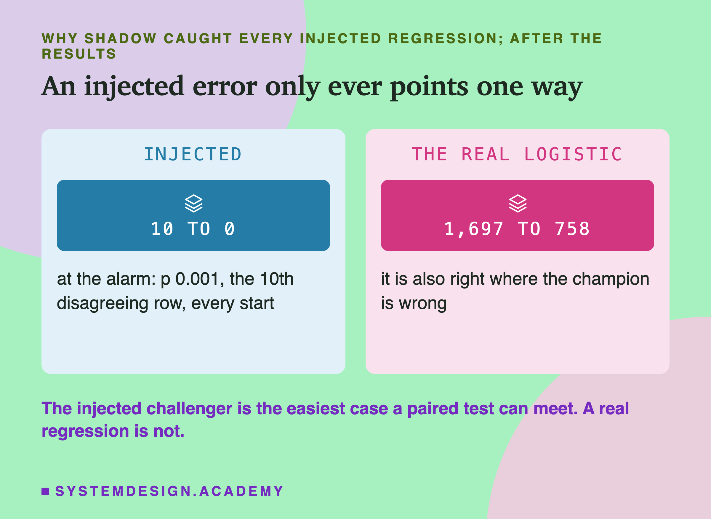
The injected challenger was built from the champion by turning some right answers into wrong ones. It never turns a wrong answer into a right one. So on every row where the two disagree, it is the champion that is right. The split of disagreeing rows is always "all of them to the champion, none to the challenger". For McNemar's test, that is the most lopsided split possible: the chance of 10 fair coins all landing the same way is 0.5 to the power 10, about 0.001. The alarm fired at exactly the 10th disagreeing row in every start, for both injected regressions; the test was only waiting for the 10-row minimum. The report checks this for all 40 alarms.

A real worse model does not behave like that. The logistic model was right on 758 live rows where the champion was wrong, against 1,697 the other way. Its disagreements point both ways, so shadow has to wait for the uneven split to build up. That is why shadow took a median of 115.5 half-hours on the logistic model and missed two starts, while a much smaller injected regression was caught every time.

So the follow-up's shadow numbers are the best case for a paired test. They show how fast shadow can be when every disagreement is a real loss. They do not show how fast it is on a real regression of 4 points; that would depend on how often the real challenger also wins some rows. The canary's numbers are affected much less, because the canary never looks at disagreements: it compares error rates, and a 4.09-point rise in errors is a 4.09-point rise however it was made. That last point is reasoning, not a measurement: errors that bunch up in time could still change what a canary sees.

The injected errors were scattered at random, one row here, one row there. A real regression might not be. It might be fine for weeks and then fail badly when the weather or the market changes. That matters because a test that counts rows as separate coin flips assumes they are scattered. So I measured it on the stored outcomes, after the results.

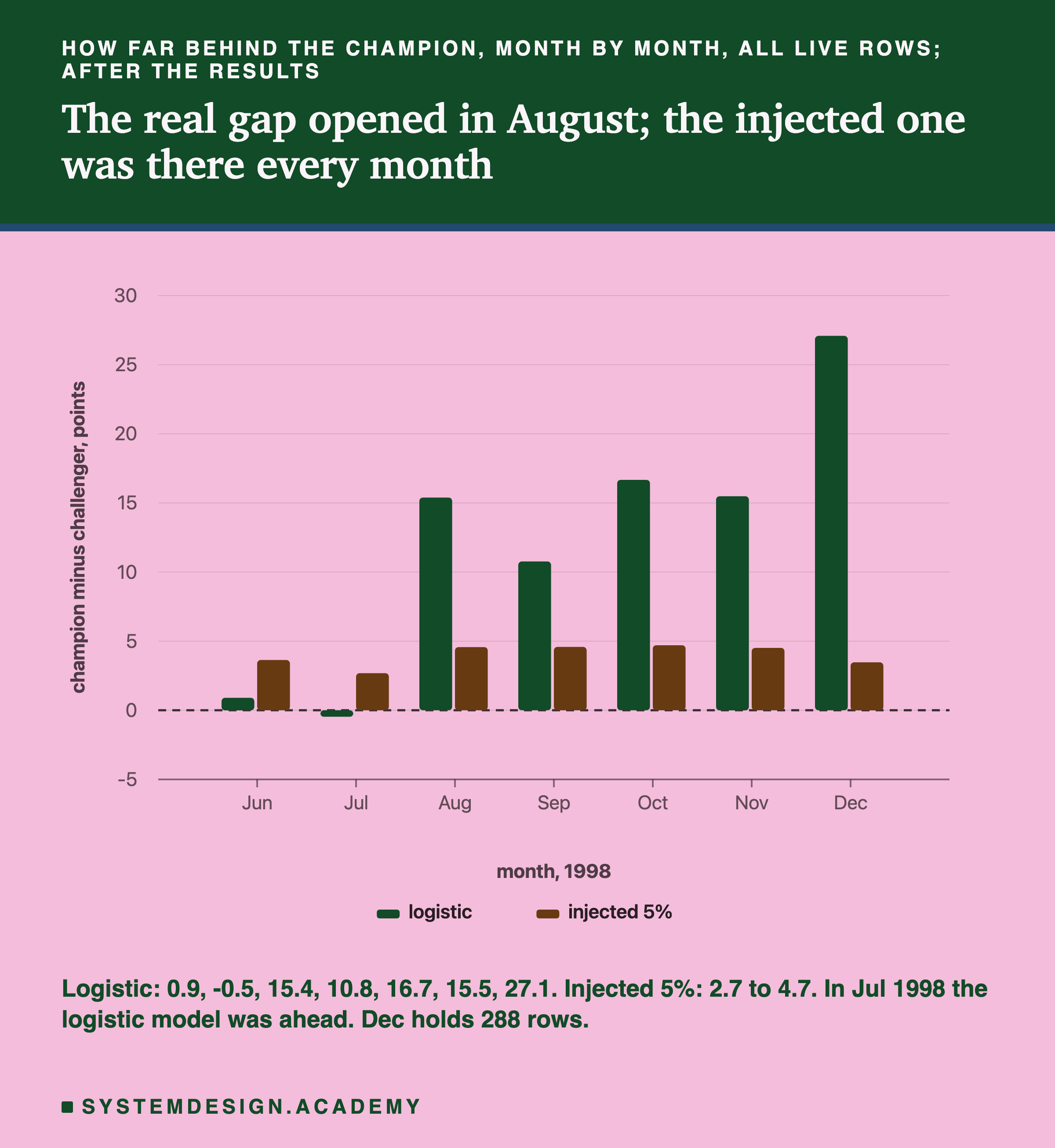
It does bunch up. Month by month, the logistic model was 0.9 points behind the champion in June and 0.5 points ahead in July. Then the gap opened: 15.4 points in August, 10.8 in September, 16.7 in October, 15.5 in November and 27.1 in the six days of December. The injected 5% regression was 2.7 to 4.7 points behind in every month, as you would expect from errors thrown in at random. The injected 2% was 1.0 to 2.1.

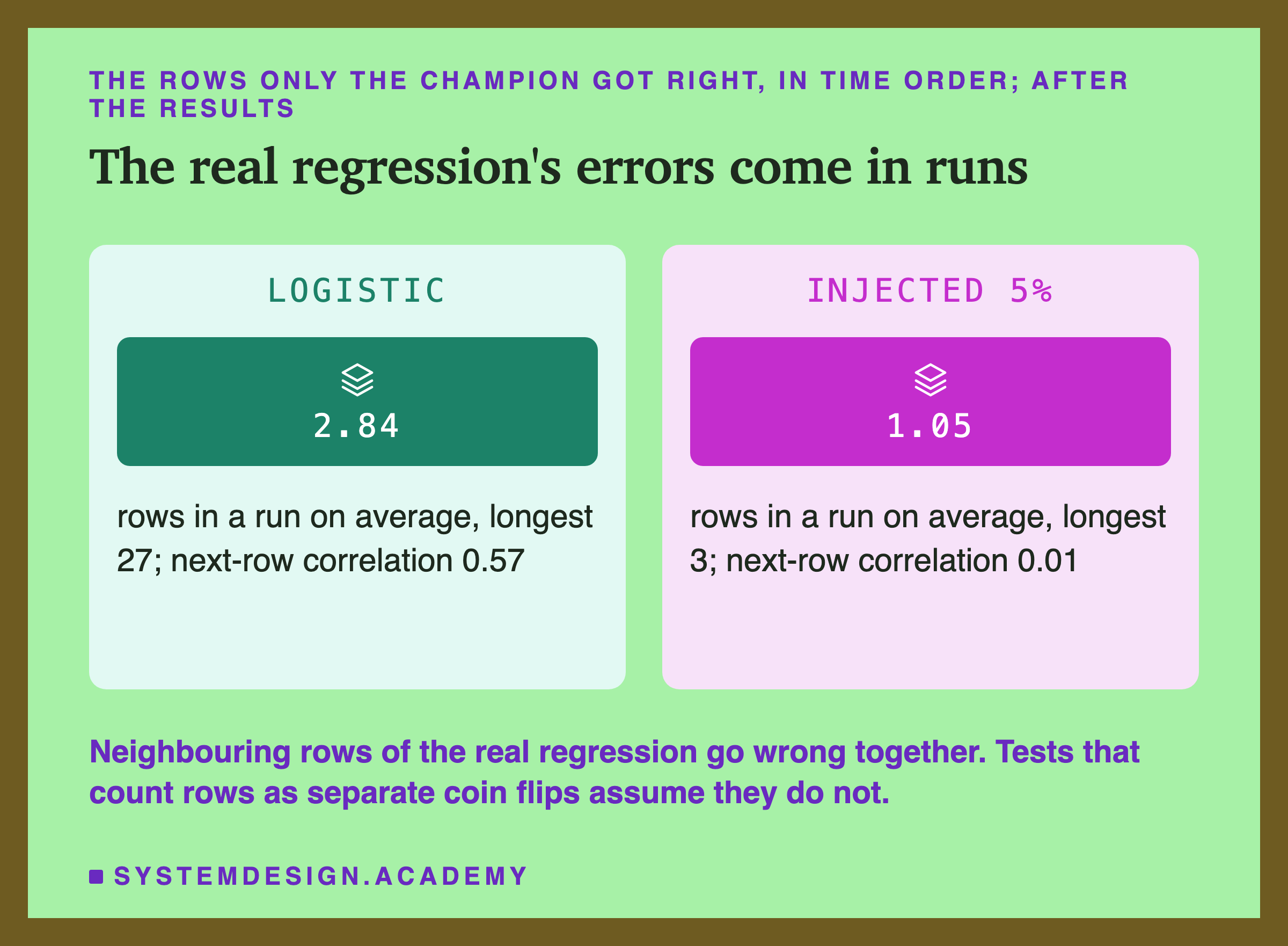
It bunches up row by row too. Take the rows where only the champion was right, in time order. For the logistic model, those 1,697 rows came in runs of 2.84 rows on average, the longest 27 in a row, and whether one half-hour was such a row predicted the next one strongly: a correlation of +0.57, where 0 means no link and 1 means always the same. For the injected 5% errors, the runs averaged 1.05 rows and the correlation was +0.01, which is no link at all.

Why did the logistic model fall behind from August? I measured that it did, not why. One possible reason, and it is a guess I have not tested: something in the inputs changed from August in a way the straight-line model handles worse than the trees. Lesson 3's comparison of months cannot settle it, because its later months include June and July, when the logistic model was fine. What the measurement does settle is the caveat the follow-up needed. Random injected errors suit a paired test that treats rows as separate coin flips. A real regression came in runs and in seasons, and a test that assumes separate coin flips may be too sure of itself on such rows. This lab did not measure how much.

There is a simpler reason a small canary is slow, and it is plain counting. I counted it after the results, from the lab's own random draws.

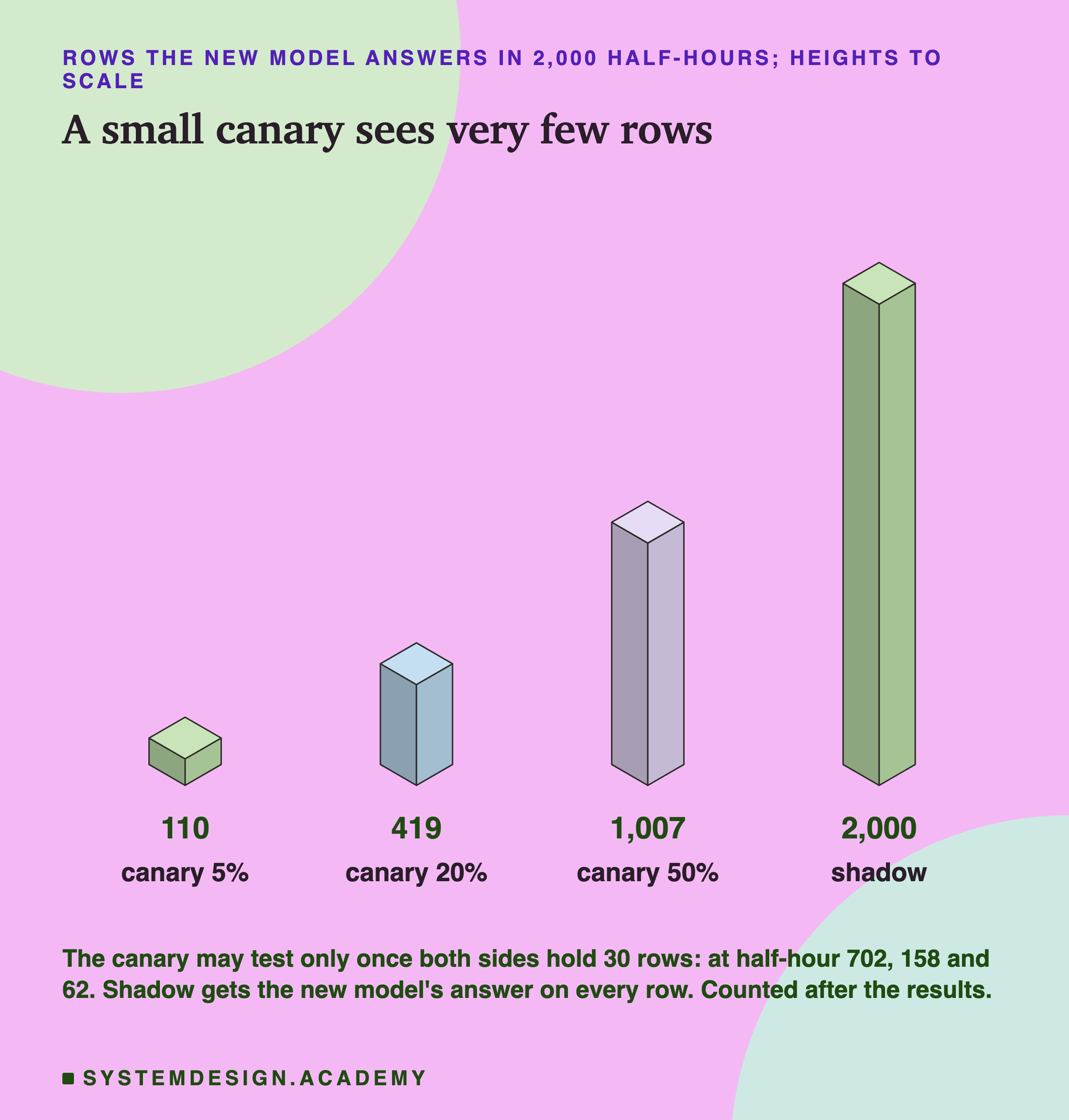
In 2,000 half-hours, almost 42 days, a 5% canary sent just 110 rows to the challenger. A 20% canary sent 419, a 50% canary 1,007. Shadow gets the challenger's answer on all 2,000. A canary's test needs rows from both models, and the fewest it gets are from the challenger. With 110 rows, the error rate of the challenger is only known to within several points either way, so only a large regression can be told apart from luck.

The 30-row minimum has a second effect. A 5% canary reached 30 challenger rows only at half-hour 702, almost 15 days in; a 20% canary at 158; a 50% canary at 62. That first allowed test is also the one with the fewest rows, when luck swings the most. Of the big regression's alarms, 5, 6 and 5 fired at that very first allowed check. The same first check shows up over and over in the table of starts, because the lab used the same random draw at every start. That was a simplification of my design, and a reason the 20 starts are less independent than they look.

This is where the real world differs most from this lab. Elec2 has one row per half-hour. A real service may get thousands of requests a minute, so a 5% canary could see 110 labelled rows within minutes. What matters is not the clock but the number of labelled rows each model has answered. The numbers in this lesson are in half-hours because that is how the data arrives; read them as rows.

Both alarm tests were run again after every new half-hour, on all the rows so far. Lesson 4 measured what repeated checking does to a promotion gate: on equal models, checking after every 200 rows turned 2 false promotions out of 20 into 6. Monitoring a rollout is exactly the case where a team wants to look at every new batch, so I measured it here too, after the results.

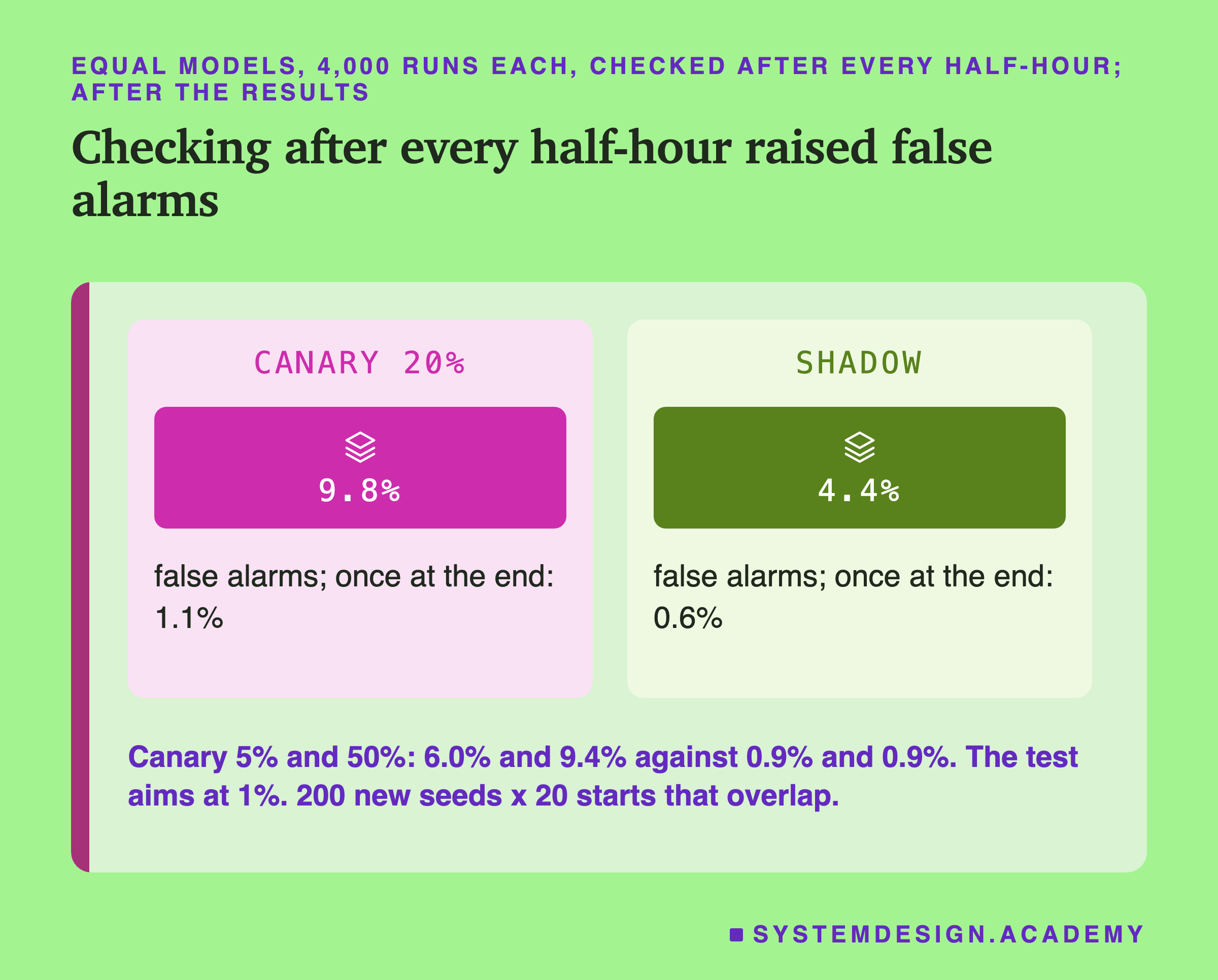
For the canary I ran the champion against itself, which is a true null for a canary because the two groups are still different rows, with 200 new random draws at each of the 20 starts: 4,000 runs per share. For shadow I used the swapped pair of seeds with 200 new coins, also 4,000 runs. Each run was tested two ways: after every half-hour, and once, at the end of the 2,000.

Tested once at the end, the false alarms landed where the 1-in-100 bar says they should: 0.9%, 1.1% and 0.9% for the three canaries and 0.6% for shadow. Tested after every half-hour, they rose to 6.0%, 9.8% and 9.4% for the canaries and 4.4% for shadow. So watching continuously multiplied the false alarms by about seven to eleven: 6.9, 8.9 and 10.7 times for the three canaries, and 7.0 times for shadow. Shadow's rates were lower only in absolute terms; its ratio was the same as the 5% canary's. One likely reason its rates are lower, which is reasoning rather than a measurement: with few disagreeing rows an exact test cannot land exactly on its bar and stays below it, 0.6% here when checked once, against the 1% it aims at.

The swapped pair also makes shadow's side a best case. The coin makes every disagreeing row a fair and separate toss, which is exactly what McNemar's test assumes. Real equal models whose disagreements come in runs, like the logistic model's errors, could give shadow more false alarms than 4.4%, and this lab did not measure how many.

This also explains the main run's false alarms. The canary's 1, 0 and 4 false alarms on the equal challenger, and the 2 and 2 against a slightly better model, all came from checking after every half-hour. The 4,000 runs are not independent: the 20 starts overlap, and neighbouring starts share about 81% of their rows. For the canary I also counted where those false alarms fired: 50 of 240, 49 of 391 and 35 of 375 came at the very first allowed check (21%, 13% and 9%), and the rest a median of 322, 267 and 220 half-hours after it. Read the rates as a clear direction, not as exact values.

Shadow looks better on every measurement so far. It is not free, and its costs are of a different kind from the canary's.

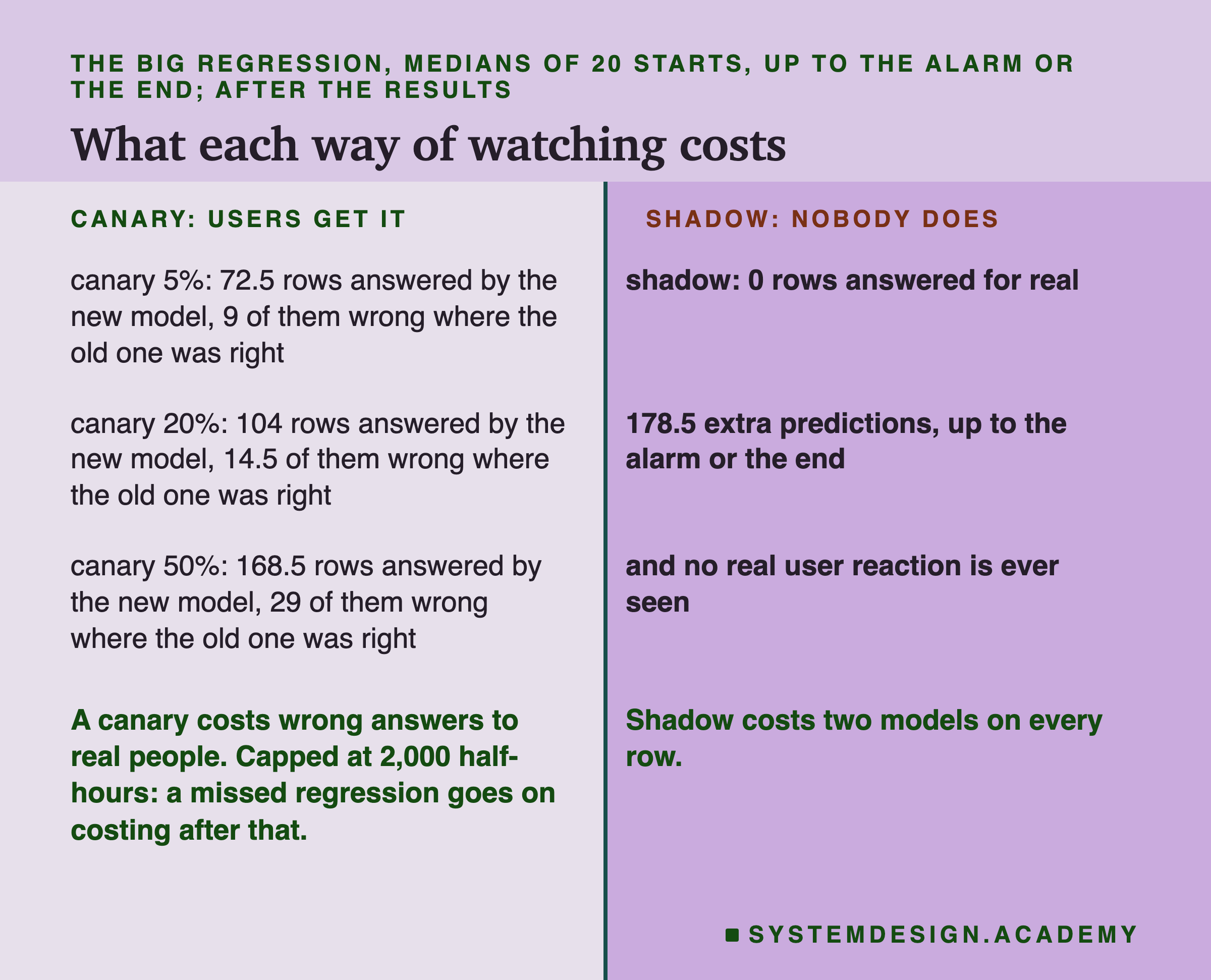
A canary's cost is paid by users. Every row the challenger answers is a real answer to a real person. With the big regression, I counted after the results how many rows the challenger answered before the alarm, or before the end of the 2,000 half-hours when no alarm came, and how many of those it got wrong where the champion would have been right. The medians over the 20 starts: 72.5 rows and 9 extra wrong answers for a 5% canary, 104 and 14.5 for 20%, 168.5 and 29 for 50%. A bigger canary sees the problem sooner, and hurts more people while it does.

These counts stop at 2,000 half-hours. A regression the canary missed goes on giving wrong answers after that, for as long as the rollout runs, so the counts make a small canary look cheaper than it is.

Shadow's first cost is compute. Every row is answered twice. Counted the same way as the canary, up to the alarm or to the end of the 2,000, shadow ran a median of 178.5 extra predictions on the big regression. For small boosted trees that is nothing. For a large model that needs an expensive graphics card for each answer, running two copies on all traffic can double what the service costs to run, and many teams shadow only a sample of traffic for that reason.

Shadow's second cost is blindness. The challenger's answers are never shown, so nothing a user does in reply to them is ever seen. In this lab that does not matter: the price goes up or down whatever the model says. In a real product it often does matter. A recommendation changes what people click; a fraud score changes which payments go through; a search ranking changes what people read. Those effects only exist when real people get the new answers. Shadow can show that a model is less accurate on the same rows. Only a canary can show what users do with it.

Here is what the lab points to, in the order a rollout meets it.

Start in shadow, and pair the rows. Run the challenger on every live row next to the champion, and compare them only on the rows where exactly one was right. On every regression in this lab, shadow raised the alarm in more starts than any canary, and on the real one it was first in every start where both did.

Count labelled rows, not hours. Before a rollout, work out how many labelled rows each model will answer per day. A 5% canary here saw 110 rows in almost 42 days, which could only see a very large regression. If a canary is too small to see the regression you care about, it is only a slow way of harming a few users.

Decide in advance when to look. Choose the points at which you will test, and test only there, or use a method built for repeated looks, which demands a stricter bar at each look. Here, testing after every half-hour turned a 1% false-alarm rate into 6 to 10% for a canary.

Be careful with the first look. The first test a canary may run is the one with the fewest rows. Here more than a third of the big regression's canary alarms fired at that very first check: 5 of 14, 6 of 15 and 5 of 14. A real regression that big deserves the alarm. For false alarms, the first check is a single look on the fewest rows: in the 4,000 runs on equal models it held 21%, 13% and 9% of the canary's false alarms, and none of the lab's own 12.

Look at time slices, not only the total. The logistic model was a 10-point regression on average, and less than 1.5 points behind in the starts that began in June and early July. A canary that ran in June would have passed it; shadow caught it in 3 of the 4 June starts. If your data has seasons, watch long enough to cover the ones that matter.

Then use a canary for what only a canary can see. Once shadow shows no accuracy problem, a small canary is the way to see how real users respond. Keep it small, keep the old model ready to take all traffic back, and log every alarm with the rows and counts behind it, next to the gate record of lesson 4.

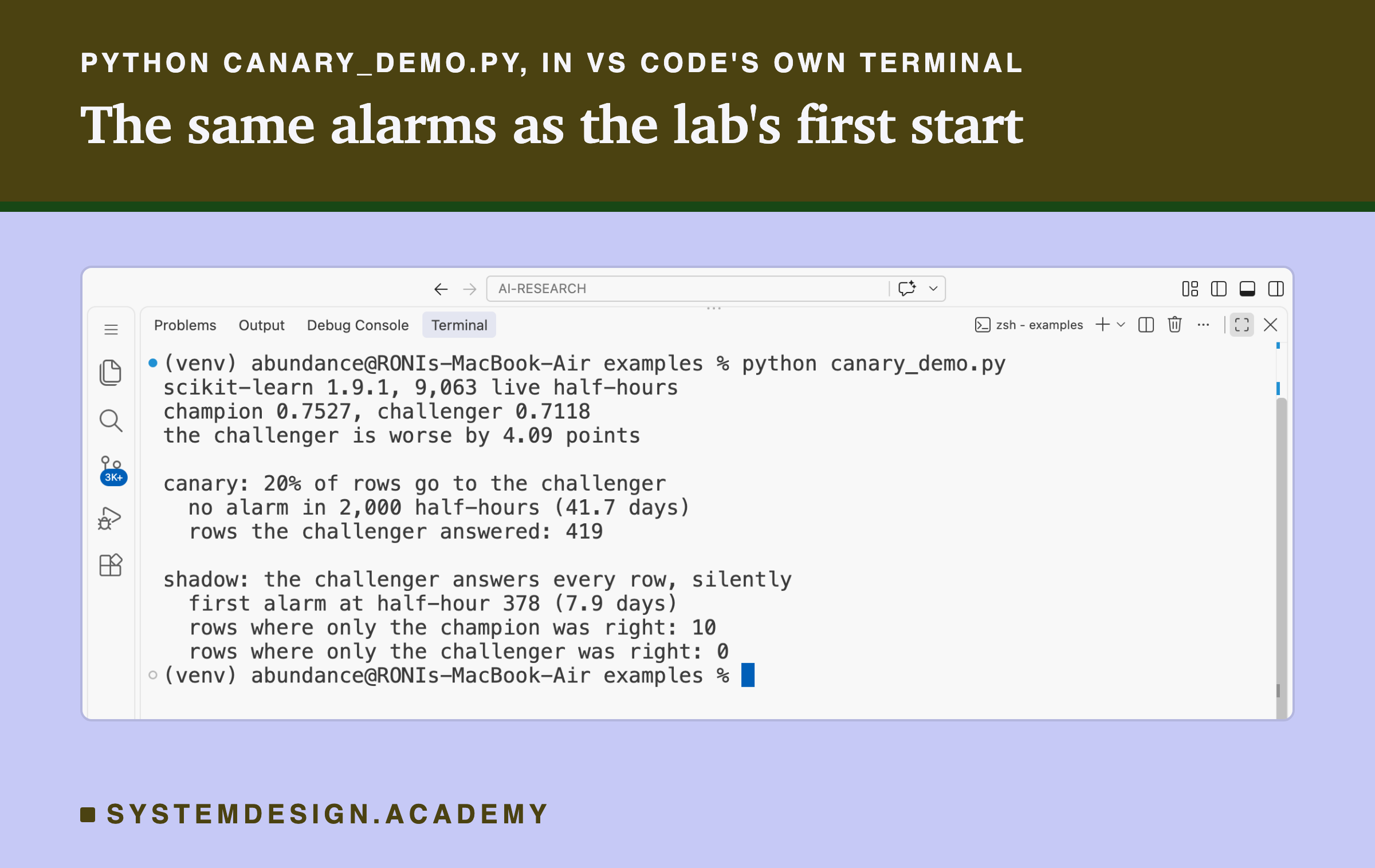
This script is the lab made small. It downloads the same data, trains the champion, builds the known 4.09-point regression exactly as the follow-up did (its comment says 5% of the right answers; each one had a 5% chance, and 5.4% were turned), and then watches the first 2,000 live half-hours twice: once as a 20% canary, and once in shadow. It prints the half-hour of each first alarm, or says that none came. It does not need a GPU.

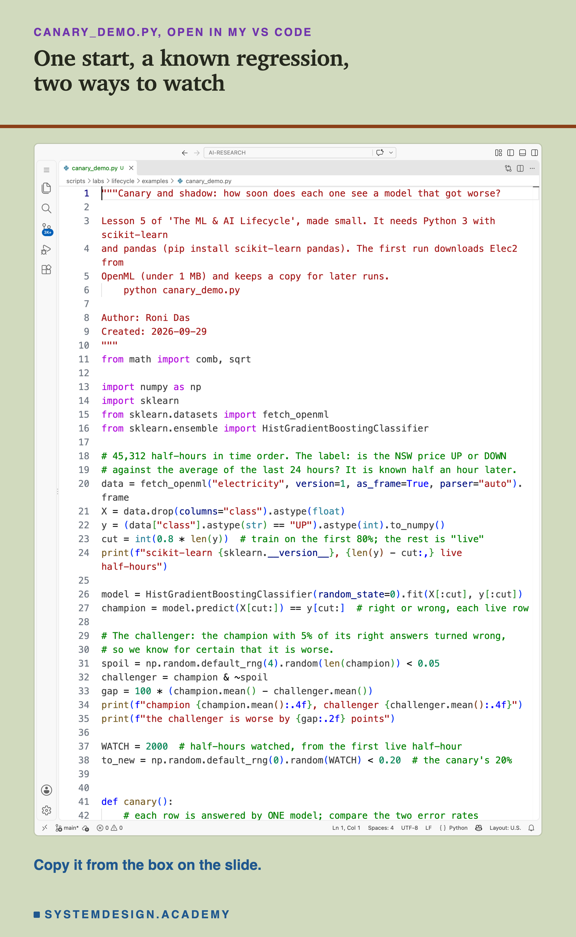
Before you run this lab. You need Python 3 and two libraries: pip install scikit-learn pandas. scikit-learn holds the model and the download, and brings NumPy with it; pandas holds the table. The first run downloads Elec2 from OpenML (under 1 MB compressed), so it needs an internet connection once; scikit-learn keeps a copy in a folder in your home directory (scikit_learn_data) for later runs. Both alarm tests need no extra library: they are a few lines of arithmetic with Python's own math. I ran it with scikit-learn 1.9.1 on a Mac. scikit-learn runs the same way on Windows and Linux, but I have not checked the numbers there, and another version of scikit-learn may give different decimals, which is why the first line printed is the version.

"""Canary and shadow: how soon does each one see a model that got worse?

Lesson 5 of 'The ML & AI Lifecycle', made small. It needs Python 3 with scikit-learn
and pandas (pip install scikit-learn pandas). The first run downloads Elec2 from
OpenML (under 1 MB) and keeps a copy for later runs.
    python canary_demo.py

Author: Roni Das
Created: 2026-09-29
"""
from math import comb, sqrt

import numpy as np
import sklearn
from sklearn.datasets import fetch_openml
from sklearn.ensemble import HistGradientBoostingClassifier

# 45,312 half-hours in time order. The label: is the NSW price UP or DOWN
# against the average of the last 24 hours? It is known half an hour later.
data = fetch_openml("electricity", version=1, as_frame=True, parser="auto").frame
X = data.drop(columns="class").astype(float)
y = (data["class"].astype(str) == "UP").astype(int).to_numpy()
cut = int(0.8 * len(y))  # train on the first 80%; the rest is "live"
print(f"scikit-learn {sklearn.__version__}, {len(y) - cut:,} live half-hours")

model = HistGradientBoostingClassifier(random_state=0).fit(X[:cut], y[:cut])
champion = model.predict(X[cut:]) == y[cut:]  # right or wrong, each live row

# The challenger: the champion with 5% of its right answers turned wrong,
# so we know for certain that it is worse.
spoil = np.random.default_rng(4).random(len(champion)) < 0.05
challenger = champion & ~spoil
gap = 100 * (champion.mean() - challenger.mean())
print(f"champion {champion.mean():.4f}, challenger {challenger.mean():.4f}")
print(f"the challenger is worse by {gap:.2f} points")

WATCH = 2000  # half-hours watched, from the first live half-hour
to_new = np.random.default_rng(0).random(WATCH) < 0.20  # the canary's 20%


def canary():
    # each row is answered by ONE model; compare the two error rates
    wrong_new = n_new = wrong_old = n_old = 0
    for t in range(WATCH):
        if to_new[t]:
            n_new += 1
            wrong_new += int(not challenger[t])
        else:
            n_old += 1
            wrong_old += int(not champion[t])
        if n_new >= 30 and n_old >= 30:
            pool = (wrong_new + wrong_old) / (n_new + n_old)
            se = sqrt(pool * (1 - pool) * (1 / n_new + 1 / n_old))
            if (wrong_new / n_new - wrong_old / n_old) / se > 2.33:
                return t + 1, n_new
    return None, n_new


def shadow():
    # both models answer EVERY row; count the rows where only one was right
    b = c = 0  # b: only the champion right, c: only the challenger right
    for t in range(WATCH):
        b += int(champion[t] and not challenger[t])
        c += int(challenger[t] and not champion[t])
        n = b + c
        if n >= 10:
            p = sum(comb(n, i) for i in range(b, n + 1)) / 2 ** n
            if p < 0.01:
                return t + 1, b, c
    return None, b, c


at, served = canary()
print("\ncanary: 20% of rows go to the challenger")
if at:
    print(f"  first alarm at half-hour {at} ({at / 48:.1f} days)")
else:
    print(f"  no alarm in {WATCH:,} half-hours ({WATCH / 48:.1f} days)")
print(f"  rows the challenger answered: {served}")

at, b, c = shadow()
print("\nshadow: the challenger answers every row, silently")
if at:
    print(f"  first alarm at half-hour {at} ({at / 48:.1f} days)")
else:
    print(f"  no alarm in {WATCH:,} half-hours ({WATCH / 48:.1f} days)")
print(f"  rows where only the champion was right: {b}")
print(f"  rows where only the challenger was right: {c}")

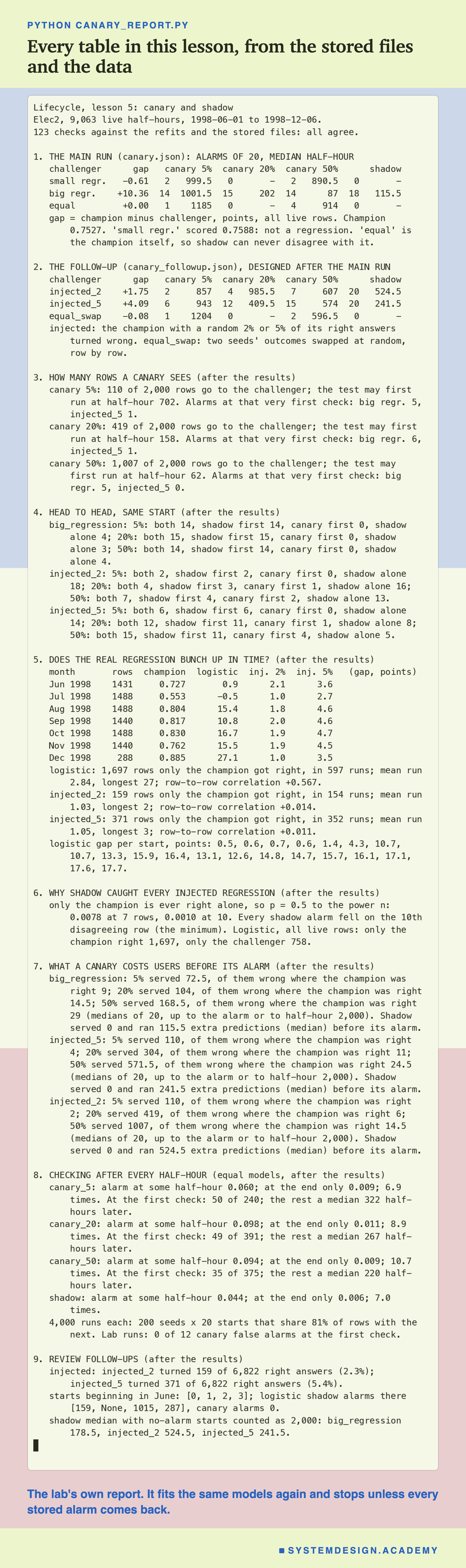
The report lives in scripts/labs/lifecycle/canary_report.py. It reads the lab's stored files, results/canary.json and results/canary_followup.json, lesson 1's stored file, and the Elec2 data from scikit-learn's local copy. The lab stored the half-hour of each first alarm, not each model's right and wrong rows, so the report trains the lab's four models again with the same data, split and settings, rebuilds the follow-up's challengers with its own seeds, and replays every rule on every start. It stops unless every stored first alarm, count, median and gap comes back exactly. It makes 123 checks in all, and they all agree. It changes nothing in the lab's files.

Its json mode writes every number to results/cn-report.json, which the figures read. The demo mode checks the student script's stored run, and the box mode writes the playground below and checks that it gives the lab's alarms.

This box has no model in it. It holds the real right-or-wrong outcome of four models on all 9,063 live rows: the champion, the logistic model, and the follow-up's two injected challengers, one hexadecimal digit per row (counting in sixteens, with the digits 0 to 9 and a to f). It also holds the lab's own random canary draws. The report checked that every canary and shadow alarm it gives matches the lab's stored files. It runs in your browser.

As it is, the box prints the four rows of the lab for the 4.09-point regression: 6, 12, 15 and 20 alarms of 20, with the lab's medians. Try table('logistic', CHAMP, LOGISTIC) for the main run's big regression, and table('2%', CHAMP, INJ2) for the smaller one.

Then look for false alarms: table('the same model', CHAMP, CHAMP) gives the canary's false alarms on the champion against itself. Change the random draw with canary(CHAMP, CHAMP, 0, my_assign(50, 7)), and try a few seeds; None means no alarm in 2,000 half-hours. Every start in STARTS is a half-hour of the live period where the lab began watching.

Loading. fetch_openml("electricity", version=1) downloads Elec2 once and reads the local copy after that. The label column holds the words UP and DOWN, turned into 1 and 0. cut is 36,249: the champion learns from the rows before it, and the 9,063 rows after it are the live traffic.

The champion. One boosted-trees model with seed 0. champion is a list of True and False, one per live row: right or wrong. This list is all either rollout needs.

The challenger. spoil gives each live row a 5% chance of being marked, with the follow-up's own seed, 4. champion & ~spoil keeps the champion's result everywhere except on the marked rows, where a right answer becomes wrong and a wrong one stays wrong. The draw turned 371 of the champion's 6,822 right answers, 5.4%, which is why the challenger is worse by 4.09 points, and it is never right where the champion is wrong.

The canary draw. to_new marks the rows that go to the challenger: a random 20% of the first 2,000, with the lab's seed, 0.

canary. Walks through the half-hours in order. Each row adds to the counts of the model that answered it. Once both models have at least 30 rows, it computes the pooled error rate (pool, the share of all rows so far answered wrong), the typical wobble se, and the z value, and returns the first half-hour where z is above 2.33.

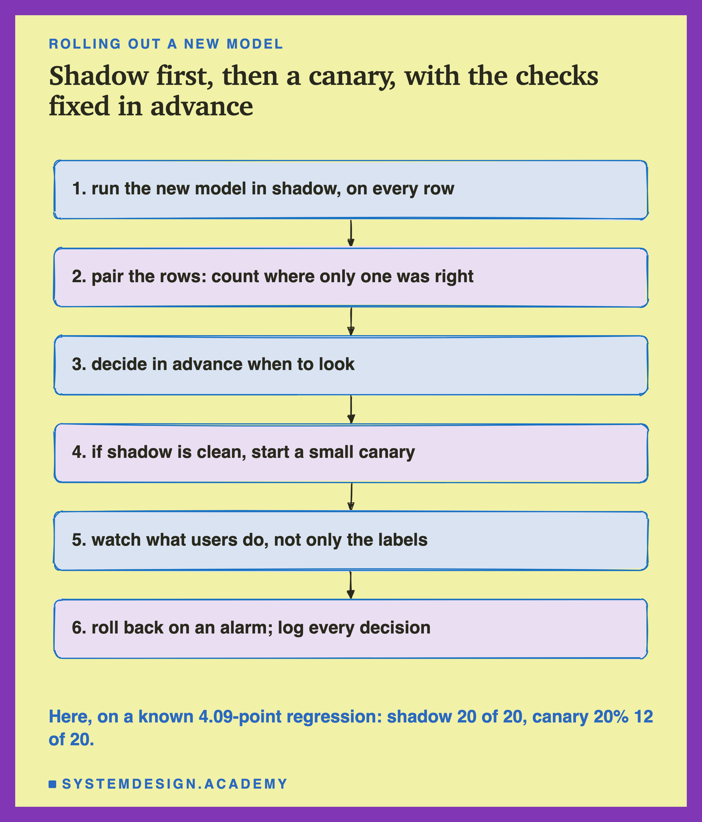
Run the new model in shadow first. Send every live row, or a large sample of rows, to both models. Show users only the champion's answer, and store the challenger's answer with the row.

Pair the rows. When each label arrives, mark both models right or wrong on that row. Count the rows where only the champion was right and the rows where only the challenger was right, and test that split with McNemar's test, as in lesson 4.

Decide in advance when to look. Choose the checkpoints before the rollout starts, for example once a day, and test only there, or use a method designed for repeated looks. Write the checkpoints, the bar and the minimum number of rows into the rollout's configuration.

If shadow is clean, start a small canary. Send a small share of real traffic to the challenger. Work out first how many labelled rows that share will give per day, and how long it will need to see the size of problem you care about.

Watch what users do. In the canary, measure the things shadow cannot see: clicks, returns, complaints, payments. Accuracy on labels is only part of the picture.

Roll back on an alarm, and log every decision. Keep the champion ready to take all traffic back at once: that is the roll back. Record each check, its counts and its result.

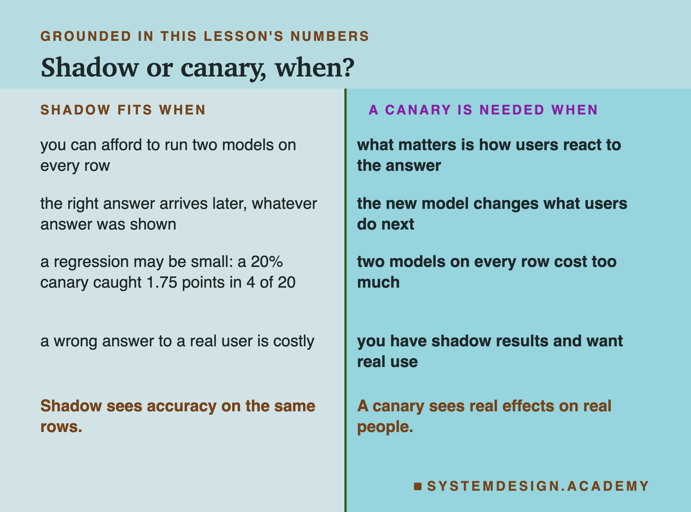
Use shadow when you can afford two models on every row. For small models, the extra compute is cheap. For large ones, shadow a sample of the traffic rather than none of it.

Use shadow when the right answer arrives later and does not depend on which answer was shown. Here the price goes up or down whatever the model says, so every row gets a label for both models, and that is what makes shadow possible to score. In many products the label exists only for the answer users saw: whether someone clicked a recommendation can only be known for the recommendation they were shown. There shadow cannot measure accuracy at all. And when a label takes weeks, every alarm waits for it, in shadow and canary alike.

Use shadow when the regression you fear is small. Here a 20% canary caught a 1.75-point regression in only 4 of 20 starts, where shadow caught it in all 20. The injected errors are the easiest case for shadow, as the earlier slide showed; the canary's count is affected much less by how the errors were made.

Use shadow when a wrong answer to a real user is costly. Shadow shows no one the new answers.

Use a canary when what matters is how users react. Shadow never shows its answers, so it can never see a click, a purchase or a complaint.

Use a canary when the model changes what users do next. If the answer changes the next request, the rows shadow sees are not the rows the new model would really meet.

Do not use a small canary to look for a small regression. Here a 5% canary answered 110 rows in almost 42 days.

Do not check a canary after every batch with a fixed bar. Here that raised the false alarms from about 1% to 6 to 10%.

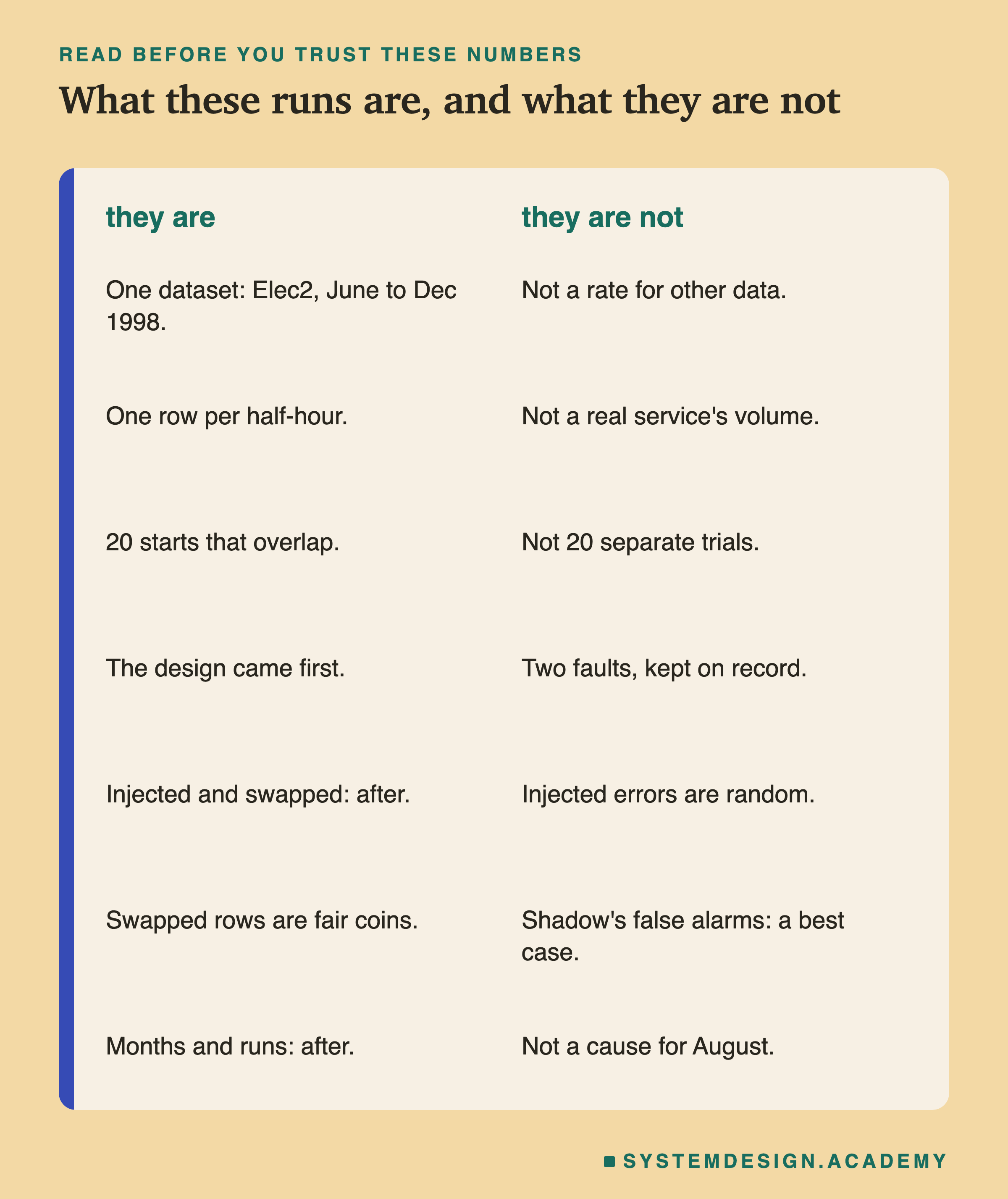
One dataset, one champion. Everything here is boosted trees on Elec2, June to December 1998. The results depend on how often the two models disagree and on how the data changes over the months. With other data they would move.

One row per half-hour. A real service may have far more labelled rows per hour. Read every time in this lesson as a number of rows, not as a time a real service would take.

Twenty starts that overlap. Each start watches 2,000 half-hours, and neighbouring starts are about 372 half-hours apart, so they share about 81% of their rows. The lab also used the same canary draw at every start. The counts out of 20 are counts, not 20 separate trials, and I did not test them.

Two faults, kept on the record. The planned small regression was 0.61 points better, and the planned equal challenger could not test shadow. The follow-up replaced them, and it was designed after the main results and written down before it ran.

Injected errors are random, and so are the swaps. They suit a paired test that treats rows as coin flips, and they never point the other way, which is the easiest case for shadow. The swapped equal pair likewise makes every disagreeing row a fair, separate coin, so shadow's 0 of 20 and 4.4% false alarms are a best case too. The real regression came in runs and in seasons. This lab did not measure how much that changes shadow's speed or false alarms.

After the results. The first allowed check, the head-to-head, the per-start and per-month gaps, the runs, the tenth-row alarm, the rows served and the repeated-checking rates were all measured after I saw the results. Why the logistic model fell behind from August is a guess, not a measurement.

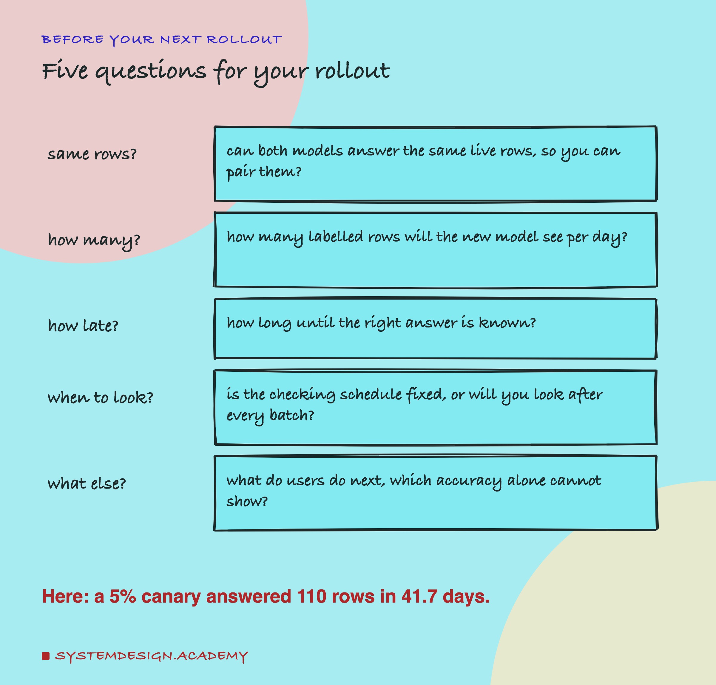
Find how your team rolls out a new model, and ask the five questions on the card. If the answer to "same rows?" is yes and you are not running shadow, you are not using the fastest check this lab found. If the answer to "when to look?" is "whenever someone opens the dashboard", your false alarms are several times higher than the bar you think you set.

Then run a small version of this lab on your own traffic. Take your current model's stored right-and-wrong results on recent rows, make a known regression by turning a few percent of its right answers wrong, and measure how many rows your canary and your shadow check need to see it. Then do the same with a real older model in place of the injected one, since a real regression may not be as tidy.

The chapter plan's next lesson asks when to retrain: on a schedule or when something triggers it, and what each costs, on the same time-ordered data.