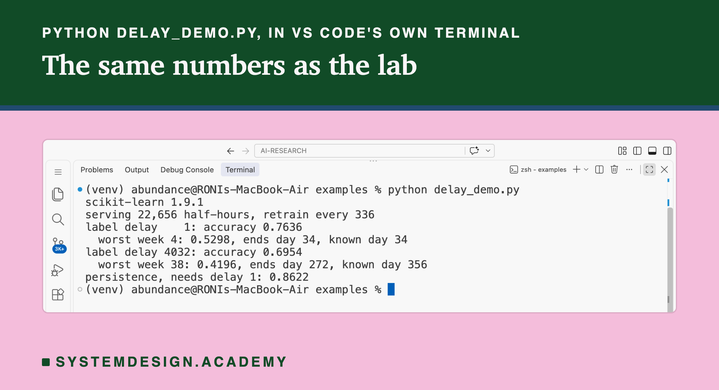
The Marks That Came Back Late
Imagine a teacher who gives his class a short test every Friday. On Monday he gets the marks back, sees which topics the class got wrong, and teaches those again that week. It works well. The class drifts off course for a few days at most before he notices and steers it back.
Now imagine the tests have to be sent away to be marked, and the marks come back three months later. Every week he still teaches, and every week the class still takes a test. But the marks he reads this Monday are from a test the class took in the spring. He is correcting mistakes his students made long ago, some of which they have already grown out of, and he has no idea at all how last Friday went.

Two things got worse for him at once. The first is learning: his lesson plans are built on old evidence, so they fit the class of three months ago, not the class in front of him. The second is knowing: if the class is struggling right now, he will not find out for three months. Both are the same problem seen from two sides. The answers that tell him how he is doing arrive late.
This lesson is about the same problem in a program that learns from examples. I kept one model, retrained it every week exactly as in lesson 6, and made its right answers arrive later and later. Then I measured what it cost the model, and what it cost the people watching it.
Where This Lesson Starts
This chapter follows one model through its life, on the same electricity data. When to retrain compared retraining on a schedule with retraining on a trigger, and found that retraining every week kept the model at 0.7636 where a model that was never retrained, with every label fresh at launch, fell to 0.6610. The promotion gate and canary and shadow measured how a team judges a model with live answers. Stale pieces in a pipeline looked at checks that need no answers at all, and lineage and rollback at getting an old model back.
Every one of those lessons quietly assumed something about this data: that the right answer for a half-hour arrives half an hour later. Lesson 6 said so on its last results slide, gave the headline numbers of this lesson's lab as a preview, and promised to come back to it. This is that lesson. I will not re-teach how the weekly schedule works or why a model goes stale; lesson 6 did both.
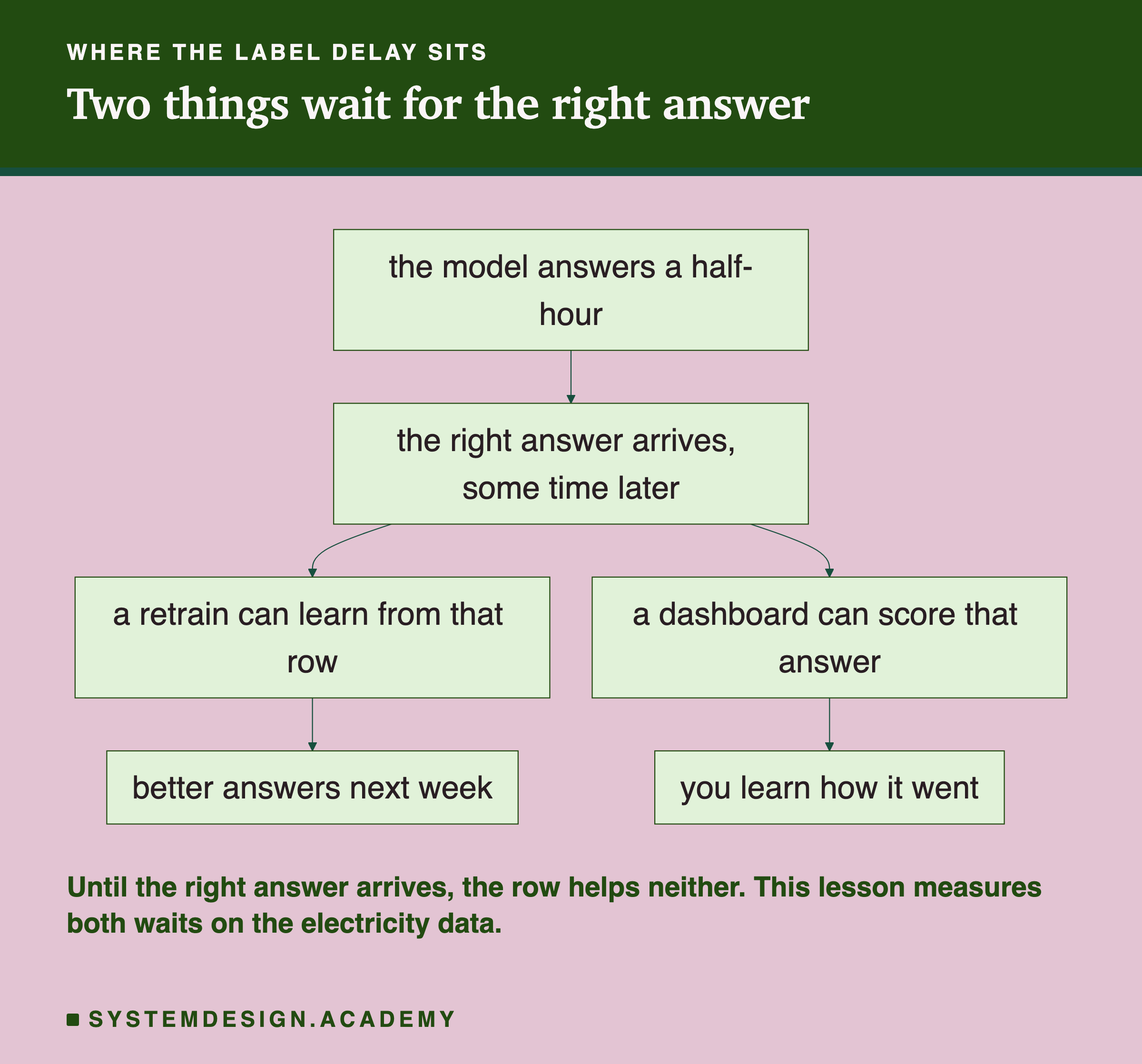
The flowchart shows why a late answer matters twice. When the right answer for a row arrives, two things can happen. A retrain can learn from it, and a dashboard can score the model on it. Until it arrives, it does neither. So a label delay slows down learning and slows down knowing, and this lesson measures both.
Ten Words for This Lesson
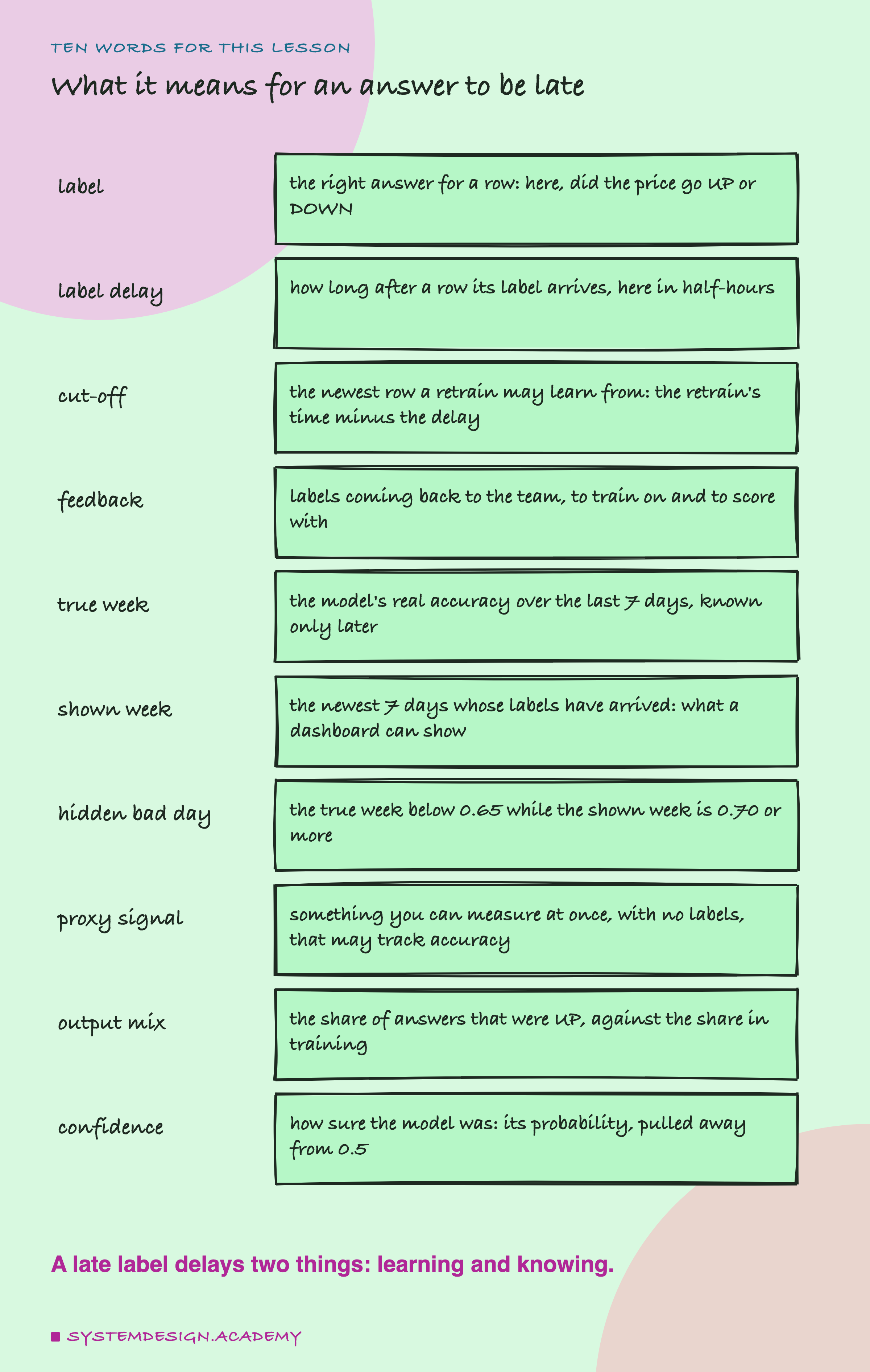
A label is the right answer for a row: here, whether the electricity price went UP or DOWN against its average over the last 24 hours. Accuracy is the share of rows a model got right, and a point is one hundredth of accuracy.
The label delay is how long after a row its label arrives. In this lesson I count it in half-hours, because that is how the data is stored: a delay of 48 is one day, 336 is one week. Because of the delay, a retrain can only learn from rows whose labels have already arrived. The newest row it can use is its cut-off: the time of the retrain minus the delay. Feedback is the general word for labels coming back to the team, both to train on and to score the model with.
Three words are about watching the model. The true week is the model's real accuracy over the last 7 days. Nobody can see it at the time, because its labels have not arrived. The shown week is what a dashboard can show instead: the accuracy over the newest 7 days whose labels have arrived. I call a day a hidden bad day when the true week was below 0.65 while the shown week was 0.70 or more, so the dashboard said "fine" while the model was doing badly.
The last three words are about what a team can watch without labels. A signal is a measurement you can make at once, with no right answers, in the hope that it moves with accuracy. The output mix is one: the share of the model's answers that were UP, compared with the share of UP in the labels it was trained on. Lesson 7 used it. is another: how sure the model was, measured by how far its probability of UP sat from 0.5.
Where Answers Come Back Late
The electricity data is unusually kind. Whether the price went up or down is known as soon as the next price is in. Most real systems are not like that, and it helps to see a few before looking at numbers.
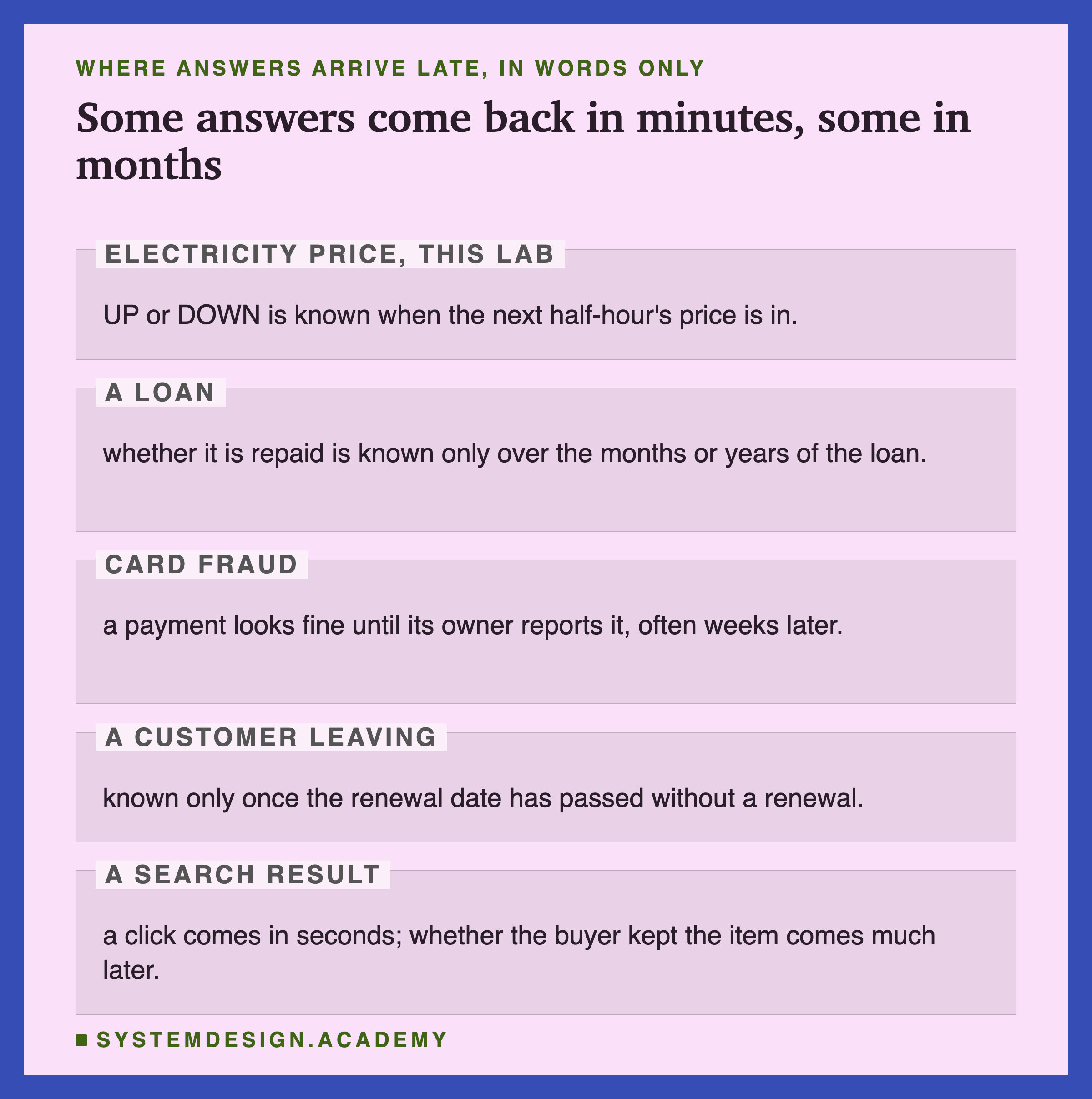
A loan. A bank's model decides whether to lend. Whether that was a good decision is known only as the borrower pays, or fails to pay, over months or years. A model retrained this month learns from loans that were made long ago, in a different economy.
Card fraud. A payment is approved in a fraction of a second. If it was fraud, the true owner often notices it on a statement and disputes it, which can take weeks. Until then the payment sits in the data looking like an honest one.
A customer leaving. A company predicts which customers will not renew. It learns the truth only after each renewal date passes, which can be a month or a year away.
A search or shop result. A click arrives in seconds, which is why many systems train on clicks. Whether the buyer kept the item, or regretted it, comes much later. A team that wants the slower, truer label has to wait for it.
I give no numbers for these, because I have not measured any of them. They are here to show that the delays in this lab, up to twelve weeks, are not extreme. They are ordinary.
What a Retrain Can Learn From
Before running anything, it is worth seeing exactly what a delay takes away from a retrain. The sketch shows the first weekly retrain of the served half, at row 22,992, for three delays, with the rows drawn to scale.
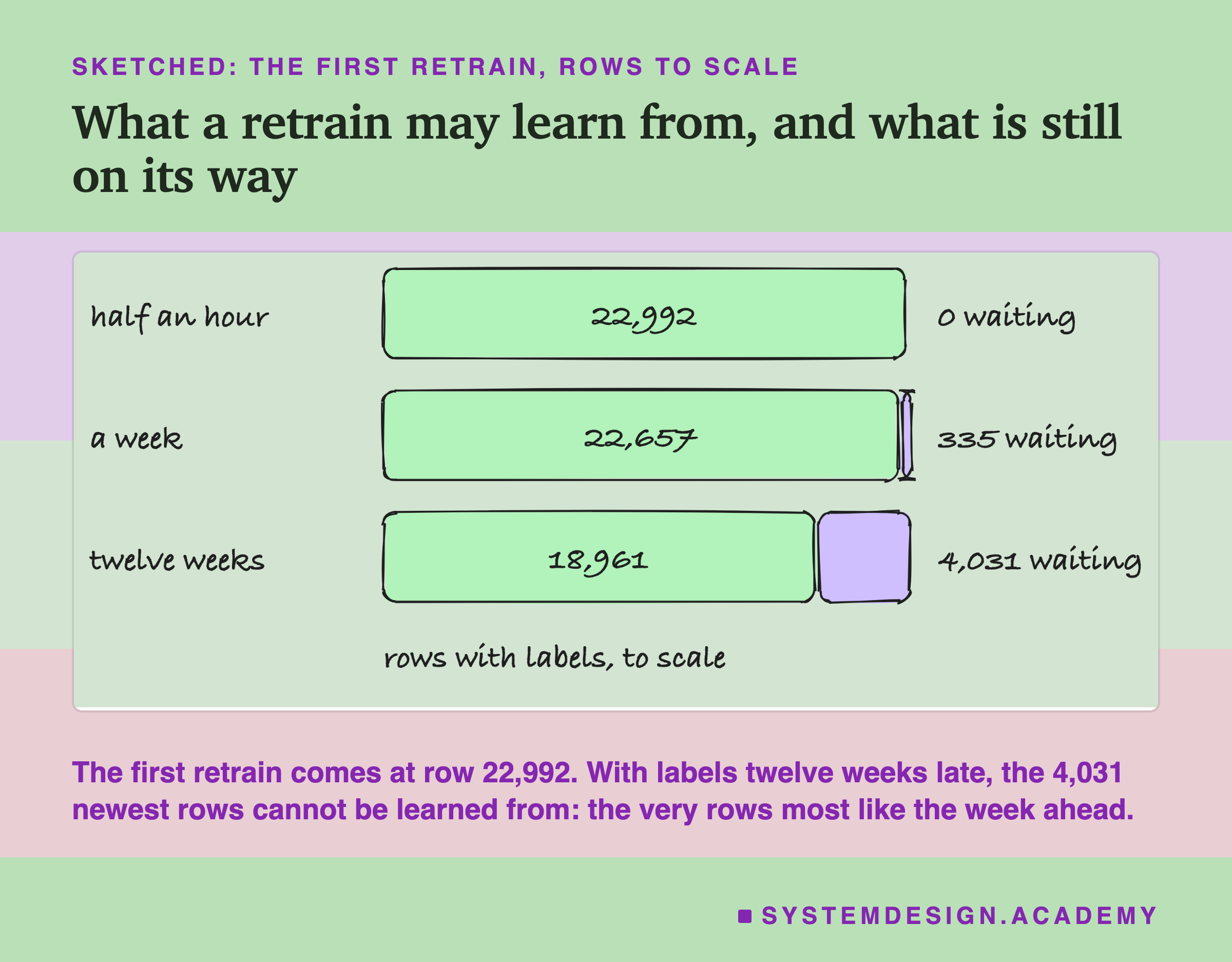
With a delay of half an hour, the retrain learns from every row before it. With a delay of a week, the newest 335 rows, a week less one half-hour, are still waiting for their labels. With a delay of twelve weeks, 4,031 rows are waiting. Those are not random rows. They are the newest ones, the rows most like the week the new model is about to serve.
This is the whole mechanism of the cost. A late label does not make the data wrong or make training worse at its job. It pushes the cut-off back, so every retrain produces a model that is a little older on the day it starts work. A model trained with twelve weeks of labels missing is, in effect, a model trained twelve weeks earlier and put into service twelve weeks late.
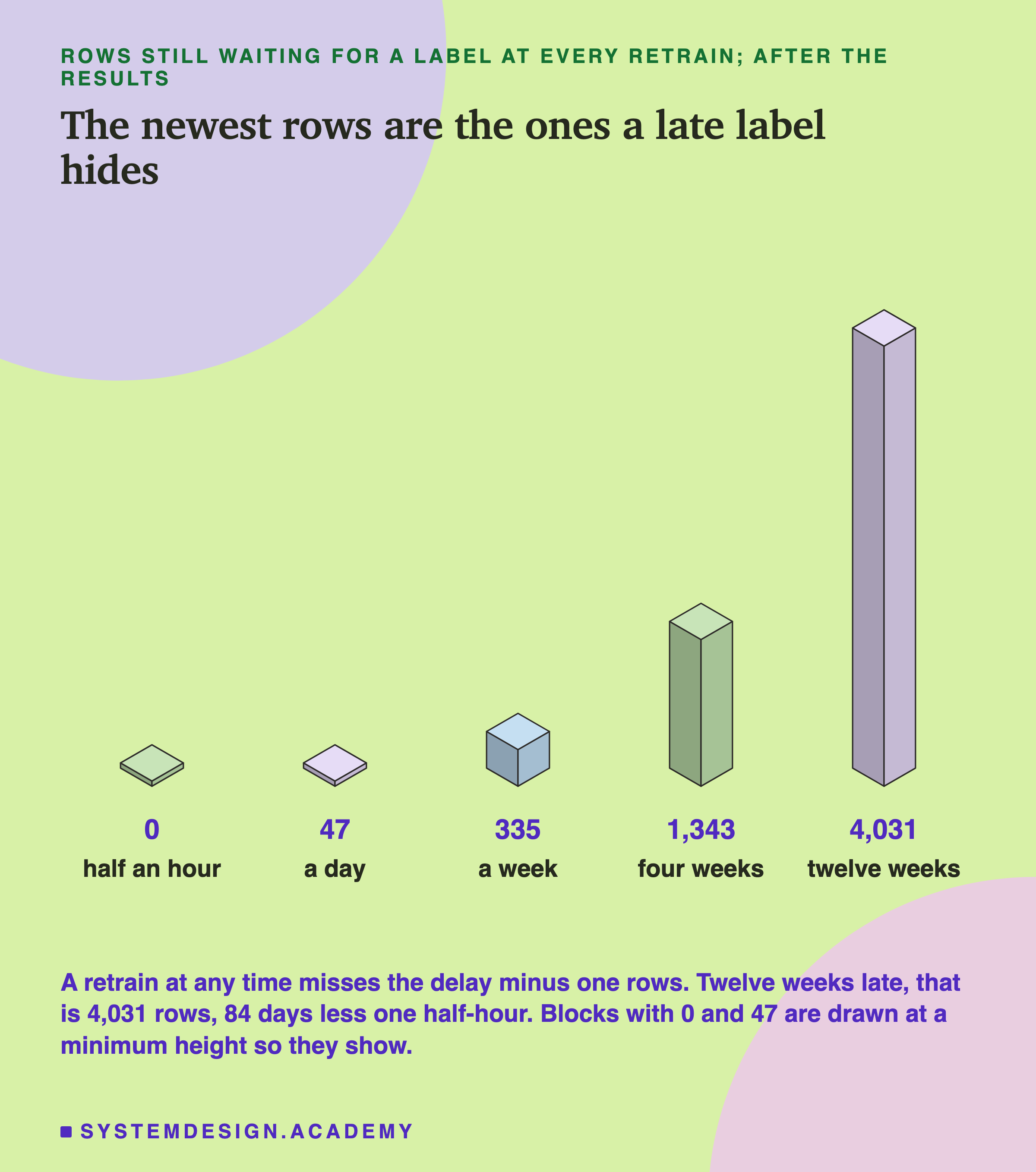
I worked out the numbers on this drawing after the results, but they need no lab at all: at any retrain, the rows still waiting are the delay minus one. That is 0, 47, 335, 1,343 and 4,031 rows for the five delays, or up to 84 days of data. The question the lab answers is what those missing rows are worth.
The Lab: Five Waits, One Schedule
I wrote the lab's design at the top of its file, delay_lab.py, before it ran. The dated entry is in the chapter plan (2026-09-29, "DELAY LAB (batch 9) designed before running").
The data is Elec2 again: 45,312 half-hours of the New South Wales electricity market, in time order. The model is the boosted trees of the earlier lessons, many small trees of yes-or-no questions built one after another, with early stopping switched off and seed 0, so that training twice on the same rows gives the same model (lesson 2 measured why). It is the exact weekly policy of lesson 6: first trained on the first half of the rows, then it serves the second half, 22,656 half-hours from 22 August 1997 to 6 December 1998, one day at a time, and it is retrained every 336 half-hours on every row up to its cut-off.
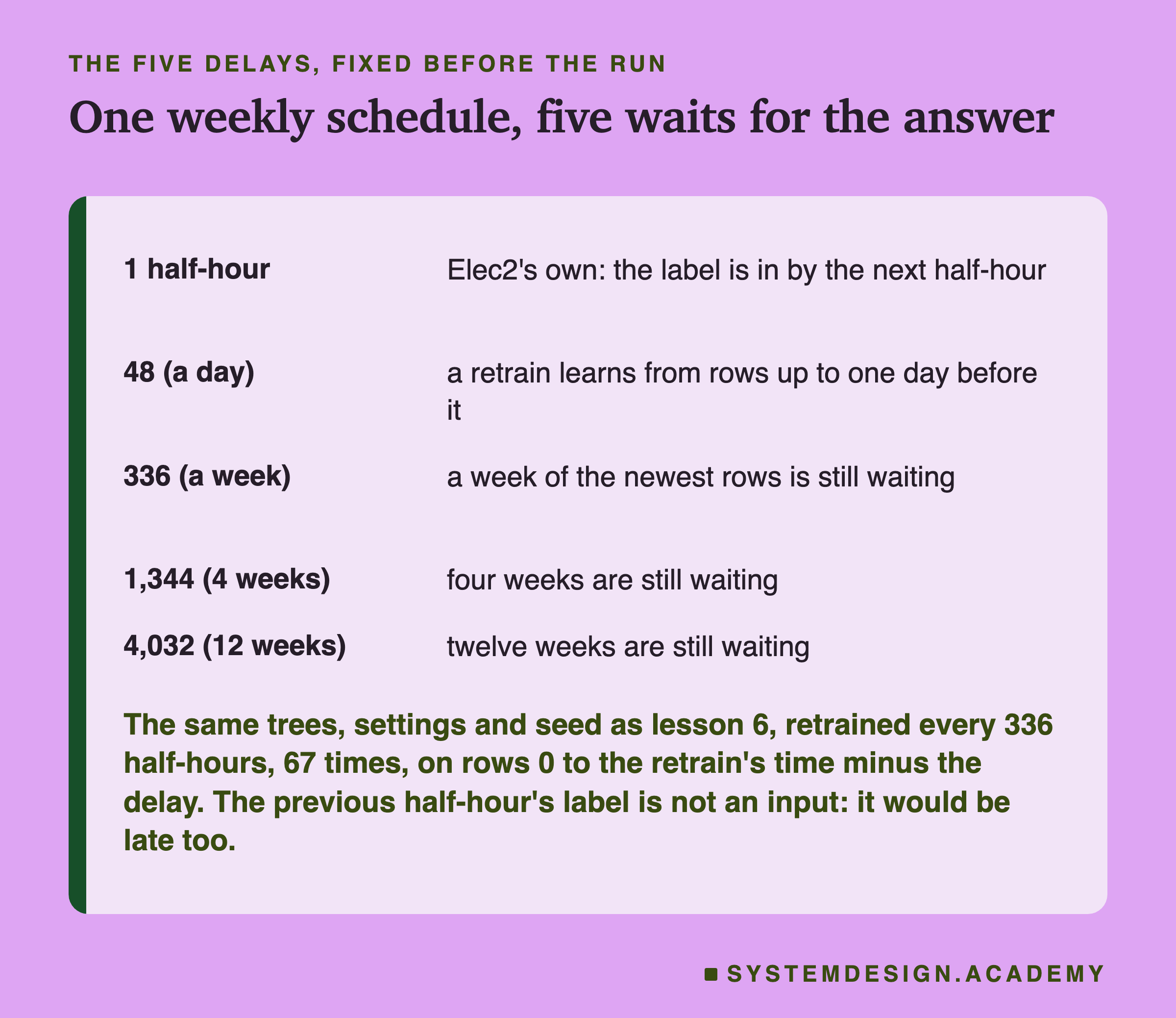
The five delays were fixed in the design: 1 half-hour (Elec2's own), 48 (a day), 336 (a week), 1,344 (four weeks) and 4,032 (twelve weeks). Every delay got the same 67 retrains at the same moments; only the cut-off moved.
One input was deliberately left out. Lesson 1 found that the previous half-hour's label is a very strong input on this data. With late labels, that input would be late too, so the design did not use it. Persistence, the rule that simply repeats the previous half-hour's label, is reported only for the delay of half an hour, because at any longer delay it cannot be computed.
The design asked for the accuracy over the served half for each delay, per 28-day block, and "the monitoring view": what a team could have known about the model on each day. One run per delay. The design described the numbers and declared no significance test, a calculation of how likely a difference is to come from chance alone.
What Each Wait Cost
Here is what the lab stored in results/delay.json.
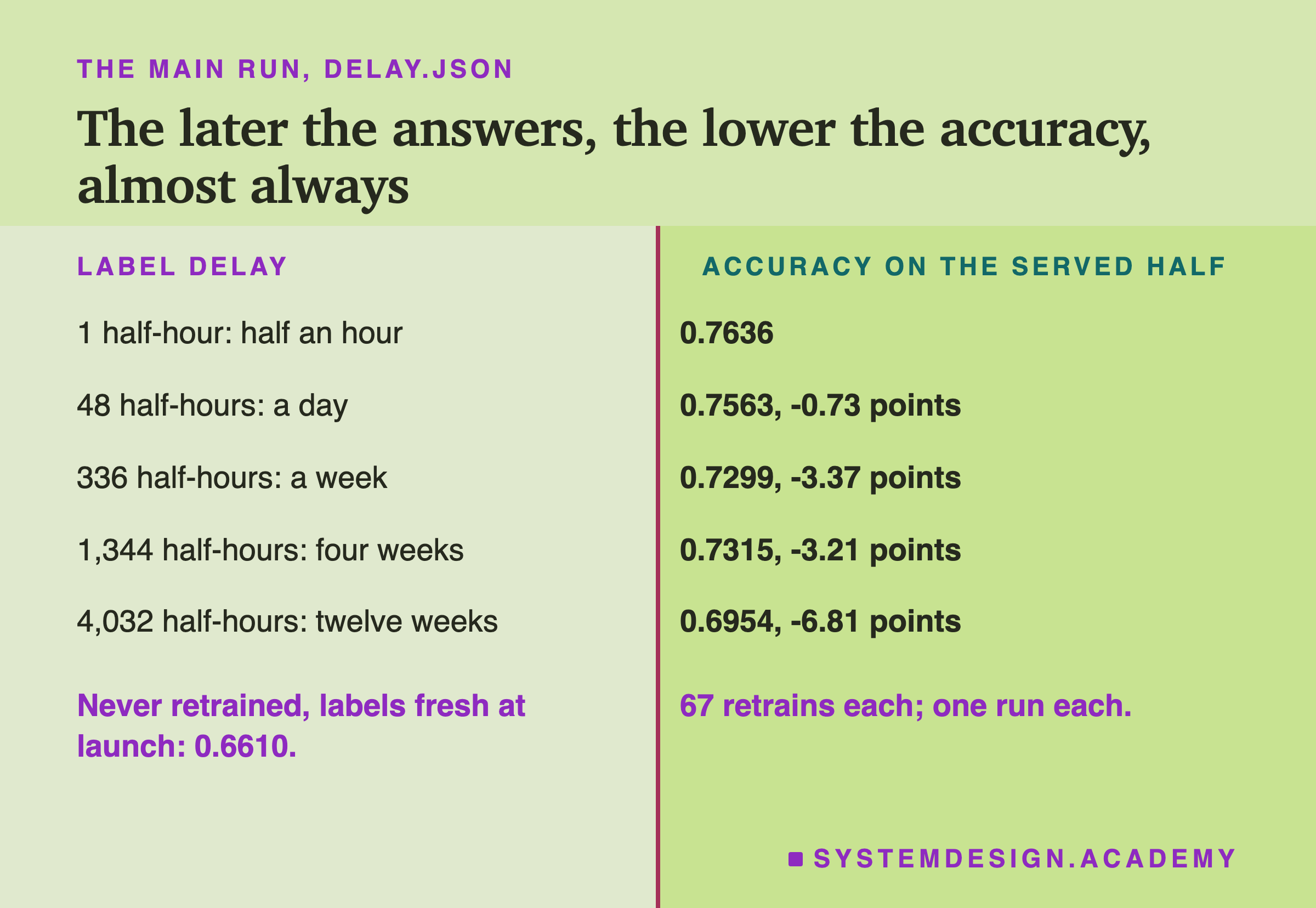
First, a cross-check. With labels half an hour late, the lab scored 0.7636, exactly the weekly result of lesson 6, and every one of its 17 block scores matched. So this lab and lesson 6's are the same machine, and the only thing changing below is the delay.
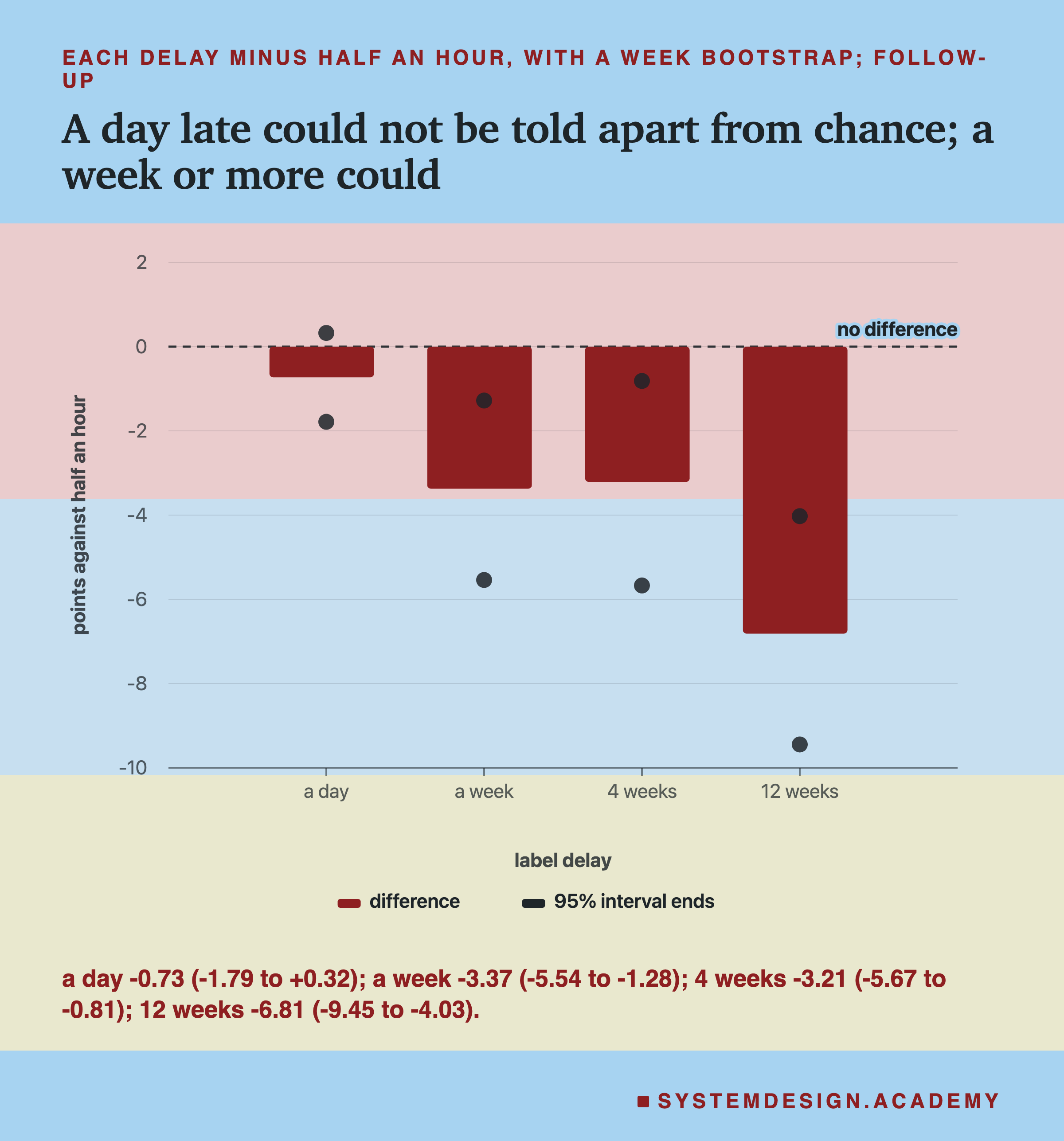
A delay of a day cost 0.73 points. A week cost 3.37 points: 764 fewer half-hours right out of 22,656. Four weeks cost 3.21 points, slightly less than a week. Twelve weeks cost 6.81 points, bringing the model to 0.6954.
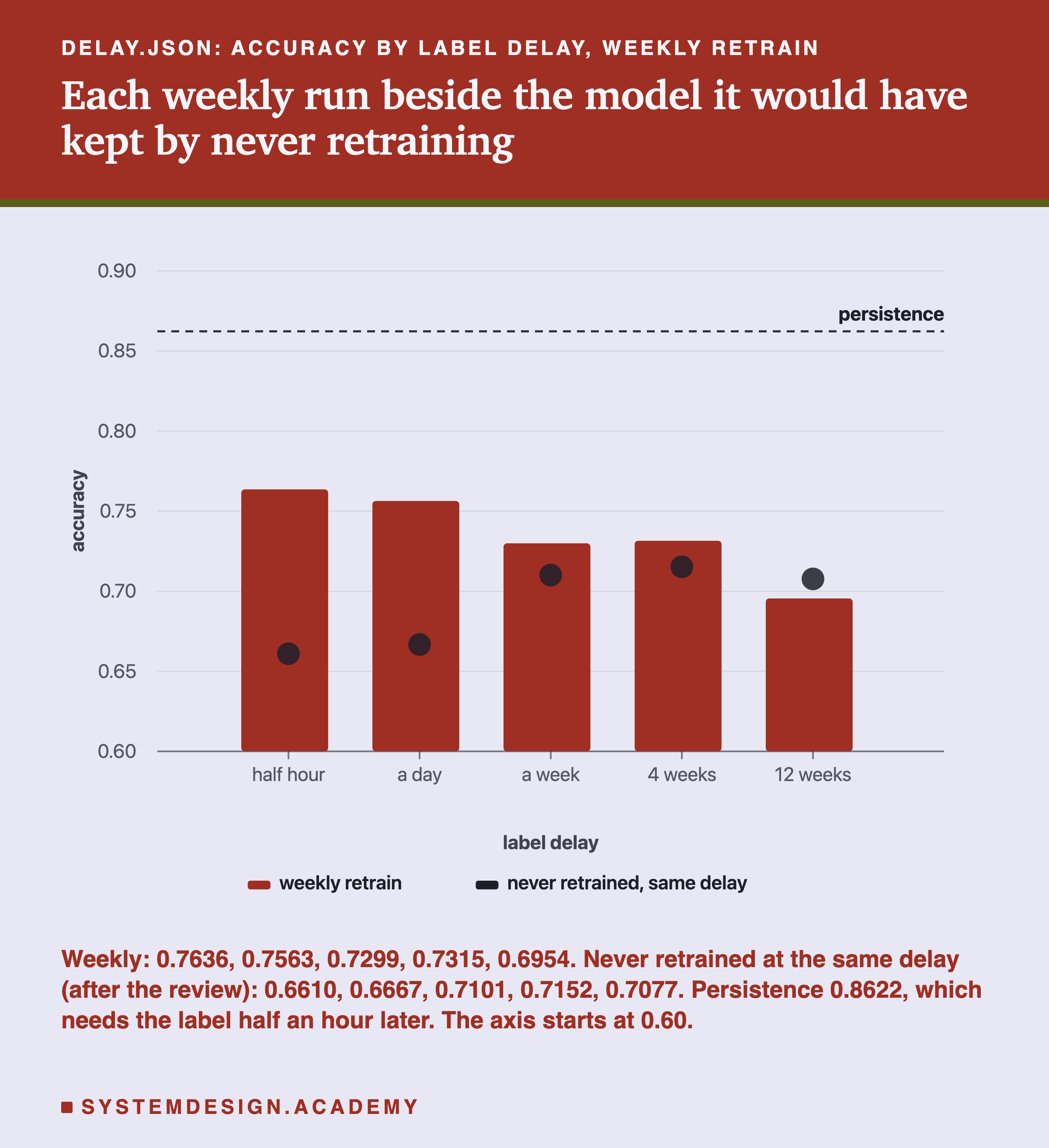
Two things on this chart matter. The first is the dots. Each one is the model the same team would have had if it had never retrained at all: its own first model, trained on the rows whose labels had arrived on launch day, and kept for the whole served half. I added these dots after a review of this lesson, and a later slide explains why. Half an hour late and a day late, retraining every week scored far above its dot. A week and four weeks late, only a little above. Twelve weeks late, it scored below its dot: 0.6954 against 0.7077. So the easy lesson, that old labels are always better than no new labels, did not hold here at twelve weeks.
The second is the top line. Persistence, the rule that learns nothing, scored 0.8622, higher than any trained model in this lab. But it needs the label from half an hour ago. With any delay longer than that, it does not exist. On this data, the best answer of lesson 1 is only available because the labels come back so fast, which is a reason to value a fast label beyond what it does for training.
Month by Month
One number over 472 days hides when the delay mattered. Here is each 28-day block for three of the delays.
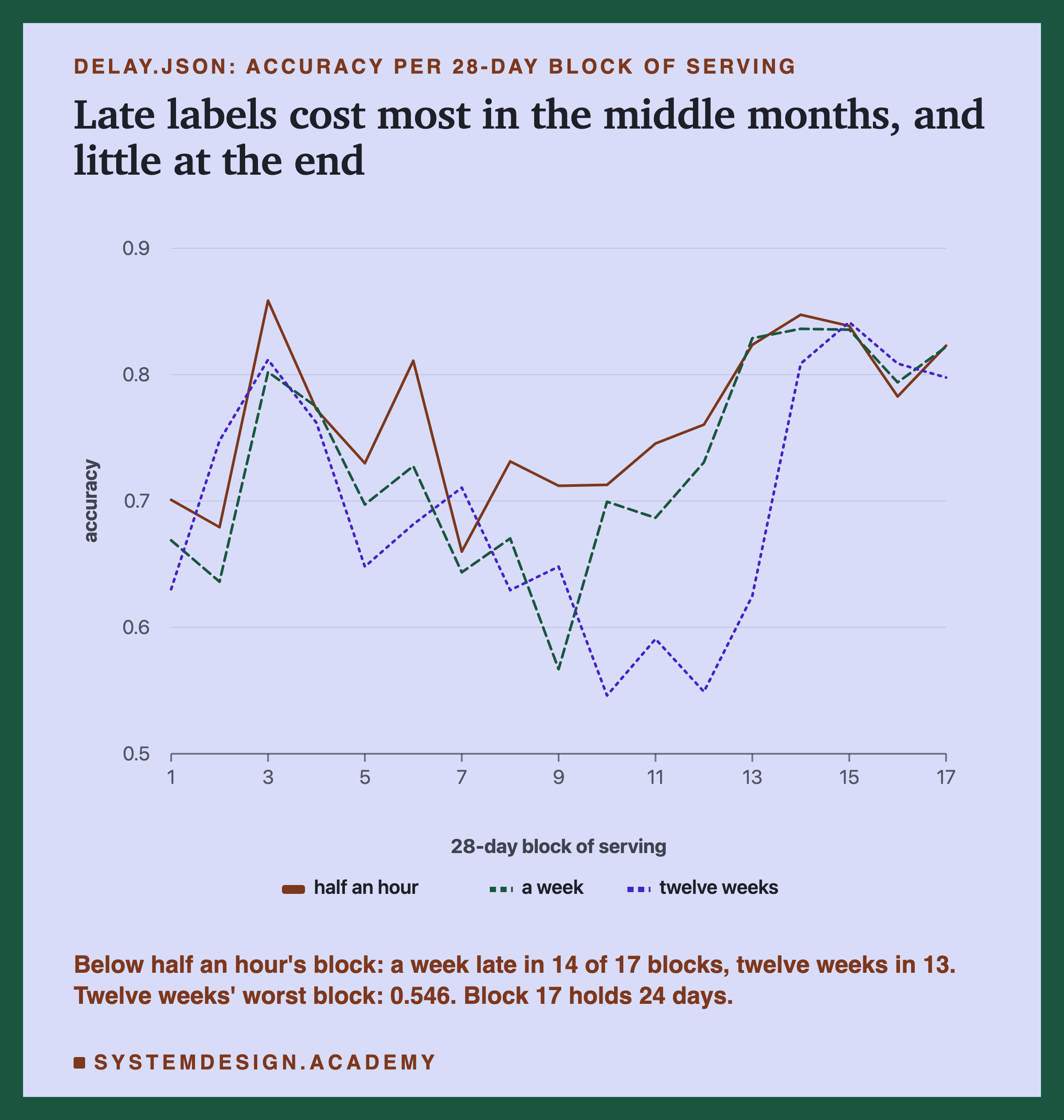
A delay did not cost the same everywhere. A week late was below the half-hour run in 14 of the 17 blocks and above it in 3. Twelve weeks late was below in 13 and above in 4. A day late was below in 11 and above in 6, which is closer to a coin than a steady cost.
The largest losses came in the middle of the run. Twelve weeks late, the worst block was block 10, at 0.5461, where the half-hour run scored 0.7128. A week late, the worst was block 9, at 0.5670. In the last four blocks all five delays came back together, between 0.7418 and 0.8527. I worked out the block counts after the results.
A possible reason, and it is a guess: a delay costs most when the market is changing, because that is when the missing newest weeks carry information the older rows do not. When the market is steady, the older rows teach the same lesson, and the delay costs little. I did not measure how fast the market changed in each block, so this stays a guess.
Did Four Weeks Really Beat One Week?
The main result had one odd point: four weeks late scored 0.7315 and one week late 0.7299. If a later label always costs more, that is backwards. So after seeing the results I designed a follow-up to ask whether the difference was real. I wrote its design into the lab file's followup mode before it ran, and its results are in results/delay_followup.json.
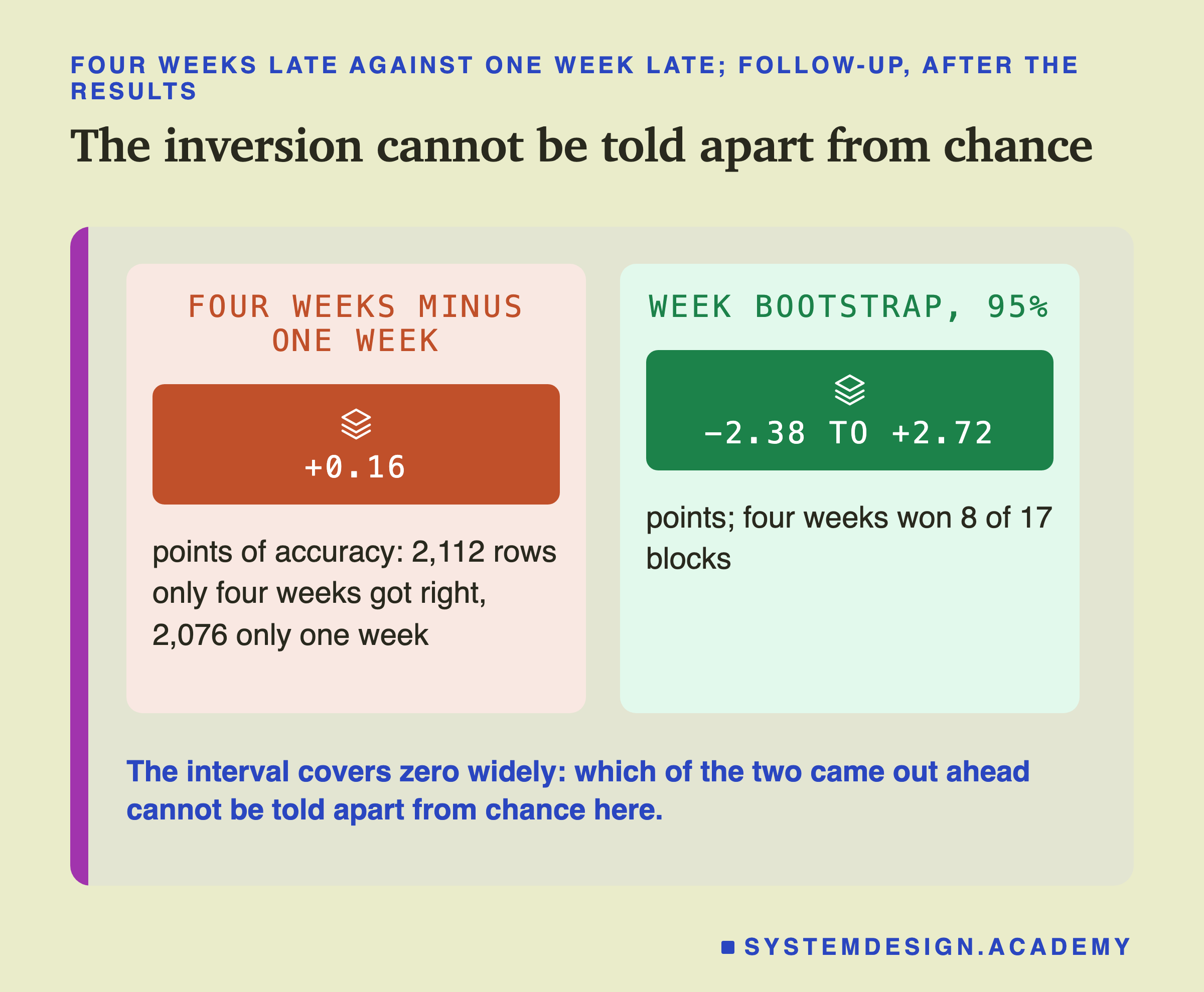
The two runs were scored on the same 22,656 rows, so I compared them row by row. On 2,112 rows only the four-week model was right, and on 2,076 only the one-week model was. On all the other rows they agreed. A difference of 36 rows out of 22,656 is the whole of the inversion.
The follow-up used two ways to judge it. McNemar's test looks only at those disagreeing rows and asks how surprising a split of 2,112 against 2,076 would be if the two models were equally good. Its answer is the p-value of lesson 4: how often a split at least this uneven would happen by chance alone if the two models were equally good. Here p = 0.59, so more than half the time: nothing surprising. But McNemar's test assumes every row is independent, and neighbouring half-hours are not: prices move in runs, so errors come in runs too. That makes its p too small here, not too large, so it is only a first look.
The fairer check is a bootstrap: build 2,000 new versions of the served period by drawing whole weeks at random, with replacement (a week drawn once can be drawn again, so some weeks appear twice and some not at all), and measure the difference on each. Keeping weeks whole keeps the runs of errors together. The middle 95% of those differences ran from −2.38 to +2.72 points. The interval covers zero widely. Four weeks won 8 of the 17 blocks. Which of the two came out ahead cannot be told apart from chance here.
What the Dashboard Could Show
Now the second half of the problem: knowing. The design promised "the monitoring view", and the main run did not store it, so I added it to the follow-up. For every served day, at the end of the day, it computed two numbers: the true week, the real accuracy over the last 7 days, and the shown week, the accuracy over the newest 7 days whose labels had arrived. The shown week is the best any dashboard could honestly draw.
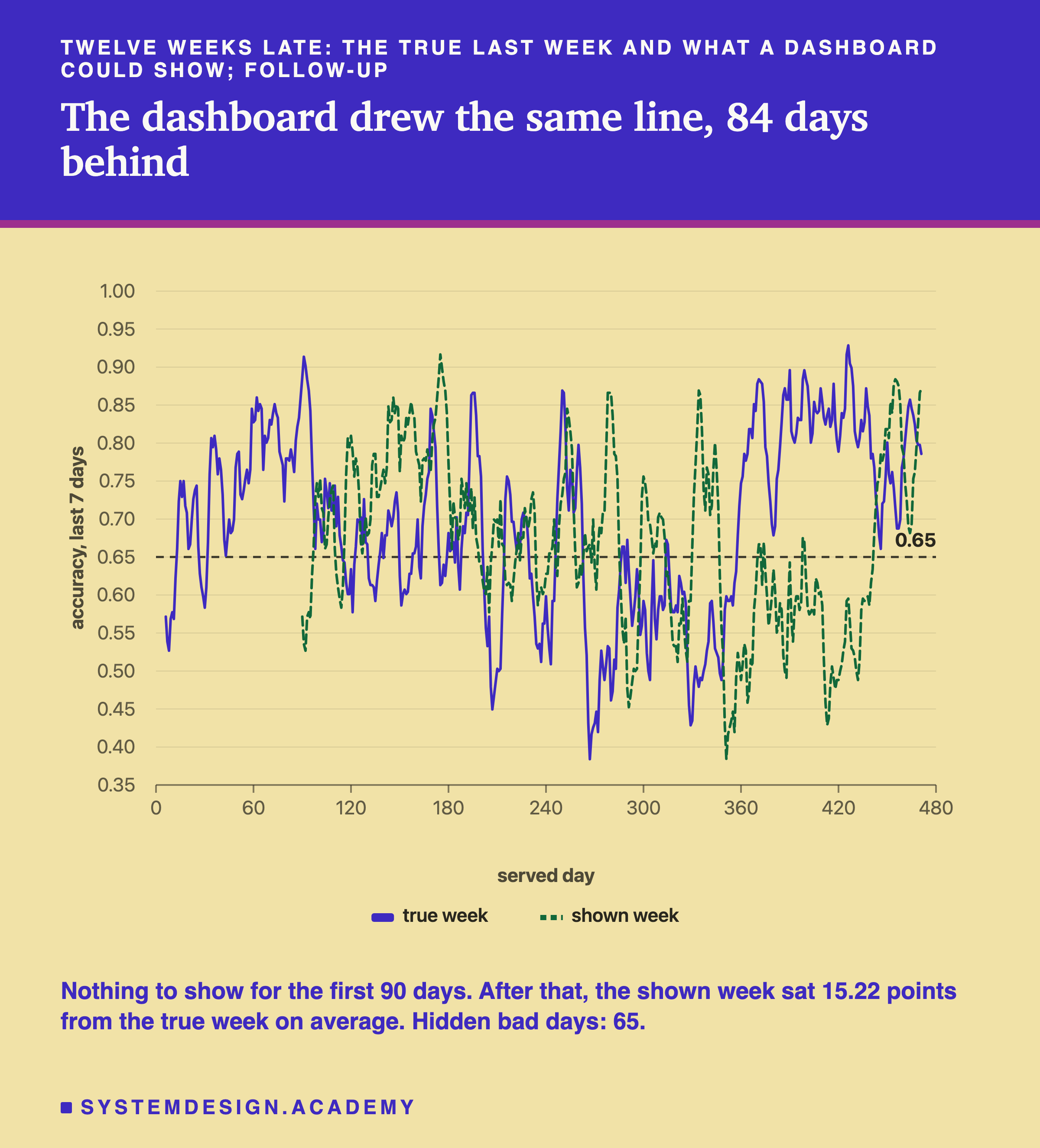
With labels twelve weeks late, the dashboard had nothing at all to show for the first 90 days of serving: no week with all its labels in yet. After that, it drew the same line as the truth, 84 days behind. On average, over the 382 days where both existed, the shown week sat 15.22 points away from the true week. A week late the gap was 8.48 points, four weeks late 9.54, and a day late 2.67.
That gap is not an error in the dashboard. Every number it shows is exactly right about the week it describes. The problem is which week that is. A number that is correct about a week 84 days ago, placed under a heading like "accuracy, last 7 days", tells a reader something false about now.
A delay also changes what the first days look like. Half an hour late, the dashboard shows nothing for the first 6 days, until it has its first full week. Twelve weeks late, it shows nothing for the first 90. A newly launched model with late labels flies blind for longer than the delay itself.
Bad Weeks That Looked Fine
A gap of 15 points on average is abstract. The follow-up also counted the days when the gap would have misled someone. The two levels, 0.65 and 0.70, are round numbers I took from lesson 6's follow-up, and I had already seen those results when I chose them.
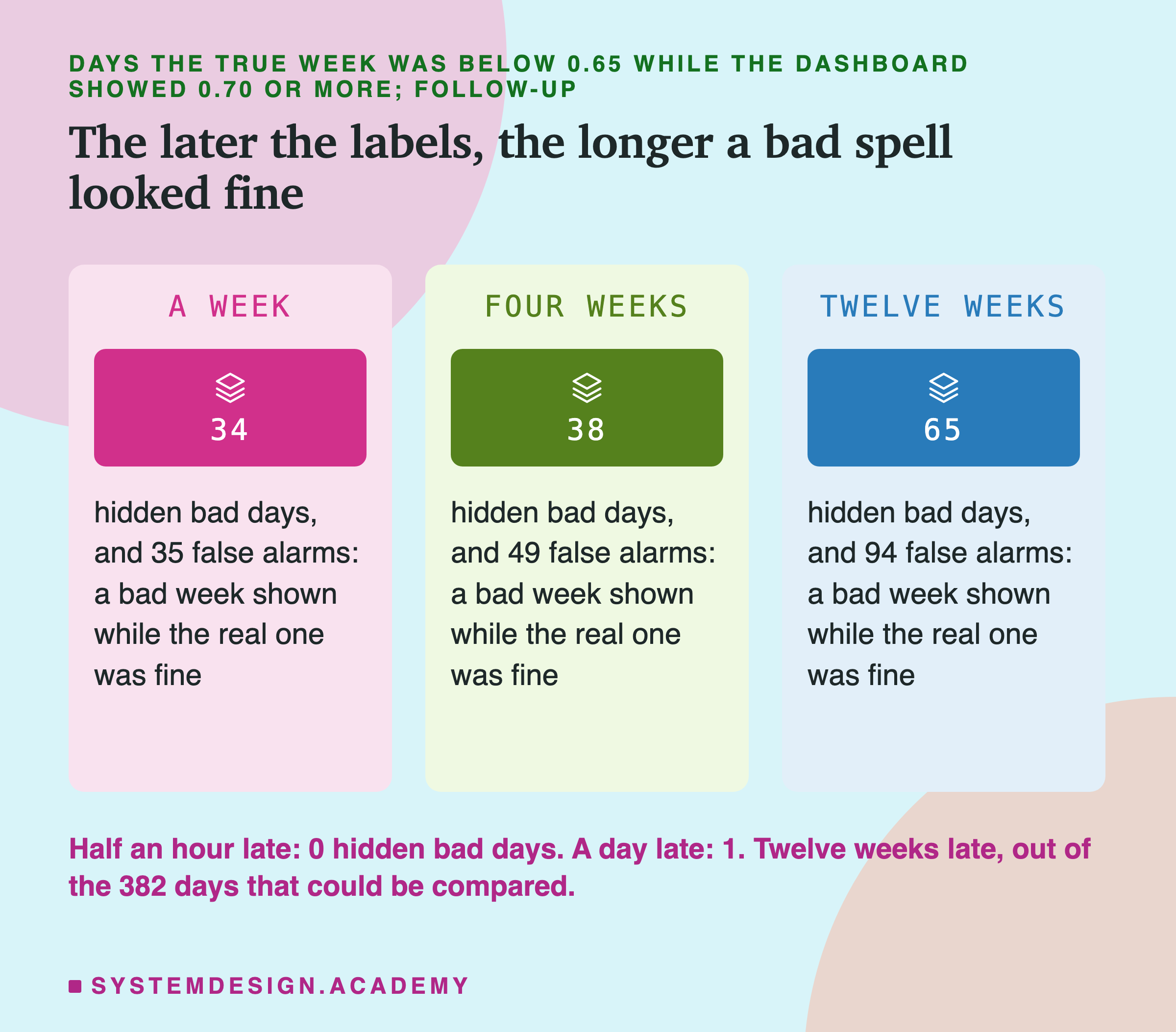
A hidden bad day is a day when the true week was below 0.65 while the shown week was 0.70 or above. Half an hour late there were none, by definition. A day late, 1. A week late, 34. Four weeks late, 38. Twelve weeks late, 65 of the 382 days that could be compared. On each of those days, anyone looking at the chart would have seen a model doing fine, while it was doing badly.
The reverse happened too. A false alarm day is a day when the true week was 0.70 or more while the shown week was below 0.65: the chart said the model was in trouble when it was not. There were 4 a day late, 35 a week late, 49 four weeks late, and 94 twelve weeks late. A team that reacts to the chart, say by rolling back or retraining, would have reacted to the wrong weeks both ways.
I also measured how long each bad spell took to show. A bad spell is a run of days where the true week stayed below 0.65. Twelve weeks late there were 16. The first began on the seventh served day and showed on the chart exactly 84 days later. But the longest, 42 days from 4 July to 14 August 1998, showed on the chart the day it began. That was not knowledge. The shown week on that day was about a week 84 days earlier, which happened to be bad too. When two bad periods are 84 days apart, the late chart looks right by coincidence. So a count of "days until shown" can flatter a late dashboard, and I do not use it as a headline.
One Bad Week, Twelve Weeks Late
Here is one real week, the worst week of the twelve-week run, followed from the day it happened to the day anyone could know. I picked it after the results, as the week with the lowest accuracy.
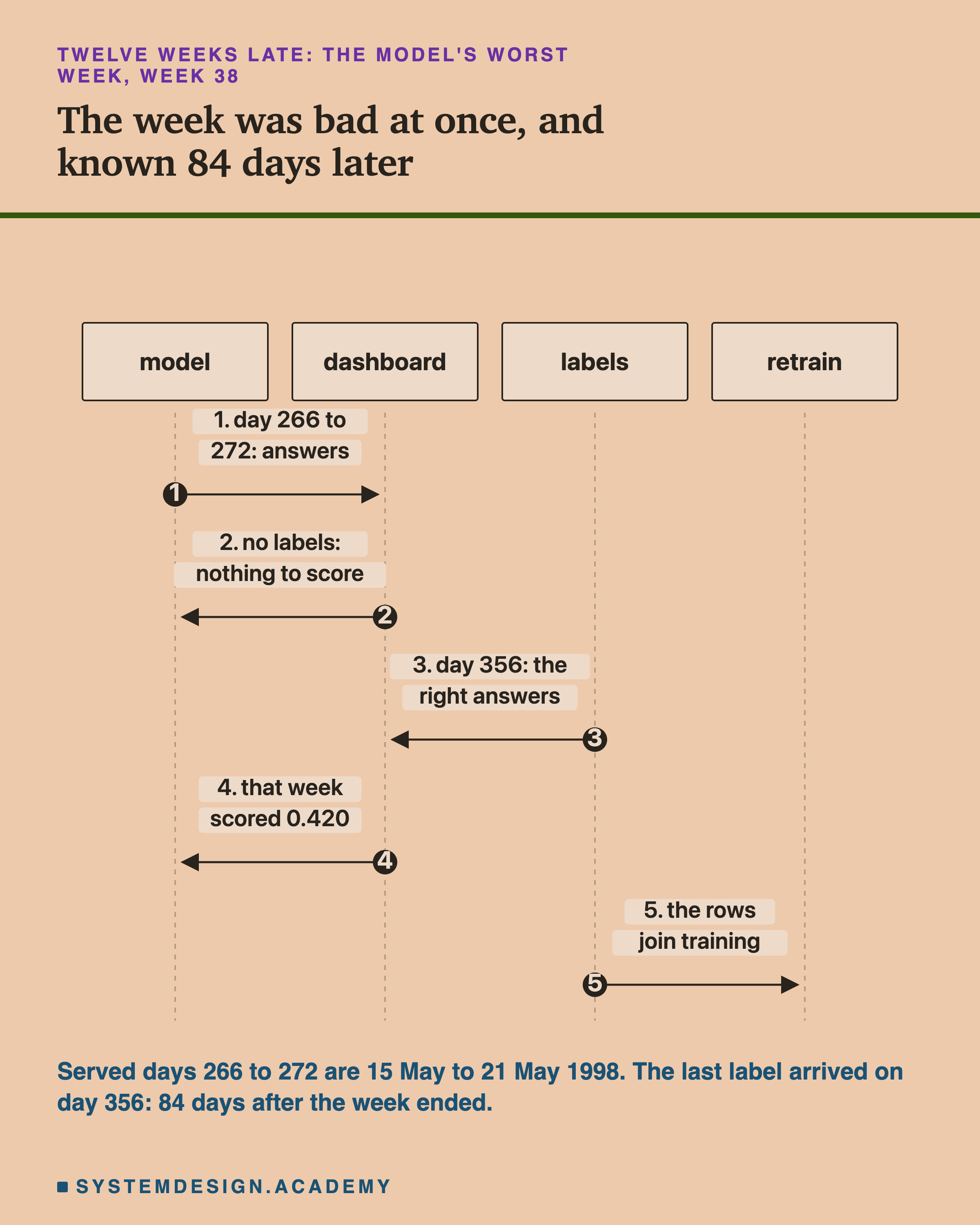
In served week 38, 15 to 21 May 1998, the model retrained with twelve-week-old labels got 0.4196 of its answers right: worse than tossing a coin. During that week, the dashboard had its answers but no labels, so there was nothing to score. The last label of the week arrived on served day 356, 84 days after the week ended. Only then could anyone compute the 0.4196. On the same day, those rows became available to the next retrain.
So the model made its worst mistakes in May, and the earliest moment a team could have seen them, and the earliest moment the model could have learned from them, was mid-August. Everything that happened in between was decided without that information.
The half-hour run's worst week was a different one: week 4, 19 to 25 September 1997, at 0.5298. Its marks were in the same day. A late label does not only make the bad weeks worse. It moves them, because the model that serves each week is a different, older model.
The Date Input, Again
Lesson 6 had a surprise: most of what retraining bought on this data came from repairing one input, the date. A model trained once sees dates only up to the end of its training, and as the served dates run past that, its trees keep answering as if it were still the last training day. Retraining moves the training dates forward and repairs that. I wondered whether the date also explained part of the delay's cost, so the follow-up ran all five delays again with the date input set to 0 on every row, as lesson 6's follow-up did.
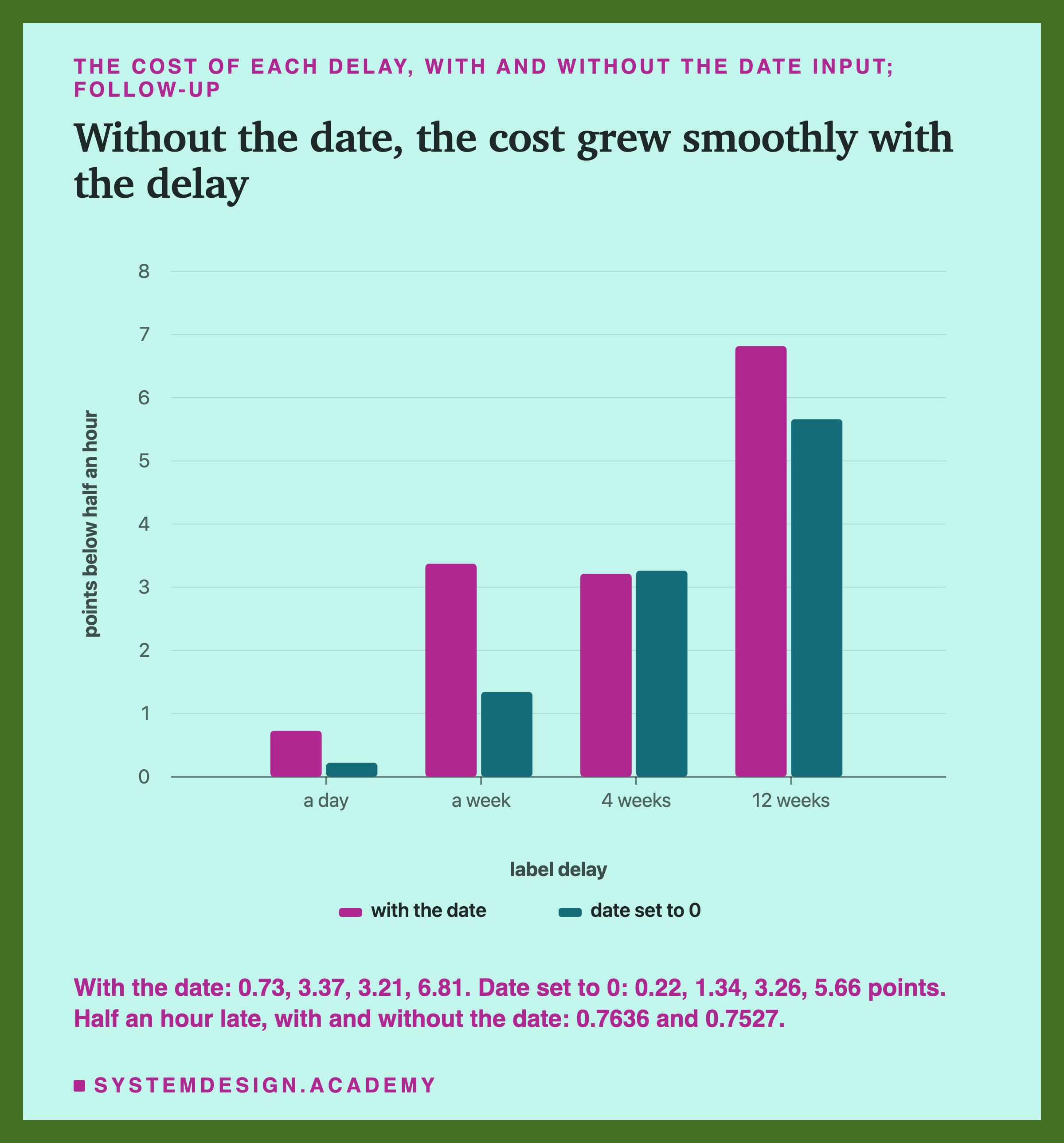
Without the date, half an hour late scored 0.7527, exactly lesson 6's weekly run without the date, which is the follow-up's own cross-check. Then the cost grew smoothly with the delay: 0.22 points for a day, 1.34 for a week, 3.26 for four weeks, 5.66 for twelve weeks. The inversion between a week and four weeks disappeared.
One thing follows, and I measured it after the results: the date helped most when the labels were fresh. Half an hour late, the model with the date scored 1.09 points above the one without. Twelve weeks late, the date made no difference at all: 0.6954 with it, 0.6962 without. One possible reason: the date lets a model separate the newest months from the older ones, and when the newest months are missing, there is nothing new for it to separate.
In my first draft, this slide went on to say that the date input decides whether late retraining beats never retraining. That was wrong, and the next slide shows the real reason: I had been comparing with the wrong "never".
A Fair Never
My first draft compared every delay with one line: lesson 6's model that was never retrained, at 0.6610. On that comparison, even twelve weeks late, weekly retraining won by 3.45 points, and I wrote that old labels were still better than no new labels. A review of the draft found the flaw. Lesson 6's frozen model learned from every row before serving began, with every label already in. A team whose labels arrive twelve weeks late could never have built it: on launch day, its newest 4,031 rows had no labels yet. I now call that line "never retrained, labels fresh at launch".
The fair "never" for each delay is the model that same team would really have had: its own first model, trained on the rows whose labels had arrived, and kept for the whole served half. I wrote this check into the lab file, as its fairnever mode, after the review and before it ran, with and without the date input. Its results are in results/delay_fairnever.json. At the half-hour delay it gives exactly lesson 6's 0.6610 and, without the date, lesson 6's 0.7208, which is its own cross-check.
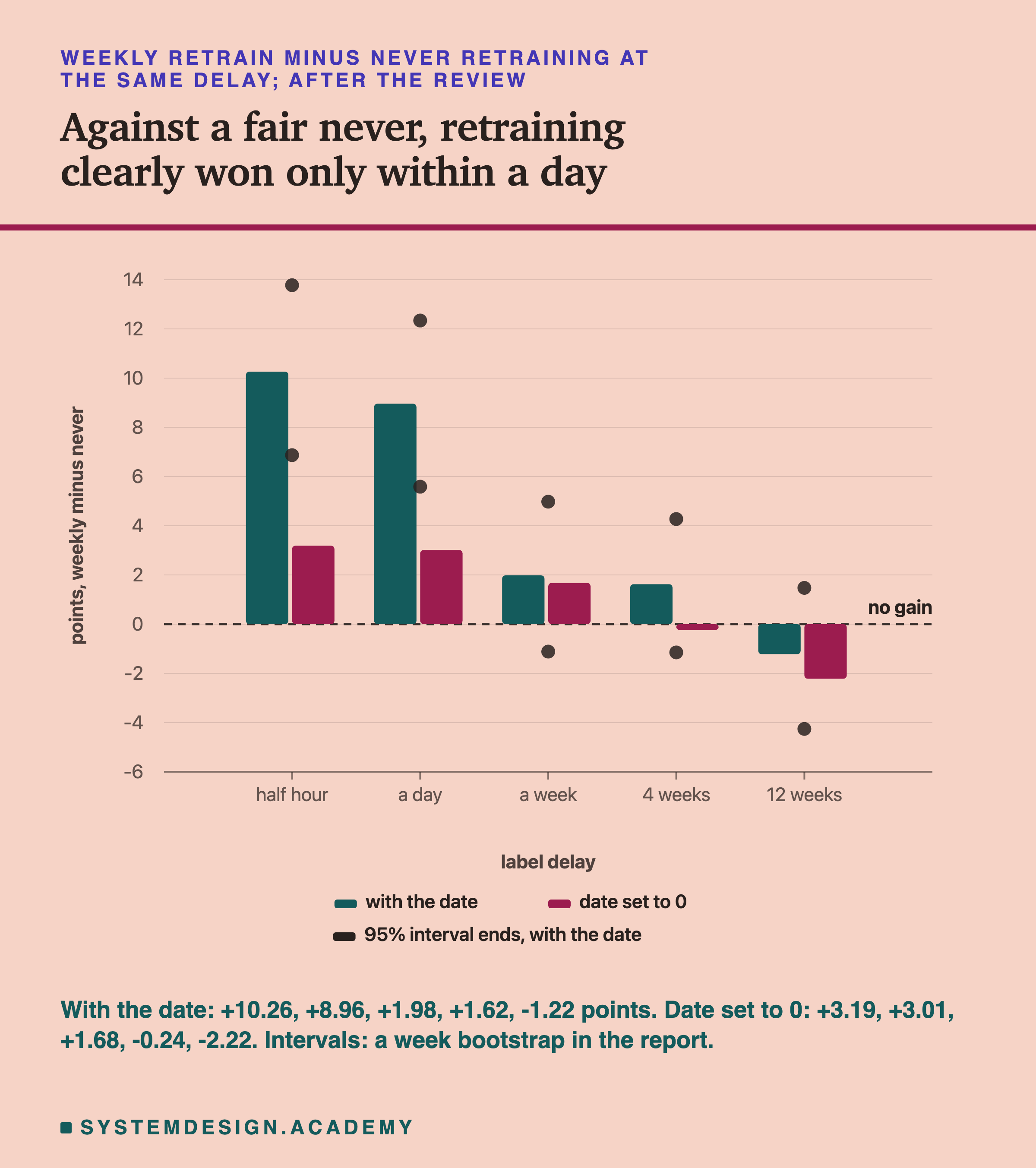
With the date, the fair never scored 0.6610, 0.6667, 0.7101, 0.7152 and 0.7077 for the five delays. Weekly retraining minus never was +10.26 points half an hour late and +8.96 a day late. The report then ran the same week bootstrap as before on these pairs, which I added after the review: those two intervals, 6.87 to 13.78 and 5.59 to 12.34, sit far above zero. A week late the gain was +1.98 (−1.12 to +4.98), four weeks late +1.62 (−1.15 to +4.28): both cannot be told apart from chance. Twelve weeks late it was −1.22 (−4.26 to +1.47): retraining scored lower than never retraining, though that too cannot be told apart from chance.
Without the date the pattern is the same, a little sharper: +3.19 and +3.01 points half an hour and a day late, +1.68 a week late, −0.24 four weeks late, and −2.22 twelve weeks late, with an interval of −4.01 to −0.35, entirely below zero. So the date input is not what decides this. The unfair baseline was. With a fair never, retraining every week on labels a day old clearly helped here, and retraining on labels twelve weeks old did not help, with the date or without it.
What You Can Watch While You Wait
While the labels are on their way, a team is not completely blind. It can see the model's answers the moment they are given, and the model's own probabilities. The follow-up tested two signals built from those, for each of the 67 full served weeks: the output mix, and the confidence.
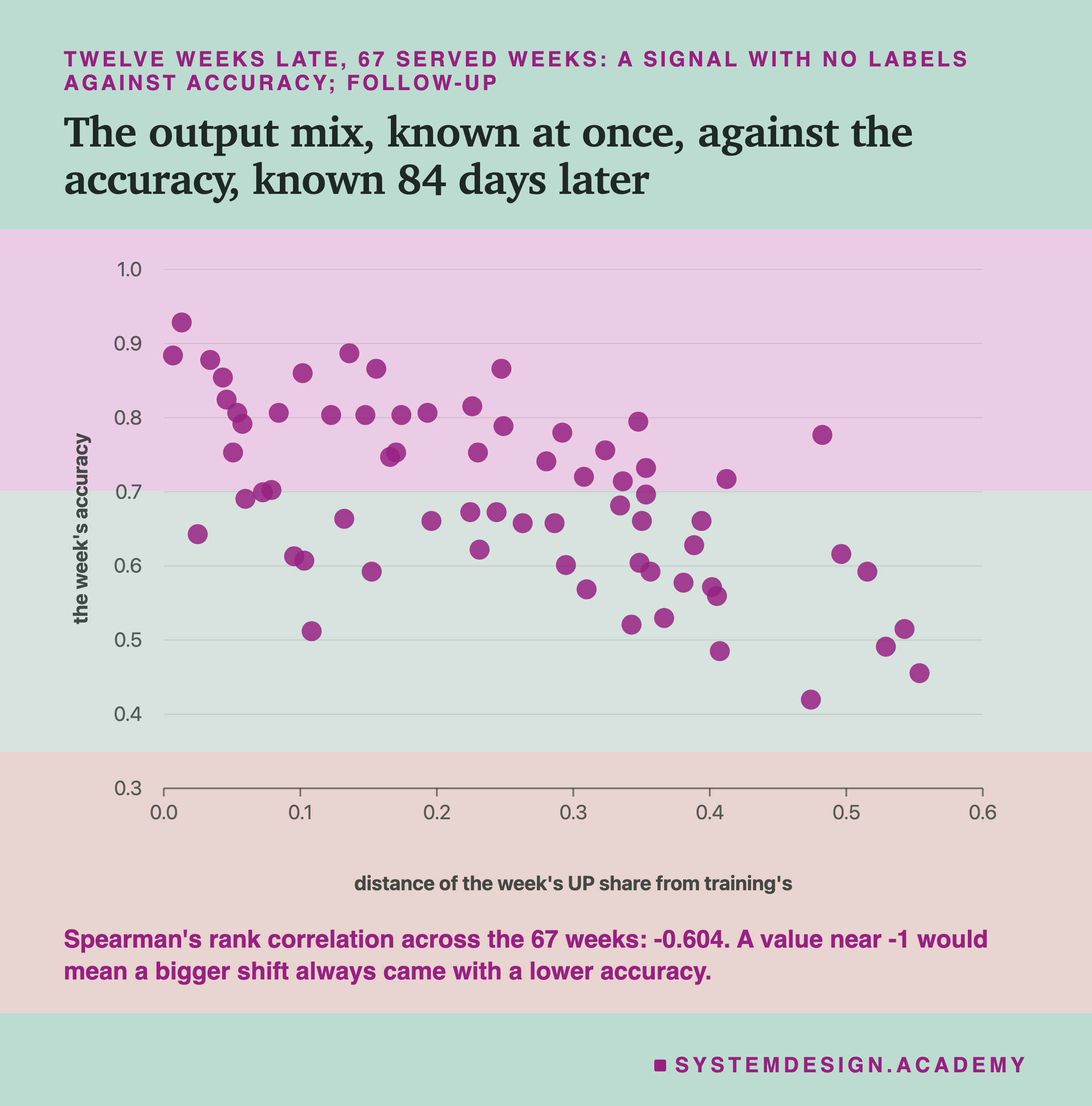
The output mix compares the share of UP answers in a week with the share of UP among the labels the serving model was trained on. If the model suddenly says UP far more or far less often than the world did in training, something may be wrong. Twelve weeks late, the weeks with a larger shift did tend to score lower. The rank correlation (Spearman's, a number from −1 to +1 that says how well one list's order matches another's, with −1 meaning the larger one always went with the smaller other) was −0.604. At the other delays it was between −0.406 and −0.586.
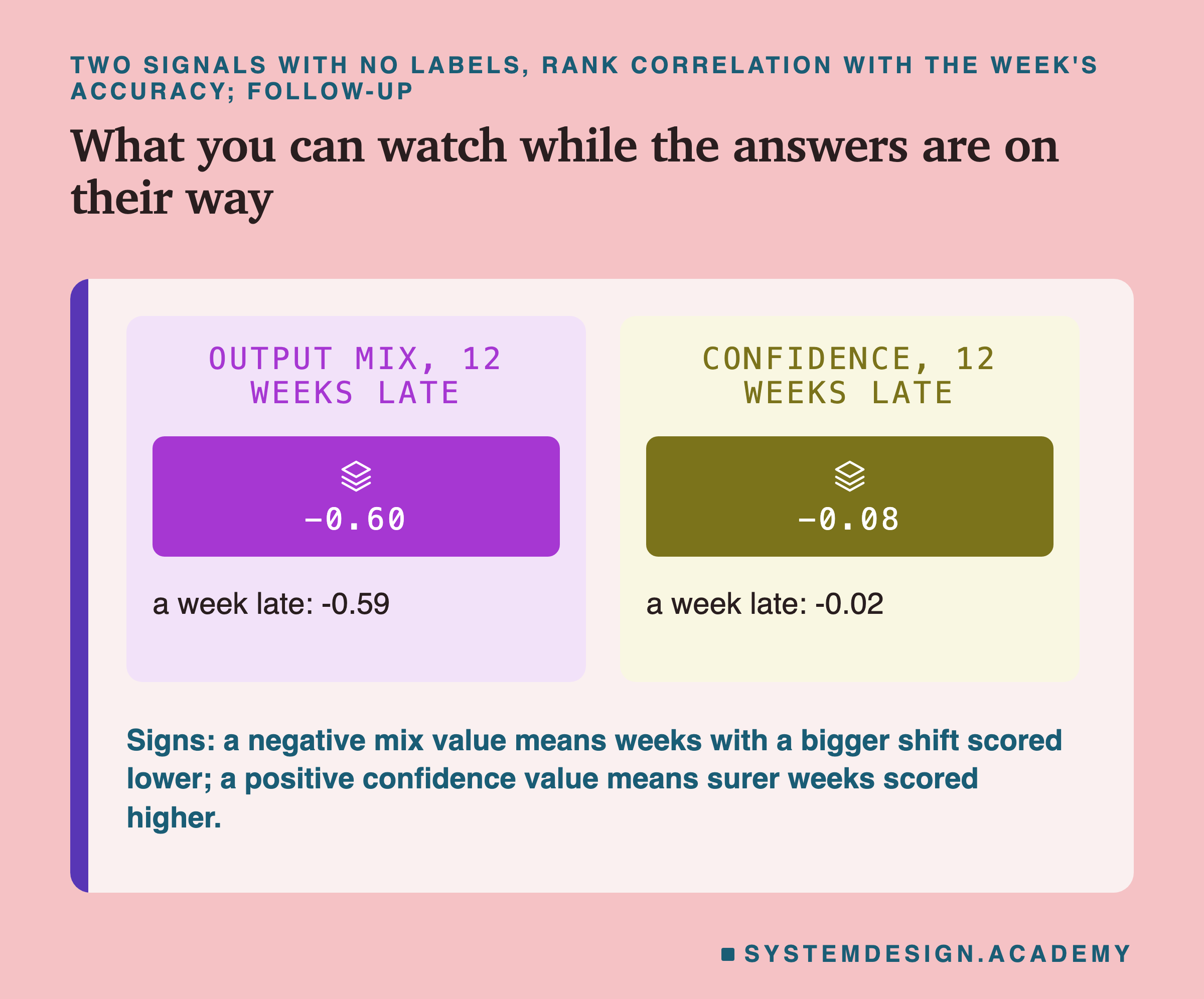
Confidence did much worse. Across the delays its rank correlation with the week's accuracy was weak, between −0.199 and −0.017: the model was about as sure of itself in its bad weeks as in its good ones. That is a warning. A model's own certainty is not evidence that it is right.
A correlation of −0.6 is a real signal, and a weak alarm. Look at the scatter: the seven weeks with the largest shift did mostly score low, but one of them scored 0.777, and among the 28 weeks with a small shift, some scored near 0.51. The output mix is worth watching while you wait, as lesson 7 said, and worth treating as a reason to look closer, not as a measurement of accuracy. I chose these two signals in the follow-up's design because they are cheap; I did not try the many other drift checks that exist.
The Rule That Needs Fresh Answers
Every lesson in this chapter has come back to persistence, the rule of lesson 1 that says "whatever the last half-hour was". It scored 0.8622 on these same 22,656 half-hours, 9.86 points above the best model in this lab. Here it has a new meaning.
Persistence does not learn anything, so it has no retrains and no training rows. It uses exactly one thing: the most recent label. That makes it the purest possible example of a model that depends on fast feedback. With a delay of half an hour it is the best answer on this data. With a delay of a day it would have to repeat yesterday's label at the same half-hour, a different and weaker rule that lesson 1 measured at 0.6741 on its own test rows. With a delay of twelve weeks it would be almost meaningless.
The general point is that a label delay does not only slow down retraining. It removes a whole family of inputs and rules: anything built from recent right answers. On data where the recent past predicts the near future well, as it does on this market, those are often the strongest inputs a team has. Before accepting a long label delay as a fact of life, it is worth asking what a faster label, even a partial one, would unlock beyond the retrains.
What I Would Do With Late Labels
Here is what the lab points to, in the order a team meets it.
Measure the delay, as a distribution. Find out how long your labels really take: not the typical case, but the spread. A delay that is usually a day and sometimes a month behaves like both. This lab used one fixed delay per run, which is simpler than real feedback.
Replay your schedule with that delay before trusting it. Everything in this lab ran on stored history. Doing the same on your own history prices your delay directly: here, a week cost 3.37 points, and the replay found it.
Label every accuracy with its age. A dashboard should never say "accuracy, last 7 days" when it means "accuracy of a week that ended 84 days ago". Put the date range the number describes next to it. Here, twelve weeks late, the unlabelled chart would have misled someone on 65 days one way and 94 days the other.
Watch the output mix while you wait, and trust it only a little. It moved with accuracy here, at −0.6, which is enough to trigger a closer look and not enough to replace the labels.
Look for an earlier label. A first missed payment arrives before a default; a customer's first complaint arrives before a cancellation. A rough early label can support monitoring and early retrains, as long as the team knows what it is.
Compare with a never you could really have had. A baseline from another experiment, trained with fresher labels than yours, flatters every late retrain. Here that mistake turned a loss at twelve weeks, 0.6954 against 0.7077, into an apparent gain of 3.45 points.
Check what your inputs do with time. Here the date input added 1.09 points with fresh labels, 0.7636 against 0.7527, and nothing twelve weeks late, 0.6954 against 0.6962. Test a model with and without such an input before deciding either way.
Try It Yourself
This script is the lab made small. It downloads the same data and runs the weekly retrain twice, with labels half an hour late and twelve weeks late. For each it prints the accuracy over the served half, the worst full week, the served day that week ended, and the day its last label arrived. Then it prints persistence. It does not need a GPU.
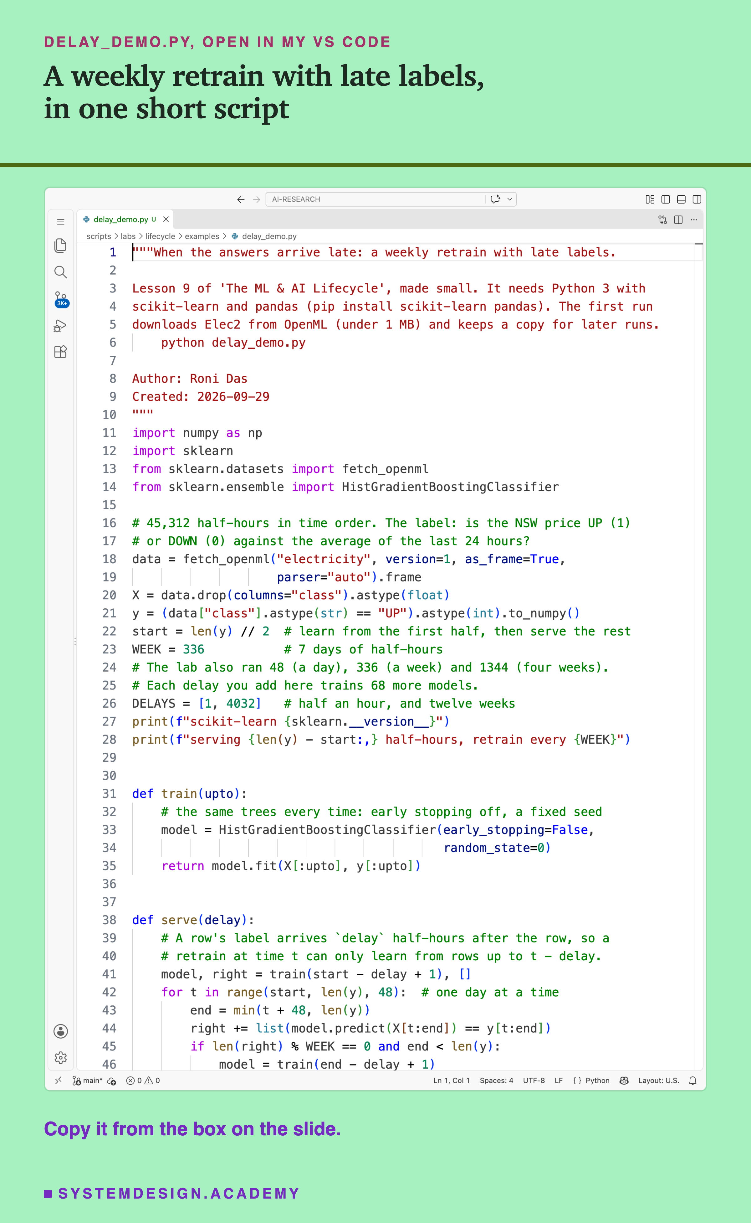
Before you run this lab. You need Python 3 and two libraries: pip install scikit-learn pandas. scikit-learn holds the model and the download, and brings NumPy with it; pandas holds the table. The first run downloads Elec2 from OpenML (under 1 MB compressed), so it needs an internet connection once; scikit-learn keeps a copy in a folder in your home directory (scikit_learn_data) for later runs. To keep it short, it runs two of the lab's five delays; each delay trains 68 small models, so 136 in all. On this Mac it took about 2 minutes, while other jobs were running, so treat that as rough. I ran it with scikit-learn 1.9.1. scikit-learn runs the same way on Windows and Linux, but I have not checked the numbers there, and another version of scikit-learn may give slightly different trees; that is why the first line printed is the version.
"""When the answers arrive late: a weekly retrain with late labels.

Lesson 9 of 'The ML & AI Lifecycle', made small. It needs Python 3 with
scikit-learn and pandas (pip install scikit-learn pandas). The first run
downloads Elec2 from OpenML (under 1 MB) and keeps a copy for later runs.
    python delay_demo.py

Author: Roni Das
Created: 2026-09-29
"""
import numpy as np
import sklearn
from sklearn.datasets import fetch_openml
from sklearn.ensemble import HistGradientBoostingClassifier

# 45,312 half-hours in time order. The label: is the NSW price UP (1)
# or DOWN (0) against the average of the last 24 hours?
data = fetch_openml("electricity", version=1, as_frame=True,
                    parser="auto").frame
X = data.drop(columns="class").astype(float)
y = (data["class"].astype(str) == "UP").astype(int).to_numpy()
start = len(y) // 2  # learn from the first half, then serve the rest
WEEK = 336           # 7 days of half-hours
# The lab also ran 48 (a day), 336 (a week) and 1344 (four weeks).
# Each delay you add here trains 68 more models.
DELAYS = [1, 4032]   # half an hour, and twelve weeks
print(f"scikit-learn {sklearn.__version__}")
print(f"serving {len(y) - start:,} half-hours, retrain every {WEEK}")


def train(upto):
    # the same trees every time: early stopping off, a fixed seed
    model = HistGradientBoostingClassifier(early_stopping=False,
                                           random_state=0)
    return model.fit(X[:upto], y[:upto])


def serve(delay):
    # A row's label arrives `delay` half-hours after the row, so a
    # retrain at time t can only learn from rows up to t - delay.
    model, right = train(start - delay + 1), []
    for t in range(start, len(y), 48):  # one day at a time
        end = min(t + 48, len(y))
        right += list(model.predict(X[t:end]) == y[t:end])
        if len(right) % WEEK == 0 and end < len(y):
            model = train(end - delay + 1)
    return np.array(right)


for delay in DELAYS:
    right = serve(delay)
    weeks = [right[w:w + WEEK].mean()
             for w in range(0, len(right) - WEEK + 1, WEEK)]
    worst = int(np.argmin(weeks))
    last_day = 7 * worst + 6          # served days count from 0
    seen = last_day + delay / 48      # when its last label arrives
    print(f"label delay {delay:>4}: accuracy {right.mean():.4f}")
    print(f"  worst week {worst}: {weeks[worst]:.4f}, ends day "
          f"{last_day}, known day {seen:.0f}")

persist = y[start - 1:-1] == y[start:]  # say what the last half-hour was
print(f"persistence, needs delay 1: {persist.mean():.4f}")
The Lab Report
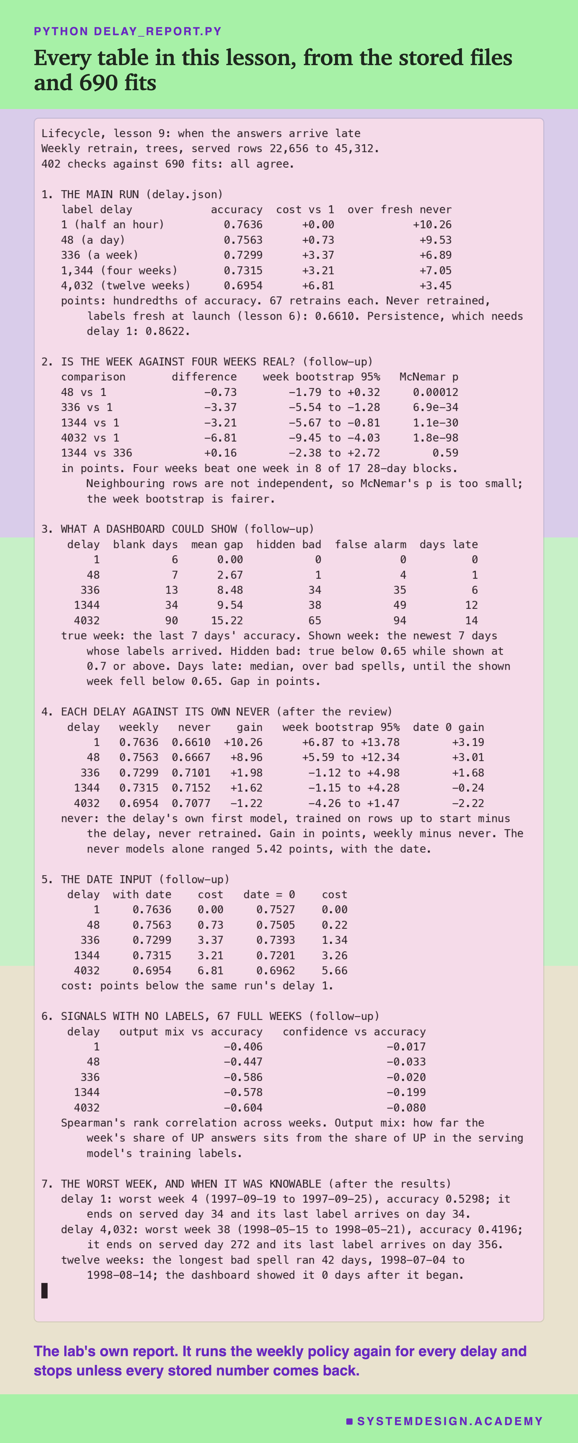
The report lives in scripts/labs/lifecycle/delay_report.py. It reads the lab's stored files, results/delay.json and results/delay_followup.json, results/delay_fairnever.json, lesson 6's results/retrain.json and results/retrain_followup.json, and the Elec2 data from scikit-learn's local copy. The lab stored accuracies, not each answer, so the report runs the weekly policy again for all five delays, with and without the date input, 680 fits in all, and fits the ten fair "never" models of the review check below, 690 in all. It stops unless every stored number comes back exactly: each accuracy, retrain count and 28-day block, every day of the monitoring view, every noise comparison including its 2,000 bootstrap draws, every no-date accuracy, every week's signals, and every accuracy and block of the fair never. It makes 402 checks in all, and they all agree. It changes nothing in the lab's files.
Its json mode writes every number to , which the figures read. The mode checks the student script's stored run, and the mode writes the playground below and checks that it gives the lab's numbers.
Look at a Late Dashboard Yourself
This box has no model in it. It holds, for every one of the 22,656 served half-hours, the real label and the answer of the weekly model under each of the five delays, as two hexadecimal digits per row (counting in sixteens, with the digits 0 to 9 and a to f). From those it can compute any accuracy in this lesson, and the true and shown week for any day and delay. The report checked that every accuracy, every day of the true and shown weeks, and the disagreeing rows between a week and four weeks match the lab's files. It runs in your browser.
As it is, the box prints the accuracy for each of the five delays, 0.7636, 0.7563, 0.7299, 0.7315 and 0.6954, the same as the lab. Then it looks at served day 300 with labels twelve weeks late: the true week was 0.5923, while the dashboard could show 0.7560. That is one of the 65 hidden bad days.
Then try true_week(day, delay) and shown_week(day, delay) for other days and delays, and look for a day where they disagree most. Try accuracy(4032, 48 * 266, 48 * 273) to score the twelve-week run's worst week, served days 266 to 272. And try only_right(336, 1344) and only_right(1344, 336): the two numbers that decided the "inversion".
The Code, Part by Part
Loading. fetch_openml("electricity", version=1) downloads Elec2 once and reads the local copy after that. The label column holds the words UP and DOWN, turned into 1 and 0. start is the middle row: the model learns from everything before it and serves everything after it. WEEK is 336 half-hours.
train. It builds the boosted trees with early_stopping=False and random_state=0, so the same rows always give the same model, and fits them on rows 0 up to upto. The slice X[:upto] stops just before row upto.
serve. This is the whole lesson in ten lines. The first model trains on rows up to start - delay + 1, so its newest row is delay half-hours before serving begins. Then the loop serves one day, 48 half-hours, at a time, and records whether each answer was right. Every time a full week has been served, it retrains, but only up to end - delay + 1: the rows whose labels have arrived. With delay equal to 1, that is every row served so far, exactly lesson 6's weekly policy.
How to Price a Label Delay
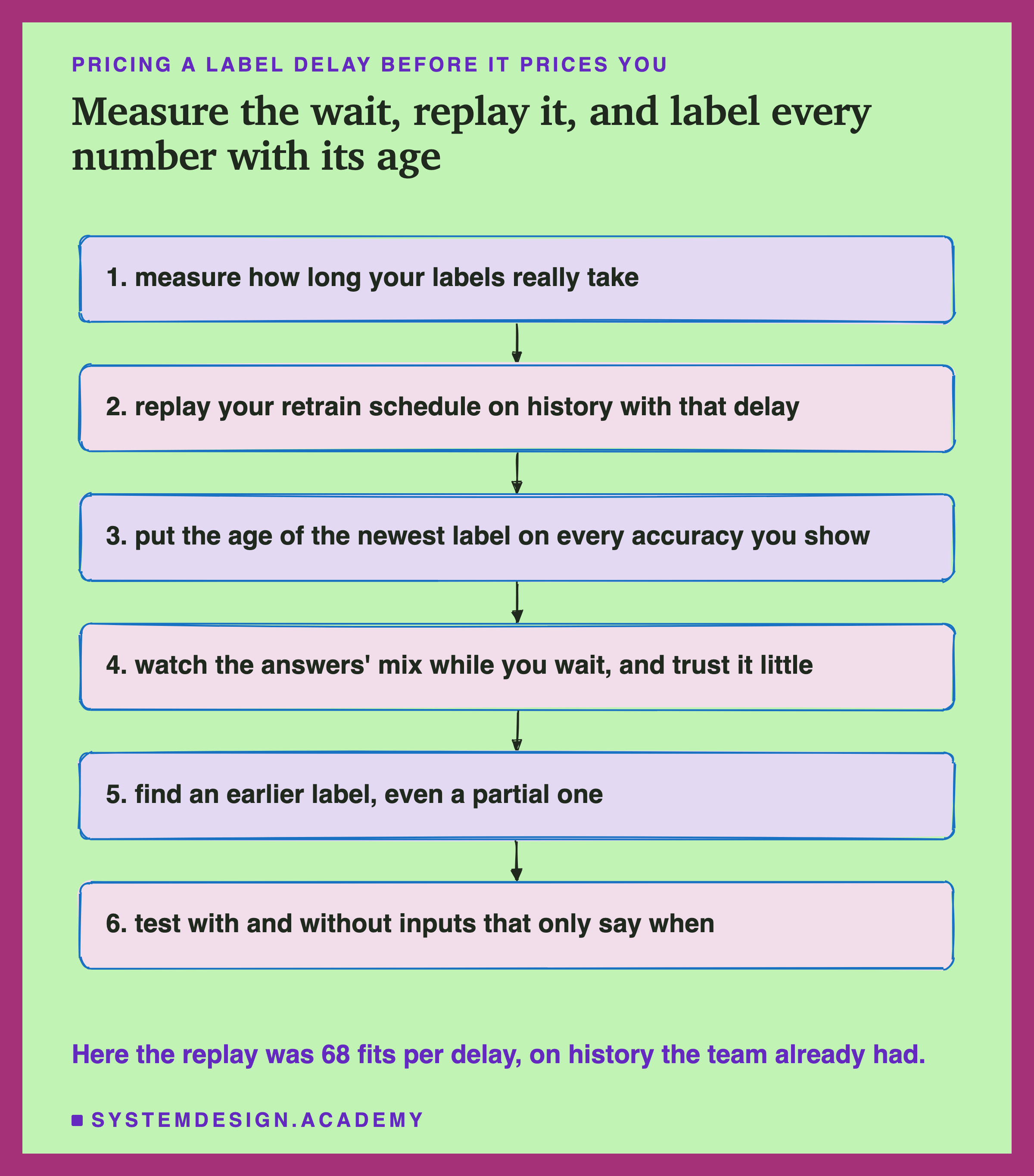
Measure how long your labels really take. Pull the time between each prediction and its label from your own logs, and look at the whole spread, not the average.
Replay your retrain schedule on history with that delay. Serve the stored history in time order, retrain on the schedule you use, and cut each retrain off at its time minus the delay. Compare with a replay at the shortest delay you could get. That difference is what the delay costs you, in your own units.
Put the age of the newest label on every accuracy you show. Every chart of live accuracy should say which dates it describes. If the newest complete week is 84 days old, the chart should say so in its title.
Watch the answers' mix while you wait, and trust it little. It is free and immediate. Here it tracked accuracy partly, at a rank correlation of about −0.6. Use it to decide where to look, not what to conclude.
Find an earlier label, even a partial one. An early sign of the final answer can drive monitoring and faster retrains. Keep the true label for the final scoring.
Test with and without inputs that only say when. Here the date added 1.09 points with fresh labels (0.7636 against 0.7527) and nothing twelve weeks late (0.6954 against 0.6962). Measure both before you keep or drop one.
Retrain on Late Labels, or Find a Faster Signal?
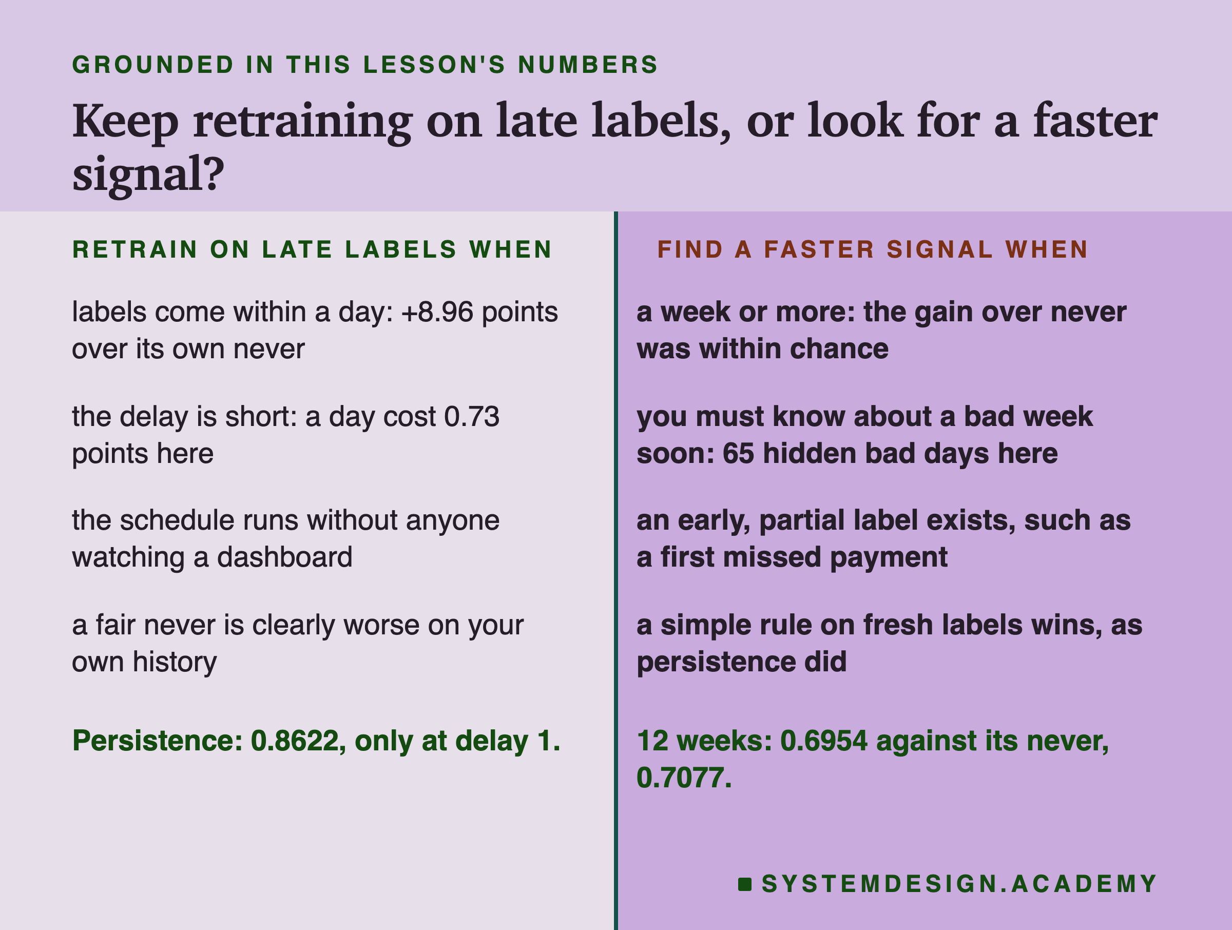
Keep retraining on late labels when they arrive within about a day. Here, a day late, weekly retraining beat the never the same team could have had by 8.96 points.
Keep retraining when the delay is short. A day late cost 0.73 points here, and even that could not be told apart from chance.
Keep it when the schedule must run on its own. A schedule does not need a dashboard to decide anything, so a late dashboard does not stop it.
Keep it when a fair never is clearly worse on your own history. Replay both at your real delay and compare.
Look for a faster signal when the delay is weeks. A week cost 3.37 points here, and from a week on, the gain over never retraining could not be told apart from chance. Twelve weeks late, retraining scored 0.6954 against never's 0.7077.
Look for one when you must know about a bad week soon. Twelve weeks late there were 65 hidden bad days. Only a faster label, or a you trust, shortens that.
Look for one when an early, partial label exists, such as a first missed payment or a first complaint.
And look for one when a simple rule on fresh labels would win, as persistence, at 0.8622, did here only because the label came back in half an hour.
What These Numbers Can and Cannot Tell You
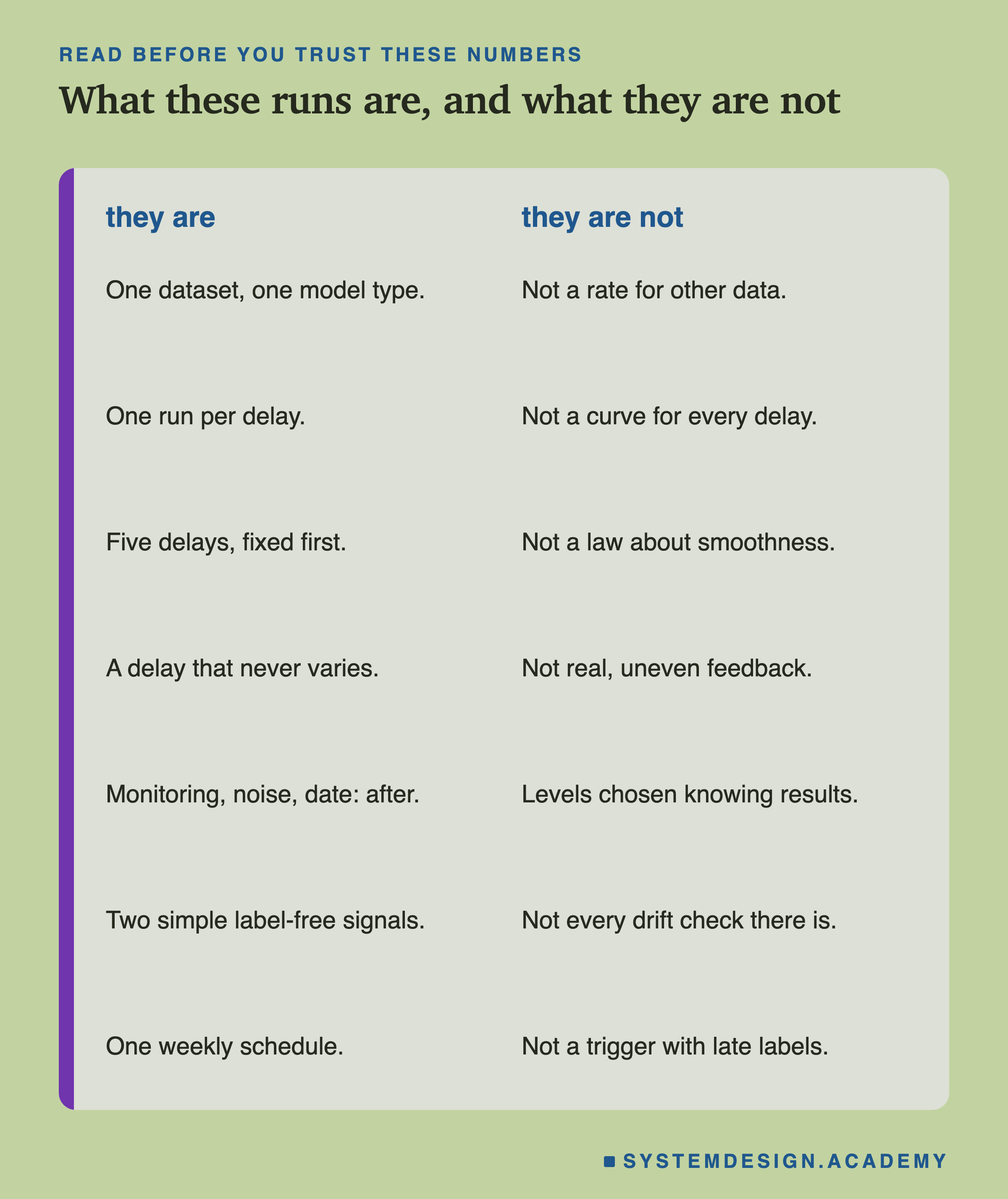
One dataset, one model type, one run per delay. Everything here is one electricity market and one kind of model, retrained on one schedule. How much a delay costs depends on how fast the world moves and how much the newest rows teach. For a slow-moving problem, twelve weeks might cost nothing; for a fast one, a day might cost a great deal.
Five delays, fixed before the run. I did not measure the delays in between, so I cannot draw a smooth curve, and the one kink I found, a week against four weeks, cannot be told apart from chance.
A delay that never varies. Every label in a run arrived exactly the same time after its row. Real feedback is uneven: some labels come quickly, some late, some never. That can cause its own problems, such as a model that learns mostly from the cases whose labels come back fastest, which this lab cannot show.
The follow-up came after. The monitoring view, the levels 0.65 and 0.70, the noise tests, the no-date runs and the two signals were designed after I saw the main results, and written down before they ran. The block counts and the worst weeks were worked out after all the results. The fair never was designed after a review of the draft, and written into the lab file before it ran.
Two simple signals, one schedule. I tested only the output mix and the confidence, not the many other drift checks. And I did not run a trigger with late labels; lesson 6's reasoning that a trigger would be hurt twice is still reasoning, not a measurement.
What to Do Next
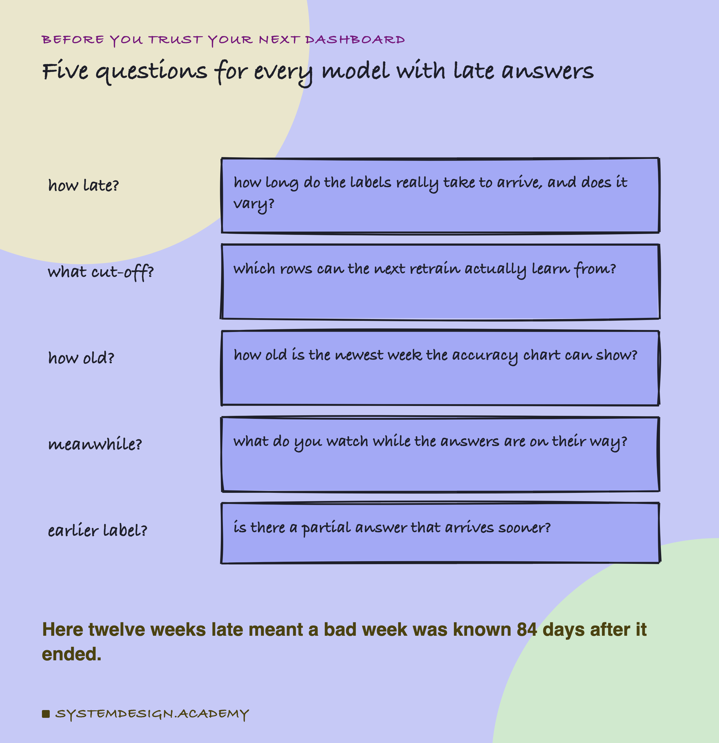
Pick one model your team has in service and answer the five questions on the card. The first is the one most teams skip: find out, from your own logs, how long the labels actually take to arrive, and how much that varies. Everything else follows from that number.
Then open the chart your team uses to watch the model's accuracy, and check what dates its newest point describes. If the answer is "some weeks ago", change the title so that nobody reads it as today. That costs nothing, and here, twelve weeks late, it was the difference between a chart that told the truth about the past and one that misled people about the present on 159 days.
The chapter plan's last lesson puts the whole lifecycle together as one loop, with the measured failure at each step.
Knowledge Check
Knowledge Check
4 questions - Score 80% to pass
With labels twelve weeks late, the weekly retrain scored 0.6954 against 0.7636 with labels half an hour late. What made the difference?
Four weeks late scored 0.7315 and one week late 0.7299. What does the lesson conclude from that?
Twelve weeks late, why did the dashboard show a fine week on 65 days when the real week was bad?
Which signal, available with no labels at all, moved with the week's accuracy in this lab?