The Piano Tuner
Imagine a school with an old piano in its hall. A piano slowly goes out of tune: the strings stretch a little every week, the room gets warmer and colder, and children play it hard. Nobody notices one week's change. After a few months, everyone notices.
The school has two ways to decide when to call the tuner. The first is a calendar: the tuner comes on the first Monday of every month, whether the piano needs it or not. That costs money every month, and some visits are wasted, but the piano is never out of tune for long.
The second way is to listen. The caretaker plays a short tune every Friday and calls the tuner only when it sounds clearly worse. That sounds smarter, because the school pays only when there is a problem. But the caretaker has to decide what "worse" means. Worse than what? He decides to compare each Friday with the first Friday after the last tuning.
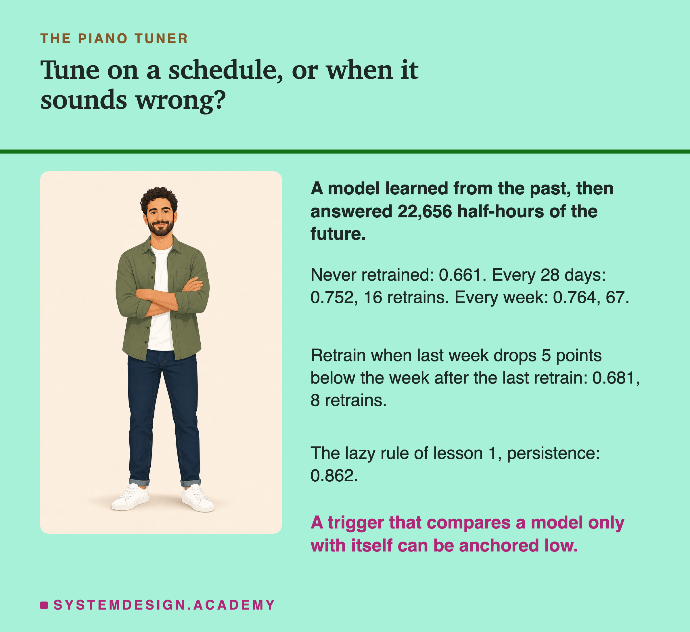
Now suppose one tuner does a poor job, on a damp week, and the piano already sounds bad on the first Friday after. From then on, the caretaker compares every Friday with that bad Friday. The piano never sounds much worse than that, so he never calls anyone again. The rule looked careful. It was anchored to a bad day: tied to one starting point that happened to be poor.
This lesson is about the same decision for a program that learns from examples. I tried both ways, a calendar and a listening rule, on real data, and the listening rule failed in this same way.
Where This Lesson Starts
This chapter follows one model through its life, on the same data, one step at a time. Start with the dumbest model set the baselines, the simple rules a model must beat. Same code, different model showed that two training runs of the same code can give two different models. Picking the best of many showed how the winner of a search can do worse later. The promotion gate measured the check that decides whether a new model replaces the old one, and canary and shadow measured how much live traffic it takes to see that a new model is worse.
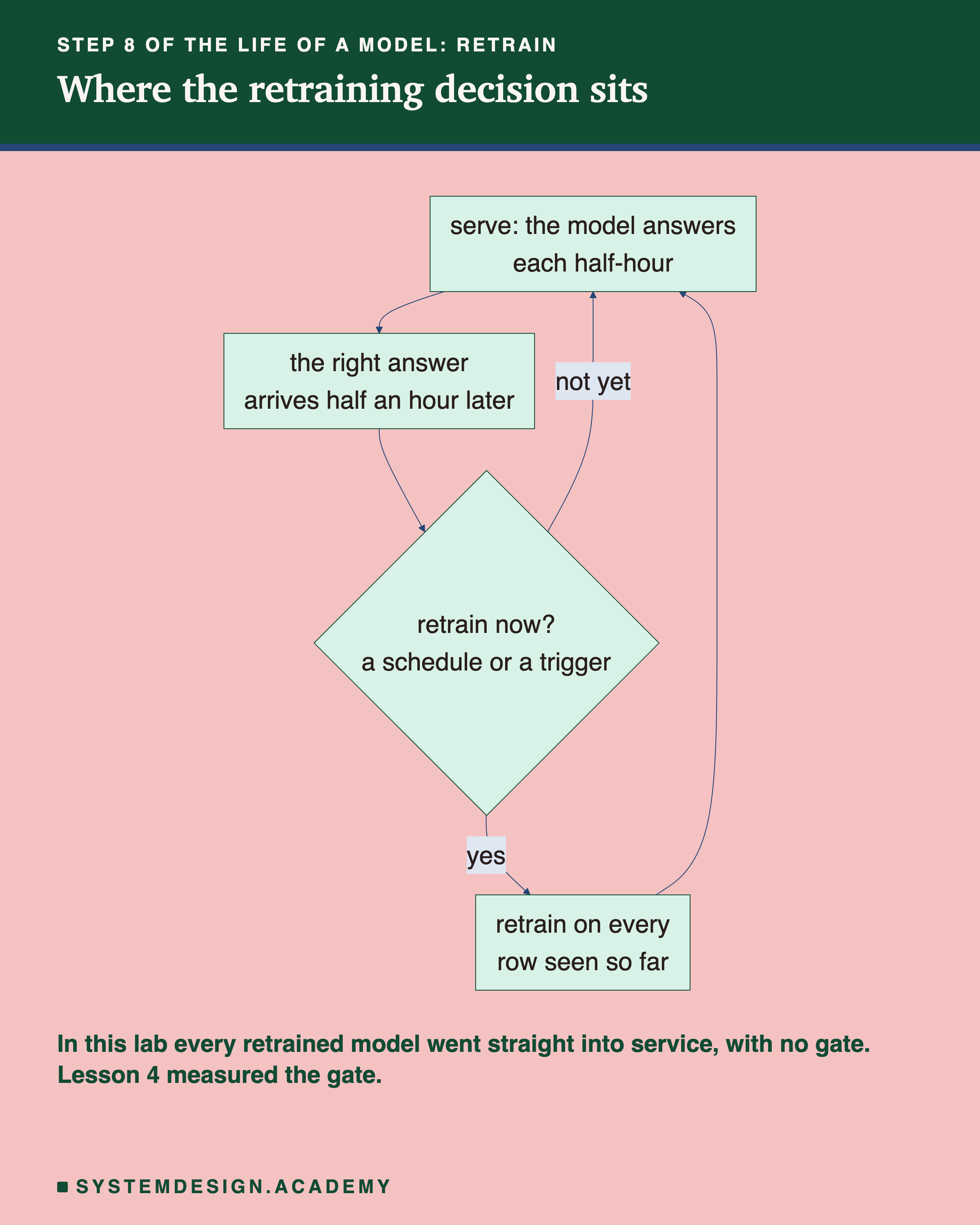
Now the model is live and has been answering for a while. The question is when to train it again. The course's lesson on training pipelines and orchestration has a slide called "When Should the Pipeline Run?". It describes, in words, a schedule, a trigger on new data, a trigger on input drift (the inputs moving away from what the model saw in training), and continuous retraining. I will not repeat it. This lesson measures a schedule and a third kind of trigger that slide does not cover: a trigger on the model's own measured accuracy, which needs the right answers to arrive. It also counts what each one costs.
The chapter before this one also touched retraining. Its lesson tomorrow is different trained a model on one year of bike rentals and compared "never retrain" with "retrain every month". It found that retraining helped a great deal, but only through one input, the year. I will come back to that finding, because this lab found something related and different.
Eight Words for This Lesson
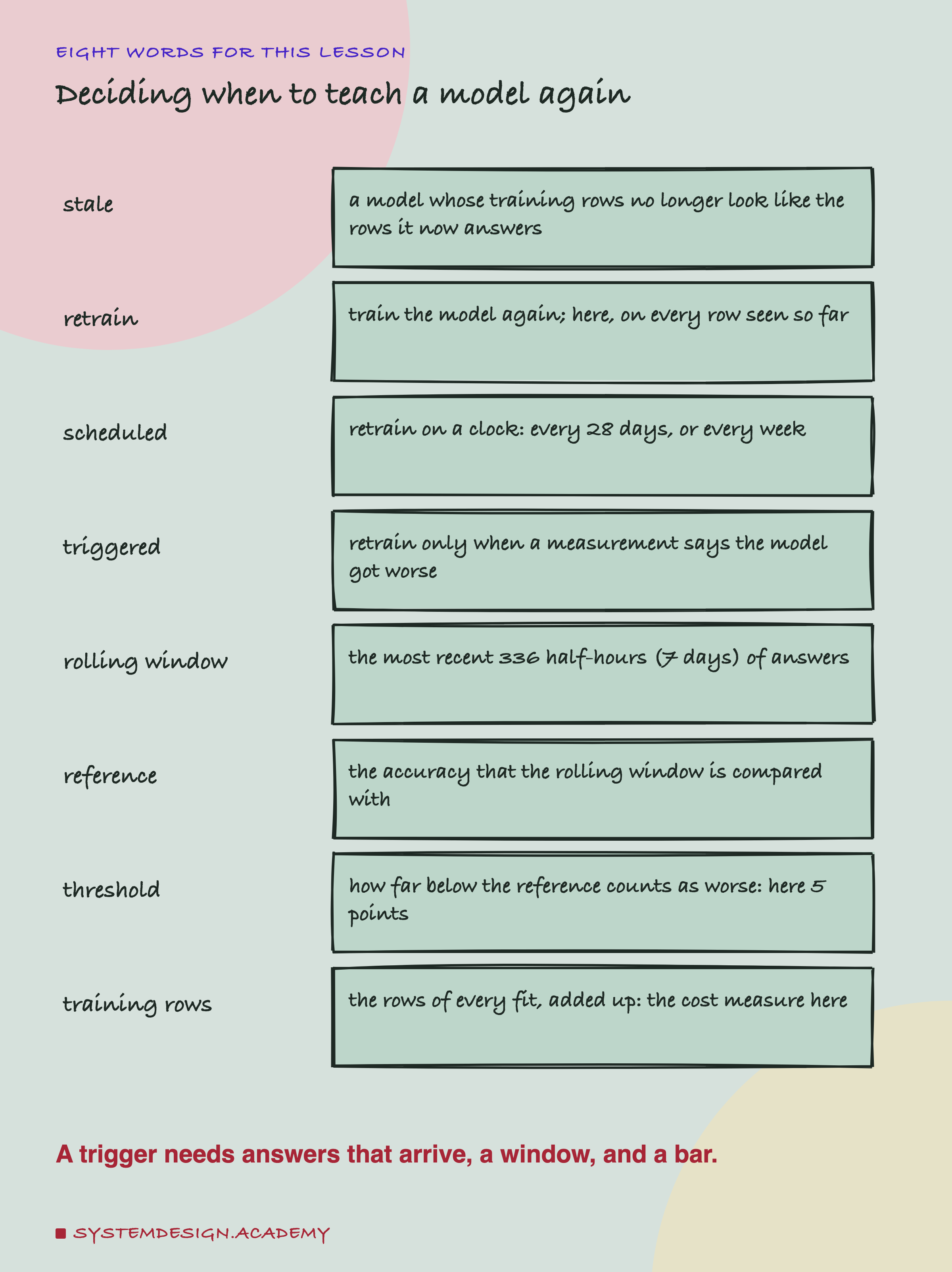
A model is stale when the rows it learned from no longer look like the rows it now answers. To retrain is to train it again; in this lab, a retrain always learns from every row seen so far. Scheduled retraining happens on a clock, whatever the model is doing. Triggered retraining happens only when a measurement says the model got worse.
A trigger needs three things. The first is the right answers, called labels, because you cannot measure accuracy without them. The second is a rolling window: the most recent stretch of answers you measure over, here the last 336 half-hours, which is 7 days. The third is a bar: a reference level to compare with, and a threshold, how far below the reference counts as worse. Here the threshold is 5 points, where a point is one hundredth of accuracy, the share of answers that were right.
To fit a model is to train it once on a set of rows. The cost of retraining here is counted in training rows: for every fit, the number of rows it learned from, all added up. I did not time anything, so the lesson never talks about seconds.
Why a Model Goes Stale
A trained model is a summary of its training rows. It learned which inputs went with which answers, in the months it saw. Then the world keeps moving. Prices rise, habits change, a new competitor arrives. The model does not know any of that. It keeps answering as if it were still the last day of its training.
Here is what that looked like in this lab. I trained boosted trees (many small yes-or-no decision trees, each built to fix the mistakes of the ones before, as in lessons 1 to 5) once on the first half of the data and let them answer the second half, 22,656 half-hours, without ever retraining. The chart below shows how often the frozen model said UP in each block of 28 days, against how often the price really was UP.
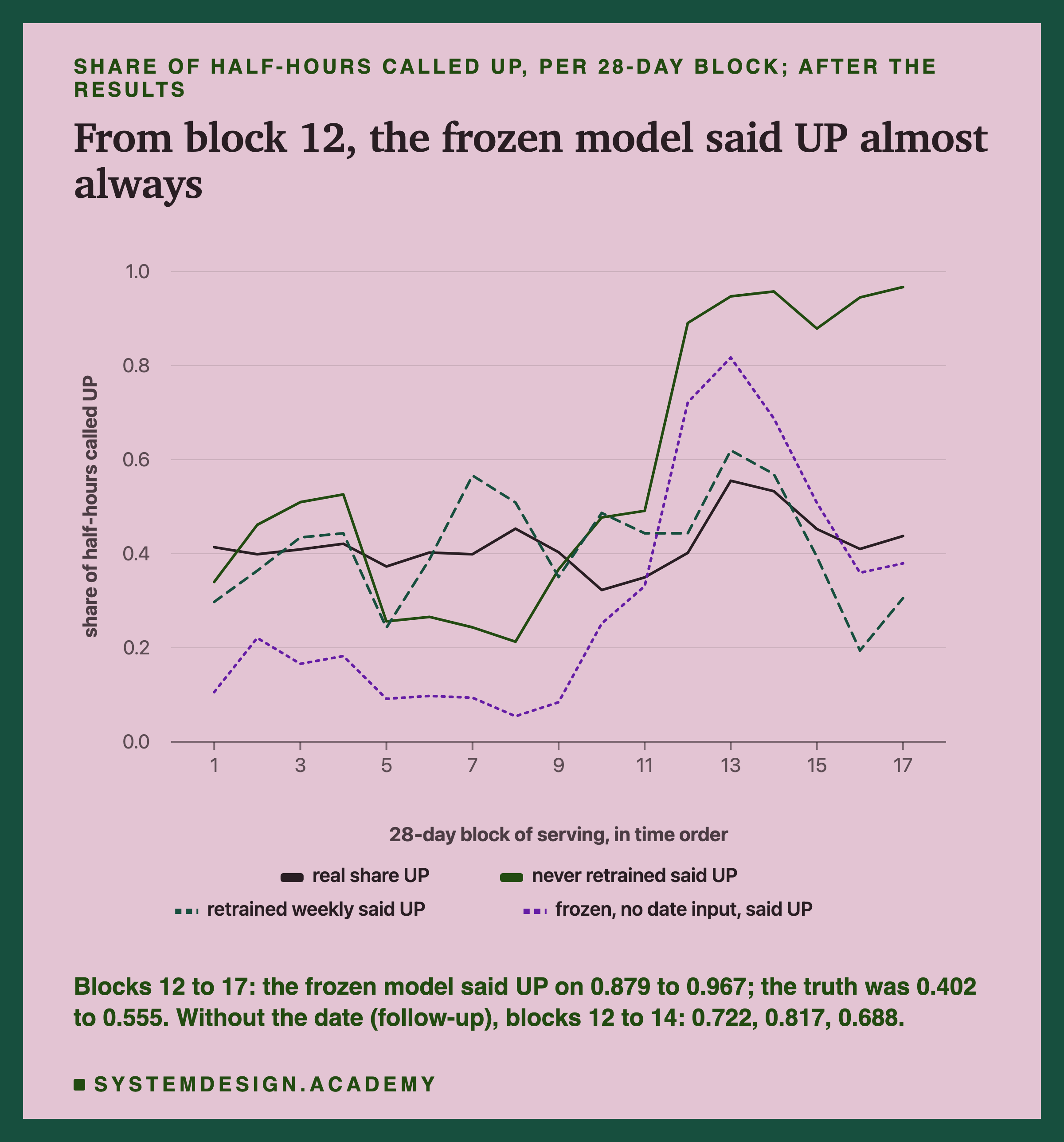
The frozen model never matched the truth closely. In blocks 5 to 8 it said UP too rarely (0.213 to 0.266 against a truth of 0.373 to 0.453), and in blocks 10 and 11 too often. Then, at block 12, which starts on 26 June 1998, it jumped: it said UP on 0.879 to 0.967 of half-hours to the end, while the real share was 0.402 to 0.555. A model that says UP on 96.7% of half-hours when 43.8% are UP is not predicting any more. I measured this after I saw the results.
This is the same kind of failure lesson 1 found in July 1998, when the trees said UP on nine rows in ten. A later slide finds the input that most of it came through, and it is not the one I first expected.
Four Ways to Decide
The lab compared four policies. All four were written in the lab file before it ran, and none was changed afterwards.
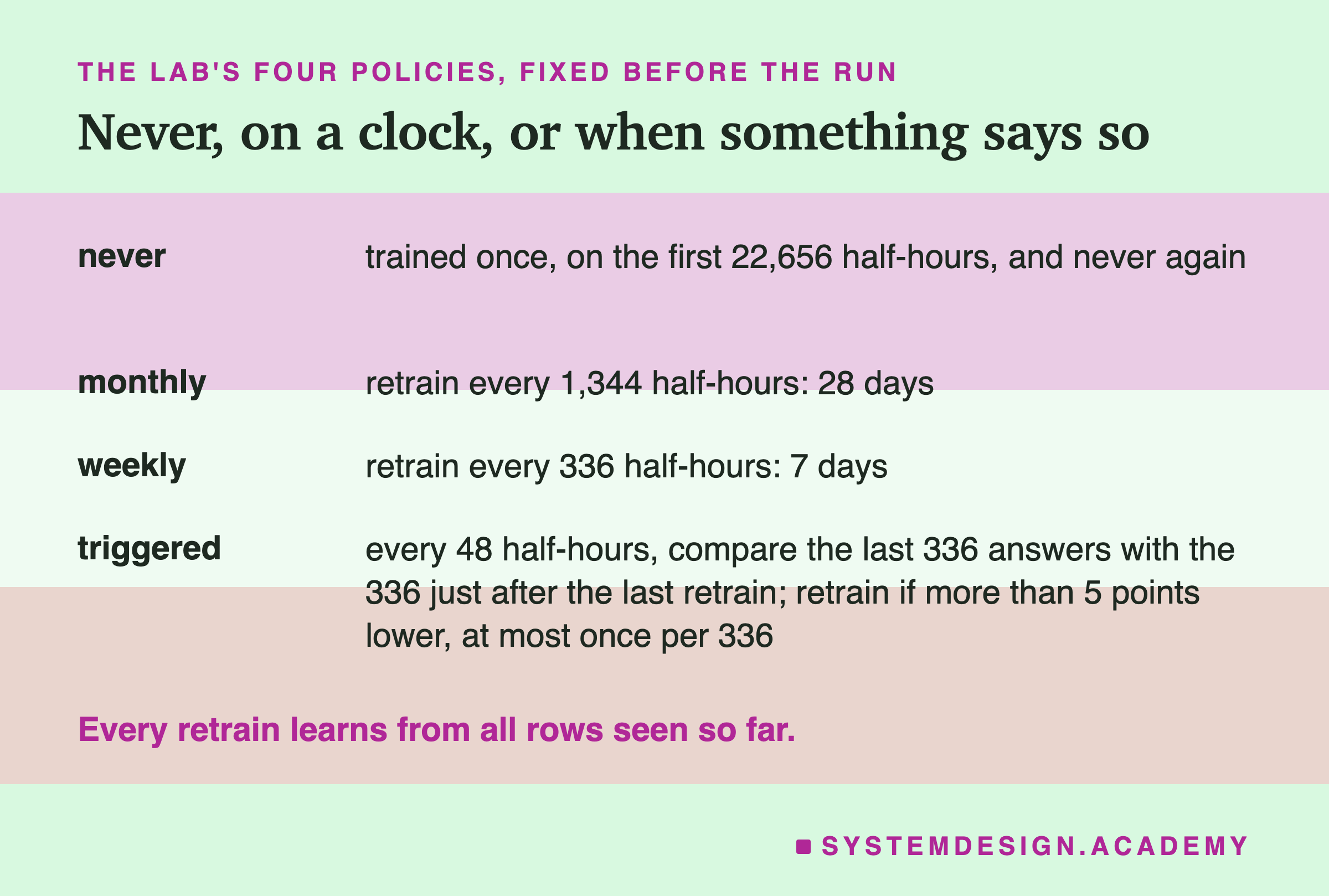
Never is the frozen model. It is the cheapest policy and the baseline for the other three.
Monthly and weekly are schedules. Every 28 days, or every 7 days, the model is trained again on every row seen so far, and the new model takes over at once. I use "monthly" for 28 days so that every block has the same length.
Triggered watches the model. Every day it measures accuracy over the last 7 days and compares it with the model's accuracy over its own first 7 days after it was trained. If the last 7 days are more than 5 points worse, it retrains. It never retrains twice within 7 days.
Notice what the trigger compares with. It compares the model with itself, with how the same model did just after it started. That is a common and natural choice: "has this model got worse since it went live?" The piano caretaker made the same choice. The rest of the lesson shows what that choice cost.
What the Lab Ran
I wrote the lab's design at the top of its file, retrain_lab.py, before it ran. The dated record is in the chapter plan (2026-09-29, "RETRAIN LAB (batch 6) designed before running").
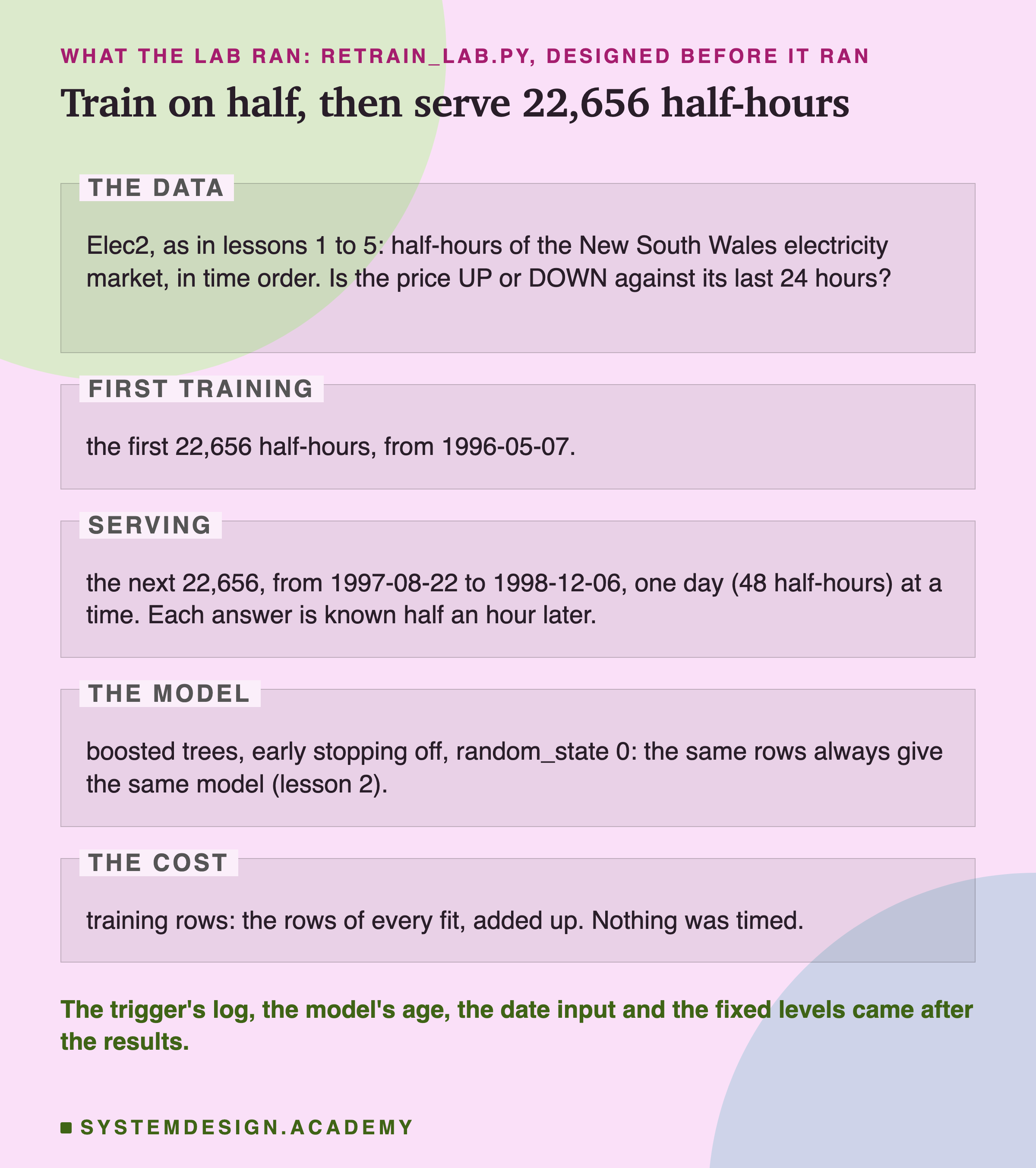
The data is Elec2 again: 45,312 half-hours of the New South Wales electricity market in time order, where each row asks whether the price is UP or DOWN against its average over the last 24 hours. The model first trains on the first half, 22,656 rows, and then answers the second half in time order, one day of 48 half-hours at a time. Each label is known half an hour after the answer, when the next row arrives. The dates are rebuilt from row numbers, as in lesson 1, so the last served day, 6 December 1998, may be a day out: OpenML says 5 December.
The model is the boosted trees from the earlier lessons, with early stopping switched off (early stopping would set aside a random tenth of the training rows) and a fixed seed, the starting number for the model's random choices, random_state=0. Lesson 2 found that with those settings, the same rows always give the same model. So any difference between policies comes from when they retrained, not from luck in training.
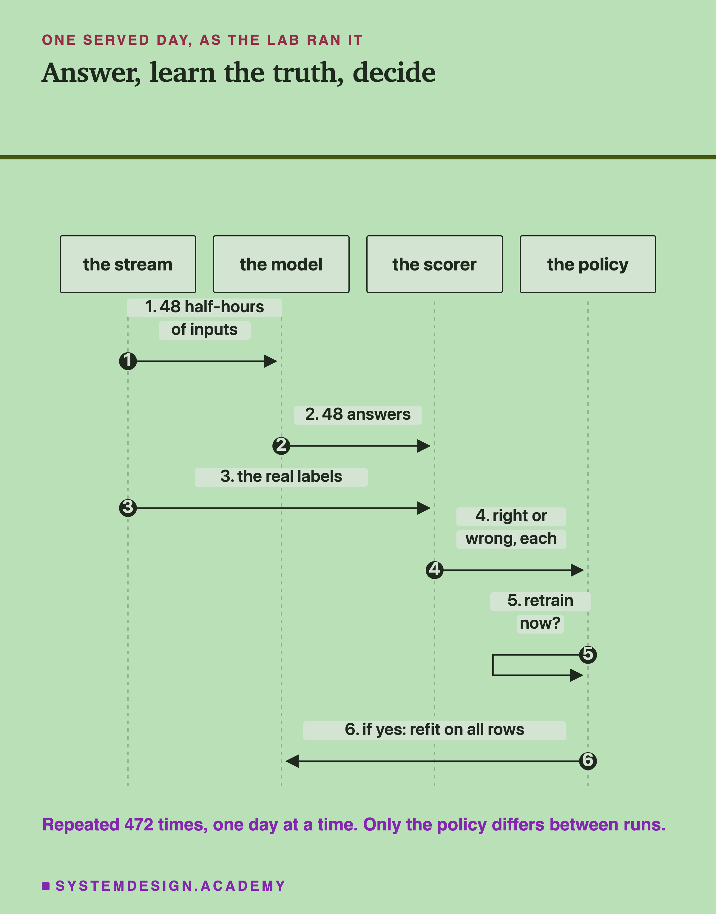
The Main Run
Here is what the lab stored in results/retrain.json.
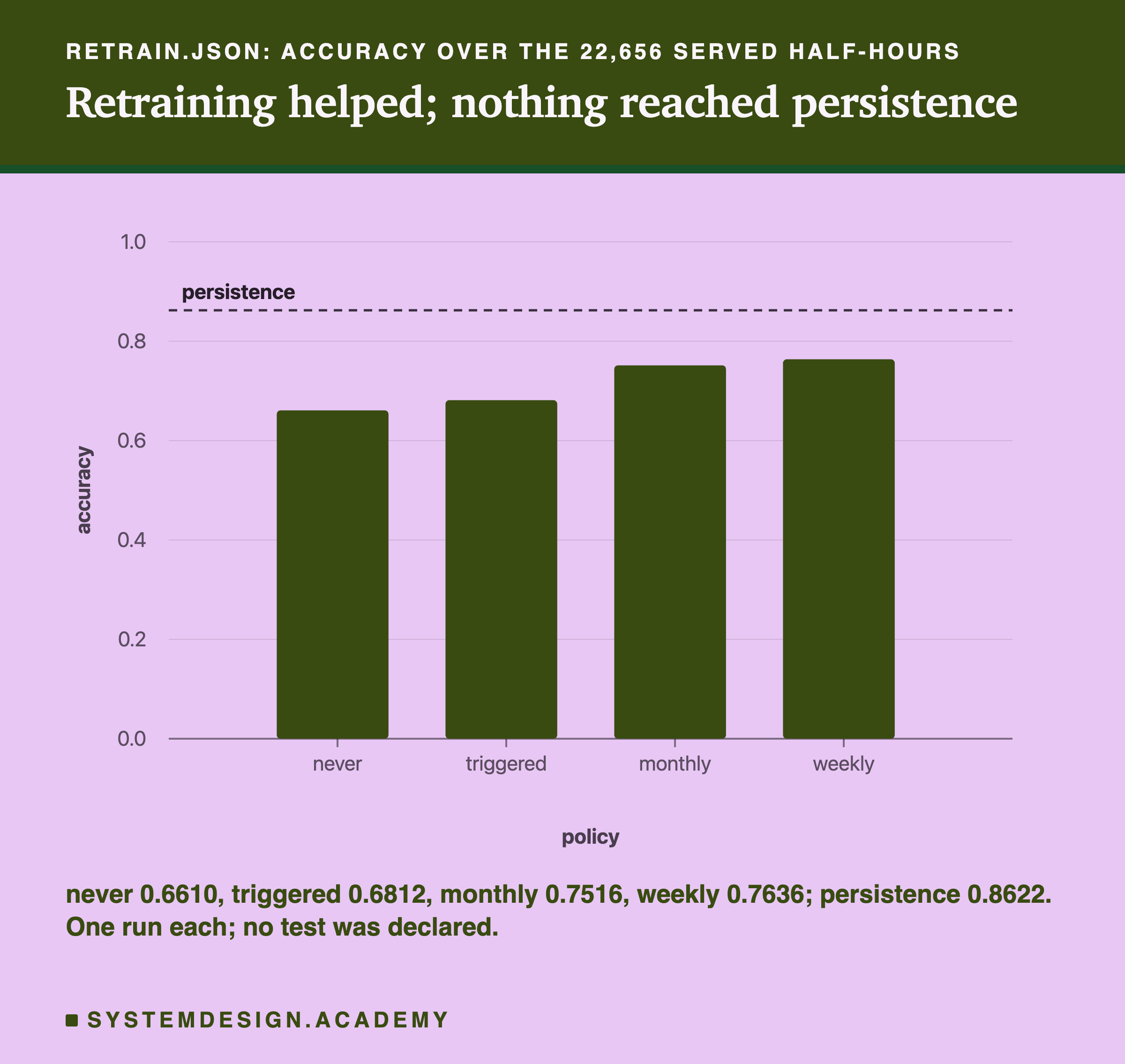
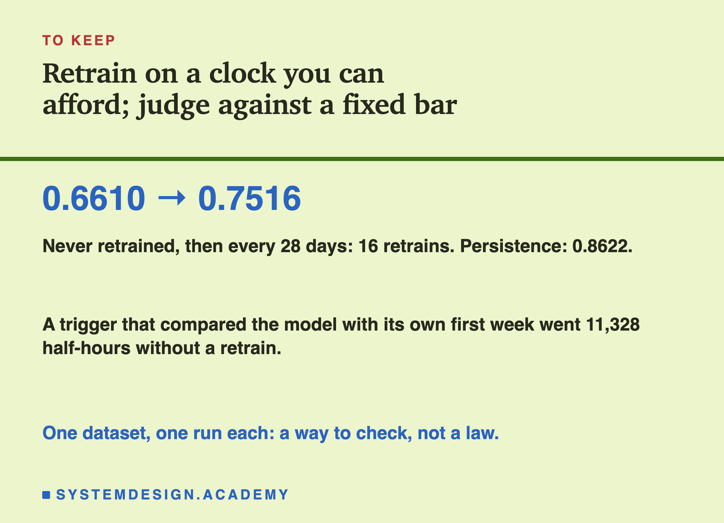
Never scored 0.6610. Monthly scored 0.7516, 9.06 points higher, with 16 retrains. Weekly scored 0.7636, 10.26 points above never, with 67 retrains. Triggered scored 0.6812, only 2.03 points above never, with 8 retrains. And persistence, which learns nothing, scored 0.8622, above all four.
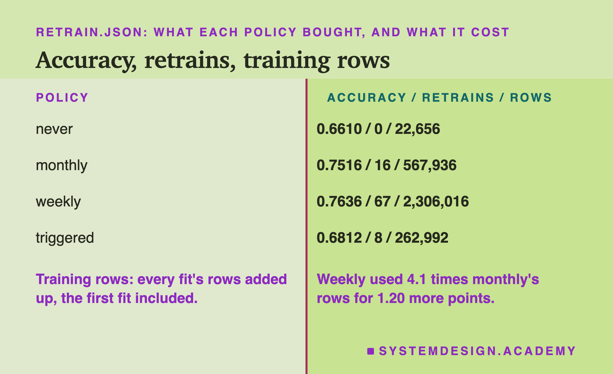
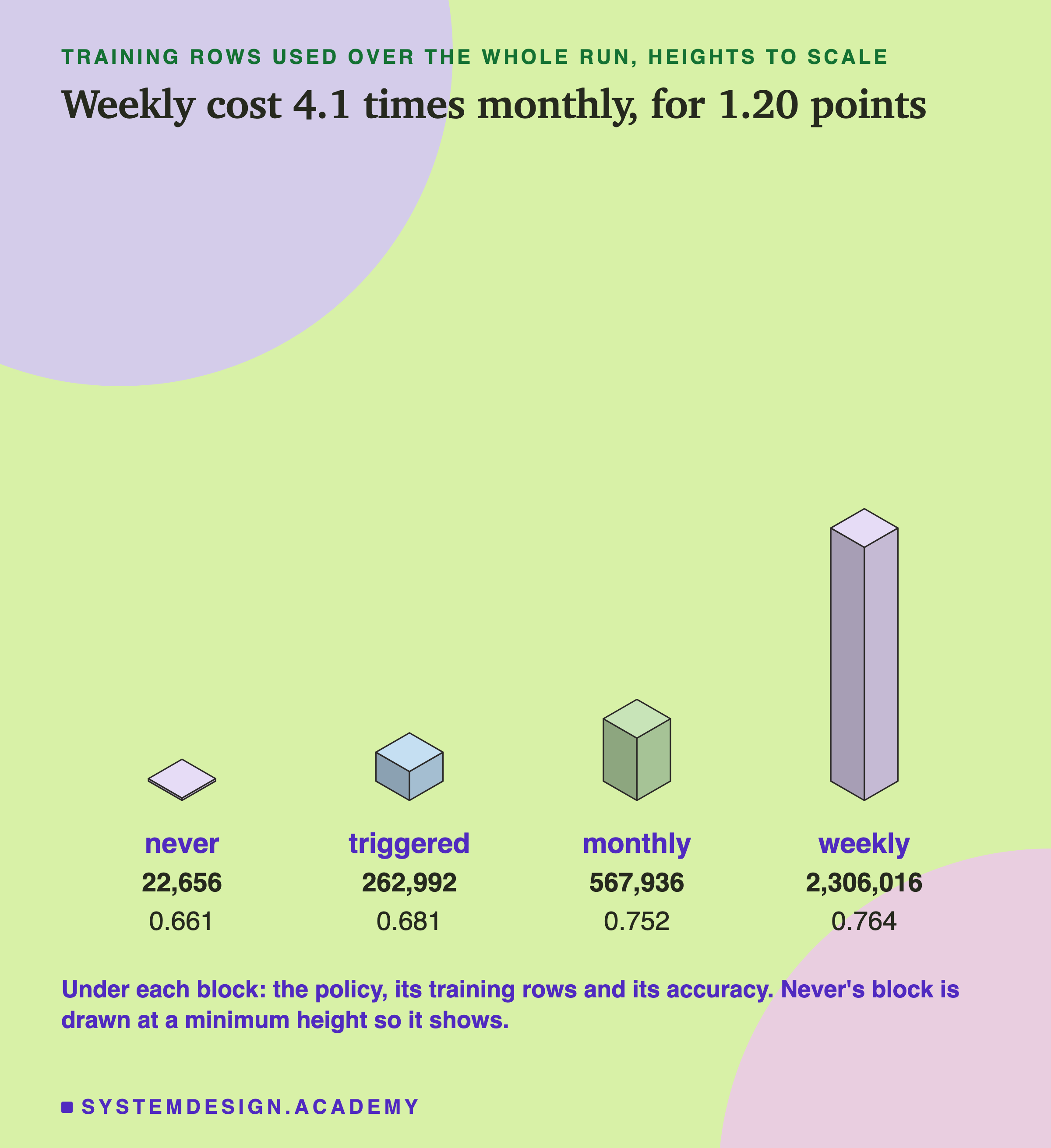
Now the costs. The first training used 22,656 rows, and every policy paid that. With that first fit included, monthly used 567,936 training rows in all, weekly 2,306,016, which is 4.1 times monthly's, for 1.20 more points of accuracy, and the trigger 262,992. The retrains alone were 545,280, 2,283,360 and 240,336 rows. The trigger used the fewest and bought the least.
On the surface, then, retraining on a schedule helped a lot, and retraining more often helped a little more at a much higher cost. The trigger saved rows and lost most of the benefit. The next slides look inside each of these numbers, because that first reading turned out to be only part of it.
Block by Block
One number over 22,656 half-hours hides when things happened. Here is each policy in each block of 28 days.
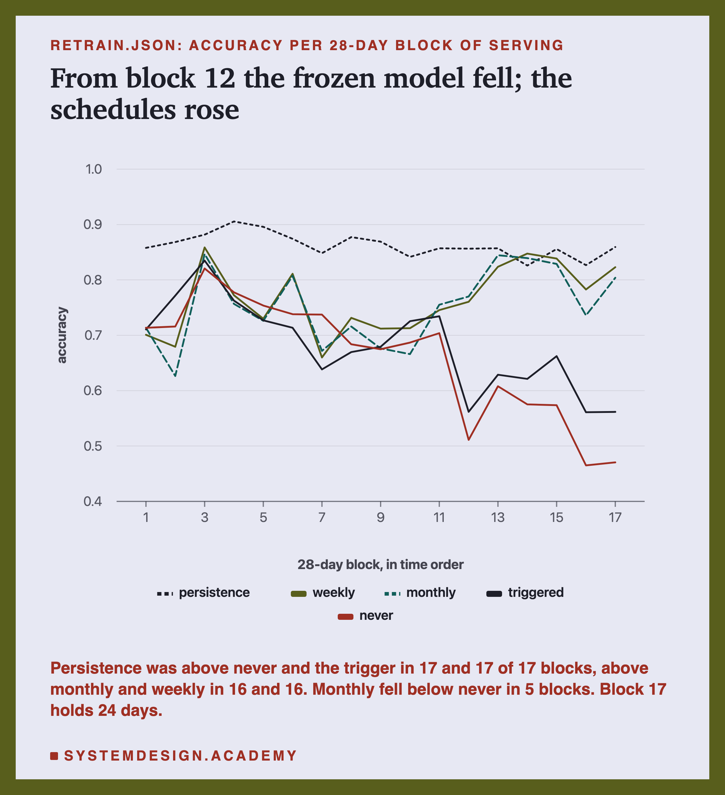
For the first eleven blocks, about ten months, the four policies were close together, and never was often as good as any of them. Then, from block 12, the frozen model dropped sharply: it fell to 0.511 in block 12, and below a coin, 0.465 and 0.470, in blocks 16 and 17. The two schedules went the other way and ended the run between 0.80 and 0.85.
A retrain is not always an improvement. Monthly scored below never in 5 of the 17 blocks, weekly in 5, and the trigger in 6. In block 2, monthly scored 0.626 where the frozen model scored 0.716. Lesson 2 showed that a new model is a different model, and lesson 4 showed that a new model can be worse. Here, with no gate at all, some retrains made things worse for a month.
And persistence was above never and the trigger in all 17 blocks, and above monthly and weekly in 16 of them. Retraining did not change the lesson 1 result: on this data, a rule that learns nothing beats every trained model.
What Each Retrain Bought
A retrain is not free. I did not time these fits; on a large model a retrain can take hours of expensive machines, and every new model needs checking before it goes live. So a useful question is how much each retrain bought. I measured it after the results, as extra rows answered correctly compared with never retraining.
Monthly answered 2,053 more half-hours correctly than never, which is 128.3 per retrain. Weekly answered 2,325 more, but it needed 67 retrains, so each one bought only 34.7. And the step from monthly to weekly bought 272 more correct half-hours for 51 more retrains: 5.3 per extra retrain.
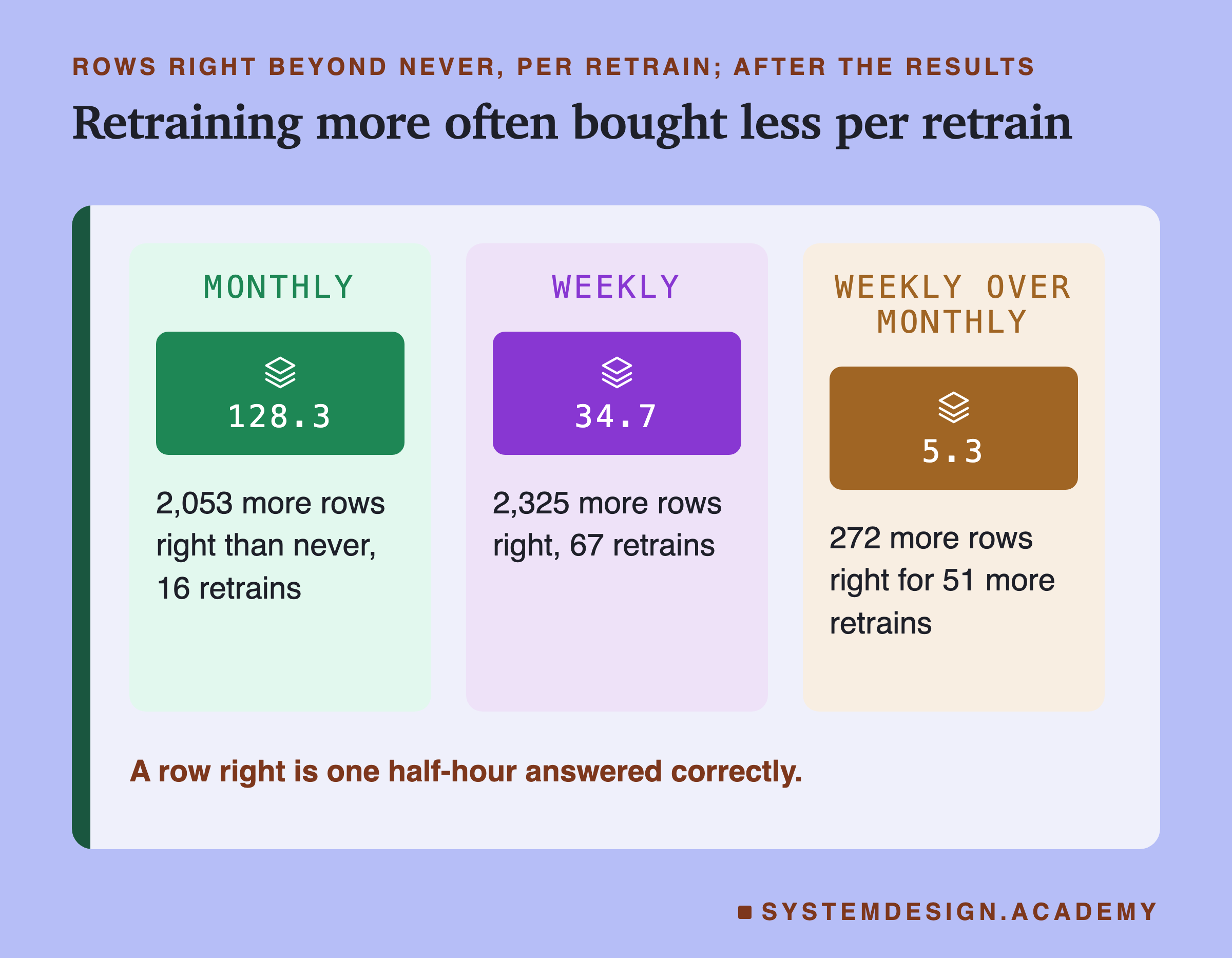
The first retrains closed most of the gap between a stale model and a fresh one; retraining more often added less and less each time. Whether 5.3 extra correct answers per retrain is worth it depends on what a retrain costs you and what a wrong answer costs you. I did not time these fits, so I cannot give their cost in time here. For a model that trains for a day on rented graphics cards (GPUs, the chips large models train on), 51 extra retrains to gain 272 answers out of 22,656 would be difficult to justify.
Does a Model Get Worse Within a Week?
If a model goes stale, then a model that was just retrained should be better than the same model a week later. I checked that after the results, by grouping the weekly policy's answers by how many days had passed since its last retrain.
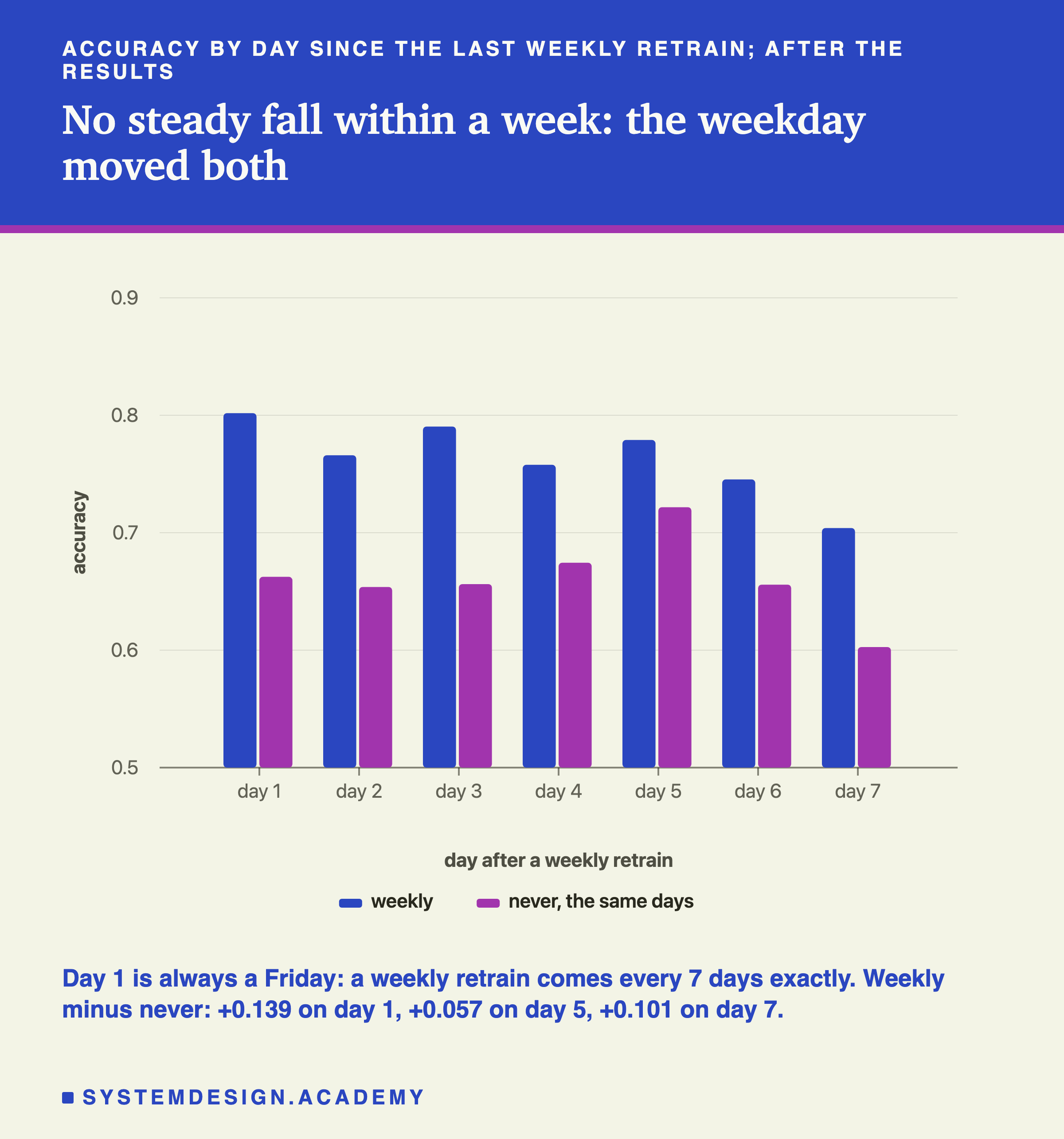
At first the weekly numbers seem to fall: 0.802 on the first day after a retrain and 0.704 on the seventh. But there is a trap. A weekly retrain comes every 7 days exactly, so "day 1 after a retrain" is always the same day of the week, a Friday, and "day 7" is always a Thursday. The fall could be about Thursdays, not about age.
The never model is the control, because it is never retrained, so its "day 7" means nothing except "Thursday". It dips on the same day, from 0.722 on day 5 to 0.603 on day 7. The gap between weekly and never does not fall steadily across the week: +0.139, +0.112, +0.134, +0.083, +0.057, +0.090, +0.101. So within a week I cannot see staleness at all here; what I saw was the weekday. For monthly, whose 28 days cover every weekday equally, the first week after a retrain was the best, +0.123 above never, and the next three were +0.072, +0.100 and +0.067. That is a first-week edge, not a steady decline.
The lesson for reading any "accuracy by age" chart: check that age is not tied to something else, such as the day of the week, before you read the chart as decay.
When the Trigger Fired
The lab stored how many times the trigger fired, not when. So after the results I replayed its policy with the lab's own serving loop, writing down every check. The replay reproduced every stored number.
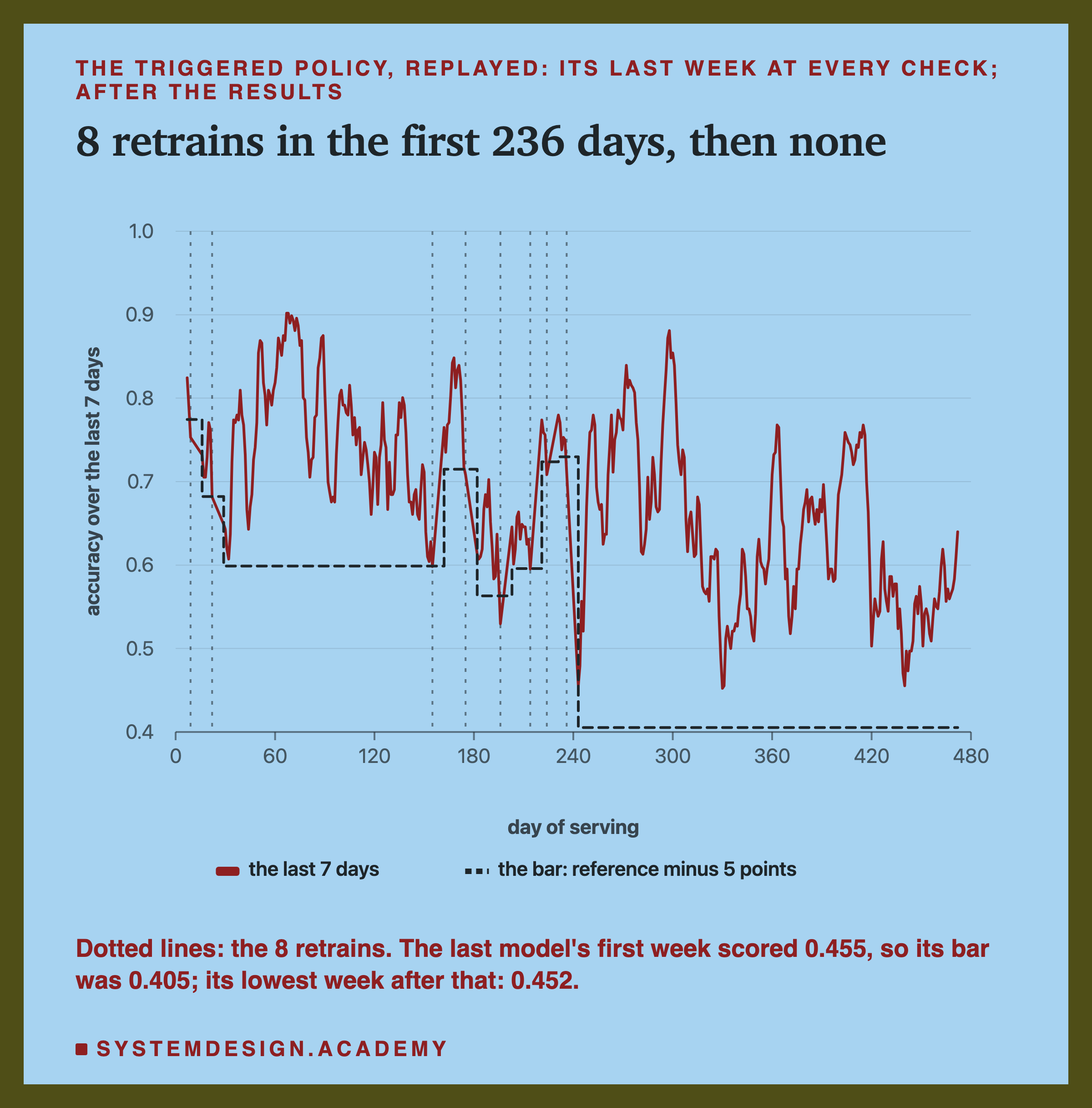
The trigger fired 8 times, all in the first 236 days of serving. It fired at half-hour 432, on 31 August 1997, when the last week scored 0.753 against a reference of 0.824; again on 13 September; then not for four months; then six times between 24 January and 15 April 1998. After 15 April 1998, it never fired again, for the remaining 236 days.
Look at the first firing. The reference was 0.824, a very good first week, and a week of 0.753 was 7.1 points lower. The model had not really broken; its first week was unusually good: 0.824 is above 91% of the frozen model's weekly scores, and its first block averaged 0.714. So the same rule that later failed to fire also fired early for a reason that had little to do with the model getting worse. A reference taken from one week carries that week's luck, good or bad.
Why It Stopped Firing
Here is the model the trigger kept for the second half of the run.
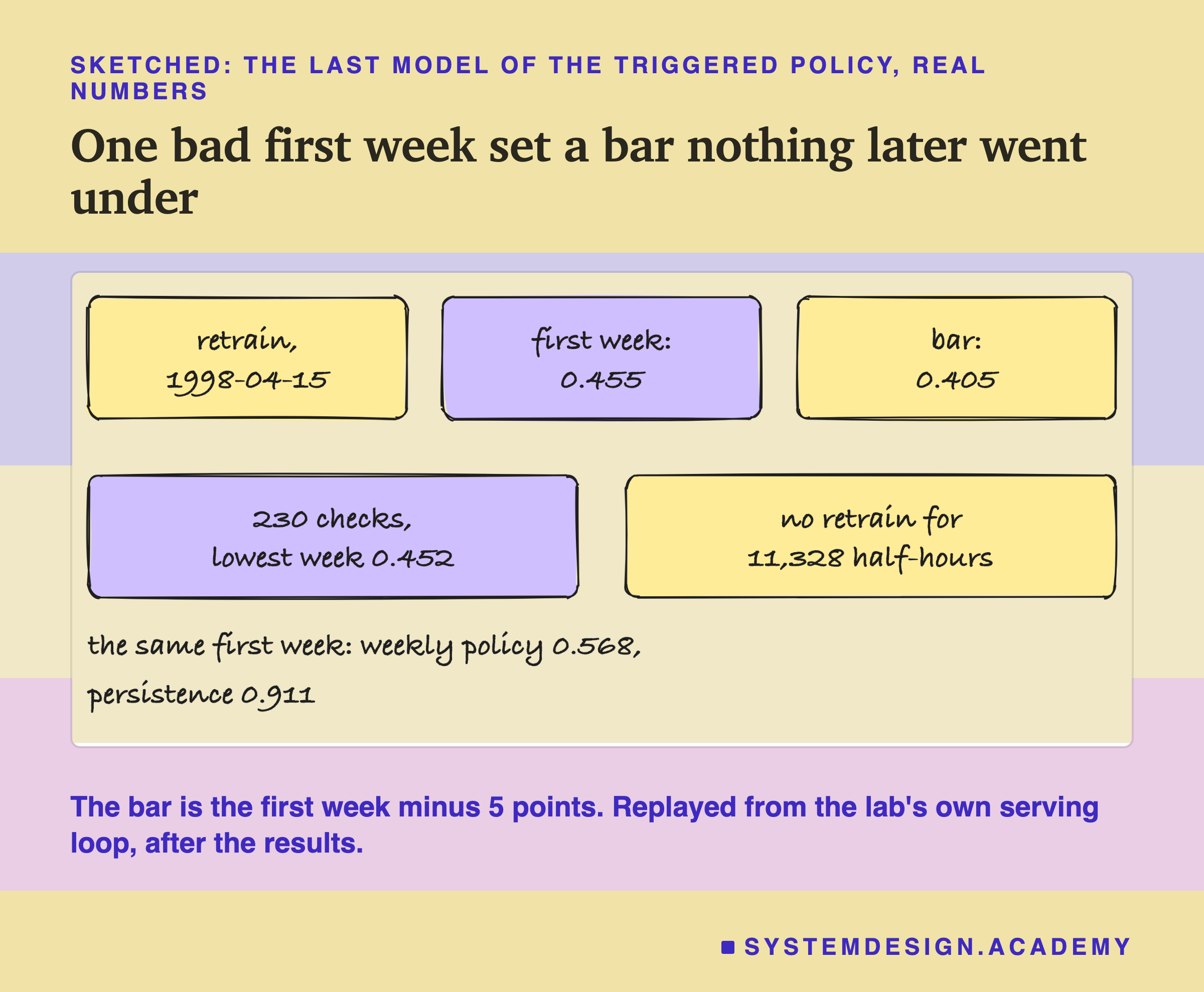
It was trained on 15 April 1998. Its first week scored 0.455, below the 0.5 a coin would get. That first week became its reference, so its bar was 0.405. Over the next 230 daily checks, its last 7 days never went below 0.452, so it never crossed the bar, and it served 11,328 half-hours, half of the whole run, without a retrain. From late June to the end, its 28-day blocks scored 0.561 to 0.662, while the two schedules scored 0.736 to 0.847 in the same blocks.
Was that week just hard? Partly. The weekly policy's model, trained at almost the same time, scored 0.568 on the same week, also poor. But persistence scored 0.911 on it, so the week was not hard for everything. It was hard for these trees. Whatever the reason, the trigger could not see the problem, because it only asked whether the model was worse than itself, and it had been bad from the first day.
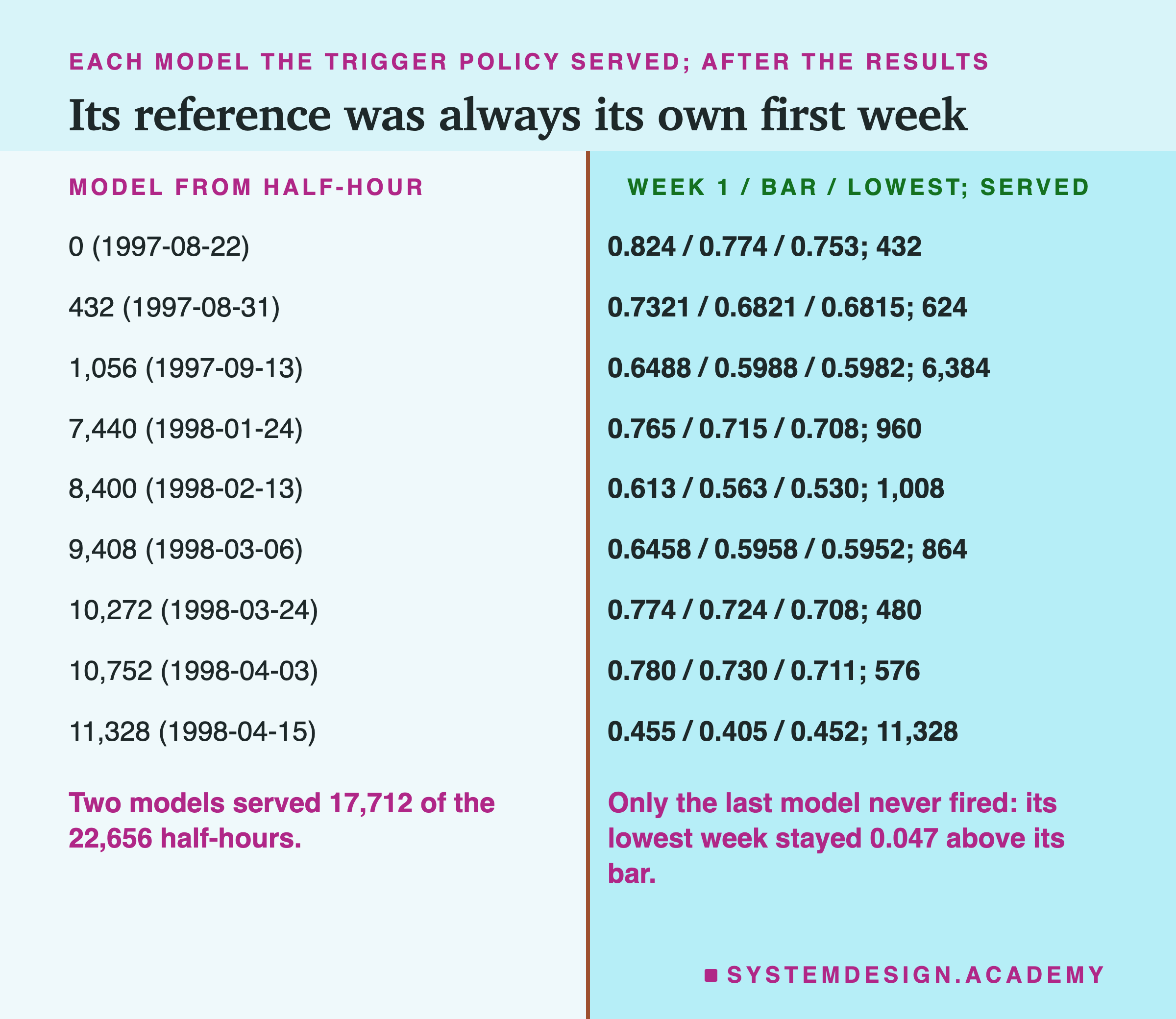
The same thing happened once before, more mildly. The model trained on 13 September 1997 had a first week of 0.649 and served 6,384 half-hours before a week finally fell below its bar of 0.599. Two models with weak first weeks served 17,712 of the 22,656 half-hours between them. So the measured reason the trigger rarely fired is this: its bar was set by each model's first week, and when that week was already bad, the bar sat below almost anything that could happen later. A slow decline is a different story for this trigger: because its reference stays fixed at the model's first week, a gradual fall piles up and does eventually cross 5 points, as it did for the model from 13 September. Only a trigger that compares each week with the week before would miss a slow decline; that is reasoning, and I did not test such a trigger.
A Follow-Up: Fixed Levels
I designed a follow-up after I saw these results, and wrote its design into the lab file's followup mode before it ran. Its results are in results/retrain_followup.json. The question: is the failure a property of triggers, or of this particular reference?
The follow-up tried two other kinds of trigger, with everything else unchanged. The first kind compares the last 7 days with a fixed level instead of the model's own first week: retrain whenever the last 7 days fall below 0.65, or 0.70, or 0.75. The second, which I call the holdout reference, measures the reference before the model starts serving: when training at some moment, it also trains a second model without the latest week and scores it on that week, and uses that score as the reference.
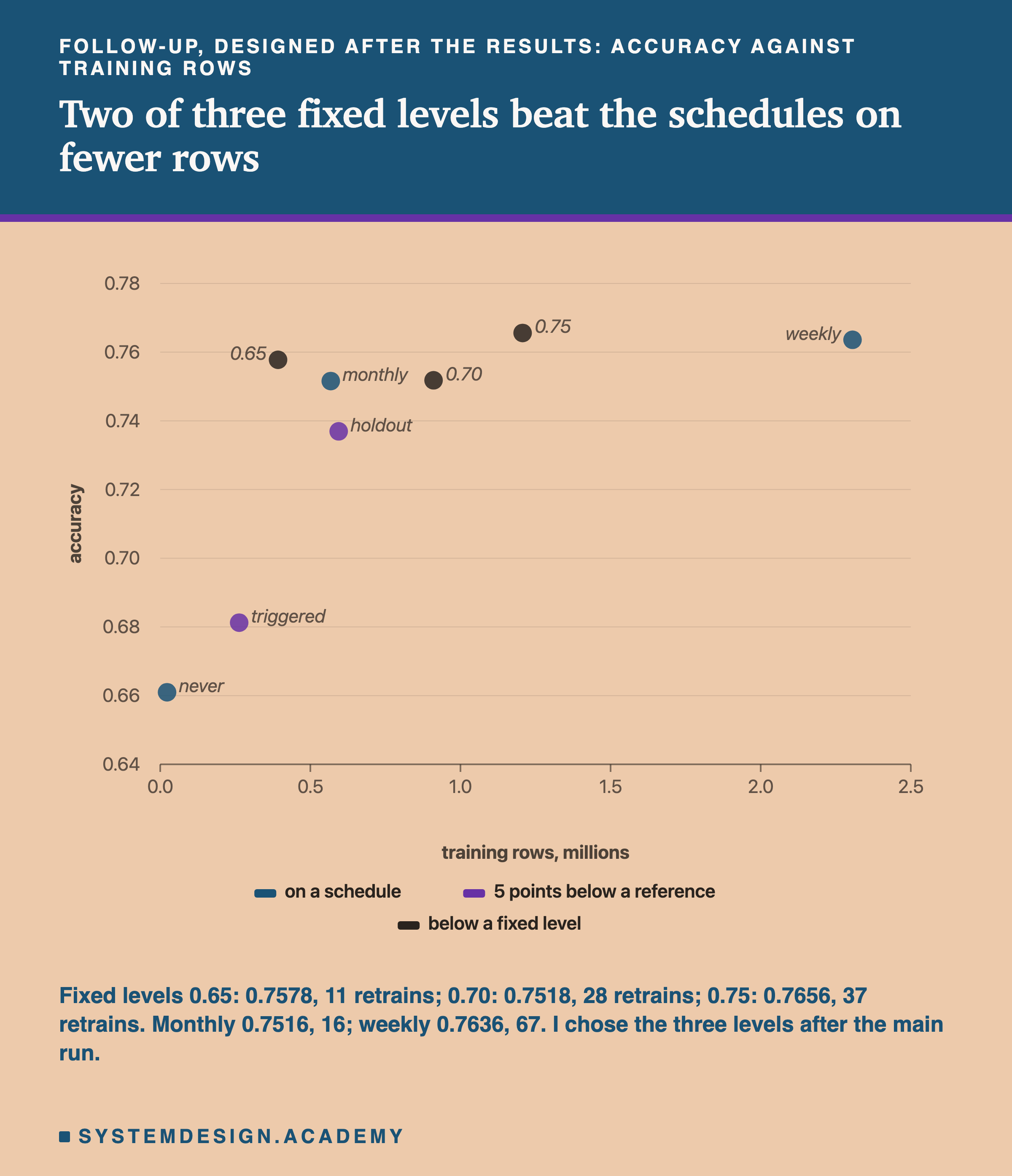
The fixed levels worked much better than the week-after trigger. I call such a fixed level a floor. A floor of 0.65 scored 0.7578 with 11 retrains, above monthly's 0.7516 with 16; a floor of 0.75 scored 0.7656 with 37 retrains, above weekly's 0.7636 with 67; and a floor of 0.70 scored 0.7518 with 28 retrains, level with monthly on 910,416 training rows. Per retrain, the three floors bought 199.4, 73.5 and 64.1 extra correct half-hours, against 128.3 for monthly, and I chose all three levels after seeing the main run, so the best of them flatters itself.
Read this with care. I chose the three levels after I had seen the main run's accuracies, and 0.70 did worse than 0.65 while retraining more than twice as often. If I now told you "use 0.75", I would be picking the best of three on the same data I measured them on, which is the winner's curse from lesson 3. What the follow-up shows is narrower: a bar that does not move with the model avoided the anchoring failure here. It does not show which level is right.
A Reference Set Before Serving Was Anchored Too
The holdout reference seemed like the fix for the anchoring problem. It measures a reference before the model serves anything: a second model, trained without the latest week, is scored on that week. It did better than the week-after trigger, but not as well as the fixed floors.
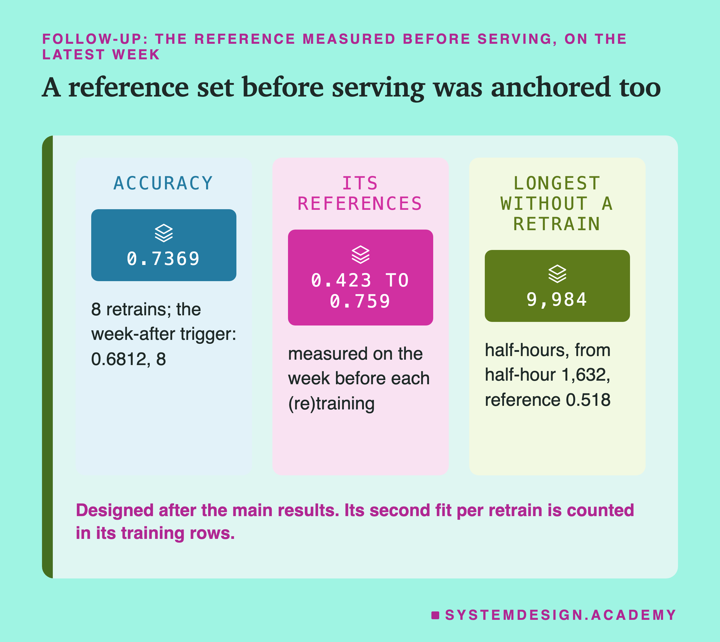
It scored 0.7369 with 8 retrains, against 0.6812 for the week-after trigger with the same number of retrains. But its references ranged from 0.423 to 0.759. After a retrain at half-hour 1,632, its reference was 0.518, so its bar was about 0.47, and it went 9,984 half-hours, more than 200 days, without firing. The same problem again: when the week used as the reference is a bad week, the bar is low, and a low bar lets a weak model run.
So the problem is not only when the reference is measured. It is that the reference is one week of results from the model or its near twin. Any bar built that way inherits that week's bad luck. A fixed level is a statement about what the business needs, and it does not move when the model has a bad week. That is my reading of these two results; one run each.
What the Frozen Model Was Really Missing
Back to the question from the first slides: why did the frozen model start saying UP on nearly every half-hour? The bikes lesson had found that retraining helped only through the year input. Elec2 has a similar input, date, a number that mostly grows as time passes (lesson 1 found it steps backwards 5 times). So the follow-up also ran never, monthly and weekly with the date set to 0 on every row, so that no tree could use it.
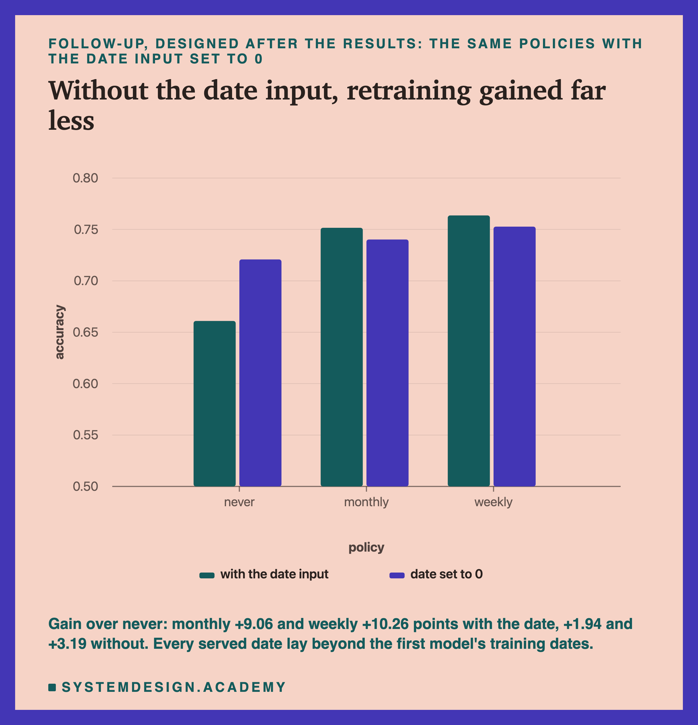
Without the date, the frozen model scored 0.7208 instead of 0.6610. It was 6 points better by knowing less. And it did not decay over the run: 0.679 in the first block and 0.810 in the last. Monthly without the date scored 0.7402 and weekly 0.7527, so retraining still helped, but by 1.94 and 3.19 points instead of 9.06 and 10.26.
Here is what I measured about why, after the results. Every one of the 22,656 served half-hours had a date larger than any date the first model had learned from. I asked the first model again, with every served date replaced by the last date in its training rows, and it gave the same answer on 100.0% of rows. So the frozen model treated every served half-hour, for 16 months, as if it were the last day of its training. Trees split an input into ranges they saw in training, and a value past the largest range falls into the last one; the 100.0% confirms that here. Removing the date changed 26.7% of the frozen model's answers.
The date is not the whole story, though. The frozen model trained without the date also over-called UP in blocks 12 to 14: 0.722, 0.817 and 0.688 of half-hours, against a truth of 0.402, 0.555 and 0.533; with the date it was 0.891 to 0.958. In the first eleven blocks it went the other way, saying UP on only 0.054 to 0.331 of half-hours. So the date made the surge much worse, but something else pushed the same way in those months. That fits lesson 1's guess about July 1998, that the trees read a high price level as UP; I did not test it here either. Why the last days of training, in August 1997, pushed the trees towards UP is also a guess.
The Bikes Lesson, Compared Honestly
This finding sits next to the bikes lesson, and the two are not the same, so here they are side by side.
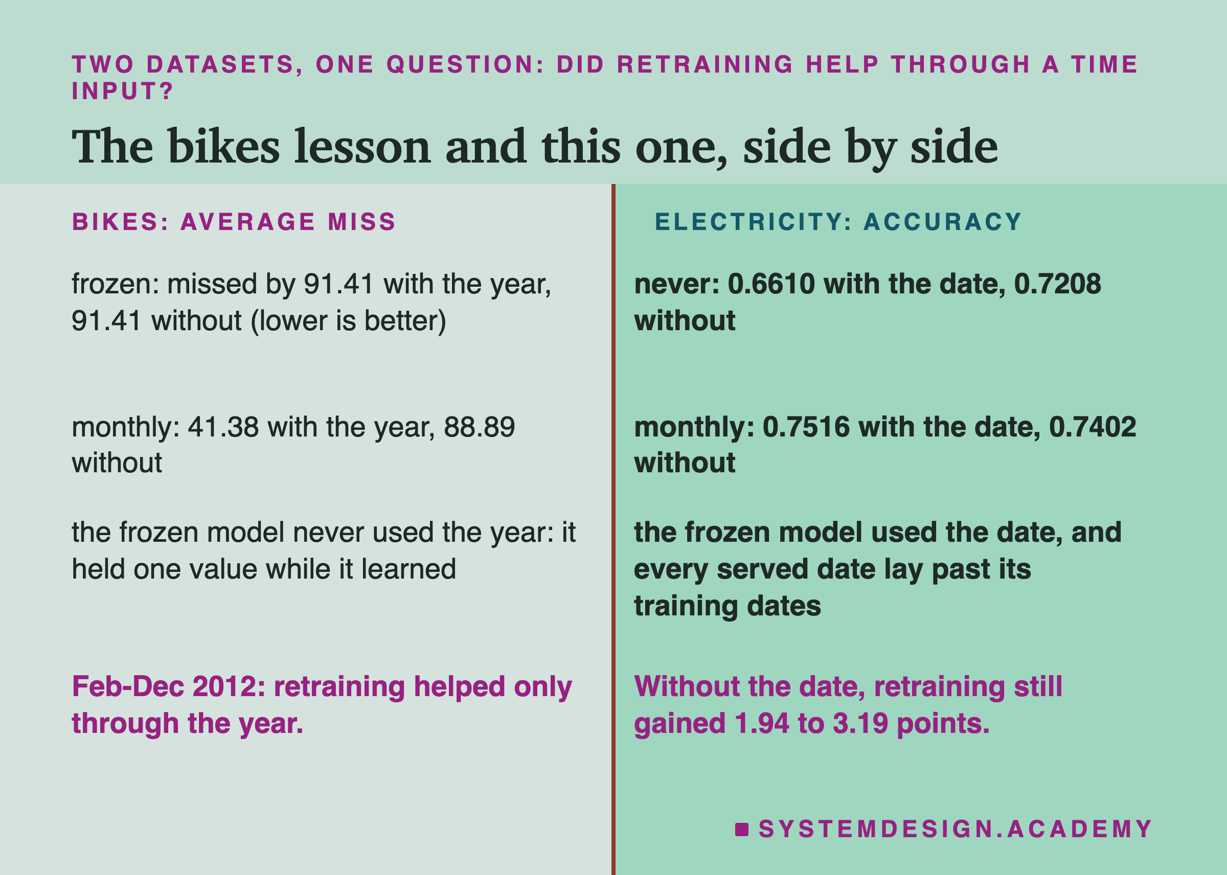
In the bikes lesson, the frozen model had learned from one year only, so its year input held one value and it could never use it. Retraining brought in rows from the new year, the year input started to mean something, and that is how retraining helped. Without the year, monthly retraining missed by 88.89 bikes an hour, barely better than the frozen 91.41.
Here, the frozen model could use the date, because its training rows spanned 15 months, and the date hurt it once the served dates ran past anything it had seen. My interpretation: retraining helped mostly by moving the model's idea of "latest" forward, which repaired that damage. Without the date, retraining still helped a little, 1.94 points for monthly and 3.19 for weekly, which is a real if modest gain from fresh rows.
In both datasets, a single input about when decided how much retraining appeared to help. Here, most of retraining's value was repairing the date input. Before you measure the value of retraining, find the inputs that only say when, and check what your model does with them once time moves past its training.
The Reminder from Lesson 1
Every number in this lesson so far compares trained models with each other. Lesson 1 set a harder bar: a model must beat the best rule that learns nothing.
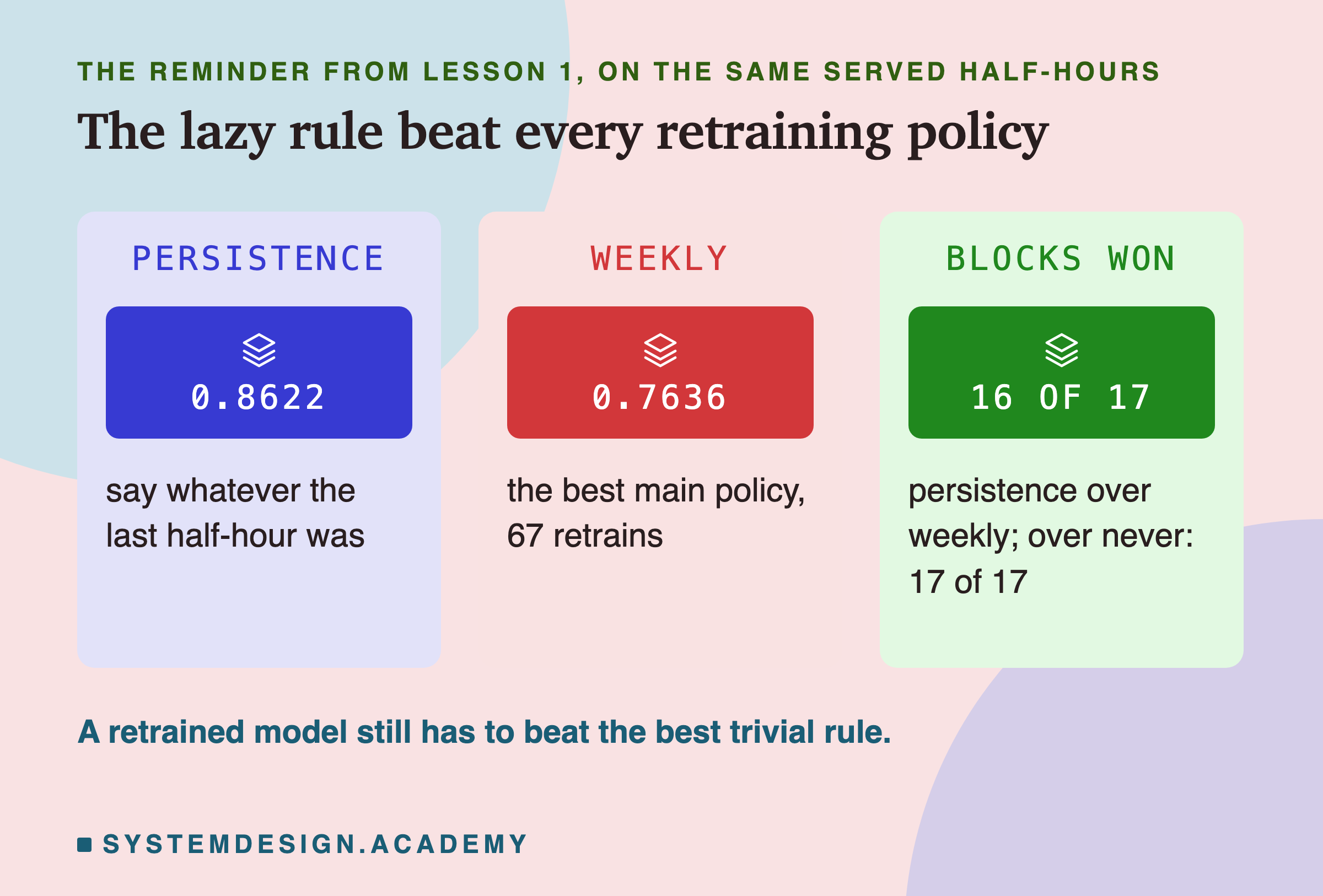
Persistence scored 0.8622 on the same 22,656 half-hours. The best policy of the main run, weekly, scored 0.7636, and the best of the follow-up, the 0.75 floor, scored 0.7656. Persistence won 16 of 17 blocks against weekly and all 17 against never. Retraining did not change the ranking.
So the most useful change to this model was never going to be its retraining policy. Lesson 1 showed that giving the trees the previous half-hour's label as an input closed most of the gap, and that on this data the honest answer may be to ship persistence. A retraining policy can keep a model from getting worse; it cannot make a weak framing, the choice of what the model predicts and from which inputs, strong. Check the baseline first, and only then tune how often to retrain.
The Answers Arrived Half an Hour Later
Every result here assumed that the right answer arrives half an hour after the guess. That is what makes a trigger possible at all: the rolling window can be measured every day. Many real systems are not like that. Whether a loan is repaid is known months later; a fraud report can come weeks after the payment.
This lab's weekly run was also the first run of a label-delay lab, so I checked the two against each other. The delay lab's weekly run with labels arriving after one half-hour scored 0.7636, the same as weekly here, in every block. The label delay is how long the right answer takes to arrive. With later labels, the same weekly schedule could only retrain on rows whose answers had arrived: a day late, 0.7563; a week late, 0.7299; four weeks, 0.7315, slightly above one week, so the fall is not smooth; twelve weeks, 0.6954.
A schedule also loses value when labels are late: 0.7636 to 0.6954 here. A trigger is hurt twice, since its window is late too: by the time it sees a bad week, the model has already served that week and more. That comparison is my reasoning, not a measurement; I did not run a trigger with late labels. A later lesson in this chapter measures label delay in detail.
What I Would Do Instead
Here is what the lab points to, in the order a team meets it.
Measure how fast your model goes stale. Keep a frozen copy of the model running on recent labelled rows, and score it block by block. Here the frozen model looked fine for ten months and then collapsed. Without that measurement, any retraining policy is a guess.
Find the inputs that only say when. A date, a counter, a version number, a week index. Check what the model does when their values go past the training range. Here the date input cost the frozen model 6 points, and made retraining look several times more valuable than it was: +9.06 points for monthly with the date, +1.94 without.
Start with a schedule you can afford. A schedule is predictable and easy to review, and it can run before any label has arrived, though late labels make each retrain worth less (0.7636 to 0.6954 here). Here 16 monthly retrains bought 9.06 points; the next 51 bought 1.20 more.
If you add a trigger, give it a fixed floor. Decide in advance what accuracy you need, before you look at the results, and retrain when the rolling window falls below it. Never measure "worse" only against the model's own first week: here that bar fell to 0.405 and let a weak model serve half the run.
Count the cost of each retrain. Training rows, compute, the reviewer's time, and the risk that the new model is worse. Here a retrain made a month worse than never in 5 of 17 blocks.
Put every retrain through the gate. Lesson 4's gate and lesson 5's shadow exist for this: a retrained model is a new model, and it must show it is better before it replaces the old one.
Try It Yourself
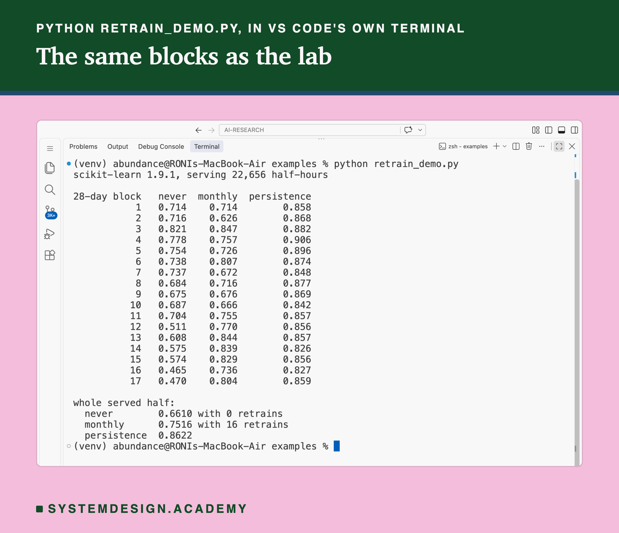
This script is the lab made small. It downloads the same data, trains the same trees on the first half, and serves the second half twice: once never retraining, and once retraining every 28 days on all rows seen so far. It prints the accuracy of both and of persistence in each block of 28 days, and the totals. It does not need a GPU, the graphics chip large models train on.
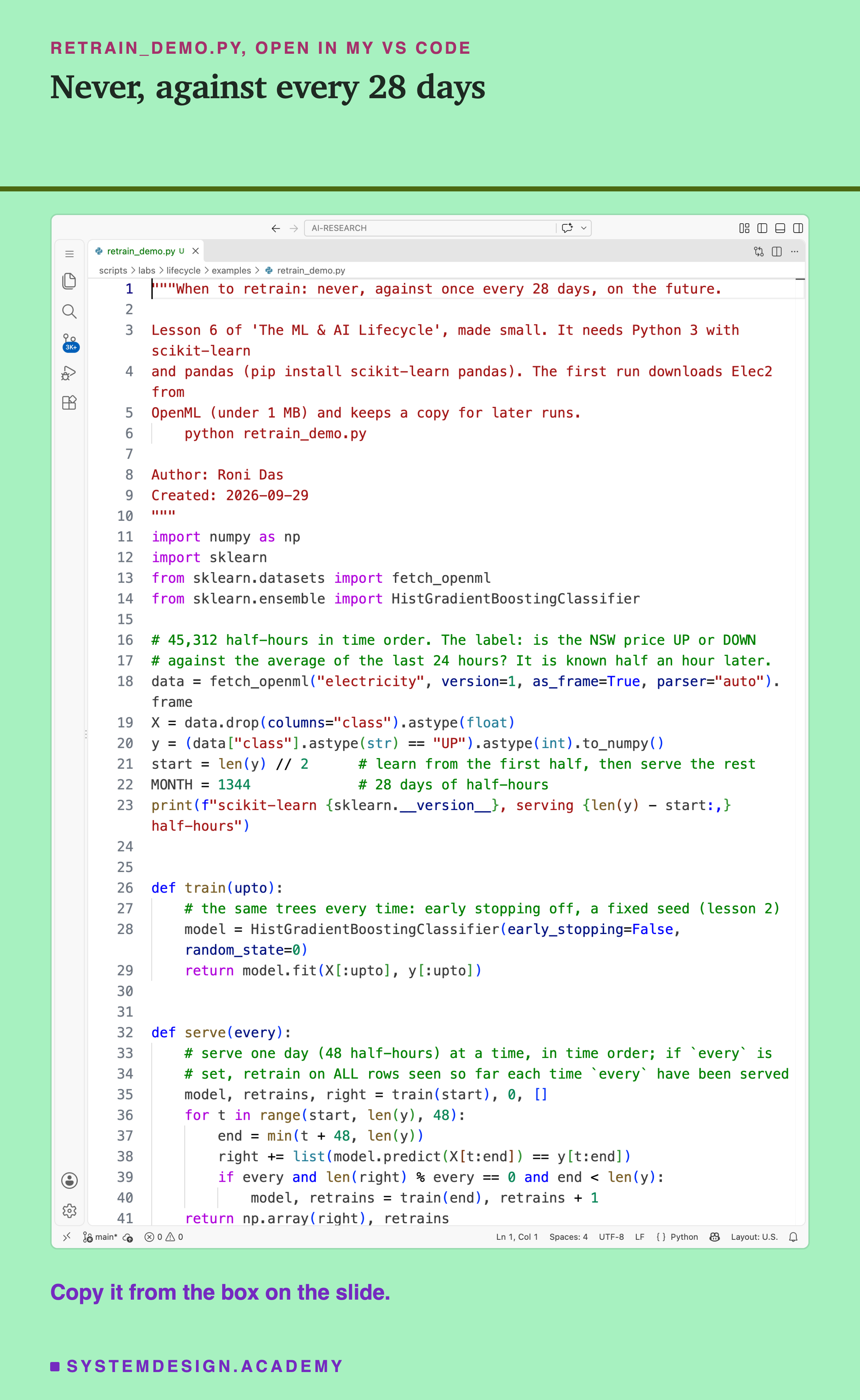
Before you run this lab. You need Python 3 and two libraries: pip install scikit-learn pandas. scikit-learn holds the model and the download, and brings NumPy with it; pandas holds the table. The first run downloads Elec2 from OpenML (under 1 MB compressed), so it needs an internet connection once; scikit-learn keeps a copy in a folder in your home directory (scikit_learn_data) for later runs. It fits 18 small models (one for never, one plus 16 retrains for monthly); I did not time it. I ran it with scikit-learn 1.9.1 on a Mac. scikit-learn runs the same way on Windows and Linux, but I have not checked the numbers there, and another version of scikit-learn may give different decimals, which is why the first line printed is the version.
"""When to retrain: never, against once every 28 days, on the future.

Lesson 6 of 'The ML & AI Lifecycle', made small. It needs Python 3 with scikit-learn
and pandas (pip install scikit-learn pandas). The first run downloads Elec2 from
OpenML (under 1 MB) and keeps a copy for later runs.
    python retrain_demo.py

Author: Roni Das
Created: 2026-09-29
"""
import numpy as np
import sklearn
from sklearn.datasets import fetch_openml
from sklearn.ensemble import HistGradientBoostingClassifier

# 45,312 half-hours in time order. The label: is the NSW price UP or DOWN
# against the average of the last 24 hours? It is known half an hour later.
data = fetch_openml("electricity", version=1, as_frame=True, parser="auto").frame
X = data.drop(columns="class").astype(float)
y = (data["class"].astype(str) == "UP").astype(int).to_numpy()
start = len(y) // 2      # learn from the first half, then serve the rest
MONTH = 1344             # 28 days of half-hours
print(f"scikit-learn {sklearn.__version__}, serving {len(y) - start:,} half-hours")


def train(upto):
    # the same trees every time: early stopping off, a fixed seed (lesson 2)
    model = HistGradientBoostingClassifier(early_stopping=False, random_state=0)
    return model.fit(X[:upto], y[:upto])


def serve(every):
    # serve one day (48 half-hours) at a time, in time order; if `every` is
    # set, retrain on ALL rows seen so far each time `every` have been served
    model, retrains, right = train(start), 0, []
    for t in range(start, len(y), 48):
        end = min(t + 48, len(y))
        right += list(model.predict(X[t:end]) == y[t:end])
        if every and len(right) % every == 0 and end < len(y):
            model, retrains = train(end), retrains + 1
    return np.array(right), retrains


never, _ = serve(None)
monthly, retrains = serve(MONTH)
persist = y[start - 1:-1] == y[start:]   # say what the last half-hour was

print("\n28-day block   never  monthly  persistence")
for b in range(0, len(never), MONTH):
    cells = [x[b:b + MONTH].mean() for x in (never, monthly, persist)]
    print(f"{b // MONTH + 1:>12}   {cells[0]:.3f}    {cells[1]:.3f}        {cells[2]:.3f}")

print("\nwhole served half:")
print(f"  never        {never.mean():.4f} with 0 retrains")
print(f"  monthly      {monthly.mean():.4f} with {retrains} retrains")
print(f"  persistence  {persist.mean():.4f}")
The Lab Report
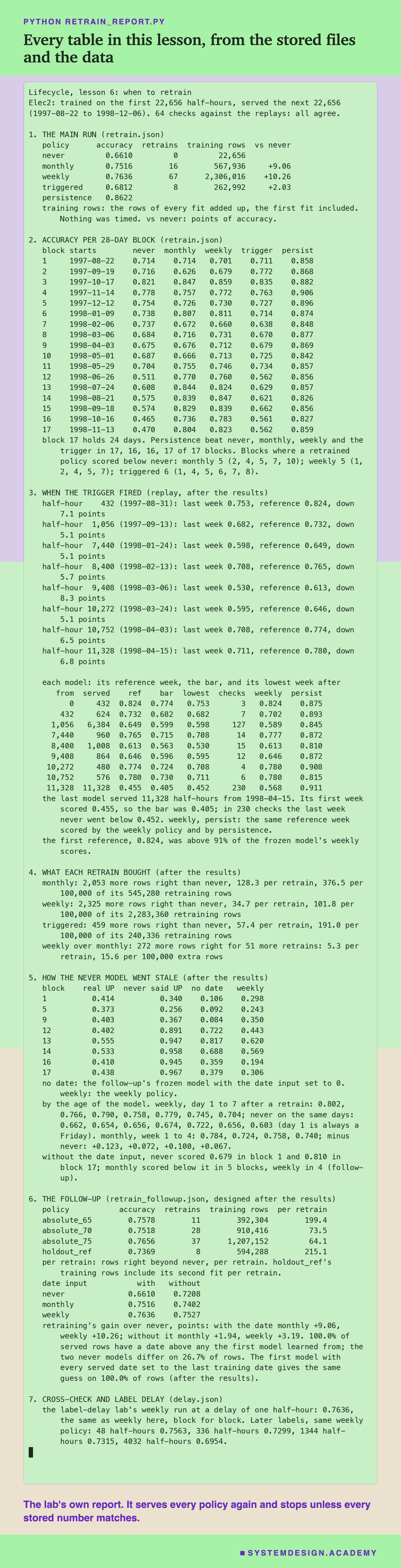
The report lives in scripts/labs/lifecycle/retrain_report.py. It reads the lab's stored files, results/retrain.json and results/retrain_followup.json, the label-delay lab's results/delay.json, and the Elec2 data from scikit-learn's local copy. The lab stored accuracies, retrain counts and training rows, not each answer or when the trigger fired. So the report serves every policy again, main and follow-up, using the lab's own training function, in a copy of the lab's serving loop that also writes down every check. It stops unless every stored accuracy, block accuracy, retrain count and training-row total comes back unchanged. It makes 64 checks in all, and they all agree. It changes nothing in the lab's files.
Its json mode writes every number to results/rr-report.json, which the figures read. The demo mode checks the student script's stored run, and the mode writes the playground below and checks that it gives the lab's accuracies and the lab's first trigger firing.
Design a Trigger Yourself
This box has no model in it. It holds the real right-or-wrong outcome of the four main policies on all 22,656 served half-hours, one hexadecimal digit per half-hour (counting in sixteens, with the digits 0 to 9 and a to f), and the real labels, four to a digit. The report checked that every accuracy and block it prints matches retrain.json. It runs in your browser.
As it is, the box prints each policy's accuracy, retrains, training rows and correct answers per retrain beyond never, then persistence, then the frozen model and the weekly policy block by block.
Now design a trigger. first_fire('never', drop=0.05) asks when a trigger that compares the last 7 days with the first 7 days would first fire on the frozen model: it returns half-hour 432, where the lab's trigger first fired, because until its first retrain the triggered policy is the frozen model. first_fire('never', level=0.65) uses a fixed floor instead and returns 1,296, where the follow-up's 0.65 floor first fired. Try first_fire('triggered', level=0.6) to see how soon a floor would have caught the triggered policy, and first_fire('never', window=1344, drop=0.05) for a 28-day window. The box can only tell you when a rule would first fire, not what a retrained model would have done afterwards; that needs the real lab.
The Code, Part by Part
Loading. fetch_openml("electricity", version=1) downloads Elec2 once and reads the local copy after that. The label column holds the words UP and DOWN, turned into 1 and 0. start = len(y) // 2 is 22,656: the model learns from the rows before it and answers the rows after it.
train. Builds a fresh HistGradientBoostingClassifier with early_stopping=False and random_state=0 and fits it on the first upto rows. Lesson 2 found that with early stopping off, the seed changes nothing here, so the same rows always give the same model. That is what makes the demo land on the lab's numbers.
serve. Walks through the served rows one day, 48 half-hours, at a time. The model answers the day, and each answer is marked right or wrong against the real label. If every is set and a multiple of every half-hours has been served, the model is trained again on every row up to now. serve(None) never retrains. serve(MONTH) retrains every 1,344 half-hours, 16 times in all, so the script fits 18 models.
Persistence. y[start - 1:-1] == y[start:] pairs each served label with the one before it: right only when the label did not change.
How to Set a Retraining Policy
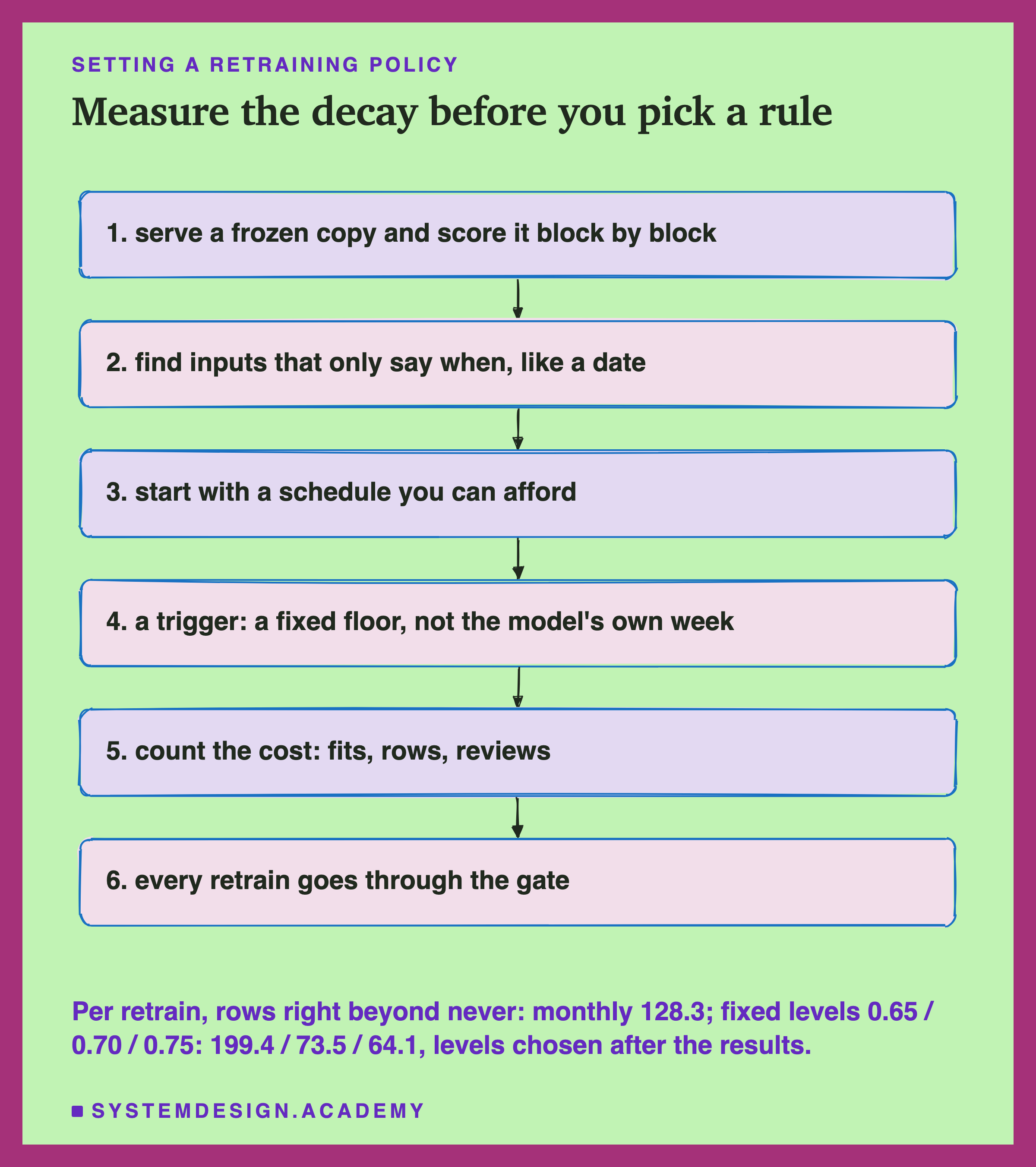
Serve a frozen copy. Keep the current model's answers on recent labelled rows, and score them in blocks of a week or a month. That curve is the decay you are trying to prevent, and it tells you how fast it happens.
Find the time inputs. List every input that grows with time, or names a period. For each, check the range it had in training and the range it has now. If the new values are past the old ones, test the model with that input fixed, as the follow-up did.
Start with a schedule. Pick the longest interval whose decay you can live with, from the frozen copy's curve. Write it into the pipeline's configuration.
Add a fixed floor if you need one. Decide the level before you look, from what the business needs, not from the model's recent history. Retrain when the rolling window falls below it, and keep a minimum gap between retrains.
Count the cost. Log every retrain with its training rows, its time and what it gained. If the gains per retrain shrink towards nothing, retrain less often.
Gate every retrain. Score each new model against the live one before it takes over.
A Schedule or a Trigger, When?
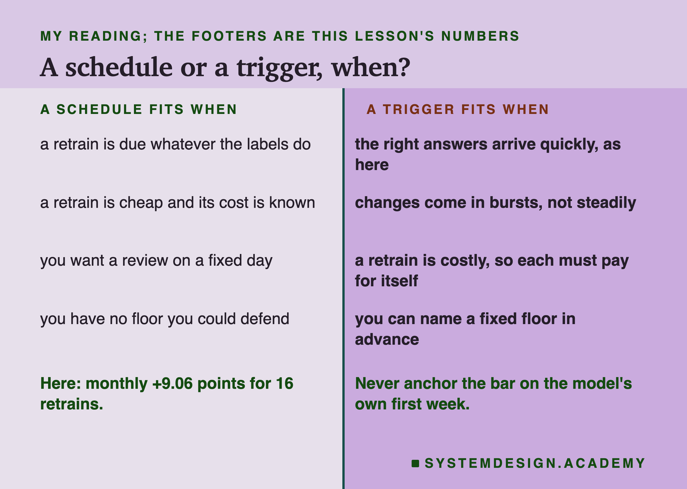
Think about a schedule when labels are late. A trigger can only react to answers it has, so with labels that take weeks it is always behind. A schedule suffers too (0.7636 to 0.6954 here at a 12-week delay); it at least retrains on time. That is reasoning; I did not measure a late-label trigger.
Use a schedule when a retrain is cheap and you want predictability. Here 16 monthly retrains of small trees bought 9.06 points; I did not time them. A fixed day also makes it easy for someone to review each new model.
Use a trigger when labels arrive fast and a retrain is expensive. Then each retrain must pay for itself, and a trigger skips the ones that would buy nothing. Here the three floors bought 199.4, 73.5 and 64.1 correct answers per retrain, against 128.3 for monthly, with levels I chose after the results.
Use a trigger when changes come in bursts. A schedule cannot know that the market changed yesterday; a floor sees it within a window.
Do not use a trigger that compares the model only with itself. Here that bar fell to 0.405 and let a weak model serve half the run.
Do not retrain more often just because you can. Here the step from monthly to weekly bought 5.3 correct answers per extra retrain.
What These Numbers Can and Cannot Tell You
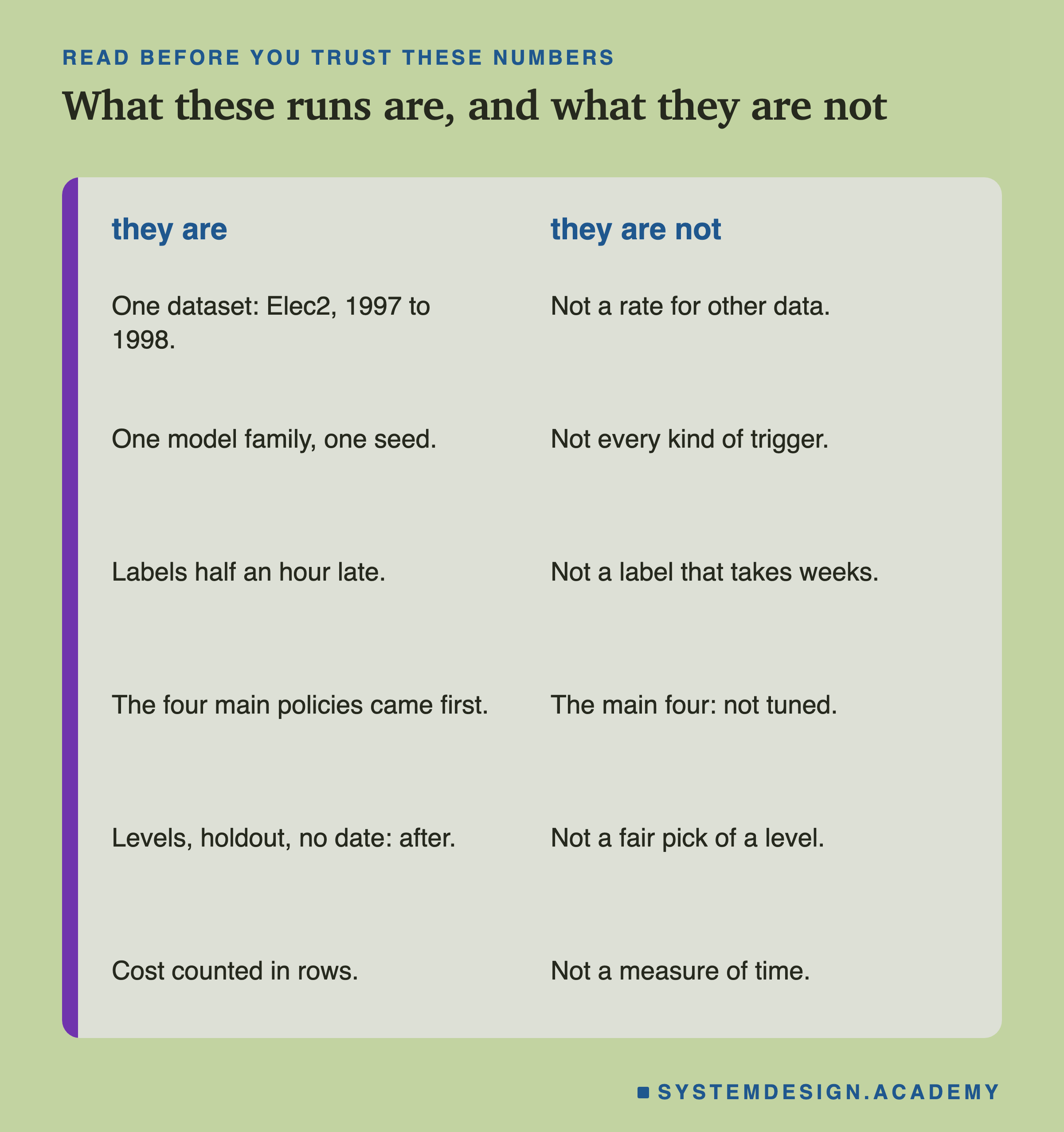
One dataset, one model family, one run each. Everything here is boosted trees on 16 months of one electricity market. With other data, other decay and other inputs, the numbers would move. Each policy ran once, and no significance test was declared, so I do not call any gap significant.
One trigger design in the main run. The week-after trigger failed here for a reason I could see. That is a result about this design, not about triggers in general: the fixed floors in the follow-up did well. I did not test triggers on input drift, which the pipelines lesson calls the strongest kind, because measuring drift is a subject of its own.
The follow-up came after. The fixed levels, the holdout reference and the runs without the date were designed after I saw the main results and written down before they ran. I chose the three levels knowing the main run's accuracies, and picking the best of them would flatter it.
After the results. When the trigger fired, each model's reference, the gain per retrain, the share called UP, the accuracy by age and the date check were all measured after the results. Why the trees said UP so often in the last months is a guess.
Cost in rows, not time. Nothing was timed. On a larger model the cost of a retrain would be very different, and so would the best policy.
What to Do Next
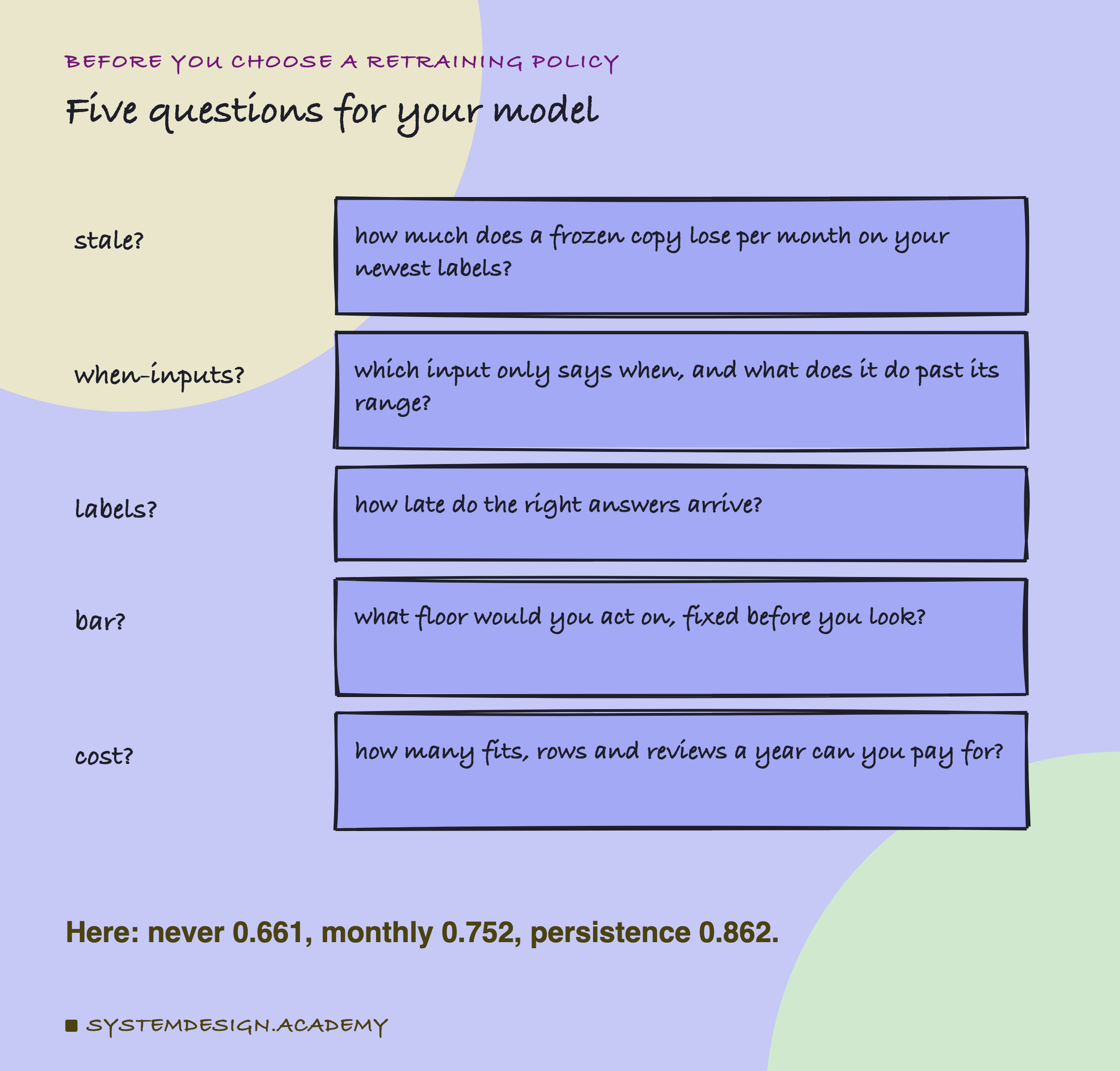
Take the model your team retrains most often, and ask the five questions on the card. If nobody knows how much a frozen copy loses per month, start there: it is one model you already have, scored on labels you already collect.
Then look at your trigger, if you have one. Write down exactly what it compares with. If the answer is "the model's accuracy just after it went live" or "last week's accuracy", check what happens after a retrain that starts badly. Replace it with a floor written down before anyone looks, and log every firing with its window and its reference.
The next lesson planned for this chapter looks at stale pieces inside a pipeline: a cached input or an old saved file that the model keeps using without anyone noticing, and what that silently does to its answers.
Knowledge Check
Knowledge Check
4 questions - Score 80% to pass
The triggered policy compared each week with the model's own first week and went 11,328 half-hours without a retrain. What was the measured reason?
Weekly retraining scored 0.7636 with 67 retrains, monthly 0.7516 with 16. What did each extra retrain of weekly buy over monthly?
With the date input set to 0, the frozen model scored 0.7208 instead of 0.6610. What did the report find about the date?
Weekly accuracy was 0.802 on day 1 after a retrain and 0.704 on day 7. Why is that not proof that the model decayed within the week?