Let me start with a jar.

Imagine a friend asks you the same hard question every few minutes. The first time, you think hard and work out the answer. Then you write it on a small ball and drop it in a jar. The next time the question comes, you just take the ball out. That is much faster than thinking again.

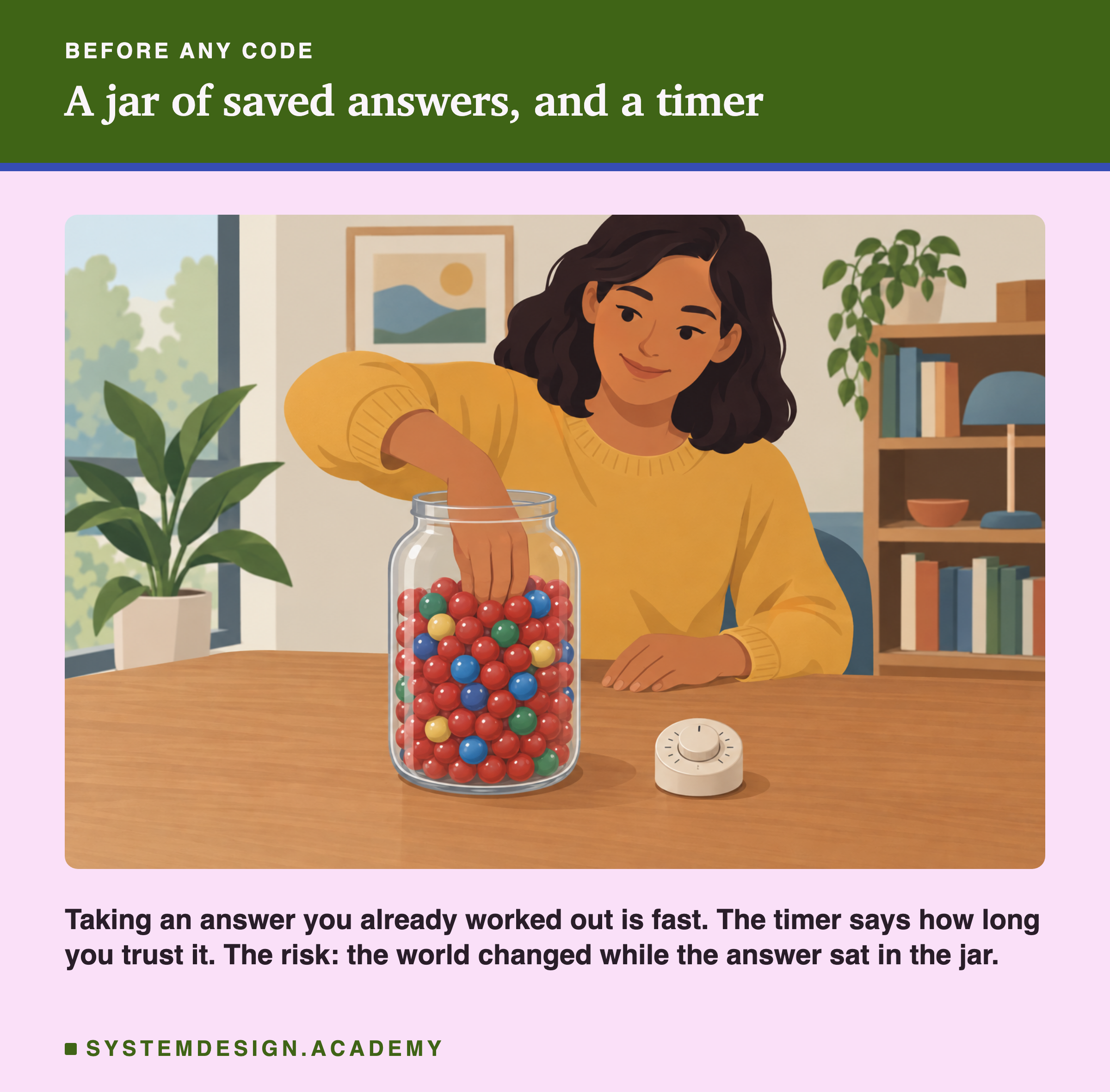
There is a timer next to the jar. You set it when you drop a ball in. When the timer rings, you throw that ball away and think again next time. The timer is how long you trust an old answer.

The jar has one danger. Your answer was right when you wrote it. But maybe something happened since then that changes the answer, and the ball in the jar does not know it.

A model that gives scores can have a jar too. In this lesson I fill one with real requests and measure how often it helps and how often it serves an answer that is out of date.

This is lesson 8 of the chapter on serving a model. The model is the one from lesson 1, batch or online. It reads six numbers about a customer of a real UK gift shop. Then it gives a score: how likely the customer is to buy again in the next 30 days.

Lesson 1 asked a close question. It compared a score made at the moment of a visit with a score made earlier by a nightly, weekly or monthly batch. On this shop, even a score 30.7 days old could not be told apart from a fresh one. A cache is a different machine with a similar risk. A batch scores everyone on a schedule. A cache scores a customer only when they ask, keeps that answer, and gives it out again later. So I wanted to know: does lesson 1's result hold for a cache, and what extra choices does a cache add?

The course has a lesson on caching for retrieval and language models. That one is a semantic cache: it matches two questions that mean the same thing, even when the words differ. This lesson is about something simpler and more common for small models: an exact-key cache, where a hit needs the same key, letter for letter. I do not repeat that lesson here.

Please read this slide slowly if any word is new. Every slide after it uses these words.

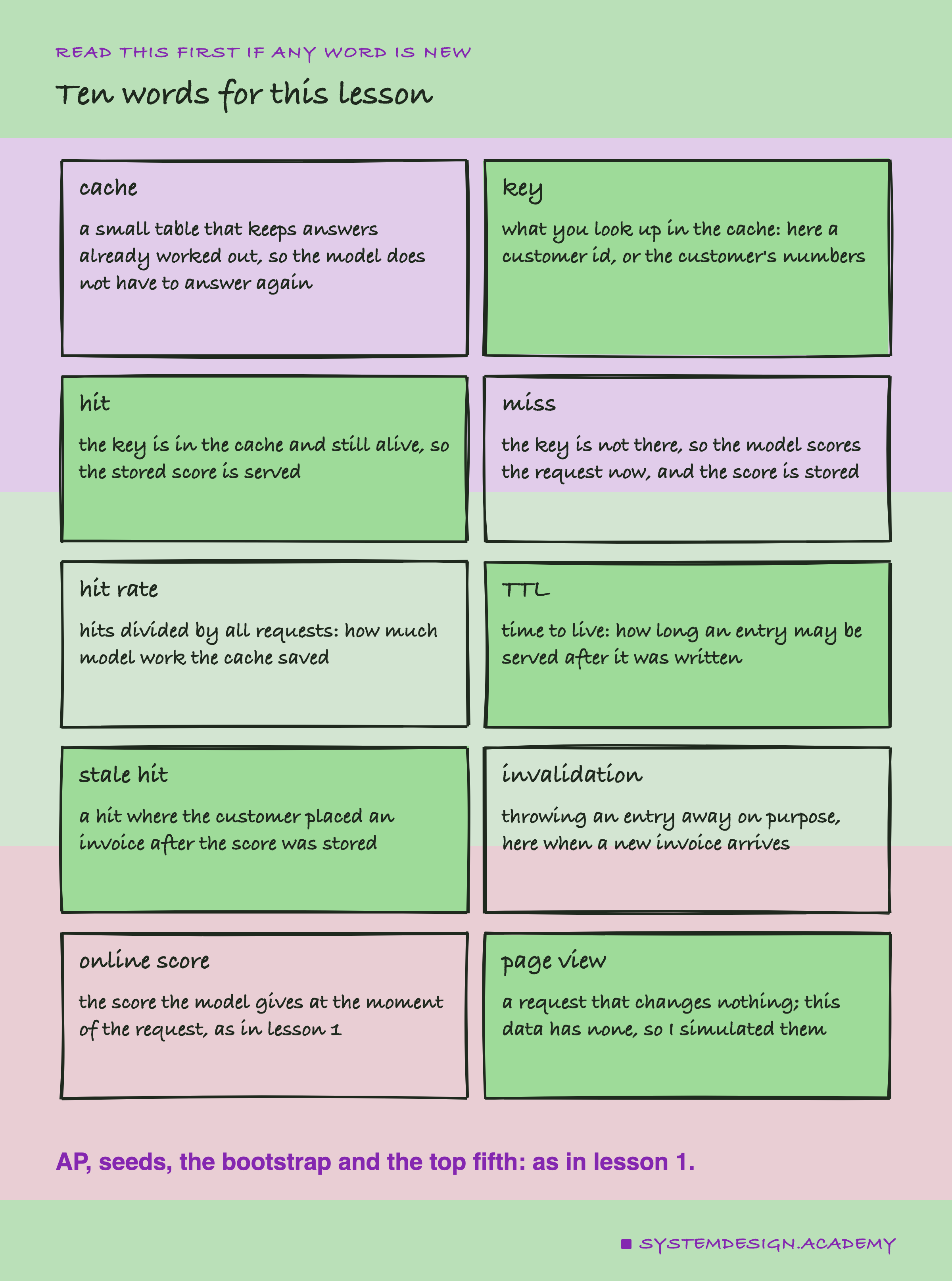
A cache is the jar: a small table that keeps answers. Each answer is stored under a key, the thing you look up. If the key is there and still alive, that is a hit, and the stored score is given out. If it is not there, that is a miss: the model scores the request now, and the new score goes into the cache.

The hit rate is the share of requests that were hits. It tells you how much model work the cache saved.

The TTL, time to live, is the timer. It is how long an entry may be served after it was written. In this lab, reading an entry does not restart its timer. In Redis, a plain read does not change a key's timeout either; a new EXPIRE (or GETEX with an expiry option) does.

A stale hit is a hit where the customer placed an invoice after their score was stored, so the stored score never saw that invoice. Invalidation means throwing an entry away on purpose before its timer ends. Here I throw it away when a new invoice arrives.

Here is what happens to one request when a cache sits in front of the model.

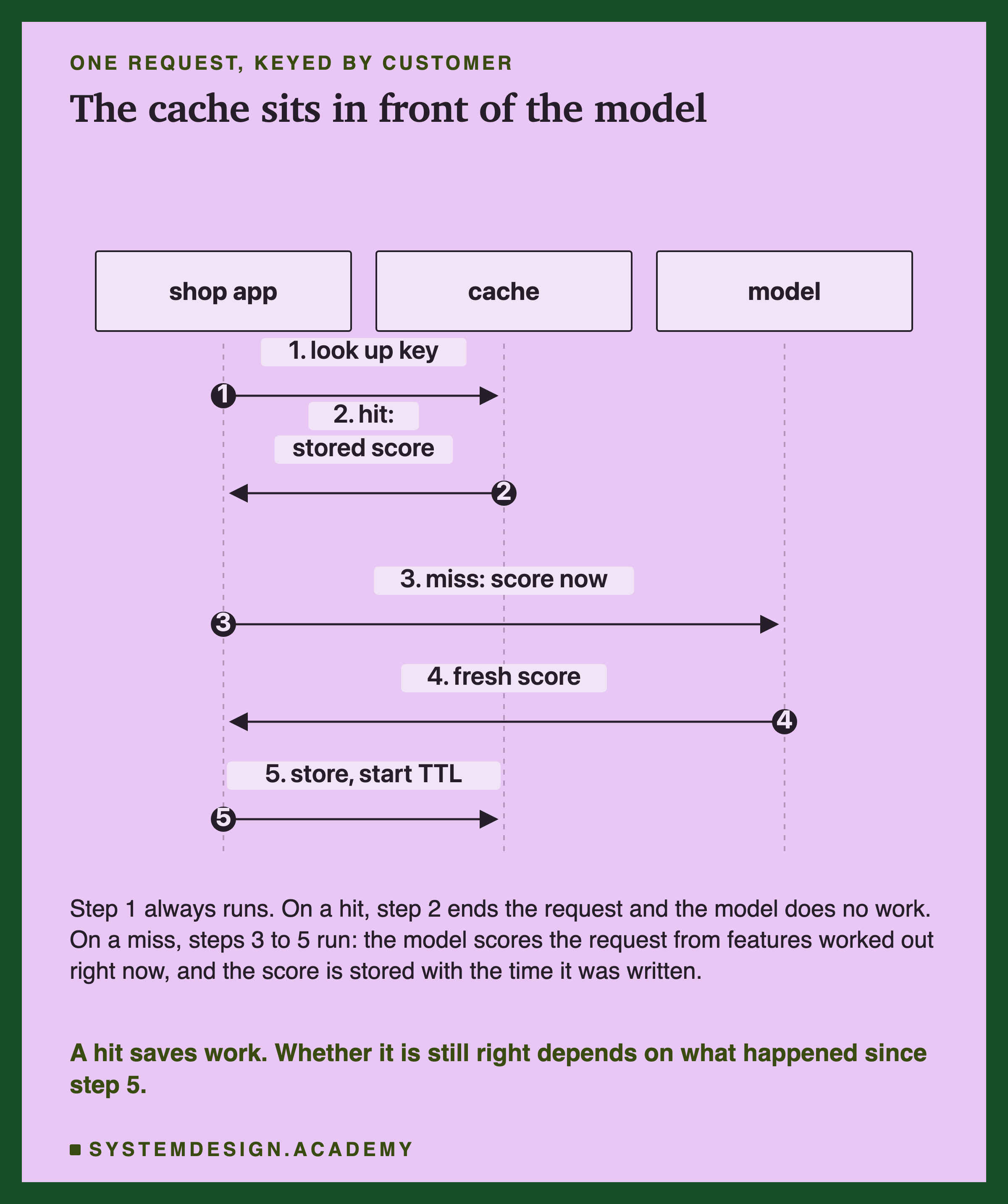
The app first looks up the key. On a hit, it gets a stored score and stops there. The model does nothing.

On a miss, the app works out the customer's six numbers as they are right now and asks the model. This is the online score from lesson 1. Then the app stores that score in the cache, with the time it was written. From that moment, the TTL timer runs.

Why bother? Every miss runs the model, and lesson 2 of this chapter measured that a single prediction was the biggest part of one request's time on a quiet machine. A cache skips that work on every hit. For a small model like this one the saving per request is small. For a large model, or a model that needs slow feature lookups, it can be most of the cost.

So every hit gives the score from some earlier miss. The questions of this lesson are about that gap. How often is there an earlier miss close enough to serve? And did anything happen in between that the stored score does not know?

This lesson leans on what three caches and one library promise. I downloaded each source at a fixed version and found every quote in it word for word. The lab's fact-check mode wrote them to results/pc-factcheck.json.

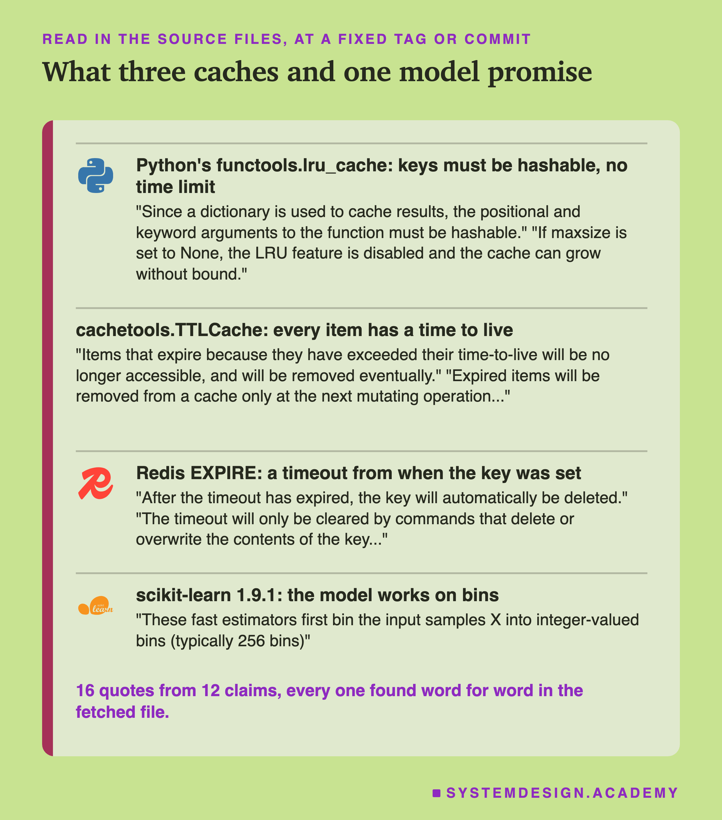
Python's functools.lru_cache is the cache most people try first. It keys on the function's arguments, and those must be hashable, which a numpy row is not. And it has a size limit but no time limit at all. Put it on a function that takes a customer id, and a score stays in it until it is pushed out by size, however old it is.

cachetools.TTLCache gives every item a time to live. Expired items are no longer served, but they may "still claim memory" until the next change to the cache.

Redis is a separate server that many teams use as a shared cache. Its EXPIRE command deletes a key after a timeout. Commands that change a value without replacing the key "will leave the timeout untouched", so a plain GET does not change it. Calling EXPIRE again sets a new time to live, and can read a key and set its expiration in one step. The cachetools documentation says the same for its own cache: the expiry time is fixed "at the time of insertion". The same page says Redis removes expired keys when someone reads them, and also by testing a few keys at random now and then.

I wrote the lab's design into the docstring of scripts/labs/serving/caching_predictions.py before it first ran. Before that, I had read lesson 1's code and results and the three cache documents. I had not replayed any cache or counted any repeat request.

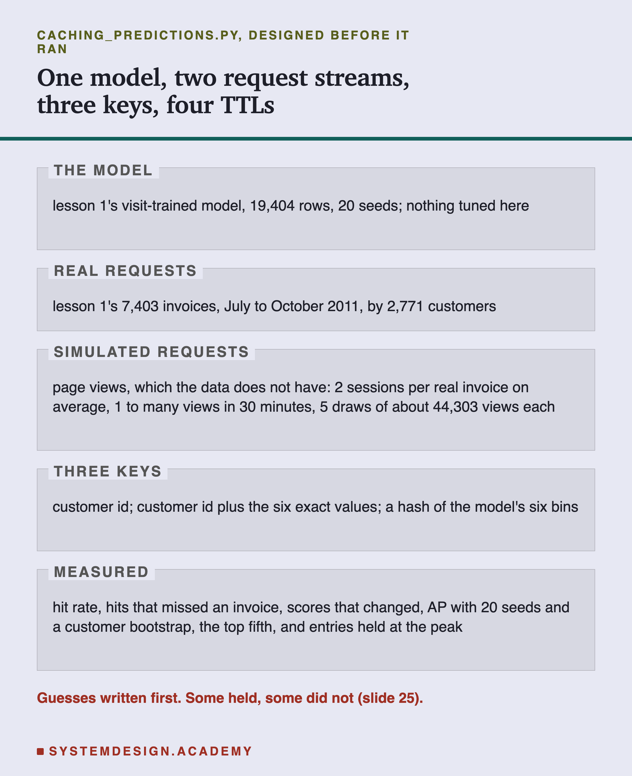
The model. I used lesson 1's second model, the one trained on 19,404 rows made at the moment of real visits. Lesson 1's review showed it fits visit-time requests better than the first model. The lab trains it 20 times, with seeds 0 to 19. It stops unless every seed gives exactly the empty-row score and the online AP that lesson 1 stored.

Three keys. A cache is defined by its key, so I tried three. Key one is the customer id alone. Key two is the customer id plus the exact six numbers at the request. Key three is a short hash of the model's six bins, with no customer id. A hash is a short code made from some data: the same data always gives the same code.

Four TTLs. 1 hour, 1 day, 7 days and 30 days. For the customer key I also tried invalidation: when a new invoice from that customer arrives, their entry is dropped.

A cache only helps when the same key comes back. So the most important input is the stream of requests.

The real stream is lesson 1's 7,403 invoices from July to October 2011. Each invoice is a moment the shop wanted a score.

But here is a fact I wrote down before the run.

In this data, every request is an invoice, and an invoice is exactly the event that changes a customer's six numbers. A customer-keyed entry is written at one invoice, from the numbers just before that invoice. So when the customer comes back, the entry has always missed at least one invoice: the one that wrote it. Every hit on the real stream must be stale. And dropping the entry on each invoice must turn every hit into a miss. Both are true by construction, which means the design makes them true, not the data. The lab counts them anyway, and I will not treat them as findings.

The simulated stream fixes that. A real shop also scores page views: a customer looks at products, and the page shows offers based on their score. A page view changes none of the six numbers. This data has no page views, so I made them up, on the real customers.

Every customer gets on average 2 browsing sessions per real invoice, at random moments in the four months. Each session has 1 view plus a random number more, 2 on average, all within 30 minutes. I drew this five times, with five different random seeds. Every result from this stream is labelled SIMULATED. The parameters are my assumption, not a measurement.

How sure. For AP I used lesson 1's method: 20 seeds, and a bootstrap that redraws the customers 1,000 times within each month. If the middle 95% of the differences crosses zero, the cache "cannot be told apart" from online scoring.

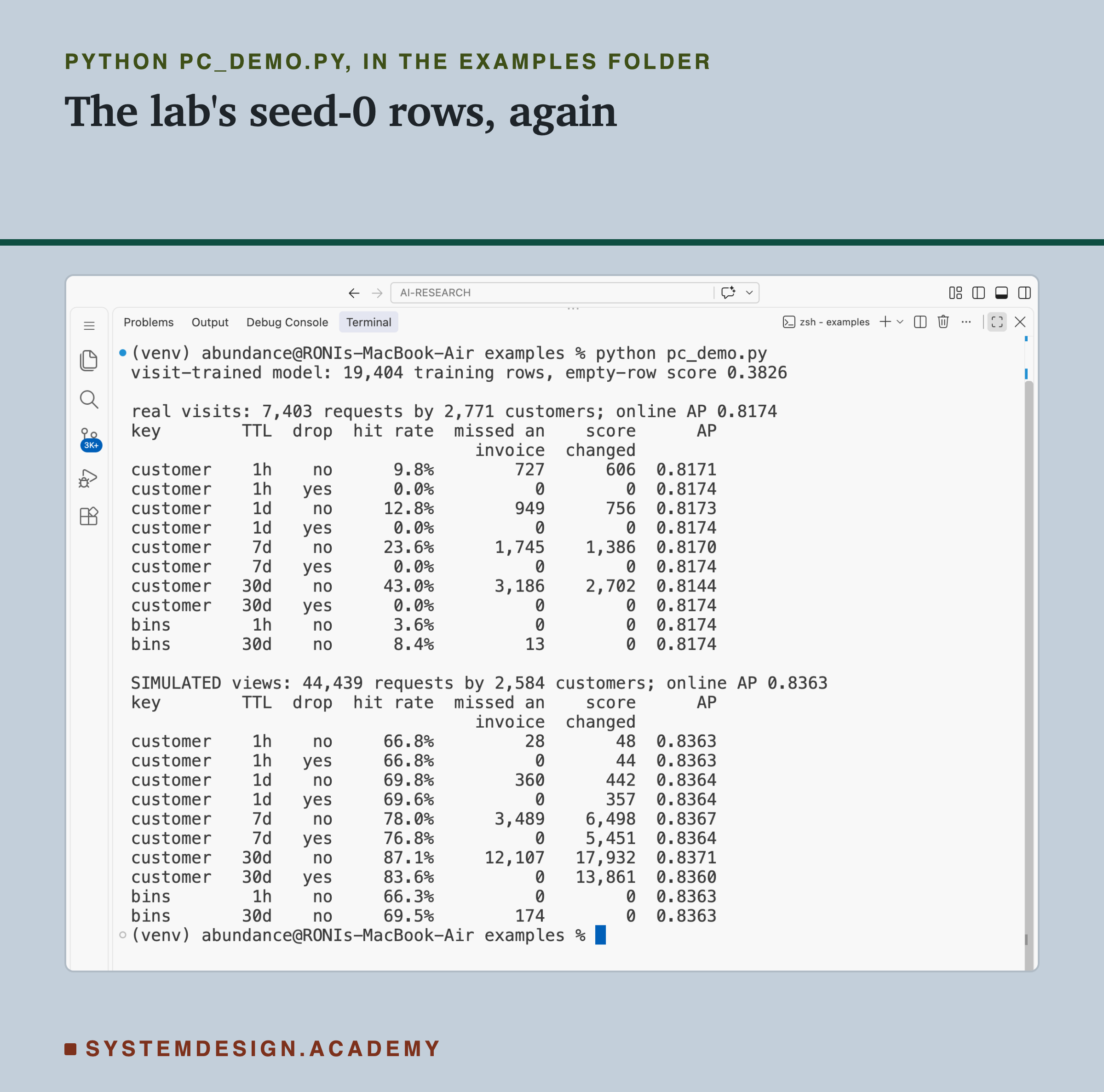
This is a real recording of the report script, pc_report.py, on the laptop where the lab ran.

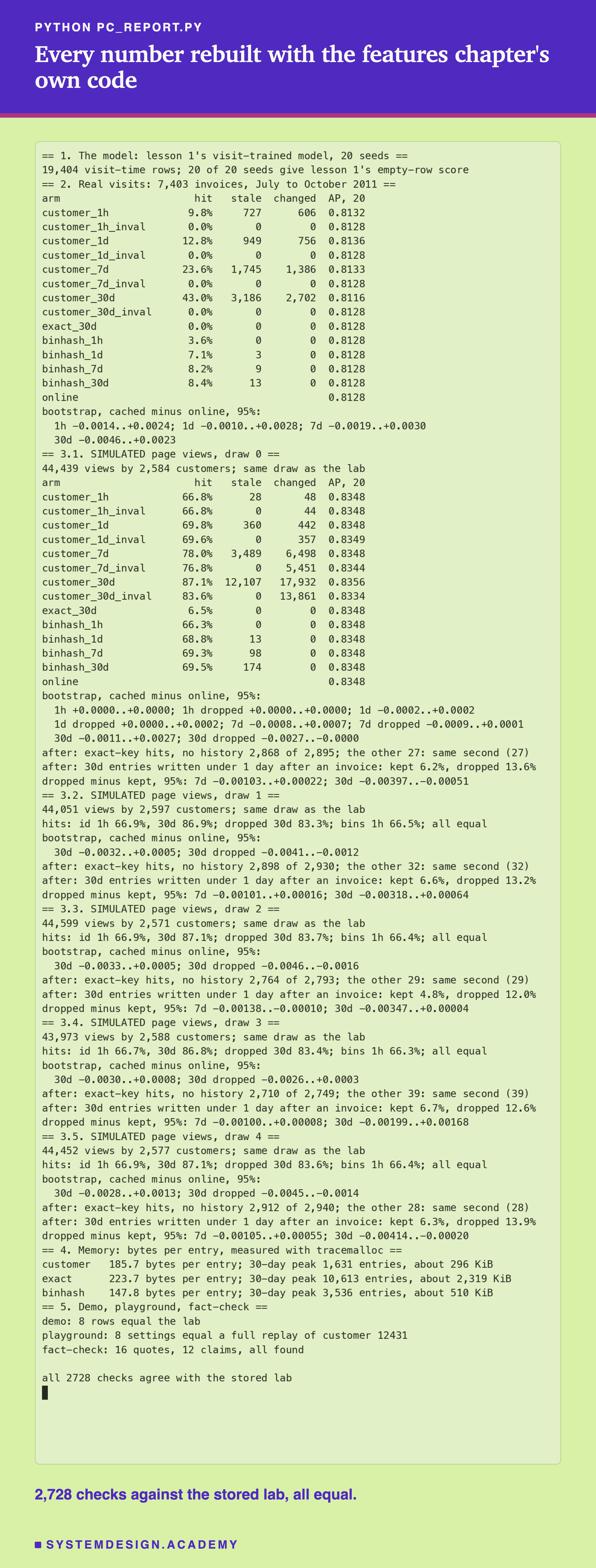
The report does not trust the lab. It never imports the lab's code, or lesson 1's. It builds every feature with the features chapter's own function, build_tables, once per customer, with that customer's request times as the moments to measure at. The lab used lesson 1's faster one-pass code instead.

It draws the simulated page views again with its own code and checks that each draw has the same fingerprint as the lab's. It replays the cache in a different way. It decides each hit from the last write of each key, without the lab's queue. And it counts the live entries from each entry's lifetime with numpy. It scores AP with scikit-learn and redoes every bootstrap with an AP function written inside the report. Then it checks the post-results part, the post-review comparison of dropping with keeping, the memory sizes, the demo, the playground and the fact-check.

Before any cache, here is the shape of the real requests. A cache keyed by customer can only hit when the same customer comes back within the TTL.

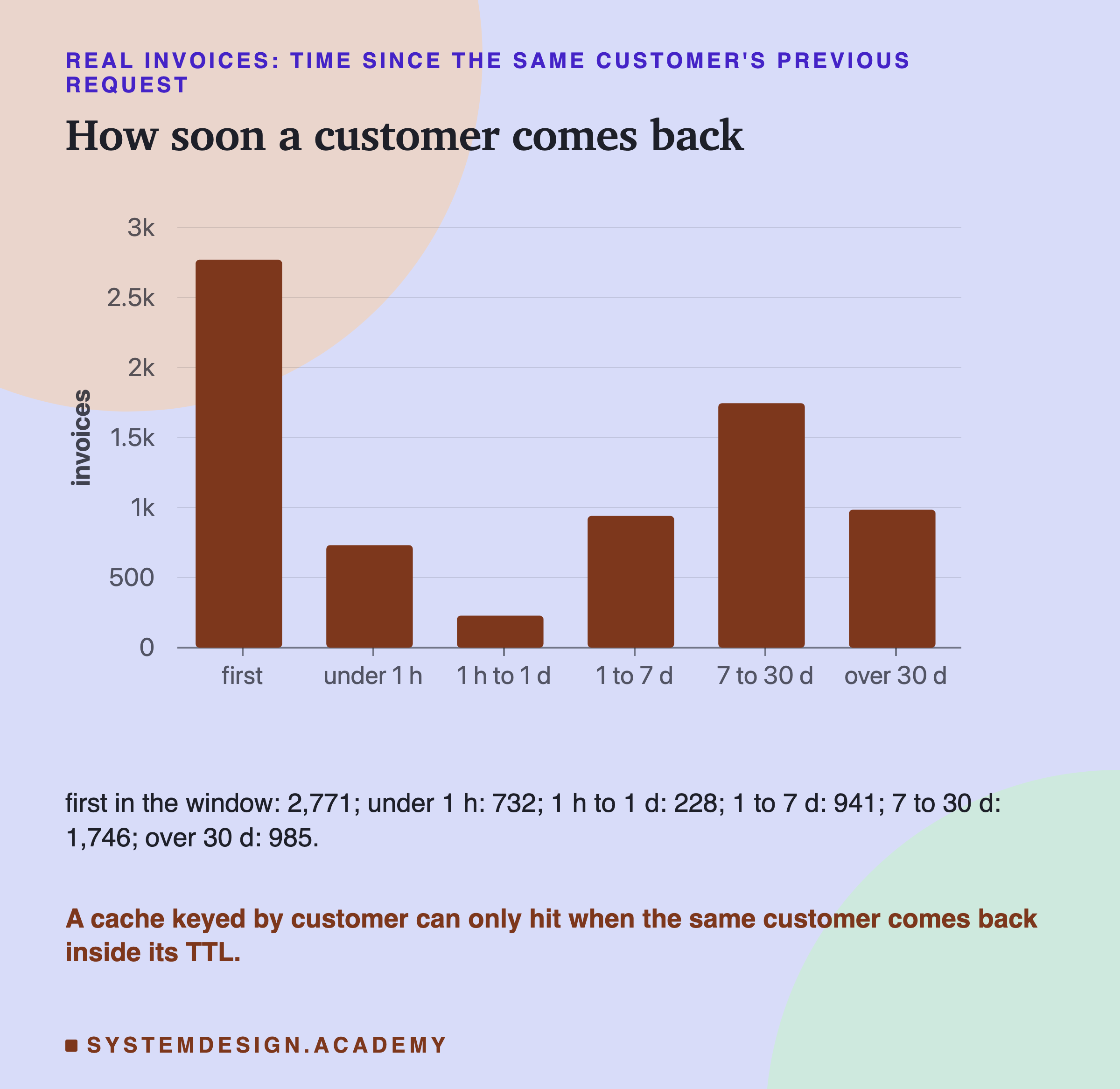
Of the 7,403 invoices, 2,771 were a customer's first in the four months, so nothing could be in the cache for them. Then 732 came less than an hour after the same customer's previous invoice. These are customers who place two or three orders in a row, for example after forgetting an item. Another 228 came within a day, 941 within a week and 1,746 within a month.

So even before running anything, you can see that a 1-hour cache on real invoices can hit at most about one request in ten. A 30-day cache can hit more, but its stored scores will often be weeks old.

Here is the first result: the hit rate of each key on the real invoices, with a 30-day TTL.

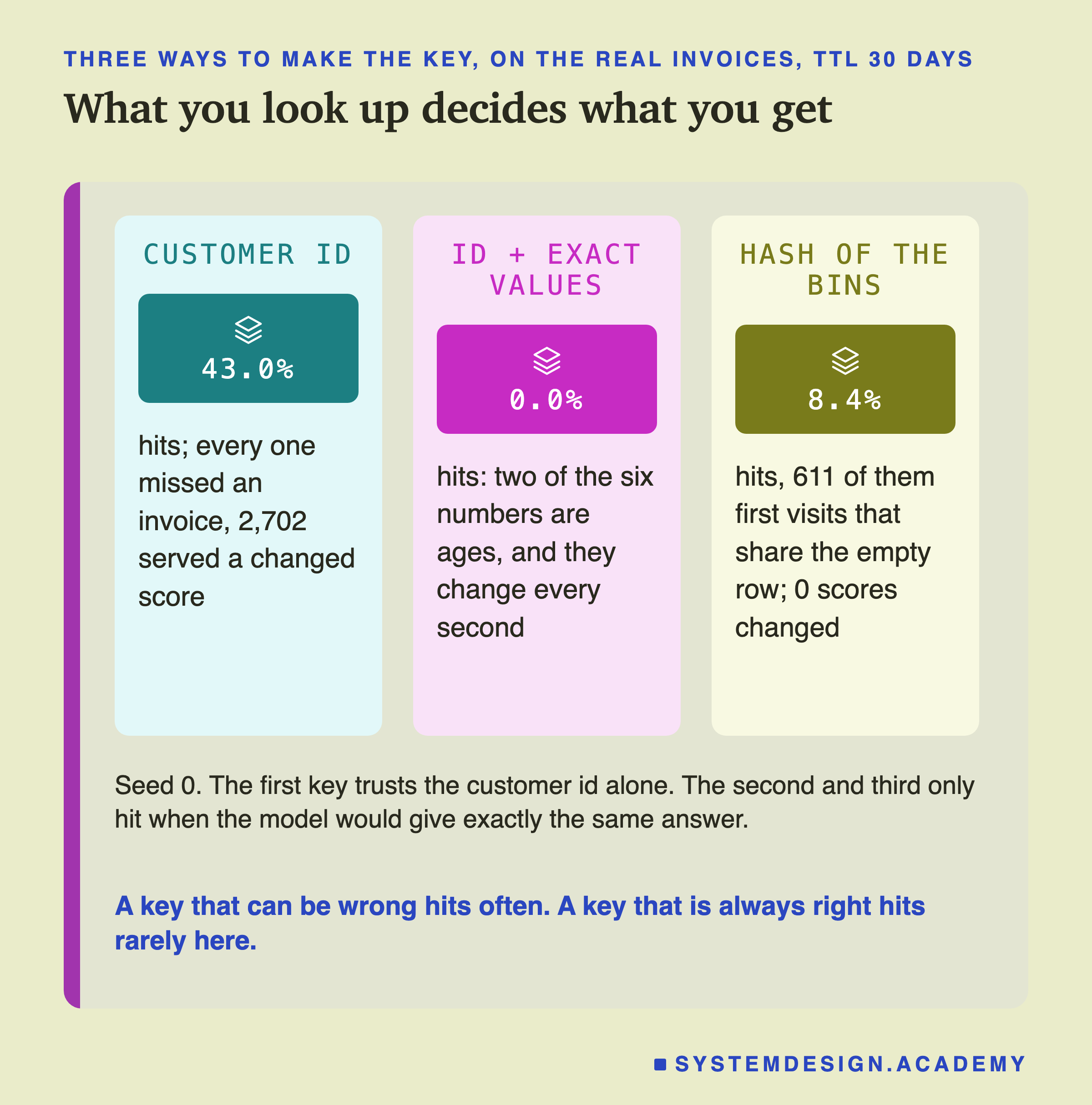
The customer key hit 43.0% of the real invoices at 30 days. Every one of those 3,186 hits had missed an invoice, as the design said it must. And 2,702 of them served a score different from the one the model would give at that moment.

The exact key hit 0 times. I expected that. Two of the six numbers, recency (days since the last invoice) and tenure (days since the first), are ages. They grow every second. So the same customer one minute later already has a different key.

The bins key hit 8.4%, and 611 of its 625 hits were a customer's first visit. A first visit has no history, so all six numbers are missing, and every such row gets the same key and the same score. Not one bins-key hit served a changed score.

Here are all four TTLs for the customer key on real invoices.

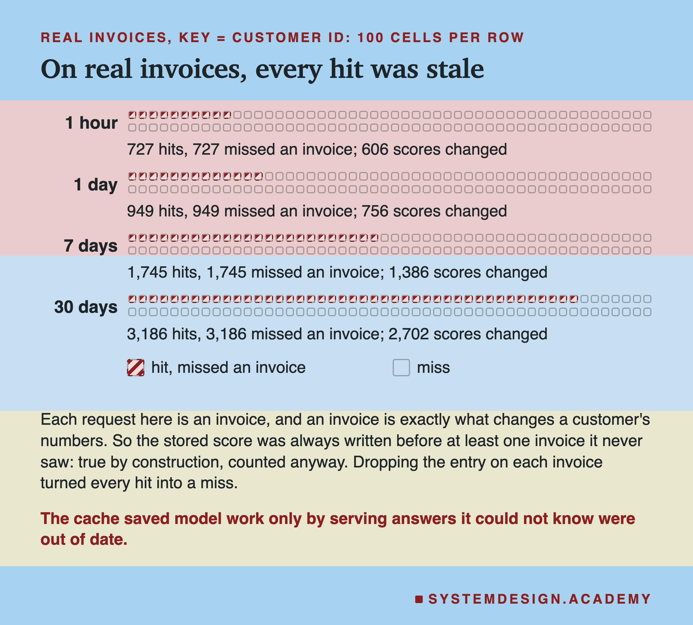
The hit rate grew with the TTL: 9.8% at 1 hour, 12.8% at 1 day, 23.6% at 7 days and 43.0% at 30 days. Every hit missed an invoice, the by-construction fact from slide 7, and the counts match it exactly.

What is not by construction is how many served scores actually changed. At 1 hour, 606 of the 727 hits served a score different from online. The model is a set of trees, and one new invoice changes the purchase count and the recency, which often crosses a split point inside a tree.

With invalidation on, the real stream had no hits at all, at any TTL. Every entry was dropped by the very invoice that wrote it. On real invoices, a cache that is never stale is a cache that never hits.

Stale is not the same as costly. The question that matters is whether the served scores rank buyers worse than online scores do.

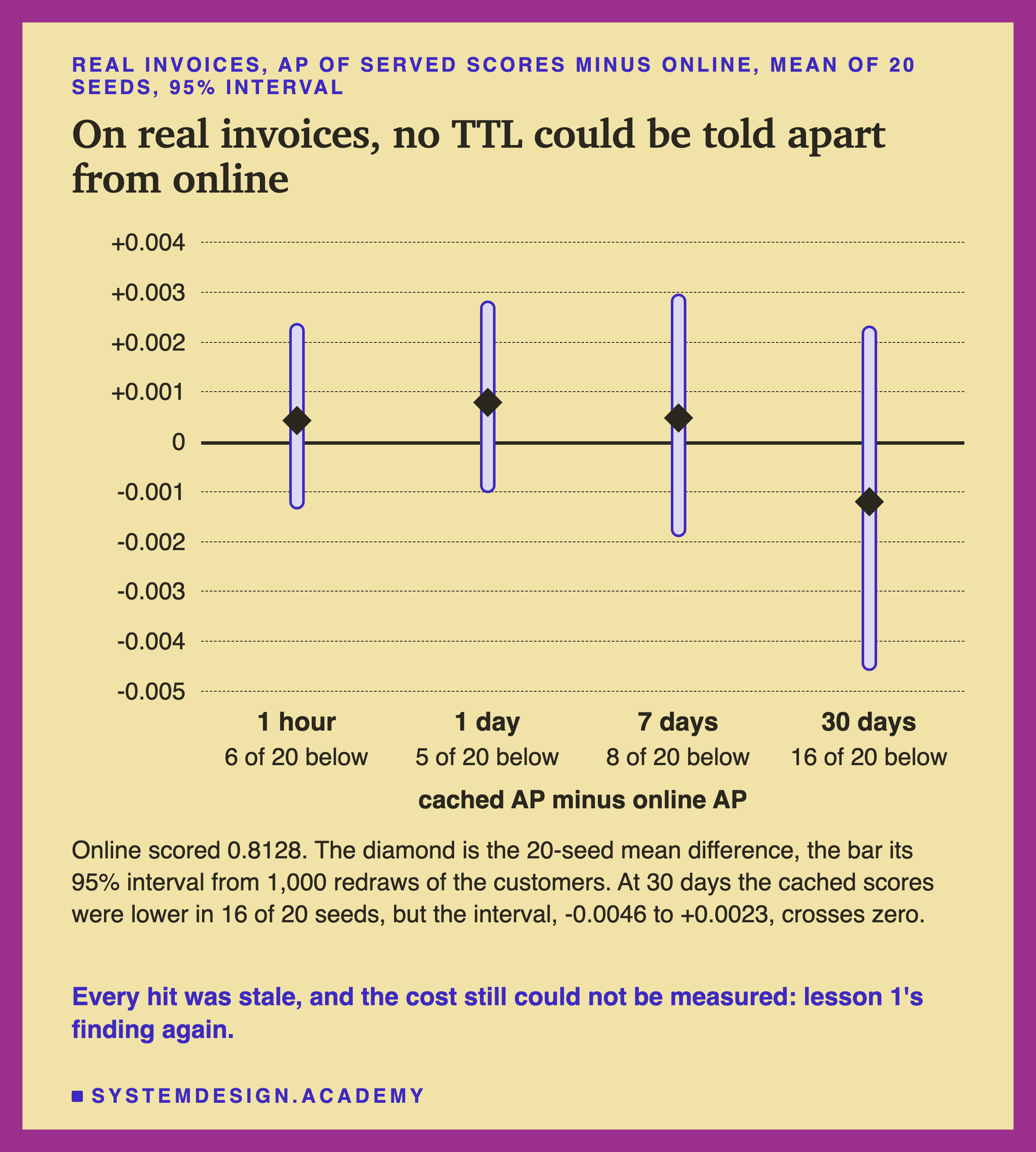
Online scoring gave AP 0.8128, the mean of 20 seeds. For every TTL, the 95% interval of the difference crosses zero. At 30 days it went from -0.0046 to +0.0023.

The seeds lean one way at 30 days: the cached scores were lower in 16 of 20 seeds. A lean is not a finding. The bootstrap says customer luck alone could make a gap this size. So my words are: on real invoices, no TTL up to 30 days could be told apart from online.

What does a difference of 0.002 AP mean? AP goes from 0 to 1, and online scored about 0.81. A change of a few thousandths means the ranking of buyers above non-buyers moved a little, for a few customers. Here every such gap was smaller than the change you get by redrawing which customers happened to visit, so none of them is a finding.

This is lesson 1's result in a new form. There, a monthly batch score up to 30.7 days old could not be told apart from a fresh one, and the same visit-trained model gave -0.0037 to +0.0031. A stale cached score is an old score, and on this slow 30-day question, old scores cost little.

Numbers over thousands of requests hide what happens to one customer. I fixed a rule before the run: take the smallest customer id with at least 4 invoices in October 2011, and show what a 7-day cache served. After the run I added a 30-day view of the same visits, and I label it so.

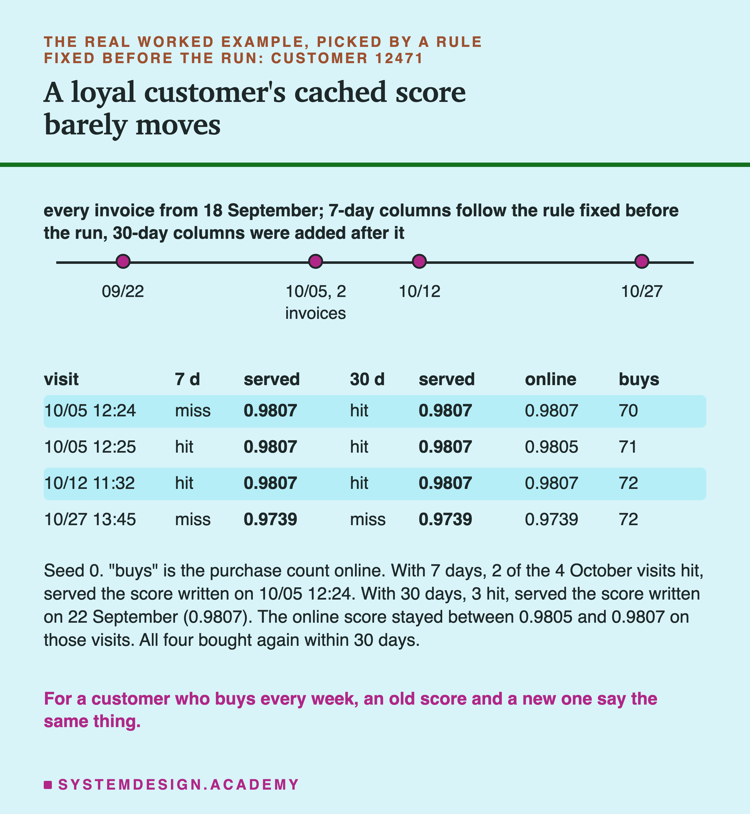
Customer 12471 is a busy buyer. With the rule's 7-day cache, the first October visit, at 12:24 on 5 October, was a miss and wrote an entry. The next visit, one minute later, and the visit of 12 October were hits. Both were stale: an invoice had come in since the entry was written, and the purchase count online went from 70 to 72.

With a 30-day cache, which I looked at only after the run, the entry from 22 September was served on three October visits.

But look at the scores. Every served score was 0.9807. The online scores on the same visits were 0.9807, 0.9805 and 0.9807. The customer did buy again after every visit. For a loyal customer, the model is sure either way, and one more order changes almost nothing.

This is one customer. It shows how a stale hit can be harmless. It says nothing about how often.

The exact key sounds like the safest choice: only reuse a score when the input is exactly the same. Here is why it barely works for this model.

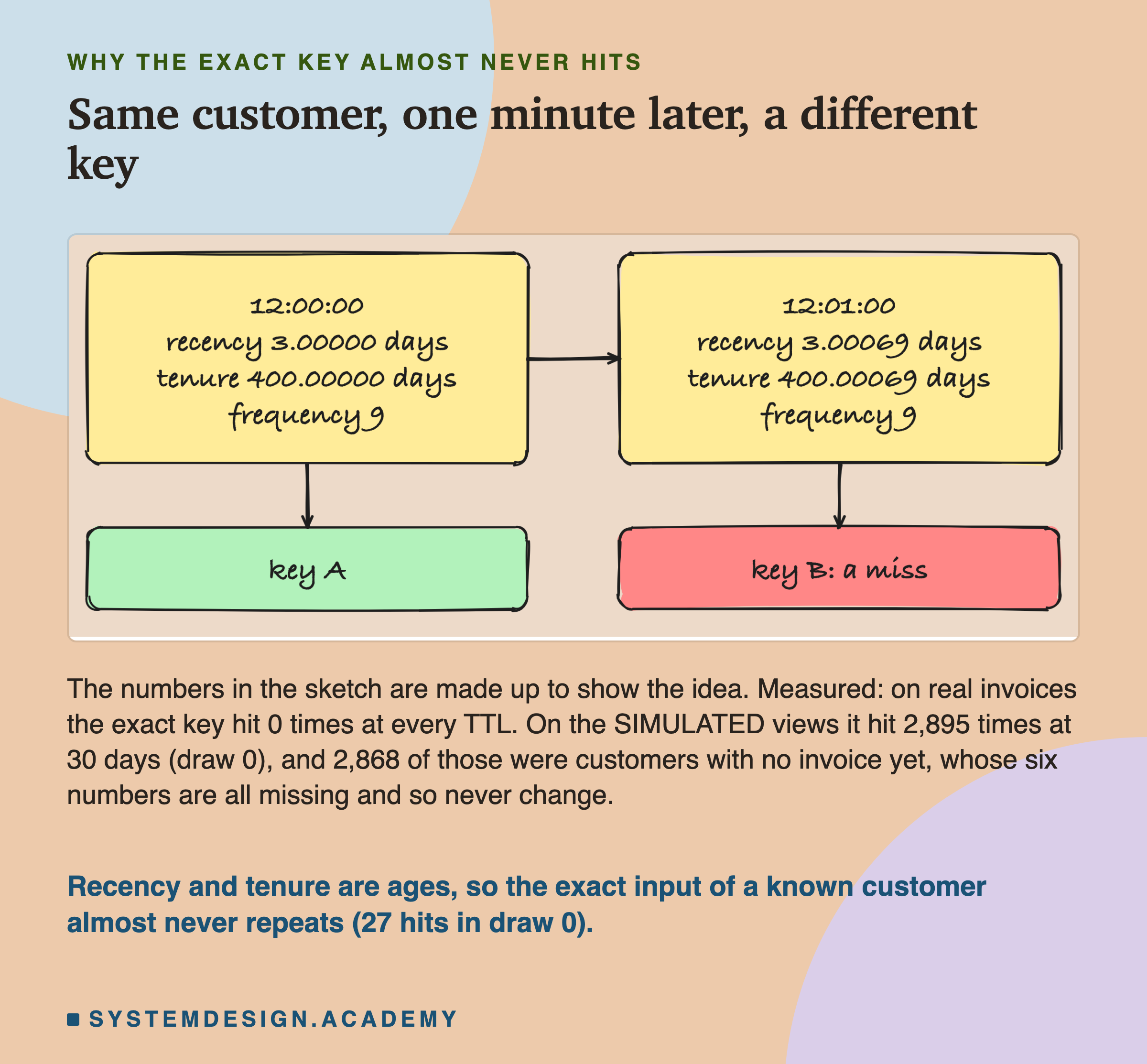
The sketch uses made-up numbers to show the idea. One minute later, the same customer has a recency and a tenure that are one minute larger. The key is different, so it is a miss.

The measured numbers agree. On real invoices, the exact key hit 0 times at every TTL. On the simulated page views it did hit, 5.3% to 6.5% of requests (the mean of five draws, from 1 hour to 30 days). I did not expect that, so after the results I looked at which requests they were. In draw 0, 2,868 of the 2,895 hits at 30 days came from customers with no invoice yet, whose six numbers are all missing. The report checked the other 27. Each was a second simulated view in the same second as the one before it, a side effect of how I drew the times.

So for a model whose inputs include an age, an exact-input cache is close to useless, except for brand-new customers.

Real invoices made every customer-keyed hit stale by design. To see how a cache behaves when requests do not change the inputs, I needed page views. Here is exactly how I made them.

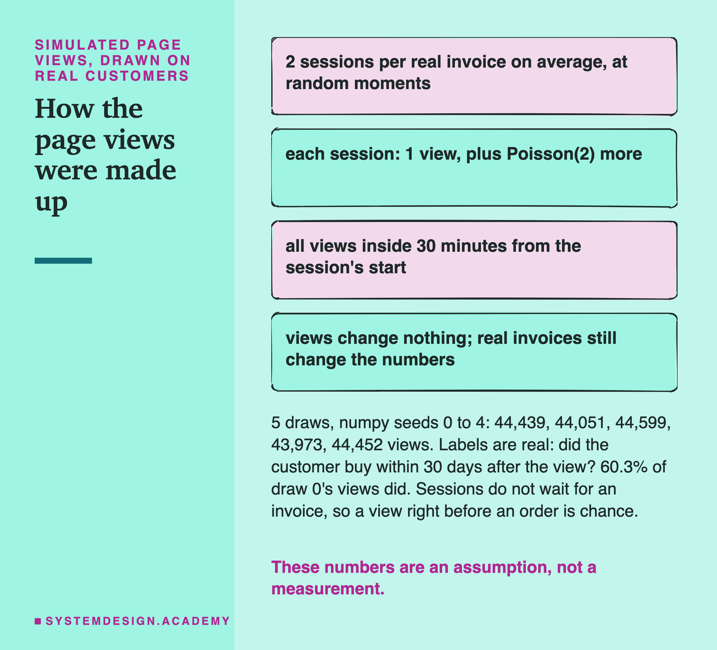
Each customer who had at least one real invoice in the four months gets browsing sessions. The number of sessions is random, around 2 for each of their real invoices. A session starts at a random second. It has one page view plus a random number more, 2 more on average, all within 30 minutes.

Poisson(2) means a random whole number that is 2 on average: often 1, 2 or 3, sometimes 0 or 5. Each draw gave about 44,000 views.

The labels are real. For each view, I ask the same question as lesson 1: did this customer buy within 30 days after it? In draw 0, 60.3% of views came from customers who did.

The real invoices still happen in the background. They change the customer's numbers, and with invalidation on, they drop the customer's cache entry.

Here are all the hit rates in one picture: real invoices on the left, simulated views on the right.

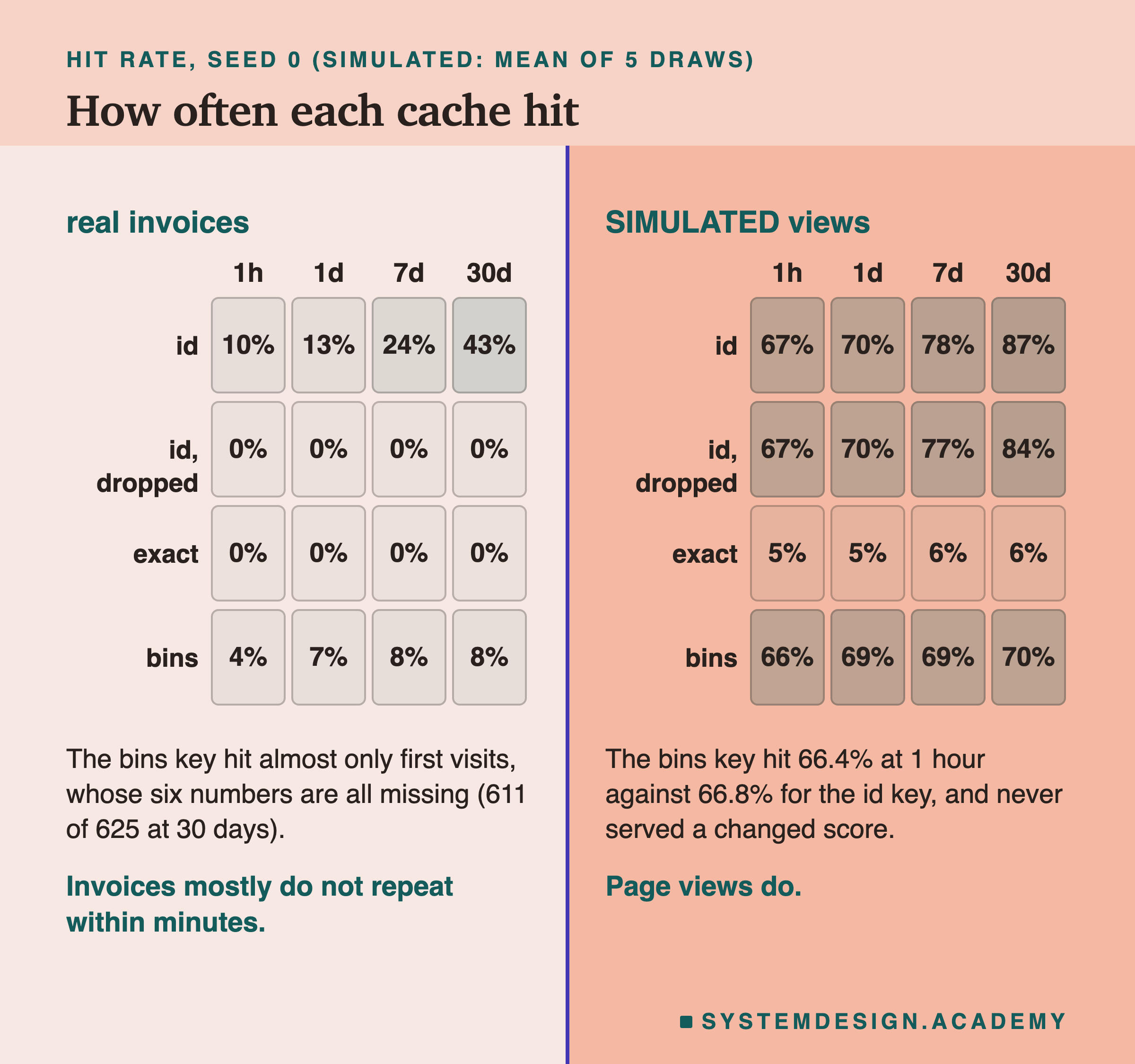
The two halves look like two different worlds. On page views, the customer key hit 66.8% of requests at 1 hour, and 87.0% at 30 days, the mean of five draws. Most of the hits at 1 hour come from views later in the same session.

With invalidation, the hit rate barely fell: 66.8% at 1 hour, 83.5% at 30 days. Invoices are rare next to page views, so dropping an entry on each invoice costs few hits.

The surprise is the bins key. It hit 66.4% at 1 hour, almost as much as the customer key, and it never served a changed score. Slide 21 explains why.

On page views, a hit is no longer stale by design. So now staleness is a real measurement.

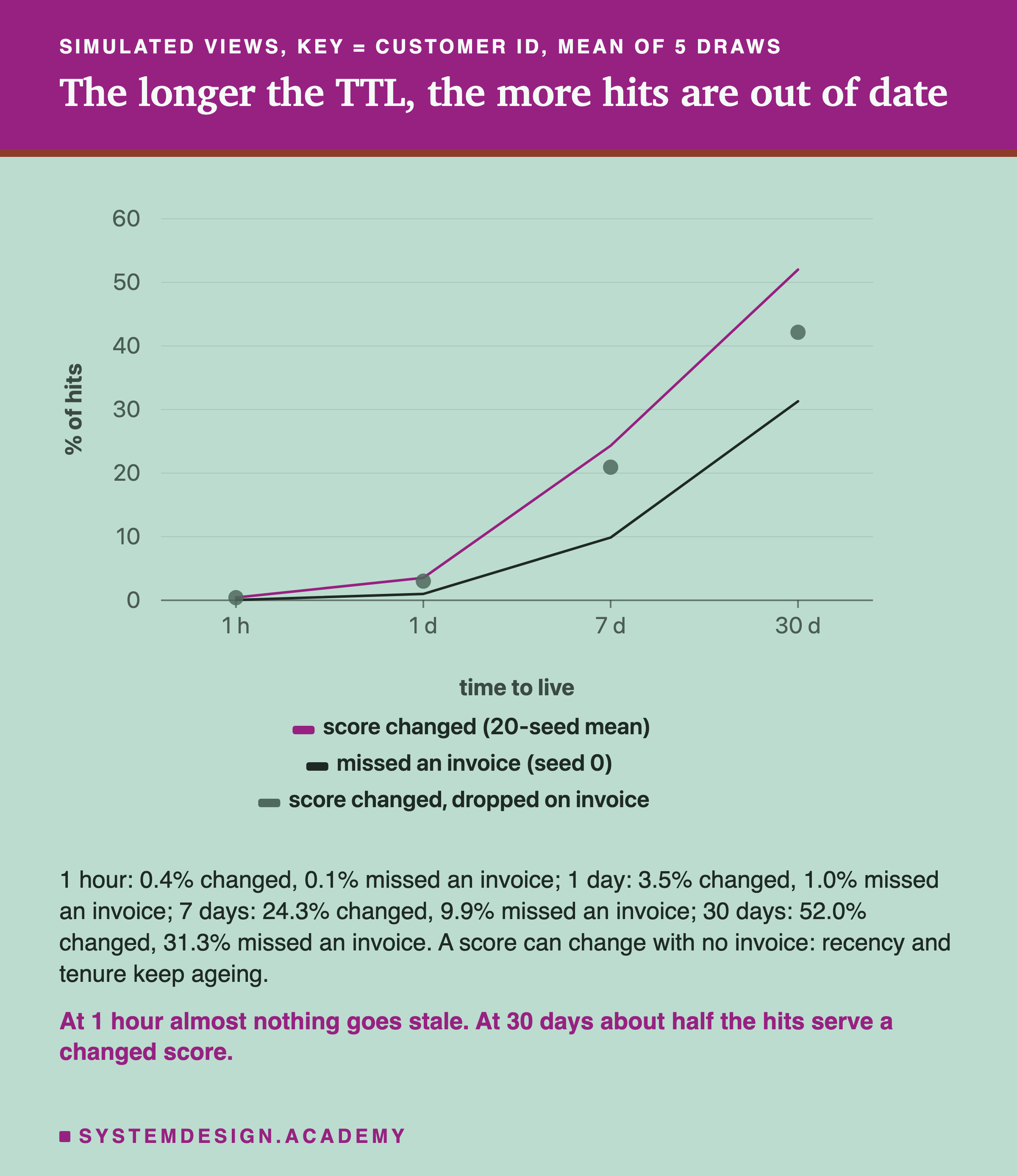
At 1 hour, only 0.4% of hits served a score different from online. At 1 day it was 3.5%, at 7 days 24.3%, and at 30 days 52.0%.

Notice that more scores changed than missed an invoice. At 30 days, 31.3% of hits had missed an invoice, but 52.0% served a changed score. The difference is the clock. Recency and tenure grow every second, so after enough days, a customer's numbers cross a split point in a tree even with no new invoice.

Invalidation removes the invoice part, but not the clock part. So with entries dropped on each invoice, 42.2% of hits at 30 days still served a changed score.

Now the cost. I expected long TTLs to cost a little AP and invalidation to win some of it back. The second half was wrong.

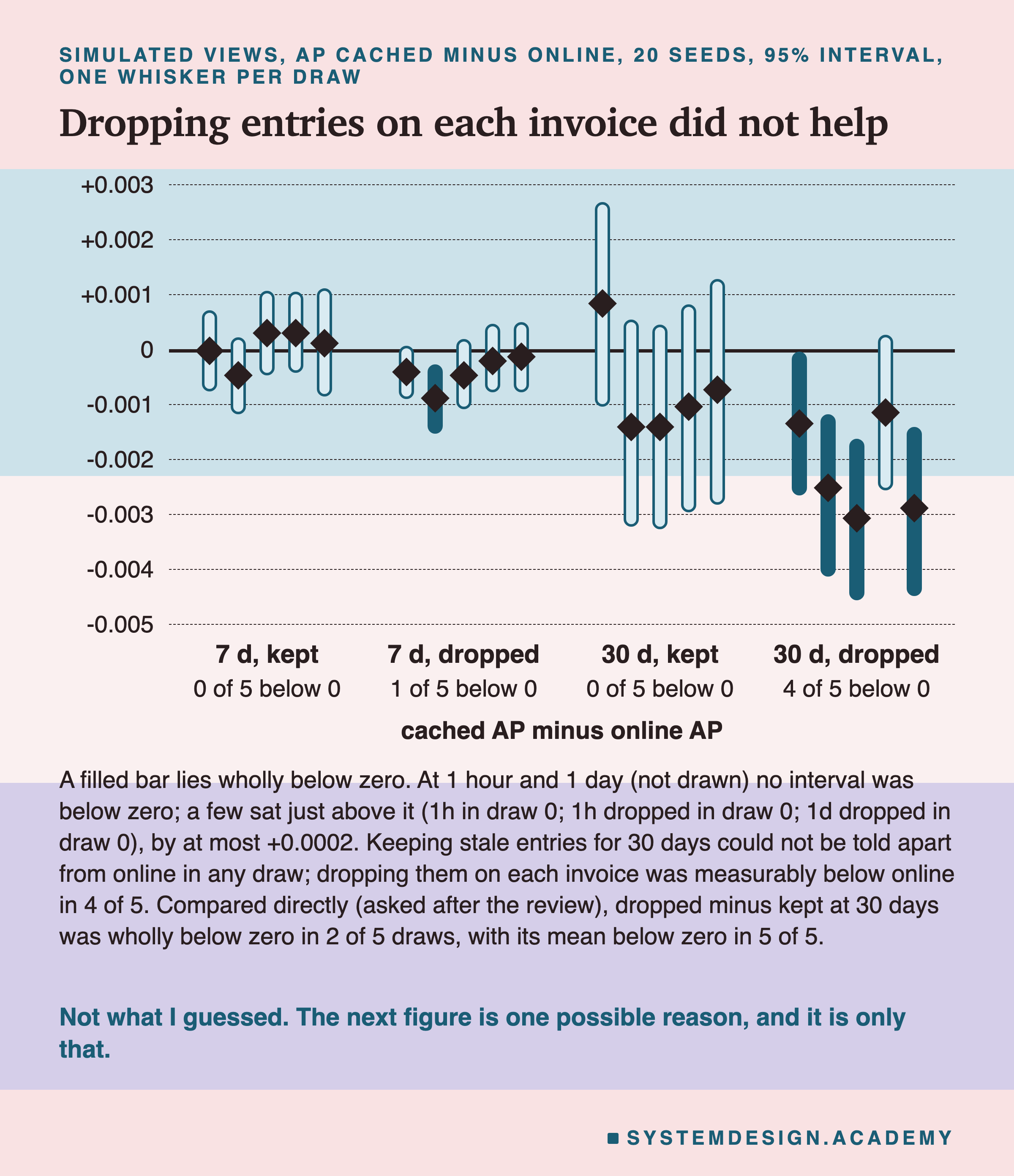
At 1 hour and 1 day, no interval in any draw was below zero. Three sat just above zero, all in draw 0: the 1-hour cache, kept and dropped, and the 1-day cache with dropping. Those gaps were tiny, at most 0.0002 AP, and the other four draws crossed zero. So I read them as the luck of one draw, not as caching helping. At 7 days, kept entries crossed zero in all five draws, and dropped entries were below online in one draw, from -0.0015 to -0.0003.

At 30 days, keeping stale entries could not be told apart from online in any of the five draws. Dropping entries on each invoice was below online in 4 of 5 draws. The lowest was draw 2, from -0.0046 to -0.0016, and in draw 3 the interval just crossed zero, from -0.0026 to +0.0003.

Being below online and being below keeping are two different questions, and my first draft mixed them up. An independent review pointed this out, so I added a labelled post-review part to the lab: the same bootstrap, but with dropping measured directly against keeping. At 30 days, dropped minus kept was wholly below zero in 2 of 5 draws (draw 0: -0.0040 to -0.0005; draw 4: -0.0041 to -0.0002). Its mean was below zero in all 5. At 7 days it was wholly below zero in 1 of 5 draws.

So my words are: dropping was below online in 4 of 5 draws, keeping in none; compared directly, dropping was below keeping in 2 of 5 draws, with the mean below in 5 of 5. These are a few thousandths of AP. Dropping entries on each invoice did not help on this task, and it may have hurt a little.

This slide answers a question I asked after seeing the results. I wrote its design into the lab's docstring before that part ran, and the lab labels it as post-results work.

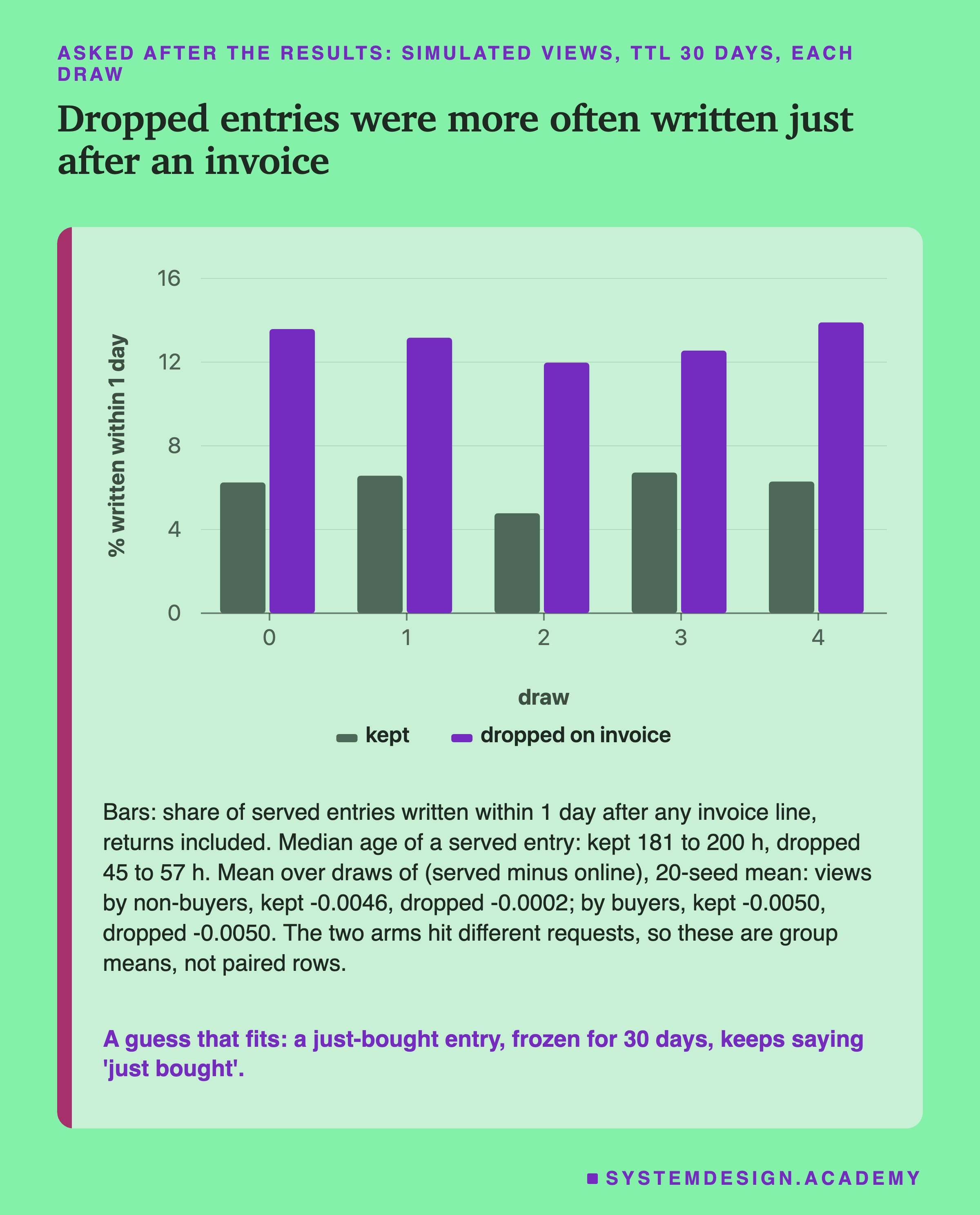
My guess, written before this part ran: when an invoice drops an entry, the next page view writes a new one, often soon after that invoice. So the entries that live under invalidation more often hold a recency close to zero: "this customer just bought". Then that entry is frozen for up to 30 days, still saying "just bought", while the online score sees the days pass.

The numbers fit the guess. Here "an invoice" means any invoice line, returns included. With entries kept, about 6% of served entries were written within a day of one. With entries dropped, about 13%.

Dropped entries were also much younger when served: a median of 45 to 57 hours, against 181 to 200 hours for kept entries. And look at customers who did not buy again. Under dropping, their cached score fell less below the online score, so they ranked a little higher than they should. For customers who did buy, the two were about the same. One caution: the two caches hit different requests, so these are averages over two different groups of hits, not the same rows compared twice.

That fits, but it does not prove the cause. Other explanations may fit too. What I can say is narrow: on this shop, with these simulated views, dropping entries on each invoice was not a free improvement.

The SIMULATED worked example uses a rule fixed before the run. In draw 0, take the smallest customer id with a stale hit under the customer key with a 1-day TTL.

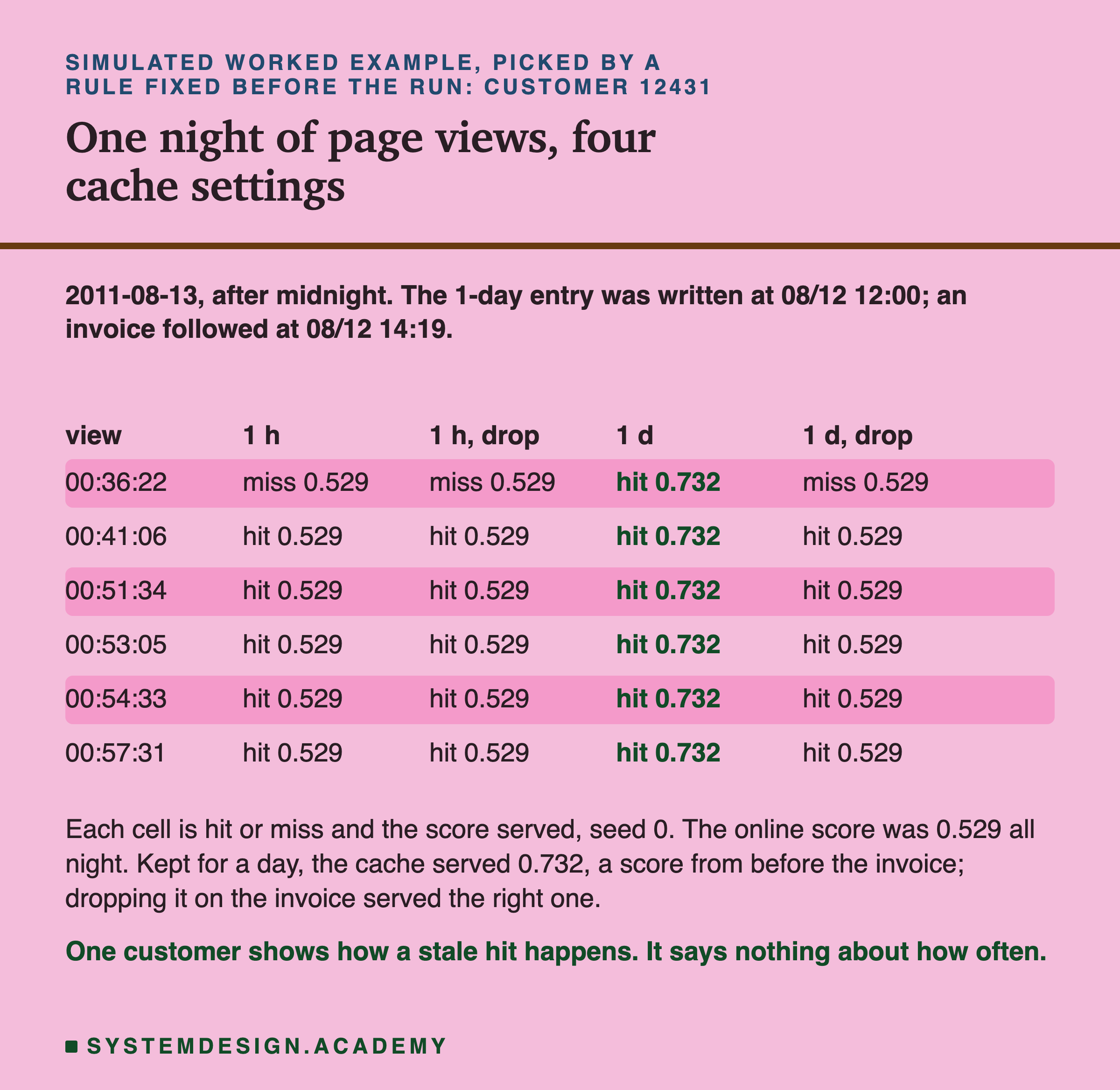
Customer 12431 browsed at noon on 12 August, which wrote a cache entry. Then they placed a real invoice at 14:19 that day. Just after midnight, they browsed again for about 20 minutes.

With a 1-day TTL and no invalidation, every view that night got the noon score, 0.732. The model, asked fresh, said 0.529, because the new invoice changed the customer's numbers. With invalidation, the invoice dropped the noon entry, the first night view was a miss, and the rest of the session got 0.529 from it.

With a 1-hour TTL, the noon entry had long expired, so the night session started fresh either way. This is the whole trade in one customer: a longer TTL gives more hits, and some of them carry news the cache never heard.

The bins key surprised me most. It hit almost as often as the customer key on page views, and it never served a wrong score.

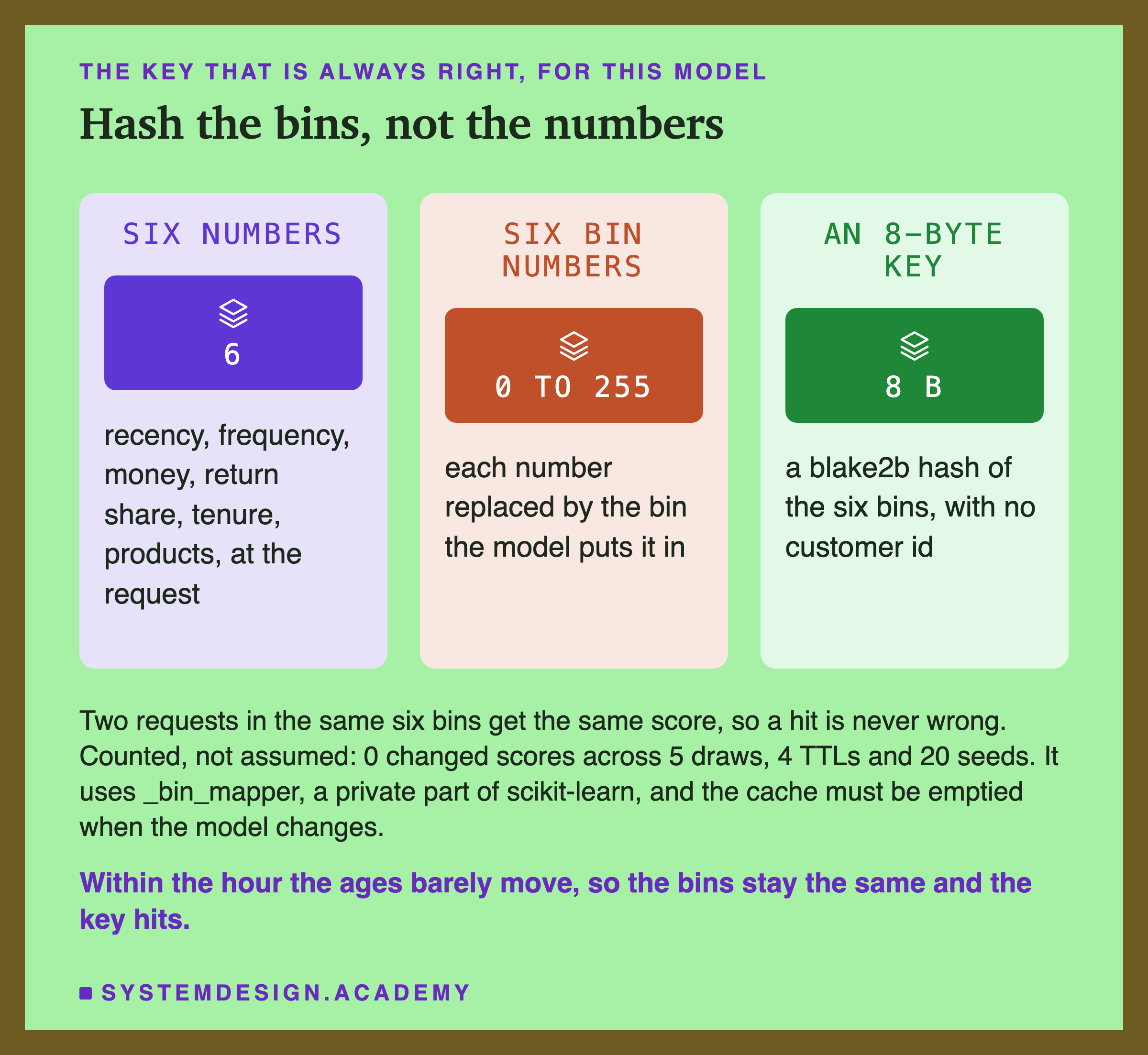
Here is the idea. The model never looks at the exact value of a number. It only asks which bin the value falls in, like "recency between 15.2 and 16.1 days". So two requests whose six numbers fall in the same six bins must get the same score.

So I made the key from the bins: six small whole numbers, turned into an 8-byte hash. Within a 30-minute session, recency and tenure grow by minutes, which almost never moves them into another bin. So the key repeats, and the cache hits.

I did not trust this argument. The lab compared every served score with the online score, for every draw, TTL and seed. Not one differed.

Why did the bins key hit so often? I checked this after the results, and the lab labels it as post-results work. Many customers had no invoice yet when they browsed, so their six numbers were all missing, and all of them share one key. In draw 0, 2,693 of the bins key's hits at 1 hour were such rows. Every other hit at 1 hour came from the same customer, within the hour.

Three warnings. The bins come from _bin_mapper, a private part of scikit-learn that can change in a new version. The key belongs to one trained model, so the cache must be emptied whenever the model changes. And this trick only works for a model that bins its inputs, like this one.

AP summarizes the whole ranking. A shop often acts only on the top, so I also counted the top fifth.

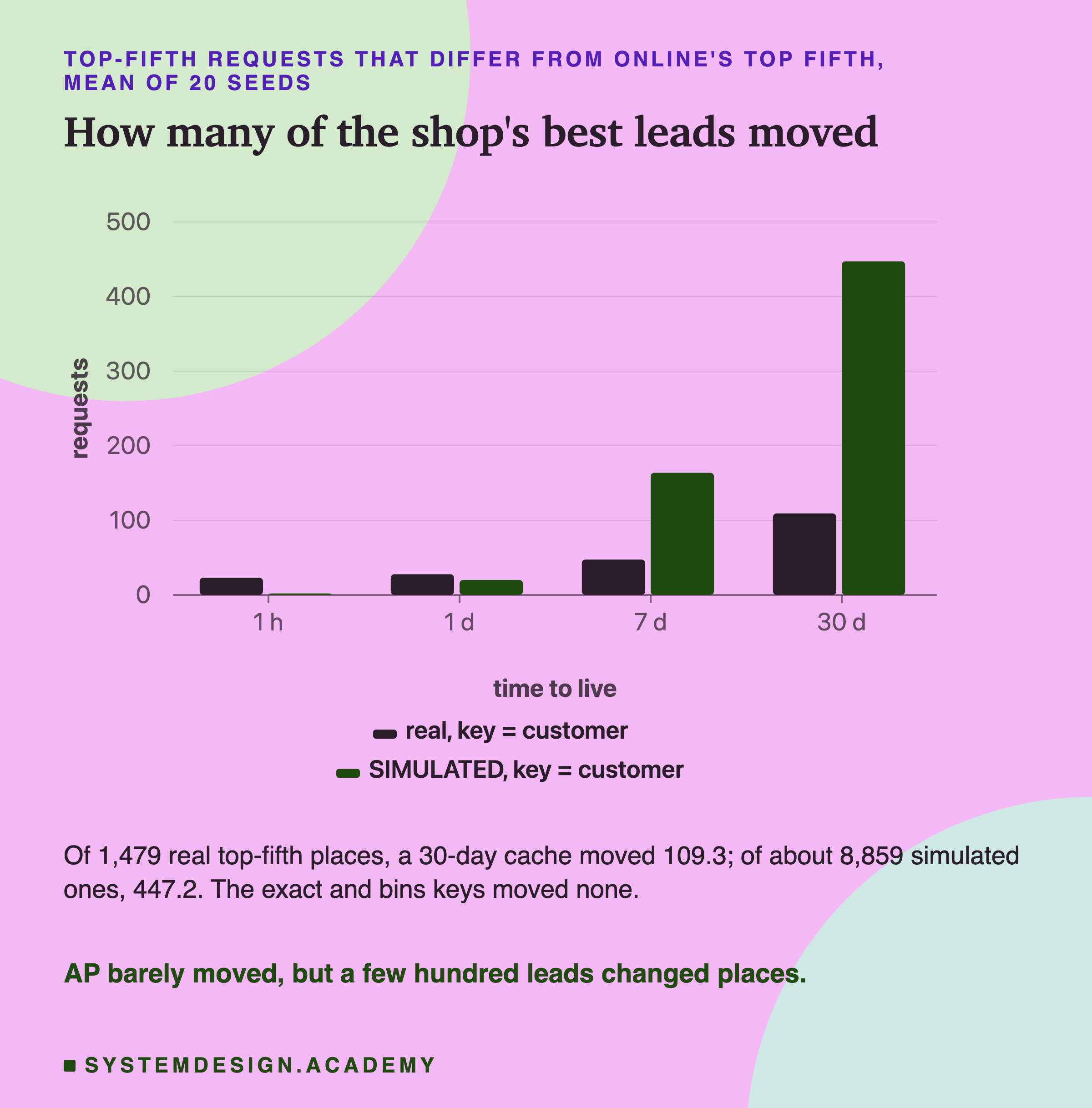
The top fifth is the 20% of requests each month with the highest scores. I counted the requests that were in the top fifth by the served scores but not by the online scores.

On real invoices, a 30-day customer cache moved 109.3 of 1,479 top-fifth places, the mean of 20 seeds. On the simulated page views it moved 447.2 of about 8,859, the mean of five draws. At 1 hour, almost nothing moved in the simulated views: 2.0 places.

So the ranking as a whole stayed about as good, but a few hundred specific customers swapped in and out of the top. If your shop sends a coupon to the top fifth, a long TTL changes who gets it, even when AP cannot see the difference. The exact and bins keys moved no one, because they never served a changed score.

A cache costs memory. I measured two things: how many entries each cache held at its busiest moment, and how many bytes one entry takes.

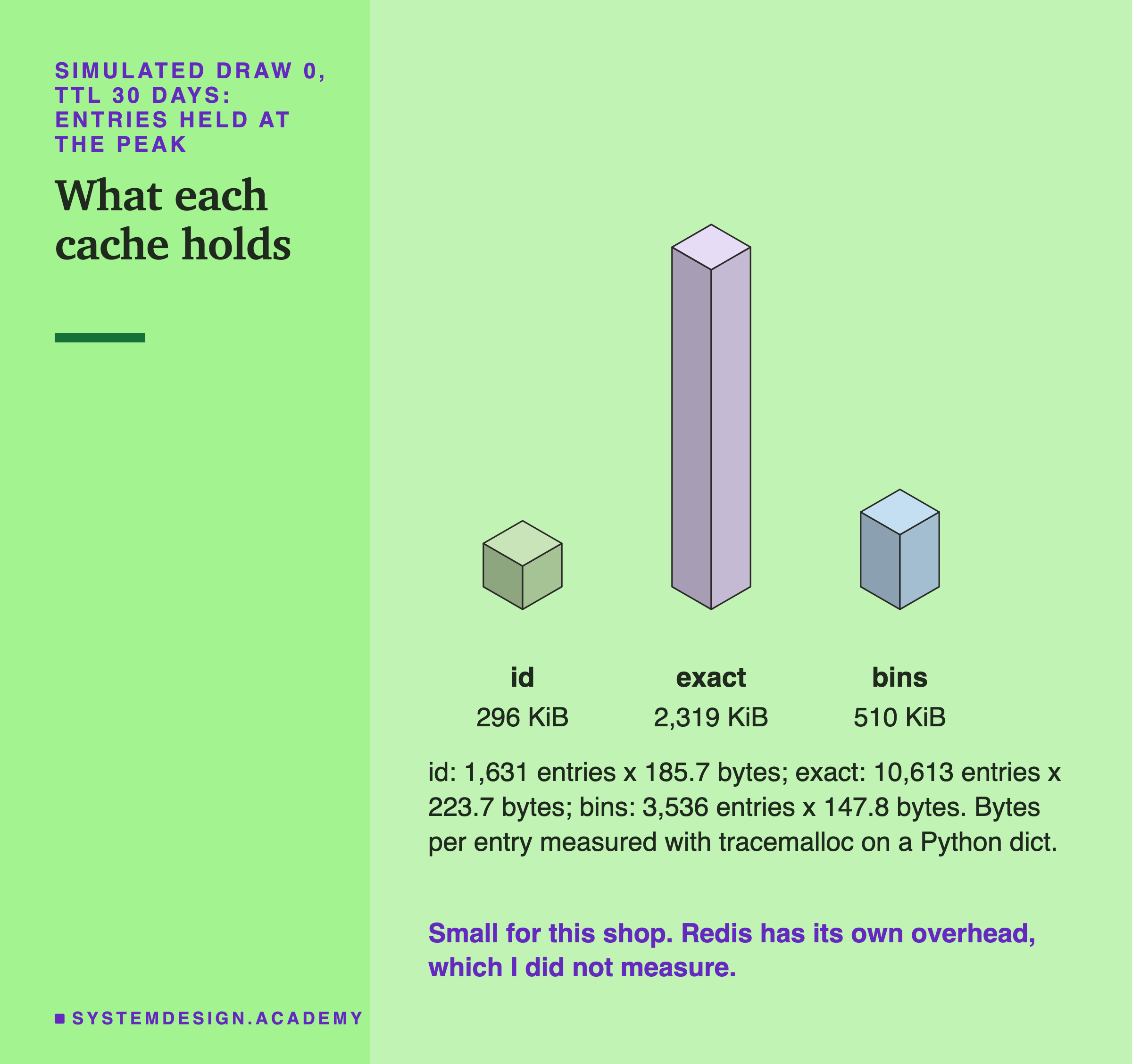
The peak is the most entries alive at any moment. At 30 days on draw 0, the customer key held at most 1,631 entries, one per active customer. The exact key held 10,613, because every miss writes a new key and the old ones live on until their timer ends. The bins key held 3,536.

For bytes per entry, I used Python's tracemalloc, a tool that counts the memory Python hands out. I built a dictionary of real keys, each mapped to a score and a write time, and divided the memory by the number of entries, five times. A customer entry took 185.7 bytes, an exact entry 223.7 and a bins entry 147.8. These are Python numbers on one laptop. A Redis server stores keys its own way, and I did not measure it.

Notice the trade between hits and memory. The exact key held more than six times as many entries as the customer key, for far fewer hits. Most of its entries were written once and never read again. The bins key sat in between: it held about twice as many entries as the customer key, and it never served a wrong score.

The bytes per entry were measured at different entry counts (5,942, 41,342 and 13,490 entries), and a Python dict grows in steps, so treat them as rough figures.

For this shop, all of it is under a few megabytes. For a site with millions of customers, the exact key would need the most memory and give the fewest hits.

This lesson and lesson 1 measured the same thing from different sides: what does an old score cost on this shop?

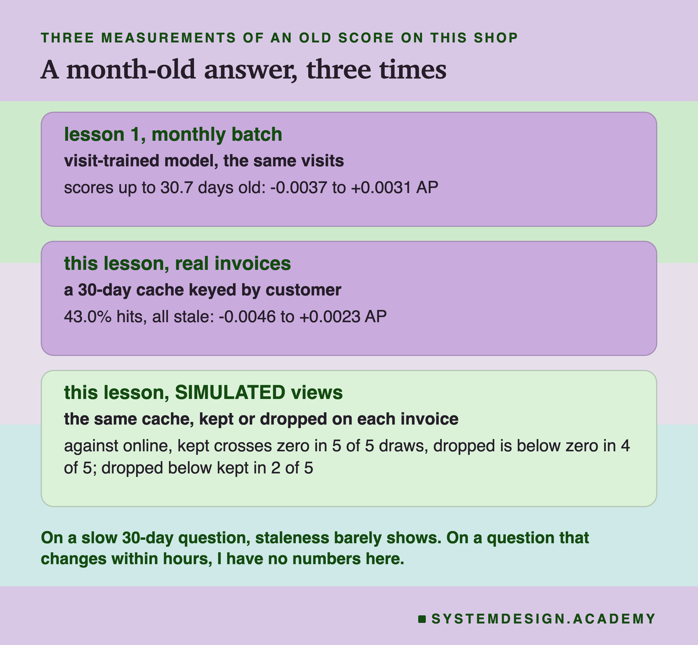
Three measurements agree on the main point. On this shop's 30-day question, a score up to a month old could not be told apart from a fresh one. That held for a monthly batch in lesson 1. It held for a 30-day cache on real invoices here. And it held for a 30-day cache that keeps its entries on simulated views here.

The only cost I could measure came from a choice that sounded safer: dropping entries on each invoice. It was below online in 4 of 5 draws, and below keeping in 2 of 5. So a cache adds a new way to go wrong that a batch does not have: the rules for when an entry lives and dies.

For a fast question, the picture would be different. The course measured one in batch vs streaming data: counting bike rentals for the next hour, where old counts nearly doubled the error. A fraud check on a card payment, or a feed that changes with every click, could lose a lot from a score that is one hour old. I have not measured those tasks here, so I give no numbers for them.

What I can say is what would change, in words. On a fast task, the share of hits that serve a changed score would climb much faster with the TTL than it did here. The right answer moves within minutes, not weeks. The clock part of staleness would matter more too: a feature like "minutes since the last click" crosses a split point quickly. So a long TTL that cost nothing measurable on this shop could cost a lot there.

And invalidation would likely matter in the other direction from what I found here, because on a fast task the newest event carries most of the signal. That last sentence is a guess, not a measurement. The way to know is the same replay this lab did, on your own requests.

I wrote five guesses into the lab's docstring before it ran. Here they are word for word, against the results.

1. "REAL, key (a): hit rate under 1% at 1 h, a few % at 1 d, about a quarter at 7 d, about half at 30 d; 100% of hits stale (by construction). AP: no TTL can be told apart from online, because lesson 1 found a score up to 30.7 days old cost nothing measurable on this question. Top-fifth differences grow with the TTL." Wrong at 1 hour and 1 day: 9.8% and 12.8%, because many customers place several invoices within minutes. Close at 7 and 30 days: 23.6% and 43.0%. Every hit was stale, as designed, and no TTL could be told apart from online. The top-fifth differences did grow with the TTL: 23.1, 27.7, 47.5 and 109.3 places.

2. "Key (b): no hit, or almost none, on either stream (the clock moves recency and tenure)." Right on real invoices. Wrong on page views: 5.3% to 6.5% (mean of five draws), almost all from customers with no history yet.

3. "Key (c): exact on every hit; on the real stream most hits are first visits sharing the empty-row key." Right on both counts: 0 changed scores, and 611 of 625 real hits at 30 days were first visits.

4. "SIMULATED, key (a): most views after the first in a session hit at 1 h; few hits stale at 1 h, many at 30 d. Invalidation removes the invoice part and costs little hit rate at 1 h. AP cannot be told apart from online at any TTL." The first parts were right: 66.8% hit at 1 hour, 0.4% of hits changed, and invalidation cost almost no hits at 1 hour. The last part was wrong both ways. Dropping entries at 30 days was below online in 4 of 5 draws, and three short-TTL caches in draw 0 sat just above zero.

5. "Memory: key (a) holds at most one entry per customer; (b) and (c) hold more keys for the same hits." Right: 1,631, 10,613 and 3,536 entries at the 30-day peak.

The full lab trains 20 models, draws five sets of page views and redraws the customers thousands of times. I wrote a smaller demo that does the heart of it with one model and one draw.

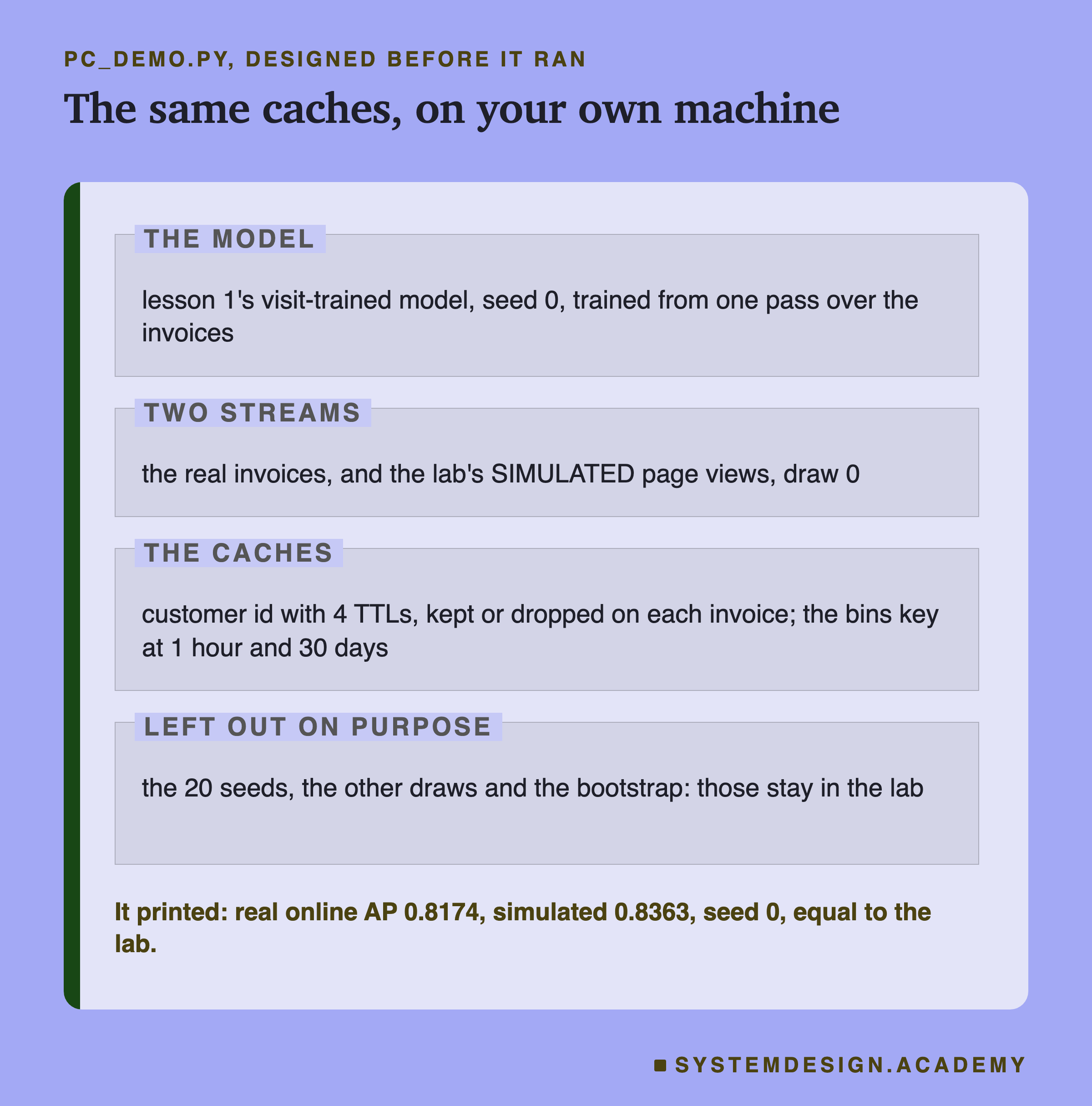
I wrote the demo's design into its docstring after the lab had run and before the demo first ran. It trains the visit-trained model with seed 0. It builds the real invoices and the lab's simulated draw 0, and works out every request's six numbers in one pass over the invoices. Then it replays each cache with a plain dictionary and a queue, and prints a table.

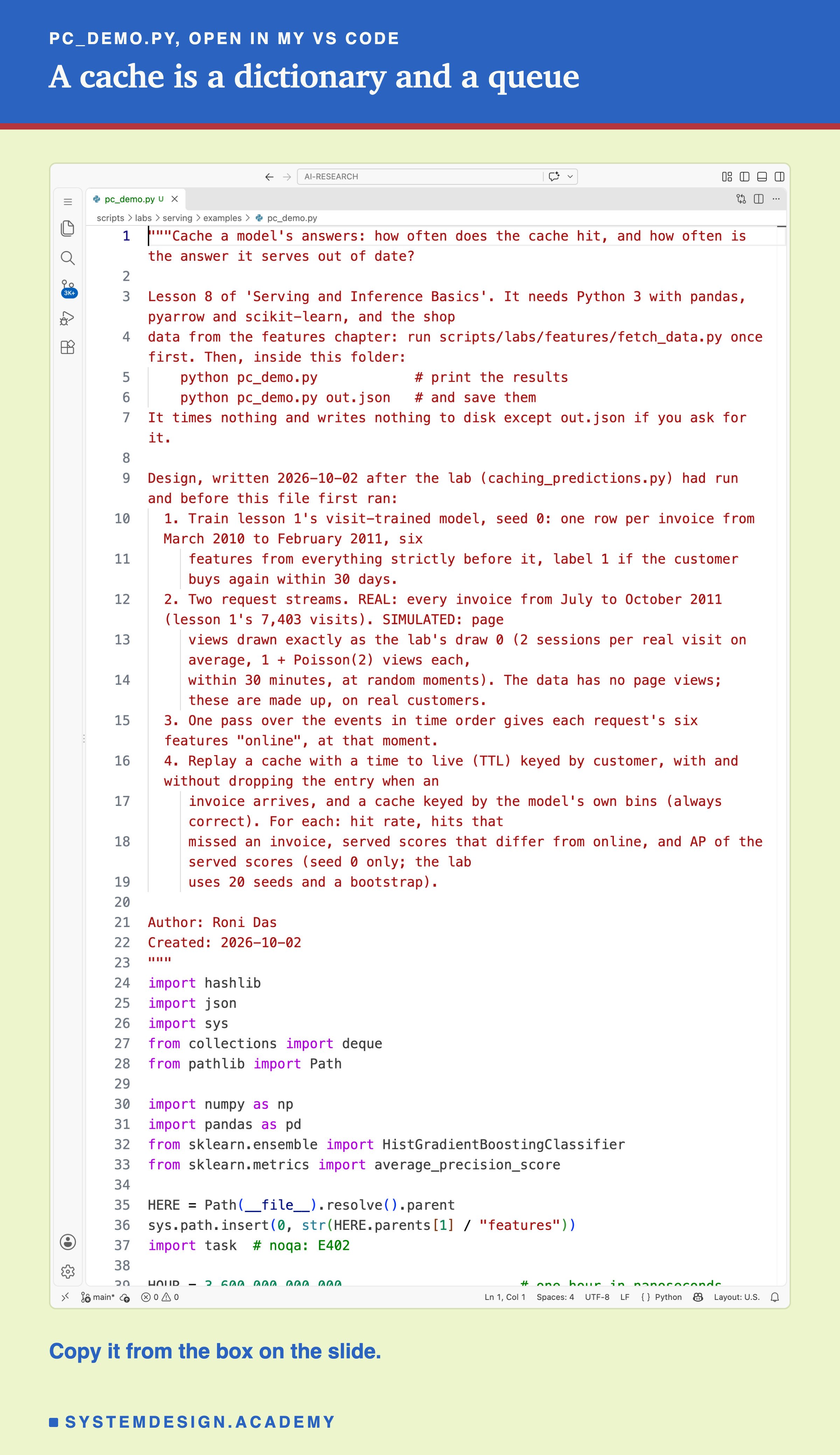
Before you run this lab. You need Python 3 with pandas, pyarrow and scikit-learn: pip install pandas pyarrow scikit-learn openpyxl. First run python fetch_data.py from the scripts/labs/features folder. It downloads the shop data once, about 46 MB, and writes one cleaned file. Then, inside the examples folder of scripts/labs/serving, run python pc_demo.py. It needs no GPU. I ran it with scikit-learn 1.9.1 and Python 3.13 on a Mac. Another version of scikit-learn may give slightly different decimals, and the bins key reads a private part of scikit-learn that a new version may change. The pattern should hold: every real hit misses an invoice, and page views hit often.

This box holds a real cache and real data from the lab. It needs nothing but Python, so it runs in your browser. It has no model inside: the scores were made by the lab's seed-0 model.

Press Run. It replays a cache keyed by customer over every SIMULATED page view of customer 12431, the customer from slide 20. All of that customer's real invoices up to October 2011 run in the background. Each line says hit or miss, and whether a hit missed an invoice. Then it prints the lab's results for the same setting: real invoices, or simulated views from draw 0.

Change TTL_HOURS to 1, 24, 168 or 720, and DROP_ON_INVOICE to True, and run it again. Watch which hits disappear.

The report script writes this box from its own replay of the data, runs it for all eight settings, and checks that the hits and stale hits it prints for this customer equal a replay of the whole stream. One customer's numbers are an example. The lab's table at the bottom is the measurement.

Try this order. First run it as it is, with a 1-day TTL. Then set the TTL to 1 hour: most hits stay, because views in one session are minutes apart, and the stale ones go. Then set it to 720 hours, 30 days, and watch how many hits now carry a score from before an invoice. Last, set DROP_ON_INVOICE to True and see which of those hits turn back into misses.

The lab is one file, scripts/labs/serving/caching_predictions.py. It imports lesson 1's code and never changes it.

Models rebuilds lesson 1's visit-trained model with 20 seeds, using lesson 1's own build_requests and snapshots. It stops unless every seed's empty-row score and online AP equal what lesson 1 stored.

simulate_views draws the SIMULATED page views with the parameters on slide 15. label_at gives each request its real 30-day label.

run_cache is the cache. It walks the requests in time order. Before each request, it applies the invoices that came before it, if invalidation is on, and removes entries whose TTL has run out. Then it looks up the key. On a hit it records which earlier request wrote the entry. On a miss it writes a new entry. It also tracks the most entries alive at once.

evaluate runs every key and TTL on one stream. For each hit it checks whether an invoice came between the write and the hit, whether the six numbers differ, and whether the served score differs from online, for every seed. Then it computes AP per month, the top fifth, and seedmean_boot, the customer bootstrap of the 20-seed mean.

bytes_per_entry measures memory with . holds the post-results questions of slides 14 and 19, and downloads each source and searches for every quote.

Here is the order of questions I would ask before caching a model's scores.

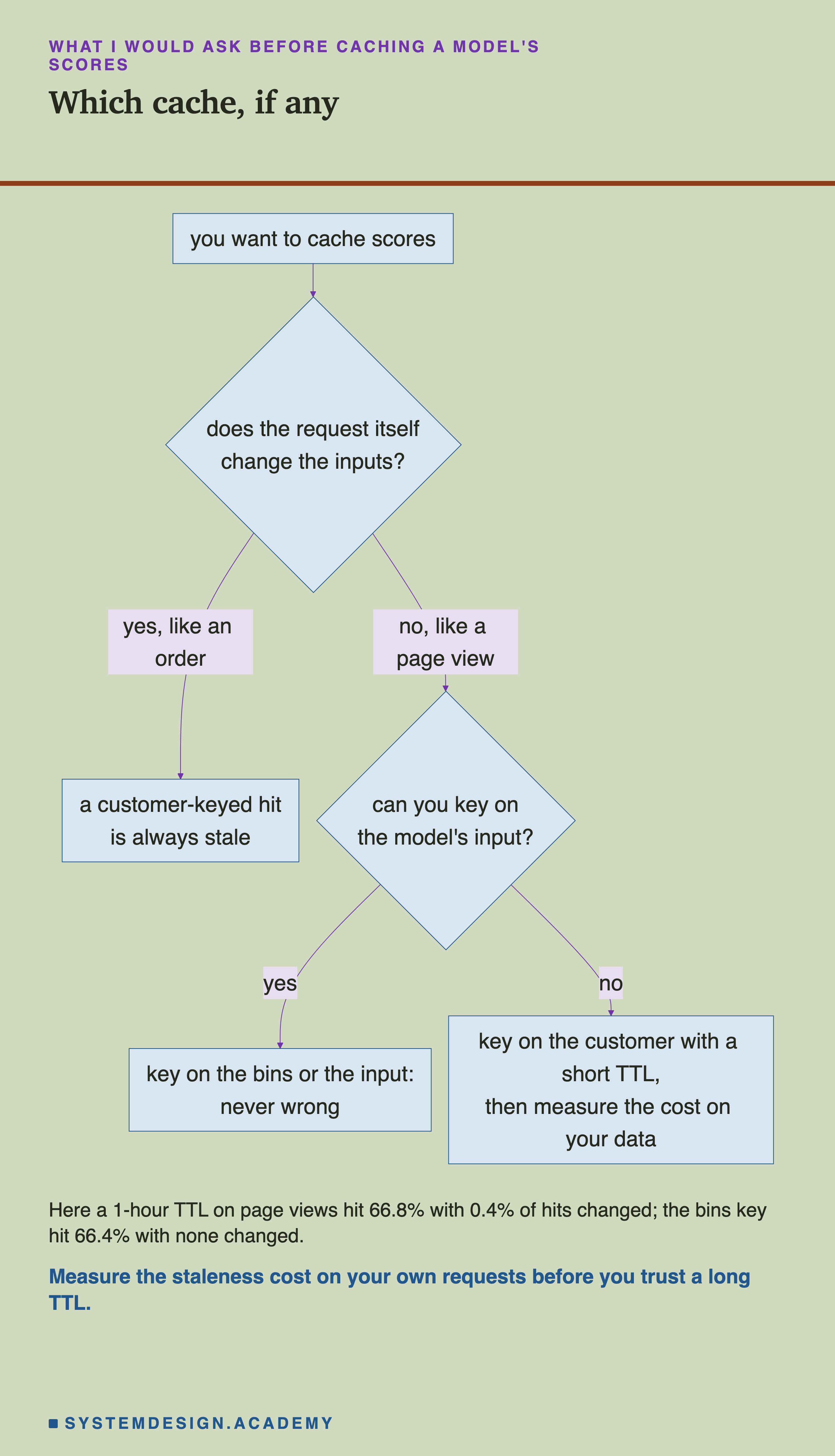
The chart asks about the request first, because on this shop that one question split the results in two: real invoices made every customer-keyed hit stale, and page views did not. Here are the same steps in words.

1. Ask whether the request itself changes the inputs. If a request is an order, a payment or a message, the customer's numbers change with it. Then a cache keyed by customer serves a stale score on every hit, by design. On real invoices here, that was 100% of hits.

2. Try to key on what the model actually sees. For a model that bins its inputs, the bins make a key that is never wrong. For other models, the exact input is a safe key, but if the input has an age in it, it will rarely repeat.

3. If you must key on the customer, start with a short TTL. On the simulated page views, 1 hour gave most of the hits and almost no changed scores.

4. Measure the cost on your own requests. Replay a week of real request times, as this lab did. Count hits and stale hits, and score the served answers with seeds and a bootstrap.

5. Test your invalidation rule, do not assume it. Here, the rule that sounded safest did not help at 30 days: it was below online in 4 of 5 draws, and below keeping in 2 of 5.

Use a cache when the same key comes back soon. On page views, most requests came minutes after another from the same customer, and a 1-hour cache hit two thirds of them.

Do not use a customer-keyed cache when the request itself is the news. On real invoices, every hit missed the invoice that wrote it. It cost nothing measurable here, on a slow 30-day question, but on a fast question it could be a wrong answer on many hits.

Use a key built from the model's input when you can. It cannot serve a wrong score. Here the bins key gave almost the same hits as the customer key at 1 hour.

Do not reach for functools.lru_cache on a function of the customer id. It has no time limit, so it would serve scores that are months old, and it cannot take a numpy row as a key.

Do not trust a long TTL just because AP looks fine. At 30 days, about half the hits served a changed score, and a few hundred top-fifth places moved, even where AP could not see a difference.

Do not assume invalidation makes things better. Here it did not. Measure it.

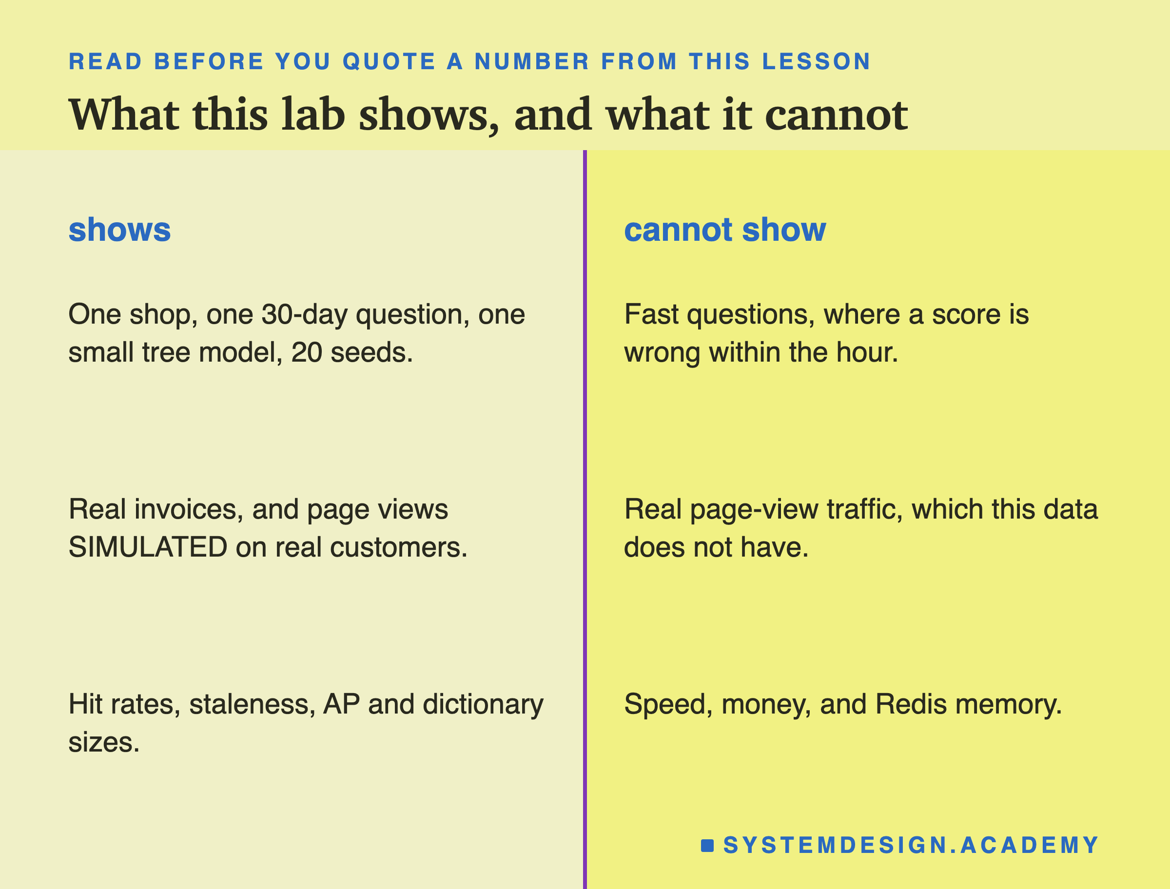
One shop, one slow question, one model. Everything here is one UK gift wholesaler, a 30-day question and lesson 1's visit-trained model. I make no claim about fast questions or other models.

The page views are made up. Their number, their sessions and their timing are my assumptions. Real browsing may cluster around orders, which would change the hit rates and the invalidation result. Five draws show the luck of the draw, not the luck of my assumptions.

By construction. On real invoices, "every hit is stale" and "invalidation means no hits" follow from the design. I counted them; they are not discoveries.

The bootstrap is a little optimistic. It redraws customers within each month, so the true intervals may be slightly wider.

No timings and no money. I did not time a cache hit or a model call on this busy laptop. Lesson 2 measured where the time in one request goes on a quiet machine.

Labelled additions. The checks on slides 14, 19 and 21 were done after the main results, and the direct comparison of dropping with keeping on slide 18 after an independent review. The lab labels each one.

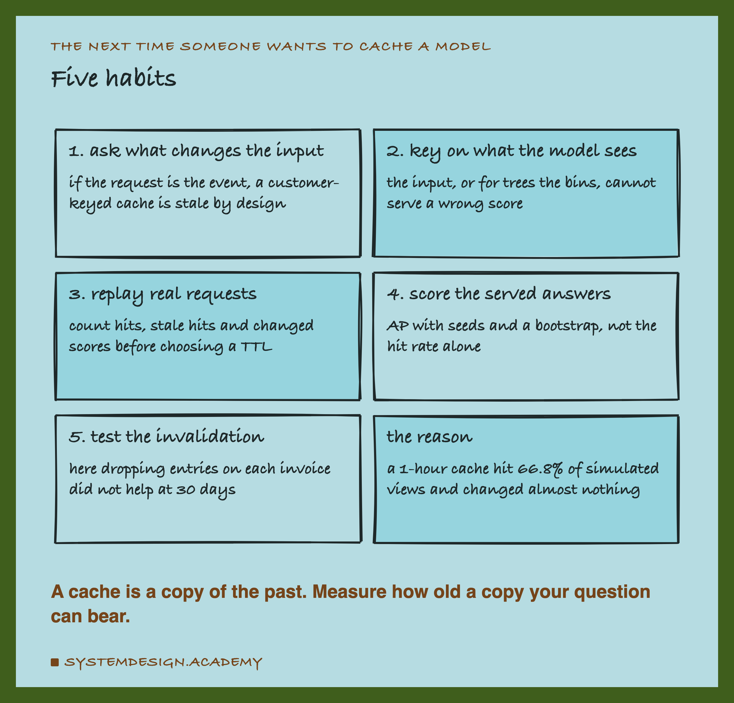
If someone on your team wants to put a cache in front of a model on Monday, do not start with the TTL. Start with your request log. Ask which requests change the inputs and which do not. Replay a week of real requests through two or three key choices and TTLs, and count the hits, the stale hits and the changed scores. Then score the served answers against fresh ones, with several seeds and a bootstrap.

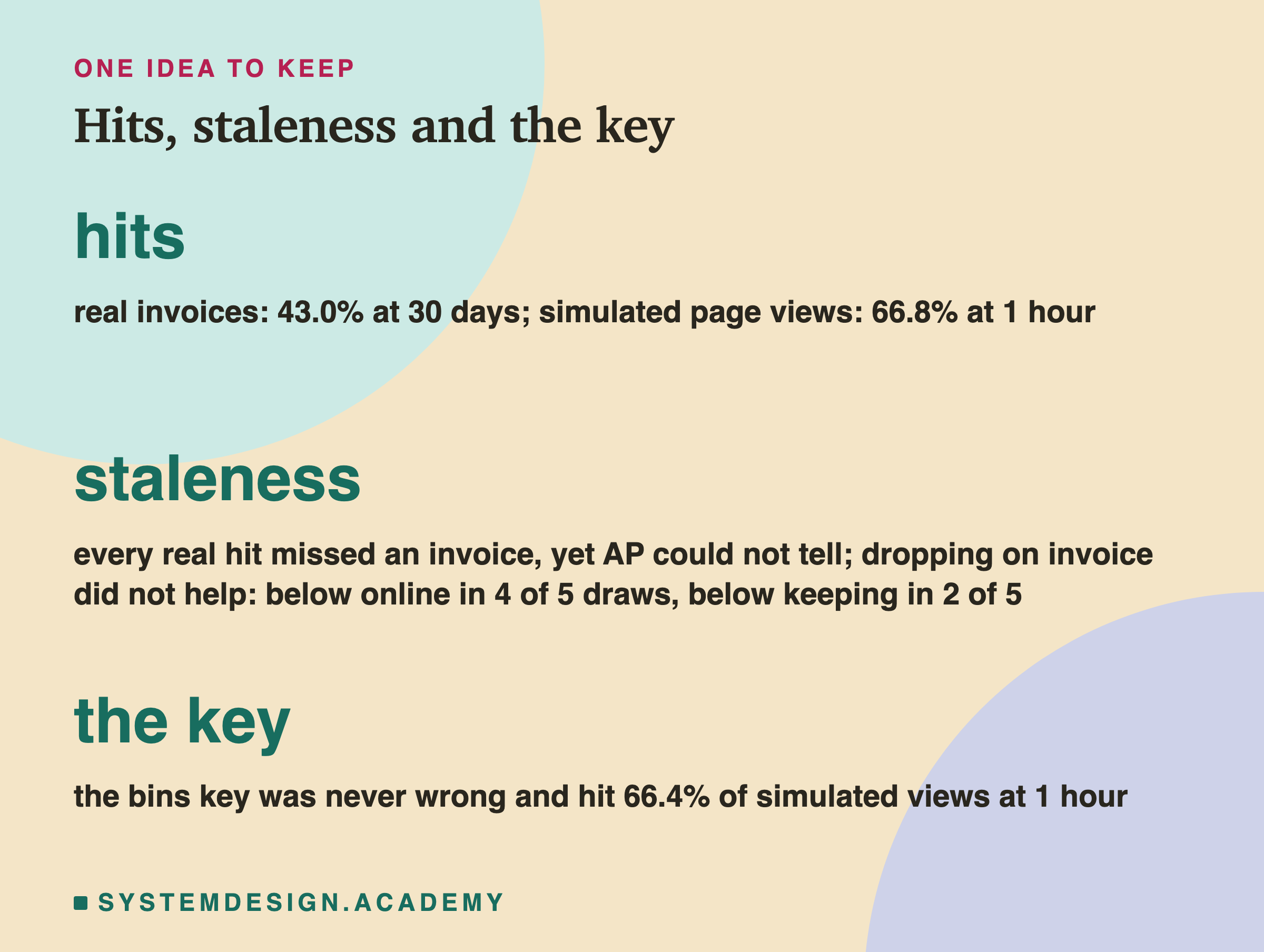
The one idea to keep: a cache is a jar of old answers, and three choices decide whether it helps. What the key is: here, a key built from the model's bins was never wrong. How long an entry lives: here, 1 hour on page views was almost free, and 30 days changed half the hits. And when entries die: here, dropping them on each invoice did not help. Measure all three on your own requests.