Let me start with a notebook and a library.

Imagine you help at a small club. For a year, you keep every member's record in your own notebook. Each night you write a new line for anyone who did something that day. The line says how many times they have visited so far, and how much they have paid so far. You date each line with the next morning, because that is when the line is finished.

When someone asks "how active was this member on 1 July?", you do not read the newest line. You turn back to the last line dated on or before 1 July. That way you never use what happened later.

Now a real library offers to keep the records for you. It has a proper catalogue, rules and staff. It says it can answer the same question for thousands of members at once. Before you hand over your notebook, you would want to check one thing. Does the library give the same answer as your notebook, for every member and every date? And are there any library rules you did not know about?

I do exactly this in this lesson. My notebook is the code I wrote in lessons 1 and 2. The library is a real feature store called Feast.

This is the last lesson of the chapter, so it leans on the earlier ones. If the shop, the customers or the question are new, please read what a feature is first. That lesson built six features from each customer's history: recency, frequency, money, return share, tenure and products. The question is always the same. At the start of a month, will this customer buy something in the next 30 days?

The most important earlier lesson here is point-in-time joins. It showed that joining each customer's latest values promised a score of 0.714 and delivered 0.301, and it wrote the correct join by hand with pandas' merge_asof. In this lesson I hand the same job to Feast and compare the two, row by row.

Three more lessons come back here. Feature freshness described how a feature store copies values to a fast store. Online and offline consistency compared two programs that compute the same feature. Missing at serving read in Feast's source code what happens to a customer the store does not know. Here I run it.

The survey lesson feature stores explains what a feature store is and why teams use one. I do not repeat it. This lesson only measures.

Please read this slide slowly if any word is new. Every slide after it uses these words.

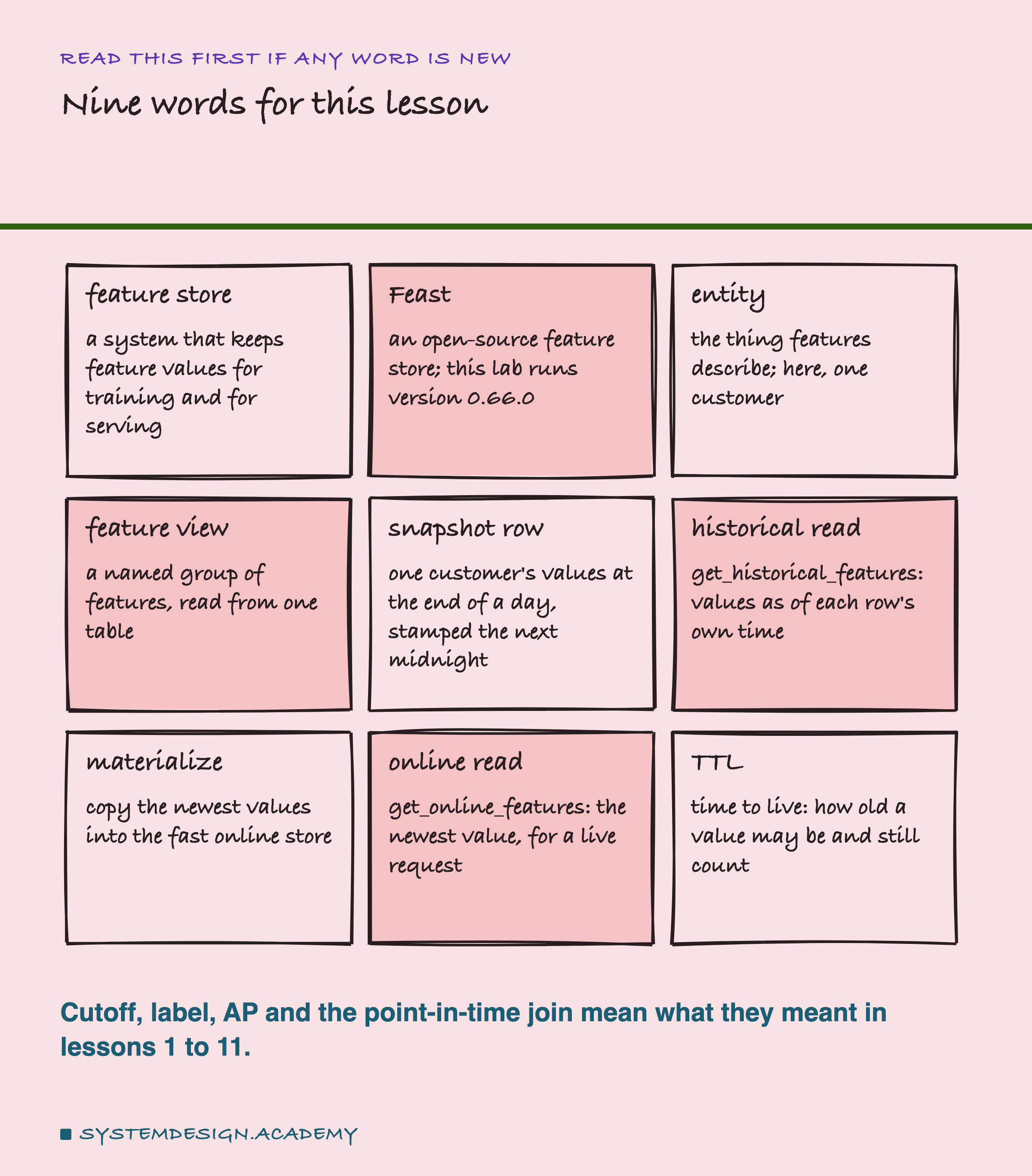
A feature store is a system that keeps feature values, both for building training data and for answering live requests. Feast is a popular open-source one. I use version 0.66.0, installed from the Python package index.

An entity is the thing the features describe. Here it is one customer, named by a customer number. A feature view is a named group of features that Feast reads from one table. A snapshot row is one customer's values at the end of one day. In my notebook story, it is one dated line.

The historical read is a Feast call named get_historical_features. You give it a list of rows, each with a customer and a time, and it returns the feature values as they were at each row's own time. To materialize means to copy the newest values into a small, fast store, called the online store. The online read, get_online_features, asks that fast store for the newest values, as a live service would. TTL means time to live: how old a value may be and still count.

Everything in this lesson ran on one laptop, with no server and no cloud account.

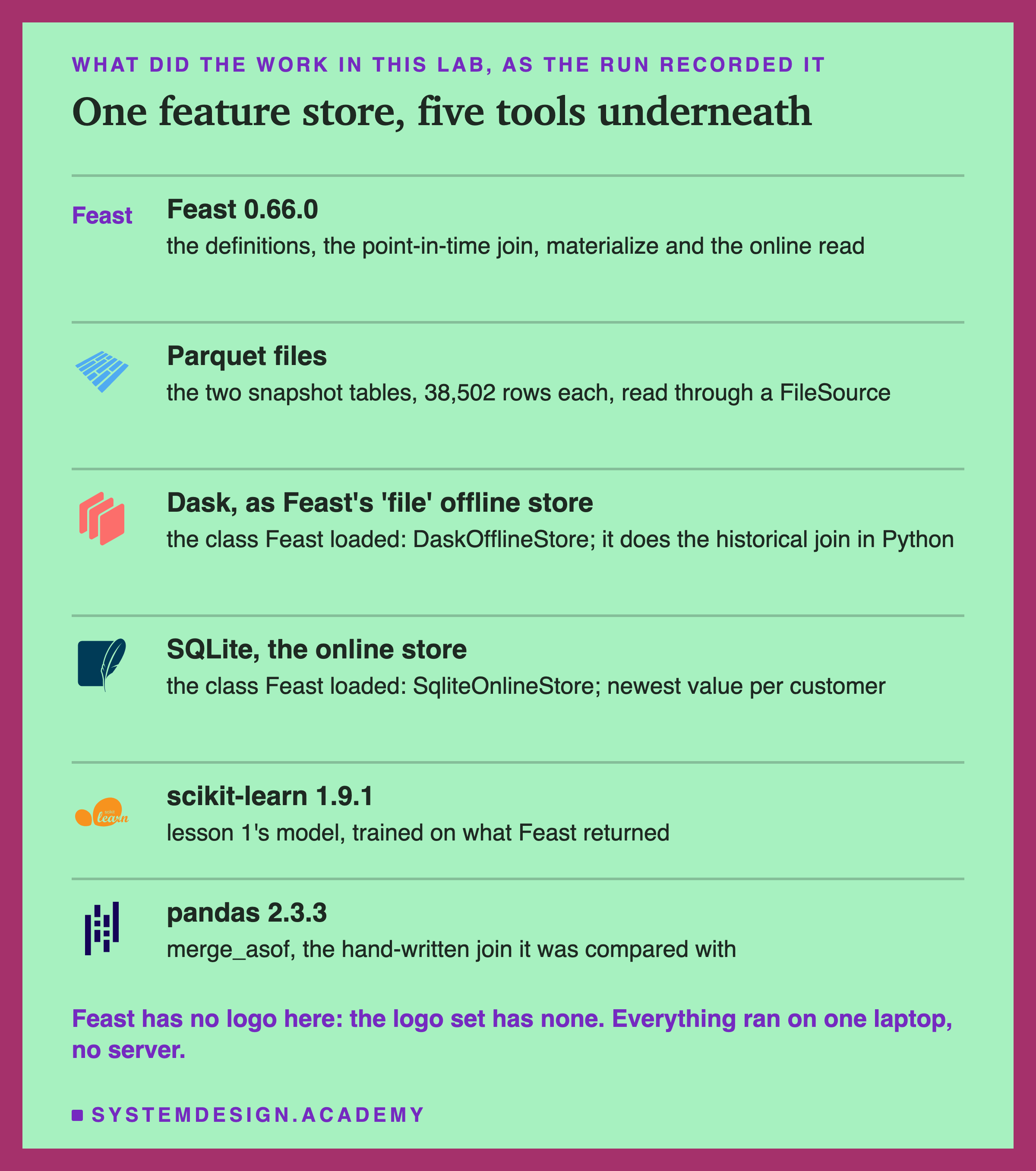
Feast does not do every job itself. When you tell it to read plain files, it uses a library called Dask to do the historical join in Python. Feast calls this the "file" offline store. The offline store is where the full history lives. For the online store I used SQLite, a small database that lives in one file. My tables were Parquet files, a common file format for tables. The lab recorded which classes Feast actually loaded, so these are not guesses.

Feast needed its own Python environment. A virtual environment is a separate folder of Python packages, so two projects cannot break each other. Feast 0.66.0 requires pandas older than version 3, while the rest of this chapter used pandas 3.0.6. Feast's own tests run on Python 3.10, 3.11 and 3.12, so I used Python 3.12.14. The lab saved the exact list of every package and version into its results file.

Feast's own page for the Dask store warns that it "may not scale to production workloads". It is meant for trying Feast on one machine, which is what I did.

Here is the path a feature value takes in this lab, with the Feast calls I made.

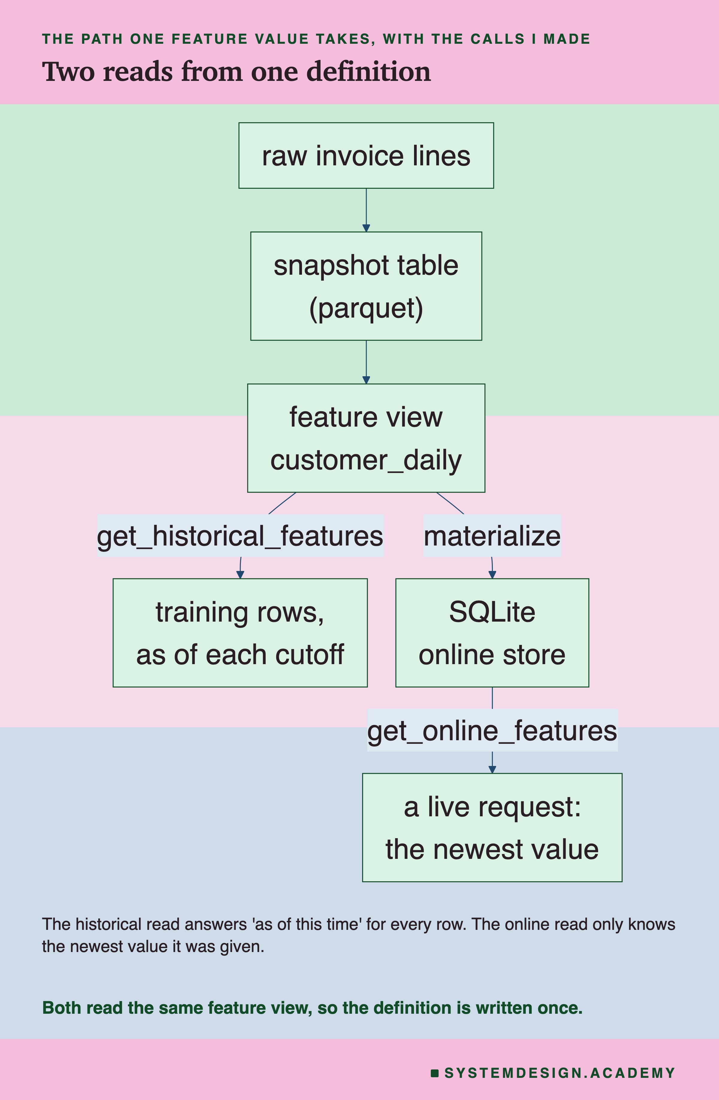
I built the snapshot table from the raw invoice lines myself, with pandas, and wrote it to a Parquet file. Feast does not compute these running totals for me. I only told Feast where the file is, which column is the customer and which column is the time.

From there, two reads use the same feature view. The historical read builds training rows: for each customer and each cutoff, the values as they were at that cutoff. The online read serves a live request: for each customer, the newest value that was copied in.

This split is the main promise of a feature store. You describe the features once, and both training and serving read from that one description. The survey lesson explains why that matters. My job here is to check that the historical read really is a correct point-in-time join.

Feast needs a table with a time column. I built it the way a nightly batch job would, the same way as lesson 2.

For every customer, and every calendar day on which that customer has at least one invoice line, the table has one row. The row holds running values up to the end of that day. They are the time of the first line and of the last line, the number of purchase invoices, and the net money. It also holds the share of lines that were returns, and the number of different products bought. The row is stamped at the next midnight, because that is the moment the night's job has seen the whole day.

Recency and tenure change every day, even when nothing happens. So I did not store them. I stored the times of the first and last lines instead. After the join, I computed recency as the cutoff minus the last line, in days. Tenure is the cutoff minus the first line. Lesson 1 computes them the same way. The table has 38,502 rows for 5,942 customers.

These are the definitions I gave Feast. They live in scripts/labs/features/feast_repo/definitions.py, next to a short feature_store.yaml that names the SQLite online store and the file offline store.

"""Lesson 12 of 'Features and Feature Stores': what Feast is told about the data (Feast 0.66.0).

One entity (a customer) and three feature views over two parquet snapshot tables that feast_lab.py writes to
$FEAST_DATA (default ~/lab-data/features/feast-repo):

  customer_daily.parquet  lesson 1's six features, as running totals. One row per customer per calendar day
                          on which they have any invoice line, stamped at the NEXT midnight (the moment a nightly
                          job has seen the whole day). Two date columns are stored as whole seconds since
                          1970-01-01 so recency and tenure can be worked out at any cutoff after the join.
  customer_l2.parquet     lesson 2's feature table, unchanged (point_in_time.feature_table), same stamps.

ttl = timedelta(0) means "no limit": Feast looks back as far as the table goes. customer_daily_ttl90 is the same
table with a 90-day TTL, to see what TTL does.

Author: Roni Das
Created: 2026-10-01
"""
import os
from datetime import timedelta
from pathlib import Path

from feast import Entity, FeatureView, Field, FileSource
from feast.types import Float64, Int64
from feast.value_type import ValueType

DATA = Path(os.environ.get("FEAST_DATA", Path.home() / "lab-data" / "features" / "feast-repo"))

customer = Entity(name="customer", join_keys=["customer_id"], value_type=ValueType.INT64,
                  description="One shop customer (CustomerID in UCI Online Retail II)")

daily_source = FileSource(name="customer_daily_source", path=str(DATA / "customer_daily.parquet"),
                          timestamp_field="feature_ts")
l2_source = FileSource(name="customer_l2_source", path=str(DATA / "customer_l2.parquet"),
                       timestamp_field="feature_ts")

DAILY_FIELDS = [
    Field(name="snap_unix", dtype=Int64),          # the row's own stamp, so I can see WHICH row was joined
    Field(name="first_event_unix", dtype=Int64),   # first invoice line so far -> tenure_days
    Field(name="last_event_unix", dtype=Int64),    # last invoice line so far -> recency_days
    Field(name="frequency", dtype=Int64),          # distinct purchase invoices so far
    Field(name="money", dtype=Float64),            # net spend so far, returns included (negative)
    Field(name="return_share", dtype=Float64),     # return lines / all lines so far
    Field(name="products", dtype=Int64),           # distinct stock codes on purchase lines so far
]

customer_daily = FeatureView(name="customer_daily", entities=[customer], ttl=timedelta(0),
                             schema=DAILY_FIELDS, source=daily_source, online=True)

customer_daily_ttl90 = FeatureView(name="customer_daily_ttl90", entities=[customer], ttl=timedelta(days=90),
                                   schema=DAILY_FIELDS, source=daily_source, online=True)

customer_l2 = FeatureView(
    name="customer_l2", entities=[customer], ttl=timedelta(0), source=l2_source, online=False,
    schema=[Field(name="snap_unix", dtype=Int64), Field(name="frequency", dtype=Int64),
            Field(name="money", dtype=Float64), Field(name="return_share", dtype=Float64),
            Field(name="last_buy_unix", dtype=Float64)])   # empty (NaN) while a customer has only returned

OBJECTS = [customer, daily_source, l2_source, customer_daily, customer_daily_ttl90, customer_l2]

Here is one real customer, number 12395, and three of their 17 snapshot rows.

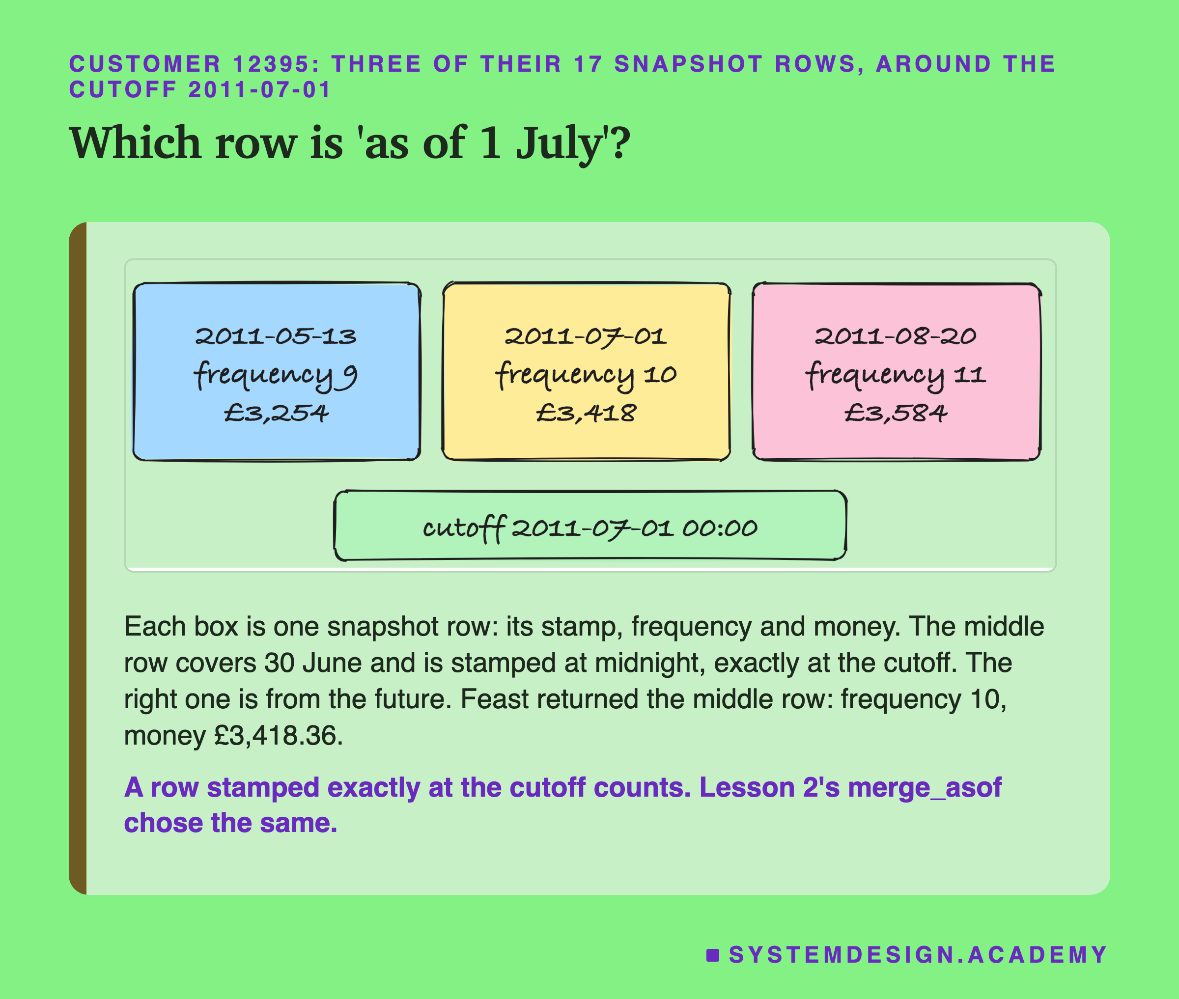
This customer bought something on 30 June 2011. The nightly job wrote a row for that day and stamped it at midnight, which is 00:00 on 1 July. The cutoff is also 00:00 on 1 July. So the row's stamp and the cutoff are exactly the same moment.

Should the join take that row? Yes. It covers 30 June, so it holds nothing from 1 July onward. It is the freshest row that is still legal. Lesson 2 thought about this carefully, and chose allow_exact_matches=True in merge_asof so that a row stamped exactly at the cutoff counts.

The row on the right, stamped 20 August, is from the future and must never be used for a 1 July cutoff. Feast returned the middle row: frequency 10 and money £3,418.36. Recency came out as 0.297 days, about seven hours, because the last line on 30 June was at 16:52.

Before running anything, I read how Feast's file store does the join. I cloned Feast's code at the tag for version 0.66.0, commit 1d5be950, and read the file dask.py. Every quote is in results/feast-factcheck.json, with the line numbers.

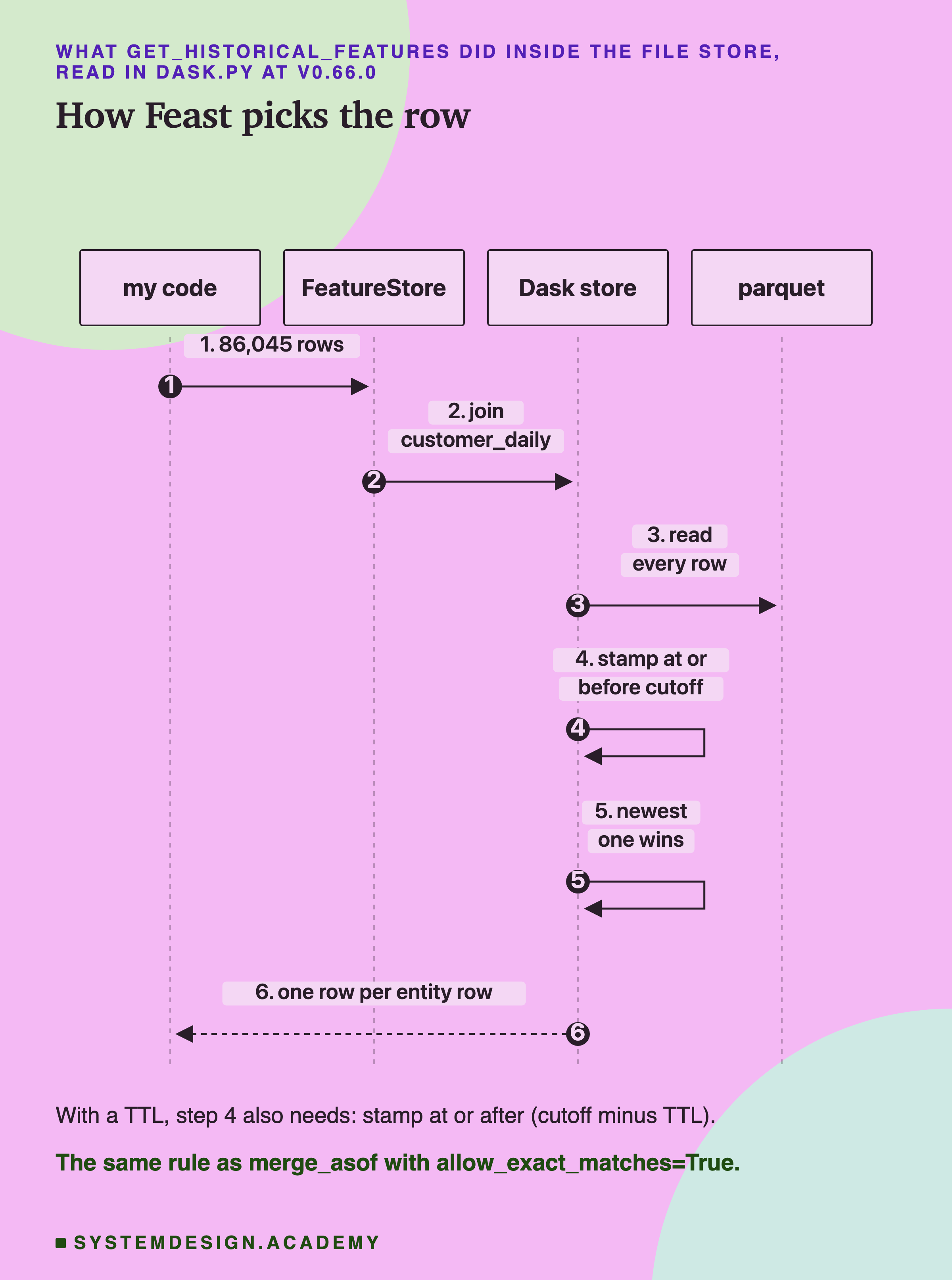
The code does three things. First it joins every one of a customer's snapshot rows onto each of that customer's entity rows. An entity row is one row of the list I hand to Feast: a customer and a time. Then it keeps only the snapshot rows whose stamp is less than or equal to the entity row's time. The code says <=, and Feast's documentation says the time is the "upper bound (inclusive)". Then it sorts by stamp and keeps the newest one.

With a TTL, there is one more condition. The stamp must also be at or after the entity time minus the TTL. A TTL of zero means no limit. Feast's own description says a TTL of 0 means the features live "forever". And Feast treats a time with no time zone as UTC, on both sides of the join, so my plain shop times did not shift.

One more detail mattered later. The step that keeps rows only lets through rows inside the time window, or rows where the customer had no snapshot at all. So a customer who has snapshots, but none inside the window, is left with nothing. I wrote in the lab's design, before it ran, what I expected that to do to rows outside a TTL. After an independent review, I also checked rows from before a customer's first snapshot. The slide on TTL shows both.

I wrote the lab's design into the docstring of scripts/labs/features/feast_lab.py before it first ran. I had read Feast's code first, as the last slide says, but no Feast call had run on this data.

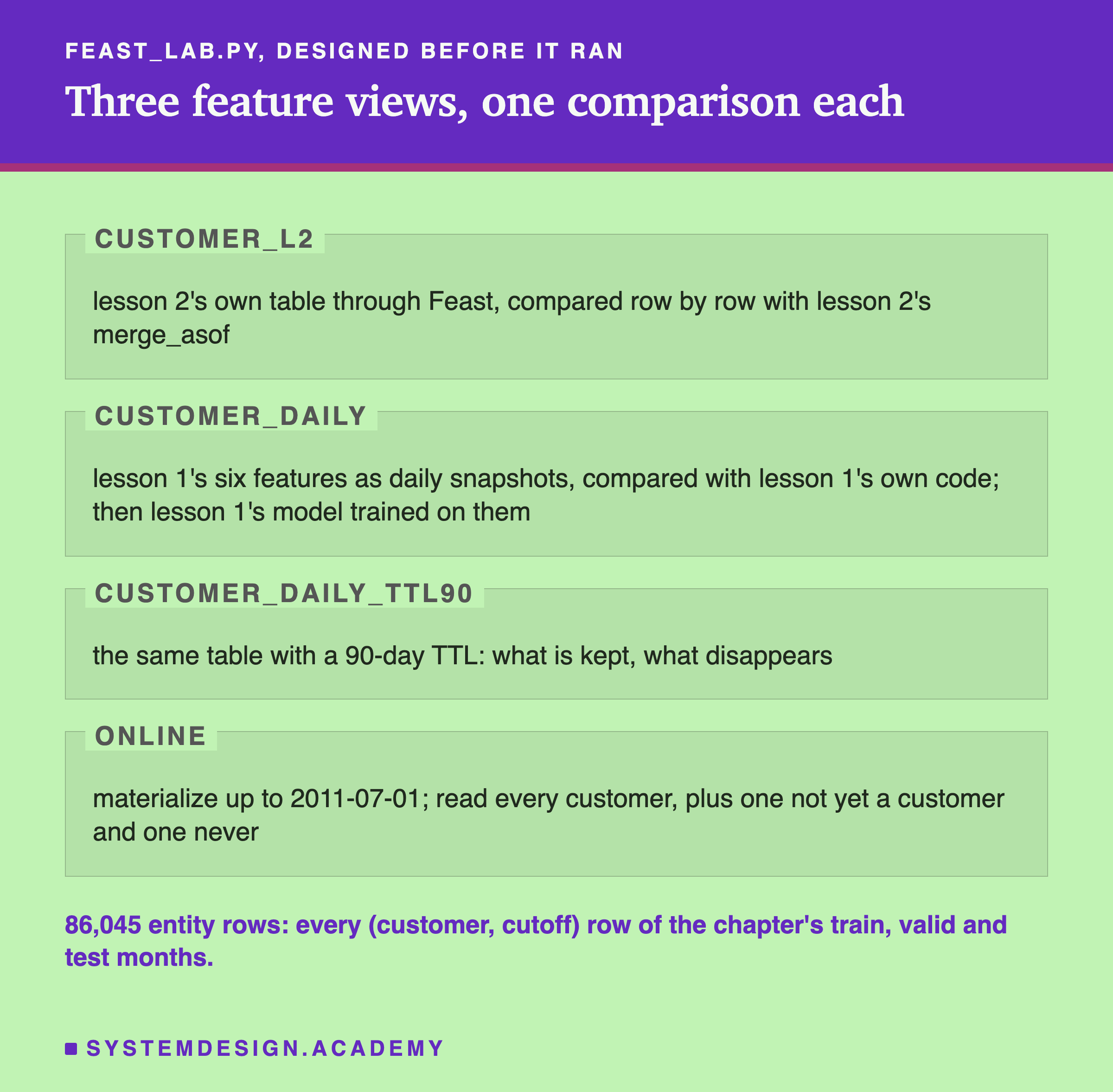
The rows. I asked Feast for every row the chapter uses: 44,521 training rows, 14,673 validation rows and 26,851 test rows, 86,045 in all. Each row is a customer and a cutoff, the first of a month, as in every lesson.

Three feature views. The first, customer_l2, is lesson 2's own table. I compared Feast's answer with lesson 2's merge_asof on every row and every column. The second, customer_daily, holds lesson 1's six features. I compared it with lesson 1's own code, rebuilt in the same environment, and then trained lesson 1's model on Feast's columns. The third, customer_daily_ttl90, is the same table with a TTL of 90 days.

Equal means equal. A row matches only if every value is identical, to the last bit, with two empty values counted as equal. I did not allow a tolerance, so any difference in how a number was added up would show.

The model is the chapter's own: scikit-learn's HistGradientBoostingClassifier with its default settings and seed 0, trained on the training months and scored by average precision (AP) on the five test months. Lesson 1 stored a test AP of 0.5450 for it.

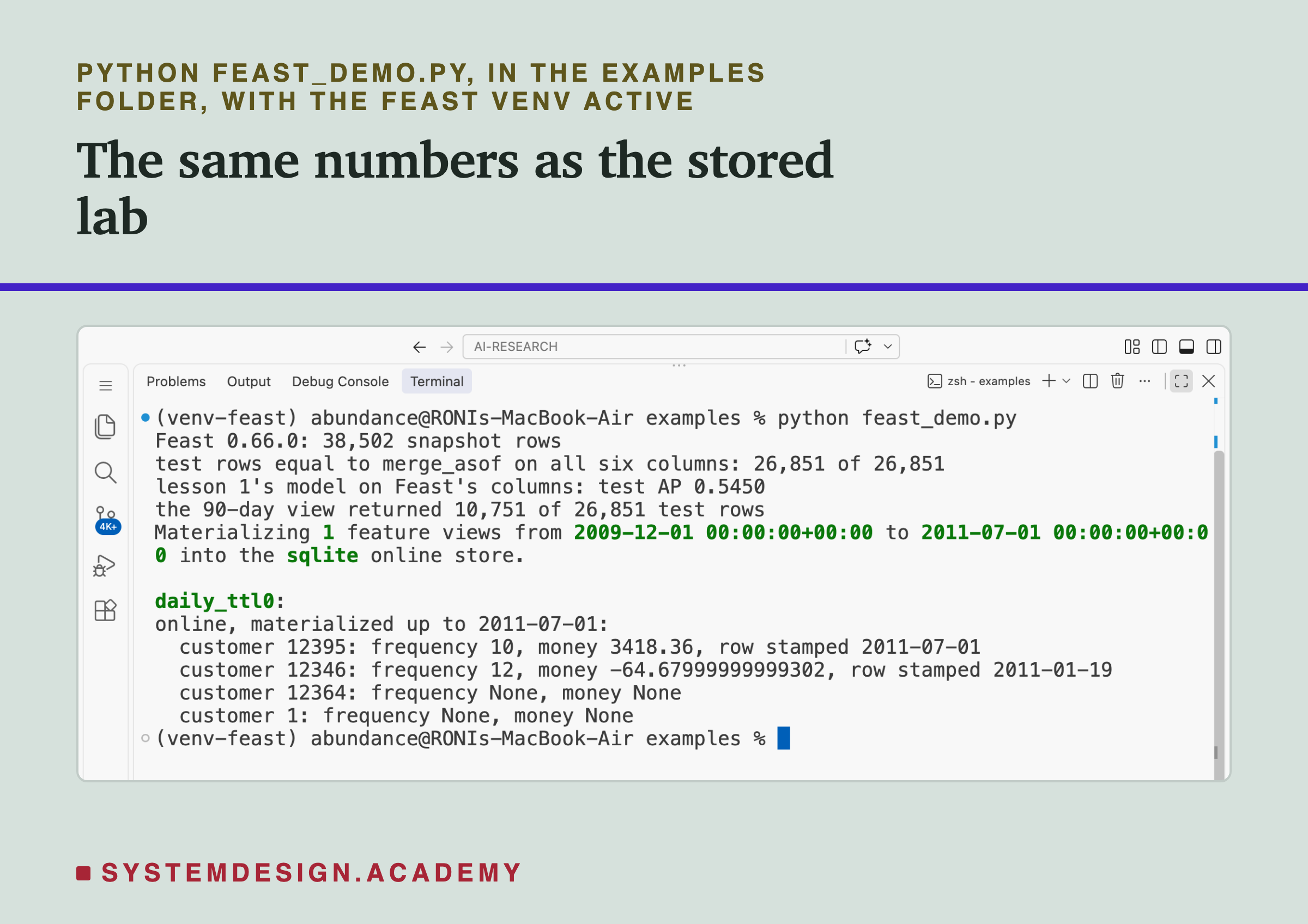
This is a real recording of the report script, feast_report.py, on the laptop where the lab ran, inside the Feast environment.

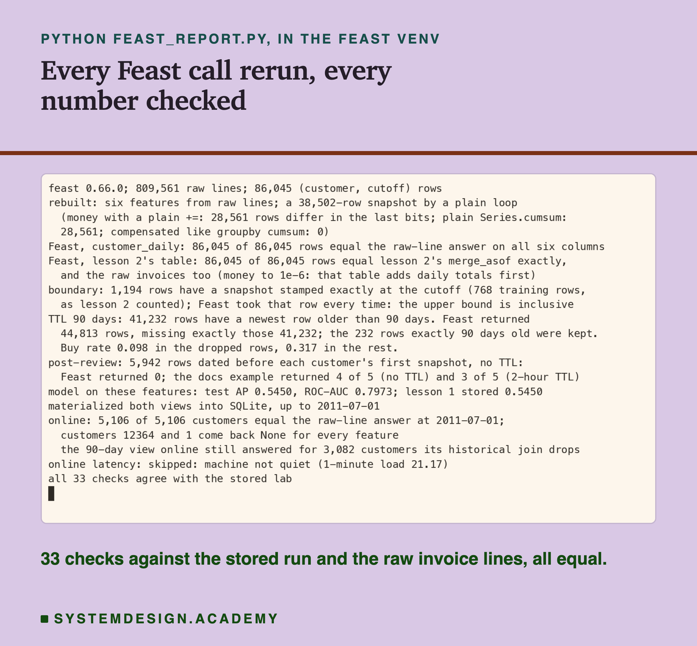
The report does not reuse the lab's code for the parts that matter. It computes lesson 1's six features straight from the raw invoice lines, for every customer and cutoff, with no snapshot table and no join. A correct point-in-time join must give this answer. Then it builds a new snapshot table with a plain Python loop, puts it into a brand new Feast store in a temporary folder, and asks Feast again.

Feast's answer from that new store must equal the raw-line answer on every row. The report also rechecks lesson 2's table, the TTL counts, the model's score and the online answers. If any number differs from the stored run, it stops with an error. It ran 33 checks, including the two added after the review, and all of them agreed.

Here is the main result. With no TTL, the historical read of Feast's file store gave exactly the same answer as my hand-written joins.

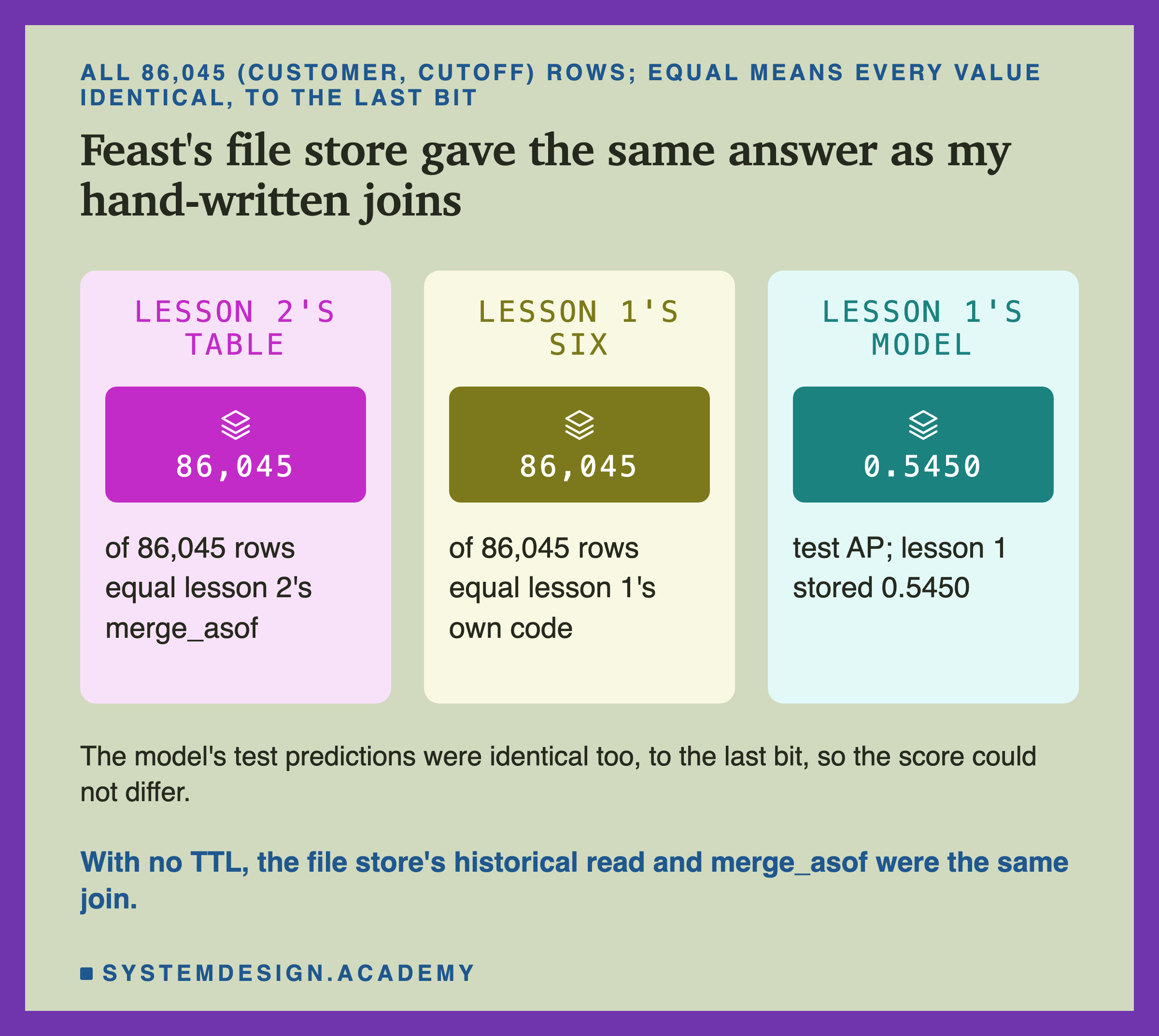
Lesson 2's table through Feast equalled lesson 2's merge_asof on 86,045 of 86,045 rows. Every column matched to the last bit: the joined row's stamp, frequency, money, return share, the last purchase time, and the recency computed from it.

Lesson 1's six features through Feast equalled lesson 1's own code on 86,045 of 86,045 rows, on all six columns. Lesson 1's code never builds a snapshot table. It adds up every line before each cutoff, directly. So this checks the whole path at once: my snapshot table, Feast's join, and the recency and tenure I computed after it.

Lesson 1's model, trained on Feast's columns, scored a test AP of 0.5450 and a ROC-AUC of 0.7973. Lesson 1 stored 0.5450. This match was not luck. The model's test predictions were identical to the last bit, so the score could not differ. With the same inputs in the same order, the same model gives the same answer.

So the answer to this lesson's question is yes. On this data, with no TTL, the historical read of Feast's file store is the point-in-time join that lesson 2 wrote by hand. One condition holds on every row here: each customer has a snapshot at or before the cutoff. The TTL slide shows what happens when that fails. A feature store does not add a different join. It adds two things: you no longer write the join yourself, and training and serving read one description.

The most delicate part of a point-in-time join is a row stamped exactly at the cutoff. Here is how often it happened.

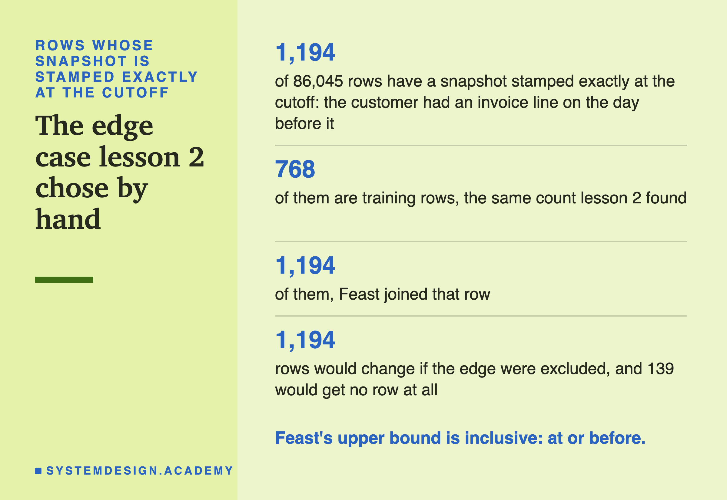
In 1,194 of the 86,045 rows, the customer had an invoice line on the last day before the cutoff, so their newest snapshot is stamped exactly at the cutoff. 768 of those are training rows. Lesson 2 counted the same 768, which the report checks. Feast took that row in all 1,194 cases.

If the edge had been excluded, as allow_exact_matches=False would do, all 1,194 rows would have changed. 139 of them would have had no row at all, because that day was the customer's first. So the difference between "before" and "at or before" matters here. It touches about one row in 72.

Feast's documentation says the entity time is an inclusive upper bound, and the file store's code says <=. My run agrees with both. That only matters because my rows mean "valid from midnight". If your stamps mean the time of the event itself, an inclusive bound could let an event at the cutoff leak in, and lesson 2's advice applies.

Now the library rule I did not know well enough: the TTL. I set the third feature view to a TTL of 90 days and asked for the same 86,045 rows.

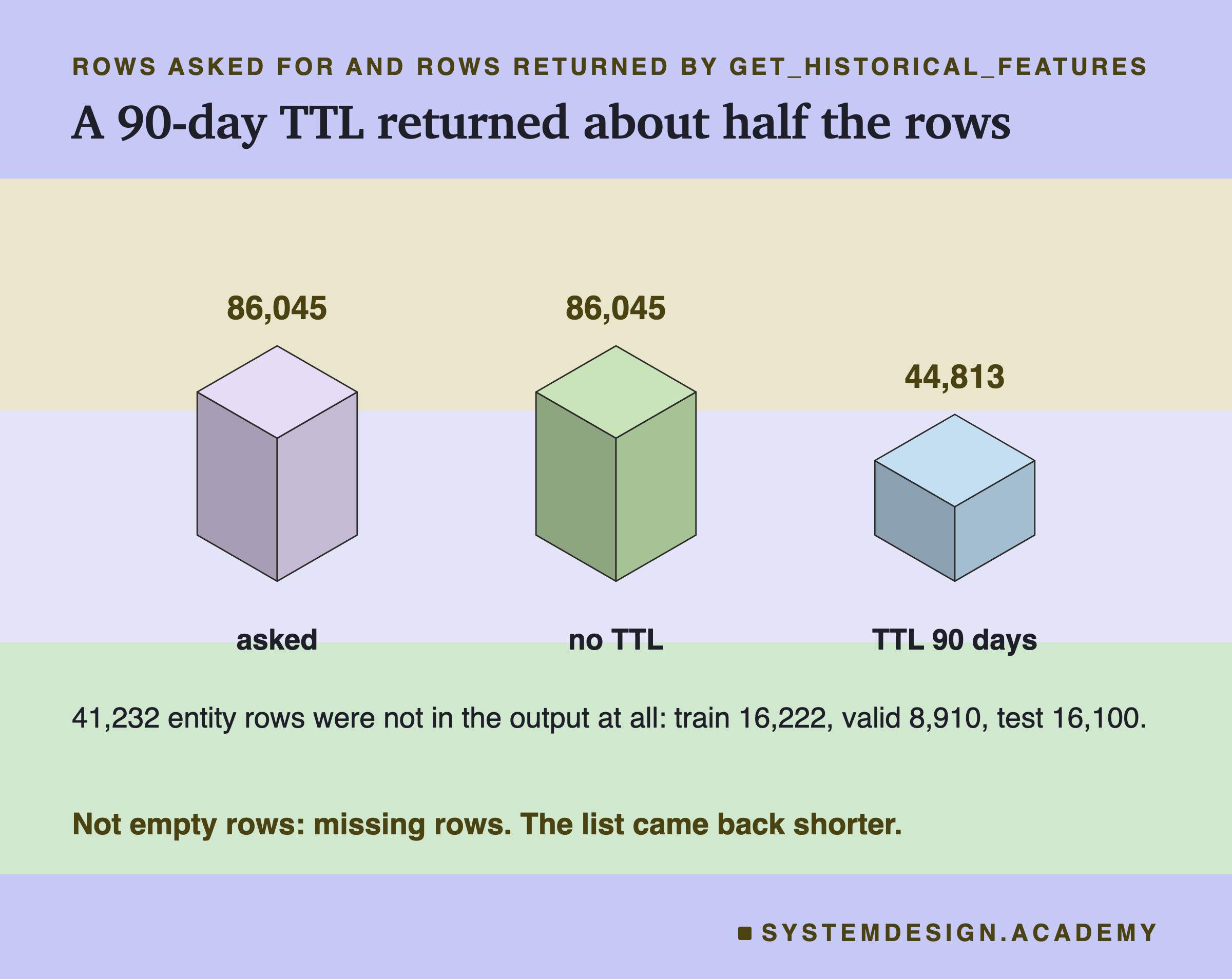
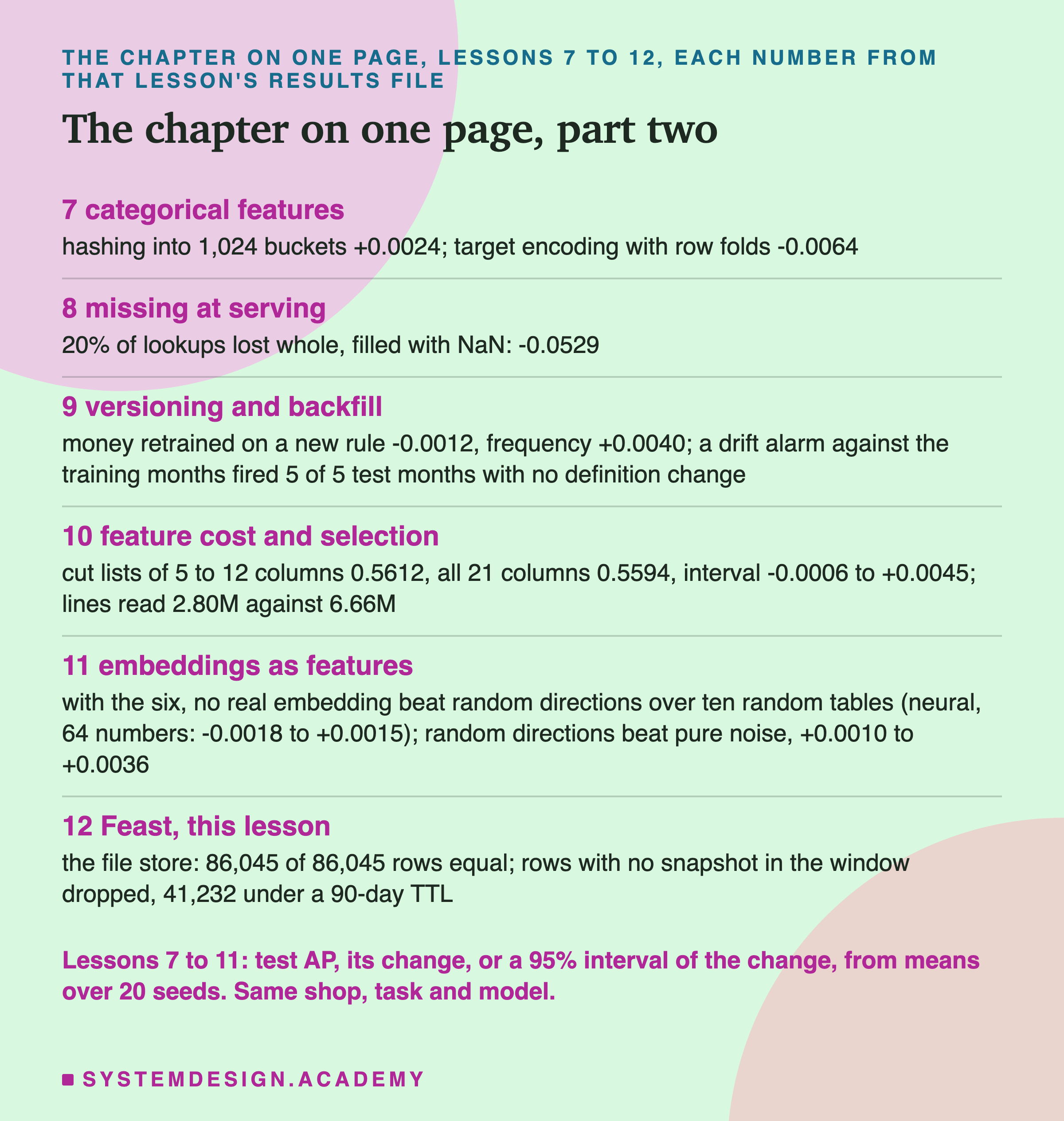
Without a TTL, Feast's file store returned all 86,045 rows. With a 90-day TTL, it returned 44,813. The other 41,232 entity rows were not returned with empty features. They were missing from the output altogether. My list of rows went in with 86,045 entries and came back with 44,813, with no error or warning printed. A program that does not count the rows would simply train on fewer customers and never know.

The dropped rows were exactly the ones the rule predicts: rows whose newest snapshot was more than 90 days older than the cutoff. The report computed that set from the raw lines and checked that it equals the missing set, row for row. The 232 rows whose newest snapshot was exactly 90 days old were kept, so the lower bound is inclusive too. Every row that came back was identical to the answer with no TTL.

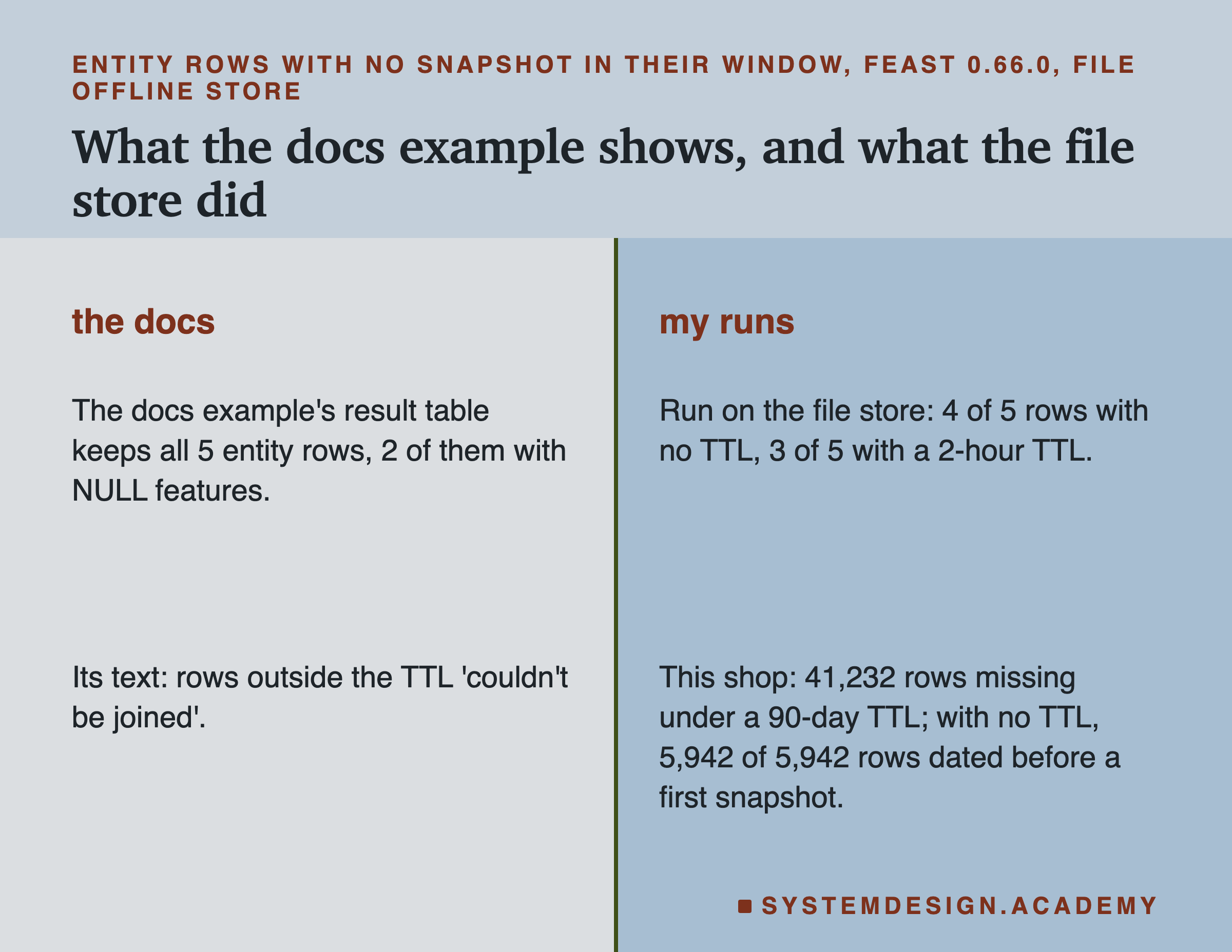
Feast's page on point-in-time joins shows a small example with one driver and five requests. Its text says a row outside the TTL "couldn't be joined". Its picture of the result keeps all five entity rows, two of them with NULL, meaning empty, features. The file store at version 0.66.0 does not do that. It drops the row. I expected this from reading its code, and wrote the guess down before the run. The left join brings in all of a customer's snapshot rows. The time filter then removes every one of them, so nothing is left to carry the entity row through.

The TTL is not the only cause. An independent review pointed out that the same filter also removes snapshot rows stamped after the entity time. I added a check to the lab after the review, and it is labelled there. The file store drops any entity row whose customer has snapshots but none in the window. The snapshots are either older than the TTL, or, with no TTL, only newer than the cutoff. The no-TTL run lost nothing only because every row in this chapter has history before its cutoff.

A TTL of 90 days sounds generous. Why did it drop almost half the rows?

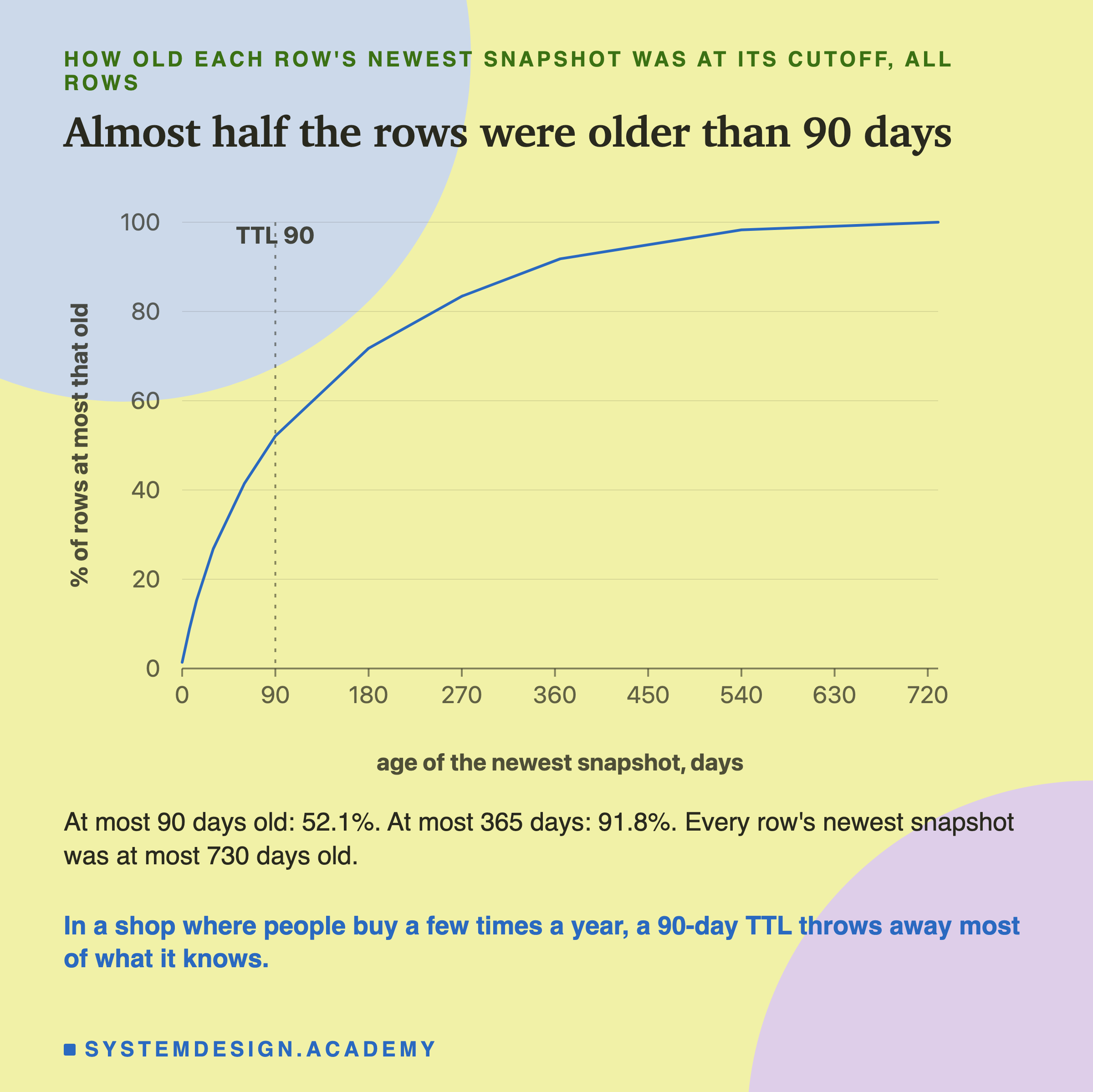
The chart shows how old each row's newest snapshot was at its cutoff. I added it to the report after seeing the results, as a description of the data. Only 52.1 percent of rows had a snapshot at most 90 days old. In this shop, many customers buy a few times a year, or once and never again. Their newest row is old, but it is still true: it is still everything they have done.

A TTL is meant for values that go stale, like a sensor reading or a price. A running total over a customer's whole history does not go stale. A customer who last bought 200 days ago still bought 12 times in total. For features like these, a TTL deletes good information.

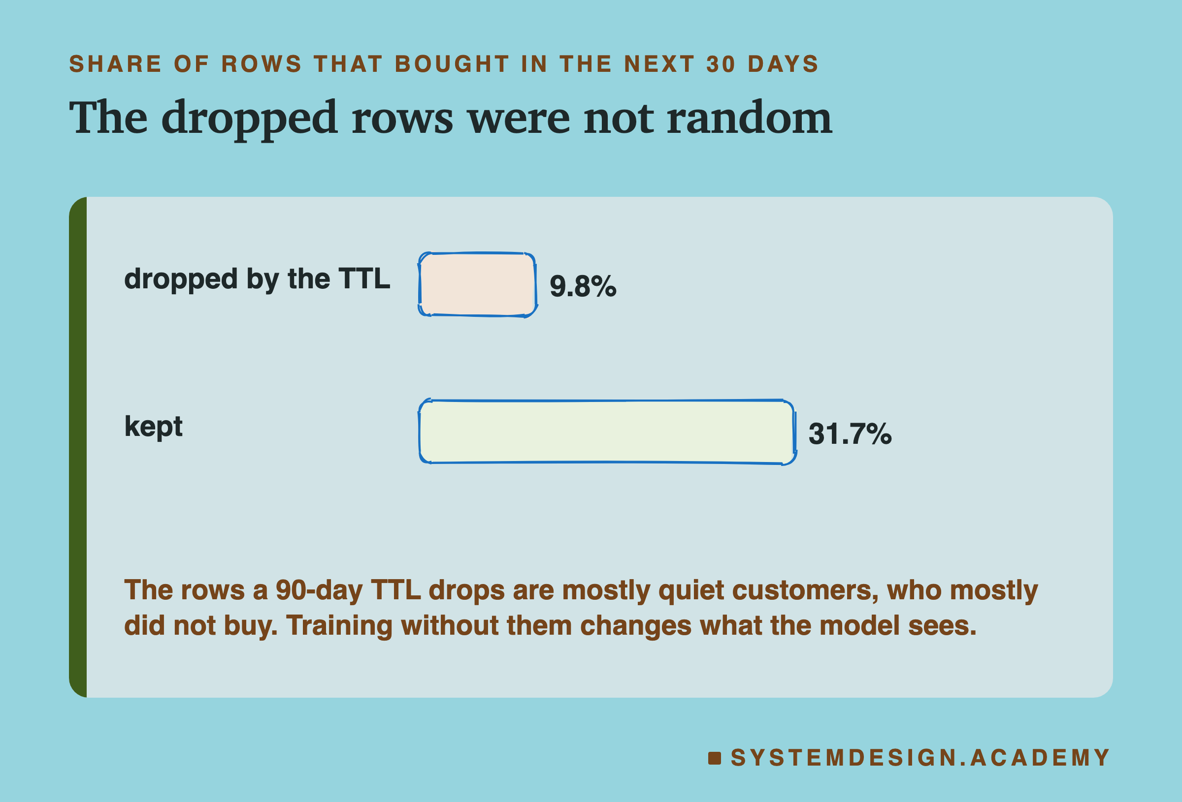
The dropped rows are also not random. Of the dropped rows, 9.8 percent bought in the next 30 days. Of the rows kept, 31.7 percent did. A training set built with this TTL would hold far fewer quiet customers, and its buy rate would look much higher than the shop's. I did not train a model on it, so I cannot say what score it would get. I can only say the training rows would be a different, biased set.

Next, the online side. I ran materialize from 1 December 2009 to 1 July 2011 into the SQLite online store, and then asked it about customers.

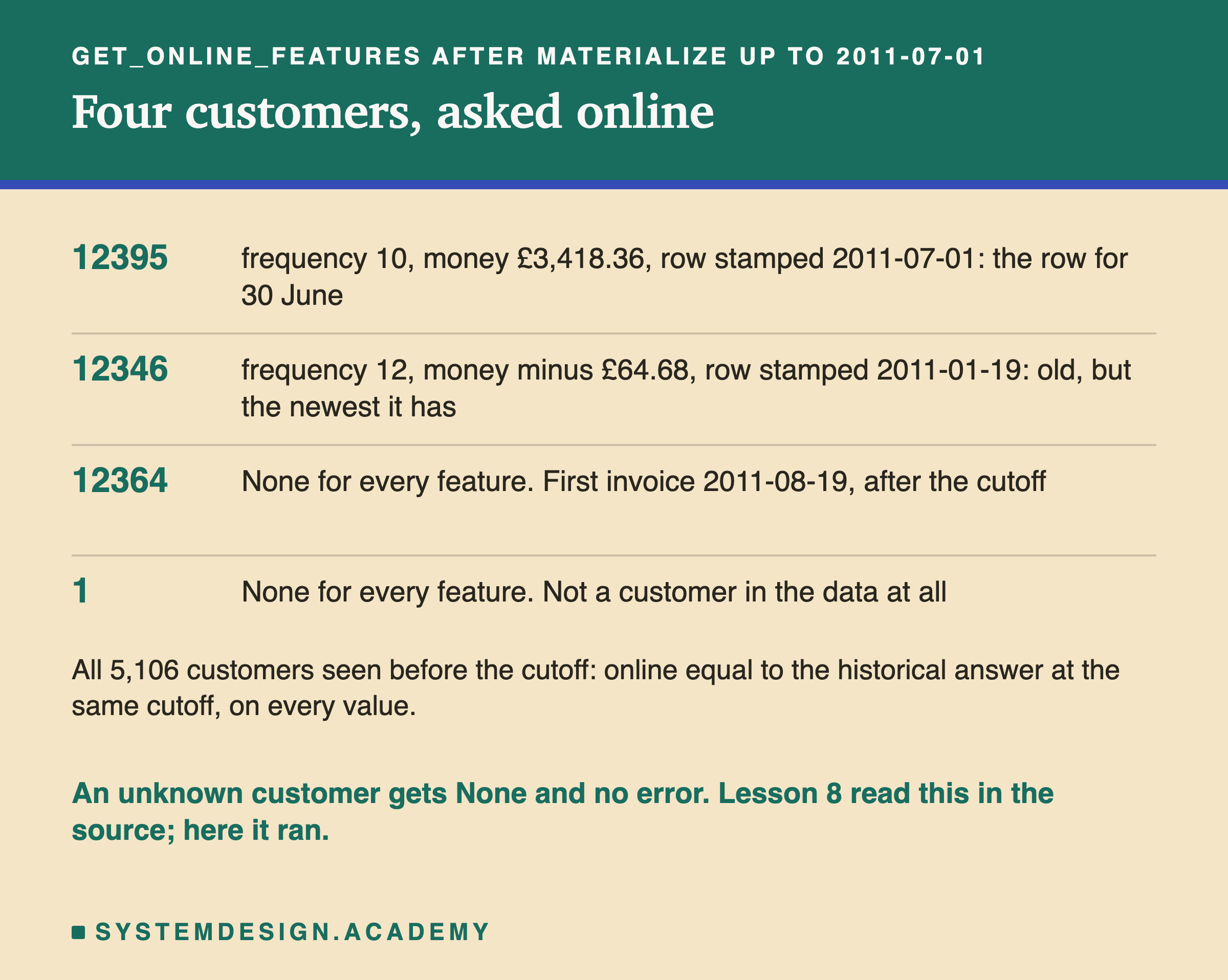
The online store keeps only the newest value for each customer. Feast's documentation says so, and the code's materialize step keeps the newest row in the time window. The window included its end, 00:00 on 1 July, so customer 12395 got the row for 30 June, the same row the historical read chose.

I asked for all 5,106 customers seen before 1 July 2011. Every one of them got exactly the same seven values online as the historical read gave at that cutoff. So online and offline agreed. Lesson 5 found that two separate programs did not quite agree; here it holds because one program wrote both sides.

Then I asked about two customers the store cannot know. Customer 12364 first appears in the data on 19 August 2011, after the end of the copied window. Customer 1 does not exist in the data. Both came back with None for every feature, and an event time of zero. There was no error and no warning. Lesson 8 read this behaviour in Feast's source. Now I have seen it run. Your serving code must check for None itself, and lesson 8 measured what each way of filling the gap costs.

Then I asked the 90-day view online, for the same 5,106 customers.

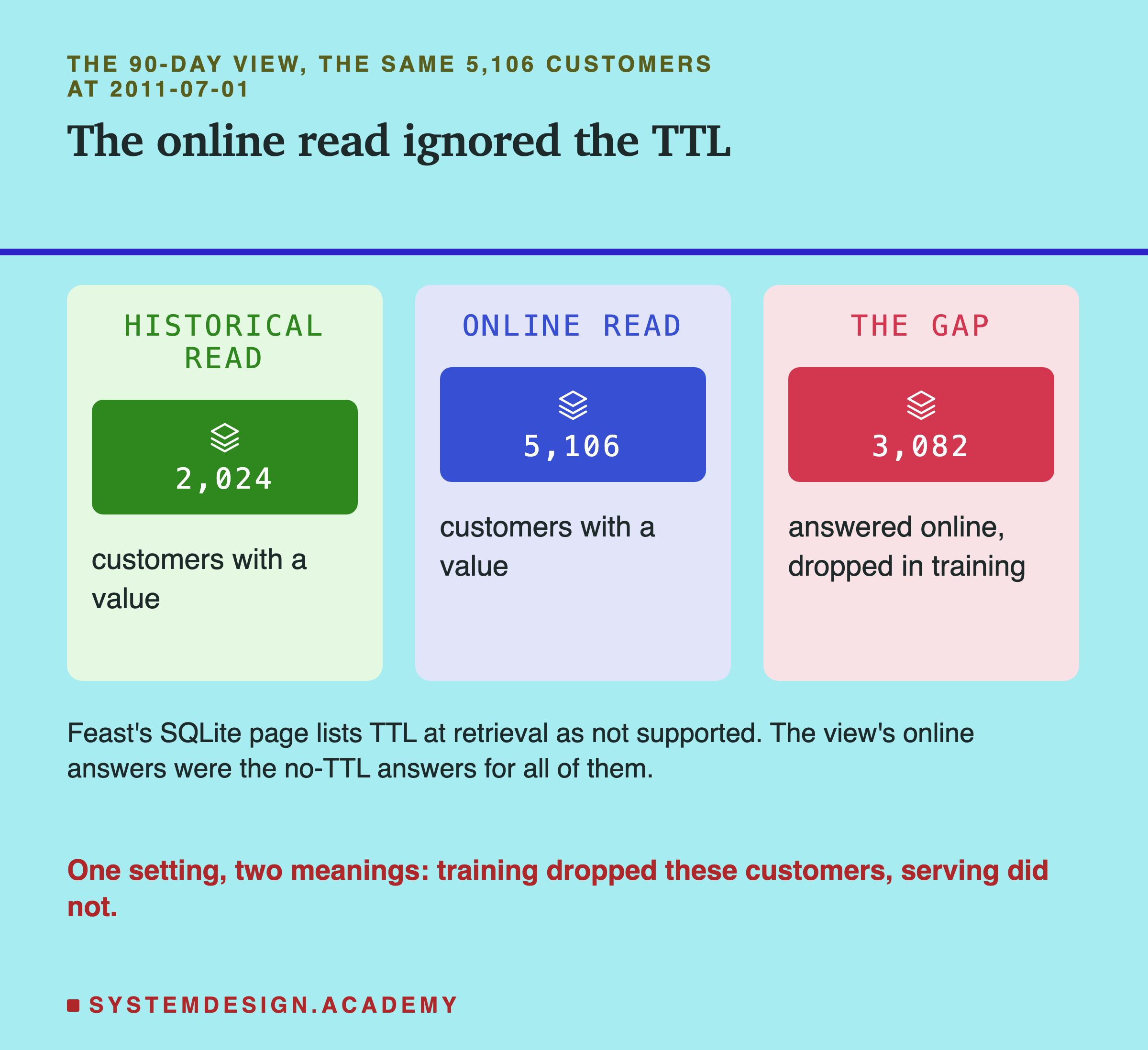
At the 1 July cutoff, the historical read with a 90-day TTL had values for only 2,024 of these customers. The online read of the same view answered for all 5,106. For 3,082 customers, the store served a value online that the same view's historical read would have dropped from training. The online answers were identical to the view with no TTL.

Feast's own page for the SQLite online store has a table of features, and one row says "support for ttl (time to live) at retrieval: no". So this is documented. But a general page about feature retrieval says event times are used "to ensure that old feature values aren't served to models during online serving". For SQLite in version 0.66.0, that did not happen in my run.

So one setting meant two different things. In training, the TTL removed these customers. In serving, it did nothing. A model trained with this view would never see a customer whose newest row is older than 90 days. Then, at serving, it would be asked about thousands of them. This is exactly the kind of training and serving mismatch that lesson 5 measured, made here by a single setting.

One result surprised me: money matched lesson 1 exactly, on every row. Money is a sum of many decimal amounts, and lesson 5 showed that two ways of adding the same amounts can differ in the last digits.

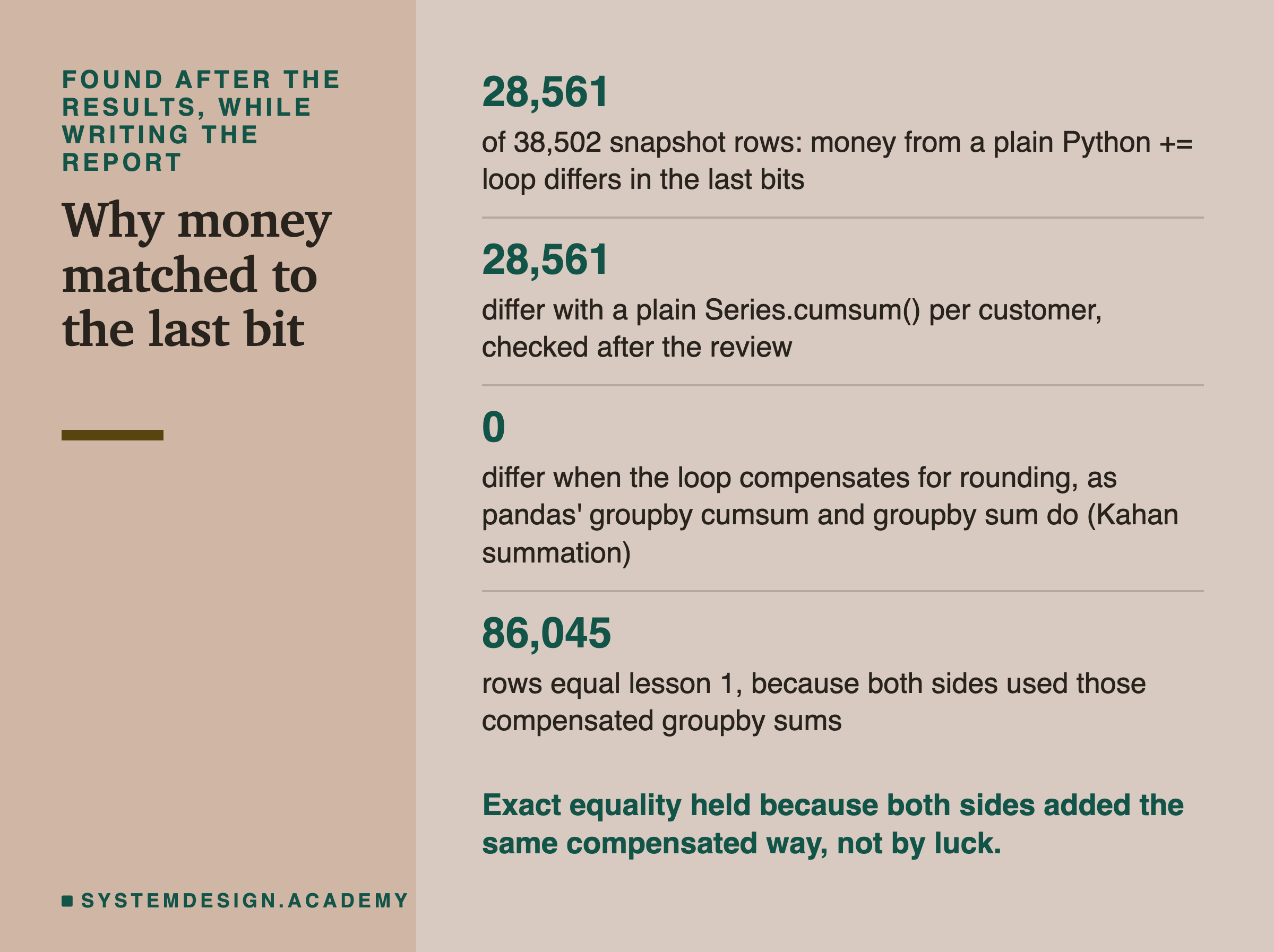
I found the reason after the results, while writing the report, and the report labels it so. My first version of the report built the snapshot table with a plain Python loop that added each amount with +=. Its money differed from the lab's table in the last bits on 28,561 of 38,502 rows, and the report stopped.

The lab built its table with pandas' groupby running sum, a groupby cumsum, and lesson 1 adds with pandas' groupby sum. In pandas' source code, both use Kahan summation: a careful way of adding that keeps track of the small rounding error at each step and puts it back. When I changed the report's loop to add the same careful way, the count went to 0. Not every pandas sum does this. After the review I checked that a plain Series.cumsum(), run on each customer's amounts, does not compensate: it differed on the same 28,561 rows as the plain loop.

So the exact match was not luck, and it was not Feast. Feast only moved values that were already in the table. It held because both sides added in the same compensated way. If your training side and your table builder add in different ways, expect last-digit differences, and compare with a small tolerance, as lesson 5 advised.

The plan for this lesson included one more number: how long an online read takes on this laptop. I did not measure it, and here is why.

A timing is only honest when the machine is not busy with something else. Other work slows every step, by an amount you cannot know. So I wrote a rule into the lab before running it: measure only if the laptop's one-minute load average is below 2.0. The load average is roughly how many programs were waiting to run, on average, over the last minute. This laptop has 10 cores.

When I ran the timing step, the load average was 21.17. Other jobs were running on the same laptop. So the lab wrote "skipped: machine not quiet" into results/feast-latency.json and stopped. I do not quote the few seconds the historical reads took, for the same reason.

If you want a number, run the demo on a quiet machine and time it yourself. Even then, a time from one laptop with SQLite says little about a production online store on a server, which is a different system.

I wrote my expectations into the lab's docstring before it ran. I had already read Feast's code, so these were informed guesses, not blind ones. Here they are, quoted, against the results.

1. "(a) equals lesson 2's merge_asof on all 86,045 rows." Right: 86,045 of 86,045.

2. "(b)'s join equals merge_asof on the snapshot exactly." Right, on every row and every column.

3. "the snapshot's money can differ from lesson 1's in the last bits ... so the AP may differ from 0.5450 in the 4th decimal or not at all." Wrong about the money: it did not differ at all, for the reason on the last slide but one. The AP was exactly 0.5450.

4. "I expect rows older than the TTL to be DROPPED from the output, not returned empty." Right: 41,232 rows were missing. I only knew this from reading the code. The documentation's example shows the opposite. The review later showed the cause is wider than the TTL, as the TTL slide explains.

5. "Online equals historical at 2011-07-01; the unknown customers get None for every feature." Right, for all 5,106 customers, and for both unknown ones.

6. "(c) online returns values the TTL join would not." Right: 3,082 customers.

Five right out of six sounds good, but please read it carefully. I read the source code first, so I was largely predicting what the code says. These guesses show the code does what it says. They are not independent evidence about anything else.

The full lab asks Feast for all 86,045 rows, three times. I wrote a smaller demo that builds its own Feast store in a temporary folder and runs the main checks.

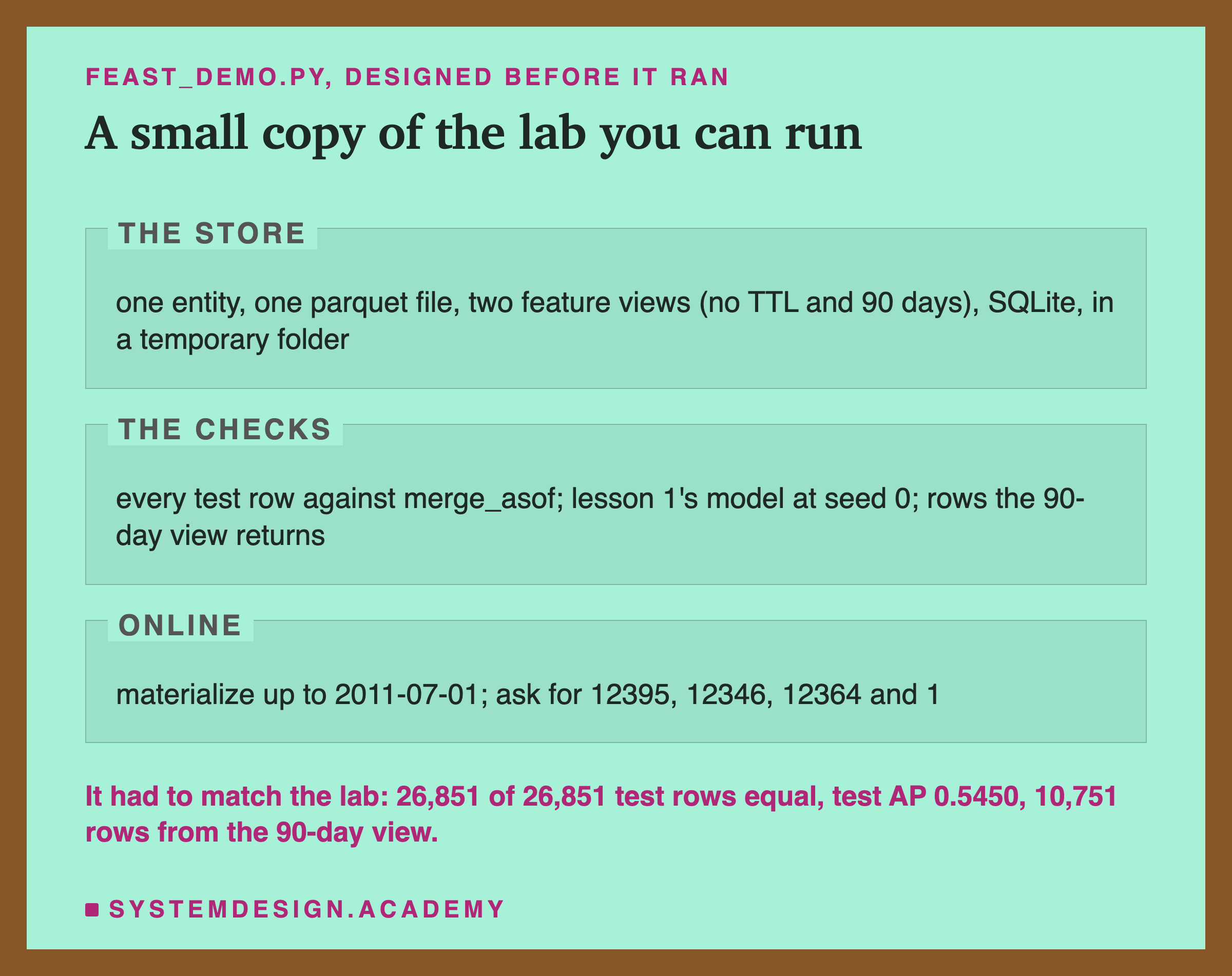
I wrote the demo's design into its docstring after the lab had run and before the demo first ran. It builds its snapshot table with its own short code, so it is also a second check of the lab.

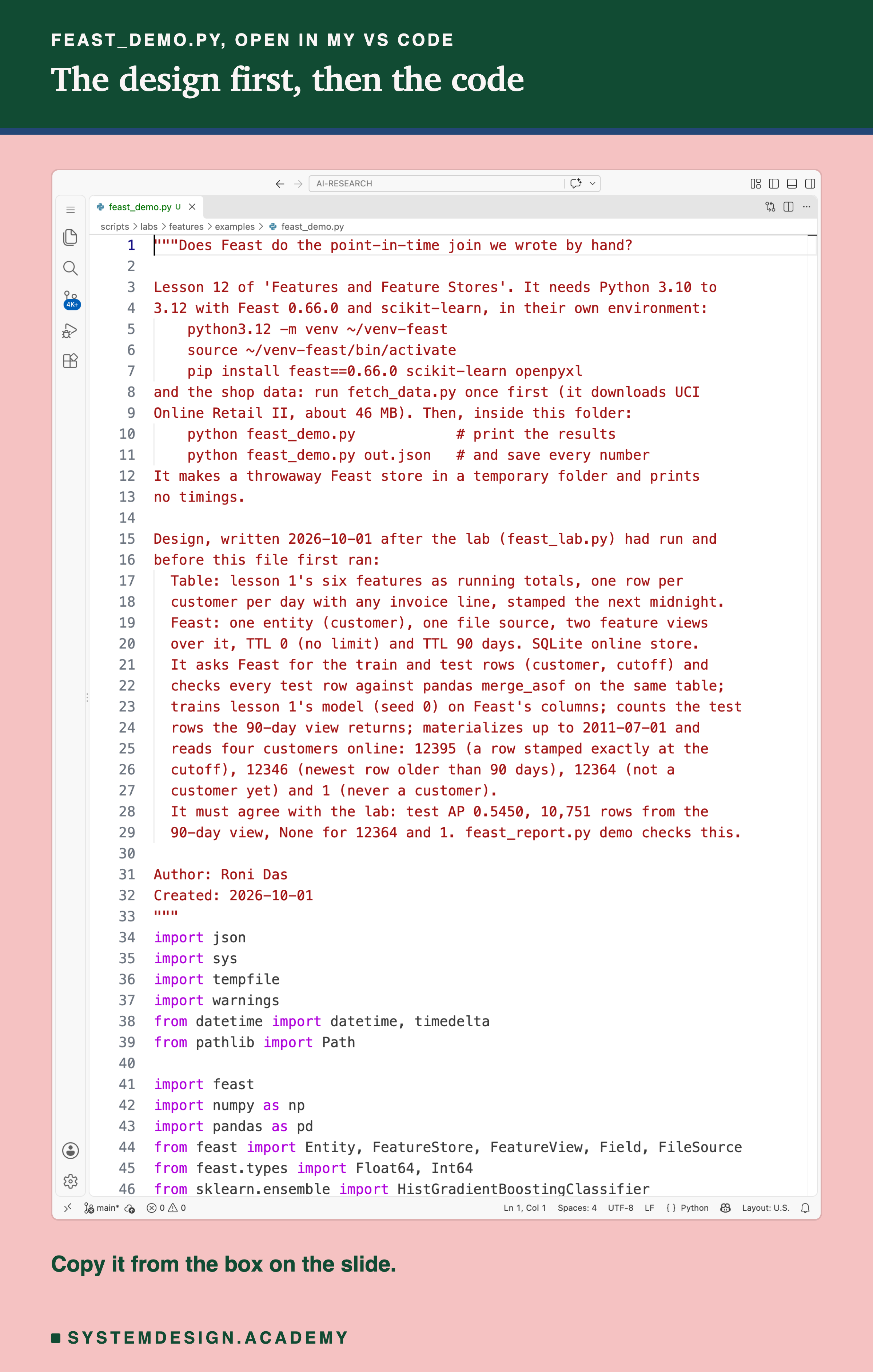
Before you run this lab. Feast needs its own environment. Feast's tested range is Python 3.10 to 3.12. On a Mac or Linux, make one and turn it on with python3.12 -m venv ~/venv-feast and then source ~/venv-feast/bin/activate. On Windows, the activate script is in the environment's Scripts folder instead. Then install the pinned versions: pip install feast==0.66.0 scikit-learn==1.9.1 openpyxl. openpyxl is only needed by fetch_data.py, to read the shop's Excel file. First run python fetch_data.py from the scripts/labs/features folder. It downloads the shop data once, about 46 MB, and writes one cleaned file.

The demo imports task.py from that same folder. It needs no GPU and no server. I ran it only on a Mac, with Python 3.12, so I have not checked it on Windows or Linux. Give it a file name, , and it also saves every number. That is how was made.

This box holds two real customers' snapshot tables, exactly as Feast stored them. Customer 12395 has a row stamped exactly at the cutoff. Customer 12346's newest row before July 2011 is from January. It does Feast's join rule in plain Python, so it runs in your browser with nothing installed.

Press Run. It shows which row the join picks at the cutoff, and what Feast itself returned. Then try three things. Set TTL_DAYS = 90 and CUSTOMER = 12346: the row disappears, as it did in Feast. Set INCLUSIVE = False: customer 12395 falls back to an older row. Change CUTOFF to another date and watch the chosen row move.

The report script writes this box from the lab's stored results. Then it runs the box for both customers, with and without the TTL, and checks that each answer equals what Feast returned. The rule in the box is short, which is the point: a point-in-time join with a TTL is only two comparisons and "newest wins".

The lab is one file, scripts/labs/features/feast_lab.py, and it runs in the Feast environment. It imports lesson 1's and lesson 2's lab files instead of copying them, so the comparisons are against their real code.

daily_snapshot builds lesson 1's six features as running values. It sorts the lines by customer, keeping time order, and uses pandas' running sums and counts. Two counts need care: an invoice or a product counts only the first time it appears. Then it keeps the last line of each customer's day and stamps it at the next midnight. l2_table calls lesson 2's own feature_table and adds whole-second versions of its times.

feast_hist hands the entity rows to get_historical_features, with a row number, so the answer can be matched back. It records how many rows went in and how many came back. That count is how the missing rows were found. asof is the same join done with merge_asof, for the comparison, and compare counts exactly equal values, column by column.

main applies the three feature views, runs the three historical reads and the comparisons, trains the model, and then runs materialize and the online reads. latency is the timing step, which checks the load average first and skipped itself. The report, , has its own code for every check, as the report slide describes.

These are the steps I would follow to build training rows with Feast, or with any feature store.

1. Stamp each row with the moment it became true. For a nightly job, that is the midnight after the day it covers. Then an inclusive join is correct. Write down what your stamps mean.

2. Make the entity table yourself, with a row number. One row per customer and cutoff, with the cutoff in a column called event_timestamp. Feast sorts the rows by time inside the join, so keep a row number to match them back. Do not send the same customer and time twice: the file store keeps one answer per pair.

3. Count the rows that come back. If fewer come back than you sent, find out why before you train. Here a TTL removed 41,232 rows with no error. Even with no TTL, a row dated before a customer's first snapshot disappears from the file store's output, so new customers need their own handling.

4. Choose the TTL on purpose. A TTL of zero means no limit. Use a real TTL only for values that go stale. For running totals over a customer's whole history, a TTL deletes true information.

5. Compare the store's answer with a join you wrote yourself, once. A small merge_asof on a sample is enough. Here the two matched on every row, and now I trust it.

6. Read the same customer online and offline. After materializing, check that the online answer equals the historical answer at the same moment, and decide what your service does with None.

Use a feature store like Feast when several models or services read the same features. It also helps when the team that builds features is not the team that trains models. Then one description for both training and serving is worth a lot, as lesson 5 showed when two programs disagreed. It also helps when people keep writing the point-in-time join by hand and getting it wrong, as lesson 2 showed can happen.

A hand-written join is fine for a one-person project where one script builds the features and trains the model together. Here, Feast and merge_asof gave the same rows. The join itself was not the hard part. Getting the stamps right, which lesson 2 did, was the hard part, and Feast does not do that for you.

Do not expect a feature store to compute your features. In this lab, I built every running total myself and gave Feast a finished table. Feast joined and served it. Feast can also run Python code at read time, in on-demand feature views, which lesson 5 described, but I did not use them here.

Be careful with any setting that has a different effect online and offline. The TTL in this lab is the example: it removed customers from training, and did nothing at serving.

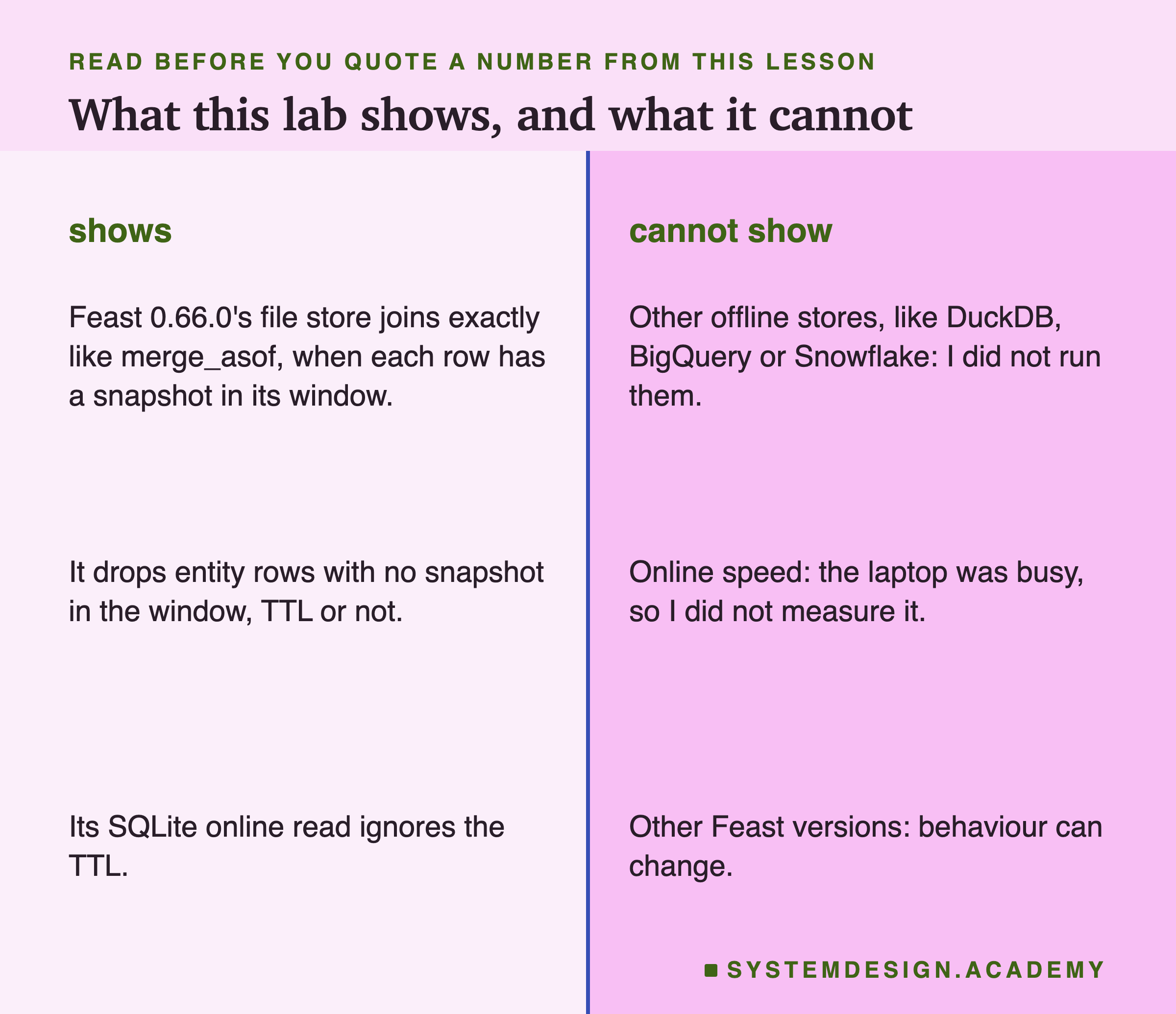
One version and one pair of stores. Everything here is Feast 0.66.0, with the file offline store and the SQLite online store. Other offline stores use different code, and a different version could behave differently. The dropped rows, with or without a TTL, and the ignored TTL online are facts about this setup only.

One shop and one kind of feature. My features were running totals, stamped once a day. A store with many updates per second, or features that really do go stale, would test other parts of Feast. I did not test them.

No speed numbers. The laptop was busy, so I measured no timing, and quote none.

Guesses informed by the code. I read the source before the run, so my right guesses confirm the code, not something beyond it. Two parts were added after the results, and both are labelled: the reason money matched, and the chart of row ages. Two more checks were added after an independent review: rows from before a first snapshot with Feast's docs example, and which pandas sums compensate.

This is the last lesson of the chapter, so here is all of it on one page. Every number in the two figures was read from that lesson's own results file by the figure script, and I copied them into the text below.

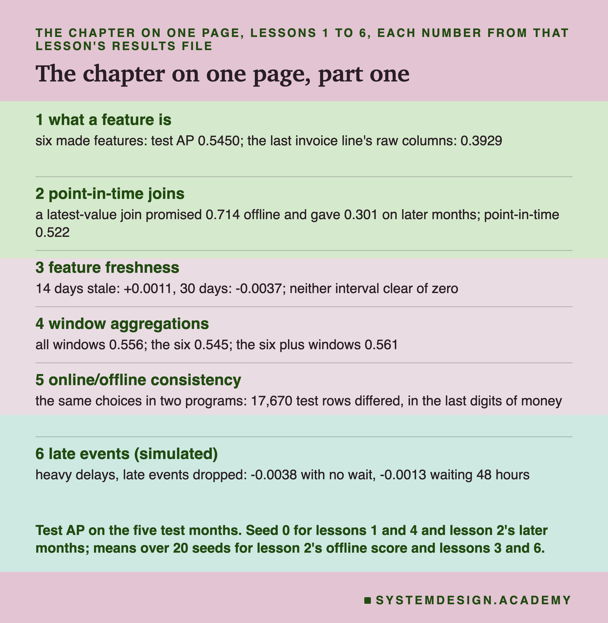
Lesson 1 asked whether a better model or a better feature is worth more. Six simple features made from each customer's history scored a test AP of 0.5450, against 0.3929 for the raw columns of their last invoice line. Tuning the model on the raw columns added almost nothing. Lesson 2 showed that joining each customer's latest values promised 0.714 offline and gave 0.301 on later months, while the correct point-in-time join gave 0.522.

Lesson 3 served features up to 30 days stale. At 14 days the change was +0.0011 and at 30 days -0.0037, and neither could be told apart from luck. Lesson 4 tried windows of days: all of them together scored 0.556, the six features 0.545, and both together 0.561. Lesson 5 wrote each feature twice, in batch and event by event, and found 17,670 test rows that still differed, only in the last digits of money. Lesson 6 simulated late events. When heavy delays meant late events were dropped, AP fell by 0.0038 with no wait, and by 0.0013 when the pipeline waited 48 hours.

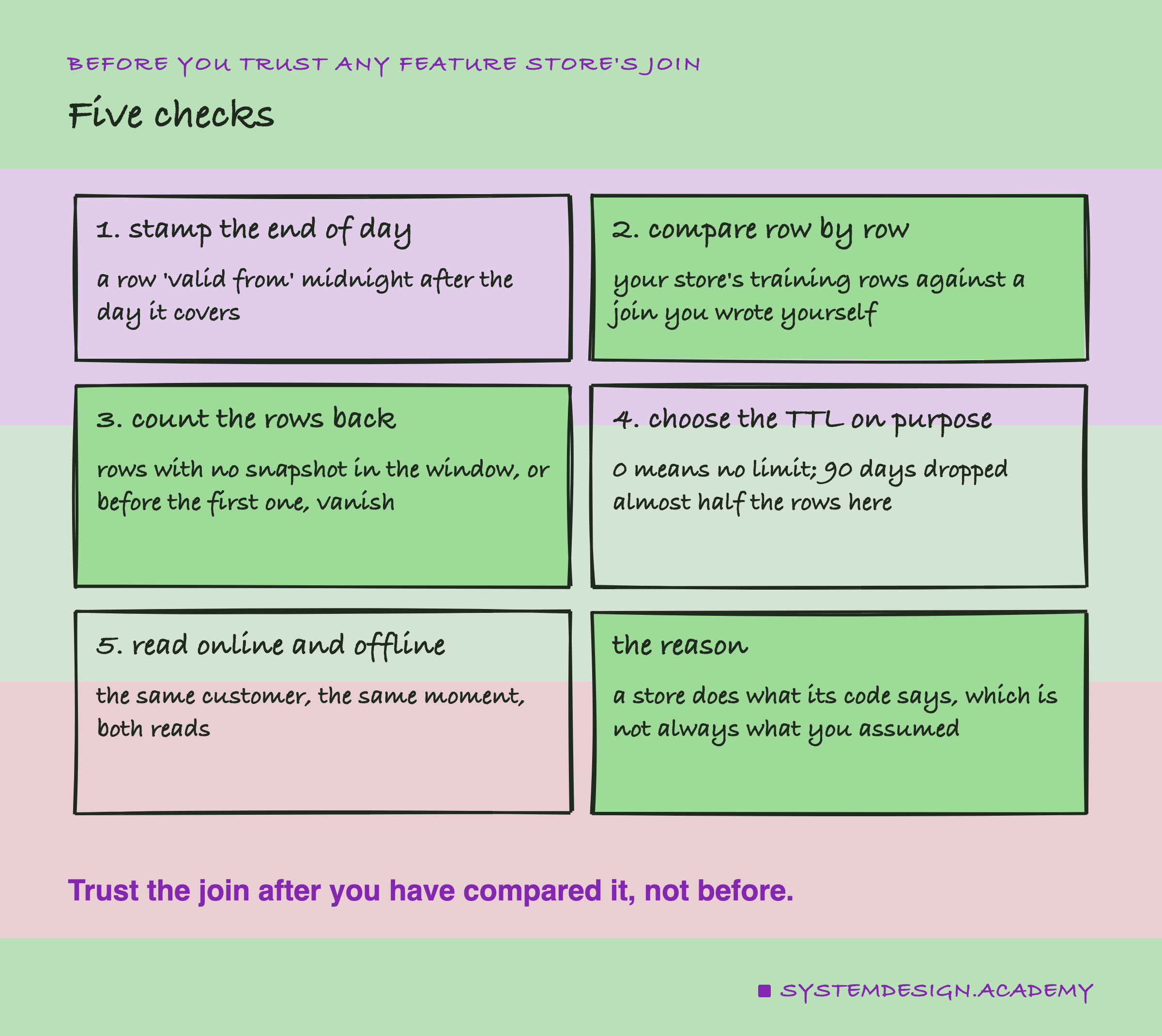
If you already use a feature store, here is one thing to do on Monday. Take one training set it built, and count its rows. Compare the count with the number of entity rows you sent. If they differ, find out which rows went missing and why, before your next training run.

If you are about to adopt one, write a small merge_asof join for one month of data and compare it with the store's historical read, row by row. In this lab it took a few lines, and it turned "I hope the store is right" into "I checked, on every row".

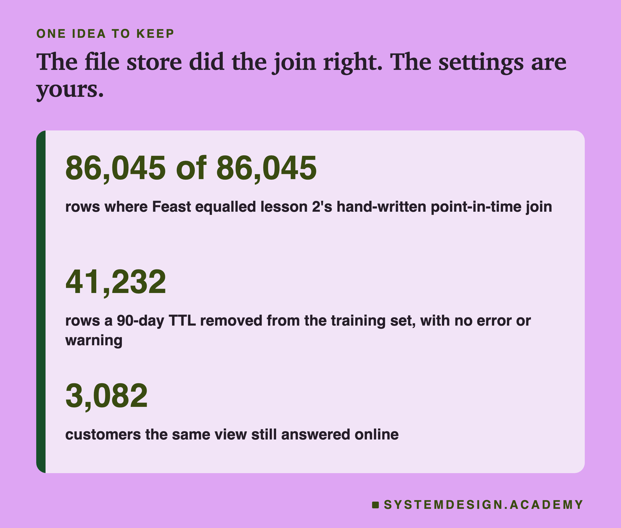
The one idea to keep: a good feature store does the point-in-time join correctly. Feast's file store did it on every row that had a snapshot in its window. What it cannot do is choose your settings. A stamp, a TTL or a missing customer can still change your training data quietly. Compare once, count the rows, and read both sides.